1. Introduction
With the rapid development of technology and the increasing trend of population aging, robots are playing an increasingly important role in social life. In the manufacturing industry, robots have become a core component of automated production lines. Collaborative robots and new logistics robots are driving the development of flexible manufacturing [Reference Waseem and Chang1] and intelligent warehousing. They can perform high-precision and high-efficiency tasks, significantly improving production efficiency and product quality. In the healthcare field, robot technology is also changing the form and quality of medical services. Surgical robots [Reference Boal, Di Girasole, Tesfai, Morrison, Higgs, Ahmad, Arezzo and Francis2] can assist doctors in performing precise, minimally invasive surgeries, improving surgical success rates. Rehabilitation robots help patients with rehabilitation training, accelerating the recovery process. In the agricultural sector, agricultural robots [Reference Guo, Wang, Mao, Wang, Wu, Wu and Liu3] are promoting the development of smart agriculture. They can precisely perform tasks such as planting, fertilizing, and spraying pesticides, improving agricultural production efficiency. As technological innovation continues and the scope of applications expands, robots with improved self-learning and operational capabilities are becoming increasingly prevalent and influential across diverse areas. These advancements not only hold substantial theoretical value but also present profound societal significance and practical application prospects.
Robot learning [Reference Kumar, Ray and Ansari4] enables robots to acquire the ability to autonomously learn and execute tasks. Robot learning refers to the process where robots continuously improve their skills and strategies through self-exploration and learning. The core of this method lies in utilizing artificial intelligence technologies such as machine learning to allow robots to automatically adjust and optimize their behavior through interactions with the environment, thus achieving self-learning [Reference Kroemer, Niekum and Konidaris5]. Robot learning requires robots to have the ability to perceive the surrounding environment in real time [Reference Liang, Munson and Kientz6] and interact with it [Reference Liang, Munson and Kientz6]. With traditional robot control methods, robots cannot pre-acquire environmental parameters and task models for complex and variable environments, resulting in ineffective interactions with the surrounding environment and an inability to complete tasks. Reinforcement learning (RL) is considered as the well-performing machine learning algorithm, which guarantees to obtain actions by the agents in an environment to maximize the rewards [Reference Gawali and Gawali7]. RL enables robotic agents to continually improve their decision-making and control strategies through direct interaction with the environment, receiving environmental feedback in the form of rewards and penalties. This trial-and-error mechanism allows for the discovery of optimal or near-optimal solutions in complex, uncertain, and dynamic scenarios without explicit supervision. With advances in deep learning techniques, deep reinforcement learning (DRL) further enhances the scalability and representational power of RL, making it applicable to high-dimensional sensory inputs and intricate manipulation tasks.
Using RL for robot control [Reference Zhu and Zhang8] does not require pre-established control strategies but instead allows robots to autonomously learn methods and strategies to solve tasks through interactions with the environment. In this process, the robot’s policy network is continuously iterated and updated until the policy network converges and the robot learns an optimal task-solving strategy. With the continuous development of artificial intelligence technologies, robot learning methods will continue to be improved and perfected, providing broader prospects for the development and application of robots.
Building upon these advancements, this study develops a robotic arm learning system that synergistically combines DRL with imitation learning under the multi-sensor information fusion paradigm to achieve autonomous and robust door-opening maneuvers.
The main contributions of this work are as follows: (1) we improve the soft actor-critic (SAC) algorithm by incorporating Wasserstein generative adversarial network (WGAN)’s gradient penalty, resulting in SAC-gradient penalty (SAC-GP), which enhances learning stability and efficiency. By further integrating generative adversarial imitation learning (GAIL)-based imitation learning, the algorithm achieves higher performance and faster convergence. Experiments – including block lifting and door-opening tasks – demonstrate superior performance and efficiency compared to baseline methods. (2) We construct both simulation and real-world experiment environments. The simulation is built on the MuJoCo physics engine with the robosuite framework. The real-world setup employs a Sawyer robot with an AG-95 gripper as actuators, combined with a NOKOV optical motion capture system and a six-axis Srisensor force sensor for perception. (3) We deploy agents trained in simulation to the real Sawyer platform for tasks such as grasping, rotating, pulling, and opening a door handle. Experimental results show that the proposed self-learning system exhibits high functional completeness in both hardware and algorithm, strong learning and execution capabilities for complex tasks, and exhibits stable and smooth operation in real-world conditions.
2. Related work
RL is a method that solves decision optimization problems through interactive learning [Reference Xu, Zhao, Lu and Zhang9]. Its core idea is that an agent attempts different actions and observes the results through interactions with the environment, learning how to maximize the cumulative reward from the environment and ultimately finding the optimal strategy to achieve the goal. Due to their excellent ability to approximate nonlinear functions and extract relevant features from raw inputs, deep neural networks have been introduced into RL, leading to the emergence of DRL [Reference Cao, Ni, Kawaguchi and Hashimoto10]. As a bridge connecting deep learning and RL, DRL combines the perceptual capabilities of deep learning with the decision-making capabilities of RL, enabling the autonomous decision-making of the agent through end-to-end learning [Reference Lyu, Shen and Zhang11].
Tuomas [Reference Haarnoja, Zhou, Abbeel and Levine12, Reference Haarnoja, Zhou, Hartikainen, Tucker, Ha, Tan, Kumar, Zhu, Gupta, Abbeel and Levine13] proposed the SAC algorithm, which is based on the maximum entropy RL framework and aims to improve exploration, stability, and sample efficiency by maximizing the expected return and entropy of the policy. This method encourages the agent to perform actions as randomly as possible when executing tasks, enhancing exploration and robustness. To demonstrate the effectiveness of the SAC algorithm, the authors validated it on a three-finger, dexterous robotic hand platform. After 20 h of training, the robotic hand learned the strategy of rotating valves through image input and successfully completed the task.
Guo [Reference Guo, Ren, Lai, Wu and Xie14] proposed a RL algorithm based on SAC, which achieves real-time optimal feedback control by using a composite auxiliary reward structure and sum-tree priority experience replay (SAC-SP). This method can achieve real-time navigation of automated guided vehicles (AGVs) in various obstacle scenarios and high-accuracy prediction of optimal trajectories under unknown conditions.
Cao [Reference Cao, Ni, Kawaguchi and Hashimoto10] proposed combining path planning (PP) control and the SAC algorithm, where PP control is responsible for steering while the SAC algorithm handles speed control, establishing a complementary relationship between the two. This combination allows PP control to compensate for the deficiencies of the SAC algorithm through adaptive speed adjustment, thereby improving path convergence. Their simulation and experimental results demonstrate that the algorithm is easy to train and has advantages in tracking paths with different curvatures.
In specific applications, DRL often requires more training time and computational resources and may be affected by sparse rewards and difficulties in exploration in some cases, greatly increasing training costs and reducing training efficiency [Reference Li, Zhang and Guo15]. Demonstration learning is a paradigm in which an agent learns to perform a task by imitating the behavior of an expert shown in demonstrations [Reference Liu, Wen, Guo and Liu16]. Therefore, people have considered combining demonstration learning and RL to address the issue of low sample utilization efficiency and improve training efficiency [Reference Liu, Zeng, Ma, Pan, Gao and Zhang17].
Huang [Reference Huang, Chen, Li, Liu and Dou18] proposed an efficient RL algorithm named demonstration-guided exploration (DEX), which combines RL with demonstration learning to overcome exploration issues in surgical robots. This method effectively utilizes expert data to improve exploration efficiency. It uses nonparametric regression to estimate higher values for behaviors similar to those of experts, promoting productive interactions. Extensive experiments on 10 surgical manipulation tasks on the surgical simulation platform SurRoL showed that the designed method significantly improves exploration efficiency and task success rates.
Zhu [Reference Zhu, Wang, Merel, Rusu, Erez, Cabi, Tunyasuvunakool, Kramár, Hadsell, de Freitas and Heess19] proposed a method combining RL and demonstration learning, using teaching data to reduce the difficulty of exploration in continuous domains and utilizing this data to accelerate and stabilize the learning of visual–motor policies in multi-stage tasks. This method enables end-to-end learning, learning directly from pixel inputs and making actions through a visual–motor controller. The authors evaluated their method on six different manipulation tasks, including stacking blocks and pouring water, and validated it on real robots.
Wu [Reference Wu, Escontrela, Hafner, Goldberg and Abbeel20] proposed the DayDreamer algorithm, which addresses the learning problem for robots executing tasks in complex environments. This algorithm combines actor-critic networks from RL and reduces the number of trial-and-error attempts in the real environment by planning within the learned world model. The authors applied the DayDreamer algorithm to four different robots, demonstrating its ability to learn in the real world. These robots included a quadruped robot, two different robotic arms, and a wheeled robot. The tasks covered various challenges, including continuous and discrete actions, dense and sparse rewards, proprioception and camera inputs, and sensor fusion with multiple input modes.
Furthermore,recent advances have paid considerable attention to skill transfer and generalization in human–robot interaction. For example, Gawali and Gawali [Reference Gawali and Gawali7, Reference Gawali and Gawali21] proposed a “Transfer Expert Reinforcement Learning (TERL)” framework, which enables skill knowledge transfer between humans and robots. Their approach integrates modified RL with an improved Coyote Optimization Algorithm (BWF-COA) to tune the action features of robotic arms. By employing a deep neural network to process input kinematic movements, their method facilitates the effective transfer of movement strategies. Experimental results demonstrate that such optimized skill transfer models can significantly reduce prediction errors and enhance policy rewards compared to traditional approaches, highlighting the importance of optimization-driven learning in autonomous robot control.
3. Preliminaries
3.1. Soft actor-critic
SAC [Reference Haarnoja, Zhou, Abbeel and Levine12, Reference Haarnoja, Zhou, Hartikainen, Tucker, Ha, Tan, Kumar, Zhu, Gupta, Abbeel and Levine13] is a modern off-policy DRL algorithm that combines policy-based and value-based methods for efficient policy learning and optimization in continuous action spaces. Its core idea is to maximize expected returns while maintaining the randomness of the policy, which helps the agent improve the efficiency of exploring the environment and find better policies. “Soft” in the algorithm refers to the introduction of the concept of entropy during training the policy, making the policy have a certain degree of randomness. This randomness helps the algorithm achieve a balance between exploration and exploitation of existing policies, enabling it to discover and utilize better policies. In addition, the SAC algorithm also employs entropy optimization methods, where the entropy term of the policy is added to the objective function to encourage exploratory behavior, effectively preventing the policy from prematurely falling into local optima.
The maximum entropy objective extends the standard objective by simultaneously maximizing the target and the entropy, as shown in Eq. (1). The SAC algorithm encourages policy exploration through maximum entropy, enabling the model to learn more near-optimal policies and ensuring the robustness of the model:
 \begin{equation} \pi ^{*}=\arg \max _{\pi } \sum _{t} \mathbb{E}_{\left (s_{v}, a_{i}\right ) \rho _{\pi }}\left [r\left (s_{t}, a_{t}\right )+\alpha \mathcal{H}\left (\pi \left (\cdot \mid s_{t}\right )\right )\right ] \end{equation}
Among them,
 $\pi ^{*}$
denotes the optimal policy,
 $\pi$
is a candidate policy,
 $t$
is the time step,
 $s_{t}$
is the state at time
 $t$
,
 $a_{t}$
is the action at time
 $t$
,
 $\rho _{\pi }$
represents the trajectory distribution under policy
 $\pi$
,
 $r\left (s_{t}, a_{t}\right )$
is the reward function,
 $ \mathcal{H}(\pi (\cdot \mid s))=-\mathbb{E}_{a} \log \pi (a \mid s)$
represents the entropy term, and
 $ \alpha$
is the temperature coefficient, which determines the importance of the entropy term in the return function; thus, it controls the degree of randomness in the optimal policy.
In the SAC algorithm,
 $ \alpha$
is an important hyperparameter, which controls the degree of randomness of the strategy. The higher the
 $ \alpha$
, the more inclined the strategy is to choose random actions; The lower the
 $ \alpha$
, the more inclined the strategy is to choose deterministic actions. The SAC algorithm adaptively adjusts the parameters to achieve a balance between exploration and utilization.
Compared to other algorithms, SAC’s advantage lies in its ability to maximize expected returns while maintaining policy randomness, which improves the algorithm’s exploration efficiency in complex environments. SAC further enhances its performance and stability through techniques such as entropy optimization and adaptive temperature parameters.
3.2. Generative adversarial imitation learning
Demonstration learning is a process of learning and improving decision-making abilities by observing the behavior of demonstrators. Learning from expert demonstrations allows for a more natural and easier generalization of the expert’s strategy to the current observed situation [Reference Levine, Popović and Koltun22]. GAIL is a method of demonstration learning. Its goal is to enable agents to acquire the ability to perform tasks through expert demonstrations. The core idea of GAIL is to compare and learn the robot’s own behavior and policy with the behavior and policy demonstrated by experts through a generative adversarial network (GAN), thus achieving demonstration learning.
In GAIL, the generator acts as the policy network, responsible for generating the agent’s behavior, while the discriminator plays the role of a binary classifier, dedicated to distinguishing whether the input behavior data originates from demonstration data or forged data produced by the generator. The generator aims to create forged data, while the discriminator strives to accurately distinguish between demonstration data and behavior data generated by the generator. Through this adversarial training process, the generator ultimately learns and generates strategies that are highly similar to the demonstration behavior.
In GAIL, the input to the generator is the state of the environment that the agent is currently in, and the output is the action that the agent should perform in the current state. The input to the discriminator is a state–action pair, that is, the behavior of an agent in a particular state. The output of the discriminator is a probability value that represents the likelihood of the input’s state–action pair coming from the expert data. For real expert data, this probability value should be accepted close to 1, and for data generated by the generator, this probability value should be close to 0.
Ishaan [Reference Gulrajani, Ahmed, Arjovsky, Dumoulin and Courville23] proposed gradient penalty for WGANs. GANs use
 $D\left ( .;\,\omega \right )$
to represent the discriminator and use
 $G\left ( .;\,\theta \right )$
to represent the generator, learning through the use of the discriminator’s loss function’s stochastic gradient
 $\tilde {g}\left ( \theta ,\omega \right )$
and the generator’s loss function’s stochastic gradient
 $\tilde {h}\left ( \theta ,\omega \right )$
. When the true gradients are denoted as
 $g\left ( \theta ,\omega \right ) =\nabla _{\omega }\mathcal{L}_D$
and
 $h\left ( \theta ,\omega \right ) =\nabla _{\theta }\mathcal{L}_G$
, these stochastic gradients can be defined as:
 \begin{equation} \left \{ \begin{array}{l} \tilde {g}\left ( \theta ,\omega \right ) =\nabla _{\omega }\mathcal{L}_D+M^{\left ( \omega \right )}\\[5pt] \tilde {h}\left ( \theta ,\omega \right ) =\nabla _{\theta }\mathcal{L}_G+M^{\left ( \theta \right )}\\ \end{array} \right . \end{equation}
In this formula,
 $\mathcal{L}_D$
is the loss function of the discriminator,
 $\mathcal{L}_G$
is the loss function of the generator, and
 $M^{\left ( \omega \right )}$
and
 $M^{\left ( \theta \right )}$
are random variables representing the noise introduced by stochastic gradient estimation, while
 $\tilde {g}\left ( \theta ,\omega \right )$
and
 $\tilde {h}\left ( \theta ,\omega \right )$
are stochastic approximations of the true gradients.
The goal of gradient penalty is to introduce a gradient penalty term to improve the training process of WGANs, thereby avoiding issues caused by weight clipping and enhancing the performance of the GAN. This method introduces a gradient penalty term into the loss function, making the gradient norm of the discriminator closer to 1, thus satisfying the 1-Lipschitz constraint, which enhances the stability of training and the quality of the generated samples. Specifically, the form of the gradient penalty is given as:
 \begin{equation} L_{\text{gp}}=\lambda \mathbb{E}\hat {x}\sim P\hat {x}\Big [ \big ( ||\nabla _{\hat {x}}\, f ( \hat {x} ) ||_2-1 \big ) ^2 \Big ] \end{equation}
where
 $L_{gp}$
is the gradient penalty term added to the discriminator’s loss function,
 $\lambda$
is a hyperparameter controlling the strength of the gradient penalty,
 $P\hat {x}$
represents the linear interpolation distribution between real data and generated data,
 $f\left ( \hat {x} \right )$
is the discriminator’s score for sample
 $\hat {x}$
, and
 $\nabla _{\hat {x}}\, f\left ( \hat {x} \right )$
is the gradient of the discriminator with respect to sample
 $\hat {x}$
.
4. Method
4.1. Algorithm improvements
In this work, we formulate the control policy for robotic manipulation as a Markov decision process (MDP) [Reference Li, Zhang and Guo15], where the agent observes the system state and selects actions according to a parameterized policy. The RL algorithm is employed to optimize the policy by maximizing the expected cumulative reward. This data-driven policy serves as the control law for the robot, mapping observations to actions in a closed-loop manner, functionally equivalent to a classical feedback controller [Reference Sutton and Barto24, Reference Recht25]. As in conventional control design, we view the RL-trained policy as a closed-loop feedback controller. Our policy maps the robot’s state to control actions at every timestep, following the structure and operational logic of a feedback control system.
Similar to WGANs, this paper introduces a gradient penalty term into the SAC loss function. This term calculates the gradient norm of the policy network (actor) in the state space and penalizes it accordingly. By doing so, the policy network tends to maintain a certain degree of continuity during parameter updates, avoiding overly drastic changes. Meanwhile, SAC must maintain a balance between exploration and exploitation during the policy optimization process. The gradient penalty term in WGAN-GP has been shown to help maintain diversity in the generated samples by encouraging smooth and continuous changes in the output [Reference Gulrajani, Ahmed, Arjovsky, Dumoulin and Courville23]. Inspired by this, introducing a gradient penalty into the SAC framework can likewise encourage diversity in the action space and improve training stability. Therefore, introducing the concept of the gradient penalty into SAC can encourage the policy network to generate actions that maintain diversity in the action space, preventing premature convergence to local optimal solutions.
In this study, the gradient penalty is applied to the loss calculation for the policy network. The update rule for the policy network (actor) is given as:
 \begin{equation} \theta _{n+1}=\theta _n+a\left ( n \right ) \left ( s_n,a_n,\theta _n \right ) d\left ( s_n,s_{n+1},\omega _n \right ) \end{equation}
In this formula,
 $\theta _{n}$
is the parameter vector of the actor network at iteration
 $n$
,
 $ a\left ( n \right )$
is the learning rate at iteration
 $n$
,
 $d\left ( s_n,s_{n+1},\omega _n \right )$
is the temporal-difference (TD) error or advantage function, capturing the update direction,
 $e_n$
is an eligibility trace or scaling factor associated with the sample at iteration,
 $s_n$
is the observed state at iteration
 $n$
,
 $a_n$
is the chosen action at iteration
 $n$
, and the likelihood ratio derivative
 $\Psi \in \mathbb{R}^m\theta$
is defined as:
 \begin{equation} \Psi (s, a, \theta )=\frac {\nabla _{\theta } \pi (a\mid s)}{\pi (a\mid s)} \end{equation}
In this formula,
 $\pi (a\mid s)$
is the policy’s probability of selecting action
 $a$
in state
 $s$
, parameterized by
 $\theta$
, and
 $\nabla _{\theta } \pi (a\mid s)$
is the gradient of the policy with respect to its parameters
 $\theta$
.
In the SAC algorithm, the original loss function for the policy network typically consists of a policy gradient loss term and an entropy regularization term. Now, a gradient penalty term is added to obtain the new loss function. Assuming the policy network
 $ \pi$
has parameters denoted by
 $ \theta$
, the gradient of the policy network’s output actions with respect to the state can be calculated as:
 \begin{equation} \nabla _{a} \log \pi (a\mid s;\,\theta ) \end{equation}
where
 $\pi (a\mid s;\,\theta )$
is the policy network (actor), which outputs the probability of taking action
 $a$
given state
 $s$
, parameterized by
 $ \theta$
.
Then, the
 $L2$
norm of this gradient is calculated, and a target norm r is defined. The gradient penalty term can be expressed as:
 \begin{equation} \lambda \mathbb{E}_{s \sim p, a \sim \pi } \left [\left (\lvert \nabla {a} \log \pi (a \mid s ;\, \theta )\lvert _{2}-r\right )^{2}\right ] \end{equation}
In this equation,
 $ \lambda$
is the gradient penalty coefficient, a hyperparameter that controls the strength of the penalty term;
 ${E}_{s \sim p, a \sim \pi }$
is expectation over states
 $s$
sampled from the state distribution
 $p$
and actions
 $a$
sampled from the policy
 $\pi;$
and
 $\nabla {a} \log \pi (a \mid s ;\, \theta )$
is the gradient of the log-probability of action
 $a$
with respect to
 $a$
, given state
 $s$
and parameters
 $\theta$
.
Finally, by adding the gradient penalty term to the original loss function of the actor network, we obtain the new loss function:
 \begin{equation} L_{\text{actor}}^{\text{with }\mathrm{GP}}=L_{\text{actor }}+\lambda \mathbb{E}_{s\sim \rho, a\sim \pi }\left [\left (\lvert \nabla _{a} \log \pi (a\mid s;\,\theta )\lvert _{2}-r\right )^{2}\right ] \end{equation}
This new loss function combines the policy gradient loss term, entropy regularization term, and gradient penalty term from the SAC algorithm. By introducing the gradient penalty term, the following advantages are achieved:
-
1. Improved policy stability: Gradient penalty encourages the actions generated by the policy network to maintain diversity in the action space, preventing the policy from falling into local optima. This allows the agent to better adapt to environmental changes and improve task success rates.
-
2. Enhanced exploration capabilities: The SAC algorithm inherently encourages exploration, and the addition of the gradient penalty term further enhances this ability. Through the gradient penalty term, the algorithm can better balance exploration and exploitation strategies, thereby finding the optimal policy more quickly.
-
3. Increased training efficiency: The inclusion of the gradient penalty term helps reduce instability and fluctuations during the training process, further improving training efficiency.
-
4. Improved task completion quality: By optimizing the loss function, errors during task completion can be reduced, thereby enhancing the efficiency and quality of task completion.
This study integrates the GAIL algorithm into the SAC-GP algorithm. In GAIL, the generator attempts to optimize its policy to deceive the discriminator, whereas in SAC-GP, the policy network optimizes by maximizing the expected return and entropy. This research combines the adversarial loss from GAIL with the policy optimization loss from SAC-GP, which consists of maximizing the expected return and entropy regularization, to form a hybrid loss function. This loss function balances the two objectives, enabling the robotic arm learning system to perform imitation learning while maintaining sufficient exploration.
4.2. Construction of a self-learning system for robotic arms
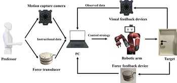
The robotic arm learning system and its components built in this study are shown in Figure 1.
The composition of a robotic arm self-learning system.

The real-world experimental platform is built on the robot operating system (ROS), which integrates the control of the Sawyer robotic arm, the AG-95 gripper, and data acquisition from a NOKOV optical motion capture system and a six-axis Srisensor force/torque sensor. All algorithms are implemented in Python 3 with the PyTorch library. To thoroughly validate the effectiveness of the proposed GAIL + SAC-GP algorithm, both a virtual simulation environment and a real-world physical platform are constructed. The simulation environment is developed using the MuJoCo physics engine [Reference Todorov, Erez and Tassa26] and the RoboSuite framework [Reference Zhu, Wong, Mandlekar, Martín-Martín, Joshi, Nasiriany and Zhu27]. MuJoCo is widely used for simulating complex robot–environment interactions, while RoboSuite provides various robot tasks and user-friendly interfaces for robot learning research. In our workflow, the agent is first trained in the virtual environment, where it optimizes its policy through iterative trial-and-error learning. Once the policy converges, we apply Sim2Real (Simulation to Reality) transfer [Reference Zhu, Lin, Jain and Zhou28–Reference Sandha, Garcia, Balaji, Anwar and Srivastava32] to directly deploy the trained agent on the real hardware without further real-world training, thereby enabling immediate evaluation and rapid deployment. Ensuring high consistency between simulation and reality is critical in this process. The following sections further elaborate on the construction of both environments and the corresponding training/evaluation processes.
4.3. Environment setup
The construction of the virtual environment is based on the RoboSuite robot simulation framework. The setup task scenario is illustrated in Figure 2.
Construction of a virtual environment for door handle task.

The hardware platform of the robotic arm learning system mainly involves a computing platform, a robotic arm, an electric gripper, visual feedback equipment, and force feedback equipment. To realize task scenarios in a real environment, this study has built a learning system platform for the robotic arm, as shown in Figure 3.
The basic composition of the learning system platform for a robot.

In the hardware composition of this robotic system, the visual feedback equipment uses the NOKOV optical motion capture system, the force feedback equipment employs the SRI six-axis force sensor, the computing platform is a desktop PC, the robotic arm adopts the Sawyer collaborative robot from Rethink Robotics, and the gripper uses the DAHUAN AG-95 series gripper. Among them, the computing platform’s CPU is an AMD 2970WX with 24 cores and 48 threads and a base frequency of 3.0 GHz. The computer’s memory is 128 GB, and the graphics card model is the NVIDIA RTX 3,090.
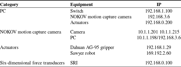
The IP address of the hardware device.

Control system hardware composition.

This article chooses to build the software platform under the Ubuntu 18.04 operating system, using ROS Melodic to construct the control system and implement data communication functions. The hardware composition of this control system is illustrated in Figure 4. The IP addresses of each device are detailed in Table I.
This study first trains agents in a virtual simulation environment and then deploys the trained agents to the real environment through Sim2Real. In Sim2Real, it is necessary to ensure a high degree of consistency between the simulation environment and the real environment. Therefore, the real environment interface is strictly written according to the interface format in RoboSuite, making the interfaces of the virtual simulation environment and the real environment consistent. In addition, this paper also unifies the spatial coordinate system and spatial units in the virtual and real environments. Ultimately, the environmental state information dimension and action space dimension in the real environment are kept consistent with those in the simulation environment to satisfy the requirements of Sim2Real.
4.4. Multi-source sensor information fusion
The mechanical arm learning method studied in this paper utilizes two types of sensors: NOKOV motion capture cameras and SRI six-dimensional force sensors. To fully leverage the advantages of these two sensors, it is necessary to effectively fuse the information provided by them, thus providing more comprehensive and accurate information. Each sensor has its own unique measurement capabilities and limitations, and through fusion, errors or biases that may exist in a single sensor can be eliminated, improving the reliability of the overall data. Based on the importance of the two modal information, this paper actively adjusts their advantages in the fused features and performs a weighted fusion of spatial position and posture features and force perception features to obtain the final multi-modal fused features. Through the fusion of multi-source sensor information, the fused features can better represent the environmental state of the mechanical arm, providing richer and more accurate information for subsequent learning and decision-making. The following introduces how to fuse these two modal sensor information in detail, combined with the mechanical arm learning algorithm.
This paper adopts a method combining DRL and imitation learning for training. In RL, through the setting of a reasonable reward function, the agent can be guided to effectively learn and optimize its behavior. This study decomposes the complex task of the mechanical arm opening a door into three subtasks: grasping the door handle, rotating the door handle, and pulling the door handle. For these three subtasks, this paper respectively introduces how the multi-source sensor information is fused in the setting of the reward function and guides the mechanical arm to optimize its behavior.
4.4.1. The design of the reward function of the robotic arm grabbing the door
For this task, special attention is paid to the position and orientation of the mechanical arm’s gripper end and the door handle. By considering the positional distance and orientation between the mechanical arm’s end gripper and the door handle, the mechanical arm is guided to approach the door handle for grasping. The reward function is defined as:
 \begin{equation} reward=1.5*( 1-np.\tanh ( 10.0*dist) ) \end{equation}
In this equation,
 $ dist$
represents the Euclidean distance between the center of the gripper’s end and the door handle.
4.4.2. The design of the reward function of the robotic arm revolving door handle
For this task, the focus is on the position and orientation of the mechanical arm’s gripper end as well as the force applied to it, taking into account both the positional distance between the gripper and the door handle and the force exerted by the gripper’s end. This information guides the mechanical arm to rotate the door handle and subsequently unlock the door. The reward function for position and orientation is defined as:
 \begin{equation} pos\underline {\,}reward=0.25*np.abs(handle\underline {\,}qpos/( 0.5*np.pi )) \end{equation}
In this equation,
 $ handle \underline {\,} qpos$
represents the rotation angle of the door handle.
Force sense reward is defined as:
 \begin{equation} tor\underline {\,}reward=1.0*(( fz-base\underline \ \ f) /target\underline \ \ f) **exponent \end{equation}
In this equation,
 $ fz$
is the force on the z-axis captured by the force sensor,
 $ base \underline \ \ f$
is the force in the initial state of the z-axis,
 $ target \underline \ \ f$
is the force in the target state of the z-axis, and
 $ exponent$
is the exponential value.
Force sense rewards use an exponential reward function so that the agent’s reward increases faster as it approaches the target. The reward function for this task is as follows:
 \begin{equation} reward=pos\underline {\,}reward+0.5*tor\underline {\,}reward \end{equation}
4.4.3. The design of the reward function of the robotic arm pulling the door handle
For this task, the focus is on the position and orientation of the mechanical arm’s gripper end, the position of the door handle, and the force exerted by the gripper’s end. By comparing the force applied to the door and the gripper’s end, as well as their positional relationship, the mechanical arm is guided to pull the door handle, thereby opening the door. The reward function for position and orientation is defined as:
 \begin{equation} pos\underline {\,}reward=1.5*( 1-np.\tanh ( 10.0*dist)) \end{equation}
In this equation,
 $ dist$
represents the distance of the door’s movement on the x-axis.
Force sense reward is defined as:
 \begin{equation} tor\underline {\,}reward=1.0*(( fx-base\underline \ \ f ) /target\underline \ \ f ) **exponent \end{equation}
In this equation,
 $ fx$
is the force captured by the force sensor on the x-axis,
 $ base \underline \ \ f$
is the force in the initial state on the x-axis,
 $ target \underline \ \ f$
is the target force on the x-axis, and
 $ exponent$
is the exponential value.
The reward function for this task is defined as:
 \begin{equation} reward=pos\underline {\,}reward+0.5*tor\underline {\,}reward \end{equation}
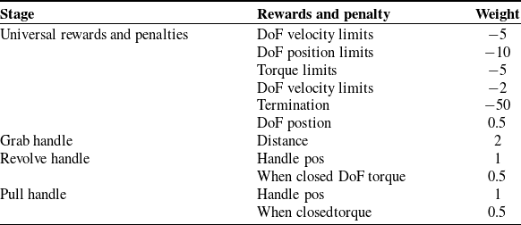
The above describes the special reward function design of the manipulator under different tasks. To guide the robotic agent towards safe and efficient task execution, we designed a set of universal and task-specific rewards and penalties, as summarized in Table II. Universal penalties are imposed for exceeding velocity, position, and torque limits of the robot joints (DoF: degree of freedom). For instance, exceeding the DoF position limit incurs a penalty of −10 per occurrence, while exceeding velocity or torque limits results in penalties of −5 and −2, respectively. These terms ensure the manipulator operates within safe mechanical bounds. Termination penalty: a significant negative reward of −50 is assigned for episode termination due to one of the following events: (1) task timeout (the agent does not complete the task within the allowed step limit), (2) collision with the environment (e.g., door, frame), and (3) manual emergency stop triggered for safety. Minimal positive reward (e.g., +0.5) is given for simply maintaining joint positions within safe ranges, which encourages stable control even when not making dramatic progress. The magnitude of each reward/penalty term has been empirically tuned to balance task completion, motion safety, and learning efficiency. The combination of these terms ensures the policy learns to maximize task progress while strictly avoiding unsafe behaviors.
Reward terms for pretraining.

5. Experiments
5.1. Simulation experiment of robotic arm lifting objects
In the virtual simulation experiments, we adopted three main performance parameters to evaluate and compare the proposed SAC-GP algorithm with the baseline SAC algorithm in the block grasping task: (1) convergence speed: defined as the number of training episodes required for the model’s reward curve to stabilize and reach a plateau; (2) average episode reward: the mean final reward achieved per episode, reflecting the policy’s effectiveness in completing the task and adhering to safety or efficiency objectives; and (3) robustness (reward fluctuation): quantified by the amplitude and frequency of reward fluctuations throughout training, indicative of the algorithm’s stability.
First, in the virtual environment, the block grasping experiment of the robotic arm was carried out to compare the SAC algorithm and the SAC-GP algorithm. The hyperparameters of the algorithms are shown in Table III.
Hyperparameters of the “Lift” simulation experiment algorithm.

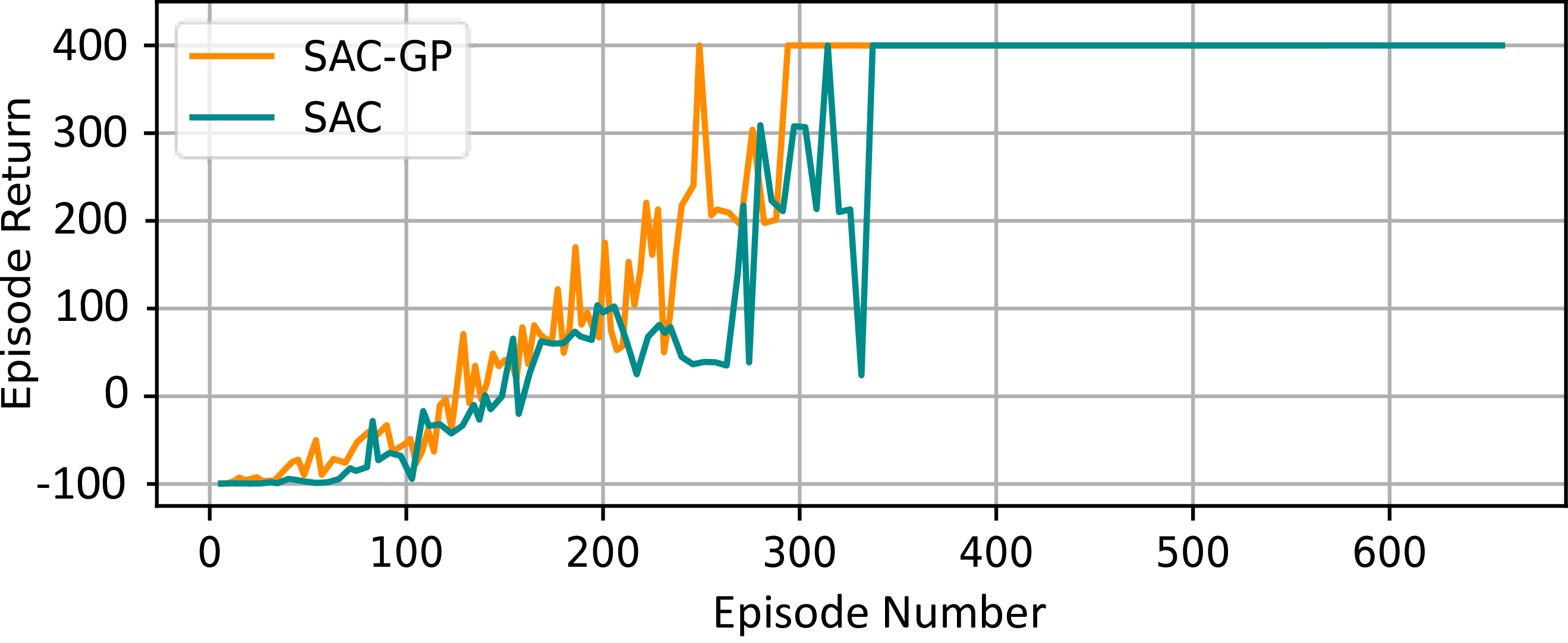
Figure 5 shows the training reward curve using the SAC-GP algorithm, and Figure 6 presents a direct comparison between SAC-GP and SAC. As can be seen, the SAC-GP algorithm achieves faster convergence, with the model stabilizing in about 300 episodes, whereas SAC requires approximately 330 episodes to converge. Additionally, the average episode reward attained by SAC-GP is consistently higher than that of SAC. Regarding robustness, the reward curve of SAC-GP exhibits notably fewer and smaller fluctuations compared to that of SAC, indicating greater training stability and robustness of the learned policy.
The training results of the block lifting experiment of the SAC-GP algorithm.

Comparison of the SAC-GP algorithm and the SAC algorithm in the “Lift” experiment.

These results demonstrate that the proposed SAC-GP algorithm not only achieves higher learning efficiency but also exhibits superior effectiveness and robustness compared to the baseline SAC algorithm.
5.2. Simulation experiment of robotic arm opening the door
The experiment introduces a hierarchical RL approach [Reference Liu, Wang, Liu, Liu, Liu and Huang33–Reference Tan, Fang, Zhang, Song, Chen, Zheng and Li36] to slice the complex task of robotic door-opening. Specifically, the door-opening task is divided into three subtasks: the first subtask is for the robotic arm to grasp the door handle, the second subtask is for the robotic arm to rotate the door handle, and the third task is for the robotic arm to pull the door handle. The adjusted hyperparameters for this experiment are shown in Table IV.
Hyperparameters of the “Door” simulation experiment algorithm.

Furthermore, this study also employs training acceleration techniques based on hierarchical RL [Reference Gupta, Yu, Zhao, Kumar, Rovinsky, Xu, Devlin and Levine37], achieving fully automatic scene initialization without manual intervention, thus speeding up the training process. To address the coupling relationship between subtasks, this paper defines the scene transition relationship for subtask training, as illustrated in Figure 7. The training starts with grasping the door handle. If the door handle is not successfully grasped, the training will continue with grasping the door handle; if the door handle is successfully grasped, the training will proceed to rotating the door handle; if the door handle is successfully rotated open, the training will then move on to pulling the door open. This process continues until the robotic arm successfully completes three subtasks, which are grabbing the door handle, rotating the door handle, and opening the door.
Subtask coupling relationship.

To quantitatively evaluate the performance of the proposed system, the following performance parameters are used: success rate: the proportion of episodes in which the robot successfully completes three subtasks and opens the door; average completion time: the average number of time steps or real time required to complete the door-opening task from start to finish; average reward: the mean cumulative reward accumulated by the agent per episode, reflecting both task efficiency and behavior quality; convergence episodes: the number of training episodes required for the policy to converge to a stable or near-optimal success rate; and robustness: the consistency of task completion under environmental perturbations or variations, such as noise, different initial positions, or changing door properties. These metrics provide a comprehensive assessment of the effectiveness, efficiency, and reliability of the proposed hierarchical RL approach for robotic door-opening.
5.2.1. Simulation experiment of robotic arm grabbing the door handle
Using the hyperparameters listed in Table IV and the SAC-GP algorithm, we conducted training on the door-grasping task. The change in reward and the number of steps per episode are shown in Figure 8. Similarly, training results with the original SAC algorithm are shown in Figure 9.
The reward curve obtained by the SAC-GP algorithm in the simulation experiment of the robotic arm grabbing the door handle.

The reward curve obtained by the SAC algorithm in the simulation experiment of the robotic arm grabbing the door handle.

Comparison results are summarized as follows: Convergence speed: The SAC-GP algorithm enables the agent to converge to an effective policy in approximately 130 episodes, while the original SAC algorithm requires around 210 episodes to achieve a similar level of performance, indicating faster learning with SAC-GP. Stability: In the stable phase, the reward curve of the SAC-GP agent exhibits 10 significant fluctuations, whereas the SAC agent’s reward curve has 12. This demonstrates improved stability with SAC-GP. Overall performance: The SAC-GP agent attains a higher average reward per episode and a higher final success rate, showing improved effectiveness for the door-opening task. These performance parameters comprehensively demonstrate that the SAC-GP algorithm provides superior efficiency and stability compared to the classical SAC algorithm in robotic door-opening tasks.
5.2.2. Simulation experiment of robotic arm revolving the door handle
Later, the revolving door handle was trained, and the change in reward value and round steps was shown in Figure 10. When training with the SAC algorithm, the changes in reward values and episode steps are illustrated in Figure 11.
The reward curve obtained by using the SAC-GP algorithm in the simulation experiment of the robotic arm revolving the door handle.

The reward curve obtained by using the SAC algorithm in the simulation experiment of the robotic arm rotating the doorknob.

Based on the predefined performance parameters, a comparative analysis between the SAC-GP and SAC algorithms yields the following insights: The SAC-GP algorithm achieves policy convergence in approximately 20 episodes, whereas the SAC algorithm requires about 40 episodes. This highlights the superior learning efficiency of SAC-GP. Stability: The reward curve of SAC-GP shows fewer significant fluctuations compared to that of SAC, indicating improved training stability and more consistent policy performance. Average reward: After convergence, the average cumulative reward per episode achieved by the SAC-GP algorithm is higher than that of the SAC algorithm, reflecting better overall task performance. In summary, with respect to the defined performance parameters – convergence speed, stability, and average reward – the SAC-GP algorithm demonstrates clear advantages over the original SAC algorithm for the robotic door-opening task.
5.2.3. Simulation experiment of robotic arm pulling the door handle
Finally, the change in reward values and episode steps during the door handle pulling training is shown in Figure 12. For comparison, the training results using the SAC algorithm are illustrated in Figure 13.
The reward curve obtained by using the SAC-GP algorithm in the simulation experiment of the robotic arm pulling the doorknob.

The reward curve obtained by using the SAC algorithm in the simulation experiment of the robotic arm pulling the door handle.

Based on the predefined performance parameters, a comparative analysis between the SAC-GP and SAC algorithms yields the following conclusions: the SAC-GP algorithm enables the agent to converge to an effective policy in approximately 40 episodes, whereas the SAC algorithm requires about 60 episodes to achieve a similar level of performance. This demonstrates the faster learning capability of SAC-GP. Stability: During training, the reward curve of the SAC-GP algorithm exhibits only two significant fluctuations, compared to four fluctuations observed with the SAC algorithm. This indicates that the SAC-GP algorithm achieves more stable training and policy performance. In summary, with respect to convergence speed and stability, the SAC-GP algorithm again demonstrates clear advantages over the original SAC algorithm for the door handle pulling subtask.
Across all three subtasks, the SAC-GP algorithm consistently achieves a better balance between exploration and exploitation, resulting in faster and more effective policy learning. Additionally, it demonstrates greater training stability, as evidenced by fewer significant fluctuations in the reward curves compared to the SAC algorithm. Collectively, these results demonstrate that SAC-GP outperforms the standard SAC algorithm in terms of both learning efficiency and stability for the robotic door-opening task. These advantages, reflected in the key performance metrics of convergence episodes and reward stability, confirm the overall superiority of the SAC-GP algorithm across all subtasks.
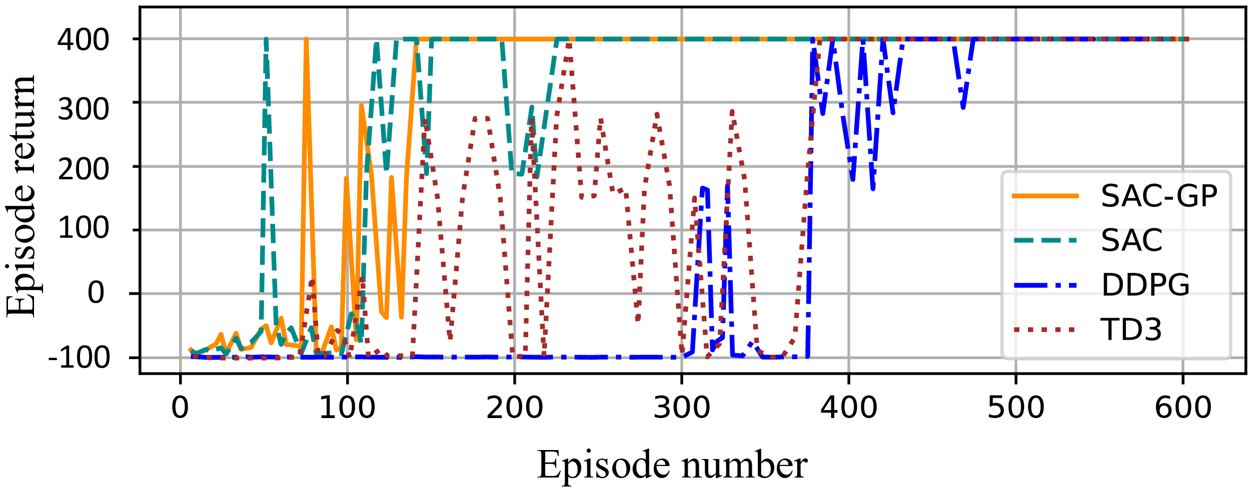
The SAC-GP algorithm proposed in this paper aims to address specific issues in the field of RL. To further evaluate the performance of the SAC-GP algorithm, comparative experiments were conducted with popular algorithms such as SAC, deep deterministic policy gradient (DDPG), and twin-delayed DDPG (TD3). These algorithms were used to perform door handle grasping experiments, and the experimental results are shown.
Comparison of the reward curves of RL algorithm in the experiment of grabbing doorknobs.

The SAC-GP algorithm proposed in this paper aims to address specific challenges in RL. To further evaluate its performance, comparative experiments were conducted against several popular algorithms, including SAC, DDPG, and TD3. These algorithms were each applied to the door handle grasping task, and the corresponding experimental results are presented in Figure 14. As shown in the figure, the SAC-GP algorithm not only achieves faster convergence to higher reward values during training but also maintains stable performance during testing. This suggests that SAC-GP achieves a more effective balance between exploration and exploitation, resulting in improved learning efficiency and performance. Overall, the experimental results on multiple benchmark tasks consistently demonstrate the superior performance of the SAC-GP algorithm. The comparative evaluation with other state-of-the-art algorithms further confirms its effectiveness and practical value in RL applications.
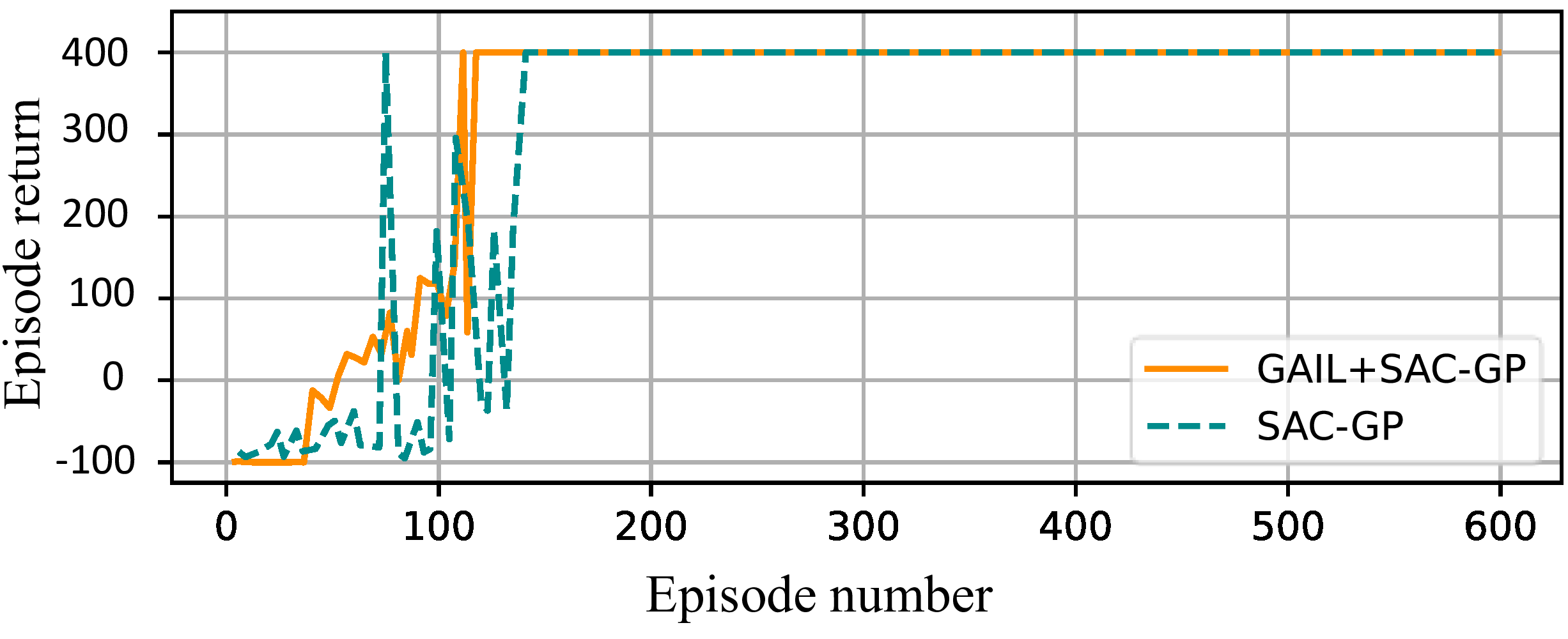
In addition, experiments were conducted in the MuJoCo + RoboSuite simulation environment, where a robotic arm was tasked with grasping a door handle. The reward curves for the GAIL + SAC-GP algorithm and the SAC-GP algorithm are shown in Figure 15 for comparison. From these results, it is evident that combining the GAIL algorithm with SAC-GP significantly accelerates the convergence of training and achieves greater stability compared to using SAC-GP alone. This demonstrates the enhanced effectiveness of the GAIL + SAC-GP algorithm for the robotic door handle grasping task.
Comparison of reward curves between GAIL + SAC-GP algorithm and SAC-GP algorithm.

5.3. Experiments in a real-world environment
In the field of robotics, it is a highly effective method to first train agents in a virtual environment and then apply them to real-world environments through Sim2Real. The control strategies learned by the agent in the virtual environment can be directly applied to the real-world environment or fine-tuned in the real-world environment to adapt to environmental differences.
In this study, the agent was first pretrained in a virtual environment. Then, through Sim2Real [Reference Zhu, Lin, Jain and Zhou28–Reference Sandha, Garcia, Balaji, Anwar and Srivastava32], the policy network trained in the virtual environment was transplanted to the real-world environment, followed by fine-tuning and optimization of the transferred policy network.
Rigid body models such as grippers and door handles were created in the motion capture software, with the positions of the reflective markers attached as shown in Figure 16. The capture effect within the motion capture software is illustrated in Figure 17.
Position of attaching reflective targets such as grippers and door handles.

5.3.1. Robot arm grasping door handle experiment
A total of 30 sets of door handle grasping experiments were conducted to test the reliability of the trained model, and the operation success rate was calculated as shown in Table V.
In the 30 sets of robot arm grasping door handle experiments, the robot arm was initialized to different positions within the operational space, and the grasping success rate was
 $ 97\%$
. Among the failed cases, the claw knocked off the reflective target ball on the door handle, resulting in a failed grasp. Therefore, it can be concluded that the experiment has achieved relatively satisfactory results.
One set of successful experimental data was selected for result analysis, and the actual trajectory of the end point position was collected, as shown in Figure 18.
Statistics of the success rate of the robotic arm grabbing the doorknob.

Software recognition result under the motion capture camera.

The actual running track of the end point of the manipulator grabbing the door handle.

5.3.2. Robotic arm revolving door handle experiment
A total of 30 sets of rotating door handle experiments were conducted to test the reliability of the model. The task success rate was counted and calculated, as shown in Table VI.
In the 30 sets of robot arm rotating door handle experiments, the pose after successfully grasping the door handle from different positions within the operational space was used as the initial state for each set of experiments. The success rate of rotating the door handle reached
 $ 93.3\%$
, achieving good results. Among the failed cases, one was due to the claw detaching from the door handle, and the other was caused by the claw not rotating the door handle to a sufficient angle to fully unlock the lock. Overall, the experiment has achieved relatively satisfactory results.
Statistics of the success rate of robotic arm revolving door handles.

One set of model test data was selected for analysis, and the actual trajectory of the target object was obtained, as shown in Figures 19 and 20.
Trajectory of the end-effector of the robotic arm in the X Y Z spatial coordinate system.

5.3.3. Robotic arm pulling door handle experiment
A total of 30 sets of door handle pulling experiments were conducted to test the reliability of the model. The task success rate was counted and calculated, as shown in Table VII.
In the 30 sets of experiments on door handle pulling using a robotic arm, each set of experiments used different positions in the operating space of the robotic arm to grasp the door handle and rotate the door handle’s pose as the initial state. The success rate of pulling the door open reached
 $ 96.7\%$
, achieving good results. Among them, the cases of failure were as follows: the gripper detached from the door handle during the process of pulling the door handle, but the door was already open. As shown in Table VII, the experiment has achieved relatively ideal results.
Statistics on the success rate of the manipulator pulling door handles.

Trajectory of the end-effector of the robotic arm within the X Y plane.

Trajectory of the end-effector of the robotic arm in the X Y Z spatial coordinate system.

A set of model test data was selected for analysis to obtain the actual running trajectory of the target object, as shown in Figures 21 and 22.
Trajectory of the end-effector of the robotic arm within the X Y plane.

5.3.4. Robotic arm door-opening experiment
Based on the tasks of “grasping the door handle,” “rotating the door handle,” and “pulling the door handle,” this experiment conducted a “robotic arm door opening” experiment. The models trained from the first three tasks were used as “basic action” models for “skill stitching,” enabling the agent to complete the door-opening task in its entirety, as shown in Figure 23.
Experimental process of the robotic arm door-opening task.

6. Conclusion
This paper designs and constructs a robotic arm learning system based on multi-source sensor information fusion. By integrating multi-source sensor information and combining demonstration learning with DRL algorithms, the system has successfully transformed human teaching data into empirical strategies for the robotic arm to perform tasks. It has also successfully transferred the agent trained in a virtual environment to the real environment through Sim2Real and completed predefined, complex tasks in the real environment. The main research achievements of this paper are reflected in: robotic arm task modeling and algorithm framework selection; establishing simulation experiments and real experimental environments; implementation, optimization, and experimentation of robotic arm learning algorithms in simulation environments; migrating the well-trained agent from simulation experiments to real environments; and conducting experimental verification.
While this paper has achieved certain results in DRL, demonstration learning, and Sim2Real, there are still several aspects that require further exploration and in-depth research:
-
1. Algorithm optimization and performance improvement: Although the current system can already complete complex tasks, future research can further improve and optimize the algorithms to enhance the robotic arm’s adaptability and robustness in complex environments.
-
2. Expanding application scenarios: This study mainly focuses on the learning and application of robotic arms in specific tasks. In the future, the system can be applied to a wider range of scenarios, such as home service robots, and combined with large language models (LLM) to fully leverage its capabilities for autonomous learning and adaptation to complex environments. In particular, future work will focus on improving human–robot collaboration by planning robot movements that are aware of human intentions and needs. For example, in door handle manipulation tasks, the robotic arm will be equipped with intention recognition modules and adaptive planning strategies, enabling it to anticipate human actions and synergistically collaborate with humans. Specifically, by training vision-language-action (VLA) models, the robotic arm can better understand and interpret human intentions from multimodal inputs, further enhancing the efficiency, safety, and naturalness of human–robot interaction.
-
3. Enhancing human–robot interaction and collaboration: In a human–robot collaborative environment, the robotic arm needs to better interact and collaborate with humans. Future research can explore how to enhance the robotic arm’s perception and understanding capabilities to enable more natural communication and cooperation with humans.
-
4. Research on multimodal learning: In addition to spatial position and force information, other modal information (such as sound, touch, etc.) can be explored to enrich the robotic arm’s perceptual abilities, further improving its learning efficiency and task execution accuracy. Through continuous optimization of algorithms, expansion of application scenarios, and enhancement of human–robot interaction and collaboration, it is believed that the autonomous learning capabilities of robotic arms will be further improved in the future, bringing more convenience and benefits to human production and life.
Funding
This research was supported by the National Key Research and Development Program of China (2022YFB4700501).
Competing interests
The authors have no relevant financial or non-financial interests to disclose.
Data availability and access
Data are contained within the article.
Ethical and informed consent for data used
Not applicable.
Consent for publication
Not applicable.
Authors contribution
Conceptualization: Ze Cui; Methodology: Chenzhao Sun; Software and validation: Jingao Huang, Yang Zhang, and Zhenghao Chen; Writing – original draft preparation: Chenzhao Sun; Writing – review and editing: Ze Cui and Zhenghao Chen; Supervision: Ze Cui. All authors have read and agreed to the published version of the manuscript.