1 Introduction
A hydrodynamic Taylor–Couette flow with rotation profiles beyond the Rayleigh limit is stable against axi- and non-axisymmetric perturbations. It is unstable, however, against axisymmetric perturbations under the presence of axial magnetic background fields (Velikhov Reference Velikhov1959; Ji, Goodman & Kageyama Reference Ji, Goodman and Kageyama2001; Rüdiger & Zhang Reference Rüdiger and Zhang2001)) and it is unstable against non-axisymmetric perturbations under the presence of azimuthal fields (Tayler Reference Tayler1957; Ogilvie & Pringle Reference Ogilvie and Pringle1996). For axial fields and given magnetic Prandtl number
 $$\begin{eqnarray}\text{Pm}=\frac{\unicode[STIX]{x1D708}}{\unicode[STIX]{x1D702}}\end{eqnarray}$$
(with molecular viscosity
 $\unicode[STIX]{x1D708}$
and magnetic resistivity
 $\unicode[STIX]{x1D702}$
) there exists always a critical magnetic field amplitude with a minimal Reynolds number. These numbers are running with
 $1/\text{Pm}$
so that for the small magnetic Prandtl numbers of liquid metals the critical Reynolds numbers basically exceed values of
 $10^{6}$
(Rüdiger & Shalybkov Reference Rüdiger and Shalybkov2001). This very high Reynolds number is the main reason that to date the standard magnetorotational instability has not yet been realized in laboratory experiments.
For much lower critical Reynolds numbers the Couette flow becomes unstable if the magnetic background field is toroidal or has a toroidal component. Herron & Soliman (Reference Herron and Soliman2006) demonstrated that all flows with negative shear and current-free background fields are stable against axisymmetric perturbations. There and also here the flows are assumed as unbounded in the axial direction. The existing instabilities must thus always be non-axisymmetric. For the absolutely lowest possible magnetic field amplitude, the critical Reynolds number for the onset of this so-called azimuthal magnetorotational instability (AMRI) for liquid metals such as gallium or sodium is only
 $O(10^{3})$
, hence there is a very strong reduction compared with the Reynolds numbers needed for the magnetorotational instability with axial fields. Not surprisingly, the AMRI at and slightly beyond the Rayleigh line has already been realized in the laboratory (Seilmayer et al.
Reference Seilmayer, Galindo, Gerbeth, Gundrum, Stefani, Gellert, Rüdiger, Schultz and Hollerbach2014).
The non-axisymmetric AMRI also exists for flows rotating with a positive shear
 $\text{d}\unicode[STIX]{x1D6FA}/\text{d}R$
(‘super-rotation’). This is of relevance insofar as super-rotating Taylor–Couette flows are prototypes of very stable hydrodynamic flows (but see Deguchi (Reference Deguchi2017) for a non-axisymmetric instability at high Reynolds numbers). For conducting fluids with magnetic Prandtl numbers less or larger than unity (excluding
 $\text{Pm}=1$
) such flows can easily be destabilized with supercritical toroidal magnetic fields. The needed Reynolds numbers (of the outer cylinder) for flows with stationary inner cylinder are only
 $O$
(100), see Stefani & Kirillov (Reference Stefani and Kirillov2015) and Rüdiger et al. (Reference Rüdiger, Gellert, Hollerbach, Schultz and Stefani2018).
Another instability exists for conducting fluids wherein axial electric currents produce azimuthal magnetic fields with radial profiles less steep than the vacuum profile
 $1/R$
where
 $R$
is the radius in cylindric coordinates. The relation
 $$\begin{eqnarray}\frac{\text{d}}{\text{d}R}(RB_{\unicode[STIX]{x1D719}}^{2})\leqslant 0\end{eqnarray}$$
is a sufficient and necessary condition for stability of a stationary ideal fluid against non-axisymmetric perturbations (Tayler Reference Tayler1973). One finds instability in particular for the azimuthal field with the radial profile
 $B_{\unicode[STIX]{x1D719}}\propto R$
produced by a uniform electric current. The existence of a non-axisymmetric instability for such a (non-rotating)
 $z$
-pinch has been shown by Seilmayer et al. (Reference Seilmayer, Stefani, Gundrum, Weier, Gerbeth, Gellert and Rüdiger2012) using the liquid GaInSn alloy as the conducting fluid penetrated by an axial electric current of
 $\simeq 3$
kAmp.
The combination of a current-free magnetic field
 $B_{\unicode[STIX]{x1D719}}\propto 1/R$
and the rotation profile
 $\unicode[STIX]{x1D6FA}\propto 1/R^{2}$
of the potential flow belongs to a particular class of magnetohydrodynamical flows defined by the condition that the factor
 $\text{Mm}$
(the magnetic Mach number) in the relation
 $$\begin{eqnarray}\boldsymbol{U}=\text{Mm}~\boldsymbol{U}_{\text{A}},\end{eqnarray}$$
with
 $\boldsymbol{U}$
the flow velocity and
 $\boldsymbol{U}_{\text{A}}=\boldsymbol{B}/\sqrt{\unicode[STIX]{x1D707}_{0}\unicode[STIX]{x1D70C}}$
its Alfvén speed, is a constant value (Chandrasekhar Reference Chandrasekhar1956; Tataronis & Mond Reference Tataronis and Mond1987). Applied to Taylor–Couette flows unbounded in axial direction the radial profiles of the flow velocity
 $U_{\unicode[STIX]{x1D719}}$
and
 $B_{\unicode[STIX]{x1D719}}$
are required to be identical. All such flows are stable in the absence of diffusive effects. On the other hand, it is known that the (Chandrasekhar-type) potential flow of real fluids with
 $\unicode[STIX]{x1D6FA}\propto 1/R^{2}$
can easily be destabilized by a current-free toroidal magnetic field with
 $B_{\unicode[STIX]{x1D719}}\propto 1/R$
(Rüdiger et al.
Reference Rüdiger, Hollerbach, Schultz and Elstner2007). All these magnetized flows possess neutral stability for certain maximal Reynolds numbers for fixed Hartmann number, where these values do not depend on
 $\text{Pm}$
for
 $\text{Pm}\rightarrow 0$
. Even in the inductionless approximation
 $\text{Pm}=0$
these eigenvalues remain finite. Another prominent example of Chandrasekhar-type flows is the rigidly rotating
 $z$
-pinch where the flow
 $U_{\unicode[STIX]{x1D719}}$
and the field
 $B_{\unicode[STIX]{x1D719}}$
are both proportionate to the cylinder radius
 $R$
.
The latter version of magnetized Taylor–Couette flows will be considered in the present paper to probe its qualification to transport angular momentum. In the cylinder coordinates used for Taylor–Couette flows (unbounded in
 $z$
) only the radial component
 $T_{R}$
of the total stress tensor must be considered which is formed by the (
 $R\unicode[STIX]{x1D719}$
) components of the difference of Reynolds stress and Maxwell stress. In the so-called diffusion approximation the
 $T_{R}$
component has been written as
 $$\begin{eqnarray}T_{R}=-\unicode[STIX]{x1D708}_{\text{T}}R\frac{\text{d}\unicode[STIX]{x1D6FA}}{\text{d}R},\end{eqnarray}$$
with positive eddy viscosity
 $\unicode[STIX]{x1D708}_{\text{T}}$
. Such a relation has originally been formulated for hydrodynamical turbulence (Boussinesq Reference Boussinesq1897) based on the observation that in a rigidly rotating fluid no angular momentum is transported. We shall see, however, that for the pinch-type instability the diffusion approximation (1.4) does not hold for uniform rotation. This gives a new possibility to estimate the magnetic-instability-induced turbulent viscosity for differentially rotating magnetized fluids. The resulting expression can also be considered as a confirmation of the viscosity approximation introduced by Shakura & Sunyaev (Reference Shakura and Sunyaev1973) and Pringle (Reference Pringle1981) to the accretion disk theory as an explanation of the angular momentum transport in thin disks.
Furthermore, some important applications of stellar physics are based on (1.4). We know from helioseismology that the solar radiative core rotates rigidly. One needs effective viscosities of
 $10^{4}$
times the molecular value to explain the decay of an initial rotation law within the lifetime of the Sun. Also the Maxwell stress theory of this decay needs an increase of the microscopic viscosity by a few orders of magnitude for the explanation of the rigid rotation of the solar interior (Charbonneau & MacGregor Reference Charbonneau and MacGregor1992; Rüdiger & Kitchatinov Reference Rüdiger and Kitchatinov1996). It remains to be tested whether the angular momentum transport by magnetic instabilities of fossil internal toroidal fields is strong enough to produce the quasi-uniform inner rotation of the Sun.
The lithium at the surface of cool main-sequence stars decays with a time scale of 1 Gyr. It is burned at temperatures in excess of
 $2.6\times 10^{6}$
K, which exists about 40.000 km below the base of the solar convection zone. There must be a diffusion process down to this layer of the burning temperature. A slow (!) transport process is needed which is one or two orders of magnitude faster than the molecular diffusion.
In this paper we mainly present the linear theory of rigidly rotating
 $z$
-pinches with a homogeneous axial electric current for two sorts of boundary conditions in order to calculate the instability-induced normalized radial transport of angular momentum. The basic equations of magnetohydrodynamics (MHD) are presented in § 2. The eigenfunctions of the unstable solutions and the instability-originated angular momentum transport (its ‘
 $\unicode[STIX]{x1D6EC}$
effect’) for given magnetic Prandtl number are presented in § 3. The transition to differential rotation also in terms of an eddy viscosity is discussed in § 4. Because of the importance of the Boussinesq relation (1.4) for the angular momentum transport in thin Kepler disks the stability of quasi-Keplerian rotation subject to azimuthal magnetic fields has been studied in more detail. Section 5 concludes the paper with a short discussion.
2 The equations
The equations of magnetic-instability theory are the well-known MHD equations
 $$\begin{eqnarray}\displaystyle \frac{\unicode[STIX]{x2202}\boldsymbol{U}}{\unicode[STIX]{x2202}t}+(\boldsymbol{U}\boldsymbol{\cdot }\unicode[STIX]{x1D735})\boldsymbol{U} & = & \displaystyle -\frac{1}{\unicode[STIX]{x1D70C}}\unicode[STIX]{x1D735}P+\unicode[STIX]{x1D708}\unicode[STIX]{x0394}\boldsymbol{U}+\frac{1}{\unicode[STIX]{x1D707}_{0}\unicode[STIX]{x1D70C}}\text{curl}\boldsymbol{B}\times \boldsymbol{B},\nonumber\\ \displaystyle \frac{\unicode[STIX]{x2202}\boldsymbol{B}}{\unicode[STIX]{x2202}t} & = & \displaystyle \text{curl}(\boldsymbol{U}\times \boldsymbol{B})+\unicode[STIX]{x1D702}\unicode[STIX]{x0394}\boldsymbol{B},\end{eqnarray}$$
with
 $\text{div}~\boldsymbol{U}=\text{div}~\boldsymbol{B}=0$
for an incompressible fluid;
 $\boldsymbol{U}$
is the velocity vector,
 $\boldsymbol{B}$
the magnetic field vector and
 $P$
the pressure. The basic state in the cylindric system with coordinates (
 $R,\unicode[STIX]{x1D719},z$
) is
 $U_{R}=U_{z}=B_{R}=B_{z}=0$
for the poloidal components and
 $$\begin{eqnarray}\unicode[STIX]{x1D6FA}=a+\frac{b}{R^{2}}\end{eqnarray}$$
for the rotation law with the constants
 $a=\unicode[STIX]{x1D6FA}_{\text{in}}(\unicode[STIX]{x1D707}-r_{\text{in}}^{2})/(1-r_{\text{in}}^{2})$
and
 $b=\unicode[STIX]{x1D6FA}_{\text{in}}R_{\text{in}}^{2}(1-\unicode[STIX]{x1D707})/(1-r_{\text{in}}^{2})$
. Here
 $r_{\text{in}}=R_{\text{in}}/R_{\text{out}}$
is the ratio of the inner cylinder radius
 $R_{\text{in}}$
and the outer cylinder radius
 $R_{\text{out}}$
;
 $\unicode[STIX]{x1D6FA}_{\text{in}}$
and
 $\unicode[STIX]{x1D6FA}_{\text{out}}$
are the angular velocities of the cylinders, respectively. With the definition
 $\unicode[STIX]{x1D707}=\unicode[STIX]{x1D6FA}_{\text{out}}/\unicode[STIX]{x1D6FA}_{\text{in}}$
, solid-body rotation with uniform
 $\unicode[STIX]{x1D6FA}$
is described by
 $\unicode[STIX]{x1D707}=1$
while
 $\unicode[STIX]{x1D707}<1$
belongs to rotation laws with negative radial shear (‘sub-rotation’). Super-rotation (positive shear,
 $\text{d}\unicode[STIX]{x1D6FA}/\text{d}R>0$
) leads to
 $\unicode[STIX]{x1D707}>1$
.
The stationary solution for the magnetic field which is current free in the fluid is
 $B_{\unicode[STIX]{x1D719}}=B_{\text{in}}R_{\text{in}}/R$
. We define
 $\unicode[STIX]{x1D707}_{B}=B_{\text{out}}/B_{\text{in}}$
, hence
 $\unicode[STIX]{x1D707}_{B}=r_{\text{in}}$
. For pinch-type solutions due to homogeneous axial electric currents with
 $B_{\unicode[STIX]{x1D719}}=B_{\text{in}}R/R_{\text{in}}$
it is
 $\unicode[STIX]{x1D707}_{B}=1/r_{\text{in}}$
.
The dimensionless physical parameters of the system besides the magnetic Prandtl number are the Hartmann number
 $\text{Ha}$
and the Reynolds number
 $\text{Re}$
,
 $$\begin{eqnarray}\displaystyle \text{Ha}=\frac{B_{\text{in}}D}{\sqrt{\unicode[STIX]{x1D707}_{0}\unicode[STIX]{x1D70C}\unicode[STIX]{x1D708}\unicode[STIX]{x1D702}}},\quad \text{Re}=\frac{\unicode[STIX]{x1D6FA}_{\text{in}}D^{2}}{\unicode[STIX]{x1D708}}. & & \displaystyle\end{eqnarray}$$
The magnetic Reynolds number is
 $\text{Rm}=\text{Pm}\cdot \text{Re}$
and the Lundquist number
 $\text{S}=\sqrt{\text{Pm}}\text{Ha}$
. The difference
 $D=R_{\text{out}}-R_{\text{in}}$
is the gap width between the cylinders. The Hartmann number is defined with the magnetic field at the inner wall. The ratio of the angular velocity of rotation and the Alfvén frequency of the magnetic field is the magnetic Mach number
 $\text{Mm}$
which can easily be expressed by the magnetic Reynolds number and the Lundquist number, i.e.
 $$\begin{eqnarray}\displaystyle \text{Mm}=\frac{\text{Rm}}{\text{S}}=\frac{\sqrt{\text{Pm}}\text{Re}}{\text{Ha}}. & & \displaystyle\end{eqnarray}$$
Fast rotation compared with the magnetic field is described by
 $\text{Mm}>1$
and slow rotation by
 $\text{Mm}<1$
;
 $\text{Mm}=1$
may be called a magnetic sonic point. Many cosmical objects can be characterized by
 $\text{Mm}>1$
with typical values of 10 for galaxies (Elstner, Beck & Gressel Reference Elstner, Beck and Gressel2014), approximately 1000 for the solar tachocline (when assuming a field of 1 kG) and for neutron stars with fields between
 $10^{15}$
G and
 $10^{12}$
G. The magnetic Mach number of White dwarfs reaches values of 600 becoming
 $\text{Mm}\gtrsim 1$
for the largest observed fields of 100 MG.
The variables
 $\boldsymbol{U}$
,
 $\boldsymbol{B}$
and
 $P$
are split into mean and fluctuating components, i.e.
 $\boldsymbol{U}=\bar{\boldsymbol{U}}+\boldsymbol{u}$
,
 $\boldsymbol{B}=\bar{\boldsymbol{B}}+\boldsymbol{b}$
and
 $P=\bar{P}+p$
. The bars from the mean-field variables are immediately dropped, so that from now on the capital letters
 $\boldsymbol{U}$
,
 $\boldsymbol{B}$
and
 $P$
represent the large-scale background quantities. Simplifying, the non-axisymmetric components of flow and field may be used in the following as the fluctuations while the axisymmetric components are considered as the mean quantities. Then the averaging procedure is the integration over the azimuth
 $\unicode[STIX]{x1D719}$
. By developing the fluctuations
 $\boldsymbol{u}$
,
 $\boldsymbol{b}$
and
 $p$
into normal modes,
 $[\boldsymbol{u},\boldsymbol{b},p]=[\boldsymbol{u}(R),\boldsymbol{b}(R),p(R)]\exp (\text{i}(\unicode[STIX]{x1D714}t+kz+m\unicode[STIX]{x1D719}))$
, the solutions of the linearized MHD equations are considered for axially unbounded cylinders. Here
 $k$
is the axial wavenumber of the perturbation,
 $m$
its azimuthal wavenumber and
 $\unicode[STIX]{x1D714}$
the complex frequency including growth rate as its negative imaginary part and a drift frequency
 $\unicode[STIX]{x1D714}_{\text{dr}}$
as its real part. A numerical code is used to solve the resulting set of linearized ordinary differential equations for the radial functions of flow, field and pressure fluctuations. The solutions are optimized with respect to the Reynolds number for given Hartmann number by varying the wavenumber. Only solutions for
 $|m|=1$
are here discussed. For consistency only such small Hartmann numbers are considered for which only these lowest unstable modes are excited.
2.1 Boundary conditions
The hydrodynamic boundary conditions at the cylinder walls are the rigid ones, i.e.
 $u_{R}=u_{\unicode[STIX]{x1D719}}=u_{z}=0$
. The cylinders are either considered as perfectly conducting or as insulating. For the conducting walls the fluctuations must fulfil
 $\text{d}b_{\unicode[STIX]{x1D719}}/\text{d}R+b_{\unicode[STIX]{x1D719}}/R=b_{R}=0$
at
 $R_{\text{in}}$
and
 $R_{\text{out}}$
so that ten boundary conditions exist for the set of ten differential equations. The magnetic boundary conditions for insulating walls are much more complicated, i.e.
 $$\begin{eqnarray}b_{R}+\frac{\text{i}b_{z}}{I_{m}(kR)}\left(\frac{m}{kR}I_{m}(kR)+I_{m+1}(kR)\right)=0,\end{eqnarray}$$
for
 $R=R_{\text{in}}$
and
 $$\begin{eqnarray}b_{R}+\frac{\text{i}b_{z}}{K_{m}(kR)}\left(\frac{m}{kR}K_{m}(kR)-K_{m+1}(kR)\right)=0,\end{eqnarray}$$
for
 $R=R_{\text{out}}$
, where
 $I_{m}$
and
 $K_{m}$
are modified Bessel functions of the second kind. The conditions for the toroidal field are simply
 $kRb_{\unicode[STIX]{x1D719}}=m\,b_{z}$
at
 $R_{\text{in}}$
and
 $R_{\text{out}}$
. More details including the modified expressions for cylinders with finite electric conductivity have been given by Rüdiger et al. (Reference Rüdiger, Gellert, Hollerbach, Schultz and Stefani2018).
For a magnetic field with
 $\unicode[STIX]{x1D707}_{B}=1/r_{\text{in}}$
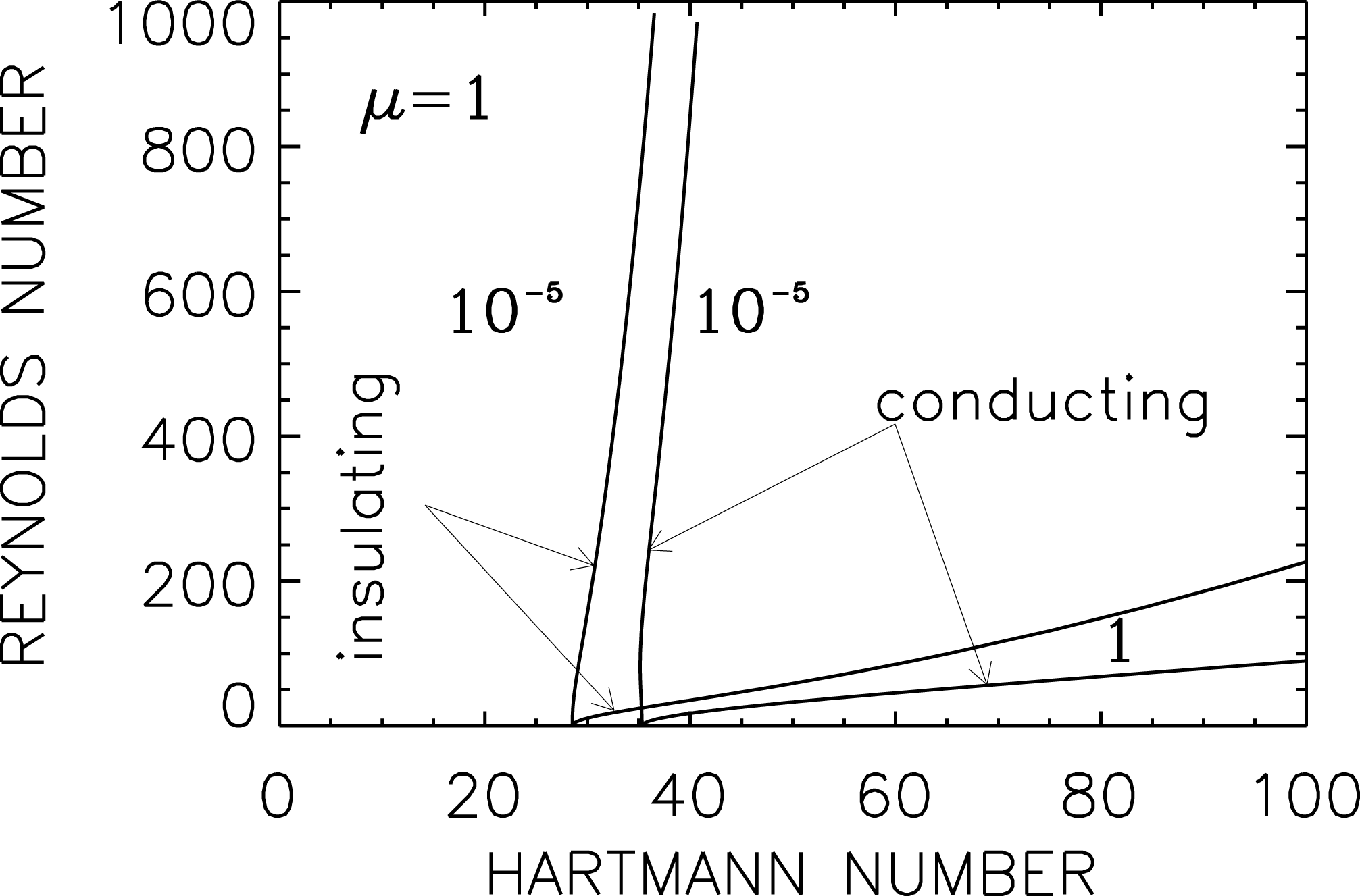
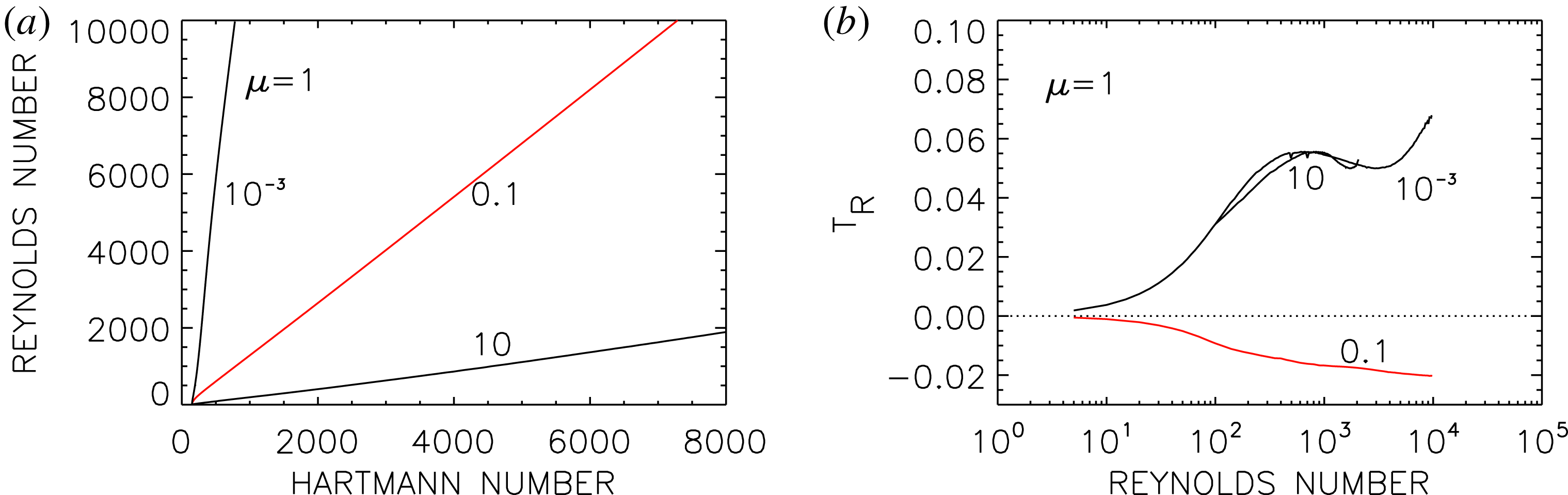
, figure 1 shows the lines of neutral stability (i.e. the maximal possible Reynolds number
 $\text{Re}_{\max }$
for fixed
 $\text{Ha}$
) for the rigidly rotating flow (
 $\unicode[STIX]{x1D707}=1$
). The Tayler instability for
 $m=\pm 1$
exists for not too weak fields and not too fast rotation. Absolute minima
 $\text{Ha}_{0}$
of the Hartmann numbers exist below which the fluid is stable. The curve of neutral instability limits the instability by suppressing the non-axisymmetric field mode by too fast rotation.
To demonstrate the influence of the boundary condition the figure 1 gives the instability lines for containers with perfectly conducting and insulating cylinders. The minimal Hartmann number for vacuum conditions (
 $\text{Ha}_{0}=28.1$
) proves to be smaller than the minimal Hartmann number for perfectly conducting conditions (
 $\text{Ha}_{0}=35.3$
). With insulating cylinders the magnetized Taylor–Couette flows become more easily unstable than with conducting cylinders.
Stability map
 $\text{Re}_{\max }=\text{Re}_{\max }(\text{Ha})$
for rigidly rotating
 $z$
-pinches with small and large magnetic Prandtl numbers (marked). Models with parameters below the lines are unstable. Boundary conditions: perfectly conducting cylinders as well as insulating cylinders.
 $\unicode[STIX]{x1D707}=1$
,
 $\unicode[STIX]{x1D707}_{B}=2$
,
 $r_{\text{in}}=0.5$
,
 $m=\pm 1$
.

As already noted the magnetized flow of figure 1 constitutes a standard example of the Chandrasekhar-type flows. The relations
 $\unicode[STIX]{x1D6FA}\propto R^{-q}$
and
 $B_{\unicode[STIX]{x1D719}}\propto R^{1-q}$
defining these flows in Taylor–Couette systems lead to the Chandrasekhar condition
 $$\begin{eqnarray}\unicode[STIX]{x1D707}=r_{\text{in}}\unicode[STIX]{x1D707}_{B},\end{eqnarray}$$
hence
 $\unicode[STIX]{x1D707}_{B}=2\unicode[STIX]{x1D707}$
for
 $r_{\text{in}}=0.5$
. This general condition is fulfilled for the rigidly rotating
 $z$
-pinch with
 $\unicode[STIX]{x1D707}=1$
and
 $\unicode[STIX]{x1D707}_{B}=2$
. The lines of marginal stability of the flow basically coincide in the (
 $\text{Ha}/\text{Re}$
) plane for
 $\text{Pm}\rightarrow 0$
. All curves for small
 $\text{Pm}$
in figure 1 are thus identical (and invisible).
The magnetic Prandtl number of
 $\text{Pm}=10^{-5}$
characterizes liquid sodium as the conducting fluid. The plotted lines of marginal instability are valid for all
 $\text{Pm}\leqslant 10^{-5}$
including
 $\text{Pm}=0$
. They thus can also be obtained by use of the inductionless approximation.
The
 $z$
-pinch is characterized by a homogeneous electric current in the axial direction which becomes unstable even without rotation if the current is strong enough. As is also demonstrated by the instability map, the numerical value of
 $\text{Ha}_{0}$
does (slightly) depend on the boundary conditions but does not depend on the magnetic Prandtl number. On the other hand, however, the rotational suppression of the Tayler instability strongly depends on the magnetic Prandtl number. For the very small
 $\text{Pm}$
it almost disappears. The curves in figure 1 can also be characterized by magnetic Mach numbers which are almost independent of the numerical value of the Hartmann number. Obviously the magnetic Mach number slightly exceeds unity for
 $\text{Pm}\simeq 1$
but it becomes smaller for smaller
 $\text{Pm}$
. As it is true for all Chandrasekhar-type flows (which scale with
 $\text{Ha}$
and
 $\text{Re}$
for
 $\text{Pm}\rightarrow 0$
) the magnetic Mach number decreases with decreasing
 $\sqrt{\text{Pm}}$
for very small
 $\text{Pm}$
which limits the astrophysical relevance of the instability for objects of small magnetic Prandtl number.
2.2 Angular momentum transport
It is known that the instability-induced radial angular momentum transport can be described with the (
 $R\unicode[STIX]{x1D719}$
) component of the total stress tensor,
 $$\begin{eqnarray}\unicode[STIX]{x1D61B}_{ij}=\langle u_{i}u_{j}\rangle -\frac{1}{\unicode[STIX]{x1D707}_{0}\unicode[STIX]{x1D70C}}\langle b_{i}b_{j}\rangle +\frac{1}{2\unicode[STIX]{x1D707}_{0}\unicode[STIX]{x1D70C}}\langle \boldsymbol{b}^{2}\rangle \unicode[STIX]{x1D6FF}_{ij},\end{eqnarray}$$
as the difference
 $$\begin{eqnarray}T_{R}=\langle u_{R}u_{\unicode[STIX]{x1D719}}\rangle -\frac{1}{\unicode[STIX]{x1D707}_{0}\unicode[STIX]{x1D70C}}\langle b_{R}b_{\unicode[STIX]{x1D719}}\rangle\end{eqnarray}$$
of the Reynolds and Maxwell stress tensor components taken at the same spatial and temporal coordinates. In the diffusion approximation (1.4) this expression is assumed to exist only for non-uniform rotation, representing angular momentum as flowing in the direction of slower rotation. To probe the applicability of the diffusion approximation we shall compute (2.9) for magnetic instabilities. As the Tayler instability even exists for rigid rotation its angular momentum transport should vanish. We shall calculate the radial flux of the angular momentum (2.9) along the lines of neutral stability where the rotation is maximal.
3 Rotating
 $z$
-pinches

The
 $z$
-pinch is formed by a uniform electric current throughout the entire region
 $R<R_{\text{out}}$
. Any resulting instability is purely current driven, it even exists for
 $\text{Re}=0$
and the rotation only suppresses (Pitts & Tayler Reference Pitts and Tayler1985). The curves of figure 1 demonstrate the stabilizing effect of rotation which is strongest for
 $\text{Pm}=1$
. It becomes weaker for smaller magnetic Prandtl numbers. In all cases a maximal Reynolds number
 $\text{Re}_{\max }$
exists for a given Hartmann number above which the
 $z$
-pinch is stable. The
 $\text{Re}_{\max }$
, defining the Reynolds number of neutral stability, depends on the magnetic Prandtl number, i.e. the smaller the
 $\text{Pm}$
the higher the
 $\text{Re}_{\max }$
. Quasi-Keplerian flow of
 $\text{Ha}=50$
allows instability only up to
 $\text{Re}_{\max }\simeq 1000$
for
 $\text{Pm}=1$
and
 $\text{Re}_{\max }\simeq 3000$
for
 $\text{Pm}=0.01$
independent of the used boundary conditions.
3.1 The eigenfunctions
The homogeneous system of differential equations for the perturbations forms an eigenvalue problem with eigensolutions for
 $\boldsymbol{u}(R)$
and
 $\boldsymbol{b}(R)$
which can be determined up to a free, real multiplication factor. The sign of products of two perturbation components remains unchanged. For the mode with
 $m=1$
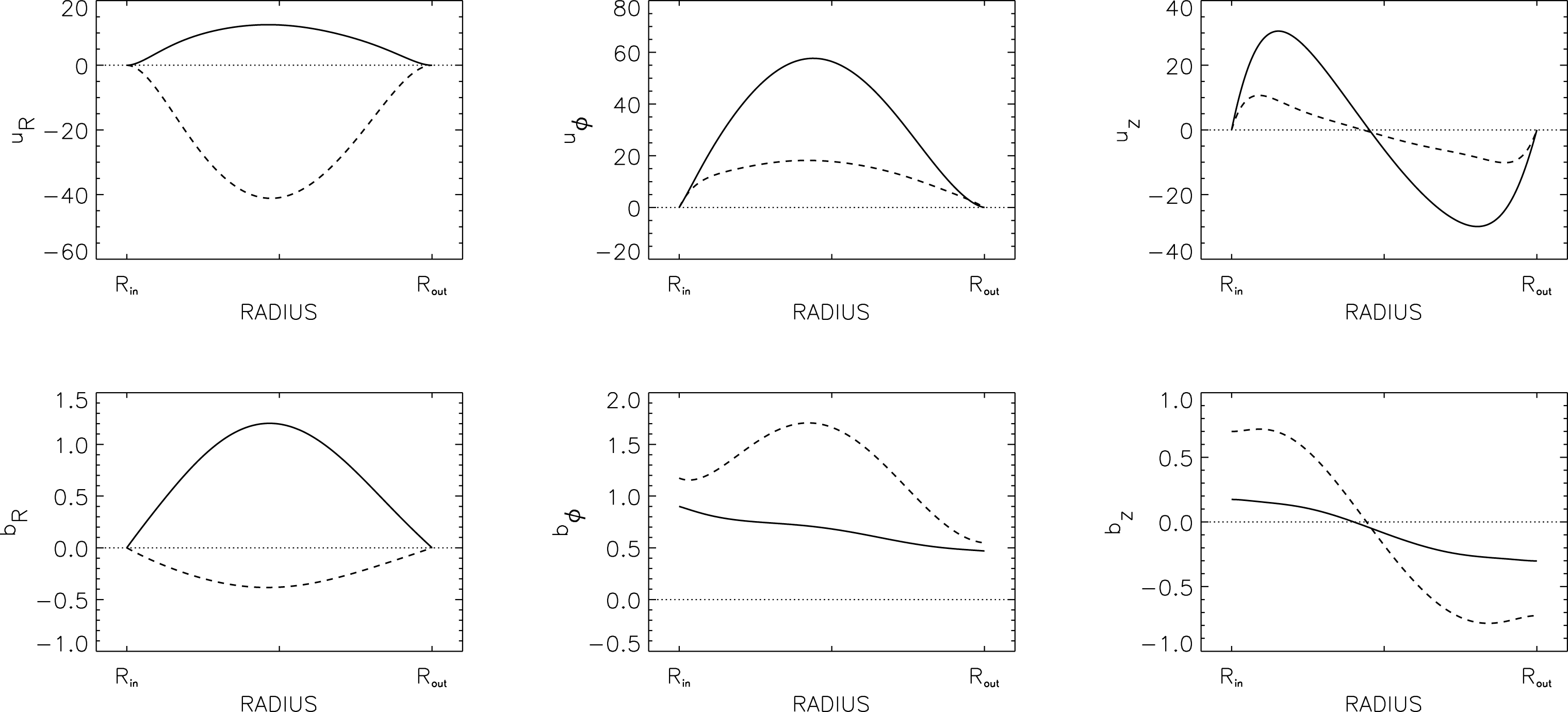
these functions in their dependence on
 $R$
are given in figure 2 for
 $\text{Pm}=0.1$
. Note the boundary conditions
 $\boldsymbol{u}=0$
and
 $b_{R}=0$
(for perfectly conducting walls) as fulfilled. One also finds, as one must, for
 $m=-1$
the components
 $u_{R},u_{\unicode[STIX]{x1D719}},b_{R}$
and
 $b_{\unicode[STIX]{x1D719}}$
are conjugate-complex as also the field components
 $-\text{i}u_{z}$
and
 $-\text{i}b_{z}$
are. This means that for the transformation
 $m\rightarrow -m$
the components
 $b_{R}$
transform as
 $b_{R}^{\text{R}}\rightarrow b_{R}^{\text{R}}$
and
 $b_{R}^{\text{I}}\rightarrow -b_{R}^{\text{I}}$
(the same for
 $b_{\unicode[STIX]{x1D719}}$
) while it is
 $b_{z}^{\text{R}}\rightarrow -b_{z}^{\text{R}}$
and
 $b_{z}^{\text{I}}\rightarrow b_{z}^{\text{I}}$
. The superscript R stands for the real part and I for the imaginary part of the eigensolutions.
The product of two scalars
 $A$
and
 $B$
after averaging over the
 $\unicode[STIX]{x1D719}$
coordinate is the sum of the products of the real parts and the imaginary parts, i.e.
 $AB=A^{\text{R}}B^{\text{R}}+A^{\text{I}}B^{\text{I}}$
. There is a certain factor in front of this expression whose value, however, is unimportant as in the linear theory the vector components are only known up to a free factor. In figure 2 the magnetic-induced contribution
 $b_{R}b_{\unicode[STIX]{x1D719}}$
to the radial flux of angular momentum is positive. One expects
 $b_{R}b_{\unicode[STIX]{x1D719}}\simeq 0$
for rigid rotation which, however, is here not the case. As the kinetic transport
 $u_{R}u_{\unicode[STIX]{x1D719}}$
is (slightly) negative the total stress component
 $T_{R}$
is negative, too.
Eigenfunctions (real parts: solid lines; imaginary parts: dashed lines) of the rigidly rotating
 $z$
-pinch for
 $\text{Ha}=50$
and
 $\text{Re}=144$
for perfectly conducting boundary conditions.
 $r_{\text{in}}=0.5$
.
 $m=1$
,
 $\text{Pm}=0.1$
,
 $\unicode[STIX]{x1D707}_{B}=2$
,
 $\unicode[STIX]{x1D707}=1$
.

The plotted amplitudes of the functions are completely arbitrary, they do not have a physical meaning. The above given sign rules for the products of the radial and azimuthal components of the flow and fields are not influenced by the boundary conditions. As with our normalizations the total stress results from the difference
 $\langle u_{R}u_{\unicode[STIX]{x1D719}}\rangle -\text{Pm}\text{Ha}^{2}\langle b_{R}b_{\unicode[STIX]{x1D719}}\rangle$
(where the instability sets in for almost constant
 $\text{Ha}$
if
 $\text{Pm}\rightarrow 0$
) the sign of the angular momentum transport is determined by the flow perturbations for small
 $\text{Pm}$
and by the magnetic fluctuations for large
 $\text{Pm}$
. The torque on the cylinders obviously vanishes if by the boundary conditions
 $u_{R}=b_{R}=0$
. The average procedure may concern the cylinder surface formed by
 $z$
and
 $\unicode[STIX]{x1D719}$
. Then it becomes
 $\langle u_{R}u_{\unicode[STIX]{x1D719}}\rangle \propto u_{R}^{\text{R}}u_{\unicode[STIX]{x1D719}}^{\text{R}}+u_{R}^{\text{I}}u_{\unicode[STIX]{x1D719}}^{\text{I}}$
. All the terms mixed in R and I disappear after averaging over the azimuth
 $\unicode[STIX]{x1D719}$
. The same procedure holds for the magnetic terms. From the transformation rules for
 $m\rightarrow -m$
it is clear that the modes
 $m$
and
 $-m$
lead to the same flux of angular momentum. The curves for
 $T_{R}$
in figure 3 are thus identical for
 $m=\pm 1$
.
We have to normalize the expression (2.9) in order to compensate the role of the free parameter in the eigenfunctions. To this end the
 $T_{R}$
is divided by the total energy
 $E=\langle \boldsymbol{u}^{2}\rangle +\langle \boldsymbol{b}^{2}\rangle /\unicode[STIX]{x1D707}_{0}\unicode[STIX]{x1D70C}$
(in our units
 $E=\langle \boldsymbol{u}^{2}\rangle +\text{Pm}\text{Ha}^{2}\langle \boldsymbol{b}^{2}\rangle$
). According to this definition the normalized
 $|T_{R}|$
should not exceed unity.
The angular momentum transport by the current-driven Tayler instability with
 $\unicode[STIX]{x1D707}_{B}=2$
and
 $\unicode[STIX]{x1D707}=1$
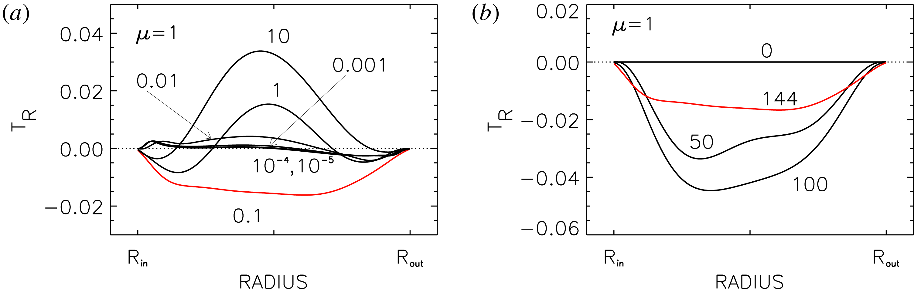
is given by figure 3 for a fixed Hartmann number,
 $\text{Ha}=50$
. The flow is of the Chandrasekhar-type and because of its uniform rotation, angular momentum should not be transported but it is. Note the negative value for
 $\text{Pm}\lesssim 0.1$
suggested above by inspection of figure 2. Generally, the transport direction depends on the magnetic Prandtl number, its absolute value
 $|T_{R}|$
becomes very small for the smallest magnetic Prandtl numbers. After (1.4) the angular momentum transport
 $T_{R}$
should vanish for all values of the parameters if the
 $z$
-pinch rotates with uniform
 $\unicode[STIX]{x1D6FA}$
, but this is not confirmed by the calculations.
Normalized angular momentum transport
 $T_{R}(R)$
for the
 $z$
-pinch with rigid rotation. (a) Variation of
 $\text{Pm}$
(marked) for neutral stability (
 $\text{Re}=\text{Re}_{\max }$
); (b) variation of
 $\text{Re}$
(marked) for fixed
 $\text{Pm}=0.1$
(vertical slice in the stability map). The curves are identical for
 $m\rightarrow -m$
.
 $\unicode[STIX]{x1D707}=1$
,
 $r_{\text{in}}=0.5$
,
 $\unicode[STIX]{x1D707}_{B}=2$
,
 $m=1$
,
 $\text{Ha}=50$
(always). Perfectly conducting boundary conditions.

3.2 The
$\unicode[STIX]{x1D6EC}$
effect for rigid-body rotation

Figure 3(a) gives the normalized radial fluxes of angular momentum between the two cylinders for the rigidly rotating
 $z$
-pinch for various magnetic Prandtl numbers and for one and the same (small) Hartmann number,
 $\text{Ha}=50$
and the maximal Reynolds number
 $\text{Re}_{\max }=144$
for
 $\text{Pm}=0.1$
. This flux is positive for large
 $\text{Pm}$
, it is negative for
 $\text{Pm}\lesssim 0.1$
and it almost vanishes for very small
 $\text{Pm}$
. As we know, for very small
 $\text{Pm}$
the angular momentum transport is dominated by the Reynolds stress. while for large
 $\text{Pm}$
the magnetic terms exceed the kinetic ones. Then the negativity of the Reynolds stress produces negative
 $T_{R}$
. For large magnetic Prandtl numbers this can be overcompensated by negative Maxwell stress
 $\langle b_{R}b_{\unicode[STIX]{x1D719}}\rangle$
. We note that there is no shear which could explain the anticorrelation of the fluctuations
 $b_{R}$
and
 $b_{\unicode[STIX]{x1D719}}$
.
Figure 3(b) demonstrates that the calculations along the line of neutral stability may underestimate the numerical values of the possible (normalized) angular momentum fluxes. The value of
 $T_{R}(R)$
is computed along a vertical slice for
 $\text{Ha}=50$
and
 $\text{Pm}=0.1$
. The growth rates of the instability pattern for these curves do not vanish. The curves are marked with the actual values of the Reynolds number. The red lines in both panels are identical. Of course,
 $T_{R}=0$
for
 $\text{Re}=0$
. The remaining curves for
 $\text{Re}=50$
and
 $\text{Re}=100$
yield larger numerical values as the curve for
 $\text{Re}=\text{Re}_{\max }$
.
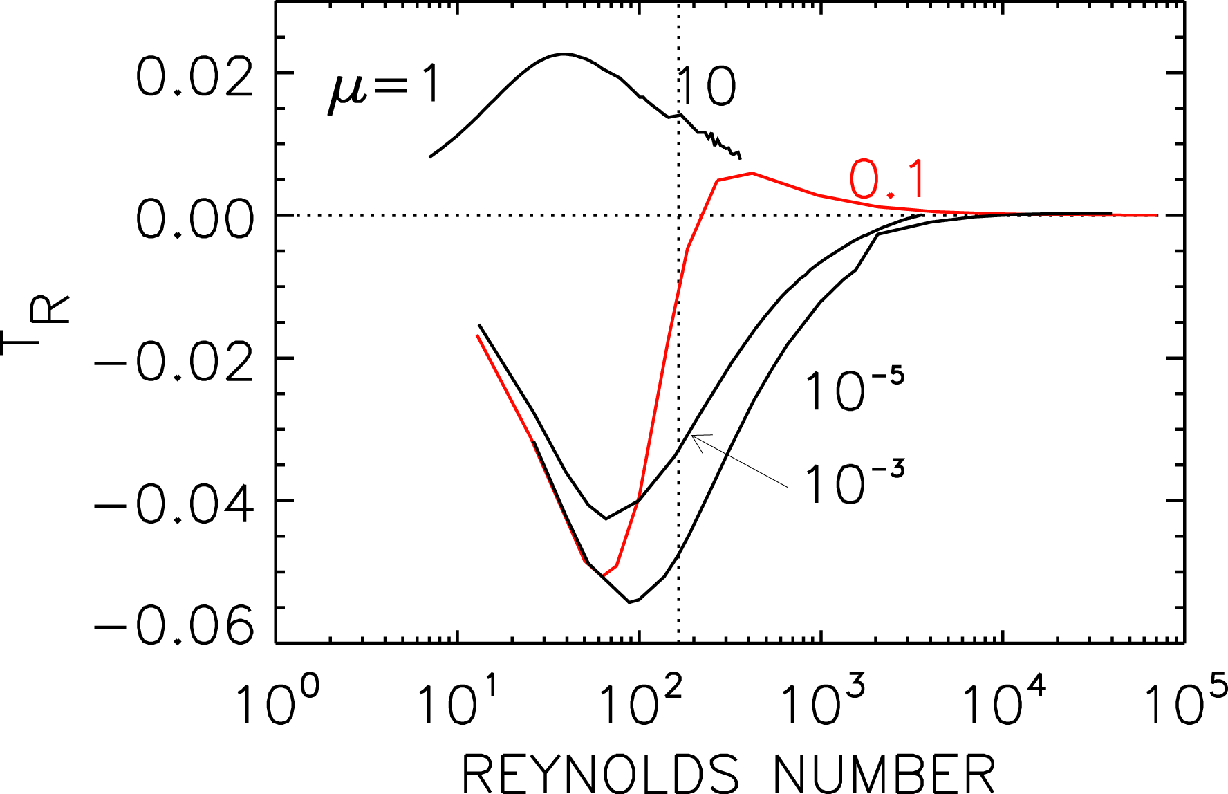
Figure 4 presents the normalized angular momentum transport
 $T_{R}$
for rigid rotation along the lines of neutral stability for several values of the magnetic Prandtl number. The value of
 $T_{R}$
is now averaged over the entire container. The vertical dotted line gives for
 $\text{Pm}=0.1$
the magnetic sonic point where
 $\text{Mm}=1$
. For the same
 $\text{Pm}$
the red line shows positive values for large magnetic Mach numbers and negative values for small magnetic Mach numbers. The graph also provides non-vanishing
 $T_{R}$
for
 $\text{Pm}\neq 0.1$
. For
 $\text{Pm}<0.1$
, even for faster rotation
 $T_{R}$
remains negative. For
 $\text{Pm}=10$
,
 $T_{R}$
is also finite but it is positive. The reason is that the magnetic sonic point for
 $\text{Pm}=10$
occurs already for
 $\text{Re}=13$
hence the main part of the corresponding curve belongs to super-Alfvénic flows. For
 $\text{Pm}=10^{-6}$
the magnetic sonic point is located at
 $\text{Re}\simeq 20.000$
.
Normalized and volume-averaged angular momentum transport
 $T_{R}$
for the rigidly rotating
 $z$
-pinch along the line of neutral instability (
 $\text{Re}=\text{Re}_{\max }$
). The curves are marked with
 $\text{Pm}$
. The momentum flux vanishes for
 $\text{Pm}=0.1$
close to the magnetic sonic point (the vertical dotted line). The curves are invariant against the transformation
 $m\rightarrow -m$
.
 $\unicode[STIX]{x1D707}=1$
,
 $\unicode[STIX]{x1D707}_{B}=2$
,
 $r_{\text{in}}=0.5$
,
 $m=\pm 1$
. Perfectly conducting boundary conditions.

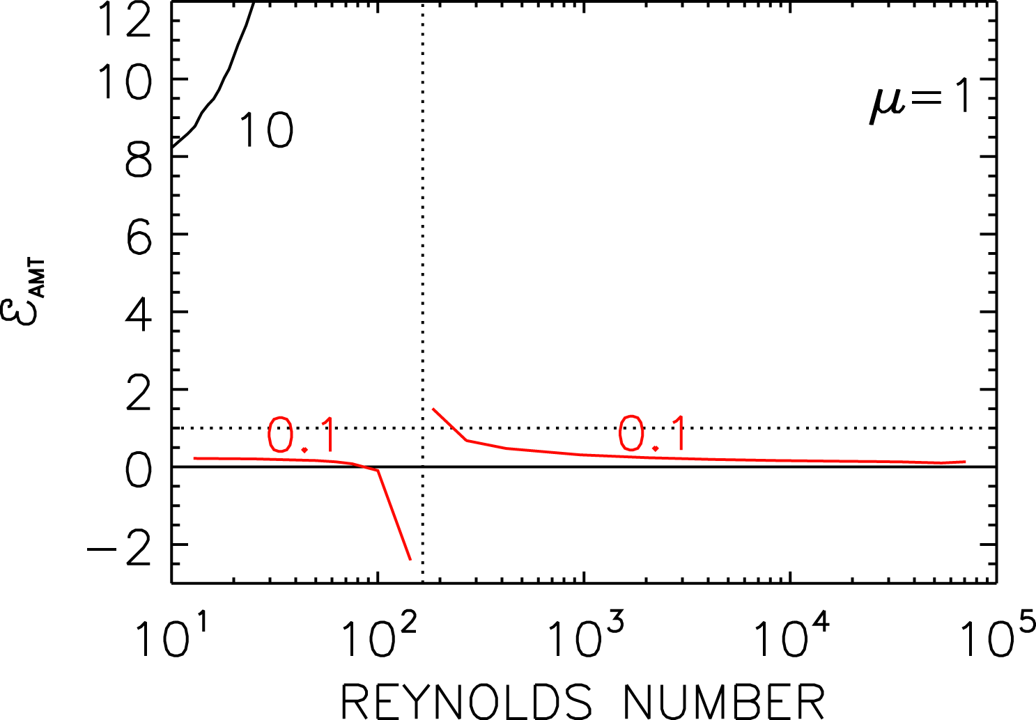
For a more detailed discussion figure 5 gives the ratio
 $$\begin{eqnarray}\unicode[STIX]{x1D700}_{\text{AMT}}=\frac{\langle b_{R}b_{\unicode[STIX]{x1D719}}\rangle }{\unicode[STIX]{x1D707}_{0}\unicode[STIX]{x1D70C}\langle u_{R}u_{\unicode[STIX]{x1D719}}\rangle }\end{eqnarray}$$
of the Maxwell stress and the Reynolds stress versus the Reynolds number for the containers with
 $\text{Pm}=0.1$
and
 $\text{Pm}=10$
. Striking differences only exist in the vicinity of the magnetic sonic point with
 $\text{Mm}=1$
(vertical dotted lines in figures 4 and 5). For larger as well as for smaller Reynolds numbers it is
 $0<\unicode[STIX]{x1D700}_{\text{AMT}}<1$
, hence the Reynolds stress (slightly) exceeds the Maxwell stress.
For the (normalized) stresses it is
 $$\begin{eqnarray}\langle u_{R}u_{\unicode[STIX]{x1D719}}\rangle \propto \frac{T_{R}}{1-\unicode[STIX]{x1D700}_{\text{AMT}}},\quad \frac{\langle b_{R}b_{\unicode[STIX]{x1D719}}\rangle }{\unicode[STIX]{x1D707}_{0}\unicode[STIX]{x1D70C}}\propto \unicode[STIX]{x1D700}_{\text{AMT}}\frac{T_{R}}{1-\unicode[STIX]{x1D700}_{\text{AMT}}}.\end{eqnarray}$$
For small
 $\unicode[STIX]{x1D700}_{\text{AMT}}>0$
it is
 $\langle u_{R}u_{\unicode[STIX]{x1D719}}\rangle \propto T_{R}$
and also
 $\langle b_{R}b_{\unicode[STIX]{x1D719}}\rangle \propto T_{R}$
. Both stresses possess the same sign. This case is realized along almost the whole red line of figure 5. Left from the vertical dotted line both stresses are negative and right from the dotted line both stresses are positive. A negative Maxwell stress for all sub-rotation laws is easy to understand via the induction process due to differential rotation but here it even exists for slow and rigid rotation. On the other hand, for large
 $|\unicode[STIX]{x1D700}_{\text{AMT}}|$
the Maxwell stress dominates and it is simply
 $\langle b_{R}b_{\unicode[STIX]{x1D719}}\rangle \simeq -T_{R}$
so that
 $\langle b_{R}b_{\unicode[STIX]{x1D719}}\rangle >0$
for
 $T_{R}<0$
(left from the dotted line) and
 $\langle b_{R}b_{\unicode[STIX]{x1D719}}\rangle <0$
for
 $T_{R}>0$
. The sign of the Maxwell stress changes where the red line crosses the horizontal solid line for
 $\unicode[STIX]{x1D700}_{\text{AMT}}=0$
.
Stress ratio (3.1) along the lines of neutral stability for
 $\text{Pm}=0.1$
and
 $\text{Pm}=10$
(averages over the container). The horizontal dotted line gives
 $\unicode[STIX]{x1D700}_{\text{AMT}}=1$
, the vertical line denotes the magnetic sonic point (
 $\text{Re}=180$
) for
 $\text{Pm}=0.1$
.
 $r_{\text{in}}=0.5$
,
 $\unicode[STIX]{x1D707}=1$
,
 $\unicode[STIX]{x1D707}_{B}=2$
,
 $m=1$
. Perfectly conducting boundary conditions.

The zeros of
 $T_{R}$
in figure 4 (horizontal dotted line) are defined by
 $\unicode[STIX]{x1D700}_{\text{AMT}}=1$
which happens close to the sonic point
 $\text{Mm}=1$
. For larger
 $\text{Mm}$
the Reynolds stress exceeds the Maxwell stress and it is positive leading to
 $T_{R}>0$
. For
 $\text{Mm}\simeq 1$
the magnetic stress becomes important and it is
 $\langle b_{R}b_{\unicode[STIX]{x1D719}}\rangle >0$
leading to negative
 $T_{R}$
. For even smaller Mach numbers again the Reynolds stress exceeds the Maxwell stress but both are now negative.
Large values
 $\unicode[STIX]{x1D700}_{\text{AMT}}>1$
for
 $\text{Pm}=10$
shown in figure 5 indicate the dominance of the Maxwell stress for the angular momentum transport. The positive
 $T_{R}$
values for large
 $\text{Pm}$
result from a large anticorrelation of the magnetic perturbations
 $b_{R}$
and
 $b_{\unicode[STIX]{x1D719}}$
despite of the rigid rotation.
All these findings are rather general as free parameters do not enter the calculations of the ratio
 $\unicode[STIX]{x1D700}_{\text{AMT}}$
. The question is thus whether the diffusion approximation (1.4) must be modified by an additional term
 $$\begin{eqnarray}\unicode[STIX]{x1D61B}_{ij}=\cdots +\unicode[STIX]{x1D6EC}_{ijk}\unicode[STIX]{x1D6FA}_{k},\end{eqnarray}$$
in the stress tensor which does not vanish for rigid rotation (‘
 $\unicode[STIX]{x1D6EC}$
effect’). The idea cannot be tested with magnetic fields which are current free between the cylinders as AMRI does not exist for rigid rotation. We have seen, however, that indeed for the rigidly rotating
 $z$
-pinch such a
 $\unicode[STIX]{x1D6EC}$
effect exists with a strong dependence on the magnetic Prandtl number.
The
 $\unicode[STIX]{x1D6EC}$
effect is known to appear in rotating convective spheres which are basically anisotropic in the radial direction
 $\boldsymbol{g}$
due to the density stratification. The tensor
 $\unicode[STIX]{x1D6EC}_{ijk}=(\unicode[STIX]{x1D716}_{ikl}g_{j}+\unicode[STIX]{x1D716}_{jlk}g_{i})g_{l}$
appears in the stress tensor leading to cross-correlations
 $T_{r\unicode[STIX]{x1D719}}$
also at the equator. For unstratified but magnetized turbulences a very similar tensor may exist after the transformation
 $\boldsymbol{g}\rightarrow \boldsymbol{B}$
, i.e.
 $\unicode[STIX]{x1D6EC}_{ijk}=(\unicode[STIX]{x1D716}_{ikl}B_{j}+\unicode[STIX]{x1D716}_{jlk}B_{i})B_{l}$
. The radial flux of angular momentum for toroidal fields is thus
 $T_{R\unicode[STIX]{x1D719}}\propto B_{\unicode[STIX]{x1D719}}^{2}\unicode[STIX]{x1D6FA}$
suggesting that the results obtained from figure 3 may perform a new magnetic-induced realization of the
 $\unicode[STIX]{x1D6EC}$
effect.
The amplitudes of the normalized
 $T_{R}$
in figure 3 for rigid rotation are smaller by one order of magnitude than those for quasi-Keplerian rotation (see below) but they are not very small. Approximately 2 % of the kinetic and magnetic energy is included in the cross-correlation of radial and azimuthal components which, also in comparison with rotating convection, does not seem unreasonable. Depending on the rotation rate, Käpylä (Reference Käpylä2019) obtains cross-correlations
 $Q_{r\unicode[STIX]{x1D719}}$
of 1 %...10 % of the turbulence energy. The sign of the perturbation-induced radial fluxes
 $T_{R}$
, however, strongly depends on the value of
 $\text{Pm}$
while for rotating convection it is negative–semidefinite as numerical simulations show (Chan Reference Chan2001; Hupfer, Käpylä & Stix Reference Hupfer, Käpylä and Stix2006; Käpylä Reference Käpylä2019). At the equator and for fast rotation, however, the
 $T_{r\unicode[STIX]{x1D719}}$
generated by convection almost vanishes.
4 Non-uniform rotation
Among the possible rotation laws, quasi-Keplerian rotation is of particular interest in astrophysics. In a Taylor–Couette set-up this flow is approximated by the assumption that the two cylinders rotate around the central axis like planets, hence
 $\unicode[STIX]{x1D707}=r_{\text{in}}^{1.5}$
. For
 $r_{\text{in}}=0.5$
the rotation ratio for such quasi-Keplerian flows is
 $\unicode[STIX]{x1D707}=0.35$
. This radial rotation profile may be influenced by two different magnetic field profiles. The first example is the
 $z$
-pinch with
 $\unicode[STIX]{x1D707}_{B}=2$
while the second model is of Chandrasekhar-type, fulfilling the condition (2.7), i.e.
 $\unicode[STIX]{x1D707}_{B}=0.7$
for
 $r_{\text{in}}=0.5$
.
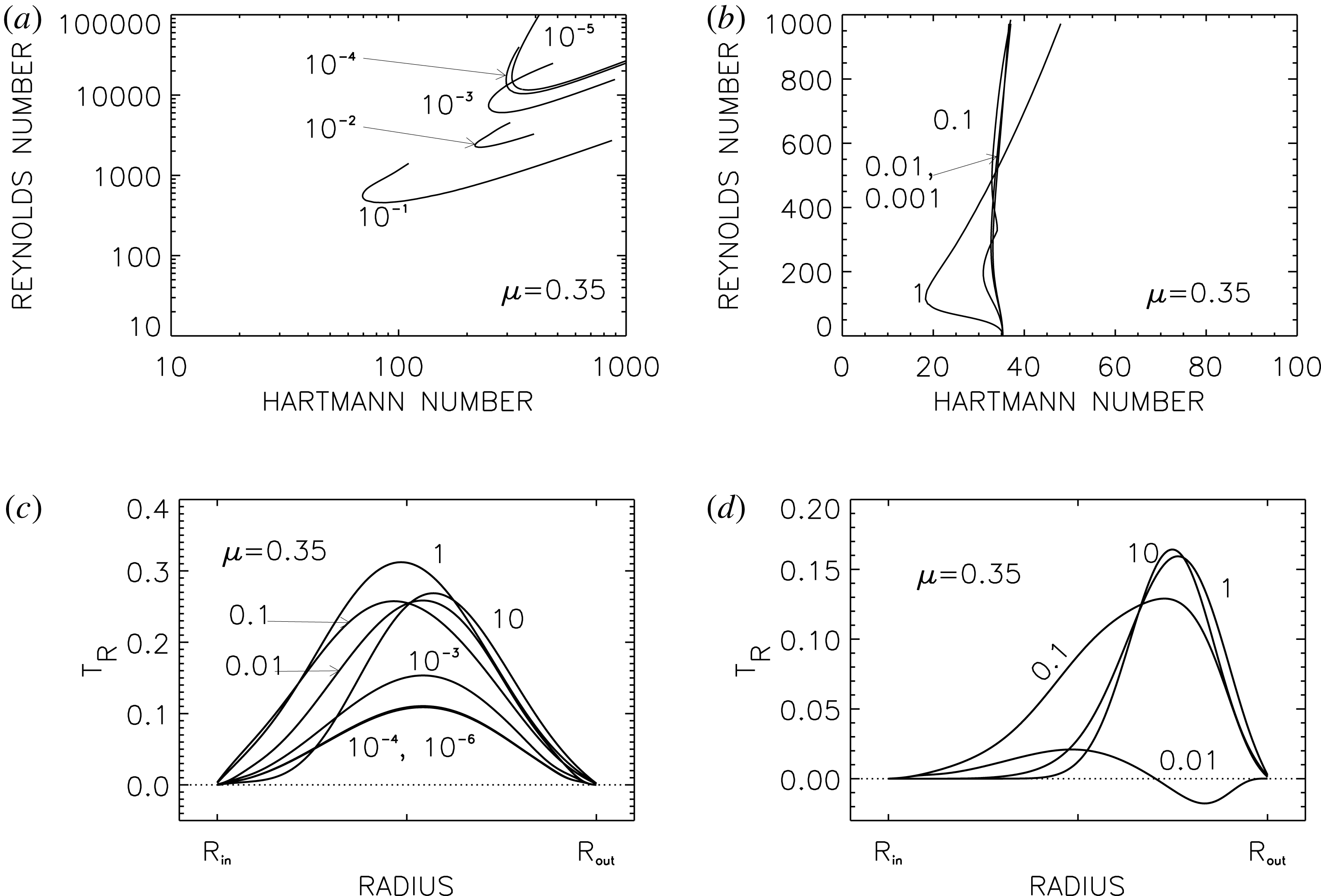
Quasi-Keplerian rotation. (a,b) Stability maps for
 $\unicode[STIX]{x1D707}_{B}=0.7$
(a, Chandrasekhar-type) and
 $\unicode[STIX]{x1D707}_{B}=2$
(Kepler pinch,
 $\text{Ha}_{0}=35.3$
, b). (c,d) Resulting angular momentum transport for the same flows. The curves are marked with their values of
 $\text{Pm}$
. The Hartmann numbers are
 $\text{Ha}=\text{Ha}_{\min }$
for
 $\unicode[STIX]{x1D707}_{B}=0.7$
and
 $\text{Ha}=50$
for
 $\unicode[STIX]{x1D707}_{B}=2$
.
 $r_{\text{in}}=0.5$
,
 $\unicode[STIX]{x1D707}=0.35$
,
 $m=\pm 1$
. Perfectly conducting cylinders.

The stability map for the field profiles fulfilling the Chandrasekhar condition combines typical properties of the maps of AMRI and of the Tayler instability. Figure 6(a) gives the lines of neutral stability for the field with
 $\unicode[STIX]{x1D707}_{B}=0.7$
. The curves for all
 $\text{Pm}$
possess crossing points
 $\text{Ha}_{0}$
with the horizontal axis (
 $\text{Re}=0$
, here not visible) but they also possess the absolute minimum Hartmann numbers
 $\text{Ha}_{\min }$
with
 $\text{Ha}_{\min }<\text{Ha}_{0}$
. The curves for very small
 $\text{Pm}$
coincide. For small magnetic Prandtl numbers the
 $\text{Ha}_{\min }$
(and also the associated Reynolds numbers) for the Chandrasekhar flow are rather small. Chandrasekhar-type fields are thus more unstable than fields which are current free between the cylinders (Kirillov & Stefani Reference Kirillov and Stefani2013). Even more unstable is the
 $z$
-pinch with
 $\unicode[STIX]{x1D707}_{B}=2$
combined with quasi-Keplerian rotation (‘Kepler pinch’) where the instability is already excited for very small Hartmann numbers
 $\text{Ha}_{0}=35.3$
(independent of the magnetic Prandtl number, see figure 6
b).
The first question is whether the quasi-Keplerian flow with
 $\unicode[STIX]{x1D707}_{B}=0.7$
also provides an anomalous angular momentum transport as the rigidly rotating
 $z$
-pinch which is also of the Chandrasekhar type. For many
 $\text{Pm}$
the angular momentum transport has thus been calculated at
 $\text{Ha}=\text{Ha}_{\min }$
(figure 6
c) and for the Kepler pinch with
 $\text{Ha}=50$
(figure 6
d). The results provide positive
 $T_{R}$
for all
 $\text{Pm}$
without any exception. An anomalous angular momentum transport does thus not exist for the two given examples with quasi-Keplerian rotation law.
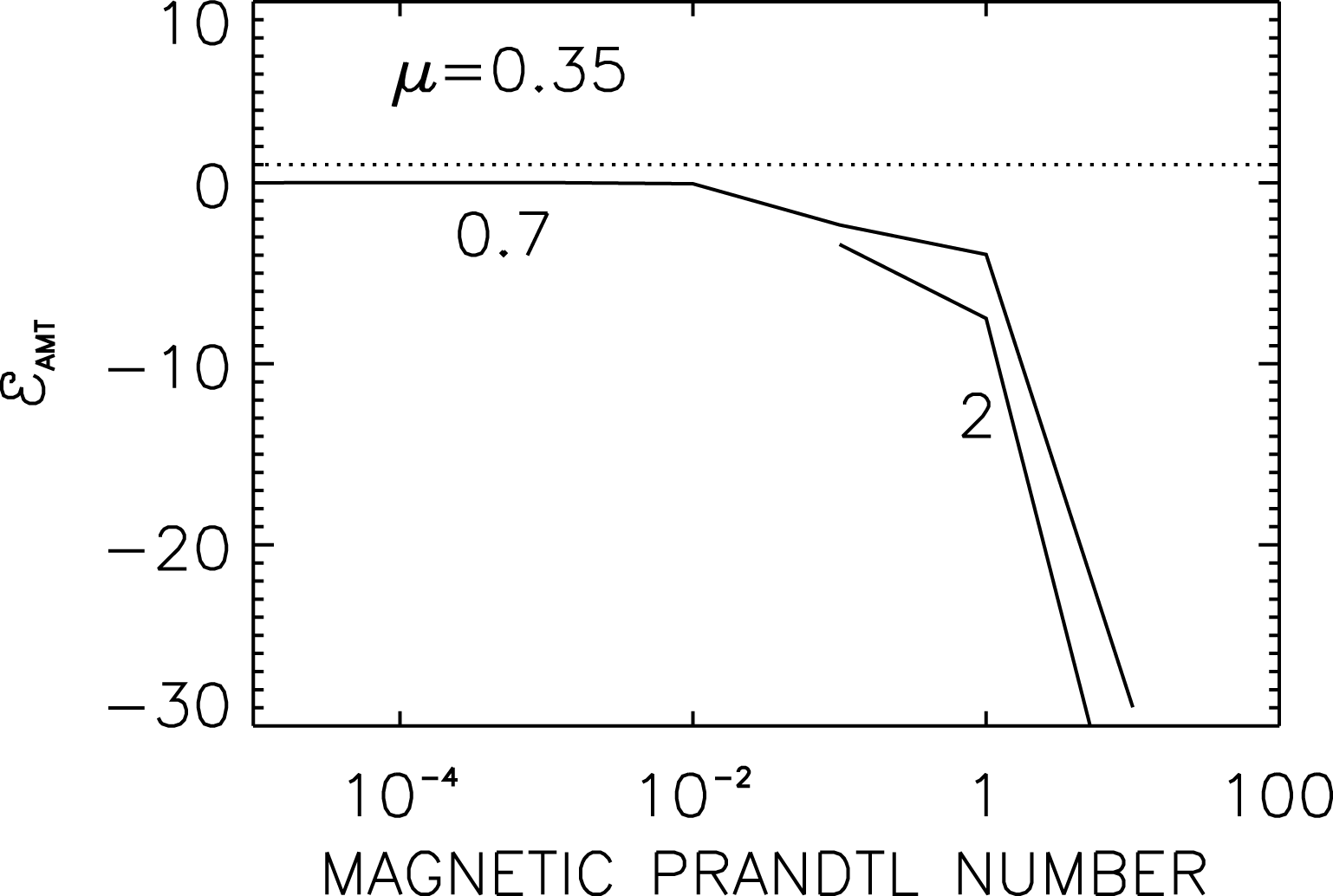
In order to demonstrate the basic influence of the magnetic Prandtl number on the contribution of the Maxwell stress to the angular momentum transport, figure 7 gives the stress ratio
 $\unicode[STIX]{x1D700}_{\text{AMT}}$
for the Chandrasekhar-type flow with quasi-Keplerian rotation and the Kepler pinch. Up to a magnetic Prandtl number of
 $10^{-2}$
the Maxwell stress is not important but for larger
 $\text{Pm}$
it is (because of
 $|\unicode[STIX]{x1D700}_{\text{AMT}}|\gg 1$
). Yet for these examples with growing magnetic Prandtl number also the magnetic Reynolds number grows. One always finds
 $\unicode[STIX]{x1D700}_{\text{AMT}}<0$
so that
 $\langle u_{R}u_{\unicode[STIX]{x1D719}}\rangle >0$
and
 $\langle b_{R}b_{\unicode[STIX]{x1D719}}\rangle <0$
for all magnetic Prandtl numbers. Both the Reynolds stress as well as the Maxwell stress are thus transporting angular momentum outwards. As expected for negative shear,
 $b_{R}$
and
 $b_{\unicode[STIX]{x1D719}}$
are anticorrelated. Mainly the Maxwell stress transports the angular momentum outward but this is only true for large magnetic Prandtl numbers.
Stress ratio (3.1) for the quasi-Keplerian flows in figure 6. The Hartmann numbers are
 $\text{Ha}=\text{Ha}_{\min }$
for the Chandrasekhar-type flows (
 $\unicode[STIX]{x1D707}_{B}=0.7$
) and
 $\text{Ha}=50$
for the Kepler pinch (
 $\unicode[STIX]{x1D707}_{B}=2$
). The horizontal dotted line symbolizes the ratio being unity,
 $\unicode[STIX]{x1D700}_{\text{AMT}}=1$
. Volume averages.
 $\unicode[STIX]{x1D707}=0.35$
,
 $m=\pm 1$
,
 $r_{\text{in}}=0.5$
. Insulating cylinders.

After the Boussinesq relation (1.4), a
 $z$
-pinch with negative shear generates positive
 $T_{R}$
for all
 $\text{Pm}$
. At least for
 $\text{Pm}=0.1$
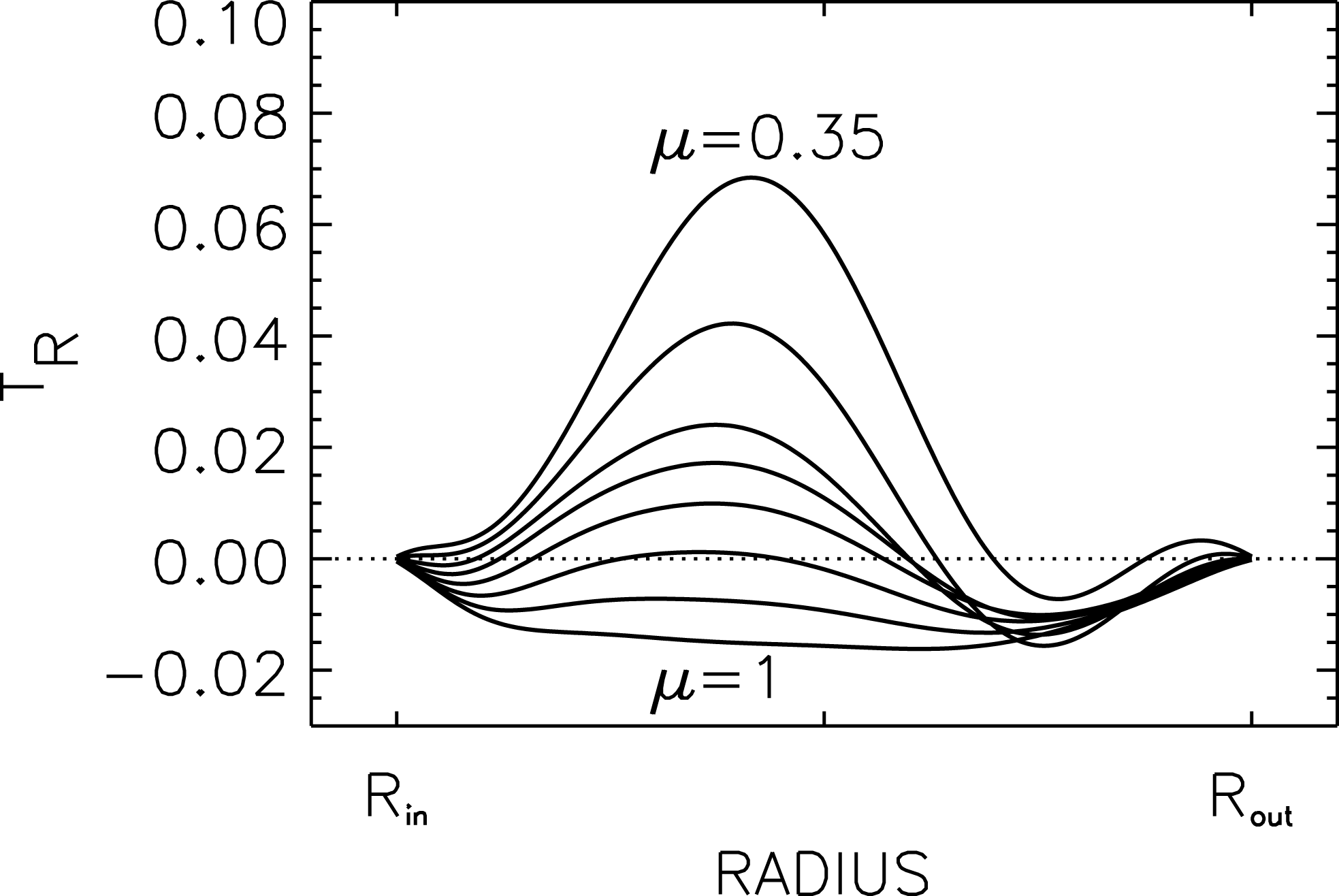
there must a transition exist between the negative values for rigid rotation and the positive values for, e.g. quasi-Keplerian rotation, as shown by figure 6. The questions arise as to whether this transition is continuous and for which rotation law the angular momentum flux vanishes. For the rotation laws with
 $1\geqslant \unicode[STIX]{x1D707}\geqslant 0.35$
the normalized values of
 $T_{R}$
within the cylindrical gap for
 $\text{Ha}=50$
are given in figure 8.
One finds
 $T_{R}$
vanishing for
 $\unicode[STIX]{x1D707}\simeq 0.75$
. If (1.4) is modified to
 $$\begin{eqnarray}T_{R}=\unicode[STIX]{x1D6EC}\unicode[STIX]{x1D6FA}-\unicode[STIX]{x1D708}_{\text{T}}R\frac{\text{d}\unicode[STIX]{x1D6FA}}{\text{d}R},\end{eqnarray}$$
then
 $\unicode[STIX]{x1D708}_{\text{T}}=\unicode[STIX]{x1D6EC}\,\text{d}\log R/\text{d}\log \unicode[STIX]{x1D6FA}$
for
 $\unicode[STIX]{x1D707}=0.75$
. In the sense of a heuristic estimate
 $\text{d}\log \unicode[STIX]{x1D6FA}/\text{d}\log R\simeq -2/3$
is used so that
 $$\begin{eqnarray}\unicode[STIX]{x1D708}_{\text{T}}\simeq 0.05\frac{E}{\unicode[STIX]{x1D6FA}}\end{eqnarray}$$
follows, with the total turbulence energy
 $E$
(see § 3). If
 $E$
can be replaced by
 $P/\unicode[STIX]{x1D70C}$
, with
 $P$
as the turbulence pressure, then (4.2) can be read as a confirmation of the viscosity approximation introduced by Shakura & Sunyaev (Reference Shakura and Sunyaev1973). Note that the numerical coefficient in (4.2) is basically smaller than unity. Although with a linear theory the function
 $E=E(\unicode[STIX]{x1D6FA})$
cannot be determined so the numerical calculation of the eddy viscosity must remain open. If it is allowed to work with magnetic-equilibrated ‘turbulence’, i.e.
 $E=u_{\text{rms}}^{2}=B_{\unicode[STIX]{x1D719}}^{2}/\unicode[STIX]{x1D707}_{0}\unicode[STIX]{x1D70C}$
then
 $$\begin{eqnarray}\frac{\unicode[STIX]{x1D708}_{\text{T}}}{\unicode[STIX]{x1D708}}\simeq 0.05\frac{\text{Ha}^{2}}{\text{Rm}}=\frac{0.05}{\text{Pm}~\text{Mm}}~\text{S},\end{eqnarray}$$
with
 $\text{S}$
the Lundquist number
 $\text{S}=\sqrt{\text{Pm}}\text{Ha}$
. As
 $\text{Mm}\simeq 2$
for neutral instability of rigidly rotating containers with
 $\text{Pm}=0.1$
, the estimation (1.4) is in excellent agreement with the result
 $\unicode[STIX]{x1D708}_{\text{T}}/\unicode[STIX]{x1D702}\simeq 0.01~\text{S}$
of complex nonlinear simulations (Rüdiger et al.
Reference Rüdiger, Gellert, Hollerbach, Schultz and Stefani2018).
Normalized angular momentum transport for non-uniformly rotating
 $z$
-pinches with
 $\unicode[STIX]{x1D707}=1$
to
 $\unicode[STIX]{x1D707}=0.35$
(marked).
 $\unicode[STIX]{x1D707}_{B}=2$
,
 $\text{Ha}=50$
,
 $m=\pm 1$
,
 $\text{Pm}=0.1$
,
 $r_{\text{in}}=0.5$
. Perfectly conducting cylinders.

5 Conclusions
We have shown that for the magnetic instability of azimuthal fields the angular momentum transport can often be modelled by the diffusion approximation (1.4), but not always. Exceptions exist for rigidly rotating tubes with radially increasing magnetic toroidal magnetic fields where the electric current flows parallel to the rotation axis. The resulting non-vanishing radial angular momentum flux excludes solid-body rotation as a solution of the MHD equation system of rotating pinches.
For reasons of the consistency our models are mostly located along the lines of neutral stability for given functions
 $\unicode[STIX]{x1D6FA}(R)$
and
 $B_{\unicode[STIX]{x1D719}}(R)$
where the growth rates vanish. In one case we also proceeded along a vertical slice in the (
 $\text{Ha}/\text{Re}$
) plane with a fixed Hartmann number (
 $\text{Ha}=50$
) for Reynolds numbers smaller than
 $\text{Re}_{\max }$
where the growth rates are positive. The results also demonstrate the existence of non-vanishing angular momentum fluxes even exceeding the values of
 $T_{R}$
obtained for
 $\text{Re}_{\max }$
.
Among the fields probed for angular momentum transport are also those of the Chandrasekhar-type where the magnetic field
 $B_{\unicode[STIX]{x1D719}}$
has the same radial profile as the linear velocity
 $U_{\unicode[STIX]{x1D719}}$
of the rotation. The instability curves of such Chandrasekhar-type systems coincide for small
 $\text{Pm}$
in the (
 $\text{Ha}/\text{Re}$
) plane. Prominent examples of this unique class of MHD flows are the rigidly rotating
 $z$
-pinch (flow and field are linearly running with
 $R$
) and also the quasi-Keplerian rotation combined with a magnetic field with
 $B_{\unicode[STIX]{x1D719}}\propto 1/\sqrt{R}$
. For both constellations one finds finite values of the angular momentum transport. It is positive (outward flow of angular momentum) for the quasi-Keplerian rotation for all
 $\text{Pm}$
and for the uniformly rotating pinch for large magnetic Mach number. For sufficiently slow rigid rotation and not too large
 $\text{Pm}$
it is negative, i.e. the angular momentum flows inward.
For small magnetic Prandtl numbers the contribution of the Maxwell stress to the angular momentum flow is always small but the Reynolds stress
 $\langle u_{R}u_{\unicode[STIX]{x1D719}}\rangle$
is negative. For the larger
 $\text{Pm}$
the transport is always outward due to the dominating negative Maxwell stress,
 $\langle b_{R}b_{\unicode[STIX]{x1D719}}\rangle <0$
, as expected for rotation with negative shear.
Stability map (a) and radial angular momentum transport (b) for uniform rotation and quasi-uniform magnetic field for various magnetic Prandtl numbers (marked).
 $\text{Ha}_{0}=150$
for
 $\text{Re}=0$
.
 $\unicode[STIX]{x1D707}=\unicode[STIX]{x1D707}_{B}=1$
,
 $m=\pm 1$
,
 $r_{\text{in}}=0.5$
. Perfectly conducting cylinders.

We have probed the surprising finding for rigid rotation also with the quasi-uniform magnetic field profile (
 $\unicode[STIX]{x1D707}_{B}=\unicode[STIX]{x1D707}=1$
). Flow and field of this model (which is not of the Chandrasekhar-type) are only unstable for
 $\text{Mm}<0.5$
. Again, a finite angular momentum transport exists which is directed inward for
 $\text{Pm}=0.1$
while it is directed outward for smaller and larger
 $\text{Pm}$
(figure 9). Obviously, the radial profile of the magnetic field does not play the decisive role for the existence of the
 $\unicode[STIX]{x1D6EC}$
effect by magnetic instabilities.
The phenomenon that a rigidly rotating magnetized Taylor–Couette flow of a given magnetic Mach number transports angular momentum cannot be described by the diffusion approximation (1.4). It forms a magnetic counterpart to the hydrodynamical
 $\unicode[STIX]{x1D6EC}$
effect in rotating anisotropic turbulence. It also means that solid-body rotation can neither be maintained in rotating convection zones nor in rotating tanks with a conducting fluid and a supercritical electric current flowing in the
 $z$
-direction.
It also makes sense to study the transition of the angular momentum flux from uniform rotation (inward transport) to quasi-Keplerian rotation (outward transport). Figure 8 demonstrates how the anomalous angular momentum transport disappears if the rotation law becomes more and more non-uniform. At a certain shear value the angular momentum flux vanishes. For the
 $z$
-pinch with
 $\text{Pm}=0.1$
the transport vanishes for
 $\unicode[STIX]{x1D707}\simeq 0.75$
where
 $\unicode[STIX]{x1D6EC}$
effect and viscous transport compensate each other. This result can be used for an approximated evaluation of the eddy viscosity. The related expression formally explains the formulation of Shakura & Sunyaev (Reference Shakura and Sunyaev1973) and numerical values hardly differ from the results of nonlinear simulations presented earlier.