Nomenclature

ACU

antenna control unit

Az

azimuth

BER

bit error rate

CKF

cubature Kalman filter

dBi

decibels relative to an isotropic antenna

dBm

decibels relative to 1 milliwatt

EKF

extended Kalman filter

El

elevation

FFT

fast Fourier transform

IF

intermediate frequency

GS

ground station

HRTX

high-rate transmitter

LCMV

linearly constrained minimum variance

LEO

low earth orbit

LHCP

left-hand circular polarisation

LNA

low-noise amplifier

MS

multispectral

MSE

mean squared error

PAN

panchromatic

PID

proportional integral derivative

PSO

particle swarm optimisation

RF

radio frequency

RHCP

right-hand circular polarisation

RMSE

root mean squared error

RPY

roll pitch yaw

STK

systems tool kit

TC

telecommand

TCC

tracking coupler-combiners

TLE

two-line elements

TSR

tracking signal receiver

TM

telemetry

UAVs

unmanned aerial vehicles

2.0 Oran gs tracking system architecture

The antenna tracking system deployed at the Oran GS is of monopulse type. It is equipped with a 7.3-meter parabolic reflector [Reference Bekkar Djelloul Saiah20] and is based on three functional blocks: a tracking coupler-combiner (TCC), a tracking signal receiver (TSR) and an antenna control unit (ACU), as depicted in Fig. 1.

Figure 1.

Architecture of the GS antenna tracking system (Oran site).

The TCC block receives RF signals from multiple antenna feed elements that capture incoming satellite transmissions. Using a network of hybrid phase shifters configured with phase delays of 0 deg, 90 deg, 180 deg, and 270 deg, the system generates three primary output signals: the sum channel Q(R), corresponding to the main beam or boresight direction, and the difference channels Δx and Δy, which indicate angular deviations along the Az (X-axis) and El (Y-axis), respectively. These signals are mathematically defined as follows [Reference Latifzade, Arvan and Mohseni Armaki25]:

(1) \begin{align}Q(R) = \;{E_1} + {E_2} + {E_3} + {E_4}\;,\end{align}

(2) \begin{align}\Delta x{\rm{\;}} = {\rm{\;}}\left( {{E_1} + {E_2}} \right) - {\rm{\;}}\left( {{E_3} + {E_4}} \right),\end{align}

(3) \begin{align}\Delta y{\rm{\;}} = {\rm{\;}}\left( {{E_1} + {E_4}} \right) - {\rm{\;}}\left( {{E_2} + {E_3}} \right){\rm{\;}},\end{align}

where ${E_1}$ , ${E_2}$ , ${E_3}$ and ${E_4}$ are the amplitude signals obtained from first, second, third and fourth horns, respectively.

The signals generated through the TCC, as defined in Equations (Reference Hughes and Moy1), (2) and (Reference Edwards3), are amplified using low noise amplifiers (LNA) to ensure optimal signal level and then transmitted to the TSR. Based on sigmoid model (refer to Assumption1), the Q(R) signal is extracted and normalised according to the reference signal ${S_{level}}$ , provided by the splitter. The choice of the sigmoid function is motivated by its ability to represent nonlinear behaviours with saturation, which are typical in tracking errors and dynamic control responses.

Assumption 1. A nonlinear transition function is used to model the behaviour of Q(R) as a function of the signal ${S_{level}}$ , which directly influences the tracking amplitude. We assume that the values are normalised in the interval $\left[ {\varepsilon ,1} \right]$ [Reference Kyurkchiev and Markov26]:

(4) \begin{align}Q(R) = \left\{\begin{array}{c@{\quad}c}1& if\,\, S_{level}\, \ll\, S_0\\{1 - \epsilon \over 1 + e^\alpha ( S_{level} - S_0)} + \epsilon &if\;\;S_{level} \,\approx\, S_0\\{ \epsilon} & if\;\;S_{level} \,\gg\, S_0 \end{array}\right.\end{align}

where ${S_0}$ is the threshold at which $Q(R)$ starts to decay and $\alpha $ is an adjustable parameter for the decay rate, ∈ is the desired minimum value $\left( {\epsilon \to 0} \right)$ .

This process allows an accurate estimation of the angular deviations ${e_{\theta x}}$ and ${e_{\theta y}}$ of the antenna with respect to the direction of the target satellite, as defined by the following Equations [Reference Sherman and Barton27]:

(5) \begin{align}{e_{\theta x}} = \sigma .{{\Delta x\;} \over {Q(R)}},\end{align}

(6) \begin{align}{e_{\theta y}} = \sigma .{{\Delta y\;} \over {Q(R)}},\end{align}

where $\sigma $ is the sensitivity of the monopulse system to small angular changes.

Assumption 2. The angular deviations ${e_{\theta x}}$ and ${e_{\theta y}}$ are inversely proportional to the normalised quality of the received signal, $N\left[ {Q(R)} \right]$ . As the received signal weakens (i.e. $N\left[ {Q(R)} \right]$ approaches 1, the angular estimation errors in both the X and Y planes increase significantly. Conversely, when the signal is strong (i.e. $N\left[ {Q(R)} \right] \to 0$ ), the system achieves higher angular localisation accuracy in both directions [Reference Van Trees28].

These angles are then transmitted to a proportional integral derivative (PID) controller [Reference Uthman and Sudin29], which continuously adjusts the antenna’s orientation based on the angular error. The PID controller equation is given by:

(7) \begin{align}\left\{ {\begin{array}{*{20}{c}}{{u_{\theta x}}(t) = \;{k_p}{e_{\theta x}}(t) + {k_i}\displaystyle\mathop \int \nolimits_0^t {e_{\theta x}}\left( \tau \right)d\tau + {k_d}\frac{{d{e_{\theta x}}(t)}}{{dt}}\;}\\[12pt]{{u_{\theta y}}(t) = \;{k_p}{e_{\theta y}}(t) + {k_i}\displaystyle\mathop \int \nolimits_0^t {e_{\theta y}}\left( \tau \right)d\tau + {k_d}\frac{{d{e_{\theta y}}(t)}}{{dt}}\;}\end{array}} \right.\end{align}

where the control signal outputs, ${u_{\theta x}}(t)$ and ${u_{\theta y}}(t)$ , correspond to the directions of the upper motor along the $\;x$ -axis and the lower motor along the $y$ -axis. The terms ${k_p}$ , ${k_i}$ and ${k_d}$ represent the proportional, integral and derivative gains.

3.0 Particle swarm optimisation

The PSO algorithm, a metaheuristic method inspired by swarm behaviour, is used here to adjust and improve the parameters of the auto-tracking system. Each particle has a randomly initialised velocity and position. It maintains two key positions: its best local position $\overrightarrow {{p_i}} = \left( {{p_{i1}},{p_{i2}}, \ldots ,{p_{iD}}} \right)$ and the best global position $\vec g = \left( {{g_1},{g_2}, \ldots ,{g_D}} \right)$ , corresponding respectively to the best solution found individually and collectively by all the particles. The position $\overrightarrow {{p_i}} $ represents the particle’s local memory and guides its movement based on its individual experience. In contrast, $\vec g$ reflects the collective intelligence of the swarm and constitutes the true solution delivered by the algorithm. This approach ensures that the final solution does not depend on a single particle, but results from a collective compromise, thereby enhancing the robustness and quality of the optimisation. In this work, $\vec g$ is considered the optimal solution, namely the one that minimises the fitting function defined hereinafter.

The position vector ${\vec x_{ij}} = \left( {{x_{i1}},{x_{i2}}, \ldots ,{x_{iD}}} \right)$ and the velocity vector ${\vec v_{ij}} = \left( {{v_{i1}},{v_{i2}}, \ldots ,{v_{iD}}} \right){\rm{\;}}$ are updated at each iteration according to the following equations [Reference Kennedy and Eberhart30, Reference Boualem31]:

(8) \begin{align}{x_{ij}}( t ) = {x_{ij}}( {t - 1} ) + {v_{ij}}( t )\,;\,( {j=1,2,3 \ldots D} )\end{align}

(9) \begin{align}{v_{ij}}(t) = {\rm{\;}}\omega {v_{ij}}( {t - 1} ) + {c_1}{r_1}( {{p_{ij}}} ((t - 1) - {x_{ij}}( {t - 1} )) + {c_2}{r_2}({g_j}\left( {( {t - 1} ) - {x_{ij}}( {t - 1} )} \right)\end{align}

where ω is generally a constant called coefficient of inertia, ${r_1}$ and ${r_2}$ are randomly selected in the interval $\left[ {0,1} \right]$ , ${c_1}$ and ${c_2}$ are acceleration coefficients that influence the motion of a particle.

The following equation delineates the fitting function employed in the optimisation of Q(R) parameters, presented as:

(10) \begin{align}minf\!\!\left( {{S_0},\alpha } \right) = MSE + {\rm{\;}}{\lambda _1}\left| {{S_0} - 71} \right| + {\lambda _2}\left| {\alpha - 1} \right|\end{align}

The mean square error ( ${\rm{MSE}}$ ) between the model and the actual data is given by:

(11) \begin{align}MSE = {1 \over N}\mathop \sum \limits_{i = 1}^N {\left( {Q{{\left( R \right)}_i} - \hat Q{{\left( R \right)}_i}\;} \right)^2}\end{align}

where ${\hat Q{{\left( R \right)}_i}\;}$ is the measured signal value, $N$ is the total number of points, and $\left\{ {{\lambda _1},{\rm{\;}}{\lambda _2}} \right\}\; \in {\mathbb R}$ denotes the respective weights for the performance indices.

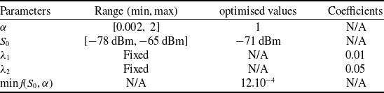
Table 1 shows the results generated by the learning process using the PSO algorithm, as well as the corresponding fitting function (see Fig. 2).

Table 1.

Optimisation of auto-tracking system parameters using PSO

Figure 2.

Parametric sensitivity analysis of the fitting function over ${{\rm{S}}_0}{\rm{\;}}$ and ${\rm{\alpha }}.$

The sequential process of the optimisation algorithm unfolds through the following steps:

Step 1: Initialisation

• • Define the PSO optimisation parameters:

  1. 1. Define the search bounds for ${S_0}$ and $\alpha $ .

  2. 2. Determine the precision threshold ∈.

  3. 3. Specify the number of particles and the maximum number of iterations $Max\_iter$ .

Step 2: Define the fitting function

• • Compute the fitting function based on Equation (Reference Benzeniar10), which evaluates the quality of a given solution.

Step 3: Perform the PSO optimisation (if Iter > 1)

• • For each iteration, calculate the fitting function for each particle

  1. 1. Update the particle positions using velocity Equations (Reference Varotsos and Cracknell8) and (Reference Darfilal and Gibbon9).

  2. 2. Find the best solution among all particles.

  3. 3. Display the optimal values of ${S_0}$ and $\alpha $ .

Step 4: Check Termination Criteria

• • If the minimum value $minf\!\!\left( {{S_0},\alpha } \right)$ falls below a predefined small tolerance value $\epsilon$ , or the maximum number of iterations $Max\_iter$ is achieved:

  • − Report the best solution, which is the PSO, and conclude the algorithm.

• • If the termination conditions are not satisfied:

  • − Return to Step 3 to execute the subsequent iteration and remain in the optimisation process.

4.0 Experimental setup

To evaluate the effectiveness of the design implemented for the X-band GS in Oran, a series of experimental tests were conducted. The system relies primarily on the use of ephemeris transmitted by the control centre based on two line elements (TLE), allowing the satellite trajectory to be anticipated. The antenna dynamically adjusts its angular positions (upper X and lower Y, corresponding to ${\theta _{x,{\rm{\;}}target}}$ and ${\theta _{y,{\rm{\;}}target}}$ ), based on the signal strength received from the satellite. This is achieved through a monopulse tracking mode, ensuring optimal antenna pointing throughout the entire visibility period. To support this operation, the antenna system offers axis travel spans of ±90 deg, with a maximum angular velocity of 4 deg/s and an angular acceleration of 10 deg/s. The pointing limits extend to about 91 deg (i.e. 1° below the horizon), while the X/Y drive motors, based on DC brushless servo technology, guarantee precise and reliable tracking performance.

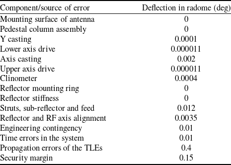
Based on these operational capabilities, the resulting pointing errors, which are approximately 0.6 deg, have been evaluated and are summarised in Table 2, including a security margin to account for uncertainties, particularly at high elevation angles approaching 90 deg.

Figure 3 presents the specification of the antenna radiation pattern in X-band: maximum gain of 55.49 dBi at the nominal pointing direction (0°) and a beamwidth of 0.6° (±0.3°).

Figure 3.

X-band antenna radiation pattern specification.

The GS is configured with a TM frequency of $2266.5{\rm{\;MHz}}$ and a TC frequency of $2087.1{\rm{\;MHz}}$ in the S-band [Reference Bensikaddour, Nasri, Bouchiba, Baba Hamed and Bekkar Djelloul Saiah32]. In the X band, the telemetry frequency is $8070{\rm{\;}}MHz$ , which corresponds to an IF of 720 ${\rm{MHz}}$ . The transmission rate is set at $80{\rm{\;Mbps}}$ , which corresponds to the high-rate transmitter (HRTX) device.

The ALSAT-2B satellite was selected for several X-band image download sessions, scheduled during its flybys of the station. It is positioned in a near-circular sun-synchronous orbit, with an inclination of $98.0044$ ${\rm{deg}}$ and an altitude of $665.27\;{\rm{km}}$ . ALSAT-2B features agile pointing capabilities, allowing real-time attitude adjustments to acquire off-nadir imagery at multiple angles.

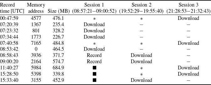
As part of the experiment presented in this article, three onboard image download sessions were conducted, resulting in the acquisition of 11 PAN and MS images on March 24, 2025, for a cumulative volume of 4,640.58 MB. Session 1 included both image capture and image downloading, while sessions 2 and 3 were exclusively dedicated to downloading the acquired images. Table 3 summarises the recording times, the onboard memory addresses scheduled for the download and the size of each image file.

Figure 4 shows the evolution of the roll, pitch and yaw angles of the ALSAT-2B satellite over a 24-hour period, extending from March 23, 2025, at 21:15:22, to March 24, 2025, at 21:37:04. The image acquisition times are represented by identifiable contours on the curve.

Table 2.

Summary and accumulation of pointing errors

Table 3.

Scheduled ALSAT-2B image acquisitions and related operations

${\blacksquare}$ : The image has not yet been taken

*: The image is stored in the satellite’s mass memory

$ - $ : The image has already been downloaded and removed from mass memory

Figure 4.

Attitude dynamics of ALSAT-2B over time.

However, for the detailed analysis conducted in this study, only sessions 1 and 3, corresponding to two distinct scenarios, were retained. Session 2 was not taken into account due to its strong operational similarity with session 3.

4.1 Scenario 1

The 3D representation of the pass for this scenario (satellite antenna not aligned with GS) was extracted from the control centre’s tracking software, where ALSAT-2B follows a descending orbit (see Fig. 5).

Figure 5.

3D representation of the pass for scenario 1.

The pass began with an acquisition of signal (AOS) time of 08:57:21, corresponding to the activation of the satellite’s HRTX, and ended with a loss of signal (LOS) time of 09:00:52, marking the deactivation of the HRTX. During this period, the satellite simultaneously captured images (recorded 08:53:42 and 08:58:43) and transmitted the images that were already on board. This phase triggered notable variations in roll, pitch and yaw, with attitude variations ranging from approximately $ - 20{\rm{\;}}deg$ to $+20{\rm{\;}}deg$ , clearly visible within the HRTX activation window (see Fig. 6).

Figure 6.

HRTX activations based on satellite behaviour for scenario 1.

Figure 7 shows that the signal received by the station remains stable around $ - 75{\rm{\;dBm}}$ between 08:56:00 and 08:57:10, indicating that the auto-track system was inactive during this period, according to Fig. 8 $({\rm{N}}\left[ {Q(R)} \right]{\rm{\;}} \to {\rm{\;}}1{\rm{\;}}and{\rm{\;}}{S_{level}}{\rm{\;}} \lt \;{S_0} = {\rm{\;}} - 71{\rm{\;}}dBm)$ . Between 08:57:42 and 09:00:42, a significant increase in signal strength around $+20{\rm{\;dBm}}$ is observed, with values ranging from −57.22 dBm to −54.83 dBm, indicating activation of the auto-track system. However, during the interval from 08:58:02 to 08:58:23, a ${\rm{N}}\left[ {Q(R)} \right]{\rm{\;}}$ error in the order of 10^-3 caused a moderate drop in signal strength, estimated at approximately −5 dBm. This suggests that the system was readjusting to improve its alignment with the satellite, consistent with the scheduled image acquisition maneuvers. Subsequently, from 08:59:00 to 09:00:00, the system remained stable, with ${\rm{N}}\left[ {Q(R)} \right]$ approaching zero.

Figure 7.

X-band signal level during HRTX activations (scenario 1).

Figure 8.

Normalised Q(R) values versus auto-track usage (scenario 1).

The angular deviations of the antenna from the satellite direction are shown in Fig. 9. Activating the auto-tracking function enabled the motor encoders to accurately align with the target, reaching maximum correction values of $0.14{\rm{\;deg}}$ on the X-axis and $0.036{\rm{\;deg}}$ on the Y-axis. 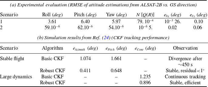The variation in angular errors, given by equation $\Delta {e_{\theta i}}(t) = {e_{\theta i}}(t) - {e_{\theta i}}\left( {t - 1} \right),$ with $i \in \{ {x,y} \}$ , are shown in Fig. 10. They reflect the successive adjustments of the pointing system, illustrating the subtle movements of the antenna to maintain optimal orientation (see Table 4).

Table 4.

Comparative results under different scenarios

Figure 9.

Angular deviation values during auto-track activation (scenario 1).

Figure 10.

Variation in angular errors during auto-tracking (scenario 1).

4.2 Scenario 2

Depicted in Fig. 11 (satellite antenna aligned with GS). During this pass, ALSAT-2B is in an ascending orbit.

Figure 11.

3D representation of the pass for scenario 2.

The pass for this scenario enabled the satellite’s HRTX to be activated for image download, without any image capture operation. A variation of ±10^-5 degrees was recorded on the roll, pitch and yaw axes. This pass extended from AOS: 21:28:53 to LOS: 21:32:43 (see Fig. 12).

Figure 12.

HRTX activations based on satellite behaviour for scenario 2.

As shown in Fig. 13, the signal level increased from −60.53 dBm to −54.55 dBm between 21:28:43 and 21:33:02, respectively, reflecting the accurate activation of the auto-track system. The observed stability can be attributed to the absence of image acquisition during this interval, in contrast to scenario 1. Throughout this period, the system remained stable, with ${\rm{N}}\left[ {Q(R)} \right]$ values close to zero $\left( {{{10}^{ - 6}}} \right)$ as illustrated in Fig. 14.

Figure 13.

X-band signal level during HRTX activations (scenario 2).

Figure 14.

Normalised Q(R) values versus auto-track usage (scenario 2).

On the other hand, for scenario 2, we observe that the angular deviations of the antenna with respect to the direction of the satellite, as illustrated in Fig. 15, are precise and stable. This confirms that the pointing system has made successive adjustments, as shown in Fig. 16. The variation of the angular errors on the X axis remains less than $0.005{\rm{\;deg}}$ , while that on the Y axis does not exceed $ - 0.017{\rm{\;deg}}$ (see Table 4).

Figure 15.

Angular deviation values during auto-track activation (scenario 2).

Figure 16.

Angular error evolution during auto-tracking (scenario 2).

Table 4 shows the root mean square error (RMSE) values of ALSAT-2B attitude estimates relative to the GS direction for both download sessions, with the work reported in Ref. (Reference Xuan, Ruo-xin and Yi-feng24) included as a reference for comparison.

The comparison shows that the proposed method achieves much smaller angular deviations than both basic and robust CKF. While the basic CKF may exceed one degree and the robust CKF reduces errors to a few tenths of a degree, our approach maintains values below 0.1 deg even under experimental conditions, confirming superior accuracy, stability, and robustness.