I. INTRODUCTION
Polymers are noted for their pronounced time- and temperature-dependent mechanical properties, including yield. Rate and temperature effects in the yield stress are a consequence of the mechanisms for plastic flow, which involve thermally activated chain rearrangements and side group motions.Reference Boyer1, Reference Argon2 Although rate and temperature effects are important in their own right, they can also be used as “fingerprints” to help gain insight into deformation mechanisms and polymer structure (e.g., Refs. Reference Mayr, Cook and Edward3–Reference Kazmierczak, Galeski and Argon7). Approaches involving uniaxial compression, tension, or shear experiments are well established for bulk specimens to assess the temperature and rate dependence of yielding.
It is desired to extend studies of rate and temperature dependence of yielding to microscopic polymer systems including thin filmsReference Strojny, Xia, Tsou and Gerberich8, Reference Warren and Wyrobek9 and components in biological materials.Reference Ebenstein and Pruitt10, Reference Jakes, Frihart, Stone, Katti, Hellmich, Wegst and Narayan11 One way to do this is to rely on indentation creep, which has been used for more than 50 years in polymers.Reference Rostoker and Galante12, Reference Takahashi, Shen, Taylor and Tobolsky13 Indentation creep involves pushing a hard (typically diamond), pyramid- or sphere-shaped indenter into the specimen until a predetermined load is reached, then holding the load constant. The constant load portion of the experiment is analyzed. At constant load, the indenter continues to penetrate so that area of contact grows as a function of time. The pressure, or hardness, beneath the indenter and the rate of penetration both decrease with time giving rise to a spectrum of hardness versus strain rate. A similar experiment is impression creep in which the end of a right circular cylinder is used.Reference Chu and Li14 Because the area stays constant during creep, the experiment is less ambiguous to interpret, but the load must be varied to achieve different levels of stress.
With advances in instrumentation over the past 20 years (nanoindentation), indentation creep can now readily be applied to probe rate effects in submicron volumes of material. However, there remains a lack of consensus on how best to perform and interpret indentation creep experiments in polymers. A common practice is to fit creep data to specific mathematical equations or spring and dashpot models, and then to back out material parameters from the fits.Reference Chen, Bell, Hanshan, Smith and Beake15–Reference Li and Ngan18 Some analyses assume the deformations are viscoelastic,Reference Constantinides, Tweedie, Holbrook, Barragan, Smith and Van Vliet19–Reference Vanlandingham, Chang, Drzal, White and Chang25 whereas others account for both viscoelastic and viscoplastic deformations.Reference Beake26, Reference Zhang, Zhang, Zeng and Shen27 The distinction between viscoelasticity and viscoplasticity in polymers can be gradual, and the problem of separating the two is compounded when a Berkovich indenter is used, whose characteristic strain of about 7–8% is comparable to the strain at the onset of yield. Yet, Berkovich indenters are readily available, convenient to use, and because they are self-similar they can be used to probe properties across a wide range of length scales while maintaining the average strain beneath the indenter constant.
Our goal is to develop methods for obtaining robust and unambiguous measurements of viscoelasticity and viscoplasticity with Berkovich indenters without having to constrain the analyses by relying on constitutive models or having to make unverified assumptions of material behavior. In the accompanying article,Reference Jakes, Lakes and Stone28 we evaluated viscoelastic moduli from unloading slopes of nanoindentation traces in glassy polymers. Here we assess viscoplasticity in the same materials by using the constant load creep portion of the nanoindentation trace. It turns out that the experiments and analysis require minimal assumptions about material behavior, and the connection between rate-dependent hardness and rate-dependent yield stress becomes immediately apparent when the two are compared across a wide range of strain rate.
For each instant in time during indentation creep, instantaneous Meyer hardness is defined as the average pressure beneath the indenter,

where P is the applied load and A is the instantaneous projected contact area. The material strain rates beneath the indenter fall across a distribution. The median of this distribution scales in proportion to indentation strain rate, which we define asReference Elmustafa, Kose and Stone29
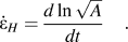
In the present work, we measure the H– properties of the glassy polymers poly(methylmethacrylate) (PMMA), polystyrene (PS), and polycarbonate (PC) using broadband nanoindentation creep (BNC)Reference Puthoff, Jakes, Cao and Stone30 to access as wide a range of strain rate as possible (10−4 to 10 s−1). To better understand the physical significance of H, we present two methods for converting H–
 to compression yield stress–strain rate (σ–
 ). With both methods, the σ–
 derived from BNC agrees well with literature data. This means the same viscoplastic data can be obtained from indentation creep and uniaxial experiments. To make sure we are properly analyzing creep data from the polymers, we also perform BNC experiments on molybdenum (Mo), which serves as a control because its properties have been measured before, although not over such a wide range of strain rate,Reference Stone and Yoder31, Reference Yoder, Elmustafa, Lin, Hoffman and Stone32 and because its flow stress is less sensitive to hydrostatic pressure than those of the polymers.
II. EXPERIMENTAL WORK
The accompanying articleReference Jakes, Lakes and Stone28 provides complete details of the experimental work. Except where noted, all experimental procedures are the same.
A. Specimens
The same PMMA, PC, and PS glassy polymers prepared in the accompanying article are also used in this work. In addition, bulk Mo is studied. The Mo specimen was the same one studied previously by Stone and Yoder.Reference Stone and Yoder31 The surface of this specimen was freshly prepared by metallographic grinding and polishing down to 0.05-μm alumina.
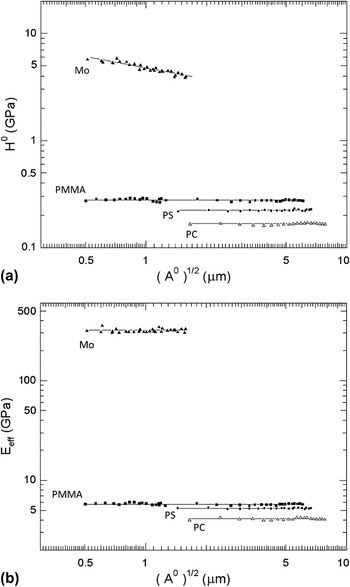
Before performing BNC experiments, we determined how the hardness and modulus depend on load in these materials. The motivation was to test for any depth dependence in material properties, which if present needs to be accounted for in the analysis of indentation creep.Reference Stone and Yoder31 The results shown in Fig. 1 are based on areas measured using atomic force microscope (AFM) images. Mo alone shows an indentation size effect in hardness over the range of loads tested. None of the materials tested exhibit a size effect in modulus. A method for checking the area measurements (and thereby verifying the presence or absence of indentation size effect in properties) is to determine machine compliance using two different methods: Doerner–Nix,Reference Doerner and Nix33 which requires knowledge of indent areas, and Stone–Yoder–Sproul correlation,Reference Stone, Jakes, Puthoff and Elmustafa34–Reference Jakes, Frihart, Beecher, Moon and Stone36 which does not. The indentation size effect is well known in large-grained metals.Reference Ma and Clarke37, Reference Nix and Gao38 There is less consensus on the behavior of glassy polymers at shallow depths. Some researchers have reported an indentation size effect for depths less than 100 nm (e.g., Refs. Reference Tweedie, Constantinides, Lehman, Brill, Blackman and Van Vliet39 and Reference Amitay-Sadovsky, Ward, Somorjai and Komvopoulos40), but this depth is shallower than any of our experiments except for the shallowest indent in PMMA.
Dependence of (a) Meyer hardness and (b) modulus on indent size. H 0 is the hardness immediately before unloading. Modulus (E eff) was measured using methods described in the accompanying article.Reference Jakes, Lakes and Stone28 The load function used to obtain these data was the same as in Fig. 1 in the accompanying articleReference Jakes, Lakes and Stone28 with 0.01-s load, 10-s creep hold, and 4-s unload. For these experiments, the load, creep hold, and unload times were maintained constant, independent of maximum load, so that H 0 at different loads would correspond to the same strain rates.

B. Nanoindentation creep procedure
A Hysitron (Minneapolis, MN) TI 900 TriboIndenter equipped with a Berkovich probe and upgraded with a performech controller was used. Procedures concerning data acquisition rates, thermal drift, machine compliance, and corrections for the first-order filter acting on the load signal are described in the accompanying article.Reference Jakes, Lakes and Stone28 Experiments were performed with open-loop control. The basic load function used is described in the accompanying article.Reference Jakes, Lakes and Stone28 The only difference in the experiments described here is that we also vary the loading time, whereas in the viscoelasticity experiments loading time was maintained constant. In each material a series of indents possessing different combinations of load, creep hold, and unload times was placed. Indents began with 2-s load or “preload” to 0.46 mN, which allowed the load–depth traces from different indents to be aligned to reduce scatter in the area–depth data. Preloads were then followed by a loading ramp to 10 mN. Load times were varied between 0.01 and 100 s to identify whether loading rate affects the hardness–strain rate behavior during the subsequent creep hold. Likewise, the creep hold time at maximum load was varied between 0 and 100 s to assess how the areas of indents grow during the creep hold. Finally, unloading time was varied between 0.01 and 100 s with the purpose of measuring viscoelastic moduli, as described in the accompanying article.Reference Jakes, Lakes and Stone28 The analysis of creep is not affected by unloading time provided that the area does not grow irreversibly during unloading. Indents for which this happened were discarded from the analysis.
One might reasonably ask whether adiabatic heatingReference Fischer-Cripps41 would raise the temperature at high rates of deformation and thereby alter the properties of the polymers measured using BNC. It turns out that in this regard nanoindentation experiment has advantages over conventional experiments on bulk specimens. An experiment can be considered isothermalReference Swallowe and Lee42 if

where  is a shear strain rate, κ is the thermal diffusivity, and L is the characteristic length of the experiment. For the experiments reported below on polymers, the largest indents are about 10 μm across (≈L). A representative value of κ is 1 × 10⁻⁷ m2·s−1.Reference Fleck, Stronge and Liu43 Indentation experiments for 10-μm indents in polymers can therefore be considered isothermal for strain rates sufficiently below 2000 s−1, as was true for our experiments.
C. AFM to measure indent areas
A Quesant (Agoura Hills, CA) AFM incorporated in the TriboIndenter was used to image all residual indents. The AFM was operated in contact mode and calibrated as described in Ref. Reference Jakes, Lakes and Stone28. ImageJ (http://rsb.info.nih.gov/ij/) image analysis software was used to manually measure the contact areas, A 0, used in the analyses from 15-μm field-of-view images for the polymers and 4-μm field-of-view images for the Mo. The procedures and criteria for measuring area are described in the accompanying article.Reference Jakes, Lakes and Stone28
III. EXPERIMENTAL RESULTS
A. Preliminaries
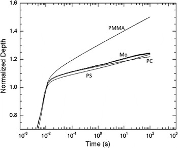
Normalized depth–time data for indents with 0.01-s load times are shown in Fig. 2 for each material tested. The depths increase smoothly with time during the creep hold. It is remarkable that in terms of normalized depth, Mo exhibits as much creep as both PS and PC. It turns out that all these materials possess very different viscoplastic behaviors, but those differences are easier to see in the area–time and hardness–indentation strain rate data than in the normalized depth–time data.
Normalized depth–time traces for each material with 0.01-s load times and 100-s creep hold times. The depths are normalized so that 1 corresponds to the end of the loading ramp and beginning of the creep hold, corresponding to time = 0.01 s.

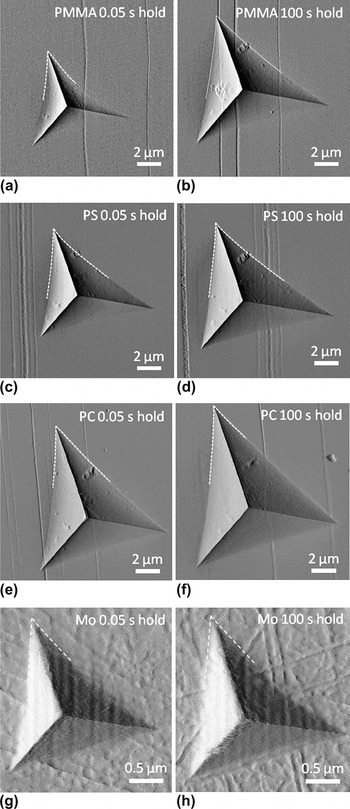
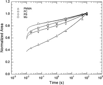
Continuous area–time curves are needed to generate instantaneous H and  . Increase in area during the creep hold was assessed by first measuring areas from AFM images of indents with different creep hold times (Fig. 3). Normalized area–time data from experiments with 0.01-s load times are shown in Fig. 4 for each material tested. Multiple data points for a given creep hold time correspond to measurements taken from indents with different unloading times. Next, the discrete area–time measurements were fit with continuous area–time curves constructed from nanoindentation load–depth–time traces using a physically based model,Reference Stone, Jakes, Puthoff and Elmustafa34 which is described in more detail in the “Appendix.” After area–time curves were constructed, Eqs. (1) and (2) were used to generate H and
 , respectively.
Atomic force microscopy (AFM) images of 10-mN indents with 0.05- and 100-s creep hold times in (a and b) poly(methylmethacrylate) (PMMA); (c and d) polystyrene (PS); (e and f) polycarbonate (PC); and (g and h) molybdenum (Mo). All indents had 0.01-s load and unload times. Dashed lines highlight the contact edges used to assess A 0. The identification of the contact edges for the polymers was described in detail in the accompanying article.Reference Jakes, Lakes and Stone28

Normalized area–time data from 100-s creep hold time for each material tested. The areas are normalized so that 1 corresponds to the area at the end of the 100-s creep hold time. The beginning of creep hold of the experiment is 0.01 s. The discrete points were measured from AFM images. The continuous curves were generated with the physically based modelReference Stone, Jakes, Puthoff and Elmustafa34 described in the “Appendix.”

B. Hardness–indentation strain rate
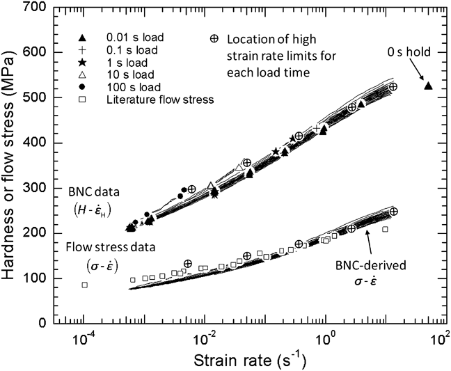
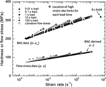
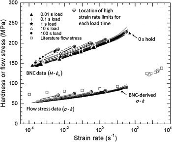
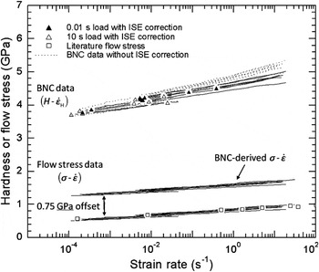
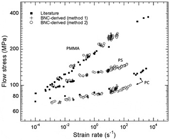
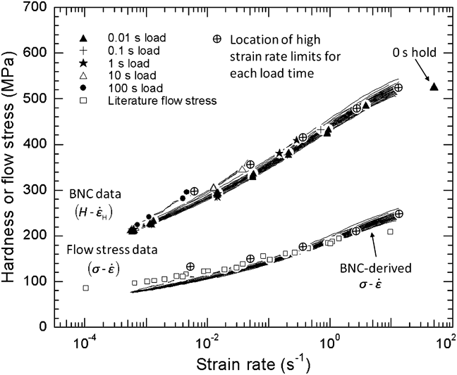
Experimental BNC hardness–indentation strain rate (H– ) data for PMMA, PS, PC, and Mo are shown in Figs. 5–8, respectively. Also included are compression flow stress–strain rate (σ–
 ) data taken from the literatureReference Swallowe and Lee42, Reference Richeton, Ahzi, Vecchio, Jiang and Adharapurapu44 and σ–
 converted from H–
 using method 1 described below. For now we will ignore the σ–
 data and are only concerned with the H–
 data in Figs. 5–8. BNC H–
 data with 0.01-s load times span strain rates between approximately 10−4 and 10 s−1, whereas experiments with longer load times span narrower ranges of strain rate because the creep portions of those experiments begin at lower strain rates. Also included in the polymer plots are H estimated from 0-s creep hold indents. These indents had 0.01-s load and unload times. Previous authorsReference Lucas and Oliver46 noted that the strain rate during a loading ramp is approximately
 , where
 is the rate of loading. Loading 10 mN in 0.01 s corresponds to a strain rate of approximately 50 s−1 immediately after the 0.01-s loading ramp, so these data are placed at this strain rate. The areas of indents with 0-s hold times likely grew irreversibly during unloading, so these values represent an approximate lower bound for H at this strain rate.
PMMA broadband nanoindentation creep (BNC) data (H– ) collected for load times ranging from 0.01 to 100 s. The high strain rate limits for each load time are represented by circles with cross hairs. Also included are two sets of flow stress data (σ–
 ): (i) literature σ–
 from uniaxial compression tests (Lee and SwalloweReference Swallowe and Lee42 and Richeton et al.Reference Richeton, Ahzi, Vecchio, Jiang and Adharapurapu44) and (ii) BNC-derived σ–
 calculated using the correlation in Fig. 9 following method 1 described in the “Discussion.”
PS BNC data (H– ) collected at load times ranging from 0.01 to 100 s. The high strain rate limits for each load time are represented by circles with cross hairs. Also included are two sets of flow stress data (σ–
 ): (i) literature σ–
 from uniaxial compression tests (Lee and SwalloweReference Swallowe and Lee42) and (ii) BNC-derived σ–
 calculated using the correlation in Fig. 9 following method 1 described in the “Discussion.”

PC BNC data (H– ) collected at load times ranging from 0.01 to 100 s. The high strain rate limits for each load time are represented by circles with cross hairs. Also included are two sets of flow stress data (σ–
 ): (i) literature σ–
 from uniaxial compression tests (Richeton et al.Reference Richeton, Ahzi, Vecchio, Jiang and Adharapurapu44) and (ii) BNC-derived σ–
 calculated using the correlation in Fig. 9 following method 1 described in the “Discussion.”

Mo BNC data (H– ) collected at load times of 0.01 and 10 s. In contrast to the polymers, Mo does not exhibit path dependence in H, but it does exhibit an indentation size effect (ISE) in H. Hardness–
 curves with the ISE correction [Eq. (4)] are plotted as solid lines, whereas the H–
 curves before ISE correction are plotted as dotted lines. Also included are three sets of flow stress data (σ–
 ): (i) literature σ–
 from uniaxial compression tests (Briggs and CampbellReference Briggs and Campbell45), (ii) BNC-derived σ–
 calculated using the correlation in Fig. 9 following method 1 described in the “Discussion,” and (iii) BNC-derived σ–
 offset by 0.75 GPa to account for differences in work hardening.

It can be seen from Figs. 5–7 that for the polymers, H– behavior depends on initial rate of loading. At fixed
 , the H is higher for slower loading rates. The fact that the properties depend on how they are measured means that they are path dependent. Path-dependent behavior is not observed in Mo (Fig. 8) nor in BNC of metallic glassesReference Puthoff, Jakes, Cao and Stone30 also tested at room temperature. We surmise that for the polymers, rate- and time-dependent structural changes take place during the loading ramp and that these changes affect the hardness during the subsequent creep hold. The observed behavior is likely related to the yield drop seen in compression tests of amorphous polymers.
The hardness in Mo exhibits an indentation size effect (ISE) [Fig. 1(a)]. Therefore, changes in H during indentation creep derive from changes in both strain rate and depthReference Stone and Yoder31 following

where mH is the strain rate sensitivity of the hardness ( ) and n measures the strength of the size effect. We measured n = −0.35 from the data in Fig. 1(a). Because of our interest in changes in H that derive solely from changes in
 , we subtract the second term on the right-hand side of Eq. (4) from experimental data to give H as a function of
 at fixed depth. Hardness–
 data with and without the correction for the indentation size effect are shown in Fig. 8.
IV. DISCUSSION
A. Conversion of hardness to flow stress
It is of interest to map BNC H– data onto literature σ–
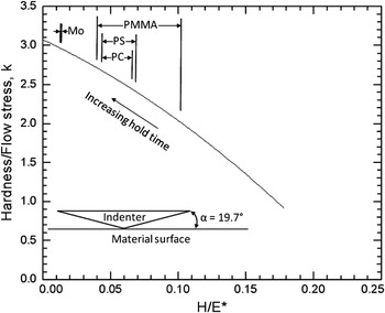
 data. Two methods produce satisfactory results. Both rely on the Tabor–Marsh–Johnson correlationReference Tabor47–Reference Johnson51 in which H = kσ and k is a function of indenter angle (α in Fig. 9) and E* / σ, where E* is the Hertzian contact modulus defined in Eq. (A2) of the “Appendix.” The difference between the two methods resides in how they convert strain rate. The first method is simpler: it assumes that
 , where
 is the strain rate for a uniaxial compression test and k′ is a constant, independent of hardness (we use k′ = 1). This method was proposed by Kermouche et al.Reference Kermouche, Loubet and Bergheau52, Reference Kermouche, Loubet and Bergheau53 and Elmustafa et al.Reference Elmustafa, Kose and Stone29 The second method, preferred by the latter authors because it does a better job of fitting finite element simulations, relaxes the assumption that k′ is constant. The two methods are virtually identical for low H / E* ratio where k′ = constant is a good approximation, and their difference increases as H / E* increases. For the second method,
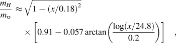
 can be generated by first taking mH and converting it to strain rate sensitivity of the flow stress (
 ) using the ansatz
The value of k as a function of H/E* for a Berkovich probe (cone equivalent α = 19.7°) based on analysis of the Tabor–Marsh–Johnson correlation.Reference Johnson51

where x = H / E*. The parameters used in Eq. (5) differ from the earlier versionReference Elmustafa, Kose and Stone29, Reference Puthoff, Jakes, Cao and Stone30 based on finite element analysis, although the difference does not drastically change the results. The new parameters have been motivated by discussions with A.A. Elmustafa (personal communication), who is modeling indentation creep for a variety of indenter geometries including Berkovich. In the earlier version, 0.21 was used as normalization for x inside the square root sign rather than 0.18, and 28.2 was used inside the arctangent function rather than 24.8 applied now. The value of x = 0.21 corresponds to the point at which mH / m σ → 0 and was obtained empirically based on finite element analysis. Not surprisingly, it turns out that x = 0.21 also corresponds to the fully elastic limit based on Sneddon’s theory,Reference Sneddon54 which gives H / E* = 0.202 indentation of an elastic solid with a 22° cone. The new expression therefore takes into account the difference between the cone angle (22°) for the simulations and equivalent cone angle (19.7°) for a Berkovich indenter. It assumes that both of the normalizing factors for x scale in proportion to tan α. Strain rate is obtained by integrating inverse strain rate sensitivity,
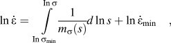
in which  is an integration constant with
 evaluated at the lowest hardness in the BNC experiment (H min), corresponding to the lowest stress, σmin. From Ref. Reference Elmustafa, Kose and Stone29, we estimate k′(σmin) = 2 for PMMA, 3.3 for PS, and 3.5 for PC.
The ratio k is shown in Fig. 9 for the Berkovich geometry and as a function of H / E*.Reference Puthoff, Jakes, Cao and Stone30 To convert H to σ, H / E* must be estimated at each point in the BNC data. The hardness is known, but for the polymers the moduli lack uniqueness because of viscoelasticity. We have yet to perform a systematic investigation of how best to deal with the viscoelastic modulus in this analysis. Nevertheless, the results are not too sensitive to the value of modulus chosen, and for the conversion here, we arbitrarily choose a value of E* that corresponds to the average measured from experiments with 1-s unloading time.Reference Jakes, Lakes and Stone28 The ranges of k values utilized for converting different BNC data are shown in Fig. 9.
The BNC-derived σ– curves constructed using method 1 are compared with literature σ–
 data in Figs. 5–8. For the polymers, the high strain rate limits of the BNC-derived σ–
 curves agree quite well with the literature data in Figs. 5–7. This is probably because the high strain rate data from BNC correspond to the beginning of the creep hold and to the behavior of the freshly deformed material, analogous to the onset of yielding in uniaxial compression, whereas the remainder of the creep hold, which agrees less well with the literature yield stress data, assesses properties affected by prior deformation, similar to the lower yield stress in a uniaxial compression experiment. The second method of converting BNC data tends to elongate the stress–strain rate data in the direction of strain rate (Fig. 10). The clearest difference in outcome between the two methods is for PC, where method 2 more accurately captures the upward curvature of the σ–
 data at high strain rates.
Comparison between BNC-derived σ– and literature uniaxial σ–
 data for the polymers. The BNC-derived σ–
 data calculated using both methods are included.

The same method for converting BNC data for polymers can be used for Mo. In this case k ≈ 3 (Fig. 9). In contrast to the BNC-derived σ– data for the polymers, the σ–
 data for Mo fall at higher levels of stress than the literature σ–
 data. This result is not surprising. Mo both work hardens and exhibits an indentation size effect, so we do not necessarily expect BNC-derived σ–
 to agree with literature σ–
 , which correspond to a different level of work hardening. Instead, the derivative
 , which is independent of work hardening,Reference Stone and Yoder31, Reference Briggs and Campbell45 agrees. When the nanoindentation-derived σ–
 data are offset downward in Fig. 8 by 0.75 GPa, they overlap the literature data.
B. Role of hydrostatic pressure in conversion of hardness to flow stress
Hydrostatic pressure is known to affect yielding in polymers,Reference Davis and Pampillo55–Reference Pae, Sauer, Silano, Timmerhaus and Barber57 which, for instance, is often modeled using Drucker–Prager or Mohr–Coulomb-type laws. A number of empirical and theoretical studies suggest that for materials that are sensitive to hydrostatic pressure, the ratio H/σ is increased. Reference Chen58–Reference Narasimhan62 In our analysis we have not directly accounted for hydrostatic stress but have relied solely on the empirical relationship shown in Fig. 9. However, much of the experimental data that went into constructing this relationship came from polymers like PMMA and PS.Reference Marsh49 In this case the pressure dependence of yielding in polymers is already implicitly included in the correlation.
C. Comparison of current PMMA results to previous work
We had previously tried the same comparison between BNC-derived σ– curves with literature σ–
 data for PMMA.Reference Puthoff, Jakes, Cao and Stone30 The agreement was rather poor and was attributed to effects of hydrostatic pressure. However, the older measurements were in error. As described in the accompanying article,Reference Jakes, Lakes and Stone28 we have reassessed the way we measure the areas of PMMA indents and have found we had previously underestimated the areas of indents with fast loading rates and short creep hold times. That error has been corrected here.
V. CONCLUDING REMARKS
BNC is used to generate hardness–indentation strain rate (H– ) data from amorphous polymers PMMA, PC, and PS and from the body-centered cubic metal Mo. A key part of the analysis is the ability to measure and accurately model the evolution of areas during the creep hold. Two slightly different methods were also used to convert H–
 data into BNC-derived σ–
 data. We found the following:
(1) BNC H–
 curves for PMMA, PS, and PC exhibit path dependence. The H– curves depend on the rate of loading preceding the creep hold.
(2) In contrast, BNC H–
curves for Mo do not exhibit path dependence. For Mo, the H– curves are independent of loading rate.(3) The BNC H–
data were converted to σ– data using two methods. Both methods rely on the Tabor–Marsh–Johnson correlation to convert H to σ. The first method assumes the is strictly proportional to , whereas with the second method the strain rate sensitivity of the hardness is converted to that of the flow stress, then the corresponding strain rates are obtained by integration. The two methods generate similar BNC-derived σ– data, but method 2 better replicates the behavior of the literature data for PC at high strain rates.(4) For the polymers, the high strain rate limits of the BNC-derived σ–
curves for each loading rate agree best with the literature σ– data. This means that it is necessary to perform experiments with different loading rates to generate σ– data from BNC data that will compare well with literature uniaxial σ– data. For Mo, the BNC-derived σ– data did not depend on loading rate and agree across the entire spectrum of strain rate. In this case, the σ– data can (at least in principle) be generated in a single BNC experiment.(5) In generating the BNC H–
curves, no assumptions are made about constitutive laws that govern the materials. It is nevertheless unmistakable that BNC-derived σ– curves reflect the viscoplastic properties of the materials.(6) The analyses to obtain BNC-derived σ–
curves rely on the ratio of H / E*. For the polymers, E* is not uniquely defined, so questions remain concerning how best to convert H to σ. Clearly, the overall approach is valid, but further details remain to be worked out.
 curves for PMMA, PS, and PC exhibit path dependence. The H–
 curves depend on the rate of loading preceding the creep hold.
 curves for Mo do not exhibit path dependence. For Mo, the H–
 curves are independent of loading rate.
 data were converted to σ–
 data using two methods. Both methods rely on the Tabor–Marsh–Johnson correlation to convert H to σ. The first method assumes the
 is strictly proportional to
 , whereas with the second method the strain rate sensitivity of the hardness is converted to that of the flow stress, then the corresponding strain rates are obtained by integration. The two methods generate similar BNC-derived σ–
 data, but method 2 better replicates the behavior of the literature data for PC at high strain rates.
 curves for each loading rate agree best with the literature σ–
 data. This means that it is necessary to perform experiments with different loading rates to generate σ–
 data from BNC data that will compare well with literature uniaxial σ–
 data. For Mo, the BNC-derived σ–
 data did not depend on loading rate and agree across the entire spectrum of strain rate. In this case, the σ–
 data can (at least in principle) be generated in a single BNC experiment.
 curves, no assumptions are made about constitutive laws that govern the materials. It is nevertheless unmistakable that BNC-derived σ–
 curves reflect the viscoplastic properties of the materials.
 curves rely on the ratio of H / E*. For the polymers, E* is not uniquely defined, so questions remain concerning how best to convert H to σ. Clearly, the overall approach is valid, but further details remain to be worked out.
ACKNOWLEDGMENTS
This work was supported by Cooperative Research and Development Agreement 10-RD-111111129-027 between Hysitron, Inc. and Forest Products Laboratory. Research was sponsored by the National Science Foundation (Award CMMI-0824719 to D.S. Stone).
APPENDIX
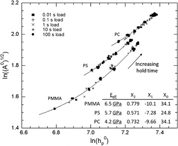
We obtain the continuous area–time curves in Fig. 4 by fitting continuous curves to the discrete area–time measurements also shown in the figure. Rather than relying on arbitrary functions like polynomials, power laws, or decaying exponentials to generate continuous area–time curves, we employ another approach that utilizes the nanoindentation load–depth–time traces. The method does a better job of capturing the trend of the data over a wide range of strain rate and has been validated and improved using finite element analysis.Reference Stone, Jakes, Puthoff and Elmustafa34 With this method it is assumed that  at constant load. The power law exponent ζp is used as a fitting parameter to fit the continuous area–time curve to the discrete experimental data. During the creep hold, hp is estimated using

where P is the instantaneous load (ideally, P = P 0 although in a real experiment P varies a small amount). The superscripts “0” refer to the values of the parameters at the end of the creep hold and  . E eff is given by

where E s and E d are Young’s moduli and νs and νd are Poisson’s ratios of specimen and indenter, respectively, and β ≈ 1.23.Reference Jakes, Frihart, Beecher, Moon and Stone36E* is the usual modulus encountered in Hertz contact problems. Equation (A1) is obtained from a theoretical analysis. However, for polymers E eff lacks uniqueness because of viscoelasticity, so the polymers do not strictly conform to the theory. In practice, this discrepancy does not present a problem because ζp is calculated using a representative value of E eff and in the end the continuous area–time curve is insensitive to the choice of E eff. Figure A1 shows ln (A0)1/2 versus  from experiments with different creep hold times at fixed load. The slopes of the curves correspond to ζp. Rather than forming straight lines, the data must be approximated as parabolas,

in which case  . PreviouslyReference Stone, Jakes, Puthoff and Elmustafa34 we had not been able to reliably detect that ζp varies with depth. However, our measurement methods are now better, and the finite element analyses neglected viscoelastic deformation, so it should come as no surprise that ζp is not a constant for the polymers.
Because ζp depends on hp, it is not straightforward to calculate hp using Eq. (A1). Therefore, to account for variation in ζp in Eq. (A1) we divide the raw depth–load–time data into 100 equal segments on a log(time) scale so that for each segment, ζp is approximately constant. We then analyze each segment separately starting with the final segment of the creep hold, where A= A 0 and  are known, and work backward to the beginning of the creep hold.
Data used to calculate ζp for PMMA, PS, and PC. For each material, data include indents with creep hold times that vary from 0.01 to100 s and load times that vary from 0.01 to 100 s. The 0.01-s load time data were fit to Eq. (A3), and these fits were differentiated to calculate ζp. The coefficients for the fit and the values of E eff used to calculate h p are given in the embedded table.