1 Introduction
Semantic similarity is the building block for numerous applications of natural language processing (NLP), such as grammar induction (Meng and Siu Reference Meng and Siu2002) and affective text categorization (Malandrakis et al. Reference Malandrakis, Potamianos, Iosif and Narayanan2011). Distributional semantic models (DSM) (Baroni and Lenci Reference Baroni and Lenci2010) are based on the distributional hypothesis of meaning (Harris Reference Harris1954) assuming that semantic similarity between words is a function of the overlap of their linguistic contexts. DSM are typically constructed from co-occurrence statistics of word tuples that are extracted from a text corpus or from data harvested from the web. A wide range of contextual features are also used by DSM exploiting lexical, syntactic, semantic, and pragmatic information. DSM have been successfully applied to the problem of semantic similarity computation. According to Baroni and Lenci (Reference Baroni and Lenci2010), the success of contextual DSM features is due to their ability to encode the attributes of word senses. According to attributional similarity (Turney Reference Turney2006), semantic similarity between words is based on the commonality of their sense attributes. A closely related assumption is that the semantic similarity between two words can be estimated as the similarity between their two closest senses (Resnik Reference Resnik1995), henceforth referred to as the maximum sense similarity assumption.
In this paper we investigate a new unsupervised approach for the construction of DSM with application to lexical semantic similarity computation. First, a corpus of snippets (short pieces of text containing words of interest) is harvested from the web. Then a semantic network is constructed encoding semantic relations between words in the corpus. Co-occurrence and context features are used to measure the strength of relations. The network is a parsimonious representation of the information encoded in the corpus. We then define the notion of semantic neighborhood and associated metrics of semantic similarity that exploit this notion. The proposed semantic similarity metrics are motivated by the maximum sense similarity, attributional similarity, and metric space assumptions. The similarity metrics are evaluated against human similarity ratings using standard datasets, achieving state-of-the-art results. This work builds upon our prior research in Iosif and Potamianos (Reference Iosif and Potamianos2010, Reference Iosif and Potamianos2012), while the following are the original contributions:
1. An efficient and scalable methodology is proposed for corpus creation using web-harvested data. Unlike the quadratic query complexity of our previous algorithm (Iosif and Potamianos Reference Iosif and Potamianos2010), the proposed method has linear query complexity with respect to the size of the lexicon.
2. Three unsupervised language-agnostic similarity computation algorithms are proposed that exploit the semantic neighborhoods. The best performing neighborhood-based metrics outperform well-established approaches that rely on elaborate knowledge resources.
3. We demonstrate the effectiveness of co-occurrence-based similarity metrics when corpus-based frequencies are incorporated in comparison to the use of web hits (Iosif and Potamianos Reference Iosif and Potamianos2010). This is further investigated with respect to the textual proximity of co-occurring words.
4. The assumption that the semantic similarity between two words can be estimated as the similarity between their two closest senses is validated using (sense-untagged) web data.
5. The computation of semantic neighborhoods introduced in Iosif and Potamianos (Reference Iosif and Potamianos2012) is extended by applying a number of co-occurrence-based similarity metrics in addition to the context-based metrics. Word co-occurrence is shown to be more salient than contextual features regarding the discovery of senses via semantic neighborhoods.
The remainder of the work is organized as follows: In Section 2, we review related work in the areas of semantic similarity computation and word sense disambiguation. In Section 3 co-occurrence and context-based similarity metrics are reviewed. The procedure and motivation behind harvesting a corpus of snippets from the web is detailed in Section 4. In Section 5, we define our semantic network and propose three novel similarity metrics that utilize the notion of semantic neighborhood. The corpora and experimental procedures are described in Section 6, while the evaluation results are reported in Section 7. Last, Section 8 concludes this work.
2 Related work
Semantic similarity metrics can be divided into two broad categories: (i) Metrics that rely on knowledge resources, and (ii) corpus- or web-based metrics that do not require any external knowledge source. A representative example of the first category are metrics that exploit the WordNet ontology (Miller Reference Miller1990). For computing word similarity, these metrics incorporate features such as the length of paths between them (Wu and Palmer Reference Wu and Palmer1994; Leacock and Chodorow Reference Leacock, Chodorow and Fellbaum1998) or the information content of their least subsumer that is estimated from a corpus (Resnik Reference Resnik1995; Jiang and Conrath Reference Jiang and Conrath1997). WordNet glosses have been also exploited for extracting contextual information (Banerjee and Pedersen Reference Banerjee and Pedersen2002; Patwardhan and Pedersen Reference Patwardhan and Pedersen2006). An in-depth review of major WordNet-based metrics can be found in Budanitsky and Hirst (Reference Budanitsky and Hirst2006). Corpus-based metrics are formalized as DSM (Baroni and Lenci Reference Baroni and Lenci2010) and are based on the distributional hypothesis of meaning (Harris Reference Harris1954). DSM can be categorized into unstructured (unsupervised) that employ a bag-of-words model (Iosif and Potamianos Reference Iosif and Potamianos2010) and structured that rely on syntactic relationships between words (Grefenstette Reference Grefenstette1994; Baroni and Lenci Reference Baroni and Lenci2010).
The core idea behind structured models is the utilization of syntactic relationships as features for the creation of semantic spaces. Typical examples of such relations are argument structures (subject/object) and modifications (adjective–noun) extracted by shallow or full parsing (Padó and Lapata Reference Padó and Lapata2007). Syntactic relations can be represented as two-tuples of the arguments (Grefenstette Reference Grefenstette1994) or as n-tuples in order to incorporate direct and indirect dependencies (Padó and Lapata Reference Padó and Lapata2007). The paradigm of ‘one task, one model’ of structured DSM was advanced in Baroni and Lenci (Reference Baroni and Lenci2010) by the arrangement of tuples into a third-order tensor. This enables the creation of different semantic spaces for different semantic tasks (e.g. estimation of semantic similarity between words, categorization of concepts, computation of verb selectional preferences, etc.), while the extraction of dependency tuples is task-independent (‘the same distributional information can be shared across tasks’). The performance of knowledge-based metrics and DSM for the problem of semantic similarity estimation between words was compared in Agirre et al. (Reference Agirre, Martínez, de Lacalle and Soroa2006). Unstructured DSM were shown to obtain slightly higher performance than structured ones, where knowledge-based and DSM approaches yielded comparable results. The best performance was obtained using a supervised combination of a knowledge-based (WordNet) approach and two variations of unstructured DSM.
Exemplar models were proposed as an alternative implementation of DSM for addressing the problem of polysemy (Erk and Padó Reference Erk and Padó2010; Reddy et al. Reference Reddy, Klapaftis, McCarthy and Manandhar2011). Instead of a single vector, a set of exemplars is utilized for the representation of a target word. The set of exemplars is defined as the set of (corpus) sentences in which the target occurs (Erk and Padó Reference Erk and Padó2010). Each exemplar can be represented as a structured (i.e. bag-of-words) or unstructured (i.e. encoding syntactic relations) vector. For a target word given within context (e.g. sentential) polysemy is modeled by the activation/selection of relevant exemplars with respect to a ‘point of comparison’, where the latter can be regarded as another exemplar (Erk and Padó Reference Erk and Padó2010). A related example is the selection of paraphrases for a target word that occurs in a given context (Erk and Padó Reference Erk and Padó2010). In Reddy et al. (Reference Reddy, Klapaftis, McCarthy and Manandhar2011), the exemplar model was applied in the framework of semantic compositionality for the task of similarity computation between noun–noun compounds.
Web-based metrics employ search engines to estimate the frequency of word co-occurrence (Turney Reference Turney2001; Vitanyi Reference Vitanyi2005; Gracia et al. Reference Gracia, Trillo, Espinoza and Mena2006) or construct corpora (Bollegala, Matsuo and Ishizuka Reference Bollegala, Matsuo and Ishizuka2007; Iosif and Potamianos Reference Iosif and Potamianos2010). The identification and extraction of other types of relations has been mainly studied through the use of linguistic patterns. Lexico-syntactic patterns were applied in the influential work of Hearst (Reference Hearst1992) for the identification of hyponymy, followed by numerous similar approaches, e.g. Caraballo (Reference Caraballo1999).
Recently, motivated by the graph theory, several aspects of human languages have been modeled using network-based methods. In Radev and Mihalcea (Reference Radev and Mihalcea2008) and Mihalcea and Radev (Reference Mihalcea and Radev2011), an overview of network-based approaches is presented for a number of NLP problems. Different types of language units can be regarded as vertices of such networks, spanning from single words to sentences. Typically, network edges represent the relations of such units capturing phenomena such as co-occurrence, syntactic dependencies, and lexical similarity. An example of a large co-occurrence network is presented in Widdows and Dorow (Reference Widdows and Dorow2002) for the automatic creation of semantic classes. In Ferrer-I-Cancho and Solé (Reference Ferrer-I-Cancho and Solé2001), it is reported that the co-occurrence networks of words that co-exist at very short proximity exhibit a number of small-world properties and are highly clustered. Similar observations regarding the structural properties of co-occurrence networks were also made in Véronis (Reference Véronis2004), where the HyprLex algorithm was proposed for sense discovery. In Agirre et al. (Reference Agirre, Martínez, de Lacalle and Soroa2006), an extension of the main ideas presented in Véronis (Reference Véronis2004) was proposed for word sense disambiguation (WSD). In particular, the PageRank algorithm (Brin and Page Reference Brin and Page1998) was employed for identifying hubs over a co-occurrence network.
Semantic similarity computation is closely related to WSD. WSD methods can be divided into two main categories: (i) supervised approaches that apply machine learning for learning sense labels for a set of words with respect to a given context (sense labeling), and (ii) unsupervised approaches that automatically discriminate (discover) word senses without label assignment. A detailed survey of WSD is provided in Ide and Vèronis (Reference Ide and Véronis1998), Agirre and Edmonds, (Reference Agirre and Edmonds2007), and Navigli (Reference Navigli2009) . The employment of network-based metrics for the computation of semantic similarity has attracted less attention compared to WSD. WordNet-based similarity metrics can be regarded as a special case of network metrics, since they are built on the top of a manually created network. To the best of our knowledge few network-based metrics are reported in the literature that integrate network creation with semantic similarity computation. In Lemaire and Denhière (Reference Lemaire and Denhière2004), a co-occurrence network was constructed, and the similarity between two words was estimated as the product of weights of the shortest path between them with moderate performance results.
Other network-based approaches rely on the use of linguistic tools and/or knowledge resources. In Harrington (Reference Harrington2010), a semantic network was created from a corpus using a set of tools for named entity recognition, parsing, and semantic analysis. The similarity between words (nodes) was estimated according to an implementation of the spreading activation model (Collins and Loftus Reference Collins and Loftus1975). Wikipedia articles were exploited by the WikiRelate! system (Strube and Ponzetto Reference Strube and Ponzetto2006) in conjunction with the corresponding category tree for the creation of a semantic network. In Hughes and Ramage (Reference Hughes and Ramage2007), an approach based on random walks was applied over WordNet for estimating word similarity. WordNet was also used in Agirre et al. (Reference Agirre, Martínez, de Lacalle and Soroa2006) where the personalized PageRank algorithm (Haveliwala et al. Reference Haveliwala, Gionis, Klein and Indyk2002) was applied for the computation of a probability distribution for every target word. Word similarity was estimated via the cosine similarity between vectorized distributions.
Following the paradigm of the vector space model (VSM) that constitutes the main implementation of DSMs, our approach is based on corpus-based co-occurrence statistics for the creation of a semantic network. One important difference with prior work in this area is that no language-specific tools, e.g. dependency parsers (Baroni and Lenci Reference Baroni and Lenci2010), or human annotations, e.g. Wikipedia hyperlinks (Wojtinnek, Pulman and Völker Reference Wojtinnek, Pulman and Völker2012), are used here. For example, in Wojtinnek et al. (Reference Wojtinnek, Pulman and Völker2012) the English Wikipedia was used for the disambiguation of target words (Wikipedia concepts), and a very large network was constructed by exploiting the hyperlinks between them. For each node (word) a vector was created, including a number of strongly connected nodes selected by an algorithm inspired by spreading activation theory (Collins and Loftus Reference Collins and Loftus1975). The similarity between two words was estimated as the cosine of their respective vectors. In our work, two types of metrics are investigated for weighting the strength of the link between a reference noun and its neighbors, namely co-occurrence-based and context-based. Co-occurrence-based metrics were previously used for the weighting of contextual features (Agirre et al. Reference Agirre, Alfonseca, Hall, Kravalova, Pasca and Soroa2009; Baroni and Lenci Reference Baroni and Lenci2010) and the creation of co-occurrence networks (Widdows and Dorow Reference Widdows and Dorow2002). To the best of our knowledge, context-based metrics have never been applied for any of the aforementioned tasks. Our work is also motivated by cognitive consideration and theories of semantics. The network-based metrics proposed here are motivated by two well-founded hypotheses regarding semantic similarity, namely maximum sense similarity (Resnik Reference Resnik1995) and attributional similarity (Turney Reference Turney2006). Our work extends the traditional VSM approach into a two tier system: Corpus statistics are parsimoniously encoded in a network, while the task of similarity computation is shifted (from corpus-based techniques) to operations over network neighborhoods. The proposed network creation process constitutes a new paradigm for implementing DSMs that enables the direct exploitation of neighborhood semantics, e.g. definition of metrics that adopt different hypotheses regarding semantic similarity, investigation of neighborhood structural properties.
3 Similarity metrics
Next, the two main types of similarity metrics used in this paper are presented, namely co-occurrence and context-based metrics.
3.1 Co-occurrence-based metrics
The underlying assumption of co-occurrence-based metrics is that two words that co-exist in the same web document are semantically related. Let {M} be the entire set of web documents indexed by a search engine. A set of documents returned by a search engine for query words wi, . . ., w i + n is denoted as {M; wi, . . ., w i + n}, with cardinality |M; wi, . . ., w i + n|. The latter is also known as the number of hits for the submitted query. In this work, we employ four co-occurrence-based similarity metrics defined next (Iosif and Potamianos Reference Iosif and Potamianos2010).
Jaccard coefficient: In general, this coefficient computes the similarity between sets. In our case, we consider the sets of web documents that are indexed by the words of interest. The Jaccard coefficient J between words wi and wj is defined as follows:
 \begin{equation}
\mbox{$J(w_{i},w_{j})$} = \frac{\mid \!M;{w_{i},w_{j}}\!\mid }{\mid \!M;w_{i}\!\mid + \mid \!M;w_{j}\!\mid -\mid \!M;w_{i},w_{j}\!\mid }
\end{equation}
The Jaccard coefficient takes value between 0 (totally dissimilar) and 1 (totally similar).
Dice coefficient: This coefficient is closely related to the Jaccard coefficient and it is defined as follows:
 \begin{equation}
\mbox{$D(w_{i},w_{j})$}=\frac{2\mid \!M;w_{i},w_{j}\!\mid }{\mid \!M;w_{i}\!\mid +\mid \!M;w_{j}\!\mid }
\end{equation}
As before, D ranges between 0 and 1 for absolute dissimilarity and similarity, respectively.
Mutual information: Assuming that |M; wi|, |M; wj| are random variables, then their point-wise mutual information reflects the dependence between the occurrence of wi and wj as follows (Bollegala et al. Reference Bollegala, Matsuo and Ishizuka2007):
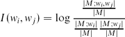 \begin{equation}
\mbox{$I(w_{i},w_{j})$}= \log \frac{\frac{\mid M;w_{i},w_{j} \mid }{\mid M \mid }}{ \frac{\mid M;w_{i} \mid }{\mid M \mid } \frac{\mid M;w_{j} \mid }{\mid M \mid } }
\end{equation}
The mutual information is unbounded ranging from positive to negative values as the similarity between words decreases.
Google-based semantic relatedness: The ‘normalized Google distance’ was proposed in Vitanyi (Reference Vitanyi2005), defined as follows:
 \begin{equation}
\mbox{$G_{0}(w_{i},w_{j})$}= \frac{\max \lbrace \log \mid \!M;w_{i}\!\mid , \log \mid \!M;w_{j}\!\mid \rbrace -\log \mid \!M;w_{i},w_{j}\!\mid }{\log \mid \!M\!\mid -\min \lbrace \log \mid \!M;w_{i}\!\mid , \log \mid \!M;w_{j}\!\mid \rbrace }
\end{equation}
This metric is a dissimilarity measure, i.e. as the semantic similarity between two words increases the metric takes smaller values. The scores assigned by (4) are unbounded, ranging from 0 to ∞. In Gracia et al. (Reference Gracia, Trillo, Espinoza and Mena2006), a variation of the normalized Google distance was used, proposing a bounded similarity measure called ‘Google-based semantic relatedness’, defined as
 \begin{equation}
\mbox{$G(w_{i},w_{j})$}= e^{-2\mbox{$G_{0}(w_{i},w_{j})$}}
\end{equation}
G 0(wi, wj) is computed according to (4). The Google-based semantic relatedness is bounded in [0,1].
Besides the use of the web as a corpus for obtaining number of hits, the aforementioned co-occurrence-based metrics can be also defined with respect to any text corpus. In such cases, the word frequencies can be considered at the level of several corpus units, e.g. sentences, paragraphs. In this work, we adopt both perspectives, i.e. employing web-based hits as well as word frequencies computed over a text corpus (see Section 7.1). Beyond computing similarities at the word level, the proposed metrics have been also shown to perform well for phrase-level similarity tasks. In Malandrakis, Iosif and Potamianos (Reference Iosif and Potamianos2012), a parametric version of mutual information using the corpus creation method proposed here was integrated in a sentence-level model with good results.
3.2 Context-based metrics
The fundamental assumption behind context-based metrics is that similarity of context implies similarity of meaning: we expect that words that share similar lexical contexts will be semantically related (Harris Reference Harris1954). A common representation of contextual features is the ‘bag-of-words’ model that assumes independence between features (Sebastiani and Ricerche Reference Sebastiani and Ricerche2002).
For context-based metrics, a contextual window of size 2H + 1 words is centered on the word of interest wi and lexical features are extracted. For every instance of wi in the corpus, the H words left and right of wi are taken into consideration, i.e.
 \begin{equation*}
[f_{H,l} \ldots f_{2,l} f_{1,l}] w_i [f_{1,r} f_{2,r} \ldots f_{H,r}]
\end{equation*}
where f k, l and f k, r represent the feature k positions to the left of right of wi. For a given value of H, the feature vector for wi is built as T wi, H = (t wi, 1, t wi, 2, . . ., t wi, Z), where t wi, k is a non-negative integer. The feature vector has length equal to the vocabulary size Z. Non-zero feature value t wi, k indicates the occurrence of vocabulary word tk within the left or right context of wi. Note that the value of t wi, k is set by considering all occurrences of wi in the corpus. The value of t wi, k can be defined according to a binary schemeFootnote 1 (Iosif and Potamianos Reference Iosif and Potamianos2010). This scheme assigns 1 to t wi, k if vocabulary word tk occurs within H positions left or right of word wi, otherwise, t wi, k = 0. The context-based semantic similarity metric QH between words wi and wj is computed as the cosine of their feature vectors:
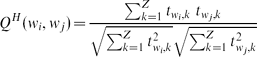 \begin{equation}
Q^{H}(w_i,w_j) \! = \! \frac{\sum _{k=1}^{Z}t_{w_i,k} \; t_{w_j,k}}{\sqrt{\sum _{k=1}^{Z}t_{w_i,k}^2} \sqrt{\sum _{k=1}^{Z}t_{w_j,k}^2}}
\end{equation}
for context size H and vocabulary size Z. For words wi, wj that share no common context (completely dissimilar words) the corresponding semantic similarity score is 0. Also, QH(w, w) = 1.
4 Corpus creation using targeted web queries
In this section we investigate the creation of corpora from web-harvested data via the formulation of targeted queries. There are two main types of web queries that can be used for corpus creation: (i) conjunctive queries (AND), and (ii) individual queries (IND).Footnote 2
Assuming N words in our lexicon, in the first case all pairwise AND conjunctions are formed and the corresponding queries are posed to a web engine, e.g. ‘wi AND wj’. Corpus creation via AND queries leads to quadratic query complexity  ${\cal O}(N^2)$ in the number of words in the lexicon. Alternatively, one can download documents or snippets with linear query complexity
 ${\cal O}(N)$ using IND queries, i.e. ‘wi’.
The main advantage of AND queries is that they construct a corpus that is conditioned on word-pairs, explicitly requesting the co-occurrence of word-pairs in the same document. Co-occurrence is a strong indicator of similarity, and corpora created via AND queries have been shown to provide very good semantic similarity estimates (Iosif and Potamianos Reference Iosif and Potamianos2010). To better understand the role of co-occurrence as a feature in semantic similarity computation, we need to revisit the very definition of semantic similarity, as it pertains to words and their senses. According to the information-theoretic approach proposed in Resnik (Reference Resnik1995), the similarity between two concepts can be estimated as the similarity between their two closest senses. This is also in agreement with our ‘common sense’ (cognitive) model of semantic similarity: when two words are mentioned, their closest senses are activated.Footnote 3 We believe that an important contribution of the co-occurrence feature to semantic similarity computation is that co-occurrence acts as a semantic filter that only retains the two closest senses. See Section 7.2 for the experimental justification of this claim.
Unfortunately, attempting to build corpora and DSM using conjunctive AND queries does not scale to thousands of words due to quadratic query complexity.Footnote 4 We are thus forced to investigate the alternative of using IND queries and face the sense disambiguation issues associated with such corpora. Corpora created via IND queries are similar to a typical text corpus with one important difference: the frequency of occurrence of the words in our lexicon can be manipulated to deviate from Zipf’s law. Assuming that the same number of snippets is downloaded for each word in our lexicon (using IND queries), we expect that rare words will be well represented within the corpus. As a result, the corpus will be more ‘informative’, i.e. the entropy rate of a unigram (zeroth order Markov process) model will be higher.
The normalization word-frequency effect can be illustrated by plotting the empirical distribution of the frequency of the words in the lexicon. Using a lexicon of 8752 nouns, the noun frequencies are plotted as a function of their rank in Figure 1. More specifically, we created a web corpus by posing an IND query for each noun and retrieving the 1000 top-ranked snippets (see Section 6). The corpus frequencies were multiplied by 104 to facilitate the comparison with the red curve showing web hits frequency. According to Zipf’s law (Zipf Reference Zipf1965), the frequency of a word w decreases non-linearly as its rank increases:
 \begin{equation}
f(w) = \frac{c}{r(w)^{\gamma }}
\end{equation}
where f(w) and r(w) are the frequency and the rank of word w, respectively, while c and γ are corpus-dependent. It is clear that the frequency difference between the high-ranked and the low-ranked words is somewhat normalized, i.e. smaller (absolute) γ, for the case of corpus frequencies as opposed to the use of web hits. For the example of Figure 1, γ equals to − 0.54 and − 0.90 for corpus frequencies and web hits, respectively. These values were computed for the ranks lying between 1000 and 6000 using a least squares linear model. This normalization is expected to smooth the domination of very frequent words at the denominator of co-occurrence-based metrics, such as (1)–(3). The performance of web hits and corpus counts is presented in Table 2.
Frequency of 8,752 nouns versus their rank. The frequencies were computed using (1) corpus counts (black curve), and (2) web hits (red curve). For comparison purposes the corpus frequencies were multiplied by 104.

5 Semantic network
Next we construct a semantic network encoding the relevant corpus statistics. The network is defined as an undirected (under a symmetric similarity metric) graph F = (V, E) whose set of vertices V are all words in our lexicon L, and the set of edges E contains the links between the vertices. The links (edges) between words in the network are determined and weighted according to the pairwise semantic similarity of the vertices.
The network is a parsimonious representation of corpus statistics as they pertain to the estimation of semantic similarities between word-pairs in the lexicon. In addition, the network can be used to discover relations that are not directly observable in the data; such relations emerge via the systematic covariation of similarity metrics. Semantic neighborhoods play an important role in this process. The members of the semantic neighborhoods of words are expected to contain features capturing diverse information at the syntactic, semantic, and pragmatic levels.
5.1 Semantic neighborhoods
For each word (reference word) that is included in the lexicon, wi ∈ L, we consider a subgraph of F, Fi = (Ni, Ei), where the set of vertices Ni includes in total n members of L, which are linked with wi via edges Ei. The Fi subgraph is referred to as the semantic neighborhood of wi (Iosif and Potamianos Reference Iosif and Potamianos2012). The members of Ni (neighbors of wi) are selected according to a semantic similarity metric (co-occurrence-based defined in Section 3.1, or context-based defined in Section 3.2) with respect to wi, i.e. the n most similar words to wi are selected. Note that the semantic network is not a metric space under (the proposed co-occurrence or context-based) semantic similarity because the triangle inequality is, in general, not satisfied. Next, we propose three semantic similarity metrics that utilize the notion of semantic neighborhood.
5.2 Maximum similarity of neighborhoods
This metric is based on the hypothesis that the similarity between two words, wi and wj, can be estimated by the maximum similarity between their respective sets of neighbors defined as follows:
 \begin{equation}
M_{n}(w_i,w_j)= \max \lbrace \alpha _{ij},\alpha _{ji}\rbrace
\end{equation}
where
 \begin{equation*}
\alpha _{ij} = \max _{x \in N_j}S(w_i,x), \alpha _{ji} = \max _{y \in N_i}S(w_j,y)
\end{equation*}
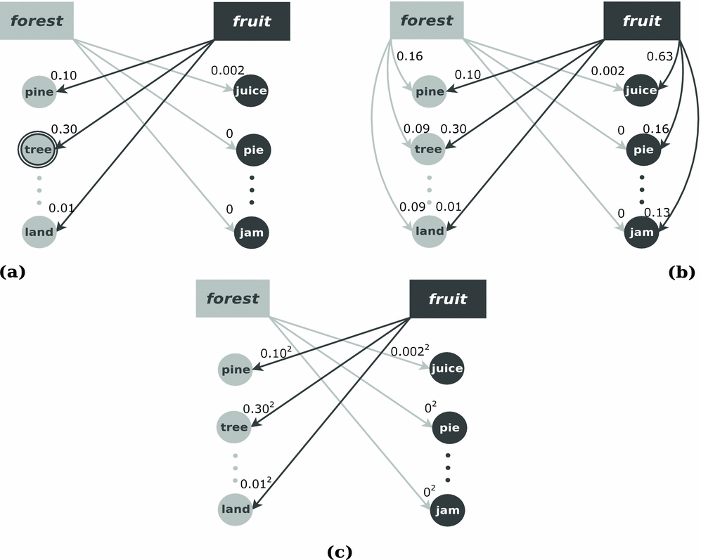
αij (or αji) denotes the maximum similarity between wi (or wj) and the neighbors of wj (or wi) that is computed according to a similarity metric S (see for example (1)–(3), (5), and (6)). Ni and Nj are the set of neighbors for wi and wj, respectively. The definition of Mn is motivated by the maximum sense similarity assumption.Footnote 5As discussed above, semantic neighborhoods encode diverse information. Here the underlying assumption is that the most salient information in the neighbors of a word are semantic features denoting senses of this word. In other words, we assume that semantic neighborhoods (and semantic networks, in general) can be used to mine for word senses.Footnote 6The Mn metric takes values in the interval [0, 1], where 1 stands for absolute similarity. Also, Mn(wi, wj) = Mn(wj, wi), i.e. Mn is symmetric. An example illustrating the computation of similarity between ‘forest’ and ‘fruit’ is depicted in Figure 2(a).  $M_{n}(\it{`forest'}, \it{`fruit'})=0.30$ because the similarity between ‘fruit’ and ‘tree’ (among all neighbors of ‘forest’) is the largest.
Pictorial view of neighborhood-based metrics. Two reference nouns, ‘forest’ and ‘fruit’, are depicted along with their neighborhoods: {pine, tree,..., land} and {juice, pie,..., jam}, respectively. Arcs represent the similarities between reference nouns and neighbors. The similarity between ‘forest’ and ‘fruit’ is computed according to (a) maximum similarity of neighborhoods, (b) correlation of neighborhood similarities, and (c) sum of squared neighborhood similarities.
5.3 Correlation of neighborhood similarities
The similarity between wi and wj is defined as follows:
 \begin{equation}
R_{n}(w_i,w_j) = \max \lbrace \beta _{ij}, \beta _{ji}\rbrace
\end{equation}
where
 \begin{equation*}
\beta _{ij} = \rho \left(C_{i}^{N_{i}},C_{j}^{N_{i}}\right), \beta _{ji}=\rho \left(C_{i}^{N_{j}},C_{j}^{N_{j}}\right)
\end{equation*}
and
 \begin{equation*}
C_{i}^{N_{i}}= (S(w_{i},x_{1}),S(w_{i},x_{2}),\ldots ,S(w_{i},x_{n}))\quad {\rm where} N_{i}=\lbrace x_{1},x_{2},\ldots ,x_{n}\rbrace
\end{equation*}
Note that C Nij, C Nji, and C Njj are defined similarly as C Nii. The ρ function stands for the Pearson’s correlation coefficient, Ni is the set of neighbors of word wi, and S is a similarity metric. Here we aim to exploit the entire semantic neighborhoods for the computation of semantic similarity as opposed to Mn where a single neighbor is utilized. The motivation behind this metric is attributional similarity, i.e. we assume that semantic neighborhoods encode attributes (or features) of a word. Neighborhood correlation similarity in essence compares the distribution of semantic similarities of the two words on their semantic neighborhoods. Thus, this metric is expected to provide more robust similarity estimates compared to Mn, especially when few data are available. The ρ function incorporates the covariation of the similarities of wi and wj with respect to the members of their semantic neighborhoods. The underlying assumption is that two semantically similar words are expected to have co-varying similarities with respect to their neighbors. Moreover, the ρ function normalizes this covariance by the standard deviations of the similarities of wi and wj. The similarity scores computed by Rn metric ranges in the interval [ − 1, 1], where − 1 and 1 denote zero and absolute similarity, respectively. Rn is symmetric, since Rn(wi, wj) = Rn(wj, wi). The similarity computation process is exemplified in Figure 2(b) for the words w 1 = ‘forest’ and w 2 = ‘fruit’. The similarity vectors between the neighbors N 1 of ‘forest’ and each of the words are computed: C N 11 = (0.16, 0.09, . . ., 0.09), C N 12 = (0.10, 0.30, . . ., 0.01). Similarly, C N 21, C N 22 are computed for the neighbors of ‘fruit’ and combined to estimate  $R_{n}(\it{`forest'}, \it{`fruit'})=-0.04$.
5.4 Sum of squared neighborhood similarities
The similarity between wi and wj is defined as follows:
 \begin{equation}
E_{n}^{\theta }(w_i,w_j) = \Bigg ( \sum _{x \in N_j} S^{\theta }(w_i,x) + \sum _{y \in N_i} S^{\theta }(w_j,y) \Bigg )^{\frac{1}{\theta }}
\end{equation}
where Ni is the set of neighbors of word wi, and S is any similarity metric. Similar to (9), all neighbors contribute to the computation of the final similarity score, here this is performed by summing the squares (θ = 2) of similarities between wi and wj’s neighbors. The same calculation is repeated for wj and the neighbors of wi to make E θn(wi, wj) symmetric. This is illustrated in Figure 2(c) for the computation of similarity between ‘forest’ and ‘fruit’ for θ = 2. That is  $E_{n}^{\theta =2}(\it{`forest'}, \it{`fruit'})= \sqrt{(0.10^2+0.30^2+\cdots +0.01^2)+(0.002^2+0^2+\cdots +0^2)}$ = 0.22. The E θ = 2n metric is unbounded since the yielding similarity scores range within [0, ∞). This range is smoothed in a nonlinear way by taking the square root of the accumulated squares of similarities. As in (9), the motivation underlying E θ = 2n metric is the attributional similarity, i.e. neighbors stand as attributes (or features). However, what is different here is the utilization of the attributional similarity as indicator for semantic similarity, i.e. the accumulation of word-to-neighbor similarities. The contribution of each word-to-neighbor similarity is nonlinearly weighted using the square of the respective similarity score. The motivation behind using θ > 1 is that more similar words in the neighborhoods should be weighted more in the final similarity decision.Footnote 7Qualitatively, the E θ = 2n weighting scheme takes the middle road between selecting the maximum pairwise similarity in (8) and the ‘linear’ weighting of pairwise similarity in (9). Note that as θ goes to ∞, E θn and Mn become equivalent.
6 Evaluation datasets, corpora, and experimental procedure
6.1 Evaluation datasets
The performance of similarity metrics was evaluated against human ratings from three standard datasets of noun pairs, namely (1) MC (Miller and Charles Reference Miller and Charles1998), (2) RG (Rubenstein and Goodenough Reference Rubenstein and Goodenough1965), and (3) WS353 (Finkelstein et al. Reference Finkelstein, Gabrilovich, Matias, Rivlin, Solan, Wolfman and Ruppin2002). The first dataset consists of twenty-eight noun pairs. For the second and the third dataset we present results for the subset of fifty-seven and 272 pairs, respectively, that are also included in SemCor3Footnote 8 corpus. The Pearson’s correlation coefficient was used as evaluation metric to compare estimated similarities against the ground truth. Let X = (x 1, x 2, . . ., xm) and Y = (y 1, y 2, . . ., ym) be the vectors that contain the similarity scores given by human subjects and the computational metric, respectively, for each of the i = 1, 2, . . ., m word pairs of the datasets. Pearson’s correlation coefficient is computed as follows:
 \begin{equation*}
\rho _{xy}= \frac{\sum ^{m}_{i=1} (x_{i}-\bar{x}) (y_{i}-\bar{y})}{\sqrt{\sum ^{m}_{i=1} (x_{i}-\bar{x})^2 \sum ^{m}_{i=1} (y_{i}-\bar{y})^2}}
\end{equation*}
where  $\bar{x}$ and
 $\bar{y}$ are the sample means of X and Y, for i = 1, 2, . . ., m. This coefficient was selected instead of Spearman’s rank correlation coefficient to retain the initial scaling of similarities in the evaluation metric, as opposed to the alternation of this scaling through the transformation of similarities into ranks.
6.2 Experimental corpora and procedure
We created the following corpora of web snippets using AND or IND queries posed via the Yahoo! Search API: (1) Corpus1: Using AND queries 1, 000 snippets were acquired for each pair of nouns, for the MC dataset. The major aspect of this corpus is the (explicitly requested) co-occurrence of nouns for which the similarity is computed. (2) Corpus2: Using IND queries 1, 000 snippets were acquired for each (unique) noun of the MC dataset. Unlike Corpus1, the creation of Corpus 2 is not driven by the co-occurrence constraint. (3) Corpus3: The same IND queries were used as for the case of Corpus2, but the queries were augmented with lexical descriptors denoting senses (see Section 7.2 for details). Corpus3 can be regarded as an extension of Corpus2, in which the acquired data are intended to (uniformly) cover different senses of nouns. The aforementioned corpora are exploited (see Section 7.2) for investigating the effect of word co-occurrence and their senses to the computation of context-based similarity (for the MC dataset only). (4) Corpus4: This is a corpus created using IND queries, consisting of approximately 8, 752, 000 snippets. More specifically, 1, 000 snippets were acquired for each noun taken from a set of 8, 752 English nouns of the SemCor3 corpus. Corpus4 is used for the creation of the semantic network as described in Section 5.
For Corpus4 the baseline performance of co-occurrence and the context-based similarity metrics were computed (see also parameter definition). Then the semantic neighborhoods were defined and the maximum/correlation neighborhood similarities were computed. A detailed list of experiments was conducted trying to investigate the performance of the following list of parameters: (1) the size of the contextual window, H, used in QH, Mn, Rn, E θ = 2n; (2) the metric used for the selection of neighbors: co-occurrence-based (J, D, I, G) or context-based similarity (QH); (3) the S metric used in Mn, Rn, E θ = 2n: co-occurrence-based (J, D, I, G) or context-based similarity (QH); (4) the neighborhood size (number of neighbors n) used in Mn, Rn, E θ = 2n metrics; (5) the corpus size, i.e. number of snippets per word (50, 100, 200, 500, 1,000) used to construct the network; and (6) the network size, that is, the number of concepts (nouns of lexicon) that constitutes the network: 9, 88, 176, 876, 1,751, 4,376, 6,127, and 8,752. The results are presented next.
7 Results
The performance of the context-based metric and the co-occurrence-based metrics defined in Section 3 is compared in Section 7.1 (baseline performance). In Section 7.2 we compare the performance of the baseline context-based metric for corpora created via AND and IND queries, and we show that senses play an important role in achieving good performance. In Section 7.3 we present the performance of the proposed neighborhood-based metrics, defined in Section 5, that utilize the large corpus created via IND queries (Corpus4) and the corresponding semantic network.
7.1 Baseline
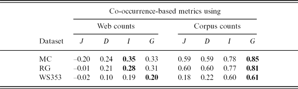
We consider as baseline the performance of the following metrics: (1) context-based similarity metric QH, defined in Section 3.2, (2) co-occurrence-based metrics, defined in Section 3.1, relying on counts that were computed either using the web as a corpus (number of hits), or the corpus of snippets harvested with respect to the 8, 752 nouns (Corpus4). The baseline scores for the context-based similarity metric QH are presented in Table 1, for several values of the contextual window size H. The best correlation scores are obtained for H = 1 across all datasets, while the performance drops as the size of the contextual window increases. Even for H = 1, moderate correlation scores are achieved for the MC and RG datasets, while the baseline performance is poor for the WS353 dataset. These results indicate the inability of naive context-based similarity metrics to exploit contextual features despite the availability of a large corpus. The baseline performance for co-occurrence-based metrics that incorporate web countsFootnote 9 (hits) or corpus counts (Corpus4) is shown in Table 2. Regarding corpus counts, the co-occurrence of nouns is considered at the snippet boundary. We observe that the employment of corpus counts leads to significantly higher correlation scores, compared to using web counts. For example, the correlation improves from 0.33 to 0.85 using the G metric for the case of the MC dataset. This observation is consistent for all metrics across all three datasets. For corpus counts, the best performance is achieved by the Google-based Semantic Relatedness, G, while the Mutual information, I, is a close second. Jaccard, J, and Dice, D, coefficients have lower but comparable performances.
Performance of context-based metric QH for several values of H

Performance of co-occurrence-based metrics using web and corpus counts: Jaccard (J), Dice (D), Mutual info. (I), and Google-based sem. rel. (G)
Despite the high performance of co-occurrence metrics using corpus counts, their applicability is strongly depended on the corpus size. The percentage of highly related noun pairs that have zero co-occurrence (corpus) counts are presented in Table 3 for several numbers of downloaded snippets. We assumed that two nouns are highly related if the corresponding similarity score (normalized between 0 and 1) provided by human subjects is greater than 0.5. The reported number of snippets is randomly selected from the initial (full) corpus. We observe that for the RG and WS353 datasets, even for the maximum number of snippets (1,000 per noun) 3–5percent of the highly related pairs do not co-occur.
Percentage of highly related pairs that have zero co-occurrence corpus counts as a function of downloaded snippets

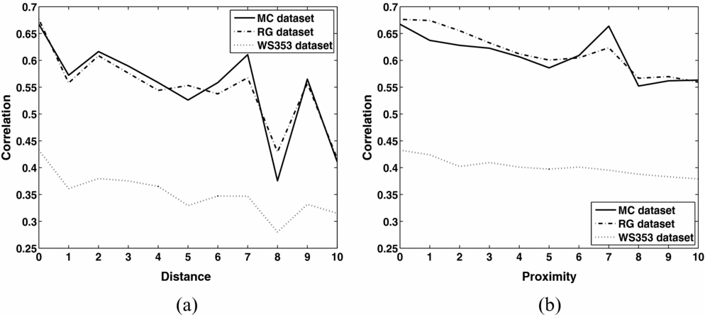
The poor performance of co-occurrence-based metrics that rely on web counts may be attributed to the fact that the co-occurrence of words is estimated at the document level, rather than at the level of snippet or sentence (for corpus counts). The key difference between web and corpus counts is the proximity of the co-occurring words as well as the different corpus statistics shown in Figure 1. In order to investigate the role of proximity, we formulated NEAR queries that constrain the distance between two words in an AND web query.Footnote 10 The performance of the I metric using web counts is presented as a function of the distance and proximity of co-occurring words (within documents) in Figures 3(a) and 3(b), respectively. The distance, δ, between two co-occurring words denotes that exactly δ tokens interfere between them. The proximity, πδ, of two words allows π tokens to appear between them, where 0 ⩽ πδ ⩽ δ. We observe that imposing a distance/proximity constraint significantly improves the achieved correlation compared to the baseline of web co-occurrence counts in Table 2. For example, the correlation for the RG dataset improves from 0.28 (see Table 2) to 0.68 for δ = 0 and π0. Despite the clear improvement in the performance of web-based count performance (when applying a proximity constraint), corpus-based counts still outperform web-based counts. The second reason behind the superior performance of corpus-based counts is the (normalized) word frequency statisticsFootnote 11 of the snippet corpus (versus web) shown in Figure 1.
Correlation performance of the co-occurrence-based metric I versus word (a) distance and (b) proximity (within web documents).
7.2 Incorporating word senses through web queries
We compare the performance of context-based similarity metrics for web corpora created via AND or IND queries. All results reported in this section are for the MC dataset. Baseline similarity scores here are computed using the Q H = 1 metricFootnote 12 defined in (6).
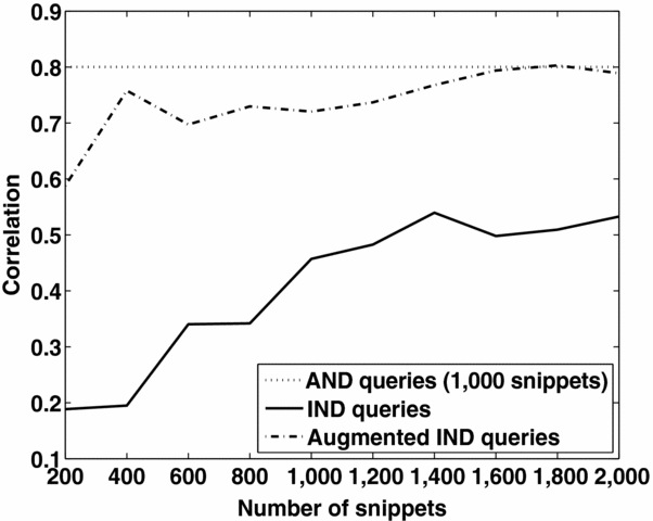
The correlation scores for the context-based similarity metric using AND and IND queries (dotted and solid lines, respectively) are shown in Figure 4 as a function of the number of snippets. The performance for AND queries is a single point and was obtained at 1,000 queriesFootnote 13 (shown here as reference). It is clear that context-based similarity metrics perform much better when using AND rather than IND queries.
Correlation performance for context-based similarity for web corpora created via AND queries (dotted), IND queries (solid), and IND queries augmented with sense descriptors (dashed-dotted) for the MC dataset.
Our hypothesis is that the very good performance of AND queries is due to co-occurrence acting as a semantic filter that retains the two closest senses of the two words. Moreover, the poor performance of IND queries is due to the limited coverage of senses within the top snippets. In order to verify this hypothesis, we perform (sense) filtering explicitly following three steps: (1) identify all senses of the words of interest using WordNet,Footnote 14 (2) use conjunctive AND queries between a word and each of its word senses to obtain relevant snippets that (mainly) contain the desired sense, e.g. the IND query for ‘magician’ becomes ‘magician AND illusionist’ (augmented), given the first WordNet sense of this word, and (3) compute the context-based similarity between all possible pairs of word senses and select the maximum similarity. Step 3 makes the implicit assumption that word similarity should be computed between the two closest senses (Budanitsky and Hirst Reference Budanitsky and Hirst2006), i.e. if sik is the kth sense of the word wi, the maximum sense context-based similarity Q′ between words wi, wj is defined as
 \begin{equation}
Q^{\prime }(w_i,w_j) = \max _{k,l} Q(s_{ik}, s_{jl})
\end{equation}
where Q is defined in (6). The performance of the augmented IND queries is shown in Figure 4 with a dashed–dotted line. It is clear that the use of the augmented IND queries significantly outperforms simple IND queries and approaches the performance of AND queries with increase in the number of snippets.
Overall, the presented results suggest that the exploitation of word senses is essential for the accurate computation of semantic similarity. We have also experimentally demonstrated that context-based semantic similarity estimates are more accurate if we consider the two closest senses, i.e. the maximum pairwise sense similarity score. A major road-block in top-down corpus creation using IND queries is the lack of sense coverage in the corpus. We show next that by creating a corpus by posing IND queries for thousands of words as well as by employing the notion of semantic neighborhood we can overcome this roadblock and obtain excellent semantic similarity estimates.
7.3 Semantic network
Next, we investigate the computation of semantic networks using different types of similarity metrics. Next, we present the evaluation results for the proposed neighborhood-based similarity metrics, defined by (8)–(10), for different ways of defining the semantic neighborhoods.
7.3.1 Semantic neighborhoods
The semantic neighborhood of each word is estimated using one of the co-occurrence-based metrics defined in Section 3.1, or the context-based similarity metric QH defined in Section 3.2. Our semantic network consists of 8, 752 nouns.
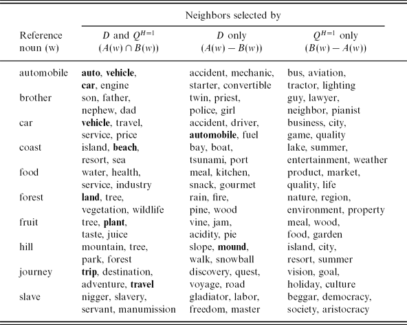
Given a (reference) noun w, let A(w) and B(w) be the neighborhood sets of w computed using co-occurrence- and context-based metrics. The intersection of A(w) and B(w), A(w)∩B(w) as well as their differences, A(w) − B(w) and B(w) − A(w), are shown in Table 4 for ten nouns that are included in the experimental datasets. The co-occurrence-based metric D defined in (2) was applied for the computation of A(w), while the context-based metric Q H = 1 defined in (6) was used for the computation of B(w). For both metrics, the fifty top-ranked neighbors were considered. The neighbors that are emphasized using bold fonts denote (lexicalized) senses of the respective reference nouns.
Excerpts of semantic neighborhoods for ten nouns using the co-occurrence- based metric Dice (D) and/or the context-based metric Q H = 1
We observe that the discovery of a number of senses via the neighborhoods is feasible for some nouns, e.g. ‘automobile’ and ‘car’. This is more clear for A(w)∩B(w) compared to A(w) − B(w) and B(w) − A(w). However, sense discovery appears to be difficult for other nouns, such as ‘food’ and ‘slave’, for which their respective senses cannot be easily described by single words. In addition to synonymy, taxonomic relations are encoded by the neighbors of A(w)∩B(w), e.g. IsA(vehicle, car), PartOf(automobile, engine). Relations of associative nature, e.g. ProducedBy(industry, food), are also denoted by some neighbors of A(w)∩B(w). Essentially, the main difference between A(w) − B(w) and B(w) − A(w) is that the former includes members that tend to formulate more direct associative relations with the reference nouns. In some cases these relations appear in the corpus as bigrams, such as ‘car accident’ and ‘hill slope’. Members of B(w) − A(w) seem to correspond to relations of a broader semantic/pragmatic scope, such as (food, life) and (journey, culture).
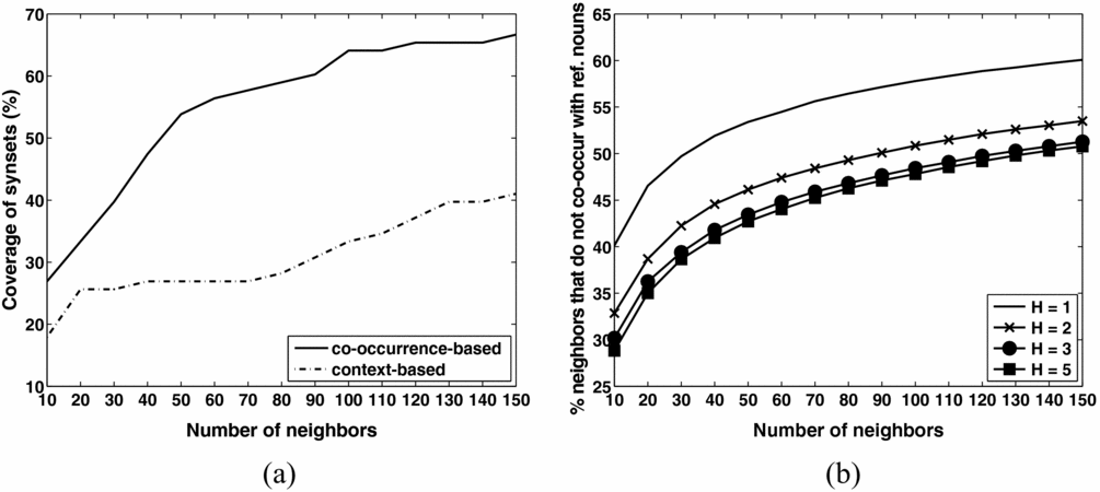
Given the importance of senses for the computation of semantic similarity, we attempt to quantify the performance of co-occurrence and context-based metrics with respect to the discovery of senses through their neighborhoods. The percentage of synonyms of reference nouns (taken from the RG dataset) that are included in the neighborhoods are presented in Figure 5(a) as a function of the neighborhood size. The sets of synonyms for each reference noun were created by consulting the WordNet synsets. The semantic neighborhoods were computed using either the co-occurrence metric D, or the context metric Q H = 1. In general, more synonyms are captured by the D metric compared to the Q H = 1 metric. This distinction is greater for neighborhoods that include more than fifty members.
(a) Percentage of WordNet synonyms included in the semantic neighborhoods versus number of neighbors. The neighborhoods were computed using 1) co-occurrence-based metric D (solid line), and 2) context-based metric Q H = 1 (dash–dotted line). The reference nouns were taken from the RG dataset. (b) Percentage of neighbors that do not co-occur with the reference nouns versus number of neighbors. In total, 1, 000 reference nouns were randomly selected from the lexicon. The neighborhoods were computed by the context-based metric QH. The percentage is shown for different values of H.
Moreover, we investigate the effect of the context window H with respect to the selection of neighbors that do not co-occur with the reference nouns. The percentage of such neighbors computed by QH is depicted in Figure 5(b) for several sizes of the neighborhoods, and for four values of the contextual window size H. The percentages were computed for 1, 000 nouns that were randomly selected from the network. The best results are consistently obtained when using immediate context, i.e. H = 1, which can be attributed to the best performance of this window value for the case of context-based similarity computation (Iosif and Potamianos Reference Iosif and Potamianos2010). This is also shown in Table 1.
7.3.2 Neighborhood-based metrics
The computation of semantic similarity consists of two basic steps:
(1) computation of semantic neighborhoods, and (2) computation of similarity scores (the S metric in (8) and (9)), allowing for the following combinations:
• Compute neighborhoods and similarity scores using a co-occurrence-based metric (CC/CC).
• Compute neighborhoods using a co-occurrence-based metric; compute similarity scores using a context-based metric (CC/CT).
• Compute neighborhoods using a context-based metric; compute similarity scores using a co-occurrence-based metric (CT/CC).
• Compute neighborhoods and similarity scores using a context-based metric (CT/CT).
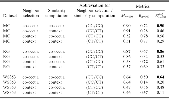
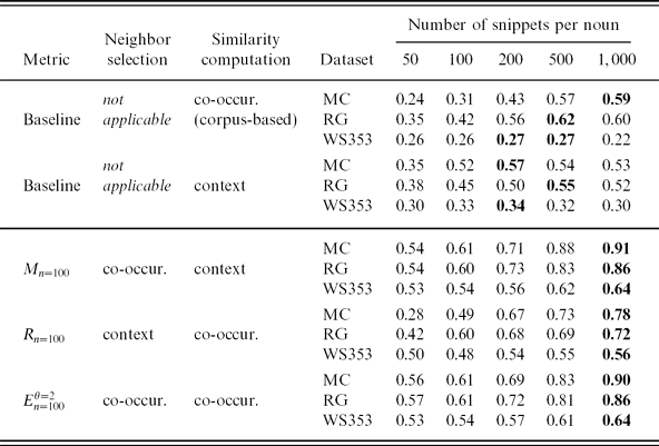
For the above approaches, the co-occurrence-based metricFootnote 15D and the context-based metric Q H = 1 were used. The correlation results for the neighborhood-based metrics M n = 100, R n = 100, and E θ = 2n = 100 for neighborhood size of one hundred are presented in Table 5 (see the next paragraph for the choice of n). The use of a co-occurrence metric for neighbor selection achieves the highest results for all datasets, M n = 100 and E θ = 2n = 100, while the context-based metric appears to be better for selecting neighbors for the correlation-based neighborhood metric R n = 100. The choice of the semantic similarity metric is of secondary importance for the M n = 100 and R n = 100 metrics, provided that the appropriate metric is used for neighborhood creation. For the E θ = 2n = 100 metric, however, only the (CC/CC) combination performs well. The results are significantly higher compared to the context-based baselines (see Table 1). The best M n = 100 and E n = 100 metrics also outperform the metrics that rely on web or corpus counts. Overall, utilizing network neighborhoods for estimating semantic similarity can achieve very good performance, and the type of metric (feature) used to select the neighborhood is a key performance factor.
Correlation for neighborhood-based metrics. Four combinations of the co- occurrence-based metric Dice (D) and the context-based metric Q H = 1 were used for the definition of semantic neighborhoods and the computation of similarity scores
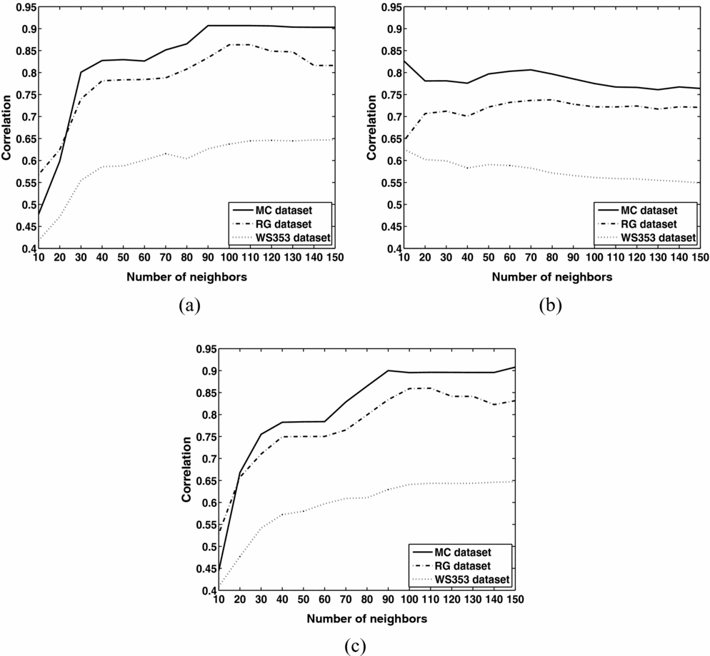
Next, we investigate the performance of the metrics as a function of neighborhood size n. The performance of the Mn metric using co-occurrence-based metric D for neighbor selection, and Q H = 1 for similarity computation is shown in Figure 6(a). We observe that performance increases with n peaking around, i.e. n = 80 − 100. The performance also remains high for n > 100. The performance of the Rn metric using Q H = 1 for neighbor selection and D for similarity computation is shown in Figure 6(b). The performance of Rn is relatively flat as a function of neighborhood size, achieving good performance even for small neighborhoods. The performance of the E θn metric using D for both neighborhood selection and similarity estimation is shown in Figure 6(c). Mn and E θn exhibit comparable performances, while both appear to be better than Rn for high values of n.
Performance versus number of neighbors for neighborhood-based metrics: (a) maxi- mum similarity of neighborhoods Mn: (CC/CT), (b) correlation of neighborhood similarities Rn: (CT/CC), and (c) sum of squared neighborhood similarities E θn: (CC/CC).
The correlation scores for the best performing neighborhood metrics (M n = 100, R n = 100, and E θ = 2n = 100 for the (CC/CT), (CT/CC), and (CC/CC) approaches, respectively) are presented in Table 6 as a function of the number of snippets downloaded for each word in the network. The performance of the corresponding baseline metrics are also shown in Table 6, i.e. the D metric relying on corpus counts, and Q H = 1. We observe that the neighborhood metrics outperform the baseline performance for all datasets. All three neighborhood metrics consistently obtain better correlation performance with increase in the number of snippets. Unlike neighborhood metrics, the performance of baseline metrics is not shown to improve as the number of snippets increases and plateaus around 300–500 snippets.
Performance with respect to the number of corpus snippets per noun for the baseline and the neighborhood-based metrics
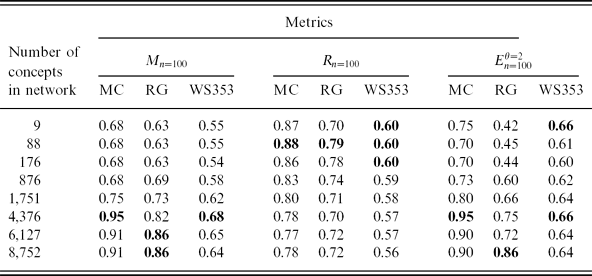
Next, we investigate the performance of the neighborhood metrics with respect to the number of concepts (nouns) included in the network. The concepts were randomly selected; results are presented in Table 7 in the form of average correlation computed over ten runs. We experimented with various network sizes varying from nine (0.1 percent of the network) up to 8, 752 (100 percent of the network) words. Regarding the M n = 100 and E θ = 2n = 100 metrics, performance improves as the network grows with best results around 4,000–5,000 words. Conversely, R n = 100 performs best for small networks.Footnote 16
Performance of neighborhood metrics for various network sizes
7.4 Fusion of neighborhood metrics
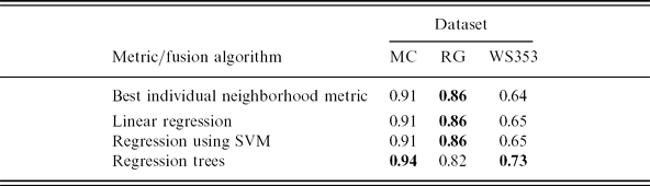
Next, we investigate the fusion of the best performing neighborhood metrics, Mn, Rn, and E θ = 2n, using the (CC/CT), (CT/CC), and (CC/CC) combinations, respectively (see Table 5). The fusion was performed as a weighted linear combination of their respective similarity scores. The largest dataset, i.e. WS353, was used for learning the weights of similarities using ten-fold cross-validation. Then the weights learned on (all of) WS353 were applied to the CM and RG datasets. Three different algorithms implemented in WekaFootnote 17 were applied for learning the weights, namely linear regression, regression using Support Vector Machines (SVM), and regression trees. The performance of the fusion of metrics is presented in Table 8 for n = 100, along with the performance of the best individual neighborhood metric.Footnote 18
Performance for the fusion of neighborhood metrics
We observe that the performance of fusion using linear and SVM-based regression is almost identical to the performance of the best individual neighborhood metric. Performance gains are obtained using regression trees for the CM (from 0.91 to 0.94) and WS353 datasets (from 0.64 to 0.73). However, performance is worse on the RG dataset. This trend is probably due to the different distribution of similarity scores in the datasets (MC dataset, for example, contains only highly similar or dissimilar word pairs, while RG contains more uniformly distributed similarity scores).
7.5 Comparison with other approaches
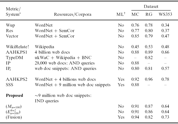
A comparison between our best resultsFootnote 19 and the performance of other similarity metrics is summarized in Table 9. The primary criterion for the selection of the presented metrics is the type of the exploited resources and corpora. This enables the comparison between knowledge- and data-driven approaches, while the latter often are the only feasible choice for under-resourced languages. The approaches that are presented in Table 9 can be distinguished into two main categories: (i) Use of knowledge resources, such as WordNet, and (ii) use of large corpora, e.g. Wikipedia and corpora harvested from the web. In addition, we consider a third category dealing with the integration of (i) and (ii) within a machine learning-based framework.
Performance of several metrics/systems
* The metrics/systems shown in full uppercase, e.g. IP, were abbreviated using the first letter of authors’ last names.
† Use of machine learning.
Three basic types of WordNet-based metrics are included in category (i): path length-based (Wup), information content-based (Res), and metrics that exploit the synset glosses (Vector). Wup (Wu and Palmer Reference Wu and Palmer1994) is a purely taxonomic metric based on the notion of the least common subsumer (LCS), i.e. the most specific concept that is the parent node of two words. The similarity between two words, wi and wj, is estimated as the depth (distance from root node) of their LCS, normalized by their individual depths (Pedersen Reference Pedersen2010). Wup is extended by the Res metric (Resnik Reference Resnik1995), according to which the similarity between wi and wj is estimated as Res(wi, wj) = −log P(LCS(wi, wj)), where P(LCS(wi, wj)) is the probability of the LCS of wi and wj estimated over a sense-tagged corpus (Pedersen Reference Pedersen2010). The lexical information that is included in the WordNet glosses is utilized by the Vector metric (Patwardhan and Pedersen Reference Patwardhan and Pedersen2006) for the construction of co-occurrence vectors extracted from a sense-tagged corpus. The similarity between wi and wj is estimated as the similarity between their respective vectors. In this work, we applied the aforementioned WordNet-based metrics using the WordNet::Similarity module,Footnote 20 which incorporates the SemCor corpus (Pedersen and Michelizzi Reference Pedersen and Michelizzi2004). More specifically, the similarity between two words was estimated according to (11) following the maximum sense similarity assumption (Resnik Reference Resnik1995; Budanitsky and Hirst Reference Budanitsky and Hirst2006). Regarding category (ii), the WikiRelate! system (Strube and Ponzetto Reference Strube and Ponzetto2006) includes various taxonomy-based metrics that are typically applied to the WordNet hierarchy. The basic idea behind WikiRelate! is to adapt these metrics to a hierarchy extracted from the links between the pages of the English Wikipedia. A very large corpus is exploited by AAHKPS1 consisting of four billion web documents that were acquired via crawling (Agirre et al. Reference Agirre, Alfonseca, Hall, Kravalova, Pasca and Soroa2009). For the computation of semantic similarity, several variations of structured and unstructured DSM were applied. An example of structured DSM is the TypeDM model (Baroni and Lenci Reference Baroni and Lenci2010), where a number of lexico-syntactic patterns were extracted from the concatenation of three different corpora, namely the web-harvested ukWaC corpus,Footnote 21 the dump of the English Wikipedia, and the British National Corpus (BNC). Our previous work, IP, is an example of corpus creation using a relatively small number of web documents (Iosif and Potamianos Reference Iosif and Potamianos2010). The basic idea was the use of conjunctive AND queries to retrieve documents in which the pair words co-occur. Also, we have replicatedFootnote 22 our previous work using snippets instead of entire web documents (IPs).
The third category that appears in Table 9 includes the following machine learning-based metrics/systems: AAHKPS2 and SSS. The basic approach behind AAHKPS2 (Agirre et al. Reference Agirre, Alfonseca, Hall, Kravalova, Pasca and Soroa2009) is the use of regression to combine similarity scores that were computed using different resources and corpora. A corpus of four billion web documents was exploited and results were derived using ten-fold cross-validation. A different approach was followed by the SSS system (Spanakis, Siolas and Stafylopatis Reference Spanakis, Siolas and Stafylopatis2009) according to which the WordNet was exploited to create thousands of word pairs denoting relations such as synonymy, meronymy, etc. These pairs were used for the formulation of web queries to create a corpus of snippets from which numerous lexico-syntactic patterns were extracted. The word similarity was estimated by a regression model considering the pattern frequencies as training features. The WS353 dataset was used for training excluding the pairs of the MC dataset, which were used for testing.
As it was expected, the exploitation of knowledge resources leads to high performance. The superiority of the Vector metric over other WordNet-based metrics constitutes a successful paradigm regarding the exploitation of contextual features given that the word senses are knwon. The performance of the DSM-based approaches, i.e. AAHKPS1, TypeDM, and IP, is higher compared to the WordNet metrics. This observation is more interesting regarding the case of IP, where a relatively small corpus of web documents is used. The proposed metrics clearly outperform the resourced-based approaches: WordNet-based (Wup, Res, Vector) and Wikipedia-based (WikiRelate!), and also obtain higher results than the paradigm of structured DSM (TypeDM). Also, the utilization of IND queries yields better performance compared to our previous work using AND queries (IP, IPs). Regarding unsupervised approaches (i.e. no use of machine learning), AAHKPS1 appears to be the closest competitor to the proposed metrics. Overall, the best performance is obtained by the machine learning-based approaches AAHKPS2 for the RG and WS353 datasets, and the fusion of M n = 100, R n = 100, and E θ = 2n = 100 for the MC dataset. However, we believe that further validation is needed for the machine learning approaches given the limited size of the datasets and the dangers of overfitting. Overall, the proposed M n = 100 and E θ = 2n = 100 metrics can be regarded among the best-performing unsupervised data-driven metrics, built upon an efficient and scalable approach for corpus creation using web data.
8 Conclusions
We have investigated the estimation of semantic similarity using semantic networks, following an unsupervised corpus-based approach. We have shown that it is possible to achieve state-of-the-art performance by encoding corpus statistics into a semantic network and then using the notion of semantic neighborhood to define novel semantic similarity metrics. The maximum neighborhood similarity metric performed the best when the semantic neighborhood was defined using co-occurrence metrics. We have also shown experimentally the importance of sense coverage and the validity of the maximum sense similarity assumption for context-based similarity metrics.
The fact that co-occurrence proved to be a good feature for selecting neighbors for the maximum similarity metric implies that co-occurrence is a good feature for sense discovery. Moreover, we have studied the effect of word proximity for the estimation of semantic similarity, showing that very good performance is obtained when words co-occur at sentential level. The success of context-based similarity for neighborhood selection for the correlation metric implies that context is a good feature for discovering attributes in a network. In addition, the use of a corpus in which the not so common words are well represented and a large lexicon creates an informative corpus that efficiently encodes the semantics of polysemous words and leads to good performance. More research and experimentation is needed to verify these claims. Overall, the achieved results are among the highest reported in the literature for unsupervised corpus-based metrics. Last but not least, the proposed approach is efficient, scalable, and requires linear web query complexity with respect to the lexicon size.
A series of preliminary experiments were conducted to investigate the applicability of the proposed approach to other semantic tasks, namely compositional similarity estimation for noun–noun compounds, and word semantic similarity using networks of words and images. Very encouraging results were obtained for both tasks, which show the extensibility of network-based DSM to compositional and multimodal semantic similarity tasks. Future work deals with the incorporation of network features, such as centrality measurements, for the creation of semantic neighborhoods. Further research is needed with larger multilingual networks to verify the universality of the proposed metrics.
Acknowledgments
This work has been been partially funded by the PortDial project (‘Language Resources for Portable Multilingual Spoken Dialog Systems’) supported by the EU Seventh Framework Programme (FP7), grant number 296170. Also, Elias Iosif was partially funded by the Basic Research Programme, Technical University of Crete, Project Number 99637: ‘Unsupervised Semantic Relationship Acquisition by Humans and Machines: Application to Automatic Ontology Creation’. The authors wish to thank Nikos Malandrakis for many useful discussions and applying neighborhood-based similarity metrics to affective text computation.