
 Larλ





1. Background
1.1 On type-theory of recursion and algorithms
By Moschovakis (Reference Moschovakis1989, Reference Moschovakis, Oikkonen and Väänänen1993, Reference Moschovakis, Dalla Chiara, Doets, Mundici and van Benthem1997), Yiannis N. Moschovakis introduced the untyped version of the mathematical notion of algorithm via the formal language of recursion (FLR). The theory of FLR provides denotational and algorithmic semantics of its untyped formal language. The denotational semantics of FLR covers the mathematical structures having as their domain spaces the sets of functions determined by full recursion. Significantly, the algorithmic semantics of the FLR provides algorithms for computing the denotational values of the algorithmically meaningful FLR terms, in the space of recursive functions. The algorithmically meaningful FLR terms of full recursion designate algorithms that may be cyclic without ending.
The type-theory of acyclic recursion (TTAR)
 $\operatorname {L^{\lambda }_{ar}}$
, that is, of acyclic algorithms, was introduced by Moschovakis (Reference Moschovakis2006). In distinction to the untyped FLR, which includes endless cyclic algorithms, the type-theory
 $\operatorname {L^{\lambda }_{ar}}$
formalizes algorithms that terminate, that is, close-off, after finite number of steps of calculations. In Moschovakis (Reference Moschovakis2006), the focus is on demonstrating potential applications of
 $\operatorname {L^{\lambda }_{ar}}$
to computational semantics of natural language (NL), by an approach that is similar to semantics of programming languages. The language of
 $\operatorname {L^{\lambda }_{ar}}$
limits the set of its
 $\operatorname {L^{\lambda }_{ar}}$
terms by an acyclicity criterion given in Definition 3 of this article.
For an initial introductions to type-theory
 $\operatorname {L^{\lambda }_{ar}}$
of recursion, its syntax, its distinctive two kinds of semantics, namely denotational and algorithmic semantics, and reduction calculus, see Moschovakis (Reference Moschovakis2006). Formally, the
 $\operatorname {L^{\lambda }_{ar}}$
terms in Moschovakis (Reference Moschovakis2006) are defined by the clauses of the form (3a)–(3d) given in Definition 2 of this article, which satisfy the Acyclicity Constraint (AC) in Definition 3.
For detailed, formal introduction to the syntax and extended reduction calculus of TTAR
 $\operatorname {L^{\lambda }_{ar}}$
, its denotational and algorithmic semantics, see Loukanova (Reference Loukanova2019b). Further developments of TTAR
 $\operatorname {L^{\lambda }_{ar}}$
consist of extended formal languages and computational facilities of
 $\operatorname {L^{\lambda }_{ar}}$
, see Loukanova (Reference Loukanova, van den Herik and Filipe2016a, Reference Loukanova2016b, Reference Loukanova, Osswald, Retoré and Sutton2019a, Reference Loukanova2019b, Reference Loukanova, Grabowski, Loukanova and Schwarzweller2020, Reference Loukanova, Materna and Jespersen2022, Reference Loukanova2023b, Reference Loukanova2023c, Reference Loukanova2023d, Reference Loukanova, Bekki, Mineshima and McCready2024).
Often, I use the same designation of the developed classes of TTAR and algorithms, that is, TTAR, TTAA, or
 $\operatorname {L^{\lambda }_{ar}}$
. These classes suffice for representing significant fragments of NL.
1.2 Other systems for formal semantics of NLs
In this section, I present some of the formal systems for semantic representations of NL expressions, which have some significance with respect to
 $\operatorname {L^{\lambda }_{ar}}$
.
Originally, Russell (Reference Russell1905) proposed a logic system without types, for semantic representations of NL sentences consisting of combinations of verbs (Vs) and noun phrases (NPs). In the Russel logic, the semantic denotation of a sentence, which is a combination of an NP and a VP expressions, is the result of application of the function, which denotes the NP expression, to the denotation of the VP expression.
The papers Henkin (Reference Henkin1950) and Mostowski (Reference Mostowski1957) formalized Russel’s proposal by higher-order logic. Importantly, Mostowski (Reference Mostowski1957) introduced the logic of generalized quantifiers, which are essential for semantics of quantified expressions.
In several papers, Richard Montague extended the ideas of generalized quantifiers to the comprehensive formal semantics of a fragment of NL. Most successfully, Montague (Reference Montague, Hintikka, Moravcsik and Suppes1973) introduced Intensional Logic (IL) for semantic representation of NL quantifiers and intensional verbs, in his system of The Proper Treatment of Quantification (PTQ). His IL uses higher-order, simply typed, lambda calculus. In Montague IL, all NPs, including proper names, are translated into one-argument generalized quantifiers. All verbs, extensional and intensional, which have syntactic arguments requiring NPs, are translated into terms of “shifted up” types for suitable combinations with the types of the generalized quantifiers. The essential translation system into IL terms uses
 $\beta$
-conversions and meaning postulates to transform and simplify the resulting IL terms to typical logic terms. Following Montague IL and PTQ, various systems of formal semantics of NL fragments have been proposed in similar styles.
The concepts of the generalized quantifiers continue to be an essential type-theoretical facility, especially for formal semantics of NL, including in the algorithmic semantics of
 $\operatorname {L^{\lambda }_{ar}}$
.
The type-theory
 $\mathrm{TY}_2$
introduced by Gallin (Reference Gallin1975) is a significant move towards representation of context by states into the formal language and semantics of
 $\mathrm{TY}_2$
, which is a basis for generalizations of type-theoretic semantics of NL. A major result of Gallin (Reference Gallin1975) is the interpretation of Montague IL, which was introduced by Montague (Reference Montague, Hintikka, Moravcsik and Suppes1973) and Thomason (Reference Thomason1974), in
 $\mathrm{TY}_2$
.
Muskens l
ambda t
ype-
t
heory. Muskens relational logic
 $\textit{TT}_2$
, Muskens (Reference Muskens1995), is the basis for type-theoretic semantics in the Muskens generalized grammar (MGGr) that he developed. It covers partiality of semantic relations and generalized quantifiers. For introductions to MGGr, by comparing
 $\mathrm{TY}_2$
with IL, see Muskens (Reference Muskens1995) and Loukanova (Reference Loukanova, Bekki, Mineshima and McCready2023e).
Sadrzadeh and Muskens (Reference Sadrzadeh and Muskens2019) is a development of Muskens type-logic grammar. In the dynamic models of lambda calculus, the degree of co-occurrence of words in context determines similarity of words’ interpretations in the correspondingly changed context. Interesting questions emerge regarding whether and, if yes, how the type-theory
 $\operatorname {L^{\lambda }_{ar}}$
can be integrated with dynamic vector models for lambda calculus, towards further generalizations of algorithmic semantics of NL.
Type-
t
heory of a
cyclic r
ecursion in r
elation to G
allin t
ype-
t
heory. The formal language of
 $\operatorname {L^{\lambda }_{ar}}$
strictly extends (Gallin Reference Gallin1975) type-theory
 $\mathrm{TY}_2$
, and by that (Montague Reference Montague, Hintikka, Moravcsik and Suppes1973) IL. Loukanova (Reference Loukanova2023c), Sections 4 and 5, gives a mathematical proof of this expressiveness of an extended version of
 $\operatorname {L^{\lambda }_{ar}}$
. TTAR,
 $\operatorname {L^{\lambda }_{ar}}$
, has recursion terms that are not algorithmically equivalent to any
 $\lambda$
-calculus, for example,
 $\mathrm{TY}_2$
terms. Such
 $\operatorname {L^{\lambda }_{ar}}$
recursion terms provide subtle semantic distinctions via computational algorithms of
 $\operatorname {L^{\lambda }_{ar}}$
.
Similarly to
 $\mathrm{TY}_2$
,
 $\operatorname {L^{\lambda }_{ar}}$
has the following characteristics:
Currying.
 $\operatorname {L^{\lambda }_{ar}}$
uses currying encoding of multi-argument relations and functions via one-argument functions, which is the basis of techniques often used in functional programming and other formal languages.
States and state dependency.
 $\operatorname {L^{\lambda }_{ar}}$
has types and terms designating states and state-dependent objects. In general, the nature of the states in the semantic domains of
 $\operatorname {L^{\lambda }_{ar}}$
can be left open and introduced depending on applications of
 $\operatorname {L^{\lambda }_{ar}}$
. Moschovakis (Reference Moschovakis2006) tentatively presented states as ordered tuples of components that represent context information for semantic denotations of NL expressions. Detailed context elements are formally used as situations, agents, space, and time locations in Situation Theory and Situation Semantics, see Loukanova (Reference Loukanova, Nguyen, Kowalczyk, Fred and Joaquim2014, Reference Loukanova2023a).
Passives in HPSG approach. Syntax–semantics analysis of the passives was introduced since the early stages of HPSG, see Pollard and Sag (Reference Pollard and Sag1994) and Sag et al. (Reference Sag, Wasow and Bender2003). Their approach reflects on solid linguistic research and significance of linguistic generalizations across syntactic structures of NL. My work on the syntax–semantics interfaces in NL is inspired and based on such significance of linguistic generalizations. The formal representation of the lexical and phrasal syntax of the passives, via feature-structure descriptions, which I employ for the syntax of NL, is bassed on the corresponding rules in Sag et al. (Reference Sag, Wasow and Bender2003).
1.3 On computational grammar of NL
A detailed introduction to a class of approaches of formal grammar of NL called Constraint-Based Lexicalized Grammar (CBLG), with linguistic motivations and bibliography, is given in Sag et al. (Reference Sag, Wasow and Bender2003). A formal generalization of the CBLG approaches covered in Sag et al. (Reference Sag, Wasow and Bender2003) is presented in Loukanova (Reference Loukanova2017), which, sometimes, I call generalized CBLG (GCBLG), by a focus on its mathematical models of linguistic information in functional domains. While GCBLG appears closest to the approach of Head-Driven Phrase Structure Grammar (HPSG), it covers common linguistic trends in varieties of other approaches to formal and computational syntax. In particular, in what follows, I list a related, major classification of approaches to formal grammar of NL, which includes many other specific classes of formalizations:
-
Phrase Structure Grammars and Transformational Grammars: 1955–64; for example, see the initiation towards computational syntax (Chomsky Reference Chomsky1957, Reference Chomsky1965).
-
Generalized Phrase Structure Grammar (GPSG): 1979–87; for example, see the beginnings of actual computational syntax by Gazdar et al. (Reference Gazdar, Klein, Pullum and Sag1985).
-
Lexical Functional Grammar (LFG): 1979 to the present; for example, see Bresnan (Reference Bresnan2001) and Dalrymple (Reference Dalrymple2001, Reference Dalrymple2023)
-
Head-driven Phrase Structure Grammar (HPSG): since Pollard and Sag (Reference Pollard and Sag1994) and Müller et al. (Reference Müller, Abeillé, Borsley and Koenig2024) to the present, a linguistic approach and large-scale computational grammar of NL, see DELPH-INS (2025).
-
Constraint-Based L exicalized Grammar (CBLG): approaches to formal and computational syntax of NL, which represents comprehensive, linguistically motivated syntactic structures. Sag et al. (Reference Sag, Wasow and Bender2003) is a detailed introduction to the approaches of formal grammar of NL, giving references by extensive descriptions. The authors motivate the development of CBLG family of approaches to formal grammar of NL, starting with Finite State Automata and Context Free languages. Loukanova (Reference Loukanova2017) presents a possibility for mathematical models of syntactic structures of a class of formal languages of CBLG. The syntactic descriptions in CBLG are modeled by mathematical structures of sets of functions that represent complex, linguistically motivated information. The functions are recursively defined over linguistic features and take as values also such functions, which can be atomic or complex.
-
Categorial Grammar (CG): 1970 to the present. CG was originally developed by Ajdukiewicz (Reference Ajdukiewicz1937) as a mathematical theory suitable for significant syntactic structures of NL. See Carpenter (Reference Carpenter1998) for an extensive introduction and overview of the CG approaches.
-
Grammatical Framework (GF): GF is a type-theoretical formalism, with highly promising development for parallel, multilingual translation and text generation, see Ranta (Reference Ranta1994).
Computational syntax of NL has been well developed, in particular for widely used langages, for example, English, German, Norwegian, Japanese, etc. On the other hand, computational semantics and computational syntax–semantics interfaces, in computational grammar of NL, including CBLGs, are largely open research subjects.
1.4 Semantic representations in CBLG
Copestake et al. (Reference Copestake, Flickinger, Pollard and Sag2005) introduced the technique, called Minimal Recursion Semantics (MRS) and the formal language of MRS, in a semi-formal mode, while describing them strictly and clearly. Thus, MRS is a technique for formal representations of semantic information by specialized expressions of the language of MRS.
To some extent, MRS has been used in LFG, see Flickinger et al. (Reference Flickinger, Lønning, Dyvik, Oepen and Bond2005) on the initial implementation of the LOGON machine translation system.
HPSG is a well-developed, large-scale grammar, that is, HPSG approach, for various languages, especially for English, German, Norwegian, and Japanese, which also uses syntax–semantics interfaces via MRS, see DELPH-INS (2025).
Nowadays, MRS is well implemented and standardly used for semantic representation in HPSG approaches, see Müller et al. (Reference Müller, Abeillé, Borsley and Koenig2024), in particular Ch. 22 on MRS. The technique MRS in HPSG employs unification methods in varieties of the formal language of feature-value structure descriptions presented in Sag et al. (Reference Sag, Wasow and Bender2003). The syntax of HPSG is formalized by a more general GCBLG presented in Loukanova (Reference Loukanova2017).
Mathematical foundations of MRS in HPSG. The type-theory
 $\operatorname {L^{\lambda }_{ar}}$
presented in this paper provides a direct contribution to the mathematical foundation of the MRS technique implemented in the large-scale HPSG grammar approach. More precisely,
 $\operatorname {L^{\lambda }_{ar}}$
is mathematical foundation of MRS via currying encoding of semantic relations.
The mathematical model theory of situated, partial information, called Situation Theory, introduced and extended by Loukanova (Reference Loukanova, Nguyen, Kowalczyk, Fred and Joaquim2014, Reference Loukanova2023a), provides abstract mathematical objects that are recursively defined and depend on situations, times, space, and agents. The types, properties, and relations between objects are either primitive, that is, atomic, or complex and recursively defined, without currying encoding. Situation Theory has a special application to semantics of NL, called Situation Semantics.
In a specialized, restricted version, Situation Theory provides a mathematical foundation of the technique MRS, explicitly without currying encoding of properties and relations. Thus, MRS is an implementation technique for a version of Situation Semantics of NL.
One of the significant existing applications of
 $\operatorname {L^{\lambda }_{ar}}$
is the formalization of the semantic representations in the large-scale grammar approaches of HPSG, including by:
-
(1) initial representation of Situation Semantics expressions by the language of feature-value descriptions, and
-
(2) implementations of MRS in HPSG.
For an early development of TTAR and its application to mathematics of MRS, see Loukanova (Reference Loukanova, Bel-Enguix, Dahl and De La Puente2011b, Reference Loukanova, Bel-Enguix, Dahl and Jiménez-López2011a).
Note that semantic representations in HPSG, by MRS in feature-value descriptions, are representations of a simplified version of the specialized formal language of Situation Semantics presented in Loukanova (Reference Loukanova, Nguyen, Kowalczyk, Fred and Joaquim2014).
MRS uses constrained labels, that is, which are similar to specialized variables, where constraints are expressed by feature-value descriptions encoding formal terms of Situation Theory. The constrained MRS labels (variables) are formalized, via currying encoding, by restricted
 $\operatorname {L^{\lambda }_{ar}}$
terms, which are defined by the clauses of the form (3e) in Definition 2. A significant characteristic of MRS in HPSG, similarly to the syntax in HPSG, is that the facilities of lambda terms and calculus are not employed terms. That is efficiently compensated for by the HPSG hierarchy of typed constraints, suitably labeled by labels, which have the roles of variables and unification technique.
The formal language and mathematics of type-theory of TTAR,
 $\operatorname {L^{\lambda }_{ar}}$
, use the standard lambda terms for the compositional formation of terms and their denotational semantics, without reliance on unification methods. The algorithmic semantics of TTAR is provided by the specialized set of recursion variables, recursion terms, and reduction calculus; see the formal definitions and descriptions in Section 2.
My general contribution via TTAR,
 $\operatorname {L^{\lambda }_{ar}}$
, to Computational Grammar. Thus, the formal language and type-theory
 $\operatorname {L^{\lambda }_{ar}}$
provides the large-scale HPSG grammar including MRS expressions used in it, and the MRS technique presented independently outside HPSG grammar, with mathematical foundation and essential algorithmic semantics. My significant contribution (which is the first one up to my awareness) to MRS, HPS, and in general to Computational Grammar of NL is providing them with strict, reliable mathematical foundations, via developments of TTAR and the dependent-type-theory of situated information, that is, Situation Type-Theory of Situated Information and Semantics. TTAA,
 $\operatorname {L^{\lambda }_{ar}}$
, provides criterion for acyclicity in applications to computational syntax–semantics of NL.
I work on development of the mathematics of TTAR and utilizing TTAR for the semantic representations. In this paper, I incorporate the formal
 $\operatorname {L^{\lambda }_{ar}}$
terms inside feature-value structure descriptions of NL syntax. In addition, I often use standard context-free phrasal structure rules, including in this paper, for the syntax of NL to demonstrate how TTAR can be utilized for algorithmic syntax–semantics interfaces.
My contributions in this paper. I introduce the formal mathematics of TTAR. Then, I present the utility of TTAR for rendering NL passive forms, by descriptions and examples. TTAR has a rich language that allows optional terms for semantic representations of NL including passives. The selection depends on specific computational grammars and personal taste of a researcher. The canonical forms of TTAR terms provide criteria for algorithmic equivalence between terms. The mathematical characteristics of TTAR are among the many benefits of using TTAR for extending the existing approaches to computational semantics.
In addition, in this paper, I introduce a new way of rendering the passives, via specialized passivization marker, see the sections and examples on the verb “be” as a passivization marker. I add algorithmic patterns for representation of major classes of passives, by using such a marker, and without it.
A brief description of the content of the paper. In Section 2, I provide the formal syntax of type-theory
 $\operatorname {L^{\lambda }_{ar}}$
of acyclic recursion and algorithms (TTAR/TTAA). In Sections 3 and 4, I define the canonical forms and the extended reduction calculus of
 $\operatorname {L^{\lambda }_{ar}}$
. These computational concepts are valid also for the type-theory of full recursion and algorithms with cycles (TTR/TTA). Sections 5 and 6 introduce syntax–semantics interfaces via feature-structure descriptions. The rest of the paper introduces the application of TTAR to the syntax–semantics interfaces of passive forms in a generalized computational grammar, which includes connected lexical and phrasal structures.
In general, the algorithmic semantics of
 $\operatorname {L^{\lambda }_{ar}}$
presented in this paper can be employed for semantic representations of NL in a varieties of computational grammar, not only for CBLG approaches. In addition, I present a syntax–semantics technique via integration of semantic representations of NL, by the formal language of
 $\operatorname {L^{\lambda }_{ar}}$
, into CBLG syntax. In this paper, I focus on the specific linguistic phenomenon of passive forms of verbal expressions of NL.
In GCBLG, similar to Sag et al. (Reference Sag, Wasow and Bender2003) and Loukanova (Reference Loukanova, Bel-Enguix and Jiménez-López2011c), I use the typed version of the formal language of feature-value descriptions, also known as attribute-value matrices (AVMs), see Johnson (Reference Johnson1988). AVMs express linguistic information underlining syntactic structures of NL, by a combination of dependent types, which are organized hierarchically by constraints. Constraints and other linguistic information are expressed by formal features having corresponding values. This paper shows that GCBLG can be used for integration of syntax–semantics interface in it. The semantic representations in GCBLG do not necessarily use recourse to unification techniques. For the syntactic parts of the grammar analysis of NL, I use, as in Loukanova (Reference Loukanova, Bel-Enguix and Jiménez-López2011c), some of the major syntactic categories and structures, without detailed syntactic components.
2. Syntax of Type-Theory of Recursion and Algorithms
In this section, we define the classes of the formal languages of
 $\operatorname {L}^{\lambda }_{r}$
and
 $\operatorname {L^{\lambda }_{ar}}$
, as often in mathematical logic and computer science. By selecting literally fixed vocabulary, for example, constants, variables, connectors like
 $\lambda$
,
 $\land {}$
(
 $\And$
),
 $\lor {}$
,
 $\to {}$
, parentheses, comma, and (reasonably) small spaces, one can get concrete instances of the class of the languages of
 $\operatorname {L^{\lambda }_{ar}}$
(
 $\operatorname {L^{\lambda }_{r}}$
). In general, including in this paper, we assume a generic representative of the classes of the formal languages of
 $\operatorname {L^{\lambda }_{ar}}$
and
 $\operatorname {L}^{\lambda }_{r}$
, which is the object, formal language of
 $\operatorname {L^{\lambda }_{ar}}$
(
 $\operatorname {L^{\lambda }_{r}}$
), generally specific without being literally concrete.
Sometimes, we use letters or expressions, by assuming they are per se external, that is, not literally belonging to the formal language of
 $\operatorname {L^{\lambda }_{ar}}$
(
 $\operatorname {L^{\lambda }_{r}}$
). I use them as abbreviations designating term forms or specific terms. They can be useful when the designated terms are patterns or long. We may call them meta-symbols or meta-variables, in distinction of the variables belonging to
 $\operatorname {L^{\lambda }_{ar}}$
(
 $\operatorname {L^{\lambda }_{r}}$
). The expressions using such meta-variables designate terms of
 $\operatorname {L^{\lambda }_{ar}}$
(
 $\operatorname {L^{\lambda }_{r}}$
), if composed by the respective rules. For example, the symbols
 $\mathsf{e}$
,
 $\mathsf{s}$
, and
 $\mathsf{t}$
are the terminals, while
 $\tau$
,
 $\tau _1$
, and
 $\tau _2$
are auxiliary, non-terminals of a Context-Free Grammar.
In brief, meta-symbols and meta-variables are auxiliary symbols and expressions that are not strictly in the formal languages of
 $\operatorname {L^{\lambda }_{ar}}$
and
 $\operatorname {L}^{\lambda }_{r}$
.
Notation 1.
The symbols
 $\equiv$
and
 $:\equiv$
are meta-symbols, that is, not strictly in the formal languages of
 $\operatorname {L^{\lambda }_{ar}}$
and
 $\operatorname {L}^{\lambda }_{r}$
. We use the symbol
 $\equiv$
for literal identity between expressions and types, for example, in definitions and abbreviations. The symbol
 $:\equiv$
is for the replacement operation, including for substitution of variables, and sometimes for definitions, for example, of the generating grammar of the set
 $ {\mathsf{Types}}$
by BNF (
 ${\mathsf{Types}}$
) rules.
The symbol “
 $:=$
” is used in overloaded ways, for example:
-
(1) In the syntax of the formally defined terms, by occurring as a component of the formal expressions of the languages of
 $\operatorname {L^{\lambda }_{ar}}$
and
$\operatorname {L^{\lambda }_{ar}}$
, that is, in the terms defined in Definition
2
(3d).
-
(2) In the denotational semantics of
$\operatorname {L^{\lambda }_{ar}}$
and
$\operatorname {L}^{\lambda }_{r}$
: as a meta-symbol designating updating variable valuations, by setting values of some variables.


The set
 $ {\mathsf{Types}}$
of
 $\operatorname {L^{\lambda }_{ar}}$
is as introduced by Gallin (Reference Gallin1975) in the logic
 $\mathrm{TY}_2$
. We define it by the recursive rules (
 ${\mathsf{Types}}$
) in Backus–Naur Form (BNF):
Definition 1 (Gallin
$ {\mathsf{Types}}$
).

 \begin{align} \tau &:\equiv \mathsf{e} \mid \mathsf{t} \mid \mathsf{s} \mid (\tau _1 \rightarrow \tau _2), \textit{ for any } \tau _1, \tau _2 \in {\mathsf{Types}} \end{align}
The primitive types are
 $\mathsf{e}, \mathsf{s}, \mathsf{t} \in {\mathsf{Types}}$
:
 $\mathsf{e}$
for entities;
 $\mathsf{s}$
for states;
 $\mathsf{t}$
is for truth values, taking 1 for true, 0 for false,
 $\textit{er}$
for erroneous values. The following are abbreviations for the types of state-dependent objects and for the types of the state-dependent truth values, that is, for propositions:
 \begin{align} \kern48pt \widetilde{{\tau }} & \equiv (\mathsf{s} \rightarrow {\tau }), \ \tau \in \textit{Types} \kern45pt(\text{for state-dependent objects of type } \widetilde{{\tau }})\\[-10pt]\nonumber \end{align}
 \begin{align} \kern40pt\widetilde{\mathsf{t}} & \equiv (\mathsf{s} \rightarrow \mathsf{t}) \kern75pt\text{ (abbreviation for the type of propositions)} \end{align}
The classes of the formal languages of
 $\operatorname {L}^{\lambda }_{r}$
and
 $\operatorname {L^{\lambda }_{ar}}$
, have, for all
 $\sigma \in {\mathsf{Types}}$
, denumerable sets of constants and two kinds of variables:
 \begin{align} K_{\sigma } &= {\mathsf{Consts}}_{\sigma }, \text{ for all }\tau \in {\mathsf{Types}};\ \ K = {\mathsf{Consts}} = \bigcup \nolimits _{\tau } {\mathsf{Consts}}_{\tau } \end{align}
 \begin{align} \land , \lor , \to {} &\in {\mathsf{Consts}}_{(\tau \to (\tau \to \tau ))}, \ \tau \in \{ \mathsf{t}, \, \widetilde{\mathsf{t}} \} \qquad\qquad\qquad\qquad\quad\qquad \text{ (logical constants)} \end{align}
 \begin{align} \lnot &\in {\mathsf{Consts}}_{(\tau \to \tau )}, \ \tau \in \{ \mathsf{t}, \, \widetilde{\mathsf{t}} \}\qquad\qquad\qquad\qquad \text{ (logical constant for negation)} \end{align}
 \begin{align} {\mathsf{Vars}}_{\sigma } &= {\mathsf{PureV}}_{\sigma } \cup {\mathsf{RecV}}_{\sigma}; \ {\mathsf{PureV}} = \bigcup \nolimits _{\tau } {\mathsf{PureV}}_{\tau}; \ {\mathsf{RecV}} = \bigcup \nolimits _{\tau } {\mathsf{RecV}}_{\tau } \end{align}
 \begin{align} {\mathsf{Vars}} &= {\mathsf{PureV}} \cup {\mathsf{RecV}}; \ {\mathsf{PureV}} \cap {\mathsf{RecV}} = \emptyset \end{align}
Pure vs. recursion (memory) variables.
 $ {\mathsf{Vars}} = {\mathsf{PureV}} \cup {\mathsf{RecV}}$
;
 $ {\mathsf{PureV}} \cap {\mathsf{RecV}} = \emptyset$
For all
 $\sigma \in {\mathsf{Types}}$
,
 ${\mathsf{PureV}}_{\sigma } \cap {\mathsf{RecV}}_{\sigma } = \emptyset$
.
Both kinds of variables can have free occurrences in terms and can be assigned objects of corresponding type, by variable valuation functions.
Binding operators are different, depending on the kind and type of variables:
-
• The typed, pure variables are similar to the standard variables in mathematical logic and computer science. We can use them:
-
• The special kind of variables of
$ {\mathsf{RecV}}_{\tau }$
, for all
$\tau \in {\mathsf{Types}}$
, are distinctive for
$\operatorname {L^{\lambda }_{ar}}$
(
$\operatorname {L}^{\lambda }_{r}$
) and are not in standard lambda calculi, in particular, not in IL of Montague (Reference Montague, Hintikka, Moravcsik and Suppes1973) and not in
$\mathrm{TY}_2$
of Gallin (Reference Gallin1975).The recursion variables designate binding typed memory slots, by saving correspondingly typed data and calculated values of terms in them. This is why I call them also memory variables. The recursion variables correspond to restricted parameters in Situation Theory, where they are introduced by primitive or complex, recursive objects, for example, in Loukanova (Reference Loukanova and Gelbukh2001, Reference Loukanova, Nguyen, Kowalczyk, Fred and Joaquim2014, Reference Loukanova2023a).


For the typed sets
 $ {\mathsf{Terms}}_{\tau }$
of
 $\operatorname {L^{\lambda }_{ar}}$
in Definition 2, we shall use a typed Backus–Naur Form (TBNF) style, with the types of the assumed terms given as superscripts, and the newly formed terms having the types after the colon. Elsewhere, in general, we use the typical notations for type assignments,
 $A : \tau$
, and
 $A^{\tau }$
, to express that
 $A$
is a term of type
 $\tau$
.
Definition 2.
 $ {\mathsf{Terms}} = \bigcup _{\tau \in {\mathsf{Types}}} {\mathsf{Terms}}_{\tau }$
is the set of the terms of
 $\operatorname {L}^{\lambda }_{r}$
, where, for each
 $\tau \in {\mathsf{Types}}$
,
 $ {\mathsf{Terms}}_{\tau }$
is the set of the terms of type
 $\tau$
, which are defined recursively by (3a)–(3h), in a typed style of Backus-Naur Form (TBNF):
 \begin{align} \qquad\qquad A :\equiv {} & \mathsf{c}^{\sigma } : \sigma \, \mid {} \, x^{\sigma } : \sigma \qquad\qquad\qquad (\mathsf{c}^{\sigma } \in {\mathsf{Consts}}_{\sigma }, x^{\sigma } \in {\mathsf{PureV}}_{\sigma } \cup {\mathsf{RecV}}_{\sigma })\\[-12pt]\nonumber \end{align}
 \begin{align} \mid {}& B^{(\sigma \rightarrow \rho )}(C^{\sigma }) : \rho \!\!\qquad\qquad\qquad\qquad\qquad\qquad\qquad\quad({ application\ terms})\\[-12pt]\nonumber \end{align}
 \begin{align} \mid {}& \lambda (v^{\sigma }) \, (B^{\rho }) : (\sigma \rightarrow \rho ) \ \ \qquad\qquad\qquad\qquad\qquad\qquad\qquad\quad(\lambda -{ terms})\\[-12pt]\nonumber \end{align}


 \begin{align} \begin{split} \mid {}& \land (A^{\tau }_{2}) (A^{\tau }_{1}) : \tau \, \mid {} \lor (A^{\tau }_{2}) (A^{\tau }_{1}) : \tau \, \mid {} \to (A^{\tau }_{2}) (A^{\tau }_{1}) : \tau \\ & ( { conjunction\quad/\quad disjunction\quad/\quad implication\ terms}) \end{split}\\[-12pt]\nonumber \end{align}
 \begin{align} \mid {}& \lnot {} (B^{\tau }) : \tau \kern185pt ({ negation\ terms})\\[-12pt]\nonumber \end{align}
 \begin{align} \mid {}& \forall (v^{\sigma }) (B^{\tau }) : \tau \, \mid {} \exists (v^{\sigma }) (B^{\tau }) : \tau \qquad\qquad\kern15pt({ logic,\ pure\ quantifier\ terms}) \end{align}
given the following assumptions:
-
(1)
$\mathsf{c} \in K_{\sigma } = {\mathsf{Consts}}_{\sigma }$
-
(2)
$\land {}, \lor {}, \to {} : (\tau \to (\tau \to \tau ) )$
,
$\lnot {} : (\tau \to \tau )$
, for
$\tau \in \{ \mathsf{t}, \, \widetilde{\mathsf{t}} \}$
, as in (2b) and (2c) -
(3)
$x^{\sigma } \in {\mathsf{PureV}}_{\sigma } \cup {\mathsf{RecV}}_{\sigma }$
is a pure or memory (recursion) variable
-
(4)
$A, B, C \in {\mathsf{Terms}}$
of respective types
-
(5)
$v^{\sigma } \in {\mathsf{PureV}}_{\sigma }$
is a pure variable
-
(6)
$A_i^{\sigma _i} \in {\mathsf{Terms}}$
,
$i=0, \ldots , n$
,
$n \geq 1$
-
(7) In (3d), for
$i = 1$
, …,
$n$
,
$\sigma _i \in {\mathsf{Types}}$
:-
(a)
$p_i^{\sigma _i} \in {\mathsf{RecV}}_{\sigma _i}$
are pairwise different recursion (memory) variables
-
(b) each term
$A_i^{\sigma _i} \in {\mathsf{Terms}}_{\sigma _i}$
assigned to
$p_i^{\sigma _i}$
is of the same type
$\sigma _i$
-
-
(8)
$C_{0}^{\sigma _{0}} \in {\mathsf{Terms}}_{\sigma _{0}}$
and, for each
$j= 1, \ldots , m$
(
$m \geq 1$
),
$C^{{\tau _j}}_{j} \in {\mathsf{Terms}}_{\tau _j}$
-
(9) In (3e), (3f)–(3h), the types
$\tau , \tau _j \in \{ \mathsf{t}, \, \widetilde{\mathsf{t}} \}$
(for
$j= 1, \ldots , m$
) are for state-independent and state-dependent truth values, respectively
-
(10) In (3e), the type of the entire restrictor term
$A^{\sigma '_0}$
, that is, of:
gets lifted to the state-dependent version
\begin{equation*}A^{\sigma '_0} \equiv \bigl ( C_{0} ^{\sigma _0} \ {\mathsf{such\ that}}{}\ \{ C_{1}^{\tau _1}, \ldots , C_{m}^{\tau _m} \} \bigr )^{\sigma '_0}\end{equation*}
$\sigma '_0 \equiv (\mathsf{s} \to \sigma _0)$
of the type
$\sigma _0$
of the restrictor’s
$\mathrm{head}$
$C_{0} ^{\sigma _0}$
, in case
$\tau _i \equiv \, \widetilde{\mathsf{t}}$
, for at least one
$i \in \{ 1, \ldots , m \}$
, and
$\sigma _0$
is state-independent, that is,
$\sigma _0 \not \equiv (\mathsf{s} \to \sigma )$
, for all
$\sigma \in {\mathsf{Types}}$
. Otherwise,
$\sigma '_0 \equiv \sigma _0$
. See Loukanova (Reference Loukanova2023d), that is:
\begin{equation} \kern60pt\sigma '_0 \equiv \begin{cases} \sigma _0, & \textit{ if } \tau _i \equiv \mathsf{t}, \textit{ for all } i \in \{ 1, \ldots , m \} \kern70pt\text{ (4a)} \nonumber\\[3pt] \sigma _0 \equiv (\mathsf{s} \to \sigma ), & \textit{ if } \tau _i \equiv \, \widetilde{\mathsf{t}}, \textit{ for some } i \in \{ 1, \ldots , m \}, \textit{ and } \kern37pt\text{ (4b)} \nonumber\\[3pt] &\textit{ for some } \sigma \in {\mathsf{Types}}, \sigma _0 \equiv (\mathsf{s} \to \sigma ) \nonumber\\[3pt] \widetilde{\sigma _0} \equiv (\mathsf{s} \to \sigma _0), & \textit{ if } \tau _i \equiv \, \widetilde{\mathsf{t}}, \textit{ for some } i \in \{ 1, \ldots , m \}, \textit{ and } \kern37pt \text{ (4c)} \nonumber\\[3pt] & \hspace {2ex} \textit{ there is no}\ \sigma , \textit{ s.th. } \sigma _0 \equiv (\mathsf{s} \to \sigma ) \end{cases} \nonumber\end{equation}







Definition 3 (Acyclicity Constraint (AC)).
For any
 $A^{\sigma _{i}}_{i} \in {\mathsf{Terms}}_{\sigma _{i}}$
and pairwise different memory (recursion) variables
 $p_{i} \in {\mathsf{RecV}}_{\sigma _{i}}$
,
 $i \in \{1, \ldots , n \}$
, the sequence (5):
 \begin{align} & \{ p_{1}^{\sigma _{1}} := A_{1}^{\sigma _{1}}, \ldots , p_{n}^{\sigma _{n}} := A_{n}^{\sigma _{n}} \} \quad {(n \geq 0)} \end{align}
is an
 $\mathrm{acyclic\, system\, of\, assignments}$
iff there is a function
 $ {\mathsf{rank}}$
 \begin{align} \begin{split} & {\mathsf{rank}} \colon \{p_1, \ldots , p_n\} \to \mathbb{N}, \textit{ such that, } \textit{ for all } p_i, p_j \in \{p_1, \ldots , p_n\}, \\ & \textit{ if } p_j \textit{ occurs freely in } A^{\sigma _{i}}_{i}, \textit{ then } {\mathsf{rank}}(p_j) \lt {\mathsf{rank}}(p_i) \end{split} \end{align}
Definition 4. For (3a)–(3h) of Definition 2 , we say that they are rules of term construction and term formation:
-
(1) An expression is (well-formed) term iff it can be constructed by finite number of applications of the formation rules of Definition 2 .
-
(2)
$c$
,
$x$
,
$B$
,
$C$
, of the respective types, and
$A_i^{\sigma _i} \in {\mathsf{Terms}}$
(
$i=0, \ldots , n$
), in the term construction, that is, formation, rules of Definition
2
are subterms of
$A$
. -
(3) We call terms of the form (3c)
$\lambda$
-
$\mathrm{terms}$
or
$\lambda$
-
$\mathrm{abstraction\, terms}$
.In any
$A \in {\mathsf{Terms}}$
of the form (3c), that is,
$A \equiv \lambda (v) \, (B)$
, the prefix
$\lambda (v)$
binds all the free occurrences of the variable
$v$
in the subterm
$B$
.Similarly, binding is defined for the logic, pure quantifier terms (3h).
-
(4) We say that the terms of the form (3d) are
$\mathrm{recursion\, terms}$
or
$\mathrm{memory\, terms}$
.In any
$A \in {\mathsf{Terms}}$
of the form (3d), the constant
$\,\mathsf{where}\,$
designates a binding operator that binds all the free occurrences of the recursion variables
$p_1, \ldots , p_n$
in
$A$
.
$A$
is the
$\,\mathsf{where}\,$
-scope or its local recursion scope. The subterms
$A_{i}$
,
$i = 0$
, …,
$n$
, are the parts and
$A_{0}$
is the
$\mathrm{head}$
of
$A$
. -
(5)
$A$
is a
$\lambda$
-
$\mathrm{calculus\, term}$
iff it is explicit, that is,
$\,\mathsf{where}\,$
has no occurrences in
$A$
, and in addition, no recursion variable occurs in
$A$
. -
(6) We say that a term
$A$
is
$\mathrm{explicit}$
iff the constant
$\,\mathsf{where}\,$
does not occur in it, while recursion, that is, memory, variables may have free occurrences in
$A$
. -
(7) A sequence of assignments
$\{ p_{1}^{\sigma _{1}} := A_{1}^{\sigma _{1}}, \ldots , p_{n}^{\sigma _{n}} := A_{n}^{\sigma _{n}} \}$
, as defined in (3d), is acyclic, in case it satisfies the AC in Definition
3
. -
(8) We say that a given
$A \in {\mathsf{Terms}}$
is acyclic if all sequences of assignments that occur in
$A$
(and its subterms) are acyclic.
-
(9) I call any term
$A$
of the form (3e) a restrictor term.
The constant
$\mathsf{such\,that}$
(abbreviated as S.t.) in a term
$A$
of the form (3e) restricts the denotation value of
$A$
and its head term
$C_{0}$
, by requiring the terms
$C_{i}$
,
$i = 1, \ldots , m$
to be evaluated to true.








Theorem 1.
In (3d) of Definition
2
, assume that, for all
 $i \in \{0,\ldots , n \}$
, and for all the given
 $\sigma _i \in {\mathsf{Types}}$
, it is the case that all the expressions
 $A_i^{\sigma _i}$
are such that
 $A_i^{\sigma _i} \in {\mathsf{Terms}}_{\sigma _i}$
and the sequence of assignments
 $\{ p_{1}^{\sigma _{1}} := A_{1}^{\sigma _{1}}, \ldots , p_{n}^{\sigma _{n}} := A_{n}^{\sigma _{n}} \}$
is acyclic, that is, it satisfies the AC in Definition
3
.
Then, all (well-formed) terms in the set
 $ {\mathsf{Terms}}$
defined by Definition
2
are acyclic.
Proof. The proof is by simple structural induction on term formation by Definition 2. In particular, the case of recursion terms of the form (3d) is as follows:
Assume that
 $A \in {\mathsf{Terms}}$
is of the form (3d), that is, of the form in (6), for given
 $A_i^{\sigma _i} \in {\mathsf{Terms}}_{\sigma _i}$
,
 $i \in \{0,\ldots , n \}$
, such that the sequence of assignments
 $\{ p_{1}^{\sigma _{1}} := A_{1}^{\sigma _{1}}, \ldots , p_{n}^{\sigma _{n}} := A_{n}^{\sigma _{n}} \}$
is acyclic:
 \begin{align} A & \equiv {} A_{0}^{\sigma _{0}} \, \,\mathsf{where}\, \, \{ p_1^{\sigma _1} := A_1^{\sigma _1}, \ldots , p_n^{\sigma _n} := A_n^{\sigma _n} \} \end{align}
The induction hypothesis is that, for
 $i \in \{0,\ldots , n \}$
,
 $A_i^{\sigma _i} \in {\mathsf{Terms}}_{\sigma _i}$
and
 $A_i$
are acyclic. Thus, by Definition 4, all the sequences of assignments in all subterms of
 $A_{i}$
are acyclic. It directly follows that
 $A$
is acyclic, again by Definition 4, because all the sequences of assignments in all subterms of
 $A$
are acyclic (including the ones by the induction hypothesis and the top level one in (6)).
In the case when the AC is part of the term formation rule (3d) of Definition 2, all the recursion assignments are acyclic, and thus, all the well-formed elements of
 $ {\mathsf{Terms}}$
are acyclic terms. By that, the Definition 2 determines the type-theory
 $\operatorname {L^{\lambda }_{ar}}$
of acyclic algorithms, which terminate after finite number of calculations.
If the AC is not included as a part of the term formation rule (3d), the set
 $ {\mathsf{Terms}}$
includes well-formed terms that are not acyclic. Then, Definition 2 determines the type-theory
 $\operatorname {L}^{\lambda }_{r}$
of algorithms including full recursion and allows cyclic algorithms.
The set of the terms of the form (3a)–(3d) contributes to a notion of algorithm in
 $\operatorname {L}^{\lambda }_{r}$
, by which
 $\operatorname {L}^{\lambda }_{r}$
properly extends the classic
 $\lambda$
-calculi, while the denotational semantics is preserved, see Loukanova (Reference Loukanova2023c, Reference Loukanova2023d, Reference Loukanova, Bekki, Mineshima and McCready2024).
In this paper, we focus primarily on the type-theory
 $\operatorname {L^{\lambda }_{ar}}$
of acyclic algorithms.
Note 1. The type assignments by Definition 2 allow the types of the terms to be derived from type assignments of the term components. The types are not per se orthographical components of the actual appearance of the terms. Sometimes, we shall skip displaying the types of the terms or of some of the subterms.
Notation 2.
Similarly to Loukanova (Reference Loukanova2023c), by (2b), (2c), we introduce logic operators
 $ \land , \lor , \to ,$
 $\lnot \in {\mathsf{Consts}}$
as categorematically logic constants, which provides simple expression of some cases in definitions and reduction rules as for non-logic constants, while maintaining their logical characteristics via their denotational semantics. Thus, by (2b), (2c), the definition cases (3f)–(2c) are redundant, but we include them in Definition
2
for clarity.
Notation 3. Often, we will use the typical infix notation of logic terms:
 \begin{align} (A^{\tau }_{1} \land A^{\tau }_{2}) &\equiv {} \land (A^{\tau }_{2}) (A^{\tau }_{1}) \end{align}
 \begin{align} (A^{\tau }_{1} \lor A^{\tau }_{2}) &\equiv {} \lor (A^{\tau }_{2}) (A^{\tau }_{1}) \end{align}
 \begin{align} (A^{\tau }_{1} \to A^{\tau }_{2}) &\equiv {} \to (A^{\tau }_{2}) (A^{\tau }_{1}) \end{align}
Notation 4. Abbreviations of sequences are useful for the sake of space and clarity:
 \begin{align} \begin{split} \overrightarrow {p} := \overrightarrow {A} &\equiv {} p_{1} := A_{1}, \ \ldots , \ p_{n} := A_{n} \hspace {2ex} {(n \geq 0) } \end{split} \end{align}
 \begin{align} H(\overrightarrow {u}) &\equiv {} \bigl [ \ldots H(u_{1}) \ldots \bigr] (u_{n}) \hspace {2ex} {(n \geq 0) } \end{align}
 \begin{align} \begin{split} \lambda (\overrightarrow {v} ) (H (\overrightarrow {u}) ) & \equiv \lambda (v_{1}) \bigl ( \ldots \lambda (v_{m}) \bigl ( \bigl [ \ldots H(u_{1}) \ldots \bigr] (u_{n}) \bigr ) \ldots \bigr ) \\ &\equiv \lambda (v_{1}) \ldots (v_{m} ) (H (u_{1}) \ldots (u_{n}) ) \\ &\equiv \lambda (v_{1}, \ldots , v_{m} ) (H (u_{1}, \ldots , u_{n}) ) \hspace {2ex} {(n, m \geq 0) } \end{split} \end{align}
 \begin{align} C_{0} \ {\mathsf{such\ that}}{}\ \{ \overrightarrow {C^{\tau }} \} & \equiv {} C_{0} \ {\mathsf{such\ that}}{}\ \{ C_{1}, \ldots , C_{m} \} \end{align}
Notation 5.
The definitional cases (3h) for the terms of pure logic quantifiers can be expressed as special casses of a joint rule together with
 $\lambda$
, for example, via abbreviation notation using a meta-variable
 $\xi \in \{ \lambda , \exists , \forall \}$
, as they bind pure variables. We will use this abbreviation notation:
 \begin{align} & \textit{ For } \xi \in \{ \lambda , \exists , \forall \}, u \in {\mathsf{PureV}}, \textit{ and } B \in {\mathsf{Terms}}, \ \xi (u) (B) \in {\mathsf{Terms}} \end{align}
We assume, unless otherwise stated, that all replacements of variables in terms are applied on their free occurrences, without causing variable clashes.
Definition 5 (Free occurrences and replacement operation).
For more details, see Loukanova (Reference Loukanova, Grabowski, Loukanova and Schwarzweller2020).
Assume that
 $A$
,
 $C$
,
 $X \in {\mathsf{Terms}}$
and that, for some
 $\tau \in {\mathsf{Types}}$
,
 $C : \tau$
and
 $X : \tau$
. Often we use the special cases of
 $X \in {\mathsf{PureV}} \cup {\mathsf{RecV}} \cup {\mathsf{Consts}}$
.
-
1. For any given terms
$A, X \in {\mathsf{Terms}}$
, an occurrence of
$X$
in
$A$
is
$\mathrm{free\, in}$
$A$
if and only if it is not in the scope of any binding operator (e.g.,
$\xi \in \{ \lambda , \exists , \forall , \,\mathsf{where} \}$
) that binds some variable having at least one free occurrence in
$X$
. In case
$X$
is a variable, an occurrence of
$X$
is free in
$A$
, if it is not in the scope of any binding operator that binds
$X$
. -
2. The result of the
$\mathrm{simultaneous\, replacement}$
of all free (unless otherwise stated) occurrences of
$X$
with
$C$
in
$A$
is denoted by
$A\lbrace \, X :\equiv C \rbrace$
. -
3. The replacement
$A\lbrace \, X :\equiv C \rbrace$
of
$X$
with
$C$
in
$A$
is
$\mathrm{free}$
if and only if no (free) occurrence of
$X$
in
$A$
is in the scope of any binding operator (e.g.,
$\xi \in \{ \lambda , \exists , \forall , \,\mathsf{where} \}$
) that binds some variable having free occurrences in
$C$
: that is, no variable that is free in
$C$
becomes bound in
$A\lbrace \, X :\equiv C \rbrace$
. In such a case, we also say that
$X$
$\mathrm{is\, free\, for}$
$C$
in
$A$
.











Definition 6 (Immediate and Proper Terms).
-
(1) The set
$ {\mathsf{ImT}}$
of immediate terms consists of the
$\mathrm{immediate\, applicative}$
terms (ImAppT) and
$\mathrm{immediate}$
$\lambda$
-
$\mathrm{terms}$
(Im
$\lambda$
-T) defined as follows.
For
$X \in {\mathsf{PureV}}_{\tau }$
,
$R \in {\mathsf{RecV}}_{(\tau _1 \to \ldots \to (\tau _m \to \tau ))}$
:
(ImAppT)
\begin{align} \begin{split} &T^{\tau } :\equiv {} X^{\tau } \mid R^{(\tau _1 \to \ldots \to (\tau _m \to \tau ))}(v_1^{\tau _1}) \ldots (v_m^{\tau _m}) \\ & \hspace {2.5ex} m \geq 1, v_j \in {\mathsf{PureV}}_{\tau _j}, for\ j = 1, \ldots , m \end{split}\\[-7pt]\nonumber \end{align}
(Imγ-T)
\begin{align} \begin{split} & T^{(\sigma _1 \to \ldots \to (\sigma _n \to \tau ))} :\equiv {} \\ & \hspace {2.5ex} \lambda (u_1^{\sigma _1}) \ldots \lambda (u_n^{\sigma _n}) R^{(\tau _1 \to \ldots \to (\tau _m \to \tau ))}(v_1^{\tau _1}) \ldots (v_m^{\tau _m}) \\ & \hspace {2.5ex} {n \geq 1, m \geq 0;\ u_i \in {\mathsf{PureV}}_{\sigma _i}, v_j \in {\mathsf{PureV}}_{\tau _j},} \\ & \hspace {2.5ex} \textit{ for } i = 1, \ldots , n;\ j = 1, \ldots , m \end{split} \end{align}
-
(2) A term
$A$
is
$\mathrm{proper}$
if and only if it is not immediate, for example, the set
$ {\mathsf{PrT}}$
of the proper terms of
$\operatorname {L^{\lambda }_{ar}}$
consists of all terms that are not in
$ {\mathsf{ImT}}$
:(11)
\begin{equation} {\mathsf{PrT}} = ({\mathsf{Terms}} - {\mathsf{ImT}}) \end{equation}







The immediate terms of Definition 6 are simple terms, that do not have algorithmic meanings, that is they get their values directly by the variable valuation and the denotation function of any given semantic structure, that is in semantic models.
Assume through the paper that the set of the variable valuations in any given semantic structure is
 $G$
. Details on the denotational and algorithmic semantics of restrictors and logic operators are provided, for example, in Loukanova (Reference Loukanova2019b, Reference Loukanova2023d, Reference Loukanova, Bekki, Mineshima and McCready2024)
3. Canonical Forms of the extended TTAA
By Definition 7, for every term
 $A \in {\mathsf{Terms}}$
, we define a term
 $ {\mathsf{cf}}_{\gamma ^*}(A)$
which we call gamma-star canonical form of
 $A$
, by structural induction (i.e., recursively) on the form of the term
 $A$
assigned by Definition 2. We extend the corresponding definition of the canonical form
 $ {\mathsf{cf}}(A)$
of
 $A$
given in Moschovakis (Reference Moschovakis2006), by adding clauses for
 $ {\mathsf{cf}}_{\gamma ^*}(A)$
, for terms
 $A$
of the form (3h) and (3e). We express the canonical forms of the cases (3h) of terms of pure quantifiers together with the
 $\lambda$
-terms (3c) as special casses, see Notation 5. Note that we do not individually define canonical forms for the logic operators (3f)–(3g), since they are special casses of the case for application terms.
For the sake of notational simplicity, we shall designate the defined gamma-star canonical forms
 $ {\mathsf{cf}}_{\gamma ^*}(A)$
simply by
 $ {\mathsf{cf}}(A)$
,
 $ {\mathsf{cf}}_{\gamma ^*}(A) \equiv {\mathsf{cf}}(A)$
(assuming that no confusion is caused).
Definition 7 (Canonical forms of terms).
In each of the following clause, we assume that the bound recursion variables are distinct for the distinct terms, and from the free recursion variables, because the bound variables can be renamed, by the congruence relation, see Definition 8 .
-
(CF1) For every
$\mathsf{c} \in {\mathsf{Consts}}_{\tau }$
,
$ {\mathsf{cf}}(\mathsf{c}) :\equiv \mathsf{c} \equiv \mathsf{c} \,\mathsf{where}\, \lbrace \, \rbrace$
.For every
$x \in {\mathsf{PureV}} \cup {\mathsf{RecV}}$
,
$ {\mathsf{cf}}(x) :\equiv x \equiv x \,\mathsf{where}\, \lbrace \, \rbrace$
. -
(CF2) Assume that
$A \in {\mathsf{Terms}}$
, and
(12a)
\begin{align} \begin{split} {\mathsf{cf}}(A) &\equiv A_0 \,\mathsf{where}\, \{ p_1 := A_1, \ldots , p_n := A_n \} \ \mathrm{(n \geq 0)} \end{split} \end{align}
(12b)
\begin{align} &\equiv A_0 \,\mathsf{where}\, \lbrace \overrightarrow {p} := \overrightarrow {A}\! \rbrace \end{align}
-
(CF2a) If
$X$
is an immediate term, then
(13)
\begin{align} {\mathsf{cf}}(A(X)) :\equiv {} A_0(X) \,\mathsf{where}\, \lbrace \overrightarrow {p} := \overrightarrow {A}\! \rbrace \end{align}
-
(CF2b) If
$B$
is a proper term and
(14a)
\begin{align} \begin{split} {\mathsf{cf}}(B) &\equiv B_0 \,\mathsf{where}\, \{ q_1 := B_1, \ldots , q_m := B_m \} \ {(m \geq 0)} \end{split} \end{align}
(14b)
\begin{align} &\equiv B_0 \,\mathsf{where}\, \lbrace \overrightarrow {q} := \overrightarrow {B}\! \rbrace \end{align}
then
(15)where
\begin{equation} \begin{split} {\mathsf{cf}}(A(B)) &:\equiv {} A_0(q_0) \,\mathsf{where}\, \lbrace \overrightarrow {p} := \overrightarrow {A}, q_0 := B_0, \overrightarrow {q} := \overrightarrow {B}\! \rbrace \end{split} \end{equation}
$q_0 \in {\mathsf{RecV}}$
is a fresh recursion variable
-
(CF3) ¡ Assume that
$A \in {\mathsf{Terms}}$
, and
(16)Then, for all
\begin{align} {\mathsf{cf}}(A) & \equiv A_0 \,\mathsf{where}\, \lbrace \overrightarrow {p} := \overrightarrow {A}\! \rbrace \end{align}
$\xi \in \{ \lambda , \exists , \forall \}$
,
$u \in {\mathsf{PureV}}_{\tau }$
, and fresh
$p'_1, \ldots , p'_n \in {\mathsf{RecV}}$
:
(17)where
\begin{align} \begin{split} {\mathsf{cf}}(\xi (u) A) &:\equiv {} \xi (u)A'_0 \,\mathsf{where}\, \lbrace p'_1 := \lambda (u)A'_1, \ldots , \ p'_n := \lambda (u)A'_n \rbrace \end{split} \end{align}
$A'_i$
is the result of the simultaneous replacement of all the free occurrences of
$p_1, \ldots , p_n$
in
$A_i$
with
$p'_1(u), \ldots , p'_n(u)$
, respectively.
-
(CF4) Assume that
$A, A_{i} \in {\mathsf{Terms}}$
, for
$i = 0, \ldots , n$
, are such that
(18a)
\begin{align} \begin{split} {\mathsf{cf}}(A) &\equiv A_0 \,\mathsf{where}\, \{ p_1 := A_1, \ldots , \ p_n := A_n \} \ {(n \geq 0)} \end{split} \end{align}
(18b)
\begin{align} &\equiv A_0 \,\mathsf{where}\, \lbrace \overrightarrow {p} := \overrightarrow {A}\! \rbrace \end{align}
and
(19a)
\begin{align} \begin{split} {\mathsf{cf}}(A_i) &\equiv A_{i,0} \,\mathsf{where}\, \{ p_{i,1} := A_{i,1}, \ldots , p_{i,k_i} := A_{i,k_i} \} \ \end{split} \end{align}
(19b)
\begin{align} &\equiv A_{i,0} \,\mathsf{where}\, \lbrace \overrightarrow {p_i} := \overrightarrow {A_i} \rbrace \quad (k_i \geq 0) \end{align}
Then, for fresh
$p_1, \ldots , p_n \in {\mathsf{RecV}}$
:
(20a)
\begin{align} {\mathsf{cf}}(A) :\equiv A_{0,0} \,\mathsf{where}\, \lbrace \overrightarrow {p_0} &:= \overrightarrow {A_0}, \end{align}
(20b)
\begin{align} p_1 := A_{1,0}, \ \overrightarrow {p_1} &:= \overrightarrow {A_1}, \end{align}
(20c)
\begin{align} &\vdots \nonumber\\ p_n := A_{n,0}, \ \overrightarrow {p_n} &:= \overrightarrow {A_n} \rbrace \end{align}
-
(CF5) Assume that for
$j = 1, \ldots , m$
(
$m \geq 0$
),
$i= 1, \ldots , k$
(
$k \geq 0$
),
$m+k \geq 1$
, and:
-
(1)
$A, C_1^{\tau _1}, \ldots , C_m^{\tau _m}, R_{1}^{\sigma _{1}}, \ldots , R_{k}^{\sigma _{k}} \equiv \overrightarrow {R^{\sigma }} \in {\mathsf{Terms}}$
. -
(2)
$C_j^{\tau _j}$
and
$R_{i}^{\sigma _{i}}$
have types of truth values, that is
$\tau _{j} \equiv \mathsf{t}$
or
$\tau _{j} \equiv \, \widetilde{\mathsf{t}}$
; and
$\sigma _{i} \equiv \mathsf{t}$
or
$\sigma _{i} \equiv \, \widetilde{\mathsf{t}}$
. -
(3) Each
$C_j^{\tau _j} \in {\mathsf{Terms}}$
is proper.
-
(4) Each
$R_{i}^{\sigma _{i}} \in {\mathsf{Terms}}$
in
$\overrightarrow {R^{\sigma }}$
is immediate.
-
(5) All
$c_j \in {\mathsf{RecV}}_{\tau _{j} }$
are fresh with respect to
$A$
,
$\overrightarrow {C^{\tau }}$
, and
$\overrightarrow {R^{\sigma }}$
. -
(6) And, assume that the canonical forms of
$A, C_1^{\tau _1}, \ldots , C_m^{\tau _m} \in {\mathsf{Terms}}$
are as in (21a) and (21b) (without writing the type superscripts, which are not per se part of the terms):
(21a)
\begin{align} \begin{split} {\mathsf{cf}}(A) &\equiv _{\mathsf{c}} A_0 \,\mathsf{where}\, \{ p_1 := A_1, \ldots , p_n := A_n \} \quad {(n \geq 0)} \\ &\equiv A_0 \,\mathsf{where}\, \lbrace \overrightarrow {p} := \overrightarrow {A}\! \rbrace \end{split} \end{align}
(21b)
\begin{align} \begin{split} {\mathsf{cf}}(C_j) &\equiv _{\mathsf{c}} C_{j,0} \,\mathsf{where}\, \{ c_{j,1} := C_{j,1}, \ldots , c_{j,k_j} := C_{j,k_j} \} \\ &\equiv C_{j,0} \,\mathsf{where}\, \lbrace \overrightarrow {c_j} := \overrightarrow {C_j} \rbrace , \quad j = 1, \ldots , m (m \geq 0) \end{split} \end{align}
given that
-
(a) no
$\overrightarrow {c_{j'}}$
occurs freely in any
$\overrightarrow {C_{j''}}$
, for
$j' \not = j''$
, and in any
$A_i$
(
$j', j'' = 0, \ldots , m$
,
$i = 0, \ldots , n$
), which is guaranteed by the congruence;
-
(b) no (of the fresh)
$c_j$
occurs freely in any
$A_i$
(
$i = 0, \ldots , n$
),
$C_l$
(
$l = 1, \ldots , m$
),
$R_{i}^{\sigma _{i}}$
(
$i = 1, \ldots , k$
), which is guaranteed by the congruence relation.
We define the canonical form
$ {\mathsf{cf}}( A \ {\mathsf{such\ that}}{}\ \{ C_1, \ldots , C_m, \overrightarrow {R} \} )$
in two cases:
-
-
-
(CF5a) If
$A_0$
is an immediate term, then,
(22a)
\begin{align} {\mathsf{cf}}( A\ {\mathsf{such\ that}}{}\ & \{ C_1, \ldots , C_m, \overrightarrow {R} \} ) \end{align}
(22b)
\begin{align} \equiv {} \big ( A_0\ {\mathsf{such\ that}}{}\ & \{ c_1, \ldots , c_m , \overrightarrow {R} \} \big ) \end{align}
(22c)
\begin{align} \begin{split} \mathsf{where} & \{ \overrightarrow {p} := \overrightarrow {A}, \\ & c_1 := C_{1,0}, \ \overrightarrow {c_1} := \overrightarrow {C_1}, \\ & \vdots \\ & c_m := C_{m,0}, \ \overrightarrow {c_m} := \overrightarrow {C_m} \} \end{split} \end{align}
-
(CF5b) If
$A_0$
is a proper term, then, for fresh
$p_0, c_j \in {\mathsf{RecV}}$
,
$j=1, \ldots , m$
:
(23a)
\begin{align} {\mathsf{cf}}( A\ {\mathsf{such\ that}}{} \ & \{ C_1, \ldots , C_m, \overrightarrow {R} \} ) \end{align}
(23b)
\begin{align} \equiv {} \big ( p_0\ {\mathsf{such\ that}}{} \ & \{ c_1, \ldots , c_m , \overrightarrow {R} \} \big ) \end{align}
(23c)
\begin{align} \begin{split} \mathsf{where}\, & \{ p_0 := A_0, \, \overrightarrow {p} := \overrightarrow {A}, \\ & \ c_1 := C_{1,0}, \ \overrightarrow {c_1} := \overrightarrow {C_1}, \\ & \ \vdots \\ & \ c_m := C_{m,0}, \ \overrightarrow {c_m} := \overrightarrow {C_m} \} \end{split} \end{align}





















4. Gamma-Star Reduction Calculus of
$\operatorname {L^{\lambda }_{ar}}$

In this section, I extend the set of the
 $\operatorname {L^{\lambda }_{ar}}$
-reduction rules introduced in Moschovakis (Reference Moschovakis2006), by adding the (
 $\gamma^{*}$
) rule introduced in Loukanova (Reference Loukanova, van den Herik and Rocha2019c).
By (3f)–(3h), I designate the logic operators in
 $\operatorname {L^{\lambda }_{ar}}$
and
 $\operatorname {L}^{\lambda }_{r}$
as a set of specialized categorematic, logic constants. In this way, I classify the reduction rules for the logic terms formed by (3f) and (3g) as special cases of the reduction rule for application terms, see (2b), (2c) and (7a), (7b), (7c). For more details, including on adding the logic operators and pure quantifiers in
 $\operatorname {L^{\lambda }_{ar}}$
and
 $\operatorname {L}^{\lambda }_{r}$
, see Loukanova (Reference Loukanova2023c).
4.1 Extended congruence relation between terms
For a full, formal definition of the congruence relation, see Loukanova (Reference Loukanova2023c). Here, I present it informally:
Definition 8.
The
 $\mathrm{congruence}$
relation is the smallest equivalence relation between terms that is closed under:
-
(1) reflexivity, symmetricity, and transitivity (i.e.,
$\equiv _{\mathsf{c}}{}$
is an equivalence relation);
-
(2) operators of term formation;
-
(3) renaming bound pure and recursion variables without variable collisions, that is, by free replacements, see Definition 5
-
(4) (a) re-ordering of the assignments within the recursion terms;
-
(b) re-ordering the restrictions within the restrictor terms.
-

4.2 Reduction rules of extended TTA
 \begin{align} {\textbf {Congruence}} & \qquad\qquad \text{ If } A \equiv _{\mathsf{c}} B, \text{ then } A \Rightarrow B \end{align}
 \begin{align} {\textbf {Transitivity}} & \qquad\qquad\text{ If }A \Rightarrow B \text{ and } B \Rightarrow C, \text{ then } A \Rightarrow C \end{align}
-
Compositionality. Reducing subterms, by term syntax:
(ap-comp)
\begin{align} &\text{ If } A \Rightarrow A' \text{ and } B \Rightarrow B', \text{ then } A(B) \Rightarrow A'(B') \end{align}
(lq-comp)
\begin{align} &\text{ If } A \Rightarrow B, \text{ and } \xi \in \{ \lambda , \exists , \forall \}, \text{ then } \xi (u) (A) \Rightarrow \xi (u) (B) \end{align}
(rec-comp)
\begin{align} \begin{split} &\text{ If } A_i \Rightarrow B_i, \text{ for } i = 0, \ldots , n, \text{ then } \\ & \hspace {3.5ex} A_{0} \,\mathsf{where}\, \{ p_{1} := A_{1}, \ldots , p_{n} := A_{n} \} \\ & \Rightarrow B_{0} \,\mathsf{where}\, \{ p_{1} := B_{1}, \ldots , p_{n} := B_{n} \} \end{split} \end{align}


-
Compositionality of the restrictor terms (in the extended
$\operatorname {L}^{\lambda }_{r}$
and
$\operatorname {L^{\lambda }_{ar}}$
)(st-comp)
\begin{align} \begin{split} & \text{ If } C_i \Rightarrow R_i\, (i = 0, \ldots , n), \text{ then} \\[1ex] &C_{0}\ {\mathsf{such\ that}}{}\ \{ C_1, \ldots , C_n \}\\ \Rightarrow {}\, &R_0 \ {\mathsf{such\ that}}{}\ \{ R_1, \ldots , R_n \}\end{split} \end{align}


-
Head rule. Given that, for all
$i=1$
, …,
$n$
,
$j=1$
, …,
$m$
,
$p_i \not = q_{j}$
and
$p_i$
does not occur freely in
$B_j$
:(head)
\begin{align} \begin{split} &\bigl (A_{0} \,\mathsf{where}\, \lbrace \overrightarrow {p} := \overrightarrow {A} \, \rbrace \bigr ) \,\mathsf{where}\, \lbrace \overrightarrow {q} := \overrightarrow {B} \, \rbrace \\ \Rightarrow & A_{0} \,\mathsf{where}\, \lbrace \overrightarrow {p} := \overrightarrow {A}, \ \overrightarrow {q} := \overrightarrow {B} \, \rbrace \end{split} \end{align}
-
Bekič–Scott rule. Given that, for all
$i=1$
, …,
$n$
,
$j=1$
, …,
$m$
,
$p_i \not = q_{j}$
and
$q_j$
does not occur freely in
$A_{0}$
and
$A_i$
(B-S)
\begin{align} \begin{split} & A_{0} \,\mathsf{where}\, \lbrace \, p := \bigl (B_{0} \,\mathsf{where}\, \lbrace \overrightarrow {q} := \overrightarrow {B} \, \rbrace \bigr ), \overrightarrow {p} := \overrightarrow {A} \, \rbrace \\ \Rightarrow {} &A_{0} \,\mathsf{where}\, \lbrace \, p := B_{0}, \overrightarrow {q} := \overrightarrow {B}, \ \overrightarrow {p} := \overrightarrow {A} \, \rbrace \end{split} \end{align}
-
Recursion-application rule. Given that, for all
$i=1$
, …,
$n$
,
$p_i$
does not occur freely in
$B$
(recap)
\begin{align} (A_{0} \,\mathsf{where}\, \lbrace \overrightarrow {p} := \overrightarrow {A} \, \rbrace \bigr )(B) \Rightarrow {} A_{0}(B) \,\mathsf{where}\, \lbrace \overrightarrow {p} := \overrightarrow {A}\! \rbrace \end{align}
-
Application rule. Given that
$B \in {\mathsf{Terms}}$
is proper and
$b \in {\mathsf{RecV}}$
is fresh, that is,
$b \in \bigl [ {\mathsf{RecV}} - \big ( {\mathsf{FreeV}}\big (A(B)\big ) \cup {\mathsf{BoundV}}\big (A(B)\big ) \big ) \bigr]$
(ap)
\begin{align} A(B) &\Rightarrow \ A(b) \,\mathsf{where}\, \lbrace \, b := B \, \rbrace \end{align}
-
$\lambda$
and quantifier rules. Let
$\xi \in \{ \lambda , \exists , \forall \}$
(ξ)
\begin{align} &\xi (u) \, (A_{0} \,\mathsf{where}\, \{ p_{1} := A_{1}, \ldots , p_{n} := A_{n} \})\nonumber \\[2pt] \Rightarrow {} &\xi (u) \, A'_{0} \,\mathsf{where}\, \{ p'_{1} := \lambda (u) \, A'_{1}, \ldots , p'_{n} := \lambda (u) \, A'_{n} \} \end{align}
given that, for every
$i = 1$
, …,
$n$
(
$n \geq 0$
),
$p'_i \in {\mathsf{RecV}}$
is a fresh recursion (memory) variable, and
$A'_i$
(
$0\leq i \leq n$
) is the result of the simultaneous replacements of all the free occurrences of
$p_{1}, \ldots , p_{n}$
in
$A_i$
with
$p'_{1}(u), \ldots , p'_{n}(u)$
, respectively, that is, each
$A'_{i}$
is as in (26):(26)
\begin{align} A'_{i} &\equiv A_{i} \{ p_{1} :\equiv p'_{1}(u), \ldots , p_{n} :\equiv p'_{n}(u) \} \equiv A_i \{ \overrightarrow {p} :\equiv \overrightarrow {p'(u)} \}\ {(0\leq i \leq n)} \end{align}








Restrictor rules. (st1) / (st2)
Assume that for
 $j = 1, \ldots , m$
(
 $m \geq 0$
),
 $i= 1, \ldots , k$
(
 $k \geq 0$
),
 $m+k \geq 1$
, and:
-
(1)
$A_{0}, C_1^{\tau _1}, \ldots , C_m^{\tau _m}, R_{1}^{\sigma _{1}}, \ldots , R_{k}^{\sigma _{k}} \equiv \overrightarrow {R^{\sigma }} \in {\mathsf{Terms}}$
; -
(2)
$C_j^{\tau _j}$
and
$R_{i}^{\sigma _{i}}$
have types of truth values, that is,
$\tau _{j} \equiv \mathsf{t}$
or
$\tau _{j} \equiv \, \widetilde{\mathsf{t}}$
; and
$\sigma _{i} \equiv \mathsf{t}$
or
$\sigma _{i} \equiv \, \widetilde{\mathsf{t}}$
. -
(3) Each
$C_j^{\tau _j} \in {\mathsf{Terms}}$
is proper; -
(4) Each
$R_{i}^{\sigma _{i}} \in {\mathsf{Terms}}$
in
$\overrightarrow {R^{\sigma }}$
is immediate; -
(5) All
$c_j \in {\mathsf{RecV}}_{\tau _{j} }$
are fresh with respect to
$A_{0}$
,
$\overrightarrow {C^{\tau }}$
, and
$\overrightarrow {R^{\sigma }}$
.



Then, there are two cases for the reduction rule for the restrictor terms:
-
(st1)
$A_0 \in {\mathsf{Terms}}$
is immediate(st1)
\begin{align} \begin{split} &( A_0\ {\mathsf{such\ that}}{}\ \{ C_1, \ldots , C_m, \overrightarrow {R} \} ) \\ \Rightarrow {} & ( A_0 \ {\mathsf{such\ that}}{}\ \{ c_1, \ldots , c_m , \overrightarrow {R} \} ) \\ & \qquad\quad \mathsf{where}\, \{ c_1 := C_1, \ \ldots , c_m := C_m \} \end{split} \end{align}
for fresh
$c_j \in {\mathsf{RecV}}$
(
$j=1, \ldots , m$
) -
(st2)
$A_0 \in {\mathsf{Terms}}$
is proper(st2)
\begin{align} \begin{split} ( A_0 &\ {\mathsf{such\ that}}{}\ \{ C_1, \ldots , C_m, \overrightarrow {R} \} ) \\ \Rightarrow {} ( a_0 &\ {\mathsf{such\ that}}{}\ \{ c_1, \ldots , c_m , \overrightarrow {R} \} ) \\ & \hspace {3ex} \,\mathsf{where}\, \{ a_0 := A_0, \ c_1 := C_1, \ \ldots , c_m := C_m \} \end{split} \end{align}
for fresh
$a_0, c_j \in {\mathsf{RecV}}$
(
$j=1, \ldots , m$
).


Note 2. The restriction parts in (st1) / (st2) are proposition terms.
Note 3. Either one of the sets of the proper or immediate restriction parts in (st1) / (st2) may be empty, while there has to be at least one restriction, which is a propositional subterm
 $C_{i}$
or
 $R_{j}$
, that is,
 $j = 1, \ldots , m$
(
 $m \geq 0$
),
 $i= 1, \ldots , k$
(
 $k \geq 0$
), and
 $m+k \geq 1$
.
-
$\gamma ^*$
-Rule
(29a)
\begin{align} \begin{split} A \equiv _{\mathsf{c}} & A_{0} \,\mathsf{where}\, \lbrace \overrightarrow {a} := \overrightarrow {A}, \,p := \lambda (\overrightarrow {u}) \lambda (v) P, \,\overrightarrow {b} := \overrightarrow {B}\! \rbrace \end{split}\\[-29pt]\nonumber \end{align}
(γ*)
\begin{align} \begin{split} {\Rightarrow _{\gamma ^*}}{}& A'_{0} \,\mathsf{where}\, \lbrace \overrightarrow {a} := \overrightarrow {A}', \, p' := \lambda (\overrightarrow {u}) P, \,\overrightarrow {b} := \overrightarrow {B'} \rbrace \end{split} \end{align}
(29b)
\begin{align} \begin{split} \equiv {} & A_{0}\{ p(\overrightarrow {u})(v) :\equiv p'(\overrightarrow {u}) \} \,\mathsf{where}\, \lbrace \,\\ & \hspace {18ex} \overrightarrow {a} := \overrightarrow {A}\{ p(\overrightarrow {u})(v) :\equiv p'(\overrightarrow {u}) \}, \\ & \hspace {18.5ex} p' := \lambda (\overrightarrow {u}) P, \, \\ & \hspace {18ex} \overrightarrow {b} := \overrightarrow {B}\{ p(\overrightarrow {u})(v) :\equiv p'(\overrightarrow {u}) \} \rbrace \end{split} \end{align}
given that:
-
− the term
$A \in {\mathsf{Terms}}$
satisfies the
$\gamma ^*$
-condition in Definition 9, for the assignment
$p := \lambda (\overrightarrow {u})\lambda (v)P : (\overrightarrow {\vartheta } \to (\vartheta \to \tau ) )$
; -
−
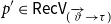
$p' \in {\mathsf{RecV}}_{(\overrightarrow {\vartheta } \to \tau )}$
is a fresh recursion variable; -
− for each part
$X_i$
of
$\overrightarrow {X}$
in (
$\gamma^{*}$
) (i.e., for each
$X_i \equiv A_i$
in
$\overrightarrow {X} \equiv \overrightarrow {A}$
, and each
$X_i \equiv B_i$
in
$\overrightarrow {X} \equiv \overrightarrow {B}$
),
$X'_i$
is the result of the free replacements
$X'_i \equiv X_i\{ p(\overrightarrow {u})(v) :\equiv p'(\overrightarrow {u}) \}$
of all occurrences of
$p(\overrightarrow {u})(v)$
by
$p'(\overrightarrow {u})$
(in the free occurrences of
$p$
), modulo renaming the variables
$\overrightarrow {u}, v$
, for
$i \in \{0, \ldots , n_X \}$
, that is,(30)
\begin{align} \overrightarrow {X'} \equiv \overrightarrow {X}\{ p(\overrightarrow {u})(v) :\equiv p'(\overrightarrow {u}) \} \end{align}
-








Definition 9 (
$\gamma ^*$
-Condition).

Assume that, for all
 $i=1, \ldots , n$
(
 $n \geq 0$
),
 $\tau , \vartheta , \vartheta _i \in {\mathsf{Types}}$
,
 $v, u_i \in {\mathsf{PureV}}$
,
 $p \in {\mathsf{RecV}}$
, and
 $P \in {\mathsf{Terms}}$
are such that
 $v : \vartheta$
,
 $u_i : \vartheta _i$
,
 $p : (\overrightarrow {\vartheta } \to (\vartheta \to \tau ) )$
,
 $P : \tau$
, and thus,
 $\lambda (\overrightarrow {u}^{\overrightarrow {\vartheta }} ) \lambda (v^{\vartheta }) (P^{\tau }) : (\overrightarrow {\vartheta } \to (\vartheta \to \tau ) )$
.
A recursion term
 $A \in {\mathsf{Terms}}$
satisfies the
 $\gamma ^*$
-condition for an assignment
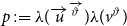 $p := \lambda (\overrightarrow {u}^{\overrightarrow {\vartheta }} ) \lambda (v^{\vartheta }) $
 $(P^{\tau }) :(\overrightarrow {\vartheta } \to (\vartheta \to \tau ) )$
, with respect to
 $\lambda (v)$
, if and only if
 $A$
is of the form (31):
 \begin{align} A &\equiv A_{0}\,\mathsf{where}\, \lbrace \overrightarrow {a} := \overrightarrow {A}, \, p := \lambda (\overrightarrow {u}) \lambda (v)P, \overrightarrow {b} := \overrightarrow {B}\! \rbrace \end{align}
with the subterms of appropriate types, such that the following holds:
-
(1)
$P \in {\mathsf{Terms}}_{\tau }$
does not have any free occurrences of
$v$
, that is,
$v \not \in {\mathsf{FreeV}}(P)$
-
(2) All occurrences of
$p$
in
$A_{0}$
,
$\overrightarrow {A}$
, and
$\overrightarrow {B}$
:-
(a) are free in
$A_{0}$
,
$\overrightarrow {A}$
, and
$\overrightarrow {B}$
, that is, not in the scope of
$\,\mathsf{where}\,$
-recursion assignments;
-
(b) are occurrences in subterms
$p(\overrightarrow {u})(v)$
, which are in a binding scope of
$\xi (v)$
, for
$\xi \in \{ \lambda , \exists , \forall \}$
, modulo renaming bound variables
$\overrightarrow {u}, v$
,
$i=1, \ldots , n$
(
$n \geq 0$
).
-


Note: the latter requirement (b) maintains the sets of the free variables of the terms
 $A$
by the
 $\gamma ^*$
reductions.
The additional reduction (
 $\gamma^{*}$
) rule is introduced in Loukanova (Reference Loukanova, van den Herik and Rocha2019c) and extends the reduction calculus of
 $\operatorname {L^{\lambda }_{ar}}$
of Moschovakis (Reference Moschovakis2006), by reducing the complexity of the terms and their algorithmic semantics.
The more simple
 $\gamma$
-rule introduced in Loukanova (Reference Loukanova2019b) is a special case of the (
 $\gamma^{*}$
) rule. Both rules,
 $\gamma$
- and
 $\gamma ^{*}$
, simplify terms, by reducing subterms that have superfluous
 $\lambda$
-abstractions,
 $p := \lambda (v) P$
, for
 $v \not \in {\mathsf{FreeV}}(P)$
, and corresponding functional applications
 $p (T)$
that have constant values. The (
 $\gamma^{*}$
) rule is more versatile and more useful than the
 $\gamma$
-rule for such algorithmic simplifications. A sequence of multiple consecutive
 $\lambda$
-abstractions in an assignment part
 $p := \lambda (\overrightarrow {u}) \lambda (v) P$
of a recursion term
 $A$
, for
 $u_{i} \in \overrightarrow {u}$
,
 $v \not \in {\mathsf{FreeV}}(P)$
, can be such that
 $\overrightarrow {u} \in {\mathsf{FreeV}}(P)$
. This prevents application of the simple
 $\gamma$
-rule with respect to
 $\lambda (v)$
in
 $p := \lambda (\overrightarrow {u}) \lambda (v) P$
. The (
 $\gamma^{*}$
) rule provides reducing
 $A$
by removing the vacuous
 $\lambda (v)$
with respect to
 $p := \lambda (\overrightarrow {u}) \lambda (v) P$
. The (
 $\gamma^{*}$
) rule does not alter algorithmic semantics of
 $\operatorname {L^{\lambda }_{ar}}$
and
 $\operatorname {L}^{\lambda }_{r}$
, in any other essential way.
Definition 10 (
$\gamma ^*$
-Reduction).

For all
 $A, B \in {\mathsf{Terms}}$
,
 $A \Rightarrow ^{*}_{\gamma ^*} B$
iff there is a sequence (including empty one) of consecutive, immediate reductions by (cong)–(
 $\gamma^{*}$
), that is:
 \begin{align} \begin{split} A \Rightarrow ^{*}_{\gamma ^*} B \iff &\textit{ there exist } A_{i} \in {\mathsf{Terms}}, 0 \leq i \leq n, \textit{ such that:} \\ & A \equiv A_{0}, \ A_{n} \equiv B, \textit{ and } \\ & A_{i} \Rightarrow A_{i+1}, \textit{ for some of the rules} (cong){-}(\gamma^{*}) \end{split} \end{align}
 \begin{align} \iff &\textit{ (abbreviated) } A \equiv A_{0} \Rightarrow \ldots \Rightarrow A_{n} \equiv B \ (n \geq 0) \end{align}
Often, we shall write
 $A \Rightarrow B$
instead of
 $A \Rightarrow ^{*}_{\gamma ^*} B$
, including when applying none or more than one rule. We shall avoide confusion between application of the individual (
 $\gamma^{*}$
) rule and any of the reduction rules. An application of the (
 $\gamma^{*}$
) rule to
 $A \in {\mathsf{Terms}}$
can be designated by
 $A {\Rightarrow _{(\gamma ^*)}} B$
, or by
 $A \Rightarrow ^{n}_{(\gamma *)} B$
when (
 $\gamma^{*}$
) rule has been applied
 $n$
(
 $n \geq 0$
) times.
Let
 $\operatorname {\mathfrak{A}}$
be a given semantic structure having a denotation function
 $ {\mathsf{den}}$
. In this paper, we do not include details about the denotational semantics and its denotation function. About such, see Moschovakis (Reference Moschovakis2006) and Loukanova (Reference Loukanova2019b, Reference Loukanova2023c, Reference Loukanova2023d, Reference Loukanova, Bekki, Mineshima and McCready2024).
For getting feeling of the essence of the (
 $\gamma^{*}$
) rule, we include the following statements.
Lemma 1.
Assume that, for
 $i=1, \ldots , n$
(
 $n \geq 0$
),
 $\tau , \vartheta , \vartheta _i \in {\mathsf{Types}}$
,
 $v, u_i \in {\mathsf{PureV}}$
,
 $p \in {\mathsf{RecV}}$
,
 $P \in {\mathsf{Terms}}_{\tau }$
,
 $v : \vartheta$
,
 $u_i : \vartheta _i$
,
 $p : (\overrightarrow {\vartheta } \to (\vartheta \to \tau ) )$
,
 $P : \tau$
,
 $p \not \in {\mathsf{FreeV}}(P)$
, and a given variable valuation
 $g$
is such that (34) holds:
 \begin{align} g (p) = & {\mathsf{den}} \bigl ( \lambda (\overrightarrow {u} ) \lambda (v) (P) \bigr ) (g) \end{align}
Then, for all
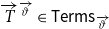 $\overrightarrow {T}^{\overrightarrow {\vartheta }} \in {\mathsf{Terms}}_{\overrightarrow {\vartheta }}$
,
 $T^{\vartheta } \in {\mathsf{Terms}}_{\vartheta }$
, such that
Footnote
1
 $v \not \in {\mathsf{FreeV}}(\overrightarrow {T})$
, the following (35a), (35b), and (36a)–(36c) hold:
 \begin{align} \lambda (\overrightarrow {u} ) \lambda (v) (P) \equiv {} & \lambda (\overrightarrow {u}^{\overrightarrow {\vartheta }} ) \lambda (v^{\vartheta }) (P^{\tau }) : (\overrightarrow {\vartheta } \to (\vartheta \to \tau ) ) \end{align}
 \begin{align} {\mathsf{den}} (p (\overrightarrow {T}) (T)) (g) = & {\mathsf{den}} \bigl ( \bigl [ \lambda (\overrightarrow {u} ) \lambda (v) (P) \bigr] (\overrightarrow {T}) (T) \bigr ) (g) \end{align}
Furthermore, assume that
 $v \not \in {\mathsf{FreeV}}(P)$
(as given in Definition
9
of the
 $\gamma ^*$
-Condition). Then, by the assumed types:
 \begin{align} {\mathsf{den}} \bigl ( \bigl [ \lambda (v) (P) \bigr] (T) \bigr ) (g) &= {\mathsf{den}}(P) (g) \end{align}
 \begin{align} {\mathsf{den}}(p (\overrightarrow {T}) (T)) (g) &= {\mathsf{den}} \bigl ( \bigl [ \lambda (\overrightarrow {u} ) \lambda (v) (P) \bigr] (\overrightarrow {T}) (T) \bigr ) (g) \end{align}
 \begin{align} &= {\mathsf{den}} \bigl ( \bigl [ \lambda (\overrightarrow {u} ) (P) \bigr] (\overrightarrow {T}) \bigr ) (g) \end{align}
Proof. (35a) follows by Definition 2.
(35b) follows directly from (34).
(36a) and (36c) follow by the definition of the denotation function (which is not in the subject of this paper) in the semantic structure
 $\operatorname {\mathfrak{A}}$
.
Thus, (
 $\gamma^{*}$
) rule does not affect the denotational semantics of
 $\operatorname {L^{\lambda }_{ar}}$
and
 $\operatorname {L}^{\lambda }_{r}$
, that is,
Theorem 2.
In any given semantic structure
 $\operatorname {\mathfrak{A}}$
having a denotation function
 $ {\mathsf{den}}^{\operatorname {\mathfrak{A}}}$
:
 \begin{align} \begin{split} &\textit{ for all } A, A',\textit{ such that } A {\Rightarrow _{\gamma ^*}} A', \textit{ it holds that:} \\ & {\mathsf{den}}^{\operatorname {\mathfrak{A}}}(A) = {\mathsf{den}}^{\operatorname {\mathfrak{A}}}(A') \end{split} \end{align}
Proof.
By induction on the length of the reduction sequence
 $A {\Rightarrow _{\gamma ^*}} A'$
, using the definition of the denotation function
 $ {\mathsf{den}}^{\operatorname {\mathfrak{A}}}$
, and Lemma 1. The essential induction step is in applying the (
 $\gamma^{*}$
) rule.
See the special case of the
 $\gamma$
-reduction in Loukanova (Reference Loukanova2019b).
See detailed motivations, examples, and properties of the (
 $\gamma^{*}$
) and
 $\gamma$
-rule in the papers that are devoted to these rules and the corresponding extended reduction calculi, see Loukanova (Reference Loukanova2019b, Reference Loukanova, van den Herik and Rocha2019c, Reference Loukanova2023c). Further motivations and examples of the utility of the (
 $\gamma^{*}$
) rule are provided in Loukanova (Reference Loukanova2016b, Reference Loukanova, Grabowski, Loukanova and Schwarzweller2020, Reference Loukanova2023b, Reference Loukanova2023d).
Definition 11 (
$\gamma ^*$
-Irreducible terms).

We say that a term
 $A \in {\mathsf{Terms}}$
is
 $\gamma ^*$
-
 $\mathrm{irreducible}$
if and only if (38) holds:
 \begin{align} \begin{split} \textit{ for all } B \in {\mathsf{Terms}}, \quad A \Rightarrow ^{*}_{\gamma ^*} B &\implies A \equiv _{\mathsf{c}} B \end{split} \end{align}
For any term
 $A$
that is
 $\gamma ^*$
-irreducible, we say that
 $A$
is irreducible.
Theorem 3 (Criteria for irreducibility).
With respect to the extended set of reduction rules:
-
(1) Every
$A \in {\mathsf{Consts}} \cup {\mathsf{Vars}}$
is irreducible.
-
(2)
$A(B)$
is irreducible iff
$B$
is immediate and
$A$
is explicit and irreducible.
-
(3)
$\lambda (x)(A)$
is irreducible iff
$A$
is explicit and irreducible.
-
(4)
$[A_{0} \,\mathsf{where}\, \{ \overrightarrow {p} := \overrightarrow {A} \}]$
is irreducible iff all parts
$A_{i}$
(
$i = 0, \ldots , n$
) are explicit and irreducible.
-
(5)
$\bigl (A_{0} \ {\mathsf{such\ that}}{}\ \{ \overrightarrow {C} \} \bigr )$
is irreducible iff all parts
$A_{0}$
,
$C_{i}$
(
$i = 0, \ldots , n$
) are immediate.






Proof. By structural induction on terms and checking the reduction rules.
4.3 Canonical forms of terms
We use the notation
 $ {\mathsf{cf}}_{\gamma ^*}(A) \equiv {\mathsf{cf}}(A)$
as in Definition 7 of the Canonical Forms of Terms.
Theorem 4 (Existence and uniqueness of canonical forms).
For every term
 $A \in {\mathsf{Terms}}$
, the following hold:
-
(1) (Existence of a
$\gamma ^*$
-canonical form of
$A$
) There exist explicit,
$\gamma ^*$
-irreducible
$A_{0}, \ldots , A_{n} \in {\mathsf{Terms}}$
(
$n \geq 0$
), such that the term
$ {\mathsf{cf}}_{\gamma ^*}(A)$
that is of the form (39) is
$\gamma ^{*}$
-irreducible, that is, irreducible and does not satisfy the
$\gamma ^{*}$
-condition in Definition
9
:(39)Thus,
\begin{align} {\mathsf{cf}}_{\gamma ^*}(A) &\equiv {} A_0 \,\mathsf{where}\, \lbrace p_1 := A_1 , \ldots , p_n := A_n \rbrace \end{align}
$ {\mathsf{cf}}_{\gamma ^*}(A)$
is
$\gamma ^*$
-irreducible.
-
(2)
$A$
and
$ {\mathsf{cf}}_{\gamma ^*}(A)$
have the same constants and free variables:
(40a)
\begin{align} {\mathsf{Consts}}(A) &= {\mathsf{Consts}}( {\mathsf{cf}}_{\gamma ^*}(A))\\[-10pt]\nonumber \end{align}
(40b)
\begin{align} {\mathsf{FreeV}}(A) &= {\mathsf{FreeV}}( {\mathsf{cf}}_{\gamma ^*}(A)) \end{align}
-
(3)
$A \Rightarrow ^{*}_{\gamma ^*} {\mathsf{cf}}_{\gamma ^*}(A)$
. -
(4) If
$A$
is
$\gamma ^*$
-irreducible, then
$A \equiv _{\mathsf{c}} {\mathsf{cf}}_{\gamma ^*}(A)$
. -
(5) If
$A \Rightarrow ^{*}_{\gamma ^*} B$
, then
$ {\mathsf{cf}}_{\gamma ^*}(A) \equiv _{\mathsf{c}} {\mathsf{cf}}_{\gamma ^*}(B)$
. -
(6) (Uniqueness of
$ {\mathsf{cf}}_{\gamma ^*}(A)$
modulo congruence) For every
$B \in {\mathsf{Terms}}$
, such that
$A \Rightarrow ^{*}_{\gamma ^*} B$
and
$B$
is
$\gamma ^*$
-irreducible, it holds that
$B \equiv _{\mathsf{c}} {\mathsf{cf}}_{\gamma ^*}(A)$
, that is
$ {\mathsf{cf}}_{\gamma ^*}(A)$
is unique, up to congruence. We write
(41)
\begin{align} A & {\Rightarrow _{\mathsf{cf}_{\gamma ^*}}} B \iff A \Rightarrow _{\mathsf{cf}} B \iff B \equiv_{{\mathsf{c}}} {\mathsf{cf}}_{\gamma ^*}(A) \equiv {\mathsf{cf}}(A) \end{align}





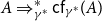





Proof.
The proof is by induction on term structure of
 $A$
, according to Definition 2, that is (3a)–(3h), using the notation that
 $ {\mathsf{cf}}_{\gamma ^*}(A) \equiv {\mathsf{cf}}(A)$
in the Definition 7 of the Canonical Forms of Terms, and reduction rules, of the extended
 $\gamma ^*$
-reduction relation.
Note: the reduction rules don’t remove or add any constants and free variables.
On the algorithmic semantics of the formal language of type-theory of recursion. The algorithmic meaning of a proper
 $A \in {\mathsf{Terms}}$
, that is, a non-immediate, algorithmically meaningful term, is designated by
 $ {\mathsf{alg}}(A)$
. It is determined by its canonical form
 $ {\mathsf{cf}}_{\gamma ^*}(A) \equiv {\mathsf{cf}}(A)$
.
Intuitively, for each proper
 $A\in {\mathsf{Terms}}$
, the algorithm
 $ {\mathsf{alg}}(A)$
for computing its denotation
 $ {\mathsf{den}} (A)$
consists of computation steps provided by the parts
 $A_{i}$
of its canonical form
 $ {\mathsf{cf}}(A) \equiv {A_0 \,\mathsf{where}\, \{p_1 := A_1, \ldots , p_n := A_n}\}$
, according to their
 $ {\mathsf{rank}} (A_{i})$
. Since the parts
 $A_{i}$
of the
 $ {\mathsf{cf}}(A)$
are explicit and irreducible, the computations for memorizing the values
 $ {\mathsf{den}}(A_{i})$
of the parts in the memory slots
 $p_{i}$
, by the assignments
 $p_{i} := A_{i}$
, are computationally the most basic. When the computational steps start from the lowest
 $ {\mathsf{rank}} (A_{i})$
, the algorithm for computing
 $ {\mathsf{den}}(A)$
is by iteration, that is, by recursive iteration.
For every
 $A \in {\mathsf{Terms}}$
, its canonical form
 $ {\mathsf{cf}}(A)$
, that is,
 $ {\mathsf{cf}}_{\gamma ^*}(A)$
, is obtained from
 $A$
by the reduction calculus of
 $\operatorname {L^{\lambda }_{ar}}$
, introduced in Section 4.2.
Definition 12 (Algorithmic equivalence).
See, for example, (Loukanova Reference Loukanova2023c). Assume a given semantic structure
 $\operatorname {\mathfrak{A}}$
. For all
 $A, B \in {\mathsf{Terms}}$
,
 $A$
and
 $B$
are
 $\gamma ^{*}$
-algorithmically equivalent, i.e., algorithmically synonymous in
 $\operatorname {\mathfrak{A}}$
,
 $A \approx _{\gamma ^*} B$
, iff
-
•
$A$
and
$B$
are both immediate, or
-
•
$A$
and
$B$
are both proper


and there are explicit,
 $\gamma ^{*}$
-irreducible terms (of appropriate, correspondingly the same types),
 $A_0$
, …,
 $A_n$
,
 $B_0$
, …,
 $B_n$
,
 $n \geq 0$
, such that:
-
(1)
$A \Rightarrow ^{*}_{\gamma ^*} A_{0} \,\mathsf{where}\, \{ p_1 := A_1, \ldots , p_n := A_n \} \equiv {\mathsf{cf}}_{\gamma ^*}(A)$
-
(2)
$B \Rightarrow ^{*}_{\gamma ^*} B_{0} \,\mathsf{where}\, \{ q_1 := B_1 , \ldots , q_n := B_n \} \equiv {\mathsf{cf}}_{\gamma ^*}(B)$
-
(3) for all
$i \in \{ 0, \ldots , n \}$
:(42a)
\begin{align} {\mathsf{den}}^{\operatorname {\mathfrak{A}}}(A_i)(g) &= {\mathsf{den}}^{\operatorname {\mathfrak{A}}}(B_i)(g),\ \textit{ for every variable valuation } g \in G\\[-10pt]\nonumber \end{align}
(42b)
\begin{align} {\mathsf{den}}^{\operatorname {\mathfrak{A}}}(A_i) &= {\mathsf{den}}^{\operatorname {\mathfrak{A}}}(B_i) \end{align}
-
(4) for all
$i \in \{ 0, \ldots , n \}$
:
$A_{i}$
and
$B_{i}$
have the same constants and free variables:
(43a)
\begin{align} {\mathsf{Consts}}(A_{i}) &= {\mathsf{Consts}}(B_{i})\\[-10pt]\nonumber \end{align}
(43b)
\begin{align} {\mathsf{FreeV}}(A_{i}) &= {\mathsf{FreeV}}(B_{i}) \end{align}




When
 $A \approx _{\gamma ^*} B$
, we say that
 $A$
and
 $B$
are algorithmically
 $\gamma ^*$
-equivalent, alternatively, that
 $A$
and
 $B$
are
 $\gamma ^*$
-synonymous in
 $\operatorname {\mathfrak{A}}$
. Often, we skip the label
 $\gamma ^{*}$
and mentioning
 $\operatorname {\mathfrak{A}}$
, when the context makes these clear, that is:
-
• We write
$A \approx B$
and
$ {\mathsf{cf}}(A) \approx {\mathsf{cf}}(B)$
, and say that
$A$
and
$B$
are algorithmically equivalent. -
• We write
$ {\mathsf{den}}(A) = {\mathsf{den}}(B)$
and
$A=B$
, and say that
$A$
and
$B$
are denotationally equivalent.





5. Feature-Structure Descriptions of the Terms in Syntax–Semantics Interface
In this paper, I use feature-value representations, that is, feature-structure descriptions of linguistic information in syntactic structures of NL expressions. I interleave syntactic information by corresponding semantic representations in analyses of syntax–semantic interfaces. For semantic representations in GCBLG, I shall use encoding of
 $\operatorname {L^{\lambda }_{ar}}$
terms by feature-value descriptions, similarly to Loukanova (Reference Loukanova, Bel-Enguix and Jiménez-López2011d, Reference Loukanova, Bel-Enguix, Dahl and Jiménez-López2011e). Furthermore, usually, I use feature-structure descriptions with
 $\operatorname {L^{\lambda }_{ar}}$
terms in canonical forms. This is significant for compactness and efficiency in compositional combinations of
 $\operatorname {L^{\lambda }_{ar}}$
terms.
That is, in what follows, I shall encode any given
 $A \in {\mathsf{Terms}}$
, as in (44a), by the feature-value description of type sem-cat that is the value of the feature sem in (44b):
 \begin{align} A & \equiv {} A_{0}^{\sigma _{0}} \, \,\mathsf{where}\, \, \{ p_1 := A_1^{\sigma _1}, \ldots , p_n := A_n^{\sigma _n} \} : \sigma _{0} \end{align}

The description pattern (44b) is a feature-structure description of a representation of
 $A \in {\mathsf{Terms}}_{\sigma _{0}}$
of the form (44a). Here, the term
 $A$
in (44a) renders a feature-structure description X of the GCBLG type syn-cat and is the value of the feature syn. The sequence of assignments
 $\{p_1 := A_1 , \ldots , p_n := A_n\}$
,
 $n \geq 0$
, represented by the value of the feature where, is an (acyclic) system of assignments in
 $\operatorname {L^{\lambda }_{ar}}$
. In general,
 $A_0 , \ldots , A_n \in {\mathsf{Terms}}$
, which are not necessarily explicit, irreducible terms. Thus, the reduction rules of the
 $\operatorname {L^{\lambda }_{ar}}$
can be applied to
 $A$
:
 $A \Rightarrow _{\mathsf{cf}} {\mathsf{cf}}(A)$
. The term
 $ {\mathsf{cf}}(A)$
is (representing) the algorithm for calculating
 $ {\mathsf{den}}(A)$
, and thus, the algorithm for computing the semantic denotation of X:
 \begin{align} A &\Rightarrow _{\mathsf{cf}} {\mathsf{cf}}(A)\\[-10pt]\nonumber \end{align}
 \begin{align} {\mathsf{den}}(A) &= {\mathsf{den}}( {\mathsf{cf}}(A))\\[-10pt]\nonumber \end{align}
 \begin{align} {\mathsf{cf}}(A) & \text{ is the algorithm for computing the semantic denotation of X} \end{align}
In case
 $A_0 , \ldots , A_n \in {\mathsf{Terms}}$
are explicit, irreducible, the semantic representation of X is
 $ {\mathsf{cf}}(A) \equiv {} A$
.
A feature structure of the form (44b) represents a rendering
 $\mathrm{X} \xrightarrow {\mathsf{render}} A$
. The
 $\operatorname {L^{\lambda }_{ar}}$
term
 $A$
encoded in (44b) can be in canonical form, which we will primary use in this paper:
 \begin{align} A \equiv {\mathsf{cf}}(A) \equiv A_0 \,\mathsf{where}\, \{p_1 := A_1 , \ldots , p_n := A_n\} \end{align}
6. Lexical Rules
Similarly to Sag et al. (Reference Sag, Wasow and Bender2003), we can use lexical rules for deriving new lexical items, by starting with a set of basic entries in a lexicon. Inflected forms of lexemes are licensed by instances of inflection rules. The syntactic rules provide necessary syntactic information for classification of the lexicon and for licensing co-occurrence distribution of the lexical items in the well-formed phrases. I use the feature-structure descriptions for semantic representations by rendering of the lexical items into
 $\operatorname {L^{\lambda }_{ar}}$
terms. For this, I use feature-value representations of
 $\operatorname {L^{\lambda }_{ar}}$
terms, as introduced in Loukanova (Reference Loukanova, Bel-Enguix and Jiménez-López2011d, Reference Loukanova, Bel-Enguix, Dahl and Jiménez-López2011e). The most general type for all lexical rules is represented by the type l-rule declared with a feature-structure constraint as in Sag et al. (Reference Sag, Wasow and Bender2003). and Loukanova (Reference Loukanova, Bel-Enguix and Jiménez-López2011d). For self-containment, I repeat the constraint of l-rule in (47). The constraint l-rule defines a relation between pairs of input and output lexical items. The input and output lexical items are pairs of type l-sequence
 $\langle X, F \rangle$
, where X is a can be a phonological form (represented by sound for voiced speech or an orthographical form for written) and
 $F$
is a feature structure of some specific subtype of lexeme or word. The feature-structure description [sem /
 $\boxed {1}$
] in the input and output values in (47) is a partial constraint, where the slash “/” designates that, by default, the input and output semantic representations are the same
 $\boxed {1}$
, unless some more specific lexical rule overrides this and changes the value
 $\boxed {1}$
of the feature sem, for example, by adding more semantic information to
 $\boxed {1}$
.

In this paper, I use the lexical subtypes i-rule and d-rule of the lexical type l-rule. Derivational rules of type d-rule are needed to licence passive, present, and past participles and other classes of lexemes.
Inflectional rules. Inflected lexemes are of type word and are ready for use in grammar rules for phrasal structures. Their feature-structure descriptions are licensed as outputs of instances of lexical rules that are subtypes of i-rule. The general constraint associated with the type i-rule is the same as in Sag et al. (Reference Sag, Wasow and Bender2003) and Loukanova (Reference Loukanova, Bel-Enguix and Jiménez-López2011d).
Lexical derivational rules. Some words are complex lexical items that are derived from more basic lexemes before they go through inflectional rules. The inflected forms may or may not vary in shape and may be the same as the input basic lexemes. For example, past and present participles are lexemes that are derived from verb lexemes. There is linguistic reason that the participles, as words, have distinguished inflectional forms, even though, as, for example, in English, for many common verbs, they may have the same, constant shape. Initially, lexemes that are derived from more basic lexemes, by instances of the type d-rule declared by the constraint (48)(a), are of type lexeme. Then, the derived lexemes of type lexeme undergo the inflectional rules, which output inflected lexemes of type word. This is so even in cases when the shape of the output form X’ is the same as that of the form X of the input lexeme. Such lexemes are licensed by the Constant Lexeme Lexical Rule, (48)(b), which is discussed in more details in Sag et al. (Reference Sag, Wasow and Bender2003).

Furthermore, the lexicon has two more constraints that propagate information into the phrasal structures. The Argument Realization Principle (ARP) is a constraint on the type word, which propagates linguistic data from arg-st of the word, which is order-independent into the syntactic features spr and comps, which get saturated according to order determined by the syntactic rules. Thus, arp provides syntax–semantics interface from lexemes into phrases.
The lexemes of type infl-lxm have to satisfy the constraint shac, by which the value of the feature head has to be with the same agreement value
 $\boxed {1}$
as that of the specifier:

7. The Passive Lexical Rule
In this paper, I follow the syntactic treatment of the passive construction in Sag et al. (Reference Sag, Wasow and Bender2003), which distinguishes the passive forms of verbs as specialized, derived lexemes that are participles of passive form. This can be achieved by a derivational lexical rule of subtype d-rule, for passivisation, as in (50), which outputs type participle lexeme, abbreviated as part-lxm, where the passive form of the verb is distinguished (from the past participle, which may have the same appearance) by a special feature form, which takes an atomic value pass (it can be denoted without abbreviation by passive).

where
 $\boxed {A}$
is a list of feature-structure descriptions and
 $\oplus$
is the operation of appending lists. By the Passive Lexical Rule (50), the arg-str of the input transitive verb in active form, of type tv-lxm is converted into the lexeme of type part-lxm for participle lexeme. The feature-value [head [form pass]] provides the linguistic information that the syntactic head of the output lexeme is passive participle. The effect of the passivisation rule (50) is reordering of the list arg-st of the arguments of the lexeme: the complement list
 $\boxed {A}$
is “moved” forward so that its first element takes the position of the spr of the passive form. The subject of the head verbal structure, the spr of the active verb form, that is, np [sem /
 $\boxed {1}$
] becomes optional complement of the syntactic category pp by the verbal argument marking preposition “by.” The optionality of the syntactic expression of the PP “(by [X]
 $_{\mathrm{NP}}$
)” is presented by including it in parentheses.
The val feature of the PP has comps value, which is the complement of the preposition “by”: “[form by] [val comps
 $\langle\, \boxed {2}\,\rangle$
]”
That is, the complement of the preposition “by” is the same
 $\boxed {2}$
NP as the first element of the arg-st of the active verb, which is the value of its spr, by the shac constraint (49).
8. Algorithmic Syntax–Semantics Interface of Active–Passive Correspondences
In this section, I present the ideas of key syntax–semantics relations between active and passive forms of verbal expressions. The head verb of an active sentence that can undergo passivization typically denotes a relation, for example, of action. The verb has at least two syntactic arguments and corresponding semantic argument roles, for example, it has a subject argument filled up by an expression, typically a NP designating the “agent” of the action and a complement denoting a “patient.” I introduce the method of using the type-theory
 $\operatorname {L^{\lambda }_{ar}}$
in algorithmic syntax–semantics interfaces between active and passive forms in NL.
Such algorithmic syntax–semantics interfaces utilize the algorithmic facilities of
 $\operatorname {L^{\lambda }_{ar}}$
, that is, its terms for semantic representations, its reduction calculi, and its theoretical results in the algorithmic information and computations.
For clarifications, at first, I demonstrate the method with a specific simple example, which while simple is a pattern representative of a large class of NL expressions. The general pattern has syntactic structure represented by syntactic tree structures encoded by brackets labeled by NL syntactic categories:
 \begin{align} & [[\unicode{x1D6F7}]_{\mathrm{NP}} \ [[\chi]_{\mathrm{V}} \ [\unicode{x1D6F9}]_{\mathrm{NP}}]_{\mathrm{VP}}]_{\mathrm{S}}\\[-10pt]\nonumber \end{align}
 \begin{align} & [[\mathrm{Mary}]_{\mathrm{NP}} [[\mathrm{likes}]_{\mathrm{V}} [\mathrm{Jim}]_{\mathrm{NP}}]_{\mathrm{VP}}]_{\mathrm{S}}\\[-10pt]\nonumber \end{align}
 \begin{align} & \mathrm{[[Kim]_{\textrm {NP}}\ [gave\ [Fido]_{\textrm {NP}}\ [to\ John]_{\textrm {PP}}]_{\textrm {VP}}]_{\textrm {S}} } \end{align}
Note that these specific proper names and verbs are instances of large NL classes and can be replaced with any other similar or more complex instances.
The feature-value description of the Passive Lexical Rule given in (50) is based on the key characteristics of the syntax–semantics relations between the syntactic and semantic argument roles of the verbal lexemes that will propagate into VPs and sentences.
The verbal lexemes undergo syntactic changes of the argument structure arg-str of the verb in active form and its corresponding passive form by the swap of the syntactic slots of the verbal lexeme, that is,
-
(1) Syntactic restructure
-
(a) The expression filling up one of the complement argument slots of the verb in active form (typically the first, direct complement) gets “moved” and filles up the subject slot of the passive verbal form.
-
(b) The filler of the verbal subject in the active verbal form takes the slot of the “moved” complement of the passive verbal form, for example, via a PP[form by] headed by a preposition like “by,” or optionally is skipped.
The syntactic restructure in English passivization is marked by a copula verb, for example, “be” and “get,” which also carries semantic information via inflection manifestation and grammatical agreement.
-
-
(2) The core semantic information is preserved and carried on, even when a semantic role becomes unexpressed, for example, that of the agent in the sentence in active form. The swap of the syntactic arguments does not change the semantic relation denoted by the verbal lexeme and its corresponding semantics argument slots.
8.1 Core semantic equivalence of a transfer between active and passive forms
The term
 $M_{0}$
in (52b) is a standard translation of such a sentence in lambda-calculi and in logic. The significance that
 $\operatorname {L^{\lambda }_{ar}}$
adds to it is that this terms can be reduced to its canonical form in
 $\operatorname {L^{\lambda }_{ar}}$
that designates the algorithmic steps in computing its denotation:
 \begin{align} &\text{ Mary liked Jim} \xrightarrow {\mathsf{render}}{} M_{0}\\[-10pt]\nonumber \end{align}
 \begin{align} M_{0} \equiv {} & [\textit{liked} (\textit{jim})](\textit{mary})\\[-10pt]\nonumber \end{align}
 \begin{align} \Rightarrow {} \ldots \Rightarrow {} {\mathsf{cf}}(M_{0}) \equiv {} & \textit{liked} (j)(m) \,\mathsf{where}\, \{ j := \textit{jim}, \, m := \textit{mary} \}\\ &\text{ by 2x(ap) twice, (rec-comp), (recap), (head)}\nonumber \end{align}
In (53a) and (53b), I present another randering of the same sentence in the active form, (52a), to a different
 $\operatorname {L^{\lambda }_{ar}}$
term
 $ {\mathsf{cf}}(T)$
, in (53b), which provides a generalization to a parametric algorithm for computing denotations of classes of sentences via instantiations:
 \begin{align} &\text{ Mary liked Jim} \xrightarrow {\mathsf{render}}{} {\mathsf{cf}}(T)\\[-10pt]\nonumber \end{align}
 \begin{align} T \equiv {} & [L (\textit{jim})](\textit{mary}) \,\mathsf{where}\, \{ L := \textit{liked} \}\\[-10pt]\nonumber \end{align}
 \begin{align} \Rightarrow {} \ldots \Rightarrow {} {\mathsf{cf}}(T) \equiv {} & L (j)(m) \,\mathsf{where}\, \{ L := \textit{liked}, \, j := \textit{jim}, \, m := \textit{mary} \}\\ &\text{ by 2x(ap) twice, (rec-comp), (recap), (head)}\nonumber \end{align}
As a first option, let’s assume that the sentence (54a) in passive form is rendered to the term (54b), where the order of the
 $\lambda$
-abstractions over the arguments provides correspondence to the reordering of the syntactic arguments in (54a).
Corollary 1.
The terms
 $B$
and
 $T$
in (54b) and (54c) are algorithmically equivalent,
 $B \approx {} T$
:
 \begin{align} &\textit{ Jim is liked by Mary} \xrightarrow {\mathsf{render}}{} B \equiv {} {\mathsf{cf}}(B)\\[-10pt]\nonumber \end{align}
 \begin{align} \begin{split} B \equiv {} & \bigl ( \lambda y_{m} \lambda x_{j} L (x_{j}) (y_{m}) \bigr ) (m) (j) \,\mathsf{where}\, \{ \\ & \qquad\quad\qquad L := \textit{liked}, \, j := \textit{jim}, \, m := \textit{mary} \} \end{split}\\[-10pt]\nonumber \end{align}
 \begin{align} B \approx {} T \equiv {} & L (j)(m) \,\mathsf{where}\, \{ L := \textit{liked}, \, j := \textit{jim}, \, m := \textit{mary} \} \end{align}
Proof.
The head parts of
 $B$
and
 $T$
in (54b) and (54c) are denotationally equivalent, by two denotational
 $\beta$
-conversions, that is,
 \begin{align} & \bigl ( \lambda y_{m} \lambda x_{j} L (x_{j}) (y_{m}) \bigr ) (m) (j) = L (j)(m) \end{align}
The terms
 $B$
and
 $T$
are proper, and their corresponding parts are explicit, irreducible, and denotationally equivalent. Therefore, by Definition 12, it follows that
 $B \approx {} T$
.
Note 4. The term
 $B$
in (54a)–(54c) cannot be reduced to
 $T$
by the reduction rules of
 $\operatorname {L^{\lambda }_{ar}}$
. The algorithmic equivalence in (54b) and (54c) is not by algorithmic
 $\beta$
-conversion. On the other hand,
 $\beta$
-conversion holds denotationally, which is valuable, for checking algorithmic equivalences between terms in irreducible canonical forms, by Definition 12. The algorithmic equivalence stated in Definition 12 depends on the denotational equalities between terms parts.
The canonical form
 $ {\mathsf{cf}}(T)$
of the active sentence in (53a) is algorithmically equivalent of the canonical form
 $ {\mathsf{cf}}(B)$
, by the above renderings, that is,
 \begin{align} B \approx {}& {\mathsf{cf}}(B) \equiv {} T \equiv {} {\mathsf{cf}}(T) \approx {} T \end{align}
This may seem as if being a discrepancy, but the important is that none of the terms
 $T \equiv {} {\mathsf{cf}}(T) \approx T$
is per se syntactically equivalent to
 $B \approx {} {\mathsf{cf}}(B)$
. There is formal syntactic difference between the canonical forms of the
 $\operatorname {L^{\lambda }_{ar}}$
terms rendering the corresponding active
 $ {\mathsf{cf}}(T)$
and passive
 $ {\mathsf{cf}}(B)$
forms.
The algorithmic equivalence
 $B \approx {} T$
, via (56), reflects on important linguistic information in NL, that is, the essential, core semantic event designated by a typical passive form of a sentence is the same as that of the corresponding active one. In the next sections, I show that the recursion variables and reduction calculus of
 $\operatorname {L^{\lambda }_{ar}}$
provide facility for algorithmic distinction between the active and passive expressions of the core semantic event in them, via the passivization role of the passive copula be. It is a passivization marker that blocks, that is, prevents the (second)
 $\beta$
-conversion over the semantic argument role that gets passivized, that is, over the one which is designated by the complement of the active sentence and promoted to the subject in the passive one.
9. The Passive be
In the syntax, the passive verb “be” takes as its complement a VP[form pass] in passive form headed by a passive participle. Both, the verb “be” and its verbal complement share the sentence subject, as a common syntactic and semantic argument. Another important role of the copula verb “be” is that its verbal inflection can carry semantic information about the time of the action denoted by the VP[form pass]. In Section 10, I show how that can be done with a pattern example, in two different ways: either by conjunction or by restrictor subterm. I consider the option by restrictor as superior to the conjunction because the information about the time is not a directly predicated part of the sentence predication.
The major role of the copula verb “be” in the syntax–semantics interface relation of the passivization is accomplished by rendering the lexeme “be” to a
 $\operatorname {L^{\lambda }_{ar}}$
constant
 $\textit{be}$
. The core of the semantic denotation of
 $\textit{be}$
is a function that takes the property denoted by the term rendering its VP[form pass] complement, that is, a verbal phrase VP[form pass] that is headed by a passive participle, and preserves it. By this, denotationally, the passivization preserves the semantic relations between objects denoted by the active sentences and keeps track of the correspondences between syntactic and semantic arguments.
9.1 The verb “be” as a passivization marker
When the lexeme “be” enters into a phrasal structure of a passive sentence, the function denoted by the constant
 $\textit{be}$
applies to and preserves the same property (the action)
 $X$
of type
 $(\tilde {\mathsf{e}} \rightarrow \tilde {\mathsf{t}})$
, which is designated by the syntactic complement (i.e., the passive VP[form pass]) of the lexeme “be,” acting over entities of type
 $\tilde {\mathsf{e}}$
, designated by the sentence subject.
For the purposes of this paper, that is, syntax–semantics of passivization in English, expressed by feature-value description (74), I assume that the lexeme “be” is rendered to a
 $\operatorname {L^{\lambda }_{ar}}$
-constant
 $\textit{be}$
that denotes the identity function over properties denoted by
 $X \in {\mathsf{Terms}}_{(\tilde {\mathsf{e}} \rightarrow \tilde {\mathsf{t}})}$
. The denotation
 $ {\mathsf{den}}(\textit{be})$
is expressed by (57a)–(57c), and similarly, for the inflected forms
 $\textit{is}$
,
 $\textit{was}$
, etc., if we suppress information about time carried by inflection:
 \begin{align} \begin{split} & \textit{be} \in {\mathsf{Consts}}_{((\tilde {\mathsf{e}} \rightarrow \tilde {\mathsf{t}}) \rightarrow (\tilde {\mathsf{e}} \rightarrow \tilde {\mathsf{t}}))}, \\ & \text{ such that, for a given }X \in {\mathsf{Terms}}_{(\tilde {\mathsf{e}} \rightarrow \tilde {\mathsf{t}})}\!: \textit{be} (X) = X \end{split}\\[-10pt]\nonumber \end{align}
 \begin{align} \begin{split} & \text{ i.e., for a given variable valuation $g$: } \\ & {\mathsf{den}}( \textit{be} (X) ) (g) = {\mathsf{den}}(\textit{be}) \bigl [ {\mathsf{den}}(X) \bigr] (g) = {\mathsf{den}}(X) (g) \end{split}\\[-10pt]\nonumber \end{align}
 \begin{align} &\textit{be} (X) = X \qquad \text{ iff } \qquad \textit{be} (X) {\models {\!|}} X \hspace {10ex} \text{ (denotational equality)}\\[-10pt]\nonumber \end{align}
 \begin{align} &\textit{is} (X) = X, \ \textit{was} (X) = X, \ldots \end{align}
That is, predicatively:
 $ {\mathsf{den}}( \textit{be} [ \textit{liked} (\textit{jim})] ) = {\mathsf{den}}( \textit{liked} (\textit{jim}) )$
, by suppressing tense information provided by inflection.
Compositionally, the sentence (58a) can be rendered as in (58b) and (58c). Then, by the reduction rules, we get (58f) and (58g) and its canonical form in (58l)–(58m):
 \begin{align} &\text{ Jim is liked by Mary} \end{align}
 \begin{align} \xrightarrow {\mathsf{render}}{} & A \equiv {} \Bigl [ \textit{is} \bigl [\underbrace { \underbrace {( \lambda y_{m} \lambda x_{j} L (x_{j}) (y_{m}) ) }_{ [\text{L-ed}]_{ [\textit {part-lxm pass}] } } (\textit{mary}) }_{\mathrm{[ L-ed\ by\ Mary]\, \textrm {VP}[\textit {pass}] }} \bigr] \Bigr] (\textit{jim}) \,\mathsf{where}\, \{ \end{align}
 \begin{align} & \hspace {40ex} L := \textit{liked} \} \end{align}
 \begin{align} \Rightarrow {} \ldots \Rightarrow {} A' \equiv {} & \bigl [ \textit{is} \bigl [( \lambda y_{m} \lambda x_{j} L (x_{j}) (y_{m}) ) (m) \ \bigr] \bigr] (j) \,\mathsf{where}\, \{\\[-10pt]\nonumber \end{align}
 \begin{align} & \hspace {20ex} L := \textit{liked}, \, j := \textit{jim}, \, m := \textit{mary} \}\\ &\text{ by 2x(ap) twice, (rec-comp), (recap), (head)} \nonumber\\[-8pt]\nonumber \end{align}
 \begin{align} \equiv {}& \underbrace { \bigl [ \textit{is} \bigl [\underbrace { \underbrace { ( \lambda y_{m} \lambda x_{j} L (x_{j}) (y_{m}) ) }_{[\text{L-ed}]_{ [\textit {part-lxm pass}] } \xrightarrow {\mathsf{render}}{} A_{0,0} } (m) }_{\text{ [L-ed by } m] \ \mathrm{VP}[\textit {pass}] \xrightarrow {\mathsf{render}}{} A_{0,1} } \bigr] \bigr] }_{\mathrm{ is } [\text{L-ed by } m] \textrm {VP}[\textit {pass}] \xrightarrow {\mathsf{render}}{} A_{0,2} } (j) \,\mathsf{where}\, \left \{\right . \end{align}
 \begin{align} & \hspace {20ex} \underbrace {L := \textit{liked}, \, j := \textit{jim}, \, m := \textit{mary}}_{\text{ specifications can be removed}}\! \left .\right \} \end{align}
 \begin{align} \Rightarrow {} & \Bigl [ [ \textit{is} (P)] \,\mathsf{where}\, \{ P := \bigl ( \lambda y_{m} \lambda x_{j} L (x_{j}) (y_{m}) \bigr ) (m) \} \Bigr] (j) \end{align}
 \begin{align} & \hspace {12ex} \,\mathsf{where}\, \{ \underbrace { L := \textit{liked}, \, j := \textit{jim}, \, m := \textit{mary} }_{\text{ specifications can be removed}} \}\\ &\text{ by (ap), (ap-comp), (rec-comp)}\nonumber \end{align}
 \begin{align} \Rightarrow {} & \Bigl [ [ \textit{is} (P)](j) \,\mathsf{where}\, \{ P := \bigl ( \lambda y_{m} \lambda x_{j} L (x_{j}) (y_{m}) \bigr ) (m) \} \Bigr] \end{align}
 \begin{align} & \hspace {12ex} \,\mathsf{where}\, \{ \underbrace { L := \textit{liked}, \, j := \textit{jim}, \, m := \textit{mary} }_{\text{ specifications can be removed}} \}\\ &\text{ by (recap), (rec-comp)}\nonumber \end{align}
 \begin{align} \Rightarrow {} & {\mathsf{cf}}(A) \equiv {} & \\ & [ \textit{is} (P)](j) \,\mathsf{where}\, \{ P := \underbrace {\bigl ( \lambda y_{m} \lambda x_{j} L (x_{j}) (y_{m}) \bigr ) (m), }_{\text{ [L-ed by $m$]} \ \mathrm{VP}[\textit {pass}] \xrightarrow {\mathsf{render}}{} A_{0,1}}\nonumber \end{align}
 \begin{align} & \hspace {18ex} \underbrace {L := \textit{liked}, \, j := \textit{jim}, \, m := \textit{mary} }_{\text{ specifications can be removed}} \}\\ &\text{ by (head)} \nonumber \\ \approx {} & M \equiv {} {\mathsf{cf}}(M) \equiv {} \nonumber \end{align}
 \begin{align} & P(j) \,\mathsf{where}\, \{ P := \underbrace {\bigl ( \lambda y_{m} \lambda x_{j} L (x_{j}) (y_{m}) \bigr ) (m), }_{\text{ [L-ed by $m$]} \ \mathrm{VP}[\textit {pass}] \xrightarrow {\mathsf{render}}{} A_{0,1} } \end{align}
 \begin{align} & \hspace {18ex} \underbrace {L := \textit{liked}, \, j := \textit{jim}, \, m := \textit{mary} }_{\text{ specifications can be removed}} \}\\ \nonumber &\text{ by (57d) for}\ \textit{is} (P) = P \end{align}
Optionally, instead of (58a) and (58b), we can render the same sentence (58a) directly to
 $ {\mathsf{cf}}(A)$
:
 \begin{align} &\text{ Jim is liked by Mary} \xrightarrow {\mathsf{render}}{} {\mathsf{cf}}(A) \end{align}
Passivization by “be” marker. In terms like (58b) and (58c) and (60a) and (60b), the
 $\operatorname {L^{\lambda }_{ar}}$
subterm
 $\textit{is}$
, which renders the passive copula, has a special role. It is a passivization “marker” that prevents denotational
 $\beta$
-substitution in the canonical forms. By this, it blocks algorithmic equivalence between passive and active renderings.
Now, let’s consider the term
 $R$
in (60a) and (60b), which is received from
 $A'$
in (58d) and (58e), by denotational
 $\beta$
-substitution of the bound variable
 $y_{m}$
with
 $m$
, in the head part of
 $A'$
. The terms
 $A'$
and
 $R$
are denotationally equivalent, that is,
 $A' = R$
, but we cannot directly conclude that
 $A \approx A' \approx R$
. We prove that this holds below.
By the reduction calculus of
 $\operatorname {L^{\lambda }_{ar}}$
, we have the following reductions of
 $R$
to its canonical form
 $ {\mathsf{cf}}(R)$
, and
 $R \approx {\mathsf{cf}}(R)$
:
 \begin{align} R & \equiv {} \bigl [ \textit{is} \bigl [\bigl( \lambda x_{j} \bigl [L (x_{j}) (m) \bigr] \bigr) \bigr] \bigr] (j) \,\mathsf{where}\, \{ \end{align}
 \begin{align} & \hspace {24ex} L := \textit{liked}, \, j := \textit{jim}, \, m := \textit{mary} \} \end{align}
 \begin{align} R & \equiv {} \underbrace { \bigl [ \textit{is} \bigl [\underbrace { ( \lambda x_{j} \bigl [L (x_{j}) (m) \bigr] ) }_{\text{[L-ed by }m] \mathrm{VP}[\textit {pass}] \xrightarrow {\mathsf{render}}{} R_{0,1} } \bigr] \bigr] }_{\text{ is [L-ed by }m] \mathrm{VP}[\textit {pass}] \xrightarrow {\mathsf{render}}{} R_{0,2} } (j) \,\mathsf{where}\, \{ \end{align}
 \begin{align} & \hspace {24ex} L := \textit{liked}, \, j := \textit{jim}, \, m := \textit{mary} \} \end{align}
 \begin{align} \Rightarrow {} & \bigl [ \textit{is} (R_{0,1}) \,\mathsf{where}\, \bigl\{ R_{0,1} := \lambda x_{j} \bigl [L (x_{j}) (m) \bigr] \bigr\} \bigr] (j) \,\mathsf{where}\, \{ \end{align}
 \begin{align} & \hspace {24ex} L := \textit{liked}, \, j := \textit{jim}, \, m := \textit{mary} \} \end{align}
 \begin{align} &\text{ by (ap) to the head subterm and (rec-comp)} \nonumber \\ \Rightarrow {} & \bigl [ \bigl [ \textit{is} (R_{0,1}) \bigr] (j) \,\mathsf{where}\, \bigl\{ R_{0,1} := \lambda x_{j} \bigl [L (x_{j}) (m) \bigr] \bigr\} \bigr] \,\mathsf{where}\, \{ \end{align}
 \begin{align} & \hspace {22ex} L := \textit{liked}, \, j := \textit{jim}, \, m := \textit{mary} \} \end{align}
 \begin{align} &\text{ by (recap) to the head subterm and (rec-comp)}\nonumber \\ \Rightarrow {} & \bigl [\textit{is} (R_{0,1} ) \bigr] (j) \,\mathsf{where}\, \{ R_{0,1} := \lambda x_{j} \bigl [L (x_{j}) (m) \bigr], \, \end{align}
 \begin{align} & \hspace {22ex} L := \textit{liked}, \, j := \textit{jim}, \, m := \textit{mary} \} \end{align}
 \begin{align} \nonumber &\text{ by (head)} \\ \Rightarrow {} {\mathsf{cf}}(R) \equiv {} & \bigl [\textit{is} (P ) \bigr] (j) \,\mathsf{where}\, \{ P := \lambda x_{j} \bigl [L (x_{j}) (m) \bigr], \, \end{align}
 \begin{align} & \hspace {22ex} L := \textit{liked}, \, j := \textit{jim}, \, m := \textit{mary} \} \end{align}
 \begin{align} \nonumber &\text{ by (cong) renaming of the bound } R_{0,1} \text{ to } P \\ \approx {} {\mathsf{cf}}(R') \equiv {} & \bigl [ P(j) \,\mathsf{where}\, \{ P := \lambda x_{j} \bigl [L (x_{j}) (m) \bigr], \, \end{align}
 \begin{align} & \hspace {22ex} L := \textit{liked}, \, j := \textit{jim}, \, m := \textit{mary} \}\\ \nonumber &\text{ by (57d) for } \textit{is} (P) = P \end{align}
Informally, the head term (60k)–(60l) expresses that
 $j$
is
 $P$
, where
 $P$
is [L-ed by
 $m$
], that is
 $j$
is liked by
 $m$
.
Corollary 2.
For the terms
 $A$
,
 $A'$
,
 $ {\mathsf{cf}}(A)$
,
 $R$
, and
 $ {\mathsf{cf}}(R)$
, respectively, in (58a)–(58m) and (60a)–(60j), the following algorithmic equivalences hold:
 \begin{align} A \approx {} A' \approx {} {\mathsf{cf}}(A) \approx {} R \approx {} {\mathsf{cf}}(R) \end{align}
Proof.
 \begin{align} {\mathsf{den}} \bigl ( \bigl [ \lambda y_{m} \lambda x_{j} L (x_{j}) (y_{m}) \bigr] (m) \bigr ) &= {\mathsf{den}} \bigl ( \lambda x_{j} L (x_{j}) (m) \bigr ) \end{align}
Therefore,
 $ {\mathsf{cf}}(A) \approx {} {\mathsf{cf}}(R)$
, by Definition 12.
9.2 Generalized parametric algorithms of passivization via passivization marker
From (58a), (58c)–(58d), and (53a)–(53c), by removing the specific instantiations of the lexical renderings into recursion variables for memory slots, we get the following algorithmic patterns, in canonical forms:
Algorithmic p
attern of a
ctive s
entences
. Let’s assume that the passivization copulas “be,” respectively inflected, are rendered into
 $\operatorname {L^{\lambda }_{ar}}$
terms:
 $\textit{be} \in {\mathsf{Consts}}_{((\tilde {\mathsf{e}} \rightarrow \tilde {\mathsf{t}}) \rightarrow (\tilde {\mathsf{e}} \rightarrow \tilde {\mathsf{t}}))}$
,
 $\textit{is}, \ \textit{was}, \ldots \in {\mathsf{Terms}}_{((\tilde {\mathsf{e}} \rightarrow \tilde {\mathsf{t}}) \rightarrow (\tilde {\mathsf{e}} \rightarrow \tilde {\mathsf{t}}))}$
.
Assume the following:
 $j, m \in {\mathsf{RecV}}_{\tilde {\mathsf{e} } }$
, which we use for saving in them values of terms rendering NPs denoting entities;
 $L \in {\mathsf{RecV}}_{( \tilde {\mathsf{e}} \rightarrow (\tilde {\mathsf{e}} \rightarrow \tilde {\mathsf{t}}) ) }$
, for saving the denotations of terms denoting two-argument relations, encoded by currying, that is, a class of relations of type:
 $( \tilde {\mathsf{e}} \rightarrow (\tilde {\mathsf{e}} \rightarrow \tilde {\mathsf{t}}) )$
.
We generalize the example rendering (53a)–(53c), by skiping the specific instantiations of lexemes, we get the following parametric algorithm for computing the denotations of a class of sentences with two-argument verbal head:
 \begin{align} & [ [\unicode{x1D6F7}]_{\mathrm{VP}} \ [ [\chi]_{\mathrm{V}} \ [\unicode{x1D6F9}]_{\mathrm{NP}}]_{\mathrm{VP}}]_{\mathrm{S}} \text{ (in active form)} \end{align}
 \begin{align} \xrightarrow {\mathsf{render}}{} & T \equiv {} {\mathsf{cf}}(T) \equiv {} L (j)(m) \end{align}
The general syntactic structures of sentences in active and corresponding passive form given in (63a) and (64a) are syntactic schemes that are syntactically parametric. In them,
 $\unicode{x1D6F7}$
,
 $\unicode{x1D6F9}$
, and
 $\chi$
are auxiliary symbols, that is, meta-variables, not belonging to the NL under analysis, neither to the formal language
 $\operatorname {L^{\lambda }_{ar}}$
. They represent any grammatical NL expressions of the syntactic categories given as indices to the brackets.
On the other hand, the expressions
 $L(j)(m)$
in (63b), and also in (64b)–(64e), abbreviated by
 $A, {\mathsf{cf}}(A), {\mathsf{cf}}(R), {\mathsf{cf}}(M)$
, are well-formed
 $\operatorname {L^{\lambda }_{ar}}$
terms. The recursion variables
 $j,m, L$
are free recursion variables, that is,
 $\operatorname {L^{\lambda }_{ar}}$
terms, rendering correspondingly
 $ [\unicode{x1D6F9}]_{\mathrm{NP}}$
,
 $ [\unicode{x1D6F7}]_{\mathrm{NP}}$
, the verbal expression
 $\chi$
. They have to be of suitable
 $\operatorname {L^{\lambda }_{ar}}$
types, otherwise are not specified.
Algorithmic p
attern of p
assive s
entences. From (58a) and (58b)–(58c), we get algorithmic patterns for computing the passive forms of the class of algorithms for the active sentences of the form (63a) and (63b). The specific algorithms are obtained by instantiations of the memory locations of the recursive variables
 $L$
,
 $m$
,
 $j$
:
 \begin{align} \begin{split} & [ [\unicode{x1D6F9}]_{\mathrm{NP}} \ [\text{is} \ [ [ F_{\textit{passprt}} ( \chi )]_{\mathrm{V} [\mathrm{FORM} \, passprt]} \\ & \hspace {20ex} \ \Bigl ( [\text{by} \ [\unicode{x1D6F7}]_{\mathrm{NP}}]_{{\mathrm{PP}}} \Bigr )]_{\mathrm{VP} [\mathrm{FORM} \, pass] }]_{\mathrm{VP}[\mathrm{FORM} \, pass]}]_{\mathrm{S}} \\ & \hspace {28ex} \text{ (in corresponding passive form)} \\ \xrightarrow {\mathsf{render}}{} & A / {\mathsf{cf}}(A) / {\mathsf{cf}}(R) / {\mathsf{cf}}(M) \kern50pt\text{ (optional renderings)} \end{split} \end{align}
 \begin{align} & A \equiv {} \bigl [ \textit{is} \bigl [ ( \lambda y_{m} \lambda x_{j} L (x_{j}) (y_{m}) ) (m) \bigr] \bigr] (j) \end{align}
 \begin{align} \Rightarrow {} & {\mathsf{cf}}(A) \equiv {} [ \textit{is} (P)](j) \,\mathsf{where}\, \bigr\{ P := \underbrace {\bigl ( \lambda y_{m} \lambda x_{j} L (x_{j}) (y_{m}) \bigr ) (m)}_{\text{ [L-ed by } m] \ \mathrm{VP}[\textit {pass}] \xrightarrow {\mathsf{render}}{} A_{0,1} } \bigl\} \end{align}
 \begin{align} \approx {} & {\mathsf{cf}}(R) \equiv {}\bigl [\textit{is} (P ) \bigr] (j) \,\mathsf{where}\, \bigr\{ P := \lambda x_{j} \bigl [L (x_{j}) (m) \bigr]\bigr\}\\[-10pt]\nonumber \end{align}
 \begin{align} \approx {} & {\mathsf{cf}}(M) \equiv {}\bigl [ P \bigr] (j) \,\mathsf{where}\, \bigl\{ P := \lambda x_{j} \bigl [L (x_{j}) (m) \bigr] \bigr\} \end{align}
Optionality of the PP c
omplement d
esignating the a
gent. We present the optional PP complement of the passives by inclosing that PP in parentheses. Note that the instantiations of the algorithmic patterns (64b)–(64e) by specific recursion assignments to the memory variables
 $j,m,L$
provided by specific instances of the semtence (64a).
See (78) for presenting the optionality of this PP in feature-structure description of the passive participle word “given” and examples of passive sentences.
In the cases when the optional PP complement [by
 $\unicode{x1D6F7}$
] is skipped, the corresponding semantic role of the verbal term must be saturated. The formal language of
 $\operatorname {L^{\lambda }_{ar}}$
has its unique facility to present this semantically, by filling the corresponding semantic role by its variables, which can be a free recursion variable
 $m$
as in (64b)–(64e) . The memory variable
 $m$
tentatively designating the agent and rendered by
 $\unicode{x1D6F7}$
remains underspecified without any instantiation of it, even after the other memory variables are instantiated.
We can generalize the patterns of renderings of the passive forms (64a) by any one of the following options, which are algorithmically equivalent:
-
(1) (64b)
Generalization of (58b)–(58c), by underspecification of the head verb, the subject, and the complement, and using the passivization marker
$\textit{is}$
in (64a) acting on the terms renderings:-
(a)
$\bigl [\textit{is} \bigl [ ( \lambda y_{m} \lambda x_{j} L (x_{j}) (y_{m}) ) (m) \bigr] \bigr]$
is rendering the passive VP:
$\chi \xrightarrow {\mathsf{render}} L$
to be instantiated by the head verbal participle;
$\unicode{x1D6F7} \xrightarrow {\mathsf{render}} m$
, to be instantiated by the rendering of
$\unicode{x1D6F7}$
. -
(b) the rendering of the promoted new subject
$j$
, to be instantiated by the rendering of
$\unicode{x1D6F9}$
.
-
-
(3) (64d) from (64c) by algorithmic equivalence via denotational
$\beta$
-conversion and by Definition 12. -
(4) (64e) from (64d) without the rendering
$\textit{is}$
of the copula verb “be,” by (57d) for
$\textit{is} (P) = P$
, but after it has completed its role as a passivization marker and by moving the rendering of the passive VP into the memory variable (slot)
$P$
.




Each one of the terms in the options (1)–(4) corresponds denotationally to the same core semantic event
 $L(j)(m)$
expressed by the active sentences of the form (63a)–(63b):
 \begin{align} {\mathsf{den}}(A) &= {\mathsf{den}}( {\mathsf{cf}}(A)) = {\mathsf{den}}( {\mathsf{cf}}(R)) = {\mathsf{den}}( {\mathsf{cf}}(M)) = L(j)(m)\\[-10pt]\nonumber \end{align}
 \begin{align} A &\approx {} {\mathsf{cf}}(A) \approx {} {\mathsf{cf}}(R) \approx {} {\mathsf{cf}}(M) \not \approx {} = L(j)(m) \end{align}
10. Verb Lexemes in Active Form
As a pattern of conversions, that is, similar to derivations, of verb lexemes and verbal phrases from active to passive form, I take a specific case of the verb “give.” I have chosen it because it has three syntactic arguments, and the semantic action
 $\textit{give}$
has three corresponding semantic argument roles (slots). In the syntax of a sentence in active form, with the head verb “give,” all three syntactic arguments are usually present. In a passive form of such a sentence, the syntactic argument expressed via a PP “by X” can be optionally skipped. However, the corresponding semantic argument role of
 $\textit{give}$
has to be filled up, saturated by a object designated by
 $X$
, or its underspecified semantic representative.
Other that special characteristics of the verbs like “give,” the technique that I present here, can be applied to any of a large class of verbs.
In this paper, we assume that the uninflected verb lexeme give, in active form, is rendered to a 3-argument
 $\operatorname {L^{\lambda }_{ar}}$
constant
 $\textit{givev}$
:
 \begin{align} \mathsf{give} & \xrightarrow {\mathsf{render}}{} \textit{give} \in {\mathsf{Consts}}_{( \tilde {\mathsf{e}} \rightarrow (\tilde {\mathsf{e}} \rightarrow (\tilde {\mathsf{e}} \rightarrow \tilde {\mathsf{t}})) )} \end{align}
Verb inflection by
 $\lambda$
-abstraction over variables for states. In (68a), the variable
 $u$
designates the (intended) state in which the lexeme give is used, for example, in a written or verbal utterance or abstract state, by which a predication is made. The value
 $\textit{lt} (u)$
is the space-time component of the state
 $u$
of using the passive sentence. The variable
 $s$
designates the state at which the “action” (abstract condition, property, relation, etc.), for example, the denotation of
 $give$
, is predicated to take place over some objects, for example,
 $y_{f}$
,
 $x_{j}$
, and
 $z_{k}$
. The time component of
 $s$
is the value
 $\textit{lt} (s)$
of the function
 $\textit{lt}$
and is the time of the “action.” Sometimes,
 $s$
is called the described state that is referred to by the utterance or by the statement made by
 $u$
, and we may call such a state
 $s$
predicate(ed) state. Note that
 $\lambda$
-abstraction over
 $s$
in (68a)–(68c) via (69a)–(69c) to (70a)–(70c) can facilitate the access to the state
 $s$
in
 $g(y_f)(x_j)(z_k) (s) :\mathsf{t}$
, since
 $\textit{give} : ( \tilde {\mathsf{e}} \rightarrow (\tilde {\mathsf{e}} \rightarrow (\tilde {\mathsf{e}} \rightarrow \tilde {\mathsf{t}})) )$
and
 $g(y_f)(x_j)(z_k) : (\mathsf{s} \to \mathsf{t}) \equiv \tilde {\mathsf{t}}$
:
The inflection in the verb forms can be expressed by conjunction or by restrictor. In (67a)–(67d), I show an option of representing inflection information by conjunction terms. After that, I shall demonstrate the inflectional restrictor.
Assume that
 $x_{j}, y_{f}, z_{k} \in {\mathsf{PureV}}$
. Strictly technically, the indices of these variables are irrelevant, and
 $x_{j}, y_{f}, z_{k}$
can be consistently replaced by any other variable letters, for example,
 $x, y, z$
. I use the indices as mnemonics for applications of
 $\lambda$
-terms to respective constants or recursion (memory) variables.
Assume that
 $s, u \in {\mathsf{Vars}}_{\mathsf{s}}$
. Here, we do not specify whether they are pure or recursion variables, as we allow both options. Pure variables can be abstracted over by
 $\lambda$
-abstraction terms, for example, (70a)–(70c).
On the other hand, both
 $s, u \in {\mathsf{RecV}}_{\mathsf{s}}$
can be left as underspecified recursion variables, that is, memory variables, that can be instantiated by specific instances of situations in given contexts, for example, as in (68a)–(68d).
Option 1: Underspecified predication states.
Option 1.1. We can render an inflected verb, like “gave,” into the term (67a)–(67d), by using a conjunction subterm for the time information, for example, in the past, by time precedence between time points or time of locations:
 \begin{align} \mathsf{gave} & \xrightarrow {\mathsf{render}}{} \lambda y_f \lambda x_j \lambda z_k \, \bigl ( g(y_f)(x_j)(z_k) (s) \land t \bigr ) \,\mathsf{where}\, \{ g := \textit{give}, \, \end{align}
 \begin{align} & \hspace {8em} t := (\textit{lt} (s) \prec \textit{ut}), \, \end{align}
 \begin{align} & \hspace {8em} \textit{lt} := \textit{time}, \, \textit{ut} := \textit{lt} (u) \} \end{align}
 \begin{align} & : ( \tilde {\mathsf{e}} \rightarrow (\tilde {\mathsf{e}} \rightarrow (\tilde {\mathsf{e}} \rightarrow \mathsf{t} )) ) \hspace {8ex} \text{ (underspecified states } u \text{ and } s ) \end{align}
Option 1.2. An inflected verb can be rendered to a
 $\operatorname {L^{\lambda }_{ar}}$
term by restrictor, for example, exemplified by the rendering (68a)–(68d):
 \begin{align} \mathsf{gave} & \xrightarrow {\mathsf{render}}{} \lambda y_f \lambda x_j \lambda z_k \, \bigl ( g(y_f)(x_j)(z_k) (s)\ {\mathsf{s.t.}}\ t \bigr ) \,\mathsf{where}\, \{ g := \textit{give}, \, \end{align}
 \begin{align} & \hspace {8em} t := (\textit{lt} (s) \prec \textit{ut}), \, \end{align}
 \begin{align} & \hspace {8em} \textit{lt} := \textit{time}, \, \textit{ut} := \textit{lt} (u) \} \end{align}
 \begin{align} & : ( \tilde {\mathsf{e}} \rightarrow (\tilde {\mathsf{e}} \rightarrow (\tilde {\mathsf{e}} \rightarrow \mathsf{t} )) ) \hspace {8ex} \text{ (underspecified states } u \text{ and } s ) \end{align}
Option 2
 $\lambda$
-attraction over predication state. Assume that
 $s \in {\mathsf{PureV}}_{\mathsf{s}}$
and
 $u \in {\mathsf{Vars}}_{\mathsf{s}}$
. We can take the inflected word “gave” to be rendered to the canonical form
 $ {\mathsf{cf}}(G)$
of the term
 $G$
. Here, the (
 $\xi$
) and (
 $\gamma^{*}$
) rules have significance in reductions to canonical forms. Namely, the rendering term (70a)–(70c), in canonical form, is the result of reductions of the term (69a)–(69c), by (
 $\xi$
)–(
 $\gamma^{*}$
), for
 $\xi \equiv \lambda$
:
 \begin{align} G \equiv {} & \lambda s \Bigl [ \bigl ( g(y_f)(x_j)(z_k) (s)\ {\mathsf{s.t.}}\ t \bigr ) \,\mathsf{where}\, \{ g := \textit{give}, \, \end{align}
 \begin{align} & \hspace {13.5em} t := (\textit{lt} (s) \prec \textit{ut}), \, \end{align}
 \begin{align} & \hspace {13.5em} \textit{lt} := \textit{time}, \, \textit{ut} := \textit{lt} (u) \} \, \Bigr]\\ \nonumber : \tilde {\mathsf{t}} \end{align}
Then, we can render an inflected verb, like “gave,” into the term (70a)–(70c):
 \begin{align} \mathsf{gave} \xrightarrow {\mathsf{render}}{} {\mathsf{cf}}(G) \equiv {} & \lambda y_f \lambda x_j \lambda z_k \lambda s \, \bigl ( g(y_f)(x_j)(z_k) (s)\ {\mathsf{s.t.}}\ t(s) \bigr ) \,\mathsf{where}\, \{ \end{align}
 \begin{align} & \hspace {8em} g := \textit{give}, \, t := \lambda s \, (\textit{lt} (s) \prec \textit{ut}), \, \end{align}
 \begin{align} & \hspace {8em} \textit{lt} := \textit{time}, \, \textit{ut} := \textit{lt} (u) \}\\ & : ( \tilde {\mathsf{e}} \rightarrow (\tilde {\mathsf{e}} \rightarrow (\tilde {\mathsf{e}} \rightarrow \tilde {\mathsf{t}} )) ) \hspace {6ex} \text{ (underspecified state } u)\nonumber \end{align}
Then, the sentence
 $\varPhi$
, which is in active form, can be rendered by (71b) or directly to the term in canonical form (71c):
 \begin{align} \varPhi \equiv {} & \mathrm{ [[Kim]_{\textrm {NP}}\ [gave\ [Fido]_{\textrm {NP}}\ [to\ John]_{\textrm {PP}}]_{\textrm {VP}}]_{\textrm {S}} } \end{align}
 \begin{align} \begin{split} \varPhi \xrightarrow {\mathsf{render}}{}& \bigl [ \lambda y_f \lambda x_j \lambda z_k \lambda s \, \bigl ( g(y_f)(x_j)(z_k) (s)\ {\mathsf{s.t.}}\ t(s) \bigr ) \\ & \hspace {8ex} \,\mathsf{where}\, \{ g := \textit{give}, \, \\ & \hspace {16.5ex} t := \lambda s \, (\textit{lt} (s) \prec \textit{ut}), \, \\ & \hspace {16.5ex} \textit{lt} := \textit{time}, \, \textit{ut} := \textit{lt} (u) \} \bigr] (\textit{fido}) (\textit{john}) (\textit{kim}) : \tilde {\mathsf{t}} \\ & \text{ (by compositional SynSem application of components)} \end{split} \end{align}
 \begin{align} \begin{split} \Rightarrow {} & \bigl [ \lambda y_f \lambda x_j \lambda z_k \lambda s \, \bigl ( g(y_f)(x_j)(z_k) (s)\ {\mathsf{s.t.}}\ t(s) \bigr ) \bigr] (\textit{fido}) (\textit{john}) (\textit{kim}) \\ & \hspace {8ex} \,\mathsf{where}\, \{ g := \textit{give}, \, \\ & \hspace {16.5ex} t := \lambda s \, (\textit{lt} (s) \prec \textit{ut}), \, \textit{lt} := \textit{time}, \, \textit{ut} := \textit{lt} (u) \} \\ & \text{ (by three times (recap))} \end{split} \end{align}
 \begin{align} \begin{split} \Rightarrow {} & \bigl [ \lambda y_f \lambda x_j \lambda z_k \lambda s \, \bigl ( g(y_f)(x_j)(z_k) (s)\ {\mathsf{s.t.}}\ t(s) \bigr ) \bigr] (f) (j) (k) \\ & \hspace {8ex} \,\mathsf{where}\, \{ g := \textit{give}, \, f := \textit{fido}, \, j := \textit{john}, \, k := \textit{kim}, \, \\ & \hspace {16.5ex} t := \lambda s \, (\textit{lt} (s) \prec \textit{ut}), \, \textit{lt} := \textit{time}, \, \textit{ut} := \textit{lt} (u) \} \\ & \text{ by several times (ap), (rec-comp), (head)} \end{split} \end{align}
Verb inflection and underspecified arguments. In (72a),
 $f, j, k \in {\mathsf{RecV}}_{\tilde {\mathsf{e}}}$
are free, underspecified memory variables, which have to be specified, in order to get a term that is specified by the rendering sentence components. Note that
 $u, s \in {\mathsf{Vars}}_{\mathsf{s}}$
are also free variables, which designate, correspondingly, the state
 $u$
of making a predication statment and the predication state
 $s$
. These states are not explicitly referred by overt sentential components, except inflection morphemes and agents’ references:
 \begin{align} \mathsf{gave} & \xrightarrow {\mathsf{render}}{} ( g(s) {\mathsf{s.t.}}\ t ) \,\mathsf{where}\, \{ g := \textit{give} (f)(j)(k), \, \end{align}
 \begin{align} & \hspace {14ex}t := (\textit{lt} (s) \prec \textit{ut}), \, \end{align}
 \begin{align} & \hspace {14ex}\textit{lt} := \textit{time}, \, \textit{ut} := \textit{lt} (u) \} : \mathsf{t} \end{align}
Then, the sentence
 $\varPhi$
can be rendered by (73b)–(73e):
 \begin{align} \varPhi \equiv {} & \mathrm{ [[Kim]_{\textrm {NP}}\ [gave\ [Fido]_{\textrm {NP}}\ [to\ John]_{\textrm {PP}}]_{\textrm {VP}}]_{\textrm {S}} } \end{align}
 \begin{align} \varPhi \xrightarrow {\mathsf{render}}{} & (g(s)\ {\mathsf{s.t.}}\ t ) \,\mathsf{where}\, \{ g := \textit{give} (f)(j)(k), \, \end{align}
 \begin{align} & \hspace {4.5em} f := \textit{fido}, \, j := \textit{john}, \, k := \textit{kim}, \, \end{align}
 \begin{align} & \hspace {4.5em} t := (\textit{lt} (s) \prec \textit{ut}), \, \end{align}
 \begin{align} & \hspace {4.5em} \textit{lt} := \textit{time}, \, \textit{ut} := \textit{lt} (u) \} : \mathsf{t} \end{align}
11. Syntax–Semantics Relations in Lexemes and Phrases in Passive Form
11.1 TTAA terms in syntax–semantics analysis of passives via feature-structure descriptions
The entry of the lexeme “be” can be given by a feature-structure description, for example, that in (74) (there may be other alternatives). The feature-structure description (74) represents a bare lexeme for the passive be, which is uninflected. It is a potential input to specific inflection rules:

Informally, in (74), the verb “be” has
 $\boxed {1}$
as its spr, by the feature-value description [spr
 $\langle$
 $\boxed {1}$
np [agr
 $\boxed {4}$
]
 $\rangle$
]. That is, the syntactic subject of the verb “be” is
 $\boxed {1}$
, which is the same as the subject [spr
 $\langle$
 $\boxed {1}$
 $\rangle$
] of its comps element
 $\boxed {2}$
. The lexeme “be” takes as a complement
 $\boxed {2}$
, expressed by the feature-value description comps
 $\langle$
 $\boxed {2}$
 $\rangle$
. And also,
 $\boxed {2}$
is the second argument element of its arg-st, by which
 $\boxed {2}$
is a VP in passive form and has a semantic representative of type
 $(\tilde {\mathsf{e}} \rightarrow \tilde {\mathsf{t}})$
.
The comps of “be” is not expressed explicitly in (74) because it is derived by the type constraints in syntax–semantics of feature-structure descriptions.
The word feature-structure description (76) for the past form of the passive be can be licensed by an inflectional lexical rule Past 3rd-Singular Tense Verb Lexical Rule, which is defined similarly to the Present Continuous 3rd-Singular Tense Verb Lexical Rule in Loukanova (Reference Loukanova, Bel-Enguix, Dahl and Jiménez-López2011e).
The underspecified
 $W^{((\tilde {\mathsf{e}} \rightarrow \tilde {\mathsf{t}}) \rightarrow (\tilde {\mathsf{e}} \rightarrow \tilde {\mathsf{t}}))} \in {\mathsf{Terms}}$
renders the inflected word “was,” where the inflection information is rendered by a conjunction in (75b). The underspecification of
 $W$
is for the referring (utterance) state
 $u$
;
 $ut$
is a location variable that saves the time of the referring (utterance) or predication state, via
 $\textit{ut} := \textit{lt} (u)$
:
 \begin{align} \mathsf{was} & \xrightarrow {\mathsf{render}} W \end{align}
 \begin{align} W & \equiv \lambda (v) \, \lambda (x) \, \lambda (s) \bigl [ w(v)(x)(s) \land t(s) \bigr] \,\mathsf{where}\, \{ w := \textit{be}, \, \end{align}
 \begin{align} & \hspace {8ex} t := \lambda (s) \bigl ( \textit{lt}(s) \prec \textit{ut} \bigr ) , \, \textit{lt} := \textit{time}, \, \textit{ut} := \textit{lt} (u) \} \end{align}
 \begin{align} & \hspace {2.5ex} : ((\tilde {\mathsf{e}} \rightarrow \tilde {\mathsf{t}}) \rightarrow (\tilde {\mathsf{e}} \rightarrow \tilde {\mathsf{t}})) \end{align}
In this section, we maintain the expression of the inflection of the passive was in the larger expressions by conjunction for the tense restrictions. Note that we can express this inflection information by restrictor terms, similarly to that in the active verbal forms in Section 10, which we use in Section 12.
The syntax–semantics interface of the underspecified passive word “was” can be represented by the feature-structure description (76), via suitable encoding of
 $W^{((\tilde {\mathsf{e}} \rightarrow \tilde {\mathsf{t}}) \rightarrow (\tilde {\mathsf{e}} \rightarrow \tilde {\mathsf{t}}))} \in {\mathsf{Terms}}$
as the value of the feature sem:

The feature-structure description (76) of the passive word “was” represents its underspecified syntax–semantics interface open for specifications by VPs in passive forms, where the verbal head can be instantiated by a passive participle.
In (75a)–(75c), the
 $\lambda (v)$
abstraction is over the passive verb phrase,
 $\lambda (x)$
is over the subject of the passive action (which is the complement in the active verbal phrase), the value
 $\textit{time} (s)$
is the time component of the state
 $s$
, and the value
 $\textit{time} (u)$
is the time component of the state
 $u$
of using the passive “be” expression.
In (75a)–(75c), and respectively (76), we may introduce the application of the head term, that is, of t-head term, to the free recursion variable
 $h \in {\mathsf{RecV}}_{(\tilde {\mathsf{e}} \rightarrow \tilde {\mathsf{t}})}$
as declaration, that is, reservation, of the free memory slot, of respective type, for passive VP having underspecified verbal passive participle. This memory slot can be specified by a class of VPs in passive form (where the verbal head is passive participle). Here, we refrain from this application to maintain the logic type of was.
11.2 Passive participle lexemes
In what follows, as a pattern for algorithmic syntax–semantics analysis of passive forms, I present two optional word feature structures of the passive participle lexemes “given,” (78) and (92), derived from the transitive lexeme give, for example, given in (77).
We can represent the syntax–semantics interface of the lexeme give by the feature-structure description (77):

The word pair consisting of a passive participle like “given” and its syntax–semantics interrelations can be represented by the feature-structure description (78):

Note that (77) is not restricted by the ARP, which applies to lexemes of type word, that is, the NP in the SPR list is not restricted to be identical to the first NP in the ARG-ST list. Then, there are two words “given” as the optional outputs of the Passive Lexical Rule followed by the Constant Lexeme Lexical Rule, (78) and (92). The word structure (78) has two complements in the COMPS list, where the feature description
 $\boxed {3}$
PP [syn [head [form by]]] represents the syntax–semantics information of the corresponding argument marking PP. Argument marking PPs can be presented by using a technique as in Loukanova and Jiménez-López (Reference Loukanova, Jiménez-López, Pérez, Sánchez, Mathieu, Rodríguez, Adam, Ortega, Moreno, Navarro, Hirsch, Lopes-Cardoso and Julián2012). The word structure (78) has two syntactic complements in its comps list, while the second one that is a PP is optional and can be skipped, for example, (92) has just one complement. In both cases, the
 $\operatorname {L^{\lambda }_{ar}}$
constant
 $\textit{give}$
has three semantic arguments:
 \begin{align} & \textit{give} \in {\mathsf{Consts}}_{( \tilde {\mathsf{e}} \rightarrow (\tilde {\mathsf{e}} \rightarrow (\tilde {\mathsf{e}} \rightarrow \tilde {\mathsf{t}})) )} \end{align}
 \begin{align} &\mathsf{given} \xrightarrow {\mathsf{render}} \ \big [\lambda x_j \lambda z_k \lambda y_f \, give(y_f)(x_j)(z_k)\big] \end{align}
Optionality of the PP complement designating the agent. In English, the subject of a sentence in active form, having as its verb head “give,” is a NP, which is obligatory. In a corresponding sentence of passive form this NP is transformed into the NP-head of a PP, [by NP]
 $_{\mathrm{PP}}$
. This PP is optionally skipped. I present this optionality by inclosing its corresponding feature-structure description
 $\boxed {3}$
in parentheses, in the argument-structure list value of arg-st (78).
On the other hand, the semantic argument role af the agent doing the action of the giving cannot be optional and has to be filled up, even if with unspecified variable. This is presented by the
 $\lambda$
-abstraction in the term rendering the verbal participle “given,” that is, by the variable
 $z_{k}$
in
 $give(y_f)(x_j)(z_k)$
. The passivization includes corresponding change of the order of saturating these three roles by the term
 $\big [\lambda x_j \lambda z_k \lambda y_f \, give(y_f)(x_j)(z_k)\big]$
. When the optional syntactic argument [by NP]
 $_{\mathrm{PP}}$
is skipped, the corresponding semantic one gets saturated by a recursion variable of
 $\operatorname {L^{\lambda }_{ar}}$
, that is, by well-formed
 $\operatorname {L^{\lambda }_{ar}}$
term.
Also, see the explanations on page 76.
11.3 Passive verb phrases
From the lexical rendering (79b), compositionally, one can get the rendering (80a)–(80c) of the passive VP having passive participle given as its head:
 \begin{align} &\mathsf{ [} \mathsf{ given\ [to\ John]}_{\mathrm{PP}}\ \mathsf{ [by\ Kim]}_{\mathrm{PP}}\mathsf{]}_{\mathrm{VP}} \xrightarrow {\mathsf{render}} \ C \end{align}
 \begin{align} C \equiv {} & \Bigl [ \bigl [\lambda x_j \lambda z_k \lambda y_f \, \bigl ( give(y_f)(x_j)(z_k) \bigr ) \bigr] (j) (k)\Bigr] \,\mathsf{where}\, \end{align}
 \begin{align} &\hspace {4em}\{j := \textit{john}, \, k := \textit{kim} \} : (\tilde {\mathsf{e}} \rightarrow \tilde {\mathsf{t}}) \end{align}
 \begin{align} H \equiv {} & \Bigl [ \bigl [\lambda x_j \lambda z_k \lambda y_f \, \bigl ( give(y_f)(x_j)(z_k) \bigr ) \bigr] (j) (k)\Bigr] {\models {\!|}} \lambda y_f \, \bigl ( give(y_f)(j)(k) \bigr ) \end{align}
 \begin{align} \ C {\models {\!|}}{} & D \equiv {}\lambda y_f \, \bigl ( give(y_f)(j)(k) \bigr ) \hspace {11ex} \text{ (denotational equality)} \\ &\hspace {3.5em}\{ j := \textit{john}, \, k := \textit{kim} \} \nonumber \end{align}
 \begin{align} C \approx {} & D \end{align}
The algorithmic equivalence
 $C \approx {} D$
in (80e), by Definition 12 and (80d).
Then, the passive VP (81a), in past tense, can be rendered by the term (81b)–(81f), via instantiation (81c) of the recursion variable
 $h \in {\mathsf{RecV}}$
in the term (81b)–(81f). Its syntax–semantics interface can be encoded by a corresponding feature-structure description:
 \begin{align} &\mathsf {[was\ [ given\ [to\ John]}_{\mathrm{PP}} \mathsf {[by\ Kim]}_{\mathrm{PP}} \mathsf {]}_{\mathrm{VP}} \mathsf {]}_{\mathrm{VP}} \xrightarrow {\mathsf{render}}{} E \end{align}
 \begin{align} E \equiv {} &\lambda v \, \lambda x \, \lambda s \, \bigl ( w(v)(x)(s) \land t (s) \bigr ) (h) \,\mathsf{where}\, \{ w := \textit {be} \end{align}
 \begin{align} &\hspace {3.7em} h := \Bigl [ \bigl [\lambda x_j \lambda z_k \lambda y_f \, give(y_f)(x_j)(z_k)\bigr](j)(k) \Bigr], \, \end{align}
 \begin{align} & \hspace {3.9em}j := \textit{john}, \, k := \textit{kim}, \, \end{align}
 \begin{align} & \hspace {3.8em} t := \lambda (s) (\textit{lt} (s) \prec \textit{ut}), \, \end{align}
 \begin{align} & \hspace {3.5em} \textit{lt} := \textit{time}, \, \textit{ut} := \textit{lt} (u) \} : (\tilde {\mathsf{e}} \rightarrow \tilde {\mathsf{t}}) \end{align}
11.4 Rendering sentences in passive form
Compositionally, from (81b)–(81f), the sentence (82a) in passive form is rendered to (82b)–(82f), by compositional application of the rendering (81a)–(81f) of the VP to the rendering
 $\textit{fido}$
of the subject [Fido]
 $_{\mathrm{NP}}$
:
 \begin{align} & \mathsf{ [ [Fido]}_{\mathrm{NP}}\ \mathsf{[was\ [ given\ [to\ John]}_{\mathrm{PP}}\ \mathsf{[by\ Kim]}_{\mathrm{PP}}\ \mathsf{]}_{\mathrm{VP}} \mathsf{]}_{\mathrm{VP}} \mathsf{]}_{\mathrm{S}} \xrightarrow {\mathsf{render}}{} A \end{align}
 \begin{align} &A \equiv {} \bigl [ \lambda v \, \lambda x \, \lambda s \, \bigl (w(v)(x)(s) \land t(s) \bigr )(h) \bigr] (f) \,\mathsf{where}\, \{ w := \textit {be}, \, \end{align}
 \begin{align} &\hspace {18ex} h := \Bigl [ \bigl [\lambda x_j \lambda z_k \lambda y_f \, give(y_f)(x_j)(z_k)\bigr](j)(k)\Bigr], \, \end{align}
 \begin{align} &\hspace {18.2ex} f := \textit{fido}, \, j := \textit{john}, \, k := \textit{kim}, \, \end{align}
 \begin{align} & \hspace {18.5ex} t := \lambda (s) (\textit{lt} (s) \prec \textit{ut}), \, \end{align}
 \begin{align} & \hspace {18ex} \textit{lt} := \textit{time}, \, \textit{ut} := \textit{lt} (u) \} : \tilde {\mathsf{t}} \end{align}
 \begin{align} & \mathsf{ [ [Fido]}_{\mathrm{NP}}\ \mathsf{[was\ [ given\ [to\ John]}_{\mathrm{PP}}\ \mathsf{[by\ Kim]}_{\mathrm{PP}} \mathsf{]}_{\mathrm{VP}} \mathsf{]}_{\mathrm{VP}} \mathsf{]}_{\mathrm{S}} \xrightarrow {\mathsf{render}}{} A \approx {} A_{1} \end{align}
 \begin{align} &A_{1} \equiv {} \bigl [ \lambda v \, \lambda x \, \lambda s \, \bigl (w(v)(x)(s) \land t(s) \bigr )(h) \bigr] (f) \,\mathsf{where}\, \{ w := \textit {be}, \, \end{align}
 \begin{align} &\hspace {18ex} h := \Bigl [ \bigl [ \lambda y_f \, give(y_f)(j)(k)\bigr]\Bigr], \, \end{align}
 \begin{align} &\hspace {18.2ex} f := \textit{fido}, \, j := \textit{john}, \, k := \textit{kim}, \, \end{align}
 \begin{align} & \hspace {18.5ex} t := \lambda (s) (\textit{lt} (s) \prec \textit{ut}), \, \end{align}
 \begin{align} & \hspace {18ex} \textit{lt} := \textit{time}, \, \textit{ut} := \textit{lt} (u) \} : \tilde {\mathsf{t}} \end{align}
The feature-structure description (84b) of the sentence (82a) renders the syntax–semantics interface of the sentence (84a) in passive form:
 \begin{align} & \varPsi \equiv \mathsf{ [ [Fido]}_{\mathrm{NP}}\ \mathsf{[was\ [ given\ [to\ John]}_{\mathrm{PP}}\ \mathsf{[by\ Kim]}_{\mathrm{PP}} \mathsf{]}_{\mathrm{VP}} \mathsf{]}_{\mathrm{VP}} \mathsf{]}_{\mathrm{S}} \xrightarrow {\mathsf{render}}{} F \end{align}

where
 $h : (\tilde {\mathsf{e}} \rightarrow \tilde {\mathsf{t}})$
stands for the (passive) predicate over
 $x \in {\mathsf{PureV}}_{\tilde {\mathsf{e}}}$
, and
 $s \in {\mathsf{PureV}}_{\mathsf{s}}$
is pure variable for
 $\lambda$
-abstraction over the state of the statement (described as the one in which giving may happen) expressed by the utterance, that is, the predication
 $u$
, which is designated by the free (underspecified memory variable)
 $u \in {\mathsf{RecV}}_{\mathsf{s}}$
.
Semantic suppression of the passive constant
 $\textit{was}$
. By (57c), we may skip the parameter
 $w$
and its assignment
 $w := \textit{be}$
in one of the optional renderings (85a), (85b), or (85c), and the corresponding feature-structure description. Note that these renderings are in denotational equivalences,
 $A = B = C$
, and are not algorithmically equivalent,
 $A \not \approx B \not \approx C$
. This is because the subterm
 $v(x)(s)$
in the conjunction is not immediate, and thus, the head term of
 $B$
is reducible.
The rendering to
 $B$
in (85a) is structurally close to (82b)–(82f), by simple removal of
 $w$
.
On the other hand, the rendering to
 $C$
in (85b) is more intuitive.
Note that the substitution of
 $x$
with
 $f$
in
 $C$
, by a tentative
 $\beta$
-substitution does not preserve algorithmic equivalence. Skipping the rendering of the auxiliary verb “be” to a constant
 $\textit{be}$
,
 $w := \textit{be}$
may be more suitable for languages where the passive do not have lexical auxiliary expression:
 \begin{align} & \mathsf{ [ [Fido]}_{\mathrm{NP}}\ \mathsf{[was\ [ given\ [to\ John]}_{\mathrm{PP}}\ \mathsf{[by\ Kim]}_{\mathrm{PP}}\ \mathsf{]}_{\mathrm{VP}} \mathsf{]}_{\mathrm{VP}} \mathsf{]}_{\mathrm{S}}\xrightarrow {\mathsf{render}}{} B \end{align}
 \begin{align} & \mathsf{ [ [Fido]}_{\mathrm{NP}}\ \mathsf{[was\ [ given\ [to\ John]}_{\mathrm{PP}}\ \mathsf{[by\ Kim]}_{\mathrm{PP}} \mathsf{]}_{\mathrm{VP}} \mathsf{]}_{\mathrm{VP}} \mathsf{]}_{\mathrm{S}}\xrightarrow {\mathsf{render}}{} C \end{align}
 \begin{align} & \mathsf{ [ [Fido]}_{\mathrm{NP}}\ \mathsf{[was\ [ given\ [to\ John]}_{\mathrm{PP}}\ \mathsf{[by\ Kim]}_{\mathrm{PP}}\ \mathsf{]}_{\mathrm{VP}} \mathsf{]}_{\mathrm{VP}} \mathsf{]}_{\mathrm{S}} \xrightarrow {\mathsf{render}}{} {\mathsf{cf}}(D) \end{align}
Note: The subterm
 $v(x)(s)$
in the conjunction is not immediate, and thus, the head term of
 $B$
is reducible. Tentative substitution of
 $v$
with
 $h$
in
 $B$
results in
 $C$
, in which
 $h(x)(s)$
is immediate, and so
 $C$
is irreducible. Thus,
 $B \not \approx C$
.
 \begin{align} B \equiv {} & \Bigl [\lambda v \, \lambda x \, \lambda s \, \bigl (v(x)(s) \land t(s) \bigr )(h)\Bigr](f) \,\mathsf{where}\, \end{align}
 \begin{align} &\hspace {4em}\{ h := \Bigl [ \bigl [\lambda x_j \lambda z_k \lambda y_f \, give(y_f)(x_j)(z_k)\bigr](j)(k)\Bigr], \, \end{align}
 \begin{align} &\hspace {4.4em} f := \textit{fido}, \, j := \textit{john}, \, k := \textit{kim} \end{align}
 \begin{align} & \hspace {4.5em} t := \lambda (s) (\textit{lt} (s) \prec \textit{ut}), \, \end{align}
 \begin{align} & \hspace {4.3em} \textit{lt} := \textit{time}, \, \textit{ut} := \textit{lt} (u) \} : \tilde {\mathsf{t}} \end{align}
 \begin{align} B \not \approx {} C \equiv {} & \Bigl [ \lambda x \, \lambda s \, \bigl (h(x)(s) \land t(s) \bigr )\Bigr](f) \,\mathsf{where}\, \end{align}
 \begin{align} &\hspace {4em}\{ h := \Bigl [ \bigl [ \lambda y_f \, give(y_f)(j)(k)\bigr] \Bigr], \, \end{align}
 \begin{align} &\hspace {4.4em} f := \textit{fido}, \, j := \textit{john}, \, k := \textit{kim} \end{align}
 \begin{align} & \hspace {4.5em} t := \lambda (s) (\textit{lt} (s) \prec \textit{ut}), \, \end{align}
 \begin{align} & \hspace {4.3em} \textit{lt} := \textit{time}, \, \textit{ut} := \textit{lt} (u) \} : \tilde {\mathsf{t}} \end{align}
 \begin{align} C \not \approx {} D \equiv {} & \Bigl [ \lambda s \, \bigl (h(f)(s) \land t(s) \bigr )\Bigr] \,\mathsf{where}\, \end{align}
 \begin{align} &\hspace {4em}\{ h := \Bigl [ \bigl [ \lambda y_f \, give(y_f)(j)(k)\bigr] \Bigr], \, \end{align}
 \begin{align} &\hspace {4.4em} f := \textit{fido}, \, j := \textit{john}, \, k := \textit{kim} \end{align}
 \begin{align} & \hspace {4.5em} t := \lambda (s) (\textit{lt} (s) \prec \textit{ut}), \, \end{align}
 \begin{align} & \hspace {4.3em} \textit{lt} := \textit{time}, \, \textit{ut} := \textit{lt} (u) \} : \tilde {\mathsf{t}} \end{align}
 \begin{align} \Rightarrow {} & \Bigl [ \lambda s \, \bigl (q(s) \land t(s) \bigr ) \,\mathsf{where}\, \{ q := \lambda s \, h(f)(s)\} \Bigr] \,\mathsf{where}\, \end{align}
 \begin{align} &\hspace {4em}\{ h := \Bigl [ \bigl [ \lambda y_f \, give(y_f)(j)(k)\bigr] \Bigr], \, \end{align}
 \begin{align} &\hspace {4.4em} f := \textit{fido}, \, j := \textit{john}, \, k := \textit{kim} \end{align}
 \begin{align} & \hspace {4.5em} t := \lambda (s) (\textit{lt} (s) \prec \textit{ut}), \, \end{align}
 \begin{align} & \hspace {4.3em} \textit{lt} := \textit{time}, \, \textit{ut} := \textit{lt} (u) \} : \tilde {\mathsf{t}} \end{align}
 \begin{align} \Rightarrow {}\ & {\mathsf{cf}}(D) \equiv {} \bigl [ \lambda s \, \bigl (q(s) \land t(s) \bigr ) \bigr] \,\mathsf{where}\, \end{align}
 \begin{align} &\hspace {4em} \{ q := \lambda s \, h(f)(s), \, h := \Bigl [ \bigl [ \lambda y_f \, give(y_f)(j)(k)\bigr] \Bigr], \, \end{align}
 \begin{align} &\hspace {4.4em} f := \textit{fido}, \, j := \textit{john}, \, k := \textit{kim} \end{align}
 \begin{align} & \hspace {4.5em} t := \lambda (s) (\textit{lt} (s) \prec \textit{ut}), \, \end{align}
 \begin{align} & \hspace {4.3em} \textit{lt} := \textit{time}, \, \textit{ut} := \textit{lt} (u) \} : \tilde {\mathsf{t}} \end{align}
Note 5. In general,
 $\beta$
-conversion does not hold in
 $\operatorname {L^{\lambda }_{ar}}$
and
 $\operatorname {L}^{\lambda }_{r}$
, with the exception of special cases, see Loukanova (Reference Loukanova2009, Reference Loukanova, Materna and Jespersen2022).
Specifically, in
 $\operatorname {L^{\lambda }_{ar}}$
,
 $\beta$
-conversion does not apply to the term
 $A$
in (89a). That is, the term
 $B$
cannot be obtained from
 $A$
by
 $\beta$
-conversion:
 \begin{align} A &\equiv \big (\lambda x_j \, \lambda y_f \,\big (\textit{give}(y_f)(x_j)(k)\big )\big )(j)(f) \end{align}
 \begin{align} \approx {} B &\equiv \textit{give}(f)(j)(k) \end{align}
While the terms
 $A$
cannot be reduced to
 $B$
, by
 $\beta$
-conversion, nevertheless, the terms
 $A$
and
 $B$
are algorithmically equivalent,
 $A\approx B$
, by Definition 12, for
 $i=0$
, because they are explicit, irreducible, and both are proper
 $\operatorname {L^{\lambda }_{ar}}$
terms, which are denotationally equivalent.
Lemma 2.
Assume that
 $T \in {\mathsf{Terms}}$
,
 $k,j,f \in {\mathsf{RecV}}$
,
 $x_{j}, y_{f} \in {\mathsf{PureV}}$
, and the terms
 $T$
and
 $T\{ y_{f} :\equiv f, x_{j} :\equiv j \}$
are explicit, irreducible. Then, the following (90a)–(90d) hold:
 \begin{align} & \big (\lambda x_j \, \lambda y_f \,\big (T (y_f)(x_j)(k)\big )\big )(j)(f) \qquad \textit{ is explicit, irreducible, proper term} \end{align}
 \begin{align} & T\{ y_{f} :\equiv f, x_{j} :\equiv j \} (f)(j)(k) \qquad \textit{ is explicit, irreducible, proper term}\end{align}
 \begin{align} \begin{split} & {\mathsf{den}} \bigl ( \big ( \lambda x_j \, \lambda y_f \, \big ( T(y_f)(x_j)(k) \big )\big )(j)(f) \bigr ) = \\ & {\mathsf{den}} \bigl ( T\{ y_{f} :\equiv f, x_{j} :\equiv j \} (f)(j)(k) \bigr ) \end{split}\\[-29pt]\nonumber \end{align}
 \begin{align} \begin{split} & \big (\lambda x_j \, \lambda y_f \, \big ( T(y_f)(x_j)(k) \big )\big )(j)(f) \approx T(f)(j)(k) \end{split} \end{align}
Proof.
(90a), (90b), and (90c) follow from the definitions of explicit, irreducible, proper terms, and the denotation function of
 $\operatorname {L^{\lambda }_{ar}}$
. (90d) follows from (91a), (91b), and (91c), by Definition 12, for
 $i=0$
.
Lemma 2 can be generalized to Lemma 3:
Lemma 3 (Restricted Lambda-Substitution).
Assume that
 $T \in {\mathsf{Terms}}$
,
 $\overrightarrow {f}, \overrightarrow {k} \in {\mathsf{RecV}}$
,
 $\overrightarrow {x} \in {\mathsf{PureV}}$
and the terms
 $T$
and
 $T\{ \overrightarrow {x} :\equiv \overrightarrow {f} \}$
are explicit, irreducible (of suitable types, and some of the variable
 $\overrightarrow {x}$
may have free occurrences in
 $T$
).
Then, (91a), (91b), (91c), and (91d) hold:
 \begin{align} & \big [ \lambda \overrightarrow {x} \, \big ( T(\overrightarrow {x} ) ( \overrightarrow {k} ) \big )\big] (\overrightarrow {f}) \hspace {2ex} \textit{ is explicit, irreducible, proper term} \end{align}
 \begin{align} & T\{ \overrightarrow {x} :\equiv \overrightarrow {f} \} (\overrightarrow {f}) ( \overrightarrow {k} ) \quad \textit{ is explicit, irreducible, proper term} \nonumber \end{align}
 \begin{align} & {\mathsf{den}} \Bigl ( \big ( \lambda \overrightarrow {x} \, \big ( T(\overrightarrow {x} ) ( \overrightarrow {k} ) \big )\big ) (\overrightarrow {f}) \Bigr ) = {\mathsf{den}} \Bigl ( T\{ \overrightarrow {x} :\equiv \overrightarrow {f} \} (\overrightarrow {f}) ( \overrightarrow {k} ) \Bigr )\\[-28pt]\nonumber \end{align}
 \begin{align} \begin{split} & \big ( \lambda \overrightarrow {x} \, \big ( T(\overrightarrow {x} ) ( \overrightarrow {k} ) \big )\big ) \approx {} T\{ \overrightarrow {x} :\equiv \overrightarrow {f} \} (\overrightarrow {f}) ( \overrightarrow {k} ) \end{split} \end{align}


11.5 Parametric algorithm for underspecified passive form
The more interesting feature-structure description in (92) is the optional feature-structure of type word of the passive participle given, where the COMPS list does not contain the argument marking PP for the active subject, that is, Kim in this pattern example. The remaining and expressed argument marking PP marks and passes the term
 $\textit{john}$
denoted by the NP John in the PP to the recipient argument of the verbal predicate
 $\textit{give}$
:

Then, compositionally, we get the feature-structure description (94), which is underspecified for the free memory location
 $k$
, from the optional feature-structure of the word that is passive participle (92):
 \begin{align} & \kern-140pt \text{ Fido was given [to John]} \xrightarrow {\mathsf{render}}{} H \end{align}

The rendering of the sentence (93) in passive form to the term, which is encoded in the feature-structure description (94), is (95a)–(95f), without expressing the agent syntactically:
 \begin{align} & \text{ Fido was given [to John]} \xrightarrow {\mathsf{render}}{} K \equiv {} {\mathsf{cf}}(K) \end{align}
 \begin{align} K \equiv {} & \Bigl [ \bigl [ \lambda v \, \lambda x \, \lambda s \, (w(v)(x) (s) \land t(s) ) \bigr] (h) \Bigr] (f) \,\mathsf{where}\, \{ w := \textit{be}, \end{align}
 \begin{align} & h := \Bigl ( \lambda x_j \, \lambda y_f \, \big ( \textit{give}(y_f)(x_j)(k) \big )\Bigr ) (j), \end{align}
 \begin{align} & \hspace {0.05em} f := \textit{fido}, \, j := \textit{john}, \, \end{align}
 \begin{align} & \hspace {0.15em} t := \lambda (s) (\textit{lt} (s) \prec \textit{ut}), \, \end{align}
 \begin{align} & \textit{lt} := \textit{time}, \, \textit{ut} := \textit{time (u)} \} \end{align}
By Lemma 3, it follows that (96a)–(96e) holds:
 \begin{align} K \approx {} K_{1} \equiv {} & \Bigl [ \bigl [ \lambda v \, \lambda x \, \lambda s \, (w(v)(x) (s) \land t(s) ) \bigr] (h) \Bigr] (f) \,\mathsf{where}\, \{ w := \textit{be}, \end{align}
 \begin{align} & h := \lambda y_f \, \big ( \textit{give}(y_f)(j)(k) \big ), \end{align}
 \begin{align} & \hspace {0.06em} f := \textit{fido}, \, j := \textit{john}, \, \end{align}
 \begin{align} & \hspace {0.2em}t := \lambda (s) (\textit{lt} (s) \prec \textit{ut}), \, \end{align}
 \begin{align} & \textit{lt} := \textit{time}, \, \textit{ut} := \textit{time (u)} \} \end{align}
Optional syntactic arguments vs. unexpressed, obligatory semantic arguments. The underspecified, that is free, recursion (memory) variables of
 $\operatorname {L^{\lambda }_{ar}}$
provide an exceptionally good way of presenting the algorithmic semantics of phrases, in which syntactic arguments can be skipped, while the corresponding semantic argument role is obligatory and has to be filled up.
In (92), the syntactic complement argument, which, by default is expressed with a PP “by X” and corresponds to the syntactic subject of the verb “give” in active form, is skipped and missing. That syntactic PP phrase denotes the corresponding semantic agent of the performer of the verbal action and is syntactically allowed to be optionally either expressed or skipped in the passive participle word structure. Thus, the PP “by …,’ which designates the agent of the action denoted by the verb in active form, can be skipped in a corresponding passive sentence, for example, like (93) and its feature-structure representation (94). That is a syntactic allowance. On the semantic side of the passive forms, the corresponding semantic argument role (slot) exists and has to be saturated by the agent or “performer” of the verbal action, which is denoted by a verb and its passive form. That is, the semantic role of the performer of the action denoted by a verb in active or passive form, for example, the constant
 $\textit{give}$
, exists and has to be semantically saturated, that is, it has to be filled up in the denotation of a sentence. This is represented by the t-head term
 $\lambda x_j \, \lambda y_f \, \big ( \textit{give}(y_f)(x_j)(k) \big )$
in (92), where
 $k$
is a location (recursion) variable that is left free, without binding assignment
 $k := K$
, for
 $K \in {\mathsf{Terms}}$
. Similarly,
 $k$
is a free location (recursion) variable in (94). Note that no location
 $k$
occurs in the term value
 $\lambda x_j \lambda z_k \lambda y_f \, give(y_f)(x_j)(z_k)$
in (78).
Furthermore, in (84b), the memory variable
 $k \in {\mathsf{RecV}}$
occurs in the term value, and it is bound by the assignment
 $k := \textit{kim}$
.
12. Passive Forms via Term Restrictor
As in Section 11.2, we assume that the uninflected verb lexeme “give,” in active form, is rendered to a 3-argument
 $\operatorname {L^{\lambda }_{ar}}$
constant (66a). Then, we may consider the following alternative renderings of a sentence like
 $\varPhi$
having an inflected verb in active form as its verbal head:
 \begin{align} \varPhi & \equiv {} \text{ Kim gave Fido [to John] } \xrightarrow {\mathsf{render}}{} A_{0}\ \hspace {2em} (\text{sentence in active form}) \end{align}
 \begin{align} \varPhi & \equiv {} \text{ Kim gave Fido [to John] } \xrightarrow {\mathsf{render}}{} A_{1} \end{align}
Note that while
 $A_{0}$
and
 $A_{1}$
are algorithmically equivalent,,
 $A_{1}$
represents the algorithm more directly by its canonical form
 $A_{1}$
:
 $A_{0} \approx A_{1} \approx {\mathsf{cf}}(A_{0}) \approx {\mathsf{cf}}(A_{1})$
.
In case
 $s \in {\mathsf{PureV}}_{\mathsf{s}}$
,
 $A_{1}$
is in canonical form, that is,
 $A_{1} \equiv {\mathsf{cf}}(A_{0})$
.
 \begin{align} & A_{0} \equiv {} \bigl [ \lambda (s) ( g(s)\ {\mathsf{s.t.}}\ t(s) ) \,\mathsf{where}\, \{ g := \textit{give}, \, \end{align}
 \begin{align} & \hspace {7em} t := \lambda (s) (\textit{lt} (s) \prec \textit{ut}), \, \end{align}
 \begin{align} & \hspace {7em} \textit{lt} := \textit{time}, \, \textit{ut} := \textit{lt} (u) \} \bigr] (\textit{fido}) (\textit{john}) (\textit{kim}) : \widetilde{\mathsf{t}} \end{align}
 \begin{align} \Rightarrow {} \ldots \Rightarrow {}\ & A_{1} \equiv {} \bigl [ \lambda (s) ( g(s)\ {\mathsf{s.t.}}\ t(s) ) \bigr] (f)(j)(k) \,\mathsf{where}\, \{ g := \textit{give}, \, \end{align}
 \begin{align} & \hspace {7em} f := \textit{fido}, \, j := \textit{john}, \, k := \textit{kim}, \, \end{align}
 \begin{align} & \hspace {7.1em} t := \lambda (s) (\textit{lt} (s) \prec \textit{ut}), \, \end{align}
 \begin{align} & \hspace {6.9em} \textit{lt} := \textit{time}, \, \textit{ut} := \textit{lt} (u) \} : \widetilde{\mathsf{t}} \end{align}
As in (95a)–(95f), by using the restrictor for the inflection information, instead of conjunction, the passive sentence can be rendered by (99a)–(99f):
 \begin{align} & \text{ Fido was given [to John]} \xrightarrow {\mathsf{render}}{} G_{1} \end{align}
 \begin{align} G_{1} \equiv {} & \bigl [ \lambda v \, \lambda x \, \lambda s \, (w(v)(x) (s)\ {\mathsf{s.t.}}\ t(s) ) (h) \bigr] (f) \,\mathsf{where}\, \{ w := \textit{be}, \end{align}
 \begin{align} & h := \Bigl ( \lambda x_j \, \lambda y_f \, \big ( \textit{give}(y_f)(x_j)(k) \big )\Bigr ) (j), \end{align}
 \begin{align} & \hspace {0.08em} f := \textit{fido}, \, j := \textit{john}, \, \end{align}
 \begin{align} & \hspace {0.19em} t := \lambda (s) (\textit{lt} (s) \prec \textit{ut}), \, \end{align}
 \begin{align} & \textit{lt} := \textit{time}, \, \textit{ut} := \textit{time (u)} \} \end{align}
By Lemma 3, on
 $h$
, it follows that
 \begin{align} G_{1} \approx {} G_{2} \equiv {} & \lambda v \, \lambda x \, \lambda s \, (w(v)(x) (s)\ {\mathsf{s.t.}}\ t(s) ) (h) (f) \,\mathsf{where}\, \{ w := \textit{be}, \end{align}
 \begin{align} & h := \bigl (\lambda y_f \, \big ( \textit{give}(y_f)(j)(k) \big )\bigr ), \end{align}
 \begin{align} & f := \textit{fido}, \, j := \textit{john}, \, \end{align}
 \begin{align} & \hspace {0.1em}t := \lambda (s) (\textit{lt} (s) \prec \textit{ut}), \, \end{align}
 \begin{align} & \hspace {-0.05em}\textit{lt} := \textit{time}, \, \textit{ut} := \textit{time (u)} \} \end{align}
12.1 Instantiation of lexemes
The class of the lexical renderings of the passive participles, like (79b), and the corresponding feature-structure descriptions of word pairs (78) can be classified by instantiations of terms representing underspecified participles. For instance, the term (101a), which is underspecified for
 $g \in {\mathsf{RecV}}$
, represents a class of 3-argument lexemes that can be instantiated with passive participles of verbs having three arguments, for example
 $give$
,
 $send$
,
 $tell$
,
 $show$
, etc.
 \begin{align} &\big [\lambda x_j \lambda z_k \lambda y_f \, g(y_f)(x_j)(z_k)\big] \end{align}
 \begin{align} &\text{ given} \xrightarrow {\mathsf{render}}{} \big [\lambda x_j \lambda z_k \lambda y_f \, g(y_f)(x_j)(z_k)\big] \,\mathsf{where}\, \{ g := \textit{give} \} \end{align}
Then, compositionally, we can render the embedded VP:
 \begin{align} &\text{ given to John by Kim} \xrightarrow {\mathsf{render}}{} \end{align}
 \begin{align} & \big [\lambda x_j \lambda z_k \lambda y_f \, g(y_f)(x_j)(z_k)\big] (j) (k) \,\mathsf{where}\, \{ g := \textit{give}, \, \end{align}
 \begin{align} & \hspace {7em} j := \textit{john}, \, k := \textit{kim} \} \end{align}
Compositionally, we can render a encompassing VP like the following one:
 \begin{align} &\text{ was given to John by Kim} \xrightarrow {\mathsf{render}}{} \end{align}
 \begin{align} & \Bigl [ \big [\lambda x_j \lambda z_k \lambda y_f \, \lambda (s) \bigl [ g(s)\ {\mathsf{s.t.}}\ t(s) \bigr] (y_f)(x_j)(z_k)\big] (j) (k) \Bigr] \,\mathsf{where}\, \{ g := \textit{give}, \, \end{align}
 \begin{align} & \hspace {7em} j := \textit{john}, \, k := \textit{kim} \end{align}
 \begin{align} & \hspace {6.9em} t := \lambda (s) (\textit{lt} (s) \prec \textit{ut}), \, \end{align}
 \begin{align} & \hspace {6.7em} \textit{lt} := \textit{time}, \, \textit{ut} := \textit{lt} (u) \} \end{align}
Continuing compositionally, we can render a passive sentence like the following one:
 \begin{align} &\text{ Fido was given to John by Kim} \xrightarrow {\mathsf{render}}{} A_{1} \end{align}
 \begin{align} A_{1} \equiv {} & \Bigl [ \big [\lambda x_j \lambda z_k \underbrace { \lambda y_f \, \lambda (s) \bigl [ g(s)\ {\mathsf{s.t.}}\ t(s) \bigr] (y_f)(x_j)(z_k)\big] }_{T} (j) (k) \Bigr] (f) \,\mathsf{where}\, \{ \end{align}
 \begin{align} & \hspace {8em} g := \textit{give}, \, \end{align}
 \begin{align} & \hspace {8em} f := \textit{fido}, \, j := \textit{john}, \, k := \textit{kim} \end{align}
 \begin{align} & \hspace {8.1em} t := \lambda (s) (\textit{lt} (s) \prec \textit{ut}), \, \end{align}
 \begin{align} & \hspace {8em} \textit{lt} := \textit{time}, \, \textit{ut} := \textit{lt} (u) \} \end{align}
By Lemma 3 applied to
 $j$
 $k$
, it follows that
 \begin{align} A_{1} \approx {} & A_{2} \equiv {} \bigl [ \lambda y_f \lambda (s) \bigl [ g(s)\ {\mathsf{s.t.}}\ t(s) \bigr] (y_{f}) (j)(k) \bigr] (f) \,\mathsf{where}\, \{g := \textit{give}, \, \end{align}
 \begin{align} & \hspace {8em} f := \textit{fido}, \, j := \textit{john}, \, k := \textit{kim} \end{align}
 \begin{align} & \hspace {8.1em} t := \lambda (s) (\textit{lt} (s) \prec \textit{ut}), \, \end{align}
 \begin{align} & \hspace {7.9em} \textit{lt} := \textit{time}, \, \textit{ut} := \textit{lt} (u) \} \end{align}
By Lemma 3 applied to denotational
 $\beta$
-substitution of
 $f$
for
 $\lambda y_{f}$
:
 \begin{align} A_{1} \approx {} & A_{2} \approx {} A_{3} \equiv {} \bigl [\lambda (s) \bigl [ g(s)\ {\mathsf{s.t.}}\ t(s) \bigr] (f) (j)(k) \bigr] \,\mathsf{where}\, \{ \end{align}
 \begin{align} & \hspace {6.8em} g := \textit{give}, \, \end{align}
 \begin{align} & \hspace {6.8em} f := \textit{fido}, \, j := \textit{john}, \, k := \textit{kim} \end{align}
 \begin{align} & \hspace {6.9em} t := \lambda (s) (\textit{lt} (s) \prec \textit{ut}), \, \end{align}
 \begin{align} & \hspace {6.8em} \textit{lt} := \textit{time}, \, \textit{ut} := \textit{lt} (u) \} \end{align}
12.1.1 Optional agent in passives of ditransitive verbs
 \begin{align} & \text{ Fido was given to John} \xrightarrow {\mathsf{render}}{} {\mathsf{cf}}(B_{1}) \equiv {} B_{1} \approx B_{2} \end{align}
 \begin{align} B_{1} &\equiv {} \bigl [ \lambda y_f \lambda (s) \bigl [ g(s)\ {\mathsf{s.t.}}\ t(s) \bigr] (y_{f}) (j)(k) \bigr] (f) \,\mathsf{where}\, \{ \end{align}
 \begin{align} & \hspace {7em} g := \textit{give}, \, \end{align}
 \begin{align} & \hspace {7.1em} f := \textit{fido}, \, j := \textit{john}, \, \end{align}
 \begin{align} & \hspace {7.2em} t := \lambda (s) (\textit{lt} (s) \prec \textit{ut}), \, \end{align}
 \begin{align} & \hspace {7em} \textit{lt} := \textit{time}, \, \textit{ut} := \textit{lt} (u) \} \end{align}
 \begin{align} \approx B_{2} &\equiv {} \bigl [ \lambda (s) \bigl [ g(s)\ {\mathsf{s.t.}}\ t(s) \bigr] (f) (j)(k) \bigr] \,\mathsf{where}\, \{ \end{align}
 \begin{align} & \hspace {7em} g := \textit{give}, \, \end{align}
 \begin{align} & \hspace {7em} f := \textit{fido}, \, j := \textit{john}, \, \end{align}
 \begin{align} & \hspace {7.1em} t := \lambda (s) (\textit{lt} (s) \prec \textit{ut}), \, \end{align}
 \begin{align} & \hspace {6.9em} \textit{lt} := \textit{time}, \, \textit{ut} := \textit{lt} (u) \} \end{align}
12.1.2 Passivization marker with ditransitive verbs
As introduced in Section 9.2, we can prevent
 $A_{3}$
from getting algorithmically equivalent to the rending of the active form of the sentence.
To avoid
 $A_{1} \approx {} A_{2} \approx {} A_{3}$
, we can use:
-
(1) the role of “be” as a passivization marker;
-
(2) the algorithmic reduction of moving the rendering of the passive VP into the memory variable (slot):
 \begin{align} &\text{ was given to John by Kim} \xrightarrow {\mathsf{render}}{} V \end{align}
 \begin{align} & V \equiv {} L(P) \,\mathsf{where}\, \{ \end{align}
 \begin{align} & P := \Bigl [ \big [\lambda x_j \lambda z_k \lambda y_f \, \lambda (s) \bigl [ g(s)\ {\mathsf{s.t.}}\ t(s) \bigr] (y_f)(x_j)(z_k)\big] (j) (k) \Bigr], \, \end{align}
 \begin{align} & \hspace {8em} g := \textit{give}, \, \end{align}
 \begin{align} & \hspace {8.2em} j := \textit{john}, \, k := \textit{kim} \end{align}
 \begin{align} & \hspace {8.1em} t := \lambda (s) (\textit{lt} (s) \prec \textit{ut}), \, \end{align}
 \begin{align} & \hspace {7.9em} \textit{lt} := \textit{time}, \, \textit{ut} := \textit{lt} (u) \} \end{align}
 \begin{align} \approx {} {\mathsf{cf}}(V) \equiv {} & L(P) \,\mathsf{where}\, \{ P := \Bigl [ \big [\lambda y_f \, \lambda (s) \bigl [ g(s)\ {\mathsf{s.t.}}\ t(s) \bigr] (y_f)(j)(k)\big] \Bigr], \, \end{align}
 \begin{align} & \hspace {7.3em} g := \textit{give}, \, \end{align}
 \begin{align} & \hspace {7.5em}j := \textit{john}, \, k := \textit{kim} \end{align}
 \begin{align} & \hspace {7.4em} t := \lambda (s) (\textit{lt} (s) \prec \textit{ut}), \, \end{align}
 \begin{align} & \hspace {7.2em} \textit{lt} := \textit{time}, \, \textit{ut} := \textit{lt} (u) \}\\ \nonumber &\text{ By Lemma 3 applied to } j, k \end{align}
Now, from (108h)–(108l), by compositional application, we get
 \begin{align} &\text{ Fido was given to John by Kim} \xrightarrow {\mathsf{render}}{} W \equiv {} {\mathsf{cf}}(W) \end{align}
 \begin{align} W \equiv {} & L(P)(f) \,\mathsf{where}\, \{ P := \Bigl [ \big [\lambda y_f \, \lambda (s) \bigl [ g(s)\ {\mathsf{s.t.}}\ t(s) \bigr] (y_f)(j)(k)\big]\Bigr], \, \end{align}
 \begin{align} & \hspace {6.33em} g := \textit{give}, \, \end{align}
 \begin{align} & \hspace {6.33em} f := \textit{fido}, \, j := \textit{john}, \, k := \textit{kim} \end{align}
 \begin{align} & \hspace {6.4em} t := \lambda (s) (\textit{lt} (s) \prec \textit{ut}), \, \end{align}
 \begin{align} & \hspace {6.1em} \textit{lt} := \textit{time}, \, \textit{ut} := \textit{lt} (u) \} \end{align}
Lemma 3 is not applicable and this term is irreducible. By suppressing instantiation of
 $k$
, we get
 \begin{align} &\text{ Fido was given to John} \xrightarrow {\mathsf{render}}{} W \equiv {} {\mathsf{cf}}(W) \end{align}
 \begin{align} W \equiv {} & L(P)(f) \,\mathsf{where}\, \{ P := \Bigl [ \big [\lambda y_f \, \lambda (s) \bigl [ g(s)\ {\mathsf{s.t.}}\ t(s) \bigr] (y_f)(j)(k)\big]\Bigr], \, \end{align}
 \begin{align} & \hspace {6.3em} g := \textit{give}, \, \end{align}
 \begin{align} & \hspace {6.3em} f := \textit{fido}, \, j := \textit{john}, \, \end{align}
 \begin{align} & \hspace {6.5em} t := \lambda (s) (\textit{lt} (s) \prec \textit{ut}), \, \end{align}
 \begin{align} & \hspace {6.3em} \textit{lt} := \textit{time}, \, \textit{ut} := \textit{lt} (u) \} \end{align}
Context-dependent information. The rendering (111a)–(111j) includes additional context-dependent restriction of Fido being a dog, via the restrictor term
 $( f\ {\mathsf{s.t.}}\ \textit{dog} (f))$
for the memory variable, which is not immediate:
 \begin{align} & \text{ Fido was given to John} \xrightarrow {\mathsf{render}}{} {\mathsf{cf}}(B_{1}) \approx B_{1} \end{align}
 \begin{align} B_{1} &\equiv {} \bigl [ \lambda y_f \lambda (s) \bigl [ g(s)\ {\mathsf{s.t.}}\ t(s) \bigr] (y_{f}) (j)(k) \bigr] ( f\ {\mathsf{s.t.}}\ \textit{dog} (f)) \,\mathsf{where}\, \{ \end{align}
 \begin{align} & \hspace {7em} g := \textit{give}, \, \end{align}
 \begin{align} & \hspace {7em} f := \textit{fido}, \, j := \textit{john}, \, \end{align}
 \begin{align} & \hspace {7.1em} t := \lambda (s) (\textit{lt} (s) \prec \textit{ut}), \, \end{align}
 \begin{align} & \hspace {6.9em} \textit{lt} := \textit{time}, \, \textit{ut} := \textit{lt} (u) \} \end{align}
 \begin{align} \Rightarrow {} & {\mathsf{cf}}(B_{1}) \equiv {} \bigl [ \lambda y_f \lambda (s) \bigl [ g(s)\ {\mathsf{s.t.}}\ t(s) \bigr] (y_{f}) (j)(k) \bigr] (f_{1}) \,\mathsf{where}\, \{ g := \textit{give}, \, \end{align}
 \begin{align} & \hspace {6em} f_{1} := ( f\ {\mathsf{s.t.}}\ d), \, d := \textit{dog} (f), \, f := \textit{fido}, \, j := \textit{john}, \, \end{align}
 \begin{align} & \hspace {6.4em} t := \lambda (s) (\textit{lt} (s) \prec \textit{ut}), \, \end{align}
 \begin{align} & \hspace {6.1em} \textit{lt} := \textit{time}, \, \textit{ut} := \textit{lt} (u) \} \end{align}
 \begin{align} & \text{ by (ap) to the head term in (111b){-}(111f), (rec-comp), (head)} \end{align}
Alternatively, by adding the context restriction to (110a)–(110f), we get
 \begin{align} &\text{ Fido was given to John} \xrightarrow {\mathsf{render}}{} W \equiv {} {\mathsf{cf}}(W) \end{align}
 \begin{align} W \equiv {} & L(P)(f_{1}) \,\mathsf{where}\, \{P := \bigl [ \big [\lambda y_f \, \lambda (s) \bigl [ g(s)\ {\mathsf{s.t.}}\ t(s) \bigr] (y_f)(j)(k)\big] \bigr], \, \end{align}
 \begin{align} & \hspace {6.6em} g := \textit{give}, \, j := \textit{john}, \, \end{align}
 \begin{align} & \hspace {6.45em} f_{1} := ( f\ {\mathsf{s.t.}}\ d), \, d := \textit{dog} (f), \, f := \textit{fido}, \, \end{align}
 \begin{align} & \hspace {6.8em} t := \lambda (s) (\textit{lt} (s) \prec \textit{ut}), \, \end{align}
 \begin{align} & \hspace {6.6em} \textit{lt} := \textit{time}, \, \textit{ut} := \textit{lt} (u) \} \end{align}
Note that the restriction can be different, depending on context, for example,
 $d := \textit{cat} (f)$
,
 $d := \textit{toy} (f)$
,
 $d := \textit{robot} (f)$
, etc.
13. Passive Adjectives
Passive adjectives via passive VPs. Passive VPs having a passive participle as its head, for example, given, can be rendered to terms like (80a)–(80c) and used as adjectival modifiers to NPs, via suitable instantiations. While it is possible to do that with some optional renderings in the previous sections, in this section, I demonstrate it with the VP[form pass] in (113a) rendered into the term in canonical form
 $R \equiv {\mathsf{cf}}(R)$
in (113b).
Here, I demonstrate rendering of a class of passive VPs functioning as NP modifiers (adjectives), like the one in the following example, via restrictor terms. Such NPs, like the modified NP in (115a), are called reduced relative NP clauses.
Here, I take the meta-variable
 $R$
as abbreviation of the recursion term in (113b):
 \begin{align} &\text{ given to John by Kim} \xrightarrow {\mathsf{render}}{} R \equiv {\mathsf{cf}}(R) \end{align}
 \begin{align} & R \equiv {} \big [ \lambda y_f \, g(y_f)(j)(k)\big] \,\mathsf{where}\, \{ g := \textit{give}, \, j := \textit{john}, \, k := \textit{kim} \}\\ \nonumber & \hspace {1.5em} : (\tilde {\mathsf{e}} \rightarrow \tilde {\mathsf{t}}) \end{align}
Here,
 $f \in {\mathsf{RecV}}_{\tilde {\mathsf{e}}}$
is a free memory location. The term
 $ {\mathsf{cf}}(R(f))$
is meta-expression in (114b) abbreviating the term in (114b) rendering the passive VP:
 \begin{align} R(f) \equiv {} & \big [ \lambda y_f \, g(y_f)(j)(k) \big] \,\mathsf{where}\, \{ g := \textit{give}, \, j := \textit{john}, \, k := \textit{kim} \} (f) \end{align}
 \begin{align} \Rightarrow {} & \big [ \lambda y_f \, g(y_f)(j)(k) \big] (f) \,\mathsf{where}\, \{ g := \textit{give}, \, j := \textit{john}, \, k := \textit{kim} \} \end{align}
 \begin{align} \equiv {} & {\mathsf{cf}}(R(f)) : \tilde {\mathsf{t}} \nonumber \\ &\text{ by (recap)} \end{align}
Then, compositionally, we can render the compound NP in (115a) to the canonical form
 $ {\mathsf{cf}}(F)$
of the term
 $F$
. I have started with the initial term
 $F$
appearing as the candidate for rendering the NP by putting up the components of the NP.
In (115a)–(115b),
 $F$
is a meta-variable abbreviating the restrictor term in (115b)–(115d) denoting the entity
 $f$
denoted by the proper name “Fido” that is also restricted by
 $ {\mathsf{cf}}(R(f))$
from (114b), rendering the passive VP. The denotation of the constant
 $\textit{fido}$
is saved in
 $f$
by the assignment
 $f := \textit{fido}$
:
 \begin{align} & [ [\text{Fido}]_{\textrm {NP}}\ [\text{given to John by Kim}]_{{\text{VP}[\text{PASS}]}}]_{{\text{NP}}} \xrightarrow {\mathsf{render}}{} {\mathsf{cf}}(F) \end{align}
 \begin{align} F \equiv {} & \Bigl [ f\ {\mathsf{s.t.}}\ \big\{ \big [ \lambda y_f \, g(y_f)(j)(k) \big] (f) \,\mathsf{where}\, \big\{ g := \textit{give}, \, j := \textit{john}, \, \end{align}
 \begin{align} & \hspace {31.5ex} k := \textit{kim} \big\} \end{align}
 \begin{align} & \kern30pt \big\} \Bigr] \,\mathsf{where}\, \{ f := \textit{fido} \} \end{align}
 \begin{align} \Rightarrow {} & \Bigl [ [ f\ {\mathsf{s.t.}}\ \{ p \}] \,\mathsf{where}\, \{ p := \Bigl [ \big [ \lambda y_f \, g(y_f)(j)(k) \big] (f) \,\mathsf{where}\, \big\{ \end{align}
 \begin{align} & \hspace {30ex} g := \textit{give}, \, j := \textit{john}, \, k := \textit{kim} \} \Bigr] \end{align}
 \begin{align} & \hspace {18ex} \big\} \Bigr] \,\mathsf{where}\, \{ f := \textit{fido} \}\\ \nonumber &\text{ by (st1) and (rec-comp)} \end{align}
 \begin{align} \Rightarrow {} & \Bigl [ [ f\ {\mathsf{s.t.}}\ \{ p \}] \,\mathsf{where}\, \big\{ p := \big [ \lambda y_f \, g(y_f)(j)(k) \big] (f), \, \end{align}
 \begin{align} & \hspace {18ex} g := \textit{give}, \, j := \textit{john}, \, k := \textit{kim} \end{align}
 \begin{align} & \hspace {18ex} \big\} \Bigr] \,\mathsf{where}\, \{ f := \textit{fido} \}\\ \nonumber &\text{ by (B-S) and (rec-comp)} \end{align}
 \begin{align} \Rightarrow {}\ & {\mathsf{cf}}(F) \equiv {} \bigl [ [ f\ {\mathsf{s.t.}}\ \{ p \}] \,\mathsf{where}\, \{ p := \big [ \lambda y_f \, g(y_f)(j)(k) \big] (f), \, \end{align}
 \begin{align} & \hspace {17ex} g := \textit{give}, \, j := \textit{john}, \, k := \textit{kim}, \, f := \textit{fido} \} \bigr] : \tilde {\mathsf{e}}\\ \nonumber &\text{ by (head)} \end{align}
 \begin{align} \approx {} & \bigl [ [ f\ {\mathsf{s.t.}}\ \{ p \}] \,\mathsf{where}\, \{ p := \big [ g(f)(j)(k) \big], \, \end{align}
 \begin{align} & \hspace {17.8ex} g := \textit{give}, \, \end{align}
 \begin{align} & \hspace {18.2ex} j := \textit{john}, \, k := \textit{kim}, \, f := \textit{fido} \} \bigr] : \tilde {\mathsf{e}} \end{align}
The algorithmic equivalence in (115m) follows from (115k)–(115l), by Definition 12.
Then, by suppressing subterms portions for rendering verbal inflection, let us assume the verbal rendering in (116):
 \begin{align} \text{ barks} \xrightarrow {\mathsf{render}}{} \textit{barks} : (\tilde {\mathsf{e}} \rightarrow \tilde {\mathsf{t}}) \end{align}
 \begin{align} &\mathrm{ [ [ [Fido]_{\textrm {NP}}\ [given\ to\ John\ by\ Kim]_{\textrm {VP[PASS]}}]_{\textrm {NP}}\ [barks]_{\textrm {VP}}]_{\textrm {S}} } \\ &\xrightarrow {\mathsf{render}}{} {\mathsf{cf}}(G)\nonumber \end{align}
 \begin{align} G & \equiv {} \textit{barks} ( {\mathsf{cf}}(F)) \end{align}
 \begin{align} \Rightarrow {}\ & \textit{barks} (r) \,\mathsf{where}\, \big\{ r := \bigl [ [ f\ {\mathsf{s.t.}}\ \{ p \}] \,\mathsf{where}\, \big\{ p := \big [ \lambda y_f \, g(y_f)(j)(k) \big] (f), \, \end{align}
 \begin{align} & \hspace {20ex} g := \textit{give}, \, j := \textit{john}, \, k := \textit{kim}, \, f := \textit{fido} \big\} \bigr] \big\}\\ &\text{ from (117b) by (ap)}\nonumber \\ \Rightarrow {}\ & {\mathsf{cf}}(G)\nonumber \end{align}
 \begin{align} \equiv {} & \textit{barks} (r) \,\mathsf{where}\, \{ r := [ f\ {\mathsf{s.t.}}\ \{ p \}], \, p := \big [ \lambda y_f \, g(y_f)(j)(k) \big] (f), \hspace{10ex} \end{align}
 \begin{align} & \hspace {15ex} g := \textit{give}, \, j := \textit{john}, \, k := \textit{kim}, \, f := \textit{fido} \}\\ &\text{ from (117c)-(117d) by (B-S)}\nonumber \end{align}
 \begin{align} \approx {} & \textit{barks} (r) \,\mathsf{where}\, \{ r := [ f\ {\mathsf{s.t.}}\ \{ p \}], \, p := \big [ g(f)(j)(k) \big], \, \end{align}
 \begin{align} & \hspace{15ex} g := \textit{give}, j := \textit{john}, k := \textit{kim}, f := \textit{fido} \} \end{align}
The algorithmic equivalence between the terms (117e)–(117f) and (117g)–(117h) follows by Definition 12.
14. Conclusions and Forthcoming Work
In this paper, I have introduced a technique of syntax–semantics interface via lexical rules that provide passive participles of verbs, from corresponding verbs in active forms. The passive participles propagate as verbal heads in phrase structures, by “carrying” along semantic representations by
 $\operatorname {L^{\lambda }_{ar}}$
terms. This technique avoids inefficient transformation operators in transformational grammar, via computationally efficient lexical rules. The relevant lexical rules and lexical entries provide suitable algorithmic syntax–semantics interfaces of passive forms.
An important aspect of the syntax–semantics analysis of the passive expressions presented in this paper is the technique of shared specifier, respectively, shared objects that fill semantic argument roles. For instance, in (74), the verbal lexeme “be” has the same specifier as the specifier of its complement, which is a passive VP. The shared components of syntactic dependants provide interface for sharing semantic objects in complex feature-structure descriptions.
The formal language and theory of TTAR,
 $\operatorname {L^{\lambda }_{ar}}$
, provides unique facilities for algorithmic syntax–semantics interfaces of shared semantic objects between multiple algorithms and denotations, including for the phenomena of passives.
Though the paper, I demonstrate the expressiveness of TTAR,
 $\operatorname {L^{\lambda }_{ar}}$
, for algorithmic semantics of passive, via examples. In them, use proper names because they allow referential expressions denoting entities, to demonstrate the method of algorithmic syntax–semantics interface between active and passive syntactic expressions, without interference with other NL phenomena, like generalized quantifiers, coordination, etc. Such interesting tasks are forthcoming work.
By using the provided pattern examples, I demonstrate also the algorithmic expressiveness of the canonical forms of
 $\operatorname {L^{\lambda }_{ar}}$
and recursion terms, using memory variables. They allow generalized parametric algorithms representing large classes of semantic algorithms and obtaining specific algorithmic computations by instantiations of parameters with data.
I show the rich choices of optional semantic renderings of NL passives into algorithmic semantics by using
 $\operatorname {L^{\lambda }_{ar}}$
. Specific choices of term rendering depend, for example, on domains of applications and specific choices of computational grammars.
A forthcoming task in the analysis of the passive sentences, like (84b) and (94), is to provide well-formed tree structure of the component phrases, that is, of the component NPs, passive VPs, up to sentence, by introducing the phrasal rules that handle syntax–semantics interface. This can be done by using the CBLG technique introduced in Loukanova (Reference Loukanova, Bel-Enguix and Jiménez-López2011d), by combining it with the analysis of the argument marking PPs. Other potential tasks are related to extending the analysis of the passive “be” presented in this paper to other passive forms, for example, involving the passive “get,” and to compare the syntax–semantics interface for passive verbs with other forms of “be,” such as in predicative VPs and the existential “there is/was/were.”
For classes of expressions, or languages, where there is no auxiliary copula verb like “be,” it may be useful to introduce a
 $\operatorname {L^{\lambda }_{ar}}$
constant, similar to
 $\textit{be}$
, as a specialized marker of passivization. As in the considered pattern examples, in Sections 9 and 12.1.2, the passivization “marker” blocks algorithmic equivalence between passive and active renderings.
In some languages, some passive forms exist without representative of a copula verb like “be.” Skipping rendering to a corresponding constant
 $\textit{be}$
as in the other examples may be suitable. This is a topic to be investigated in other work on multilingual correlations and outside of this paper. Nevertheless, in this paper, I consider renderings of the passive forms with and without randering the passive “be.”
Syntax–semantics interfaces between NL and formal languages. The technique introduced in this paper can be adjusted for various computational grammars to cover algorithmic syntax–semantics interfaces via
 $\operatorname {L^{\lambda }_{ar}}$
for specialized, domain-specific NLs used in texts of mathematics and computer science. That will facilitate translations between:
-
(1) formal languages of proof and verification systems.
-
(2) definitions, statements, and proofs expressed in NL.


 Open access

