1. Introduction
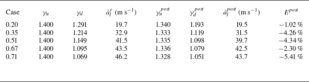
Richtmyer–Meshkov instability (Richtmyer Reference Richtmyer1960; Meshkov Reference Meshkov1969), commonly known as RMI, is a canonical hydrodynamic instability that arises when a perturbed interface separating two fluids of different densities is impulsively accelerated by a shock wave. It is of fundamental importance in various engineering applications and natural phenomena (Zhou Reference Zhou2017a
,
Reference Zhoub
, Reference Zhou2024; Zhou et al. Reference Zhou, Clark, Clark, Glendinning, Skinner, Huntington, Hurricane, Dimits and Remington2019, Reference Zhou2021), including inertial confinement fusion (ICF) (Zhou, Sadler & Hurricane Reference Zhou, Sadler and Hurricane2025), scramjet (Seleznev, Surzhikov & Shang Reference Seleznev, Surzhikov and Shang2019), and supernova explosion (Abarzhi et al. Reference Abarzhi, Bhowmick, Naveh, Pandian, Swisher, Stellingwerf and Arnett2019). In ICF, RMI is induced when strong shock waves triggered by laser or X-ray interact with the interfaces of the capsule, leading to undesired mixing between external ablative material and internal fuel, thereby reducing the energy gain. The effect of hydrodynamic instabilities on ICF implosion is strongly dependent on the design of the target (Zhou et al. Reference Zhou, Sadler and Hurricane2025). The target has a variety of types, such as conventional single-shell capsules and advanced double-shell capsules. The former features a simpler structure, whereas the latter provides a broader design space due to the flexibility of potential materials for the outer and inner shells (Montgomery et al. Reference Montgomery2018; Kritcher et al. Reference Kritcher2022). Furthermore, to improve the stability of the fuel–capsule interface and narrow the imploding shell profile, it was proposed to dope the materials of the inner layers with high-Z material (Berzak Hopkins et al. Reference Berzak Hopkins2018; Peterson, Johnson & Haan Reference Peterson, Johnson and Haan2018). These suggest that different interfaces within various types of targets may have significantly different Atwood numbers, defined as
 $A_t=(\rho _d - \rho _u)/(\rho _d + \rho _u)$
, where
 $\rho _u$
and
 $\rho _d$
represent the densities of substances upstream and downstream of the interface, respectively. Therefore, understanding the dependence of RMI on
 $A_t$
is of great significance.
For RMI induced by a weak shock wave (weak-shock RMI), the perturbation evolution can be considered to initially undergo a linear compressible stage, followed by a nonlinear incompressible stage (Zhang & Sohn Reference Zhang and Sohn1997). Theoretically, Richtmyer (Reference Richtmyer1960) proposed an impulsive model, which treats RMI as a limiting case of the Rayleigh–Taylor instability (Rayleigh Reference Rayleigh1882; Taylor Reference Taylor1950) driven by an instantaneous rather than a constant acceleration, to predict the linear amplitude growth rate (
 $\dot {a}_l$
) of a light–heavy interface. This model accounts for compressibility effects in an empirical manner by employing post-shock Atwood number and amplitude (
 $A_t^1$
and
 $a_1$
), instead of their pre-shock values (
 $A_t^0$
and
 $a_0$
), for prediction. For the heavy–light interface configurations, Meyer & Blewett (Reference Meyer and Blewett1972) found that substituting
 $a_1$
with the average of
 $a_0$
and
 $a_1$
in the impulsive model yields improved agreement with their numerical results. By considering the temporal variations of the perturbation amplitude and
 $A_t$
during the shock–interface interaction, and combining the expressions of Richtmyer (Reference Richtmyer1960) and Meyer & Blewett (Reference Meyer and Blewett1972), Vandenboomgaerde, Gauthier & Mügler (Reference Vandenboomgaerde, Gauthier and Mügler2002) developed a refined formulation. For ideal-gas configurations, these heuristic prescriptions yield reasonably accurate predictions for weak shocks and/or high specific heat ratios, where compressibility effects are negligible (Velikovich, Herrmann & Abarzhi Reference Velikovich, Herrmann and Abarzhi2014). However, their predictive accuracy across diverse parameter regimes remains uncertain. This limitation stems from the absence of a derivation grounded in first principles, as well as the neglect of the full acoustic coupling history (Napieralski et al. Reference Napieralski, Cobos, Velikovich and Huete2024). Consequently, these prescriptions are insufficient for providing a general description of compressible linear RMI. Beyond the impulsive model, Richtmyer (Reference Richtmyer1960) incorporated the full acoustic coupling history through derivation of the fundamental governing equations, and proposed a compressible linear theory (Richtmyer theory) that predicts the linear evolution of a light–heavy interface under arbitrary compressibility conditions. Building on the work of Richtmyer (Reference Richtmyer1960), Yang, Zhang & Sharp (Reference Yang, Zhang and Sharp1994) derived a compressible linear theory for the heavy–light interface scenarios. Moreover, Wouchuk (Reference Wouchuk2001a
,
Reference Wouchukb
) derived exact compressible linear theories that are applicable to arbitrary shock intensities, fluid compressibilities and interface density ratios. Recently, Napieralski et al. (Reference Napieralski, Cobos, Velikovich and Huete2024) proposed an analytical, fully compressible theory for RMI involving reflected shocks with arbitrary equations of state. The principal advances lie in employing the inverse Laplace transform to solve the initial-value perturbation problem, and in extending previous theories beyond restrictions to specific equations of state. As the interface further evolves and pressure perturbations near the interface diminish, compressibility weakens and nonlinearity begins to dominate, marking the transition to the incompressible nonlinear stage. Based on this concept, several empirical nonlinear models (Zhang & Sohn Reference Zhang and Sohn1997; Sadot et al. Reference Sadot, Erez, Alon, Oron, Levin, Erez, Ben-Dor and Shvarts1998; Mikaelian Reference Mikaelian2003; Dimonte & Ramaprabhu Reference Dimonte and Ramaprabhu2010; Zhang & Guo Reference Zhang and Guo2016, Reference Zhang and Guo2022) were developed by appropriately matching the compressible linear and incompressible nonlinear solutions, all of which incorporate terms describing the influence of
 $A_t^0$
on the nonlinear evolution law. Notably, the simplified two-period division of RMI evolution employed in constructing existing nonlinear models may not apply to strong-shock scenarios, as compressibility may persist significantly even in strongly nonlinear stages.
Experimentally, RMI has been extensively investigated across a wide range of
 $A_t^0$
(Zhou Reference Zhou2024), primarily under weak-shock conditions with shock Mach number (
 $M$
) below 1.5. Using various gas combinations across interfaces formed by nitrocellulose membranes, Meshkov (Reference Meshkov1969) conducted experiments on weak-shock RMI over a range of
 $A_t^0$
. The experimental
 $\dot {a}_l$
(
 $\dot {a}_l^e$
) was found to be significantly lower than the prediction of the impulsive model (
 $\dot {a}_l^i$
), possibly due to nonlinear effects and the influence of the membrane support structure. Using methods similar to those employed by Meshkov (Reference Meshkov1969), Yosef-Hai et al. (Reference Yosef-Hai, Sadot, Kartoon, Oron, Levin, Sarid, Elbaz, Ben-Dor and Shvarts2003) investigated the late-time growth of weak-shock RMI with
 $A_t^0 \approx 0.19$
and 0.67. The predictions of the SEA model (Sadot et al. Reference Sadot, Erez, Alon, Oron, Levin, Erez, Ben-Dor and Shvarts1998) were found to align closely with the experimental results. Moreover, a comparison between scenarios with low and high
 $A_t^0$
shows that the spike evolution exhibits a stronger dependence on
 $A_t^0$
compared to the bubble growth. Mariani et al. (Reference Mariani, Vandenboomgaerde, Jourdan, Souffland and Houas2008) utilised stereolithography to fabricate the membrane supports, and on this basis generated gaseous interfaces with
 $A_t^0 \approx -0.76$
and 0.67. Laser-sheet diagnostics were employed to visualise the interface evolution. For the heavy–light interface scenario, a favourable agreement is reached between the experimental and theoretical/numerical results. In contrast, for the light–heavy interface scenario, significant deviations were observed between experimental data and theoretical/numerical counterparts, probably due to the influence of membrane fragments.
To avoid the influence of support structure and membrane fragments on instability evolution, Jacobs & Sheeley (Reference Jacobs and Sheeley1996) proposed a membraneless interface formation method utilising gravitational stratification. Based on this approach, they experimentally investigated the weak-shock RMI in a two-liquid system, considering
 $A_t^0$
ranging from 0.14 to 0.30. A fixed coil spring was employed to impart vertical acceleration to the test tank containing stratified liquids, thereby initiating the instability. Discrepancies between
 $\dot {a}_l^e$
and theoretical predictions were found and attributed to the finite bounce length. Subsequently, Collins & Jacobs (Reference Collins and Jacobs2002) generated continuous gaseous interfaces using the membraneless method, and investigated the development of weak-shock RMI with
 $A_t^0 \approx 0.60$
. By incorporating the diffuse-interface correction factor, a reasonable agreement between
 $\dot {a}_l^e$
and
 $\dot {a}_l^i$
was reached. Additionally, the nonlinear evolution data exhibit a reasonable agreement with the predictions of the ZS model (Zhang & Sohn Reference Zhang and Sohn1997) and SEA model. Later, Niederhaus & Jacobs (Reference Niederhaus and Jacobs2003) experimentally investigated weak-shock RMI on a membraneless liquid interface with
 $A_t^0 \approx -0.16$
. High-resolution planar laser-induced fluorescence imaging provided a clear visualisation of the interface, and the linear theoretical prediction was found to agree excellently with the experimental results.
Recently, by using the soap-film technique and gas-layer scheme to produce well-defined initial interfaces with various gas combinations, weak-shock RMI with
 $A_t^0$
ranging from
 $-0.94$
to 0.84 was investigated via shock-tube experiments (Chen et al. Reference Chen, Xing, Wang, Zhai and Luo2023; Xing et al. Reference Xing, Chen, Li, Wang, Zhai and Luo2025). For the light–heavy interface scenario, the impulsive model yields favourable predictions for
 $\dot {a}_l^e$
over a wide
 $A_t^0$
range. In contrast, for the heavy–light interface scenario, the models proposed by Li et al. (Reference Li, Chen, Zhai and Luo2024) and Wouchuk & Nishihara (Reference Wouchuk and Nishihara1997) effectively describe the start-up and linear stages, respectively, under diverse
 $A_t^0$
conditions. Moreover, none of the considered nonlinear models (Zhang & Sohn Reference Zhang and Sohn1997; Sadot et al. Reference Sadot, Erez, Alon, Oron, Levin, Erez, Ben-Dor and Shvarts1998; Mikaelian Reference Mikaelian2003; Dimonte & Ramaprabhu Reference Dimonte and Ramaprabhu2010; Zhang & Guo Reference Zhang and Guo2016, Reference Zhang and Guo2022) can accurately describe the interface evolution across all considered
 $A_t^0$
conditions, and their predictive capabilities were analysed and summarised. On this basis, a modified model applied to predict the weakly nonlinear evolution of weak-shock RMI with
 $A_t^0$
ranging from
 $-0.94$
to
 $-0.27$
, and from 0.24 to 0.84, was proposed.
At present, the Atwood-number dependence of weak-shock RMI has been well understood through experiments. However, high-intensity shocks are commonly encountered in practical RMI-related applications such as ICF. Therefore, investigating the RMI driven by a strong shock wave, referred to as strong-shock RMI, across a wide range of
 $A_t^0$
conditions is highly desirable. Laser-driven experiments on strong-shock RMI have been extensively conducted (Zhou Reference Zhou2017a
,
Reference Zhoub
; Zhou et al. Reference Zhou, Sadler and Hurricane2025). However, the perturbation evolution in these experiments would be influenced by additional physicochemical processes, such as material phase transition and plasma diffusion, making it challenging to isolate the contribution of RMI to the perturbation growth. In addition to laser-driven experiments, only a few shock-tube experiments on strong-shock RMI with
 $M \gt 2.0$
have been conducted, primarily due to the difficulty in generating a controllable strong shock in a shock-tube facility. In particular, only one known shock-tube experimental study has covered a range of
 $A_t^0$
values under strong-shock conditions (Motl et al. Reference Motl, Oakley, Ranjan, Weber, Anderson and Bonazza2009). Motl et al. (Reference Motl, Oakley, Ranjan, Weber, Anderson and Bonazza2009) investigated the evolution of membraneless interfaces accelerated by shock waves with
 $M$
up to 2.86, considering
 $A_t^0$
ranging from 0.29 to 0.95. The interface was observed to deviate more rapidly from a symmetric configuration under conditions of higher
 $M$
and
 $A_t^0$
. Moreover,
 $\dot {a}_l^e$
was found to be generally lower than
 $\dot {a}_l^i$
, which was attributed to the influence of the undesired diffusion layer.
Overall, desirable and systematic experimental research on the Atwood-number dependence of strong-shock RMI remains scarce. The underlying evolution mechanisms of strong-shock RMI under various
 $A_t^0$
conditions, along with the applicability of existing models, remain inadequately understood, thereby motivating the present study. In our recent work (Jiang et al. Reference Jiang, Cai, Xie, He, Wang, Si and Luo2024), a shock-tube facility capable of producing planar shocks with
 $M \gt 3.0$
while maintaining a ‘clean’ experimental flow was developed. Furthermore, a novel technique enabling the controllable generation of interfaces without support structure and diffusion layer was proposed. These advancements provide a rare opportunity to investigate the Atwood-number dependence of strong-shock RMI. In this study, experiments on strong-shock RMI with low, moderate and high
 $A_t^0$
are first conducted using the newly developed facility and technique. Next, the interface evolution features under diverse
 $A_t^0$
conditions are discussed. Finally, the dependence of linear, nonlinear and modal evolutions on
 $A_t^0$
is explored, and the predictive capabilities of existing models are evaluated.
2. Experimental methods
Experimental investigation of RMI has three fundamental elements: the shock wave, the initial interface, and flow diagnostics. Given the high sensitivity of RMI to initial conditions (Zhou Reference Zhou2017a , Reference Zhoub ), the controllable generation of both the shock wave and initial interface is critical. Equally important, flow diagnostics determine the extent to which the effective experimental information can be accurately captured.
To achieve a controllable generation of strong shock waves with
 $M \gt 3.0$
while maintaining a ‘clean’ post-shock flow, a novel shock-tube facility, as sketched in figure 1(a), was developed (Jiang et al. Reference Jiang, Cai, Xie, He, Wang, Si and Luo2024). The underlying working principle of this facility is that the shock intensity increases as the shock area decreases (Chester Reference Chester1954; Chisnell Reference Chisnell1957; Whitham Reference Whitham1957). The reduction in shock area is achieved through a convergence section specifically designed based on the geometrical shock dynamics theory (Han & Yin Reference Han and Yin1993), which enables a smooth shock convergence while minimising post-shock flow perturbations. During the convergence process, the cross-sectional area of the shock wave varies from 120 mm
 $\times$
262 to 120 mm
 $\times$
8 mm, leading to an increase in
 $M$
from approximately 2.0 to higher than 3.0. Further details on this facility are available in our previous work (Jiang et al. Reference Jiang, Cai, Xie, He, Wang, Si and Luo2024).
Sketches of (a) the shock-tube facility, (b) the interface formation process, and (c) the high-speed shadowgraph system.

To generate long-lasting discontinuous interfaces with minimal influence on the flow evolution, the polyester-film technique developed specifically for strong-shock experiments (Jiang et al. Reference Jiang, Cai, Xie, He, Wang, Si and Luo2024) is employed. The interface formation devices (A and B), as illustrated in figure 1(b), are manufactured by assembling transparent acrylic plates and pedestals, with adjacent boundaries machined into the profile of the initial interface. Polyester films of thickness 2
 $\unicode{x03BC}$
m are carefully attached to the upstream and downstream sides of device B using double-sided tape. The low height of the experimental flow field (8 mm) ensures that the polyester film can be well constrained by the upper and lower boundaries, thus eliminating the need for support structures. Moreover, the polyester film has a negligible influence on the flow visualisation, as it undergoes instantaneous pyrolysis and combustion in the high-temperature, oxygen-rich post-shock environment. Specifically, according to Martín-Gullón et al. (Reference Martín-Gullón, Esperanza and Font2001), polyester film begins to melt at approximately 525 K, and starts to decompose at approximately 650 K. The decomposition rate increases markedly at approximately 750 K, and complete decomposition occurs at approximately 1050 K. In the present experiments, the temperature of the gas upstream of the post-shock polyester film can reach up to 1000 K. Moreover, since the upstream gas is pure air (see below), the polyester film can be considered effectively exposed to an oxygen-rich environment, even though the oxygen concentration of the downstream gas varies across experiments. In light of the previous research by Martín-Gullón et al. (Reference Martín-Gullón, Esperanza and Font2001), the polyester film is expected to undergo near-complete pyrolysis and combustion under the present experimental conditions. To further substantiate this point, we provide in Appendix A a comparative analysis with a previous experiment using the same shock tube and interface-formation technique, but employing a different gas combination at the interface (air–He). This comparison provides indirect yet compelling evidence supporting the complete combustion of polyester in the present experiments. To achieve a wider variation of
 $A_t^0$
, it is desirable to replace the air on both sides of the polyester film with various types of gases, which can be achieved via the gas-layer scheme (Chen et al. Reference Chen, Xing, Wang, Zhai and Luo2023; Xing et al. Reference Xing, Chen, Li, Wang, Zhai and Luo2025). However, this scheme is not applicable in the current experiments due to the shock-proximity phenomenon: under strong-shock conditions, the shocked interface tends to remain close to the transmitted shock for an extended period. In such cases, the auxiliary interface in the gas-layer scheme may be too close to the target interface, thereby affecting the latter’s evolution through interfacial coupling. Therefore, in this study, the upstream gas remains air, and
 $A_t^0$
is adjusted by varying the composition of the downstream gas. Candidate downstream heavy gases include
 ${\textrm{CO}}_2$
,
 ${\textrm{SF}}_6$
and
 ${\textrm{C}}_4{\textrm{F}}_{10}$
.
The flow evolution is visualised using a high-speed shadowgraph system as depicted in figure 1(c). The system consists of a light source (CEL-PF300-T10), a slit for shaping the emitted light, an optical lens to collimate the beam, two concave mirrors (400 mm in diameter) for converting between spherical and parallel beams, two planar mirrors to guide the light vertically through the test section, and a high-speed video camera (Phantom V2012). In comparison with the schlieren imaging technique widely employed in conventional shock-tube experiments on RMI, the shadowgraph imaging method offers superior image contrast and enhanced feature discernibility in the presence of strong pressure perturbations near the interface. The frame rate of the camera is set to 100 000 frames per second, with exposure time 1
 $\unicode{x03BC}$
s. The spatial resolution of the shadowgraphs is approximately 0.57 mm pixel
 $^{-1}$
.
Five experiments on strong-shock RMI at single-mode light–heavy interfaces with different
 $A_t^0$
, hereafter referred to as cases
 $A_t^0$
, are performed. It is noted that the results of case 0.67 were reported in our previous work (Si et al. Reference Si, Jiang, Cai, Wang and Luo2025). The perturbation wavelength and scaled initial amplitude (
 $ka_0$
, where
 $k$
represents perturbation wavenumber) are fixed at 40.00 mm and 0.314, respectively. The key parameters for the five experiments are summarised in table 1. To evaluate the experimental reliability, Appendix B presents a comprehensive discussion of the uncertainties associated with shock and interface velocities, shadowgraph timing, gas component, and amplitude extraction. These analyses indicate that the experimental uncertainties remain minimal, and the present experiments are reliable. Moreover, although variations in
 $M$
exist across the experiments, as detailed in Appendix C, this does not undermine the robustness of the comparative analyses across the different cases. Furthermore, as previously reported (Si et al. Reference Si, Jiang, Cai, Wang and Luo2025), the maximum thickness of the boundary layer in the interface region remains significantly smaller than the cross-sectional width and height of the experimental flow field. Accordingly, the boundary layer has a negligible influence on the interface evolution.
Key parameters for five experimental cases labelled by pre-shock Atwood number (
 $A_t^0$
):
 $T$
is ambient temperature,
 $A_t^1$
is post-shock Atwood number,
 $M$
is incident shock Mach number,
 $v^e_{\textit{is}}$
and
 $v^e_{\textit{ts}}$
are experimental velocities of the incident and transmitted shocks, respectively,
 $u^e_{\textit{si}}$
and
 $u^t_{si}$
are velocities of the shocked interface obtained from experiments and predicted by one-dimensional gas dynamics theory, respectively, and
 $\gamma _d$
is specific heat ratio of downstream gas. The units of temperature and velocity are K and m
 ${\textrm{s}}^{-1}$
, respectively.

Among the three heavy gases employed,
 ${\textrm{C}}_4{\textrm{F}}_{10}$
possesses the lowest thermal stability. We therefore provide a brief analysis of its thermodynamic behaviour under post-shock conditions. According to the study by Yu et al. (Reference Yu, Kennedy, Ong, Mackie, Han and Dlugogorski2008), the lower temperature threshold for the pyrolysis of
 ${\textrm{C}}_4{\textrm{F}}_{10}$
is approximately 873 K, at which the concentration of the products approaches the detection limit. Therefore,
 ${\textrm{C}}_4{\textrm{F}}_{10}$
can be considered thermally stable below 873 K. In the current experiments, the post-shock temperature of
 ${\textrm{C}}_4{\textrm{F}}_{10}$
is approximately 545 K, which is safely below the threshold for thermal decomposition. Moreover, the total mass of the membrane is merely
 $\sim{\kern-1.5pt}2.6$
mg, and the experiment lasts only
 $\sim{\kern-1.5pt}350$
 $\unicode{x03BC}$
s. Consequently, even though the flame temperature during polyester combustion can exceed 700 K, as reported in the literature (Hilado Reference Hilado1998), the limited heat release and short duration prevent a significant increase in the bulk
 ${\textrm{C}}_4{\textrm{F}}_{10}$
temperature. As a result, no ignition or thermal decomposition of
 ${\textrm{C}}_4{\textrm{F}}_{10}$
is anticipated. Moreover, the elevated post-shock temperature is high enough to excite molecular vibrational excitation in the experimental gases (e.g. air, CO
 $_2$
, SF
 $_6$
and
 ${\textrm{C}}_4{\textrm{F}}_{10}$
), leading to variations in the specific heat ratio
 $\gamma$
. Nevertheless, as discussed in Appendix D, this variation exerts a negligible influence on the interface evolution.
3. Flow features under diverse Atwood-number conditions
Experimental shadowgraphs illustrating the evolution of strong-shock RMI at single-mode light–heavy interfaces with various
 $A_t^0$
are presented in figure 2. To provide a more comprehensive illustration of the interface dynamics, movies showing all five experiments are included in the supplementary material. These movies capture the full temporal evolution of strong-shock RMI under diverse
 $A_t^0$
conditions, providing a continuous representation that complements the static snapshots presented in figure 2. Waves travelling at velocities substantially exceeding that of the incident shock are generally observed in the videos after the shock–interface interaction. Notably, these waves do not represent conventional pressure perturbations in the flow field, but instead correspond to strain waves transmitted through the acrylic interface-generation apparatus. Their presence is attributed to the inevitable small gaps between the apparatus and the shock tube, together with the abrupt pressure fluctuations induced by the strong shock.
Experimental shadowgraphs of the evolution of strong-shock RMI at single-mode light–heavy interfaces with various
 $A_t^0$
. Numbers represent time in
 $\unicode{x03BC}$
s.

The temporal origin (
 $t = 0$
 $\unicode{x03BC}$
s) in the experimental shadowgraphs corresponds to the moment when the incident shock reaches the mean position of the initial interface. Additionally, after the shock–interface interaction, the shadows caused by the connection edges of the interface formation devices, which do not provide additional information on the flow evolution, are removed from the images through post-processing to enhance visual clarity. Case 0.35 is selected as a representative example to illustrate the overall flow evolution process. When the incident shock interacts with the initial interface, a transmitted shock and a reflected shock are generated. The reflected shock also propagates downstream as the flow Mach number of the region ahead (1.45) exceeds its own Mach number (1.14). Meanwhile, the shocked interface starts to evolve under the drive of baroclinic vorticity and pressure perturbations. The shocked interface initially maintains a single-mode morphology (26
 $\unicode{x03BC}$
s), and gradually becomes asymmetric (116
 $\unicode{x03BC}$
s) due to the generation of higher-order modes. Subsequently, distinct spike and bubble structures emerge (206
 $\unicode{x03BC}$
s). Before the interface exits the observation window, no discernible roll-up structure forms at the spike.
A comparison of the shadowgraphs for experiments with various
 $A_t^0$
reveals that the nonlinear evolution features of the shocked interface, including spike, bubble and roll-up structures, emerge earlier and evolve more rapidly at higher
 $A_t^0$
. Specifically, in cases with relatively low
 $A_t^0$
(i.e. 0.20 and 0.35), the shocked interface maintains a quasi-single-mode profile until exiting the observation area. Moreover, the interface morphology resembles that under weak-shock conditions (Chen et al. Reference Chen, Xing, Wang, Zhai and Luo2023), although the bubble tip becomes appreciably flatter at late stages. For strong-shock RMI with moderate
 $A_t^0$
(i.e. case 0.51), the bubble front flattens progressively and approaches a planar configuration at later stages (200–270
 $\unicode{x03BC}$
s). Consequently, the interface exhibits a highly asymmetric profile and differs markedly from that under weak-shock conditions (Chen et al. Reference Chen, Xing, Wang, Zhai and Luo2023). This can be attributed to the more pronounced shock-proximity effect and the associated influence of transverse waves, propagating in the region between the transmitted shock and shocked interface, on interface evolution (i.e. the secondary-compression effect). The interface evolution in case 0.71 is broadly similar to that in case 0.67, which has been detailed in a prior study (Si et al. Reference Si, Jiang, Cai, Wang and Luo2025), though notable differences exist. Specifically, the spike becomes particularly sharp at early times (102
 $\unicode{x03BC}$
s), which should be attributed to the more pronounced spike-acceleration effect, i.e. high-order harmonics concentrate on the spike under high
 $A_t^0$
conditions, thereby promoting the evolution (Dimonte & Ramaprabhu Reference Dimonte and Ramaprabhu2010). Besides, the more significant shock-proximity and secondary-compression effects cause the bubble front to appear corrugated rather than flat. Moreover, strong transverse waves result in a highly disordered appearance of the region between the transmitted shock and the shocked interface in the shadowgraphs. Furthermore, the roll-up structures are more pronounced, leading to enhanced fluid mixing across the interface. Notably, the intense mixing of the gases renders the identification of vortices difficult. We therefore identify the roll-up structures based on another morphological feature, i.e. a broadened head accompanied by a slender neck (Zhou Reference Zhou2017a
,
Reference Zhoub
, Reference Zhou2024; Zhou et al. Reference Zhou, Clark, Clark, Glendinning, Skinner, Huntington, Hurricane, Dimits and Remington2019). Based on this criterion, the roll-up structure in case 0.71 is evident, with the head continuously broadening over time while the neck gradually narrows. In case 0.67, the roll-up structure appears less pronounced yet remains discernible within the overall interface evolution. By contrast, in cases with lower
 $A_t^0$
, such as case 0.51, the spike lacks the aforementioned morphological characteristics, indicating the absence of roll-up structures.
4. Linear, nonlinear and modal evolutions
4.1. Linear amplitude growth
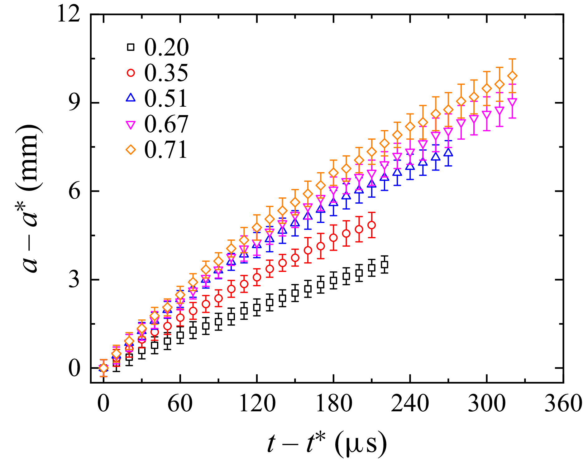
The temporal evolution of the dimensional overall interface amplitude (
 $a$
) for different cases is presented in figure 3. Here,
 $a$
is defined as half of the horizontal distance between the tips of the bubble and spike, and the determination of its uncertainty, represented by error bars, is presented in § B.4. Also,
 $t^*$
denotes the duration of the start-up period, i.e. a phase during which the amplitude growth rate rises from zero and gradually reaches
 $\dot {a}_l$
under the drive of pressure perturbations (Lombardini & Pullin Reference Lombardini and Pullin2009), and
 $a^*$
is the corresponding
 $a$
at
 $t = t^*$
. At early times,
 $a$
exhibits an approximately linear growth in all cases, and
 $\dot {a}_l^e$
is obtained by performing a linear fit to these data.
Temporal variations of perturbation amplitude in dimensional form for cases with different
 $A_t^0$
.

The classical impulsive model has been demonstrated to apply to weak-shock RMI at a small-amplitude single-mode light–heavy interface over a wide range of
 $A_t^0$
conditions, as reported by Chen et al. (Reference Chen, Xing, Wang, Zhai and Luo2023) (see table 2 herein). Notably, prior theoretical studies (Mikaelian Reference Mikaelian1994; Yang et al. Reference Yang, Zhang and Sharp1994; Velikovich et al. Reference Velikovich, Herrmann and Abarzhi2014) indicate that theoretically, the fundamental criterion for the model’s applicability is the low flow compressibility. This criterion not only remains valid for weak shocks, but can also hold at finite shock strengths, provided that
 $\gamma$
is sufficiently large. In the present study, the impulsive model is re-examined to evaluate the influence of strong flow compressibility arising from strong shocks and highly compressible fluids (
 ${\textrm{CO}}_2$
,
 ${\textrm{SF}}_6$
and
 ${\textrm{C}}_4{\textrm{F}}_{10}$
) on its applicability under diverse
 $A_t^0$
. It can be expressed as
 \begin{align} \dot {a}_l^i = ka_1 A_t^1 u^e_{si}. \end{align}
Here,
 $a_1=a_0(1 - u^e_{si}/v^e_{\textit{is}})$
, with
 $v^e_{\textit{is}}$
representing the experimentally measured velocity of the incident shock. Besides the semi-empirical impulsive model, it is particularly valuable to evaluate compressible linear theories (Richtmyer Reference Richtmyer1960; Wouchuk Reference Wouchuk2001a
; Napieralski et al. Reference Napieralski, Cobos, Velikovich and Huete2024), which are grounded in first principles and incorporate the full acoustic coupling history, as they provide a comprehensive description of compressible linear RMI. Notably, for conciseness, only the Richtmyer theory is considered here. Given the high similarity among the predictions of the compressible linear theories, the evaluation of the Richtmyer theory’s predictive capability can serve as a representative assessment of the others. The Richtmyer theory lacks an analytical solution and involves a set of nonlinear equations that need to be solved numerically. Details on this theory are available in the pioneering works of Richtmyer (Reference Richtmyer1960) and Yang et al. (Reference Yang, Zhang and Sharp1994).
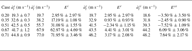
Comparison of experimental linear amplitude growth rate (
 $\dot {a}_l^e$
) with the predictions of the impulsive model (
 $\dot {a}_l^i$
), Richtmyer theory (
 $\dot {a}_l^r$
), and compressible impulsive model (
 $\dot {a}_l^{ci}$
). Here,
 $E^{i/r/ce}=(\dot {a}_{l}^{i/r/ci}-\dot {a}_{l}^{e})/\dot {a}_{l}^{e}$
is the relative error between
 $\dot {a}_{l}^{i/r/ci}$
and
 $\dot {a}_{l}^{e}$
.

Values of
 $\dot {a}_l^e$
,
 $\dot {a}_l^i$
, and
 $\dot {a}_l$
predicted by the Richtmyer theory (
 $\dot {a}_l^{r}$
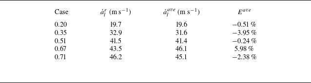
) for different cases are provided in table 2 for comparison. The relative error
 $E^{i/r}=(\dot {a}_{l}^{i/r}-\dot {a}_{l}^{e})/\dot {a}_{l}^{e}$
is introduced to quantify the deviation of
 $\dot {a}_{l}^{i/r}$
from
 $\dot {a}_{l}^{e}$
. The impulsive model provides an accurate prediction for case 0.20 (
 $E^{i}=2.95\,\%\pm2.97\,\%$
). However, for the other cases with higher
 $A_t^0$
, this model significantly overestimates
 $\dot {a}_l^e$
, and
 $E^{i}$
is larger at higher
 $A_t^0$
, reaching up to 71.95 %
 $\pm$
3.46 % for case 0.71. Compared with the observations of Chen et al. (Reference Chen, Xing, Wang, Zhai and Luo2023), the present findings demonstrate that flow compressibility induced by strong shocks and intrinsically compressible fluids exerts a significant influence on the predictive capability of the impulsive model, which is consistent with the theoretical predictions reported by Mikaelian (Reference Mikaelian1994), Yang et al. (Reference Yang, Zhang and Sharp1994) and Velikovich et al. (Reference Velikovich, Herrmann and Abarzhi2014). In contrast, the Richtmyer theory yields favourable predictions for all cases, with
 $|E^{r}|$
remaining below 7.50 %.
The above results indicate that the accuracy of the impulsive model is highly sensitive to
 $A_t^0$
. However, it is noteworthy that variations in the composition of the downstream gas influence not only the density but also
 $\gamma$
, a parameter characterising the gas compressibility. The
 $\gamma$
value of the gas upstream of the interface (
 $\gamma _u$
) is 1.40, while the
 $\gamma$
value of the gas downstream of the interface (
 $\gamma _d$
) varies across cases: 1.29, 1.21, 1.15, 1.09 and 1.07 for cases 0.20, 0.35, 0.51, 0.67 and 0.71, respectively. Quantitative evaluation of the effects of
 $A_t$
and
 $\gamma _d$
on the impulsive model’s accuracy necessitates a reliable benchmark, either experimental or theoretical, that ideally allows one parameter to vary while the other remains fixed. However, gas combinations satisfying the requirements may not exist naturally, posing challenges for establishing an experimental benchmark. Consequently, the Richtmyer theory is adopted as a theoretical benchmark in this study, and its validity under various initial conditions is further verified through numerical simulations, with details provided in Appendix E. To compare the predictions from the impulsive model and Richtmyer theory, three series of cases with the same
 $\gamma _u$
(1.40) but different
 $\gamma _d$
(1.29, 1.15 and 1.07) are considered. Note that 1.29, 1.15 and 1.07 correspond to
 $\gamma _d$
in cases 0.20, 0.51 and 0.71, respectively, and for clarity,
 $\gamma _d$
of cases 0.35 and 0.67 are not considered. Each case series includes five values of
 $A_t^0$
(0.20, 0.35, 0.51, 0.67 and 0.71), corresponding to five experiments.
To facilitate comparison, we follow the approach of Mikaelian (Reference Mikaelian1994) to normalise
 $\dot {a}_l$
as
 $\alpha_l=\dot{a}_l/ka_0u_{si}$
, where
 $u_{si}$
is the velocity of the shocked interface. The values of
 $\alpha _l$
predicted by the impulsive model (
 $\alpha _l^i$
) and Richtmyer theory (
 $\alpha _l^r$
) are plotted in figure 4 as functions of the shock intensity, which is defined as
 $\varepsilon = 1 - p_0/p_1$
, with
 $p_0$
and
 $p_1$
representing the pressures of gases in front of and behind the incident shock, respectively. Here,
 $\varepsilon$
ranges from 0 to 1, indicating shock intensities from extremely weak to extremely strong. When
 $\gamma _u$
and
 $\gamma _d$
are similar, as illustrated in figure 4(a),
 $\alpha _l^i$
and
 $\alpha _l^r$
are in reasonable agreement across a wide range of
 $A_t^0$
and
 $\varepsilon$
values. In contrast, when
 $\gamma _u$
and
 $\gamma _d$
differ significantly, as shown in figures 4(b) and 4(c),
 $\alpha _l^i$
increasingly deviates from
 $\alpha _l^r$
with increasing
 $\varepsilon$
. This discrepancy occurs at lower
 $\varepsilon$
and is more pronounced when the difference between
 $\gamma _u$
and
 $\gamma _d$
is greater and
 $A_t^0$
is higher. In other words, the predictive capability of the impulsive model is related to three key parameters governing the compressibility of the flow:
 $\gamma _u / \gamma _d$
,
 $\varepsilon$
and
 $A_t^0$
. The impulsive model yields accurate predictions when
 $\gamma _d$
is close to
 $\gamma _u$
, but its accuracy deteriorates at high
 $\varepsilon$
and
 $A_t^0$
when the disparity between
 $\gamma _d$
and
 $\gamma _u$
is significant.
Variations of dimensionless linear amplitude growth rate
 $\alpha _l$
with shock intensity
 $\varepsilon$
: theoretical predictions of the impulsive model and Richtmyer theory for the series of cases with
 $\gamma _d$
of (a) 1.29, (b) 1.15 and (c) 1.07.

The Richtmyer theory remains valid across both weak and strong compressibility regimes. However, its practical application is hindered by the need for tedious numerical computations. In contrast, the impulsive model offers simplicity and ease of use, but its accuracy deteriorates in highly compressible regimes. Therefore, developing a linear model that combines simplicity with robustness across a broad range of compressibility conditions is of considerable significance. Motivated by this need, we propose a modified impulsive model informed by experimental observations and theoretical predictions. The modified model, referred to as the compressible impulsive model, is formulated as
 \begin{align} \dot {a}_l^{ci} = \dot {a}_l^i \left \{\left [1-g\left (\frac {\gamma _u}{\gamma _d}\right )\right ] + g\left (\frac {\gamma _u}{\gamma _d}\right ) h(\varepsilon , A_t^0)\right \}\!, \end{align}
in which
 \begin{align} g\left (\frac {\gamma _u}{\gamma _d}\right ) = \frac {1}{1 + \textrm{e}^{-22\left (\frac {\gamma _u}{\gamma _d}-1.18\right )}} \quad \text{and} \quad h(\varepsilon , A_t^0) = \frac {1}{1+\left (\frac {6+8A_t^0}{1+15A_t^0}\right )\varepsilon ^{\frac {16+8A_t^0}{2+3A_t^0}}}. \end{align}
The ideas leading to such a model are elaborated as follows. A correction factor applied to
 $\dot {a}_l^i$
is introduced to account for the limitations of the impulsive model under varying compressibility conditions. This correction incorporates two primary functions, i.e.
 $g(\gamma _u / \gamma _d)$
and
 $h(\varepsilon , A_t^0)$
, that characterise the influence of three key parameters governing the compressibility of the flow:
 $\gamma _u / \gamma _d$
,
 $A_t^0$
and
 $\varepsilon$
. To preserve the high predictive accuracy of the impulsive model as
 $\gamma _u / \gamma _d$
approaches unity,
 $g(\gamma _u / \gamma _d)$
is constructed to vanish in this limit, thereby ensuring that
 $\dot {a}_l^{ci}$
reduces to
 $\dot {a}_l^i$
. Furthermore, to mitigate the increasing overprediction of
 $\dot {a}_l$
by the impulsive model as
 $\gamma _u / \gamma _d$
,
 $\varepsilon$
and
 $A_t^0$
increase,
 $h(\varepsilon , A_t^0)$
is defined to remain below unity and to decrease monotonically with increasing
 $\varepsilon$
and
 $A_t^0$
, while
 $g(\gamma _u / \gamma _d)$
is designed to increase and approach unity as
 $\gamma _u / \gamma _d$
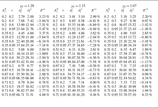
increases. The comparison between
 $\dot {a}_{l}^{e}$
(
 $\dot {a}_l^{r}$
) and
 $\dot {a}_{l}^{ci}$
is presented in table 2 (table 3), in which
 $E^{ce}=(\dot {a}_{l}^{ci}-\dot {a}_{l}^{e})/\dot {a}_{l}^{e}$
(
 $E^{cr}=(\dot {a}_{l}^{ci}-\dot {a}_{l}^{r})/\dot {a}_{l}^{r}$
) denotes the relative error between
 $\dot {a}_{l}^{ci}$
and
 $\dot {a}_{l}^{e}$
(
 $\dot {a}_{l}^{r}$
). It is observed that
 $E^{ce}$
and
 $E^{cr}$
remain below 10 %, indicating that the compressible impulsive model maintains high predictive accuracy across a broad range of flow compressibility conditions.
Comparison of
 $\dot {a}_l$
predicted by the Richtmyer theory and the compressible impulsive model (
 $\dot {a}_l^r$
and
 $\dot {a}_{l}^{ci}$
). Here,
 $E^{cr}=(\dot {a}_{l}^{ci}-\dot {a}_l^r)/\dot {a}_l^r$
is the relative error between
 $\dot {a}_l^r$
and
 $\dot {a}_{l}^{ci}$
. Units of
 $\dot {a}_l^r$
and
 $\dot {a}_{l}^{ci}$
are m
 ${\textrm{s}}^{-1}$
.

Notably, although the compressible impulsive model is indeed simpler and computationally more efficient than the Richtmyer theory, given present computational capabilities, the runtime difference does not constitute a principal advantage. Instead, its principal merit over the Richtmyer theory, deriving predictions by solving a set of nonlinear equations numerically, lies in its explicit formulation, which establishes clear and explicit relationships between model predictions and key physical parameters, such as
 $ka_0$
,
 $\gamma _u / \gamma _d$
,
 $A_t^0$
and
 $\varepsilon$
. In other words, although the compressible impulsive model, a heuristic prescription, cannot be deemed sufficient for a comprehensive description of compressible linear RMI as it neglects the complete history of acoustic coupling, its simplicity facilitates a clearer understanding of the dependence of linear evolution on the initial conditions.
Temporal variations of perturbation amplitude in dimensionless form for (a,b) case 0.20, (c,d) case 0.51, and (e,f) case 0.71: (a, c, e) overall interface; (b, d, f) bubble and spike.

4.2. Nonlinear amplitude evolution
As the interface enters the nonlinear evolution period, its profile becomes distinctly asymmetric, and the bubble and spike exhibit markedly different evolutionary behaviours. The determination of the amplitudes of the bubble and spike (
 $a_b$
and
 $a_s$
) and their associated uncertainties is described in detail in § B.4. The temporal variations of
 $a$
and
 $a_{b/s}$
in dimensionless form are illustrated in figure 5. Here,
 $t$
,
 $a$
and
 $a_{b/s}$
are non-dimensionalised as
 $\tau=k \dot {a}_{l}^{e}(t - t^*)$
,
 $\alpha=k(a - a^*)$
and
 $\alpha_{b/s}=k(a_{b/s} - a^*_{b/s})$
, respectively, in which
 $a^*_{b/s}$
denotes the value of
 $a_{b/s}$
at
 $t = t^*$
. Representative nonlinear models, including the ZS, SEA, MIK (Mikaelian Reference Mikaelian1994), DR (Dimonte & Ramaprabhu Reference Dimonte and Ramaprabhu2010), ZG (Zhang & Guo Reference Zhang and Guo2016) and ZG-new (Zhang & Guo Reference Zhang and Guo2022) models, are considered for evaluation, with detailed expressions available in our previous work (Chen et al. Reference Chen, Xing, Wang, Zhai and Luo2023). A comparison between experimental and theoretical results reveals that the predictive performance of these models for cases 0.35 and 0.67 closely resembles that for cases 0.20 and 0.71, respectively. For clarity, three experimental cases (cases 0.20, 0.51 and 0.71), representing strong-shock RMI with low, moderate and high
 $A_t^0$
, respectively, are chosen for detailed discussion. Notably, the nonlinear models initialised using
 $\dot {a}_{l}$
can be regarded as effectively incompressible, since
 $\dot {a}_{l}$
describes the dominant early-time compressibility effects (Dimonte & Ramaprabhu Reference Dimonte and Ramaprabhu2010), i.e. continuous pressure perturbations induced by disturbed transmitted and reflected waves. Thus these models, together with the systematic analyses of their predictive capabilities concerning weak-shock RMI over a broad range of
 $A_t^0$
reported by Chen et al. (Reference Chen, Xing, Wang, Zhai and Luo2023) (see figure 5 herein), constitute essential references for evaluating the influence of compressibility on nonlinear evolution dynamics.
For strong-shock RMI with low
 $A_t^0$
, all models yield reasonable predictions for the overall interface growth, as well as the individual evolution of the bubble and spike, which closely resembles the behaviour observed in the weak-shock RMI scenario (Chen et al. Reference Chen, Xing, Wang, Zhai and Luo2023). This finding highlights that the influence of compressibility effects, specifically shock proximity and secondary compression, is rather limited under such conditions, which can primarily be ascribed to the thermodynamic properties of the downstream gas, i.e.
 ${\textrm{CO}}_2$
. Its relatively large
 $\gamma$
and low molecular mass lead to a rapid separation of the transmitted shock from the interface. As a result, the shock-proximity effect and the associated secondary-compression effect remain weak, and accordingly, the predictive performance of the models is similar to that under weak-shock conditions (Chen et al. Reference Chen, Xing, Wang, Zhai and Luo2023).
For strong-shock RMI with moderate
 $A_t^0$
, the predictive performance of the models differs substantially from that under weak-shock conditions (Chen et al. Reference Chen, Xing, Wang, Zhai and Luo2023). This indicates that the increase in
 $M$
introduces additional physical mechanisms that alter the nonlinear evolution dynamics. For the bubble, these models, which have been validated under weak-shock conditions (Chen et al. Reference Chen, Xing, Wang, Zhai and Luo2023), underestimate the amplitude growth. This can be attributed to the fact that the shock-proximity and secondary-compression effects are significant in this scenario, yet they are not accounted for in these models. For the spike, the experimental results exhibit favourable agreement with the predictions of the ZS, DR and ZG-new models, but fall below the SEA model prediction, and above those of the MIK and ZG models. It is noteworthy that in the weak-shock RMI, the spike growth agrees well with the predictions of the MIK and ZG models that do not consider the spike-acceleration effect (Chen et al. Reference Chen, Xing, Wang, Zhai and Luo2023), suggesting that this effect is negligible or rather weak at moderate
 $A_t^0$
. The promotion of spike growth relative to weak-shock RMI can be attributed to the significant shock-proximity phenomenon, wherein the high-pressure region generated by the transmitted shock persists near the spike root for an extended duration, thereby accelerating the spike evolution. Consequently, the observed favourable prediction of the ZS, DR and ZG-new models for the experimental data is accidental: their overestimation of the spike-acceleration effect coincidentally describes the shock-proximity effect on spike growth. The MIK and ZG models, which have not considered the shock-proximity effect on spike growth, underestimate the spike evolution. In contrast, the SEA model still overestimates the spike evolution, owing to its excessive overestimation of the spike-acceleration effect (Dimonte & Ramaprabhu Reference Dimonte and Ramaprabhu2010; Chen et al. Reference Chen, Xing, Wang, Zhai and Luo2023; Xing et al. Reference Xing, Chen, Li, Wang, Zhai and Luo2025).
For strong-shock RMI with high
 $A_t^0$
, a pronounced spike-acceleration effect is observed: the spike sustains a high growth rate throughout the experiment, causing the overall interface amplitude to seemingly exhibit weakly nonlinear growth, despite the interface having already entered a strongly nonlinear regime. For the bubble, as in the moderate
 $A_t^0$
scenario, amplitude growth is suppressed by shock-proximity and secondary-compression effects, leading models that are valid under weak-shock conditions (Chen et al. Reference Chen, Xing, Wang, Zhai and Luo2023) to underestimate the growth. For the spike, the ZS, DR and ZG-new models that capture the spike-acceleration effect and perform well under weak-shock conditions (Chen et al. Reference Chen, Xing, Wang, Zhai and Luo2023) also provide a reasonable prediction under strong-shock conditions, with only slight underestimation overall. This indicates that although the shock-proximity effect enhances spike growth, its influence is minor relative to the spike-acceleration effect, and thus does not fundamentally affect the predictive performance of the models. Moreover, the MIK and ZG models, which do not consider both spike-acceleration and shock-proximity effects, underestimate spike growth, whereas the SEA model overestimates it due to excessive prediction of the spike-acceleration effect.
Summarising the above analysis, under low-
 $A_t^0$
conditions, the shock-proximity phenomenon is not significant. As a result, the compressible effects on interface evolution are weak, and the evolution can be reasonably described by existing models. As
 $A_t^0$
increases to moderate and high magnitudes, the shock-proximity phenomenon becomes pronounced, and compressible effects significantly suppress the bubble growth. Additionally, the spike-acceleration and shock-proximity effects appear and promote the spike evolution. For the spike growth, the ZS, DR and ZG-new models yield reasonable predictions across all cases, whether physical or incidental. However, none of the existing models can accurately predict the bubble evolution under all
 $A_t^0$
conditions, as they do not consider compressibility effects that persist into the nonlinear phase.
A rigorous characterisation of the shock-proximity and secondary-compression effects under varying
 $A_t^0$
conditions is highly challenging. Thus we attempt to propose an empirical model for bubble evolution. The DR model not only captures the late-time
 $1/t$
behaviour of amplitude growth rate (Dimonte & Ramaprabhu Reference Dimonte and Ramaprabhu2010), but also offers an accurate description of bubble evolution across a broad range of
 $A_t^0$
under weak-shock conditions (Chen et al. Reference Chen, Xing, Wang, Zhai and Luo2023). Here, we extend the DR model by incorporating the compressibility effects introduced by strong shock waves. Based on the experimental results from the present work and a previous study (Chen et al. Reference Chen, Xing, Wang, Zhai and Luo2023), the modified DR model (J-DR model) is constructed as
 \begin{align} \begin{aligned} \dot {a}_{b}^{j-dr}= & N_{b}\dot {a}_l^{e} \frac {1+\left (1 - A_t^1\right ) N_{b}\tau }{1+C_{b} N_{b}\tau +\left (1 - A_t^1\right ) F_{b}(N_{b}\tau )^2}K_b, \\\text{in which} \ &\ C_{b}=[4.5 + A_t^1 + (2 - A_t^1) k a_1 ]/4, \quad F_{b}= 1 + A_t^1, \\& \ \ \ \ \ N_{b} = 1 - 0.6 \textrm{e}^{-8 \xi } - 0.05A_t^1(5-\xi ), \\K_b&=\frac {1}{1 + \textrm{e}^{3[\tau -f(\xi )]}} \quad \text{and} \quad f(\xi ) = 15 \xi ^2 + 1. \end{aligned} \end{align}
Notably, the expressions for
 $C_{b}$
and
 $F_{b}$
remain the same as those in the DR model. We next present the rationale behind the construction of the J-DR model.
To incorporate the shock-proximity effect, which primarily manifests in the early stage when the transmitted shock remains fairly close to the interface,
 $\dot {a}_l^{e}$
in the DR model is modified as
 $N_{b}\dot {a}_l^{e}$
, where
 $N_{b}$
is a coefficient with magnitude substantially less than unity. Experimental results indicate that the shock-proximity effect depends on two primary factors. The first factor is the degree of significance of the shock-proximity phenomenon, which can be quantified by
 $\xi=(v_{\textit{ts}}-u_{si})/u_{si}$
, where
 $v_{\textit{ts}}$
denotes the velocity of the transmitted shock. A smaller
 $\xi$
indicates a more pronounced shock-proximity phenomenon, and accordingly,
 $N_b$
is formulated as a monotonically increasing function of
 $\xi$
to reflect this trend. The second factor is the magnitude of
 $A_t^0$
: a higher
 $A_t^0$
leads to a slower early-time bubble growth. This phenomenon can be interpreted based on the following physical reasoning. The interface evolution is governed by the balance between fluid inertia and available kinetic energy. At higher
 $A_t^0$
, harmonics more rapidly transfer to the spike region, increasing the kinetic energy for spike growth (which is the intrinsic mechanism of the spike-acceleration effect), while reducing the kinetic energy available for bubble development. Meanwhile, the increased inertia contrast between the light and heavy fluids further reduces the ability of the light fluid to ‘push’ the heavy one. These result in slower bubble growth at higher
 $A_t^0$
conditions, and
 $N_b$
is accordingly formulated as a decreasing function of
 $A_t^1$
to capture this behaviour.
To capture the secondary-compression effect, which mainly manifests at a short period after the transverse shock interaction, a time-dependent function
 $K_b = 1/\{1+{\rm e}^{3[\tau -f(\xi )]}\}$
is incorporated into the model. Here,
 $f(\xi )$
represents the characteristic time at which transverse shock interaction occurs at the bubble tip;
 $K_b$
converges to 1 as
 $\tau - f(\xi ) \rightarrow -\infty$
, and to 0 as
 $\tau - f(\xi ) \rightarrow +\infty$
, with significant variation occurring only near
 $\tau = f(\xi )$
. In other words, at approximately
 $\tau = f(\xi )$
,
 $K_b$
rapidly transitions from approximately 1 to nearly 0, thus realising the description of the secondary-compression effect. The determination of
 $f(\xi )$
is informed by observations in prior RMI studies (Zhou Reference Zhou2017a
,
Reference Zhoub
, Reference Zhou2024) that the secondary-compression effect is negligible in the weak-shock limit, and the transverse wave intersection occurs earlier when the shock-proximity phenomenon is more pronounced. In other words,
 $f(\xi )$
is expected to tend to infinity as
 $\xi \rightarrow +\infty$
, and decrease as
 $\xi$
decreases. Taking into account the constraints imposed by these conditions as well as the experimental results,
 $f(\xi )$
is empirically determined as
 $15 \xi ^2 + 1$
. As illustrated in figure 5, the J-DR model yields accurate predictions for bubble evolution across a broad range of
 $A_t^0$
conditions.
4.3. Modal evolution
Modal analysis is conducted to investigate the modal evolution of strong-shock RMI under diverse
 $A_t^0$
conditions. For clarity, only cases 0.20, 0.51 and 0.71, representing strong-shock RMI with low, moderate and high
 $A_t^0$
, respectively, are considered for detailed analysis. The experimental modal information is extracted by identifying interface contours at stages preceding the appearance of roll-up structures, i.e. before the interface becomes multi-valued, and subsequently applying a fast Fourier transform. The modal models proposed by Zhang & Sohn (Reference Zhang and Sohn1997) (ZSM model) and Vandenboomgaerde et al. (Reference Vandenboomgaerde, Gauthier and Mügler2002) (VM model) are considered as theoretical references. Notably, both models were originally developed for incompressible flow conditions, thus their predictions, as well as their predictive performance for weak-shock RMI over a broad range of
 $A_t^0$
, reported by Chen et al. (Reference Chen, Xing, Wang, Zhai and Luo2023) (see figures 6 and 7 therein), provide valuable benchmarks for assessing the influence of compressibility on modal evolution. For the first three harmonics (
 $m_1$
,
 $m_2$
and
 $m_3$
), the temporal variations of their amplitudes (
 $a_{m1}$
,
 $a_{m2}$
and
 $a_{m3}$
) in dimensionless form, obtained from experiments and predicted by the ZSM and VM models, are presented in figures 6(a), 6(c) and 6(e). Additionally, to facilitate the understanding of the relationship between modal evolution and interface morphology, the modal characteristics of the shocked interface contours at
 $\tau \approx 0.55$
in cases 0.20, 0.51 and 0.71 are presented in figures 6(b), 6(d) and 6(f), respectively. Here,
 $a_{mi}$
(with
 $i=1,2,3$
) is normalised as
 $\alpha _{i}=k(a_{mi}-a_{mi}^*)$
, in which
 $a_{mi}^*$
denotes the corresponding
 $a_{mi}$
at
 $t=t^*$
.
(a,c,e) Modal evolutions obtained from experiments and predicted by ZSM and VM models, and (b,d,f) modal information on the contour of shocked interface at
 $\tau \approx 0.55$
for (a,b) case 0.20, (c,d) case 0.51, and (e,f) case 0.71. Here,
 $\alpha _1$
,
 $\alpha _2$
and
 $\alpha _3$
are dimensionless amplitudes of the first three harmonics
 $m_1$
,
 $m_2$
and
 $m_3$
, and SI means shocked interface.

For case 0.20, as shown in figure 6(a), the ZSM and VM models yield similar predictions, and both capture the evolution of
 $m_1$
with reasonable accuracy. Moreover,
 $m_3$
grows at a significantly slower rate compared to
 $m_1$
and
 $m_2$
. These observations are consistent with previous findings under weak-shock conditions (Chen et al. Reference Chen, Xing, Wang, Zhai and Luo2023). However,
 $m_2$
exhibits markedly faster growth than that in weak-shock RMI (Chen et al. Reference Chen, Xing, Wang, Zhai and Luo2023). In other words, although compressibility has a limited influence on the overall amplitude growth primarily governed by
 $m_1$
and
 $m_3$
, it nevertheless alters the interface morphology. This can be observed from the experimental shadowgraphs illustrated in figure 2: while the interface morphology overall resembles that under weak-shock conditions (Chen et al. Reference Chen, Xing, Wang, Zhai and Luo2023), the bubble tip is noticeably flatter at late times. The flattening of the bubble, as shown in figure 6(b), results in the generation of
 $m_2$
that is out of phase with
 $m_1$
at positions near the bubble tip. As a result, the ZSM and VM models, which reasonably predict the evolution of
 $m_2$
under weak-shock conditions (Chen et al. Reference Chen, Xing, Wang, Zhai and Luo2023), underestimate
 $\alpha _2$
.
Compared with case 0.20, the growth of
 $m_1$
in case 0.51 is slower, whereas
 $m_2$
and
 $m_3$
exhibit more rapid evolution, with
 $m_3$
reaching a considerable amplitude at late times, as shown in figure 6(c). The predictive performance of models differs markedly from that under weak-shock conditions (Chen et al. Reference Chen, Xing, Wang, Zhai and Luo2023). As shown in figure 6(d), for the bubble, the shock-proximity and secondary-compression effects suppress its growth and lead to flattening, thereby attenuating the growth of
 $m_1$
while enhancing that of
 $m_2$
. The flattening and widening of the bubble simultaneously lead to the sharpening and narrowing of the spike. Meanwhile, the shock-proximity effect promotes the spike evolution. These result in the generation of
 $m_2$
and
 $m_3$
that are in phase with
 $m_1$
at positions near the spike tip. Accordingly, the ZSM and VM models, which start to overestimate the growth of
 $m_1$
from intermediate stages in weak-shock RMI (Chen et al. Reference Chen, Xing, Wang, Zhai and Luo2023), significantly overpredict the evolution of
 $m_1$
from the early stages under strong-shock conditions. For
 $m_2$
and
 $m_3$
, the ZSM model outperforms the VM model under weak-shock conditions (Chen et al. Reference Chen, Xing, Wang, Zhai and Luo2023) because their underlying assumptions dictate that the former is more accurate when higher-order harmonics are negligible, and less accurate when they are not, corresponding to weak-shock scenarios with low-to-moderate and high
 $A_t^0$
, respectively. However, under strong-shock conditions, the enhanced influence of compressibility on the growth of
 $m_2$
and
 $m_3$
results in the VM model outperforming the ZSM model for describing scenarios with moderate
 $A_t^0$
. For case 0.71, the compressibility effect on modal evolution is similar to that in case 0.51, only more pronounced. Accordingly, the ZSM and VM models overestimate the growth of
 $m_1$
from the early stages, and for
 $m_2$
and
 $m_3$
, the VM model, which performs well for describing weak-shock RMI with high
 $A_t^0$
(Chen et al. Reference Chen, Xing, Wang, Zhai and Luo2023), underestimates their growth.
Overall, the compressibility effects, i.e. the shock-proximity and secondary-compression effects, exert a significant influence on the modal evolution in strong-shock RMI, particularly under moderate and high
 $A_t^0$
conditions. Consequently, the ZSM and VM models proposed for RMI in incompressible flows are inapplicable, and the reasonable agreement between model predictions and experimental results in some cases should be regarded as coincidental.
5. Conclusions and perspective
We experimentally investigate the dependence of strong-shock-induced Richtmyer–Meshkov instability (strong-shock RMI) on the pre-shock Atwood number (
 $A_t^0$
). A novel shock-tube facility is employed to generate strong shock waves with Mach number exceeding 3.0 while maintaining a ‘clean’ post-shock flow field. Additionally, a polyester-film technique, specifically developed for strong-shock experiments, is employed to form well-defined initial interfaces free of support structures and diffusion layers. To highlight the influence of
 $A_t^0$
, five experimental runs are conducted using a range of downstream gas compositions under otherwise identical conditions.
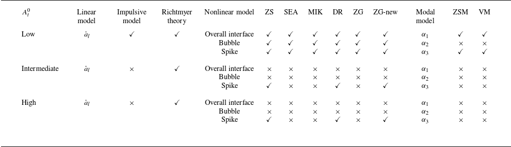
Summary of the predictive capabilities of considered linear, nonlinear and modal models for the interface evolution under different
 $A_t^0$
conditions. Here,
 $\checkmark$
indicates that the model is applicable, and
 $\times$
indicates that the model is inapplicable.

At low
 $A_t^0$
, the interface evolves slowly and overall resembles that observed under weak-shock conditions. In contrast, at moderate to high
 $A_t^0$
, compressibility effects markedly modify the interface morphology. Table 4 summarises the predictive capabilities of the considered linear, nonlinear and modal models for strong-shock RMI under diverse
 $A_t^0$
conditions. For the linear amplitude evolution, the Richtmyer theory exhibits robust predictive accuracy across a broad parameter range, but relies on numerical computations. In contrast, the impulsive model possesses a simple formulation, but its validity depends on shock intensity
 $A_t^0$
, and contrast in specific heat ratios across the interface, thereby constraining its general applicability. To address these limitations, we propose a modified impulsive model that maintains practical simplicity while achieving favourable predictive accuracy under varying compressibility conditions. For the nonlinear evolution, the influence of compressibility is limited at low
 $A_t^0$
, but it progressively suppresses bubble growth and enhances spike evolution at higher
 $A_t^0$
. Meanwhile, the spike-acceleration effect becomes prominent at high
 $A_t^0$
, further promoting spike growth. Regarding the spike, several existing models reasonably predict the growth across all cases, and this agreement is physically meaningful for low and high
 $A_t^0$
scenarios, but coincidental for the intermediate
 $A_t^0$
case. By contrast, all existing models fail to reproduce bubble evolution at moderate to high
 $A_t^0$
, as they neglect compressibility effects persisting into the nonlinear regime. Based on experimental evidence, we propose an empirical bubble model that explicitly incorporates compressibility, improving predictive capability under strong-shock, moderate to high
 $A_t^0$
conditions. Modal analysis further reveals that compressibility alters interface morphology even when amplitude growth remains largely unaffected at low
 $A_t^0$
. At higher
 $A_t^0$
, compressibility suppresses first-order mode growth while promoting higher-order harmonic generation through flattening bubbles and narrowing spikes, leading to the breakdown of incompressible modal models. Overall, the combined insights from experimental observations and theoretical analyses yield three practical guidelines. First, the Richtmyer theory and the newly proposed impulsive model can be reliably applied under varying compressibility conditions. Second, while current models can predict spike growth, whether physical or incidental, the compressibility-aware model is essential for accurately capturing bubble dynamics under strong shocks. Third, the present modal models are inapplicable under strong-shock conditions, and future developments should explicitly account for compressibility-induced harmonic generation.
For a typical inertial confinement fusion (ICF) capsule, the interfaces that separate the ablator from the deuterium–tritium (DT) ice, and the DT ice from the DT gas, are both heavy–light ones, and the penetration of the spike, composed of relatively cold ablative material or DT fuel, into the hot spot represents a critical factor limiting energy gain (Zhou et al. Reference Zhou, Sadler and Hurricane2025). If the interface is of a light–heavy configuration, then spikes penetrate outwards, rendering their impact on energy gain substantially weaker than in the heavy–light configuration, while bubbles tend to develop towards the hot-spot region. The present study indicates that bubble growth is markedly suppressed under strong-shock conditions. Therefore, wherever feasible, employing a lower-density ablator to establish a light–heavy interface between the shell and DT ice can effectively mitigate the detrimental effects of hydrodynamic instabilities on energy gain. On the other hand, based on our previous studies (Chen et al. Reference Chen, Xing, Wang, Zhai and Luo2023; Xing et al. Reference Xing, Chen, Li, Wang, Zhai and Luo2025) and present investigation across a wide range of
 $A_t^0$
values, spike acceleration exhibits a pronounced dependence on
 $A_t^0$
, which in turn governs the velocity of the spike and its penetration capability. Thus for heavy–light interfaces that are unavoidable, minimising the density contrast across the interface constitutes a practical strategy to mitigate the adverse effects of spike penetration on energy gain. To date, RMI on heavy–light interfaces spanning a broad range of
 $A_t^0$
values has been examined only under weak-shock conditions (Xing et al. Reference Xing, Chen, Li, Wang, Zhai and Luo2025), and a corresponding investigation under strong-shock conditions is currently underway. Unfortunately, due to the shock-proximity phenomenon, the gas-layer scheme is not applicable. Consequently, the upstream gas can only be air. Although low to moderate
 $A_t^0$
values can be achieved under this constraint, generating a heavy–light interface with high
 $A_t^0$
necessitates a novel approach, with ongoing efforts to address this challenge.
Supplementary movies
Supplementary movies are available at https://doi.org/10.1017/jfm.2025.10940.
Funding
This work is supported by the National Natural Science Foundation of China (nos 12388101, 12027801, U2430202 and 12472228), the Chinese Academy of Sciences Project for Young Scientists in Basic Research (YSBR-087), and Young Elite Scientists Sponsorship Programme by CAST (no. 2023QNRC001).
Declaration of interests
The authors report no conflict of interest.
Appendix A. Experimental evidence regarding completeness of polyester combustion
To further assess whether the polyester film is completely combusted in the current experiments, a comparative analysis is conducted with a previous experiment using the same shock tube and interface-formation technique, but employing a different gas combination at the interface (air–He). Figure 7 presents representative frames from the present experiment (case 0.35) and the reference experiment. The film fragments are clearly visible in the reference experiment, whereas they are absent in the present experiment. This difference is attributed to the substantially lower post-shock temperature in the reference experiment, with temperatures on the upstream and downstream sides of the shocked film of approximately 744 K and 740 K, respectively. Accordingly, the pyrolysis and combustion of the polyester film proceed much more slowly, leading to a considerable amount of residual film remaining. These observations provide indirect yet compelling evidence that the film undergoes near-complete combustion in the present experiments.
Representative images from experiments with interfaces of various gas combinations: (a) present experiment with an air–
 ${\textrm{SF}}_6$
interface; (b) reference experiment with an air–He interface. Numbers represent time in
 $\unicode{x03BC}$
s.

Appendix B. Experimental uncertainties
B.1. Shock and interface velocities
Take the determination of the experimental incident shock velocity (
 $v^e_{\textit{is}}$
) as an example:
 $v^e_{\textit{is}}$
is determined from the positions of the incident shock in two successive shadowgraphs before the shock interacts with the interface. The associated uncertainty stems from the finite thickness of the shock front in the shadowgraphs, which is approximately one pixel in width and corresponds to the spatial resolution
 $\Delta x$
. This results in an estimated uncertainty of less than 0.8 %. The experimental transmitted shock and shocked interface velocities (
 $v^e_{\textit{ts}}$
and
 $u^e_{\textit{si}}$
) are determined using a similar methodology, with their uncertainties both estimated to be less than 1.5 %.
B.2. Shadowgraph timing
The temporal origin (
 $t = 0$
 $\unicode{x03BC}$
s) is defined as the instant when the incident shock reaches the mean position of the initial interface (
 $x = x_i^0$
). The methodology to determine the timing of shadowgraphs is as follows. The position of the incident shock in the last shadowgraph before it reaches the mean position of the initial interface (
 $x_{\textit{is}}^0$
) is first extracted, with associated uncertainty
 $0.5\,\Delta x$
. Subsequently, the corresponding timing is calculated as
 $(x_{\textit{is}}^0 - x_i^0)/v^e_{\textit{is}}$
, with estimated uncertainty approximately 0.5
 $\unicode{x03BC}$
s. Since the time interval between shadowgraphs is identical, the timings of the remaining shadowgraphs can thus be determined, each with uncertainty 0.5
 $\unicode{x03BC}$
s.
B.3. Gas component
Due to the favourable sealing property of the polyester film, the upstream gas is considered as pure air, and the volume fraction of the downstream heavy gas (
 $\textit{VF}$
) is determined by solving the shock–interface interaction using one-dimensional gas dynamics theory. A MATLAB routine takes
 $v^e_{\textit{is}}$
as an input and determines
 $\textit{VF}$
by matching
 $v^e_{\textit{ts}}$
with the counterpart predicted by one-dimensional gas dynamics theory (
 $v^t_{\textit{ts}}$
). Therefore, the uncertainty of
 $\textit{VF}$
primarily arises from the uncertainties associated with
 $v^e_{\textit{is}}$
and
 $v^e_{\textit{ts}}$
. The uncertainties of
 $v^e_{\textit{is}}$
and
 $v^e_{\textit{ts}}$
, as discussed in § B.1, are estimated to be less than 0.8 % and 1.5 %, respectively. Based on these estimates, the overall uncertainty of
 $\textit{VF}$
is thereby calculated to be below 5 %.
B.4. Amplitude extraction
The interface amplitude is defined as half of the horizontal distance between the tips of the spike and bubble, with the corresponding uncertainty arising from the positional uncertainties of these tips.
For cases with low
 $A_t^0$
, the interface edge is well defined, and the upstream edge of the spike tip and the downstream edge of the bubble tip each span a single pixel, corresponding to the spatial resolution
 $\Delta x$
. Accordingly, the spike and bubble coordinates can be expressed as
 $x_s \pm 0.5\,\Delta x$
and
 $x_b \pm 0.5\,\Delta x$
, respectively, where
 $x_s$
(
 $x_b$
) denotes the coordinate of the spike (bubble) tip. The resulting interface mixing width is
 $x_b - x_s$
, with uncertainty
 $\pm \Delta x$
, and the interface amplitude is
 $(x_b - x_s)/2$
, with uncertainty
 $\pm 0.5\,\Delta x$
. Beyond the positional uncertainties of the spike and bubble tips, the uncertainties of the spike and bubble amplitudes also depend on the uncertainty in the mean position of the interface (
 $x_i$
). At early times,
 $x_i$
is given by
 $(x_b + x_s)/2 \pm 0.5\,\Delta x$
, from which the velocity of the mean position of the interface, i.e.
 $u^e_{\textit{si}}$
, can be obtained. Subsequently,
 $x_i$
at later times is determined by extrapolating the early-time
 $x_i$
using
 $u^e_{\textit{si}}$
. On this basis, the amplitudes of the spike and bubble are calculated as
 $x_i - x_s$
and
 $x_b - x_i$
, respectively, each with uncertainty
 $\pm \Delta x$
.
For cases with high
 $A_t^0$
, the interface edge is initially well defined but progressively blurs as the interface evolves, particularly the spike edge. Figure 8 shows the extracted positions of the spikes and bubbles at diverse temporal snapshots for case 0.71. The coordinate of the spike (bubble) tip is extracted from the intersection of regions with very low and relatively high grey values on the upstream (downstream) side of the interface. As this intersection becomes blurred, its positional uncertainty increases from one to two or three pixels, resulting in the uncertainties of
 $x_s$
and
 $x_b$
increasing from
 $\pm 0.5\,\Delta x$
to
 $\pm \Delta x$
or
 $\pm 1.5\,\Delta x$
. Consequently, the uncertainty of the interface amplitude becomes
 $\pm \Delta x$
or
 $\pm 1.5\,\Delta x$
, and the uncertainty of the bubble/spike amplitude becomes
 $\pm 2\,\Delta x$
or
 $\pm 3\,\Delta x$
.
Overall, the uncertainty of the overall interface, spike and bubble amplitudes is primarily determined by the sharpness of the interface edge: a well-defined edge corresponds to a small uncertainty, whereas a blurred edge results in a larger uncertainty.
Extracted positions of the spikes and bubbles at diverse temporal snapshots for case 0.71. Numbers represent time in
 $\unicode{x03BC}$
s.

Appendix C. Influence of shock intensity differences across experiments
The shock Mach numbers
 $M$
of the five experiments span from 3.16 to 3.41. This variation is chiefly due to two primary factors. First, variations arise from slight differences in the thickness of the aluminium diaphragm. Second, there are fluctuations in burst pressure owing to differences in the filling rate. Consequently, it is difficult to generate shocks of closely matched strength in separate experiments.
To evaluate the influence of differences in
 $M$
on the comparability of experiments with diverse
 $A_t^0$
, the linear growth rates predicted by Richtmyer theory using the actual
 $M$
and the average value of the lowest and highest
 $M$
(
 $3.29 = (3.16+3.41)/2$
), referred to as
 $\dot {a}_l^{r}$
and
 $\dot {a}_l^{ave}$
, respectively, are compared. Their deviation directly reflects the effect of fluctuations in
 $M$
on the overall interface evolution. As presented in table 5, the differences in the linear growth rates arising from fluctuations in
 $M$
are approximately 2.7 % on average. This finding suggests that slight variations in
 $M$
do not significantly affect the interface evolution, thereby justifying comparative analyses among different cases.
Comparison between linear growth rates predicted by the Richtmyer theory using the actual
 $M$
(
 $\dot {a}_l^{r}$
) and the average value of the lowest and highest
 $M$
(
 $\dot {a}_l^{ave}$
). Here,
 $E^{ave} = (\dot {a}_l^{ave}-\dot {a}_l^{r})/\dot {a}_l^{r}$
is the relative error between
 $\dot {a}_l^{ave}$
and
 $\dot {a}_l^{r}$
.

Appendix D. Influence of specific heat ratio variation
In the present experiments with
 $M$
exceeding 3.0, the elevated post-shock temperature is sufficient to induce molecular vibrational excitation in the experimental gases (e.g. air, CO
 $_2$
, SF
 $_6$
and C
 $_4$
F
 $_{10}$
), leading to variations in the specific heat ratio
 $\gamma$
. To evaluate the influence of variations in
 $\gamma$
on the interface evolution, the post-shock temperatures and pressures are first calculated, after which the effective post-shock
 $\gamma$
is determined. Subsequently, the Richtmyer theory predictions using the pre- and post-shock effective
 $\gamma$
(
 $\dot {a}_{l}^{r}$
and
 $\dot {a}_{l}^{\textit{post}}$
) are calculated, and the relevant parameters and detailed results are summarised in table 6. The results indicate that the alteration in the linear growth rate arising from the variation in effective
 $\gamma$
is less than 3.5 % on average, suggesting that this variation exerts a negligible influence on the interface evolution.
Comparison between linear growth rates predicted by the Richtmyer theory using pre- and post-shock effective
 $\gamma$
(
 $\dot {a}_l^{r}$
and
 $\dot {a}_l^{\textit{post}}$
). Here,
 $\gamma _{u/d}$
and
 $\gamma ^{\textit{post}}_{u/d}$
are pre- and post-shock effective
 $\gamma$
of the fluid upstream/downstream of the interface, respectively, and
 $E^{\textit{post}} = (\dot {a}_l^{\textit{post}}-\dot {a}_l^{r})/\dot {a}_l^{r}$
is the relative error between
 $\dot {a}_l^{\textit{post}}$
and
 $\dot {a}_l^{r}$
.

Variations of dimensionless linear amplitude growth rate
 $\alpha _l$
with shock intensity
 $\varepsilon$
: numerical results and corresponding Richtmyer theory predictions with
 $\gamma _d$
of (a) 1.29, (b) 1.15, and (c) 1.07.

Appendix E. Numerical simulations
The numerical solver referred to as HOWD (Ding et al. Reference Ding, Si, Chen, Zhai, Lu and Luo2017) is employed to simulate the interaction between a shock wave and a single-mode light–heavy interface. Its accuracy and reliability have been validated via various experiments (Ding et al. Reference Ding, Liang, Chen, Zhai, Si and Luo2018; Feng et al. Reference Feng, Xu, Zhai and Luo2021; Wang et al. Reference Wang, Wang, Zhai and Luo2023). The computational domain is a rectangle measuring 200 mm in length and 40 mm in height, consistent with that adopted in a previous study (Wang et al. Reference Wang, Wang, Zhai and Luo2023). The upper and lower boundaries are modelled as solid walls, whereas the others are treated as open. The grid resolution is determined based on grid convergence studies conducted in previous works (Ding et al. Reference Ding, Liang, Chen, Zhai, Si and Luo2018; Feng et al. Reference Feng, Xu, Zhai and Luo2021; Wang et al. Reference Wang, Wang, Zhai and Luo2023). To ensure numerical accuracy while minimising computational cost, an initial mesh size 0.1 mm is adopted.
Three sets of simulations are conducted, in which
 $\gamma _u$
is fixed at 1.40, while
 $\gamma _d$
is set to 1.29, 1.15 and 1.07, respectively. For each set of simulations, five values of
 $A_t^0$
(0.20, 0.35, 0.51, 0.67 and 0.71) and four shock intensities
 $\varepsilon$
(defined as
 $1 - p_0/p_1$
, where
 $p_0$
and
 $p_1$
represent the pressures of gases in front of and behind the incident shock, respectively), 0.2, 0.5, 0.8 and 0.95, are considered. To facilitate comparison, we adopt the approach of Mikaelian (Reference Mikaelian1994) to normalise
 $\alpha_l = \dot {a}_l/ka_0u_{si}$
, and the results obtained from simulations and predicted by the Richtmyer theory are plotted in figure 9 as functions of
 $\varepsilon$
. The numerical results are in favourable agreement with the predictions of the Richtmyer theory across all cases. This indicates that the Richtmyer theory remains consistently valid over a wide range of conditions, and therefore can serve as a reliable benchmark for assessing the predictive capability of the impulsive model.