1 Introduction
Understanding, predicting and eventually delaying the laminar–turbulent transition in boundary-layer flows has long been a challenge for researchers. For small-amplitude disturbances and supercritical Reynolds numbers, the linear stability theory predicts a slow transition process due to the generation, amplification and secondary instability of Tollmien–Schlichting (TS) waves. It is however known that this transition process can be greatly modified by environmental noise or by the presence of localized or distributed surface roughness. Depending on the flow’s characteristics and the nature of the surface roughness, the transition process can either be promoted or delayed.
Klebanoff & Tidstrom (Reference Klebanoff and Tidstrom1972) have shown experimentally that this natural transition could be promoted using spanwise invariant roughness elements. This transition is related to the modified stability properties of the boundary-layer flow developing downstream of the roughness element, enhancing the unstable TS waves. More recently, Perraud et al. (Reference Perraud, Arnal, Séraudie and Tran2004) have shown that the higher the two-dimensional roughness element, the closer to it does transition to turbulence take place. The influence of fully three-dimensional roughness elements on the transition to turbulence differs quite significantly. While fully three-dimensional roughness elements hardly promote flow separation, they induce streamwise high-speed and low-speed streaks. In their seminal paper, Cossu & Brandt (Reference Cossu and Brandt2004) have shown that these streaks may stabilize the TS waves and thus delay the natural transition process. Experimental confirmation of the stabilization capabilities of such roughness elements have been provided by Fransson et al. (Reference Fransson, Brandt, Talamelli and Cossu2004) and Shahinfar, Fransson & Talamelli (Reference Shahinfar, Fransson and Talamelli2012), making these an interesting device for passive flow control. Despite their stabilizing effect on TS waves, in certain flow conditions (Reynolds number, height, shape and aspect ratio of the protuberance) transition to turbulence can occur right downstream of the roughness elements, a detrimental effect for control purposes.
The flow pattern induced by an isolated three-dimensional roughness element has been known for almost 60 years (Gregory & Walker Reference Gregory and Walker1955). When impinging the three-dimensional roughness element, the spanwise vorticity of the incoming boundary layer wraps around it, thus creating horseshoe vortices. As shown by Baker (Reference Baker1978), their characteristics and number are essentially dependent on the aspect ratio of the roughness element considered. Nonetheless, they all give birth further downstream to quasi-aligned streamwise vortices. Due to the lift-up effect (Landahl Reference Landahl1975), these streamwise aligned vortices can trigger strong transient growth of the boundary-layer streaks (Joslin & Grosch Reference Joslin and Grosch1995), strong enough to yield their breakdown and subsequent transition to turbulence. The receptivity of the boundary-layer flow to three-dimensional roughness elements and the associated transient growth of the velocity streaks have been thoroughly investigated by various authors such as Fischer & Choudhari (Reference Fischer and Choudhari2004), Tumin & Reshotko (Reference Tumin and Reshotko2005), Ergin & White (Reference Ergin and White2006) as well as Denissen & White (Reference Denissen and White2008, Reference Denissen and White2009). Their major finding is that the streamwise transient growth of the induced streaks roughly scales with the square of the roughness Reynolds number,
 $Re_{h}^{2}$
(where
 $Re_{h}=U_{Bl}(h)h/\unicode[STIX]{x1D708}$
,
 $U_{Bl}(h)$
being the value of the Blasius velocity profile evaluated at the roughness element’s position and height
 $h$
, and
 $\unicode[STIX]{x1D708}$
is the kinematic viscosity). The crucial importance of the roughness Reynolds number in the roughness-induced transition to turbulence had already been outlined many years earlier.
In an effort to provide thresholds for transition, von Doenhoff & Baslow (Reference von Doenhoff and Baslow1961) compiled a transition diagram correlating the roughness element’s aspect ratio to the roughness Reynolds number,
 $Re_{h}$
, beyond which the induced flow would transition to turbulence. However, such a transition diagram shows a rather wide transition region within which some experiments have reported transitioning flows (Tani, Komoda & Komatsu Reference Tani, Komoda and Komatsu1962) whereas others have observed laminar flows (Klebanoff, Cleveland & Tidstrom Reference Klebanoff, Cleveland and Tidstrom1992).
Vermeersch (Reference Vermeersch2009) and Arnal et al. (Reference Arnal, Houdeville, Séraudie and Vermeersch2011) have shown that the onset of transition may be explained by the optimal perturbation theory. Although promising, their approach relies on the strong assumption of quasi-parallelism of the flow induced by the three-dimensional roughness element and on the empirical
 $N$
-factor (van Ingen Reference van Ingen1956; Smith & Gamberoni Reference Smith and Gamberoni1956). Cherubini et al. (Reference Cherubini, De Tullio, De Palma and Pascazio2013) have used the optimal perturbation theory as well but applied it to the fully three-dimensional flow field surrounding a relatively large smooth-edged roughness element. In this three-dimensional framework, the optimal perturbation takes the form of a wavepacket-like structure initially localized in the vicinity of the separation line on the top of the roughness element. As it travels downstream, this perturbation can trigger localized transition and induce hairpin vortices once nonlinearities are taken into account. However, due to the linearly stable nature of the flow considered, the unsteadiness observed is not self-sustaining once these linear transients have been washed out from the computational domain. In the meantime, de Tullio et al. (Reference de Tullio, Paredes, Sandham and Theofilis2013) have investigated the roughness-induced transition in the case of a compressible boundary-layer flow using the joint application of local stability analysis, parabolized stability equations and direct numerical simulations. These authors have shown that the flows they have investigated are much more convectively unstable, be it to varicose or sinuous perturbations, than the classic boundary-layer flow. Such analyses however still do not provide a transition threshold.
With the aim of providing a more accurate estimate of the critical Reynolds number for transition, global stability analyses have been recently performed in the case of cylindrical (Loiseau et al. Reference Loiseau, Robinet, Cherubini and Leriche2014) and hemispherical (Citro et al. Reference Citro, Giannetti, Luchini and Auteri2015) roughness elements. As discussed in Loiseau et al. (Reference Loiseau, Robinet, Cherubini and Leriche2014), the critical Reynolds numbers computed by stability analysis lie close to the upper limit of the transition band of the diagram, suggesting that a fully three-dimensional global instability analysis might be able to provide an estimate for the upper threshold. However, despite the many numerical (de Tullio et al. Reference de Tullio, Paredes, Sandham and Theofilis2013), experimental (Ye, Schrijer & Scarano Reference Ye, Schrijer and Scarano2016) and instability (Cherubini et al. Reference Cherubini, De Tullio, De Palma and Pascazio2013) studies on this subject, how and why transition is triggered close to the lower limit of the stability diagram remains to be understood. Note finally that similar analyses have been conducted for roughness-induced compressible boundary-layer flows. One can cite for instance the works of Bernardini, Pirozzoli & Orlandi (Reference Bernardini, Pirozzoli and Orlandi2012), Subbareddy, Bartkowicz & Candler (Reference Subbareddy, Bartkowicz and Candler2014), Kurz & Kloker (Reference Kurz and Kloker2016) and references therein for more details.
In this paper, we aim at giving an explanation for the onset of unsteadiness and subsequent transition to turbulence at subcritical values of the Reynolds number, where the critical value is that provided by a global stability analysis. In order to validate the predictions of the stability analysis, the flow behind a roughness element has also been investigated experimentally in a water channel and numerically by means of direct numerical simulation (DNS). As to reduce the parameter space of this study and referring to results in the literature (Tani et al. Reference Tani, Komoda and Komatsu1962; Loiseau et al. Reference Loiseau, Robinet, Cherubini and Leriche2014), our attention has been focused on cylindrical roughness elements of aspect ratio 1 and 3. These configurations are particularly interesting since the global stability analysis performed by Loiseau et al. (Reference Loiseau, Robinet, Cherubini and Leriche2014) has shown the existence of global eigenmodes with different symmetries, a varicose and a sinuous one. The paper is structured as follows: in § 2, the experimental set-up and numerical methods are presented; global stability and optimal forcing analysis are discussed in § 3.1; whereas, in § 3.2 direct numerical simulations provide insights into the nonlinear evolution of the flow. Finally, concluding remarks and perspectives are given in § 4.
2 Experimental set-up and observations
This section introduces the experimental facility, set-up and experimental observations. Three subcritical roughness configurations have been analysed and respective parameters are given in this section.
2.1 Facility and flow configuration
The laminar water channel (Laminarwasserkanal) is a closed circuit water channel at the Institute of Aerodynamics and Gas Dynamics (IAG) at the University of Stuttgart. The turbulence intensity is 0.089 % of the free-stream velocity in the frequency range 0.1–10 Hz at
 $0.0745~\text{m}~\text{s}^{-1}$
and the test section is
 $8\times 1.2\times 0.2$
m. To maintain the turbulence intensity even at very low free-stream velocities, an additional screen is installed if the free-stream velocity is below
 $0.06~\text{m}~\text{s}^{-1}$
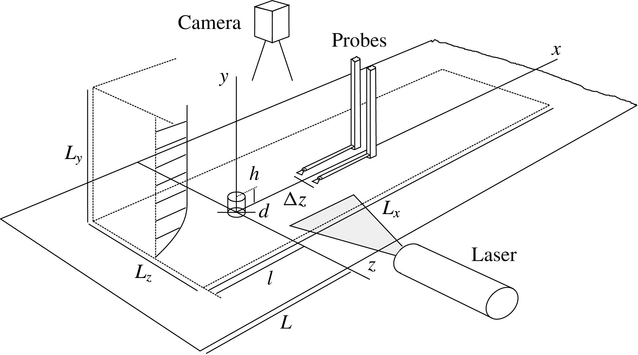
as described in Puckert, Dieterle & Rist (Reference Puckert, Dieterle and Rist2017). A steady two-dimensional laminar boundary layer of Blasius type is created by a flat plate with an elliptical leading edge. The experimental set-up and the corresponding computational domain are sketched in figure 1. All length scales are non-dimensionalized by the constant roughness height
 $h$
, which equals 10 mm in the physical experiment and 1 in the numerical simulation. The roughness position is constant at
 $L=57.1h$
from the leading edge. Three different configurations are investigated with parameters reported in table 1. The aspect ratio
 $\unicode[STIX]{x1D702}=d/h$
is given by the roughness diameter
 $d$
and the Reynolds number
 $Re=hU_{e}/\unicode[STIX]{x1D708}$
is determined by the (variable) free-stream velocity
 $U_{e}$
and the dynamic viscosity
 $\unicode[STIX]{x1D708}$
of water. Due to the temperature dependency of the dynamic viscosity, its value is determined prior to each individual experiment. The coordinate system originates from the bottom centre of the roughness with non-dimensional
 $x$
-,
 $y$
- and
 $z$
-coordinates extending in streamwise, wall-normal and spanwise direction, respectively.
Hot-film measurements have been performed with a Dantec Streamline 90N10 system and two single-wire probes 55R15 which were calibrated with a traverse system in resting water as described in Subasi et al. (Reference Subasi, Puckert, Gunes and Rist2015). The voltage signals are recorded by a 16-bit A/D-converter at 100 Hz and digitally filtered between 0.1 and 10 Hz. The voltage signal is converted into a streamwise velocity by applying King’s law and decomposed into mean velocity
 $\overline{u}$
and disturbance signal
 $u^{\prime }$
. Particle image velocimetry (PIV) has been performed with dual-pulse Nd:YAG Quantel Twin lasers (532 nm), a PCO Sensicam system for image acquisition and the flow has been seeded with
 $4.2~\unicode[STIX]{x03BC}\text{m}$
nylon particles.
Sketch of experimental set-up and computational domain. Domain size:
 $L_{x}=115$
,
 $L_{y}=40$
,
 $L_{z}=10$
,
 $l=-25$
,
 $L=-57.1$
.
 $\unicode[STIX]{x0394}z$
is varied during experiments.

2.2 Experimental observations
The effect of the cylinder on the laminar boundary layer for the configuration
 $(\unicode[STIX]{x1D702},Re)=(1,700)$
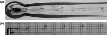
is visualized with potassium permanganate crystals on top of and around the roughness, which dissolve in water and draw dye streaklines into the flow field. In figure 2(a), crystals upstream of the roughness visualize the contour around a steady horseshoe vortex wrapping around the roughness with nearly straight trailing legs. Similarly, the recirculation zone can be seen as a dark region downstream of the roughness followed by regular ejection of hairpin vortices. These unsteady vortices consist of an omega-shaped head in the upper region of the boundary layer and legs in the lower region and have been analysed in detail by Acarlar & Smith (Reference Acarlar and Smith1987) for instance. Figure 2(b) shows the shedding of hairpin vortices from a side view. From this picture, the vortex wavelength can be estimated by the spacing of the heads, which is approximately
 $\unicode[STIX]{x1D706}_{x}\simeq 4.8$
. In both figures 2(a) and 2(b), the shape of the hairpin vortices becomes less pronounced as they travel downstream, which is a manifestation of transition to turbulence. As proposed by Klebanoff et al. (Reference Klebanoff, Cleveland and Tidstrom1992), the lower part is more affected by turbulent mixing than the upper part, therefore the hairpin heads preserve their shape for a longer distance than the legs. The same visualizations have been repeated for the other configurations and visual estimates of the wavelength are provided in table 1. The spanwise symmetry property of the unsteady disturbances has been measured for the same configuration
 $(\unicode[STIX]{x1D702},Re)=(1,700)$
by two single-wire hot-film probes located symmetrically with respect to the
 $z=0$
plane in the wake of the roughness element. Their separation
 $\unicode[STIX]{x0394}z$
was increased from 0.5 to 6.5 in steps of
 $\unicode[STIX]{x0394}(\unicode[STIX]{x0394}z)=0.5$
and traversed vertically in increments of
 $\unicode[STIX]{x0394}y=0.2$
at three downstream positions
 $x=10$
,
 $x=20$
and
 $x=30$
. At each position, the two disturbance signals
 $u_{1}^{\prime }$
and
 $u_{2}^{\prime }$
of the probes have been acquired for 30 s and separated into a symmetric (varicose,
 $u_{v}$
) and antisymmetric (sinuous,
 $u_{s}$
) component according to the following approach (Shin, Rist & Krämer Reference Shin, Rist and Krämer2015):
 $$\begin{eqnarray}\displaystyle u_{v}=\left(\frac{u_{1}^{\prime }+u_{2}^{\prime }}{2}\right)_{rms},\quad u_{s}=\left(\frac{u_{1}^{\prime }-u_{2}^{\prime }}{2}\right)_{rms}, & & \displaystyle\end{eqnarray}$$
where rms refers to the root mean square value.
Flow visualization for the case
 $(\unicode[STIX]{x1D702},Re)=(1,1700)$
with potassium permanganate crystals placed upstream of roughness and in recirculation zone. (a) Top view and (b) side view with 5 mm grid background.

Summary of the flow parameters, circular frequencies and wavelengths.

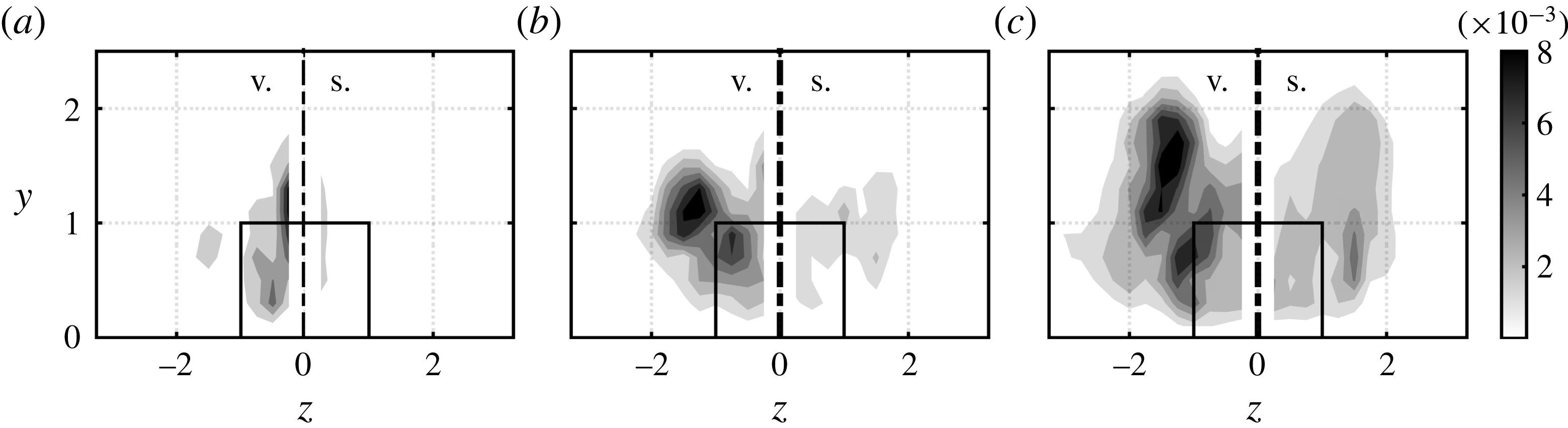
The result of this decomposition is shown in figure 3. Here, the varicose (sinuous) component is plotted on the left (right) of the spanwise symmetry plane for
 $x=10$
, 20 and 30. Note that both components actually exist on both sides and that the probe spacing leads to an inevitable gap around the spanwise centre. For all three downstream positions, the varicose disturbance dominates over the sinuous one. The position of maximum varicose disturbance is in agreement with the position of the heads and legs of the hairpin vortices in figure 2 and its amplitude grows in the downstream direction. The leading unsteadiness of the flow is therefore of varicose nature, as also found in the other configurations considered here. The increasing amplitude of the sinuous component with increasing
 $x$
is likely due to nonlinear interaction of unsteady disturbances, typical for laminar–turbulent breakdown. In the limit of fully developed turbulence, the quantities in (2.1) should become identical.
Grey scales for the case
 $(\unicode[STIX]{x1D702},Re)=(1,1700)$
showing varicose (v.) and sinuous (s.) disturbance components according to (2.1) on left and right side of the spanwise symmetry plane (dash-dotted line), respectively, at three downstream positions: (a)
 $x=10$
, (b)
 $x=20$
and (c)
 $x=30$
.

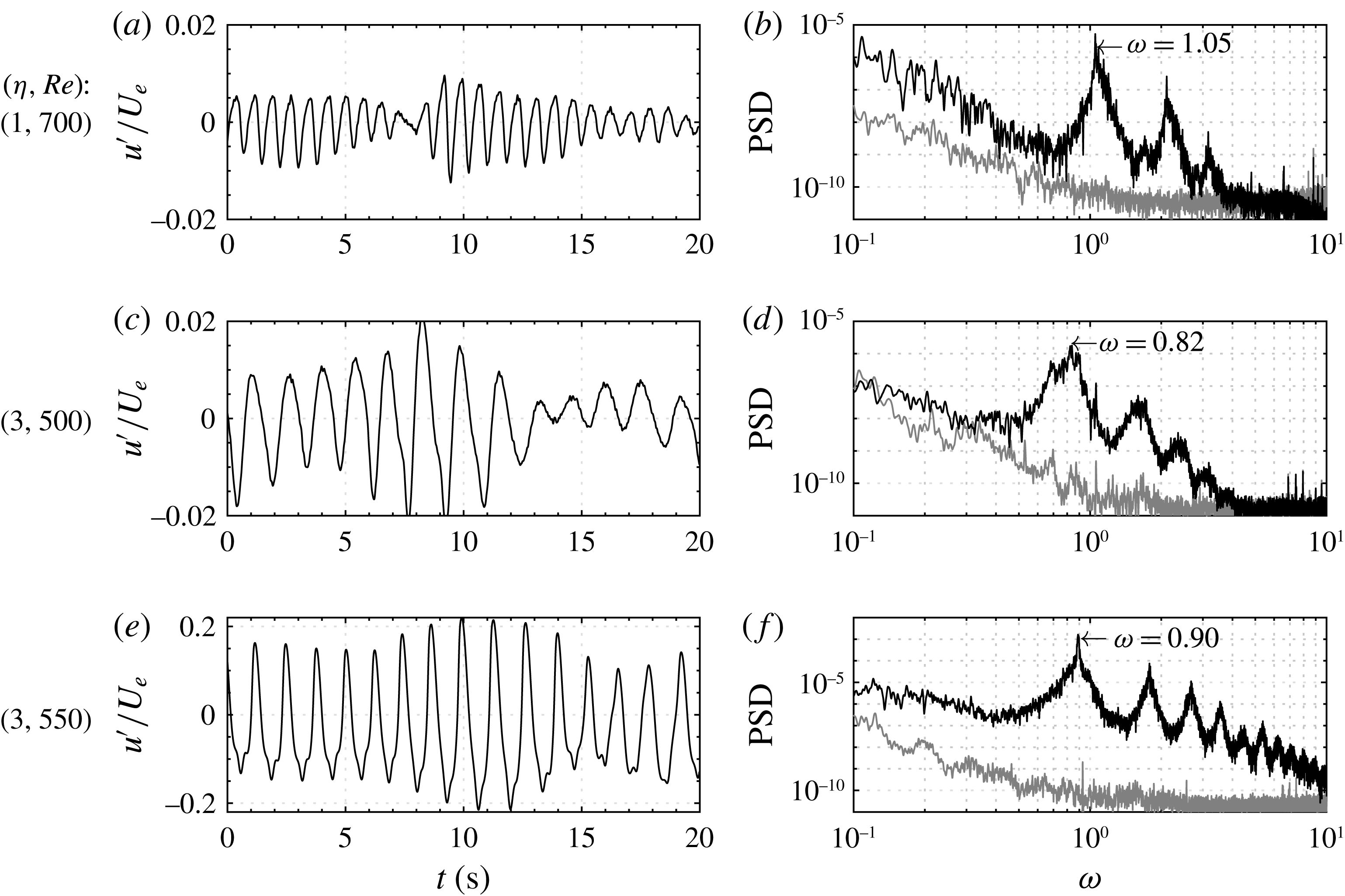
Figure 4(a,c,e) shows time traces of the streamwise velocity fluctuations for each configuration measured downstream of the respective roughness element. Only the first 20 out of 1200 s are shown, but the signals look similar in the remaining parts. In all cases, the time traces show fluctuations at a distinct frequency with temporally varying amplitudes. The amplitude fluctuations are typical for experiments where the background noise is inevitably uncontrolled and thus different from typical numerical time traces. The sensitivity to background noise is an important feature with major implications on the roughness-induced transition. This will be discussed from a theoretical perspective in the following sections. Note that the ordinate of the configuration
 $(\unicode[STIX]{x1D702},Re)=(3,550)$
is not identical to the other two configurations. This case is close to the critical Reynolds number
 $Re_{c}=564$
determined by Loiseau et al. (Reference Loiseau, Robinet, Cherubini and Leriche2014) and therefore fluctuates stronger and with more constant amplitude. On the contrary, for
 $(\unicode[STIX]{x1D702},Re)=(3,500)$
, the oscillations have a significantly smaller amplitude. They moreover sustain themselves only transiently, rapidly fading away before being regenerated again. Figure 4(b,d,f) shows Fourier spectra of the respective signals with non-dimensional abscissas
 $\unicode[STIX]{x1D714}=2\unicode[STIX]{x03C0}f\,hU_{e}^{-1}$
, where
 $f$
is the physical frequency in Hertz. Spectral peaks can clearly be distinguished from background noise and in all configurations also higher harmonics of the fundamental fluctuation can be observed. The fundamental frequencies are summarized in table 1.
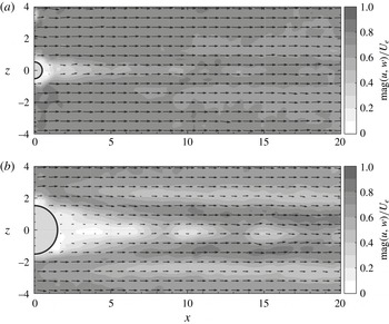
The unsteadiness is further illustrated by PIV snapshots in wall-normal planes at
 $y=1$
in figure 5. Grey scales indicate the in-plane velocity magnitude and black vectors indicate the vector sum of streamwise and spanwise velocities. In both snapshots one can see the streaky wake of the roughness elements with quasi-symmetrical oscillations around the spanwise centreline. Again, this unsteadiness belongs to the observation of hairpin vortices for both configurations. The question to be answered by theory is how this unsteadiness can be triggered and self-sustained despite the globally stable nature of the flow for the range of parameters considered herein (Loiseau et al.
Reference Loiseau, Robinet, Cherubini and Leriche2014).
(a,c,e) Time signals and (b,d,f) power spectral densities (PSD) of streamwise velocity fluctuations
 $u^{\prime }/U_{e}$
. Probe located at
 $(x,y,z)=(5,1.5,0)$
for case
 $(\unicode[STIX]{x1D702},Re)=(1,1700)$
and
 $(x,y,z)=(10,1.5,0)$
for the remaining cases. Grey lines in the spectra represent free-stream turbulence spectrum at
 $(x,y,z)=(0,6,0)$
.

PIV snapshots at
 $y=1$
for (a)
 $(\unicode[STIX]{x1D702},Re)=(1,700)$
, (b)
 $(\unicode[STIX]{x1D702},Re)=(3,500)$
.

3 Numerical investigation
The three experimental cases listed in table 1 are investigated by the joint use of direct numerical simulations, linear stability analysis and optimal forcing analysis with the aim of shedding some light on the onset of unsteadiness downstream of the roughness element. As sketched on figure 1, the computational domain considered is given by
 $L_{x}=[-25,~90]$
(
 $x=0$
being the cylinder position),
 $L_{y}=[0,~40]$
and
 $L_{z}=[-5,~5]$
,
 $x$
,
 $y$
and
 $z$
being the streamwise, wall-normal and spanwise directions, respectively. The dynamics of the incompressible flow is assumed to be governed by the Navier–Stokes equations
 $$\begin{eqnarray}\displaystyle \left.\begin{array}{@{}c@{}}\displaystyle \frac{\unicode[STIX]{x2202}\boldsymbol{U}}{\unicode[STIX]{x2202}t}+(\boldsymbol{U}\boldsymbol{\cdot }\unicode[STIX]{x1D735})\boldsymbol{U}=\unicode[STIX]{x1D735}P+\frac{1}{Re}\unicode[STIX]{x1D6FB}^{2}\boldsymbol{U},\\ \displaystyle \unicode[STIX]{x1D735}\boldsymbol{\cdot }\boldsymbol{U}=0,\end{array}\right\} & & \displaystyle\end{eqnarray}$$
where
 $\boldsymbol{U}(\boldsymbol{x},t)=(U,V,W)^{\text{T}}$
is the three-dimensional velocity field and
 $P(\boldsymbol{x},t)$
the pressure field. A Neumann boundary condition is used at the upper boundary of the computational domain while a no-slip condition is prescribed at the wall. In the spanwise direction, periodicity is imposed. Despite these periodic conditions, the spanwise extent of the domain is sufficiently large so that the roughness element almost behaves as though it is isolated (Braslow Reference Braslow1960). Finally, the conditions prescribed at the inflow and outflow boundaries of the computational domain depend on the analysis considered and will be stated whenever needed in the next sections. The Navier–Stokes equations are solved using the incompressible flow solver Nek5000 (Fischer et al.
Reference Fischer, Kruse, Mullen, Tufo, Lottes and Kerkemeier2008) which is based on the spectral element method (Patera Reference Patera1984; Deville, Fischer & Mund Reference Deville, Fischer and Mund2002). A
 $\mathbb{P}_{N}-\mathbb{P}_{N-2}$
formulation has been used: the velocity field is discretized using
 $N$
th degree Lagrange interpolants, defined on the Gauss–Legendre–Lobatto quadrature points, as basis and trial functions, while the pressure field is discretized using Lagrange interpolants of degree
 $N-2$
defined on the Gauss–Legendre quadrature points. All results presented hereafter are based on the polynomial degree
 $N=8$
, see appendix A for details about the grid convergence study. Finally, time integration is performed using the BDF3/EXT3 scheme: integration of the viscous terms relies on backward differentiation (BDF3), while the convective terms are integrated explicitly using a third-order accurate extrapolation (EXT3).
Owing to their linearly stable nature, see § 3.1, no selective frequency damping (Åkervik et al.
Reference Åkervik, Brandt, Henningson, Hoepffner, Marxen and Schlatter2006) or Newton method were required to compute most of the base flows
 $\boldsymbol{U}_{b}(\boldsymbol{x})$
considered in the rest of this work. These have simply been computed by time marching the Navier–Stokes equations until the norm of the residual drops below a given tolerance, in the present case
 $\Vert \unicode[STIX]{x2202}\boldsymbol{U}/\unicode[STIX]{x2202}t\Vert \leqslant 10^{-9}$
. This linearly stable nature of the flow is in apparent contradiction with the experimental observations reported in § 2.2. The following sections are devoted to the explanation of these differences.
3.1 Linear dynamics
The dynamics of infinitesimal perturbations evolving in the vicinity of a given base flow
 $\boldsymbol{U}_{b}$
is governed by the linearized Navier–Stokes equations
 $$\begin{eqnarray}\displaystyle \left.\begin{array}{@{}c@{}}\displaystyle \frac{\unicode[STIX]{x2202}\boldsymbol{u}}{\unicode[STIX]{x2202}t}+(\boldsymbol{u}\boldsymbol{\cdot }\unicode[STIX]{x1D735})\boldsymbol{U}_{b}+(\boldsymbol{U}_{b}\boldsymbol{\cdot }\unicode[STIX]{x1D735})\boldsymbol{u}=-\unicode[STIX]{x1D735}p+\frac{1}{Re}\unicode[STIX]{x1D6FB}^{2}\boldsymbol{u},\\ \unicode[STIX]{x1D735}\boldsymbol{\cdot }\boldsymbol{u}=0,\end{array}\right\} & & \displaystyle\end{eqnarray}$$
while their adjoint counterparts are given by
 $$\begin{eqnarray}\displaystyle \left.\begin{array}{@{}c@{}}\displaystyle \frac{\unicode[STIX]{x2202}\boldsymbol{u}^{\dagger }}{\unicode[STIX]{x2202}t}+(\unicode[STIX]{x1D735}\boldsymbol{U}_{b})^{\text{T}}\boldsymbol{u}^{\dagger }+(\boldsymbol{U}_{b}\boldsymbol{\cdot }\unicode[STIX]{x1D735})\boldsymbol{u}^{\dagger }=-\unicode[STIX]{x1D735}p^{\dagger }+\frac{1}{Re}\unicode[STIX]{x1D6FB}^{2}\boldsymbol{u}^{\dagger },\\ \unicode[STIX]{x1D735}\boldsymbol{\cdot }\boldsymbol{u}^{\dagger }=0,\end{array}\right\} & & \displaystyle\end{eqnarray}$$
where
 $\boldsymbol{U}_{b}$
is the base flow velocity field, while
 $(\boldsymbol{u},p)$
and
 $(\boldsymbol{u}^{\dagger },p^{\dagger })$
are the direct and adjoint velocity and pressure perturbations, respectively. Although one should traditionally use a Neumann condition at the outflow (inflow) for the direct (adjoint) equations, a zero velocity condition has been prescribed at both the inflow and outflow in all cases for the sake of computational simplicity during the optimal forcing analysis. Additionally, fringe regions have been used as to kill the (adjoint) perturbation once it reaches the outflow (inflow). Note that the streamwise extent of the domain and the characteristics of the fringe regions have been chosen so that our results are hardly influenced by the inflow–outflow boundary conditions, see appendix B for more details.
3.1.1 Eigenspectrum and eigenmodes
The linear stability of a base flow
 $\boldsymbol{U}_{b}$
is dictated by the fate of an infinitesimal perturbation
 $\boldsymbol{u}$
evolving in its vicinity. Once projected onto a divergence-free vector space, the linearized Navier–Stokes equations can be compactly written as
 $$\begin{eqnarray}\displaystyle \frac{\unicode[STIX]{x2202}\boldsymbol{u}}{\unicode[STIX]{x2202}t}=\unicode[STIX]{x1D63C}\boldsymbol{u}, & & \displaystyle\end{eqnarray}$$
with
 $\unicode[STIX]{x1D63C}$
being the projection of the linearized Navier–Stokes operator onto the divergence-free vector space. The asymptotic time evolution of an infinitesimal perturbation
 $\boldsymbol{u}$
is then governed by the eigenspectrum of
 $\unicode[STIX]{x1D63C}$
. Due to the very large dimensions of
 $\unicode[STIX]{x1D63C}$
once the linearized Navier–Stokes equations are discretized in space, its leading eigenpairs cannot be readily obtained using direct eigenvalue solvers. In order to circumvent this problem, a time stepper approach, popularized by Edwards et al. (Reference Edwards, Tuckerman, Friesner and Sorensen1994) and Bagheri et al. (Reference Bagheri, Schlatter, Schmid and Henningson2009), is used. This method aims at computing approximations of the leading eigenpairs of the exponential propagator
 $\boldsymbol{M}=\text{e}^{\unicode[STIX]{x1D63C}\unicode[STIX]{x0394}t}$
, whose action onto an initial vector is easily computed by time marching the linearized Navier–Stokes equations from
 $t=0$
to
 $t=\unicode[STIX]{x0394}t$
. Iterative eigenvalue solvers, such as the implicitly restarted Arnoldi method (Sorensen Reference Sorensen1992; Lechoucq & Sorensen Reference Lechoucq and Sorensen1996) or the Krylov–Schur decomposition (Stewart Reference Stewart2001), can then be used to project the propagator
 $\boldsymbol{M}$
onto an orthonormal set of vectors spanning a Krylov subspace of dimension
 $k$
, hence resulting in a low-dimensional
 $k\times k$
Hessenberg matrix
 $\unicode[STIX]{x1D643}$
. The eigenvalues
 $\unicode[STIX]{x1D706}=\unicode[STIX]{x1D70E}+\text{i}\unicode[STIX]{x1D714}$
of
 $\unicode[STIX]{x1D643}$
provide a good approximation to those of
 $\boldsymbol{M}$
. In this work, an in-house Krylov–Schur algorithm with a Krylov subspace dimension
 $k=400$
and a sampling period
 $\unicode[STIX]{x0394}t=0.748$
has been used.
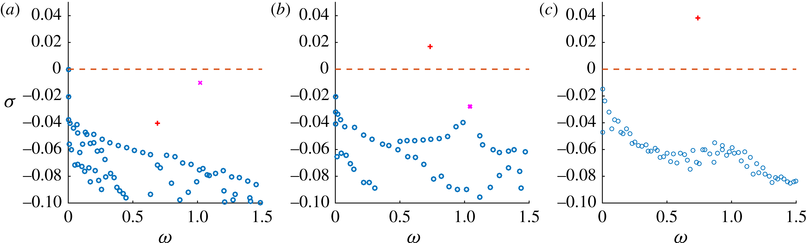
Figure 6(a) provides the eigenspectrum for case
 $(\unicode[STIX]{x1D702},Re)=(1,700)$
which does not present any unstable mode. At the bottom of the spectrum, one can observe a branch of modes characterized by a varicose symmetry (circles). On top of them, two isolated modes, characterized by different symmetries, can be seen: a varicose mode with
 $\unicode[STIX]{x1D714}=1.02$
lying close to the instability threshold (magenta cross), along with a more stable sinuous one (red plus) with
 $\unicode[STIX]{x1D714}=0.68$
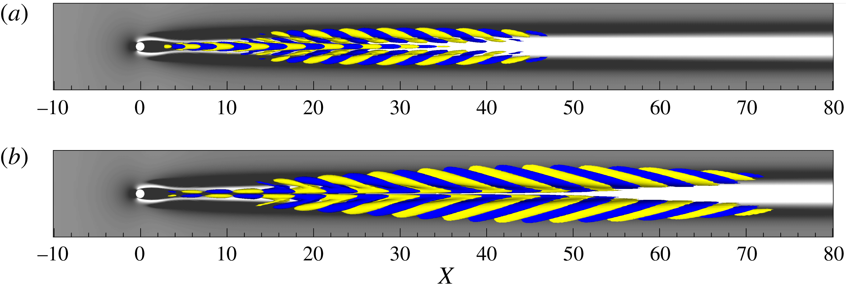
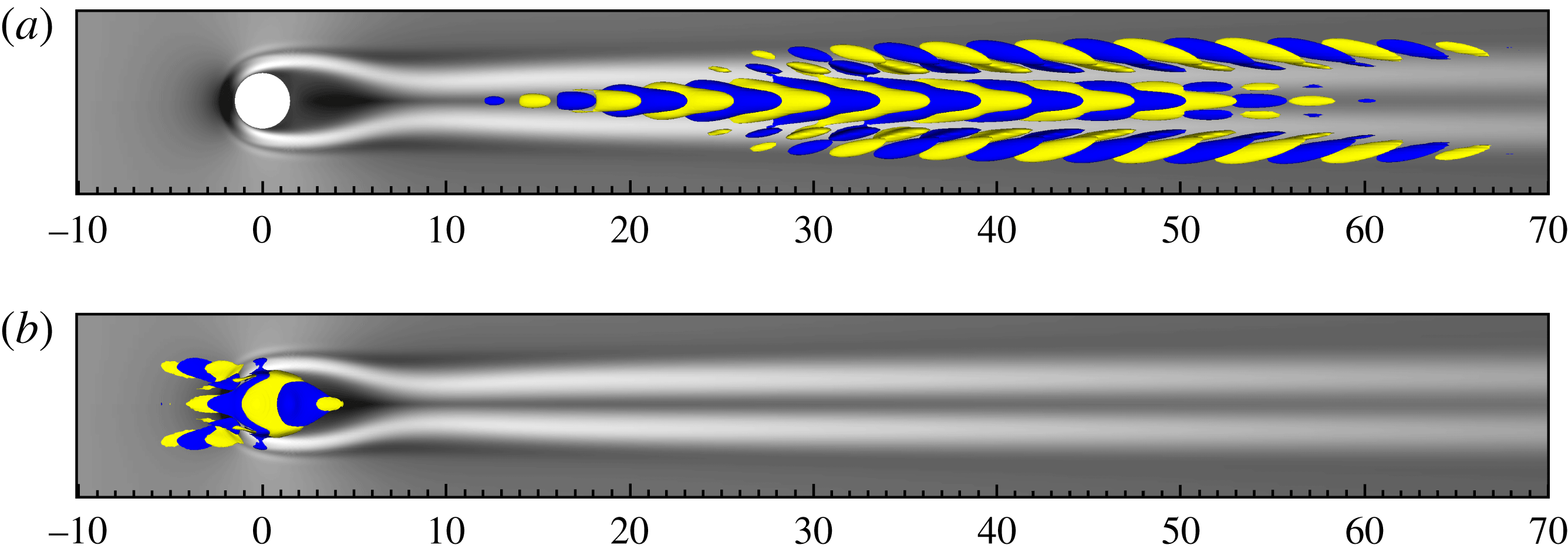
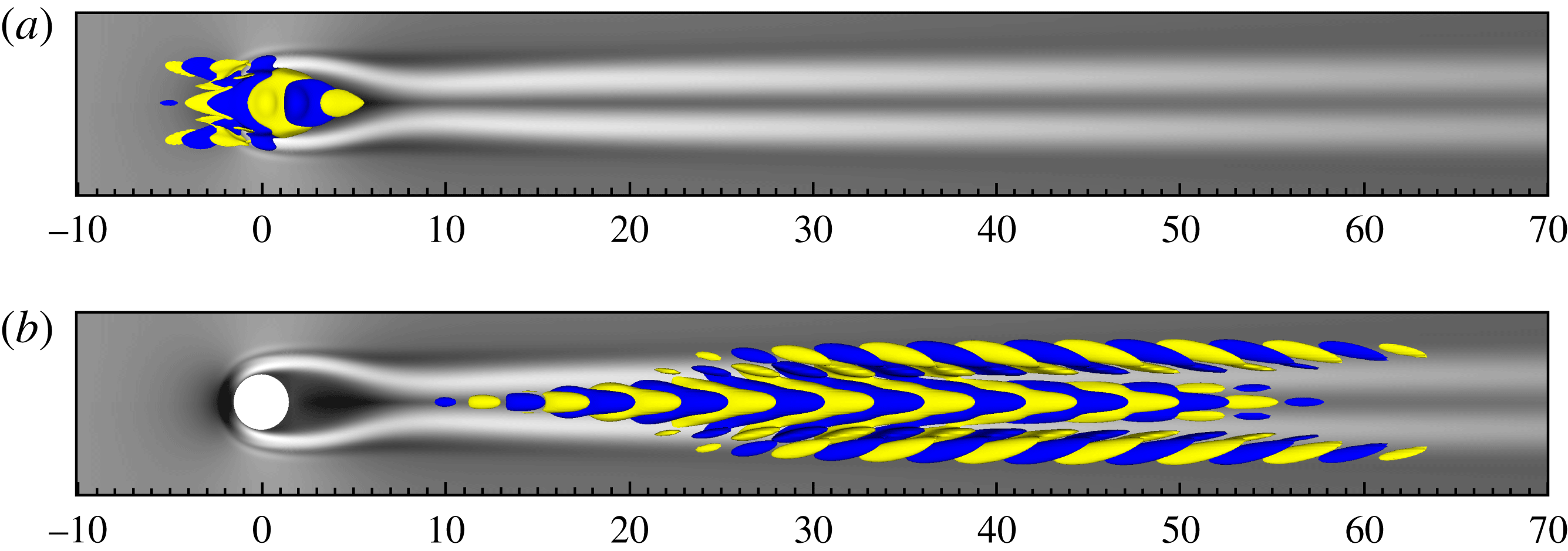
. The varicose leading eigenvector, depicted in figure 7(a), shows patches of spanwise-symmetric streamwise velocity perturbations, which are alternated in the streamwise direction. They are placed on top of the near-wake central low-speed streak of the base flow, as well as on the low-speed streaks placed at the sides of the central one further downstream (black isocontours). The sinuous one, shown in figure 7(b) exhibits a very similar shape, except for its opposite symmetry and its longer streamwise extent. The fact that the varicose mode lays much closer to the stability threshold than the sinuous one might suggest that, increasing the Reynolds number, the former will become unstable before the latter, driving the destabilization of the flow. However, a surprising behaviour can be inferred by inspecting figure 6, showing the spectra obtained for
 $Re=700$
,
 $900$
and
 $1200$
(from left to right). When increasing the Reynolds number, the sinuous mode quickly rises in the
 $\unicode[STIX]{x1D714}{-}\unicode[STIX]{x1D70E}$
plane, becoming unstable for
 $700<Re_{c}<900$
, whereas the isolated varicose mode moves down, joining the convective varicose branch at
 $900<Re<1200$
. This suggests that the varicose unsteadiness observed in the experiments for the
 $\unicode[STIX]{x1D702}=1$
case cannot be simply interpreted as a remnant of the global instability of the varicose mode triggered at larger value of the Reynolds number. For the sake of completeness, it is worth noting that, in the present work, the Reynolds number has been increased maintaining the ratio
 $h/\unicode[STIX]{x1D6FF}_{1}$
constant and equal to
 $1.03$
, while this ratio was set to
 $1.66$
by Loiseau et al. (Reference Loiseau, Robinet, Cherubini and Leriche2014) (see figure 8 of the aforementioned paper for case
 $(\unicode[STIX]{x1D702},Re)=(1,1200)$
). However, this difference between the two configurations does not change the sinuous nature of the unstable mode observed at this Reynolds number.
Eigenspectra of the linearized Navier–Stokes operator for
 $\unicode[STIX]{x1D702}=1$
and
 $Re=700$
(a),
 $900$
(b),
 $1200$
(c). The circles represent the modes of the convective branch, whereas the (
 $\times$
) indicate the varicose and (
 $+$
) the sinuous isolated modes, respectively.

Eigenvector associated with (a) the isolated varicose and (b) the sinuous mode for case
 $(\unicode[STIX]{x1D702},Re)=(1,700)$
. Isosurfaces of streamwise velocity perturbation (
 $\pm 10\,\%$
of maximum amplitude, yellow for positive, blue for negative values). Grey scales are related to base flow streamwise velocity deviation from Blasius flow, extracted at
 $y=0.8$
(black for negative, white for positive values).

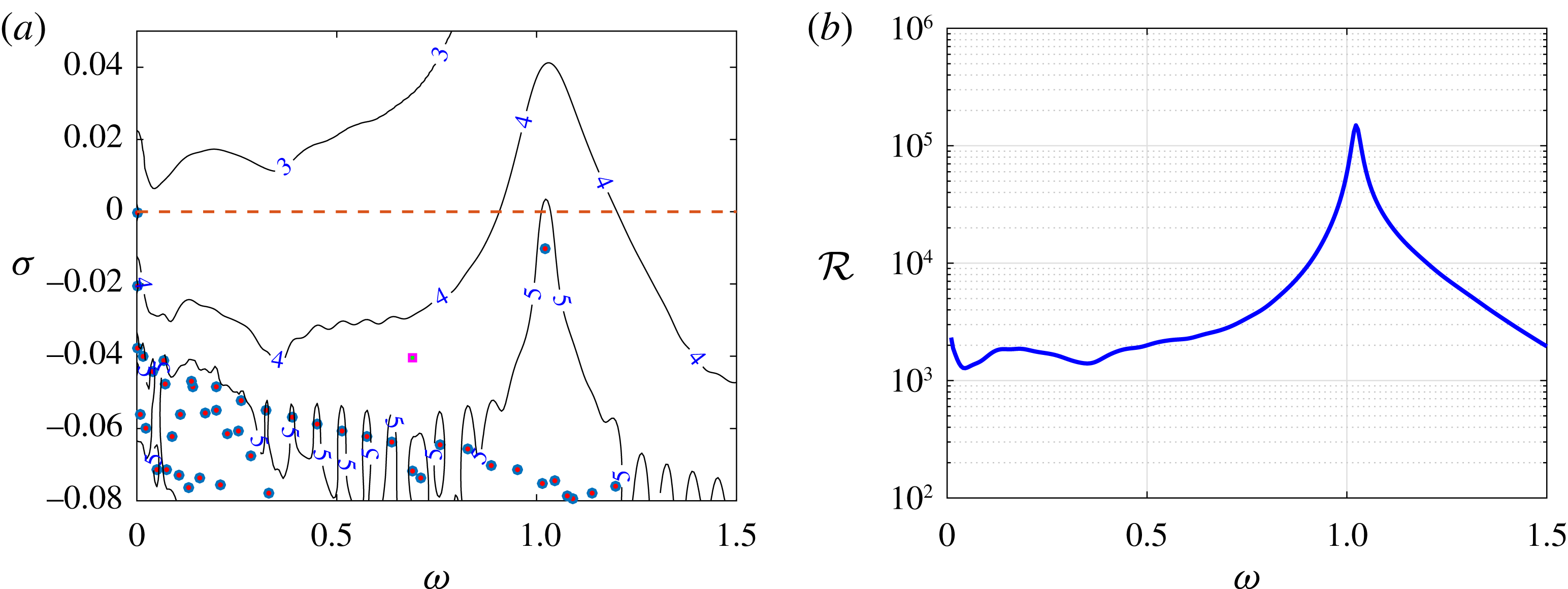
(a) Eigenspectrum (coloured symbols) and pseudospectrum (solid lines) of the linearized Navier–Stokes operator for
 $(\unicode[STIX]{x1D702},Re)=(1,700)$
. Circles (squares) represent varicose (sinuous) modes. The isolines represent pseudospectrum given by
 $\log _{10}\unicode[STIX]{x1D716}^{-1}$
contours, with
 $\unicode[STIX]{x1D716}$
ranging from
 $10^{-6}$
to
 $10^{-3}$
. (b) Approximation of the resolvent norm extracted from the pseudospectrum.

Regarding the
 $\unicode[STIX]{x1D702}=3$
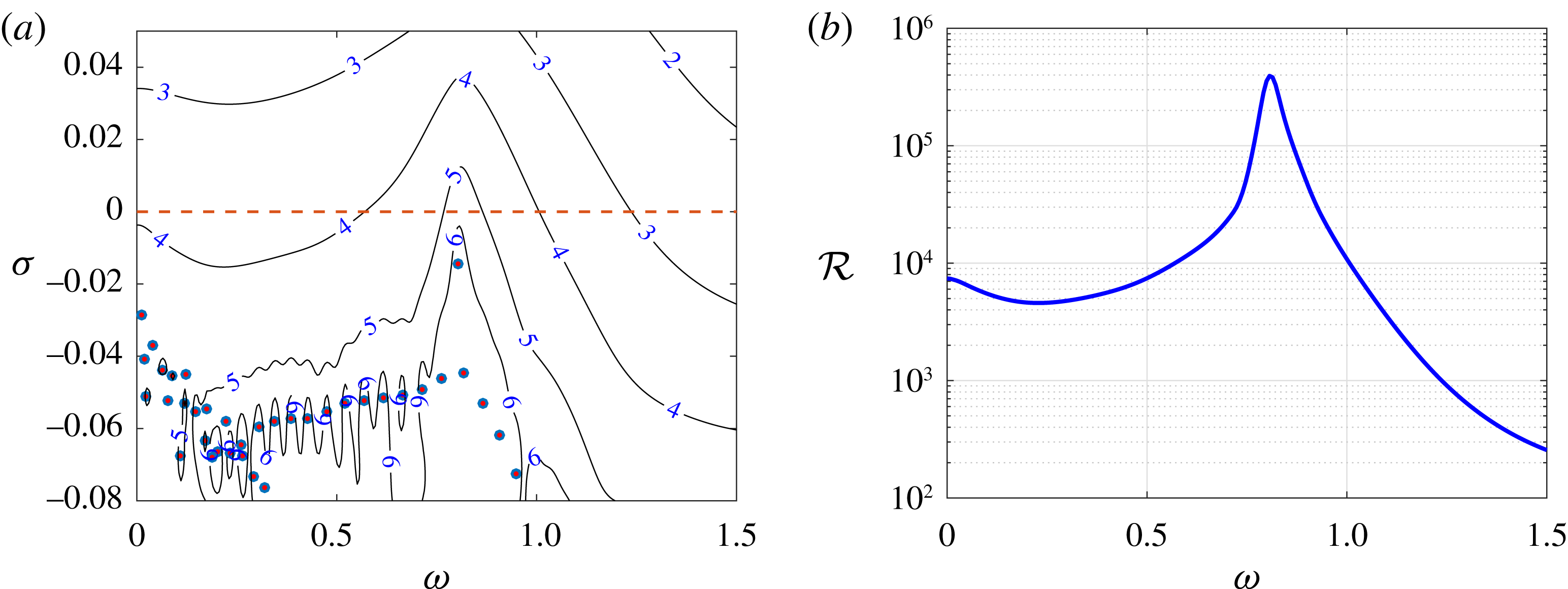
cases, only varicose modes are recovered in the spectra, as also found by Loiseau et al. (Reference Loiseau, Robinet, Cherubini and Leriche2014) for different values of the Reynolds number. Figure 8(a) provides the eigenspectrum (coloured symbols) for
 $Re=550$
, which is mostly made of stable modes with varicose symmetry. The least stable (isolated) mode oscillates at a circular frequency
 $\unicode[STIX]{x1D714}=0.8$
. The corresponding eigenvector is depicted in figure 11(a), showing a structure very similar to that of the least stable mode recovered for
 $\unicode[STIX]{x1D702}=1$
, although it has a longer extent in both the streamwise and spanwise directions. A similar structure also characterizes the corresponding isolated mode for
 $(\unicode[STIX]{x1D702},Re)=(3,500)$
(figure 9
a), despite having a smaller growth rate, while its circular frequency only slightly decreases (
 $\unicode[STIX]{x1D714}=0.77$
). In all of the cases considered herein, the dominant frequencies in the spectra as well as the main streamwise wavelength of the associated eigenvectors are very close to those measured experimentally (see table 1).
Same as in figure 8 for
 $(\unicode[STIX]{x1D702},Re)=(3,500)$
.

Same as in figure 8 for
 $(\unicode[STIX]{x1D702},Re)=(3,550)$
.

3.1.2 Pseudospectrum
For the range of parameters considered experimentally, all the modes in the spectrum are stable. Hence, the unsteadiness observed experimentally cannot be explained by a linear instability of the underlying base flow. It might however result from a large receptivity of the flow, which can be either linked to a strong transient growth of perturbations due to the non-orthogonality of the eigenvectors, or to a strong sensitivity of specific modes to external forcing. In the first case, the flow will act as an amplifier of a large range of frequencies, whereas in the latter case, it will ‘resonate’ at a precise frequency. To quantify the receptivity of the flow, the pseudospectrum of the linearized Navier–Stokes operator is evaluated using the Hessenberg matrix as in Toh & Trefethen (Reference Toh and Trefethen1996)
 $$\begin{eqnarray}\displaystyle \unicode[STIX]{x1D6EC}_{\unicode[STIX]{x1D716}}(\unicode[STIX]{x1D63C})=\{z\in \mathbb{C}:\Vert (z\,\unicode[STIX]{x1D644}-\unicode[STIX]{x1D63C})^{-1}\Vert >\unicode[STIX]{x1D716}^{-1}\}\approx \{z\in \mathbb{C}:\unicode[STIX]{x1D706}_{min}(z\unicode[STIX]{x1D644}-\log (\unicode[STIX]{x1D643})/\unicode[STIX]{x0394}t)<\unicode[STIX]{x1D716}\}, & & \displaystyle\end{eqnarray}$$
where the quantity
 $(z\unicode[STIX]{x1D644}-\unicode[STIX]{x1D63C})^{-1}$
is known as the resolvent of
 $\unicode[STIX]{x1D63C}$
(Trefethen & Embree Reference Trefethen and Embree2005), measuring how sensitive the eigenvalues of
 $\unicode[STIX]{x1D63C}$
are to some perturbations of
 $\unicode[STIX]{x1D63C}$
, and
 $\unicode[STIX]{x1D706}_{min}$
is the smallest singular value of a matrix, approximating its norm.
The pseudospectrum of
 $\unicode[STIX]{x1D63C}$
for
 $(\unicode[STIX]{x1D702},Re)=(1,700)$
is shown in figure 8(a). The solid lines depict the
 $\log _{10}(\unicode[STIX]{x1D716}^{-1})$
contours, representing the response of the system to a perturbation
 $z\unicode[STIX]{x1D644}$
. As can been seen, very high levels of
 $\log _{10}(\unicode[STIX]{x1D716}^{-1})$
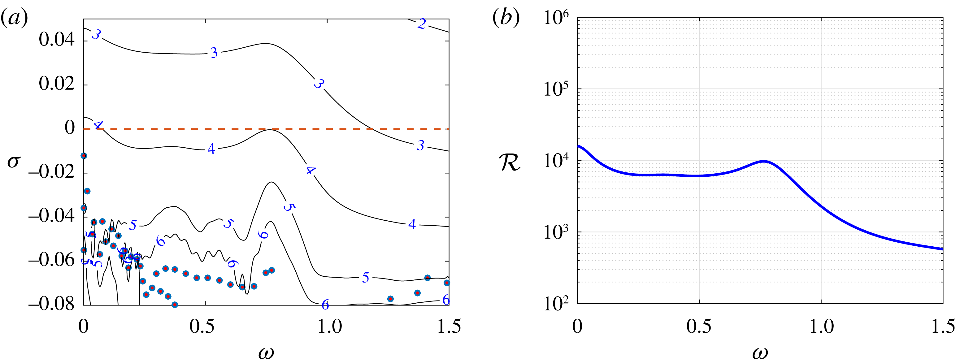
are reached in the vicinity of the eigenvalue associated with the varicose isolated mode, hence indicating that this particular eigenpair is highly sensitive to disturbances: even a disturbance as small as
 $\unicode[STIX]{x1D716}\approx 10^{-5}$
is sufficient to destabilize the system. Concerning the
 $\unicode[STIX]{x1D702}=3$
cases, the same comments can be made on the pseudospectrum obtained for
 $Re=550$
, shown in figure 10(a), whereas a slightly lower receptivity (
 $\unicode[STIX]{x1D716}\approx 10^{-4}$
) is found at
 $Re=500$
, the least stable eigenmode being farther from the real axis (see figure 9
a).
The isolated varicose modes being very sensitive no matter the case considered here, it is worth investigating how much its frequency, as well as other frequencies, can be amplified by the system. This can be easily evaluated from the pseudospectrum considering a purely imaginary perturbation
 $z$
and extracting the values of
 $\unicode[STIX]{x1D716}^{-1}$
along the
 $\unicode[STIX]{x1D70E}=0$
axis, thus providing a proxy for the resolvent norm. Figure 8(b) shows the amplification factor of purely imaginary forcing at different frequencies found using (3.5), for the case
 $(\unicode[STIX]{x1D702},Re)=(1,700)$
. The maximum gain is reached for
 $\unicode[STIX]{x1D714}=1.02$
, i.e. the circular frequency of the isolated varicose mode, very close to that measured experimentally. Moreover, the associated gain is very high (
 ${\approx}10^{5}$
), indicating that the energy of the response to a harmonic forcing at
 $\unicode[STIX]{x1D714}=1.02$
can be amplified by up to 5 orders of magnitude. A similar value of the gain (
 ${\approx}1.4\times 10^{5}$
) can be obtained by forcing a linear numerical simulation using the adjoint counterpart of the varicose mode with its associated frequency and marching it to long times, allowing the establishment of an asymptotical behaviour. The isolated varicose mode thus appears to be almost orthogonal to the other modes of the eigenspectrum, strongly suggesting that, in the case considered herein, non-normality of the linearized Navier–Stokes operator does not play a significant role. Similar conclusions can be drawn for the
 $\unicode[STIX]{x1D702}=3$
cases. Figure 10(b) shows the amplification factor of purely imaginary forcing for the case at
 $Re=550$
, which has a strong peak (
 ${\approx}393~400$
) at
 $\unicode[STIX]{x1D714}=0.8$
, the circular frequency of the isolated varicose mode. The same can be said about the case at
 $Re=500$
depicted in figure 9(b), although the peak associated with the isolated mode is no longer the global maximum of the amplification curve and is less pronounced (
 $O(10^{4})$
) with respect to the previous cases, the global isolated mode being more stable.
3.1.3 Optimal forcing and response
The previous analysis has shown that a small perturbation is sufficient to make the system resonate at the circular frequency of the varicose isolated mode. It provides however no information regarding the spatial evolution of the perturbations induced by this quasi-resonance phenomenon. To gain some insights, we investigate which kind of harmonic forcing, characterized by the frequency of the global isolated mode, is able to induce the largest possible response. Towards this aim, a forcing is introduced in the linearized Navier–Stokes equations such that
 $$\begin{eqnarray}\displaystyle \frac{\unicode[STIX]{x2202}\boldsymbol{u}}{\unicode[STIX]{x2202}t}=\unicode[STIX]{x1D63C}\boldsymbol{u}+\boldsymbol{f}. & & \displaystyle\end{eqnarray}$$
Assuming a periodic forcing
 $\boldsymbol{f}(\boldsymbol{x},t)=\hat{\boldsymbol{f}}(\boldsymbol{x})\text{e}^{\text{i}\unicode[STIX]{x1D714}t}+\text{c.c.}$
, the response of the system takes the form
 $\boldsymbol{u}(\boldsymbol{x},t)=\hat{\boldsymbol{u}}(\boldsymbol{x})\text{e}^{\text{i}\unicode[STIX]{x1D714}t}+\text{c.c}$
. Introducing this ansatz in (3.6), the relation between
 $\hat{\boldsymbol{f}}$
and
 $\hat{\boldsymbol{u}}$
is given by
 $$\begin{eqnarray}\displaystyle \hat{\boldsymbol{u}}=(\text{i}\unicode[STIX]{x1D714}\unicode[STIX]{x1D644}-\unicode[STIX]{x1D63C})^{-1}\hat{\boldsymbol{f}}, & & \displaystyle\end{eqnarray}$$
where the resolvent
 $(\text{i}\unicode[STIX]{x1D714}\unicode[STIX]{x1D644}-\unicode[STIX]{x1D63C})^{-1}$
has the role of a transfer function between the harmonic forcing
 $\hat{\boldsymbol{f}}$
and the asymptotic response
 $\hat{\boldsymbol{u}}$
. In order to find the forcing field at a given frequency
 $\unicode[STIX]{x1D714}$
maximizing the response of the system, the quantity
 $$\begin{eqnarray}\displaystyle {\mathcal{R}}(\unicode[STIX]{x1D714})=\max _{\boldsymbol{f}}\frac{\Vert (\text{i}\unicode[STIX]{x1D714}\unicode[STIX]{x1D644}-\unicode[STIX]{x1D63C})^{-1}\boldsymbol{f}\Vert }{\Vert \,\boldsymbol{f}\Vert }=\Vert (\text{i}\unicode[STIX]{x1D714}\unicode[STIX]{x1D644}-\unicode[STIX]{x1D63C})^{-1}\Vert & & \displaystyle\end{eqnarray}$$
has to be optimized. The solution to this convex optimization problem is found iteratively by a direct-adjoint loop (Monokrousos et al. Reference Monokrousos, Åkervik, Brandt and Henningson2010) which has been implemented in the Nek5000 code. For more details about the resolvent analysis, the reader is refereed to Schmid (Reference Schmid2007), while Luchini & Bottaro (Reference Luchini and Bottaro2014) provide a detailed explanation of the derivation of the adjoint Navier–Stokes equations and their use in fluid mechanics.
The shapes of the optimal forcing and response at
 $\unicode[STIX]{x1D714}=1.02$
for the case
 $(\unicode[STIX]{x1D702},Re)=(1,700)$
are shown in figure 12(a and b, respectively). The optimal forcing is constituted by streamwise-alternated patches of velocity perturbations, placed upstream of the cylinder. Remarkably, it shows a varicose symmetry, similarly to the most sensitive isolated mode previously analysed. As might be expected, the shape of the optimal response induced by such a forcing is very close to the shape of the isolated varicose mode, as one can observe by comparing figure 12(b) to figure 7(a). Again, this behaviour can be ascribed to the quasi-orthogonality of the varicose mode with respect to the other modes. Note finally that the optimal gain
 ${\mathcal{R}}(\unicode[STIX]{x1D714})=149\,170$
is in good agreement with the estimate obtained from the pseudospectrum analysis in § 3.1.2.
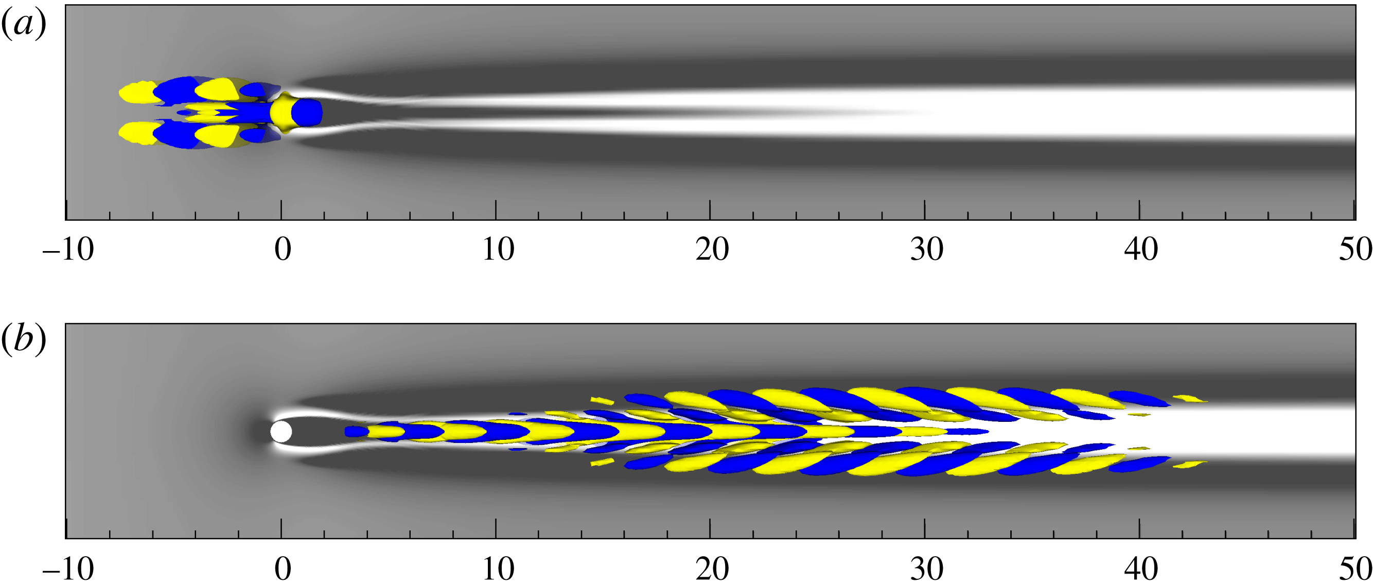
The optimal forcing and response at
 $\unicode[STIX]{x1D714}=0.8$
are provided in figure 13(a and b, respectively) for the case
 $(\unicode[STIX]{x1D702},Re)=(3,550)$
. As before, the shape of the optimal response (forcing) almost coincides with the shape of the isolated (adjoint) varicose mode, as one can infer when comparing figures 11 and 13. Despite the linearly stable nature of the underlying base flows, these observations strongly suggest that the unsteadiness observed experimentally results from a quasi-resonance of the least stable varicose eigenmode due to the external forcing inherent to an experimental facility.
(a) Eigenvector associated with isolated varicose mode, and (b) its adjoint counterpart for case
 $(\unicode[STIX]{x1D702},Re)=(3,550)$
. Grey scales and isosurfaces are the same as in figure 7.

Shape of (a) the optimal forcing and (b) the optimal response for the case
 $(\unicode[STIX]{x1D702},Re)=(1,700)$
. Grey scales and isosurfaces are the same as in figure 7.

Shape of (a) the optimal forcing and (b) the optimal response for case
 $(\unicode[STIX]{x1D702},Re)=(3,550)$
. Grey scales and isosurfaces are the same as in figure 7.

3.2 Nonlinear analysis
The different analyses presented in § 3.1 have demonstrated how sensitive the flow is despite its linearly stable nature. More specifically, the pseudospectrum analysis (§ 3.1.2) and the optimal forcing analysis (§ 3.1.3) have strongly underlined the receptivity of the flow at the frequency of the least stable varicose eigenmode and its quasi-resonant response. Despite their success, these analyses rely on the linearized Navier–Stokes equations and, as such, do not provide any insight into the nonlinear evolution of the perturbation. In order to properly quantify this response, one would need to perform a nonlinear resolvent analysis. Such an analysis is however beyond the scope of our current capabilities. One can nonetheless gain some insights into the nonlinear evolution of the perturbation by means of direct numerical simulations. For that purpose, two different types of direct numerical simulations are considered hereafter:
-
(i) an impulse-response direct numerical simulation;
-
(ii) direct numerical simulations forced by the optimal forcing obtained from the resolvent analysis with three different amplitudes.
Regarding the boundary conditions, a Blasius velocity profile is now prescribed at the inflow boundary while a classical outflow condition is used at the other end of the domain. Note furthermore that the fringe regions included in the linear analyses are no longer used.
3.2.1 Impulsively forced DNS
The pseudospectrum and optimal forcing analyses provided in the previous sections suggest that the flow can be highly receptive at the frequency of the isolated global mode. Thus, even a direct numerical simulation initialized by a generic perturbation can be expected to give rise to a response dominated by the frequency of that mode, as observed in the experiments presented in § 2.2. To ascertain this hypothesis, we focus our attention on the case
 $(\unicode[STIX]{x1D702},Re)=(1,700)$
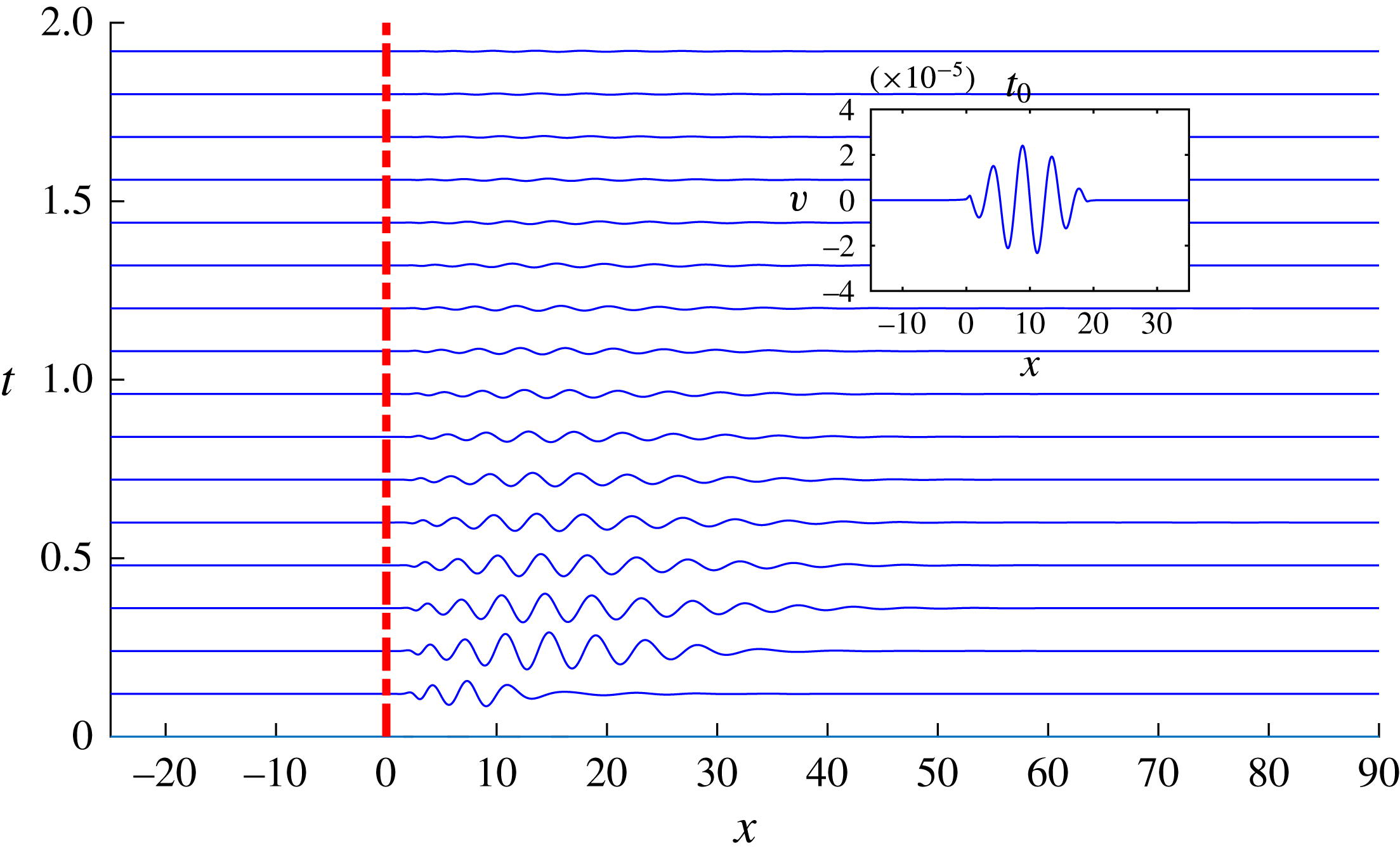
and perform a DNS initialized by a superimposition of the linearly stable base flow and of an impulsive wavepacket of the form
 $v(x,0)=\sin (\unicode[STIX]{x03C0}x/5)\sin (\unicode[STIX]{x03C0}x/20)$
, shown in the inset of figure 14. The wavepacket, placed downstream of the cylinder in the region
 $0<x<20$
, has an initial amplitude
 $A=5\times 10^{-5}$
, which is sufficiently low to allow a (mostly) linear evolution of the flow response. The main frame of figure 14 provides a space–time diagram showing the evolution of the wavepacket. It is initially amplified and stretched in the streamwise direction up to
 $x\approx 40$
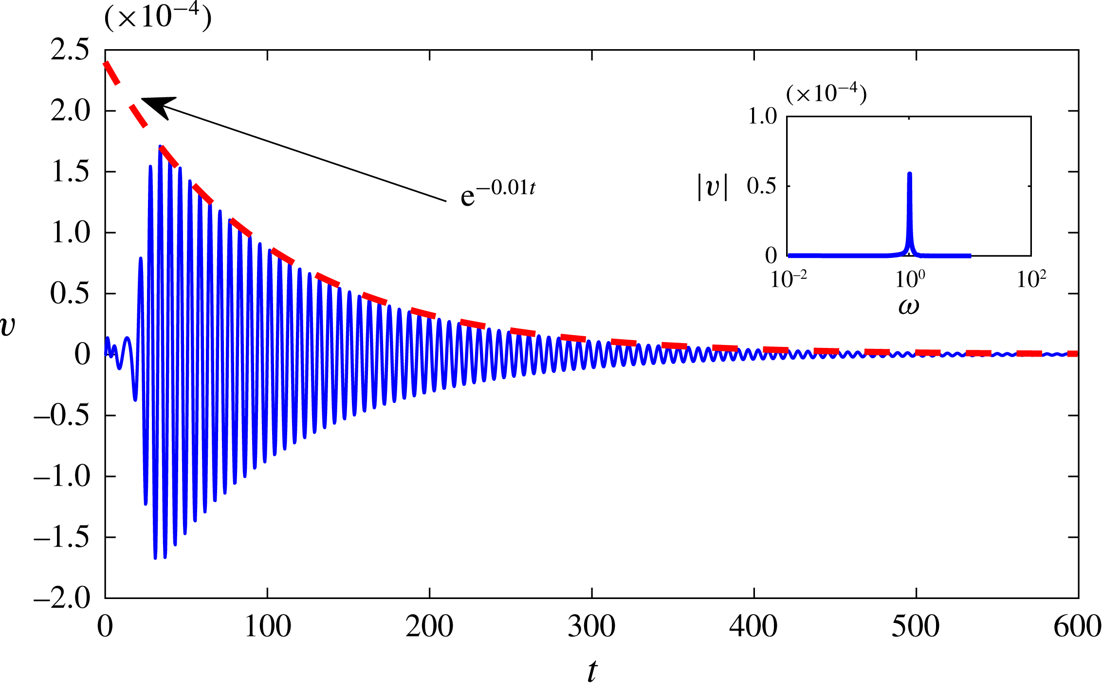
. After its initial transient growth, the wavepacket begins to decrease its amplitude and streamwise extent, slowly fading away as time is increased, as it might have been anticipated by the initial low amplitude of the wavepacket and linearly stable nature of the flow. Figure 15 provides the time trace of the perturbation’s vertical velocity component monitored by a probe located at
 $(x,y,z)=(10,1.2,0)$
. After a relatively short transient, the signal oscillates at a preferential frequency, followed by an exponential decay. This decay is well approximated by an exponential function characterized by a decay rate
 $-0.01$
in close agreement with the decay rate of the isolated varicose mode (see figure 8
a). Moreover, a Fourier transform of that signal highlights the existence of a dominant peak at
 $\unicode[STIX]{x1D714}=1.02$
, demonstrating that the most unstable mode of the spectrum can indeed be triggered by a generic perturbation injected impulsively into the flow.
Time evolution of the wall-normal velocity perturbation
 $v$
measured at
 $(y,z)=(1.2,0)$
for the impulsively perturbed DNS. The inset provides the shape of the wall-normal perturbation added to the base flow at
 $t=0$
. The red dashed line indicates the cylinder position. The case considered is
 $(\unicode[STIX]{x1D702},Re)=(1,700)$
.

Time evolution of the wall-normal velocity perturbation
 $v$
extracted at
 $(x,y,z)=(10,1.2,0)$
. The inset shows the Fourier transform of that time signal, showing that the response of the flow to a generic perturbation is indeed dominated by the most receptive global mode
 $(\unicode[STIX]{x1D70E},\unicode[STIX]{x1D714})=(-0.01,1.02)$
. The case considered is
 $(\unicode[STIX]{x1D702},Re)=(1,700)$
.

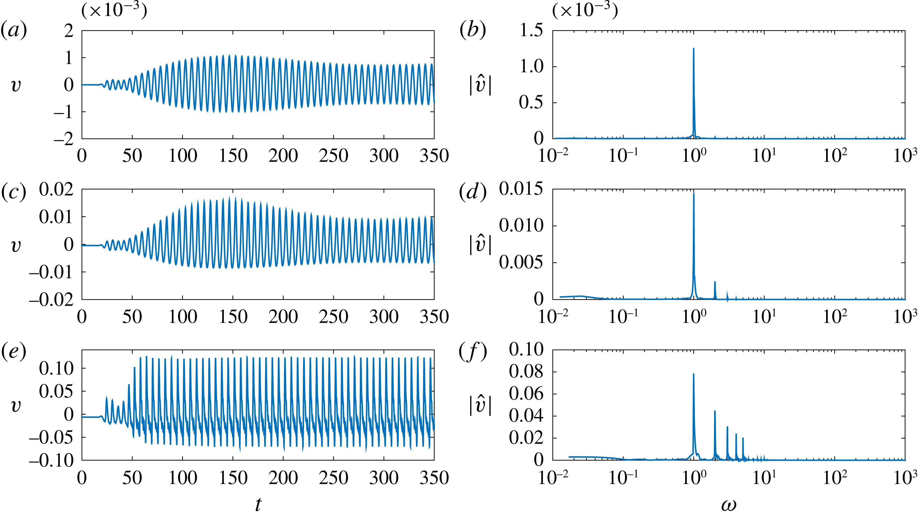
(a,c,e) Time evolution of the wall-normal velocity fluctuation for initial amplitudes
 $A=1\times 10^{-5}$
(a,b),
 $A=1\times 10^{-4}$
(c,d) and
 $A=1\times 10^{-3}$
(e,f) and related Fourier transform (b,d,f). The case considered is
 $(\unicode[STIX]{x1D702},Re)=(1,700)$
.

3.2.2 Optimally forced DNS
Once ascertained that the dominant frequencies observed within the flow are likely to result from a quasi-resonance of the isolated varicose mode, it is interesting to shed light onto the transition scenario induced by this phenomenon, with the final aim of comparing the generated coherent structures with those observed experimentally. We thus focus once again on the case
 $(\unicode[STIX]{x1D702},Re)=(1,700)$
, using the optimal forcing at
 $\unicode[STIX]{x1D714}=1.02$
to force a DNS. The optimal forcing is scaled with three different initial amplitudes (
 $A=10^{-5}$
,
 $10^{-4}$
, and
 $10^{-3}$
) in order to investigate the effect of nonlinearity on the time evolution of the flow. The resulting wall-normal velocity fluctuations, given by the instantaneous velocity minus its temporal mean value, are monitored by a probe located at
 $(x,y,z)=(10,1.5,0)$
. The time traces (a,c,e) obtained for the three amplitudes considered and their frequency spectra (b,d,f) are provided in figure 16.
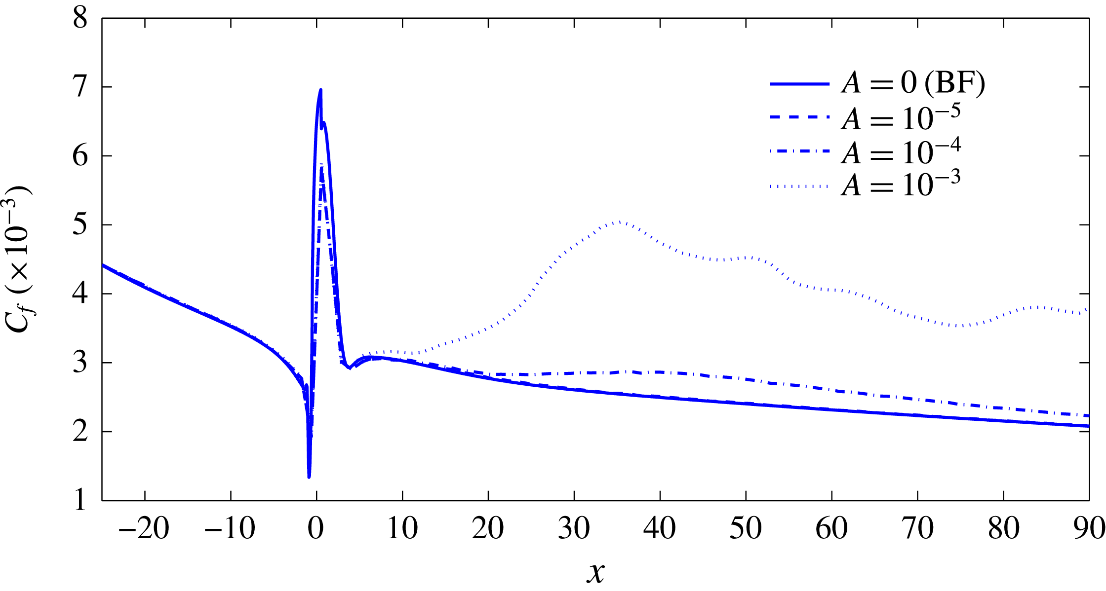
Streamwise evolution of the skin friction factor
 $C_{f}(x)$
for four different amplitudes of the optimal forcing. The case considered is
 $(\unicode[STIX]{x1D702},Re)=(1,700)$
.

For the lowest amplitude (a,b), a time-periodic behaviour appears to settle after a short initial phase characterized by a transient growth of the perturbation. After this initial phase, a periodic signal with associated circular frequency equal to that of the varicose mode is observed. Increasing the amplitude of the forcing begins to trigger the nonlinearities, hence resulting in the emergence of smaller-amplitude harmonics which rapidly fade away leading, again, to the establishment of a quasi-periodic signal (figure 16 c,d). For the largest amplitude considered herein, an even larger number of harmonics are generated by the nonlinearities, inducing a saturation of the signal amplitude as shown in figure 16(e,f).
In order to obtain a quantitative criterion defining whether transition to turbulence has occurred or not, the skin friction coefficient
 $C_{f}(x)$
is computed. Figure 17 depicts the streamwise evolution of
 $C_{f}(x)$
for the optimally forced DNS at the three amplitudes considered. Note that the evolution of
 $C_{f}(x)$
for the unperturbed steady base flow is also reported for the sake of reference. For the lowest value of the forcing amplitude, the flow remains laminar behind the roughness, as indicated by the
 $C_{f}$
curve which is superimposed to that of the base flow (compare the dashed and the solid lines). For
 $A=10^{-4}$
, the skin friction begins to deviate from the reference state, while for
 $A=10^{-3}$
, it strongly increases. Such an increase of the skin friction typically indicates the onset of transition towards a turbulent flow, although the values of
 $C_{f}$
typical of high Reynolds number turbulent boundary-layer flows have not been reached yet in the computational domain considered.
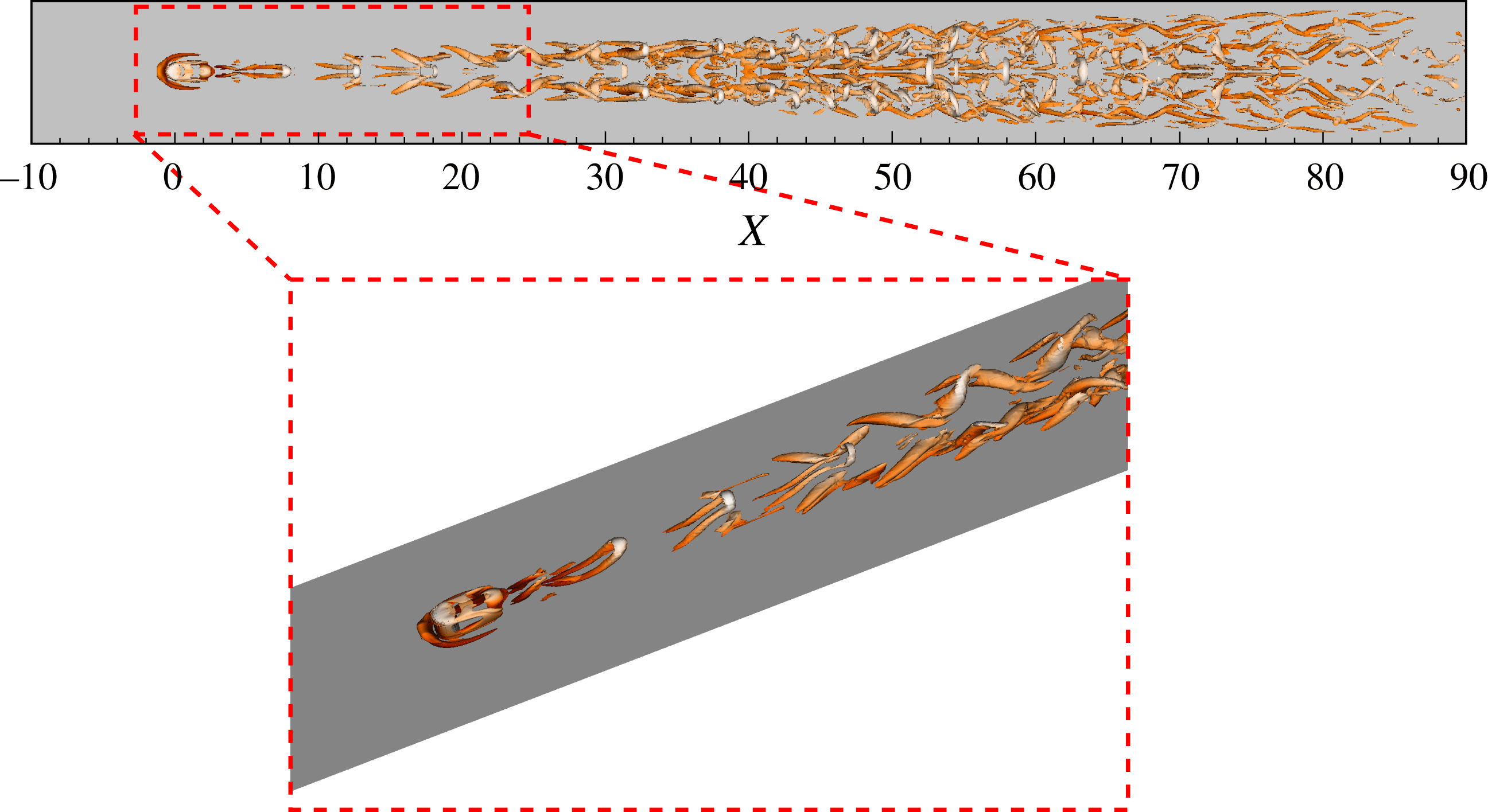
Hairpin vortices highlighted by lambda-2 criterion as defined by Jeong & Hussain (Reference Jeong and Hussain1995) (
 $\unicode[STIX]{x1D706}_{2}=-0.02$
) and coloured by streamwise velocity. The case considered is
 $(\unicode[STIX]{x1D702},Re)=(1,700)$
.

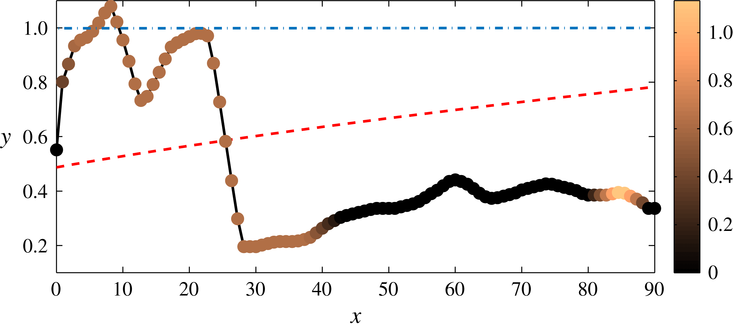
Variation in the streamwise direction of the wall-normal position of the maximum amplitude mode of the spanwise Fourier transform of the
 $u_{rms}$
. Colour bar indicates the spanwise wavenumber of the dominant Fourier mode. Red dashed line provides the analytical displacement thickness of the Blasius solution whereas the blue dashed-dotted line indicates the height of the cylinder. The case considered is
 $(\unicode[STIX]{x1D702},Re)=(1,700)$
.

Figure 18 provides a snapshot of the instantaneous flow where the vortical structures are highlighted using the
 $\unicode[STIX]{x1D706}_{2}$
criterion (Jeong & Hussain Reference Jeong and Hussain1995). One can observe the generation of hairpin vortices right downstream of the roughness element, the first one being placed at
 $x\approx 2$
. Up to
 $x\approx 30$
, a train of hairpin vortices can be observed, whose heads appear to have a streamwise spacing of
 $\unicode[STIX]{x0394}x\approx 4.7$
. The vortical structures also spread in the spanwise direction generating
 $\unicode[STIX]{x1D6EC}$
vortices at their spanwise sides. These primary hairpin vortices then start to break down at
 $x\approx 30$
, corresponding to the streamwise position at which the skin friction
 $C_{f}$
reaches its highest value. This transition scenario closely resembles the one observed experimentally, showing the shedding of hairpin vortices having a varicose symmetry with streamwise wavelength
 ${\approx}5$
. However, due to the nature of the optimal forcing, the flow remains symmetric up to the end of the domain (see figure 18) and the associated spatial and temporal Fourier spectra remain characterized by a limited number of different wavelengths.
Finally, to further characterize the spatial spreading of the fluctuation, a spanwise Fourier transform of the
 $u_{rms}$
field for different selected
 $y$
and
 $x$
positions has been performed. The wall-normal position of the dominant Fourier mode in the
 $y$
-direction for a fixed
 $x$
position (circles) and the associated spanwise wavenumber (colours of the circles as specified by the colour bar) are shown in figure 19. The first peak (
 $x=9$
) is associated with the generation of the train of hairpin vortices behind the cylinder, the corresponding spanwise wavelength,
 $\unicode[STIX]{x1D6FD}=0.63$
, being close to the spanwise dimension of the first hairpin. For
 $x\geqslant 10$
, the first hairpin vortex starts to disappear, whereas a second one is generated downstream, inducing a second peak at
 $x=23$
due to the growth of a second perturbation that wraps the two low streaks. For
 $x>26$
, the wall-normal position of the dominant Fourier mode of
 $u_{rms}$
rapidly moves towards the wall, where the flow starts to become turbulent (see figure 17). Further downstream, the maximum amplitude of the Fourier transform is characterized by
 $\unicode[STIX]{x1D6FD}=0$
, but, due to the spanwise symmetry of the flow field, a second peak at
 $\unicode[STIX]{x1D6FD}=1.26$
is observed, which becomes predominant for
 $85\leqslant x\leqslant 90$
.
4 Summary and conclusions
Following the work of Loiseau et al. (Reference Loiseau, Robinet, Cherubini and Leriche2014), the properties of the incompressible flow induced by three-dimensional cylindrical roughness elements of various aspect ratios have been studied by the joint use of experimental investigations, linear stability analyses, direct numerical simulations and optimal forcing analysis. Despite the linearly stable nature of the base flows (§ 3.1.1) for the range of parameters considered herein, the experiments conducted in the Laminarwasserkanal at IAG have highlighted the quasi-periodic shedding of hairpin vortices downstream of the roughness elements (§ 2.2).
In all cases considered, counter-rotating pairs of horseshoe vortices wrapped around the roughness element are created by the impinging boundary layer. Further downstream, the legs of these horseshoe vortices create several high- and low-speed streamwise streaks due to the lift-up effect. As shown by Loiseau et al. (Reference Loiseau, Robinet, Cherubini and Leriche2014), the properties of these streaks are crucial for the streamwise development of the global instability stemming from the near wake of the roughness element. In the present work however, the unsteadiness observed in the experiments cannot be explained by the existence of a linearly unstable eigenmode for the range of parameters considered herein. A pseudospectrum analysis has nonetheless revealed the high sensitivity to external disturbances of the least stable varicose eigenmode whose frequency closely matches the frequency measured experimentally. Depending on the exact case considered, disturbances at the frequency of this isolated varicose eigenmode can be amplified by four to six orders of magnitude. The shape of the optimal forcing and associated response at this particular frequency have been obtained by means of a fully three-dimensional resolvent analysis. Surprisingly, the optimal forcing closely resembles the isolated adjoint varicose eigenmode while the associated response is almost indistinguishable from the direct eigenmode. Such a resemblance between the optimal forcing (response) and the adjoint (direct) eigenmode and the good agreement between the most amplified frequency and the one observed experimentally strongly suggests that the unsteadiness observed experimentally results from a quasi-resonance of the least stable varicose eigenmode rather than being due to the non-normality of the linearized Navier–Stokes operator.
Although the analyses presented herein have provided a relatively simple explanation of the origin of unsteadiness in the experiment, it has to be noted that we have considered only a small portion of the parameter space. The influence of the shape of the roughness element, its aspect ratio, as well as the boundary-layer thickness of the incoming flow on the properties (frequency, symmetry) of the resonant mode still need to be determined. With the aim of determining the lower bound for transition in the von Doenhoff–Braslow diagram, direct numerical simulations in the presence of free-stream turbulence might also be a valuable tool to investigate the receptivity of the flow in more realistic conditions.
4.1 Concluding remarks
In their original work Loiseau et al. (Reference Loiseau, Robinet, Cherubini and Leriche2014) have shown that the upper bound for transition in the von Doenhoff–Braslow diagram could potentially be explained by a global instability of the underlying base flows. Their attention has however been mostly focused on the
 $\unicode[STIX]{x1D702}=1$
roughness element and the evolution of the sinuous global instability it experiences due to a supercritical Hopf bifurcation, leaving two questions unanswered:
-
(i) What is the nature of the bifurcation giving rise to a linearly unstable varicose eigenmode?
-
(ii) Can these flows experience subcritical transition to turbulence, thus providing an explanation for the lower bound for transition in the von Doenhoff–Braslow diagram?
Although this work does not provide a definite answer to the first question, the direct numerical simulations (§ 3.2) clearly demonstrate that subcritical transition can indeed be induced by a relatively small external forcing. While the characteristics of the unsteadiness in case of a subcritical transition to turbulence usually differs quite significantly from the spectral properties of the linearized Navier–Stokes operator in most wall-bounded shear flows, it is surprising that, herein, these characteristics are well predicted by the simple use of linear stability and pseudospectrum analyses. In particular, the pseudospectrum analysis can provide approximations of the lower bound for transition as it estimates the required amplitude of an external forcing in order to trigger the resonant mode. In the present case, a disturbance of order
 $10^{-3}$
is found sufficient for initiating the quasi-resonance phenomenon leading to transition. This order of magnitude is similar to the turbulence intensity measured in the water channel. Such an observation might greatly reduce the computational burden of investigating the properties of roughness-induced transition, even when a turbulent mean flow is taken as the base flow as it would require only a limited number of stability and pseudospectra analyses. Note that it is still unclear at present time whether this observation remains true for all flows induced by a fully three-dimensional geometry. One may however hypothesize that it remains valid if the leading isolated modes are almost orthogonal to the rest of the eigenmodes.
Acknowledgements
Part of this work was performed using HPC resources from GENCI-[CCRT/CINES/IDRIS] (grant x20162a6362). The experimental part of this work was financially supported by the Deutsche Forschungsgemeinschaft (DFG) under reference number RI 680/32-1.
Appendix A. Grid convergence study
Within the spectral elements framework, two types of grid refinement can be undertaken:
-
(i)
 $h$
-type: keep the number of spectral element constant and increase the order of the Lagrange interpolants;
-
(ii)
$p$
-type: keep the order of the Lagrange interpolants constant and increase the number of spectral elements used.


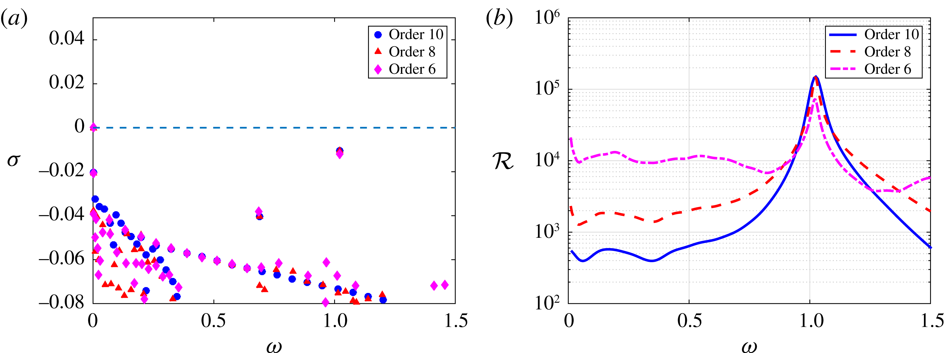
In the present work, the grid convergence analysis has been performed using a
 $h$
-type refinement due to its simplicity. Figure 20(a) depicts the eigenspectrum of the linearized Navier–Stokes operator for the case
 $(\unicode[STIX]{x1D702},Re)=(1,700)$
for three different polynomial orders, namely
 $N=6$
, 8 and 10. For the present configuration, the spectral element mesh is kept constant and is made of
 $23\,544$
elements (figure 21 depicts the coarse grid distribution of the spectral elements in a given horizontal plane). As shown, the eigenvalues of interest are hardly influenced by the mesh refinement. On the other hand, figure 20(b) depicts the approximation of the resolvent norm
 ${\mathcal{R}}(\unicode[STIX]{x1D714})$
as obtained by the pseudospectrum analysis. Although the peak frequency and gain do not seem to be greatly influenced by the polynomial order of the Lagrange interpolants used, the low-frequency part of this resolvent (i.e.
 $\unicode[STIX]{x1D714}<0.75$
) appears to be significantly stabilized as the polynomial order is increased. Similar observations have been made for other aspect ratio cases. In all of this work, the results presented have been obtained with a polynomial degree
 $N=8$
.
Grid convergence analysis for the case
 $(\unicode[STIX]{x1D702},Re)=(1,700)$
. (a) Evolution of the linearized Navier–Stokes operator as the degree of the Lagrange interpolants is increased from
 $N=6$
up to
 $N=10$
. (b) Same as (a) for the approximation of the resolvent norm based on the pseudospectrum analysis.

Coarse grid distribution of the spectral elements in a given horizontal plane for the aspect ratio
 $\unicode[STIX]{x1D702}=1$
case. Note that in the simulation
 $N$
Lagrange interpolants are used in the three directions of space within each of these elements.

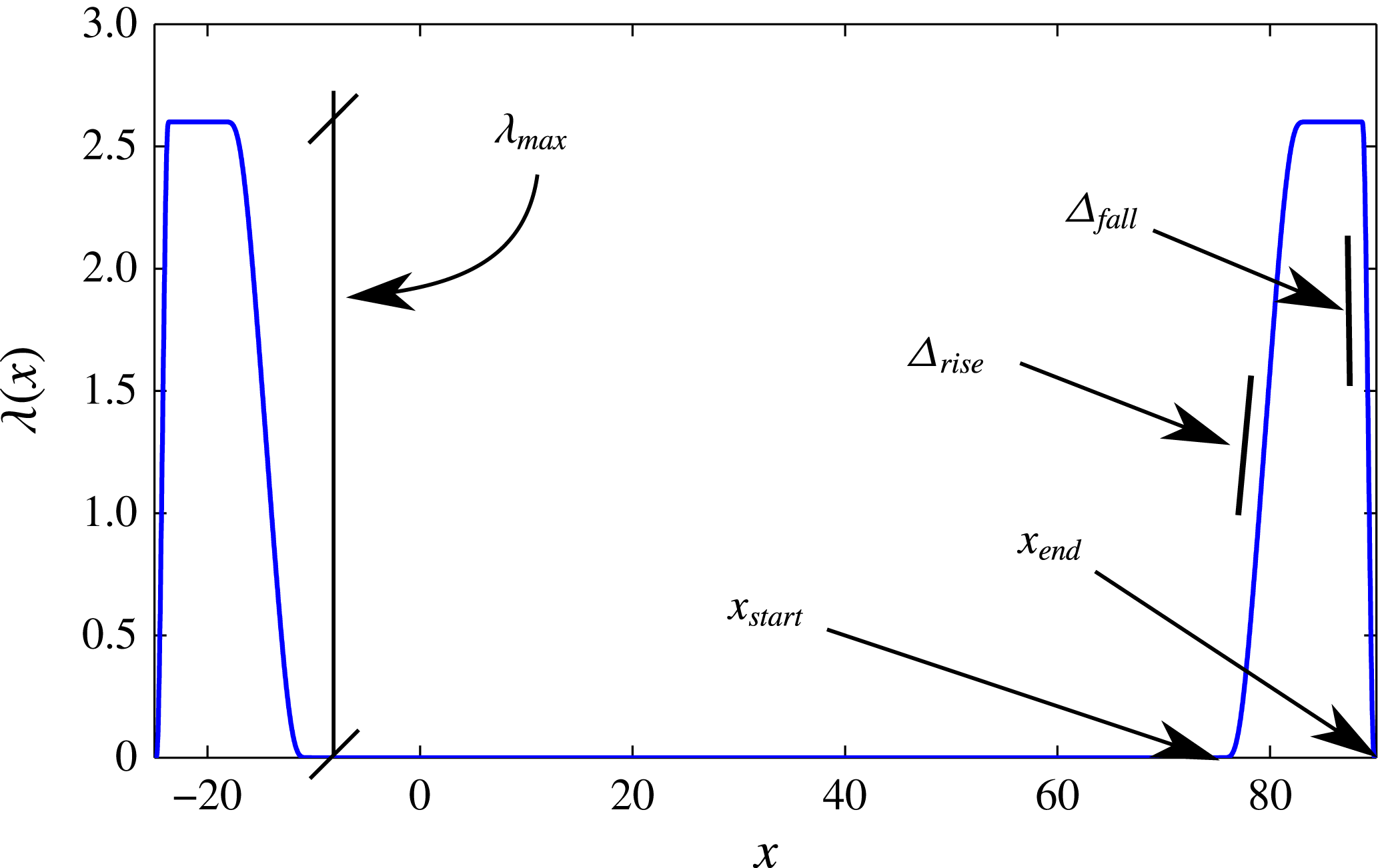
Appendix B. Fringe regions
The use of a fringe region was deemed necessary for the calculation of the optimal forcing and optimal response using the direct-adjoint looping procedure described in Monokrousos et al. (Reference Monokrousos, Åkervik, Brandt and Henningson2010). For that purpose, a force is added in the momentum equations, given by
 $$\begin{eqnarray}\displaystyle \boldsymbol{F}(\boldsymbol{x})=-\unicode[STIX]{x1D706}(x)\boldsymbol{u}(\boldsymbol{x}), & & \displaystyle\end{eqnarray}$$
where
 $\boldsymbol{u}$
is the perturbation velocity field and
 $\unicode[STIX]{x1D706}(x)$
is a streamwise-dependent non-negative fringe function. This force is applied in the region
 $[x_{start};x_{end}]=[75;90]$
and is given by
 $$\begin{eqnarray}\displaystyle \unicode[STIX]{x1D706}(x)=\unicode[STIX]{x1D706}_{max}\left[S\left(\frac{x-x_{start}}{\unicode[STIX]{x1D6E5}_{rise}}\right)-S\left(\frac{x-x_{end}}{\unicode[STIX]{x1D6E5}_{fall}}+1\right)\right], & & \displaystyle\end{eqnarray}$$
where
 $S(x)$
is a regularized step function defined as
 $$\begin{eqnarray}\displaystyle S(x)=\left\{\begin{array}{@{}ll@{}}0, & x\leqslant 0,\\ 1/[1+\exp (1/(x-1)+1/x)], & 0<x<1,\\ 1, & x\geqslant 0,\end{array}\right. & & \displaystyle\end{eqnarray}$$
with
 $\unicode[STIX]{x1D706}_{max}=2.6$
,
 $\unicode[STIX]{x1D6E5}_{rise}=60\,\%$
,
 $\unicode[STIX]{x1D6E5}_{fall}=10\,\%$
. See Lundbladh et al. (Reference Lundbladh, Berlin, Skote, Hildings, Choi, Kim and Henningson1999) for an investigation on how the fringe parameters affect the disturbance in the fringe. The influence of this zone has been verified, and its location and characteristics have been chosen so as not to have any significant influence on the results. Note finally that, for the adjoint simulations, a similar fringe zone is also used upstream of the roughness element, between
 $[x_{start};x_{end}]=[-25;10]$
. Figure 22 depicts the spatial extent of the fringe region as well as summarizing the different numerical parameters.
Visualization of the
 $\unicode[STIX]{x1D706}(x)$
function and relevant parameters in the fringe region.