1. INTRODUCTION
A typical Strapdown Inertial Navigation System (SINS) algorithm is a process of calculating the attitude/velocity/position in the navigation frame by integration of the angular rate and total acceleration. Total acceleration is calculated as the sum of gravitational acceleration and specific force acceleration which is produced by non-gravitational forces. Modern attitude integration adopts a two-speed approach: a high-speed calculation where an exact rotation vector differential equation is integrated to account for the non-commutative errors caused by multi-axis angular motion and a moderate-speed calculation in which an analytically exact equation is used to map the rotation vector (provided from the high-speed integration) to attitude changes. A two-speed approach can be also used for velocity/position integration in dynamic environments that parallel the two-speed attitude integration approach. The high speed velocity/position algorithms are designed to account for errors caused by angular and linear oscillation (Savage, Reference Savage1998b), and the moderate algorithms are used to update velocity/position. Thus, the navigation algorithms are divided into two parts: high-speed circle and moderate-speed circle.
However, unlike the attitude algorithm which utilises a rotation vector to measure the exact attitude change, velocity/position integration algorithms lack a parallel exact analytical formula, thus being typically limited to first-order accuracy under manoeuvring conditions (Savage, Reference Savage1998b). To overcome the limitation, Wu et al. (Reference Wu, Hu, Hu, Li and Lian2005) developed the Dual Quaternion (DQ) algorithm which combined rotation and translation as a whole. The geometry algebra INS algorithm (Wu and Wang, Reference Wu and Wang2012) is similar to the DQ algorithm. Later, Savage (Reference Savage2006b) proposed the Velocity Translation Vector (VTV) and Position Translation Vector (PTV) which achieved exact solutions to rigid body translation. Comparisons between DQ and VTV show that dual quaternion has the same velocity translation part as Savage's VTV (Wu, Reference Wu2006). For the position translation part, Savage's PTV can be reduced to the double integral of specific force acceleration when angular-rate/specific-force are constant, while the DQ deduced PTV has no such character (Wu and Xiao, Reference Wu and Xiao2011; Savage, Reference Savage2006a).
For all the algorithms presented (Savage, Reference Savage1998a; Savage, Reference Savage1998b; Savage, Reference Savage2006b; Wu et al., Reference Wu, Hu, Hu, Li and Lian2005; Wu and Wang, Reference Wu and Wang2012), the key point is to solve the differential equations. Bortz (Reference Bortz1971) acquired the solution to differential equations on a Direction Cosine Matrix (DCM) by analysing the geometry relationships and a series of complicated algebra operations. Savage's translation vectors are carried out in a similar way to Bortz's in two separated processes, thus evolving many more algebra operations. Compared to the derivations of VTV and PTV, the DQ derivation is simpler as it combines rotation and translation as a whole. The screw vector in DQ has a similar form to a rotation vector, and the solutions to DQ differential equations are obtained in a similar way as Bortz's method. However, the screw vector is a six-dimensional dual vector consisting of rotation vector and translation vector, leading to more complicated geometry analysis and algebra operations than Bortz's method. Though researchers (Nazaroff, Reference Nazaroff1979; Jiang, Reference Jiang1991) tried to simplify Bortz's derivation, their methods can hardly extend to other underlying manifolds used in INS algorithm design, such as DQ or geometry algebra. Careful observations find that DCM, quaternion, DQ and geometry algebra used in INS algorithm design are Lie subgroups. This character inspired us to apply the Lie group method to achieve a simpler and unified way to obtain solutions on these Lie subgroups.
Before our work, Bar-Itzhack (Reference Bar-Itzhack1989) found that a general rotation in N dimensional space can be obtained by the exponential of a skew Hermitian matrix; unfortunately there lacked a way to obtain that skew Hermitian matrix. Later, when using the Lie group theory, we came to understand that Bar-Itzhack's work is a primitive implementation of the Lie group method to rigid body rotations. When taking a Lie group method we find that not only rotations, but also rigid body translations have a general form, and the Lie group method gives a way to obtain that general solution. To justify this, we implemented the Lie group method to DCM, quaternion and DQ to replace the existing derivations with a much simpler unified method. We also developed a special Euclidean group-based algorithm as an example to show how the Lie group method can be applied in INS. As the special Euclidean group se (3) is homeomorphous to DQ, the new algorithm is supposed to have the same accuracy as the DQ algorithm.
In benefitting from the Lie group method, we can have a modern way to re-recognise the navigation differential equations. Various Lie group integrators have been developed to obtain numerical solutions to Lie group differential equations (Iserles et al., Reference Iserles, Munthe-Kass, Norsett and Zanna2000; Celledoni and Owren, Reference Celledoni and Owren2003), however the existing Lie group integrators are trying to implement a Runge-Kutta-like method on manifolds, and this is not the case for inertial navigation systems which require the algorithms to achieve minimal errors under coning/sculling/scorning environments. Previous attitude algorithms and DQ algorithms adopted a two-speed approach (Wu et al., Reference Wu, Hu, Hu, Li and Lian2005; Ignagni, Reference Ignagni2003). In our paper, we will develop a similar two-speed numerical algorithm to integrate se (3) group differential equations.
In Section 2 we introduce the general way to solve differential equations on Lie groups, and apply this method to some useful Lie groups used in inertial navigation. Section 3 develops a new INS algorithm based on se (3), and Section 4 conducts a series of simulations to justify the new algorithm. The concluding remarks are in Section 5.
2. DIFFERENTIAL EQUATIONS ON LIE GROUPS.
2.1. General Differential Equations On Lie Groups
A Lie group
 ${\rm {\frak G}}$
is a differential manifold, for which the product
 ${\rm {\frak G}} \times {\rm {\frak G}} \to {\rm {\frak G}}$
is a differential mapping (Jonghoon and Chung, Reference Jonghoon and Chung2005). The Lie algebra
 ${\rm {\frak g}}$
of the Lie group
 ${\rm {\frak G}}$
is defined as the tangent space at the identity, equipped with the Lie bracket. The Lie bracket is a bilinear, skew-symmetric mapping
 $\left[ { \cdot , \cdot } \right]:{\rm {\frak g}} \times {\rm {\frak g}} \to {\rm {\frak g}}$
, which also has the Jacobi's identity. The Lie bracket of two Lie algebras is also called the commutator. For two commute Lie algebra F and L, their Lie brackets are [F, L] = [L, F] = 0Footnote
1
.
The differential equations on group
 ${\rm {\frak G}}$
can be seen as the tangent vector field on
 ${\rm {\frak G}}$
, and it can be expressed as the left translation of Lie algebra, that is
 $$\dot y\left( t \right) = y\left( t \right)A\left( t \right)$$
where
 $y \in {\rm {\frak G}}$
,
 $A \in {\rm {\frak g}}$
and
 $\dot y$
the tangent vector at y.
According to the Lie group theory (Iserles et al., Reference Iserles, Munthe-Kass, Norsett and Zanna2000), the solution of the above Lie group differential equation is given by the exponential map
 $\exp :{\rm {\frak g}} \to {\rm {\frak G}}$
of a Lie algebra C(t)
 $$y\left( t \right) = y\left( 0 \right)\exp \left( {C\left( t \right)} \right)$$
To compute the Lie algebra C(t), we will introduce some important knowledge first. We start this with the so called Baker-Campbell-Hausdorff theorem (BCH), which says, for sufficiently small t ≥ 0 we have
 $$\exp \left( {tF} \right)\exp \left( {tL} \right) = \exp \left( {tH} \right)$$
where F, L, H are Lie algebras. In the above H = bch(F, L) can be constructed from iterated commutators of F and L. The first few terms are
 $$H = F + L + \displaystyle{1 \over 2}t\left[ {F,L} \right] + \displaystyle{1 \over {12}}t^2 \left( {\left[ {F,\left[ {F,L} \right] + \left[ {L,\left[ {L,F} \right]} \right]} \right]} \right) + {\rm O}\left( {t^3} \right)$$
Higher-order terms can be obtained by recursion (Varadarajan, Reference Varadarajan1984). We can see from Equation (4), when F and L commute, H is their sum. However, when two Lie algebras fail to commute, there exist some other terms denoted by their commutators, these terms essentially caused the so called non-commutativity phenomenon.
At this point, the Lie algebra C(t) in Equation (2) can be regarded as the bch of A(t) over the time interval. As A(t) is a time varying Lie algebra, we need to carry out the differential equation of C(t) by using the differential of the exponential map. The differential of the exponential mapping is defined as the “left trivialised” tangent of the exponential map, that is, as function
 $d\exp :{\rm {\frak g}} \times {\rm {\frak g}} \to {\rm {\frak g}}$
such that
 $$\displaystyle{d \over {dt}}\exp \left( {C\left( t \right)} \right) = \exp \left( {C\left( t \right)} \right)d\exp _{{\bf -} C\left( t \right)} \left( {\dot C\left( t \right)} \right)$$
By differential of Equation (2), we have
 $$\eqalign{y\left( 0 \right)\exp \left( {C\left( t \right)} \right)d\exp _{{\bf -} C\left( t \right)} \left( {\dot C\left( t \right)} \right) & = y\left( t \right)A\left( t \right) \Leftrightarrow y\left( t \right)d\exp _{{\bf -} C\left( t \right)} \left( {\dot C\left( t \right)} \right) \cr & = y\left( t \right)A\left( t \right) \Leftrightarrow {\dot C}\left( t \right) = d\exp _{ - C\left( t \right)}^{ - 1} \left( {A\left( t \right)} \right)} $$
The above equation can be regarded as a kind of ‘infinitesimal BCH generator’, it shows how C(t) interacts with the time varying Lie algebra A(t) to generate the current bch.
 $d\exp _{}^{ - 1} $
is the inverse of d exp, and has the explicit form as
 $$\eqalign{d\exp _C^{ - 1} (A) & = A - \displaystyle{1 \over 2}\big[ {C,A} \big] + \displaystyle{1 \over {12}}\big[ {C,\big[ {C,A} \big]} \big] + \cdot \cdot \cdot \cr & = \sum\limits_{\,j = 0}^\infty {\displaystyle{{B_j} \over {\,j!}}} ad_C^{j} A }$$
where B
j
is the j
th
Bernoulli number, and
 $ad_C^{} A$
is the adjoint operator satisfying ad
C
A = [C, A]. When the bch Lie algebra C(t) commute with A(t), all the Lie brackets in Equation (7) will be reduced to zero, and thus C(t) became the integral of A(t).
In summary, the solution of Equation (1) can be generally given by the following lemma.
Lemma 1: For small t ≥ 0, the solution of Equation (1) is given by
 $$y\left( t \right) = y\left( 0 \right)\exp \left( {C\left( t \right)} \right)$$
where
 $C \in {\frak g}$
satisfies the differential equation
 $${\dot C}\left( t \right) = d\exp _{ - C\left( t \right)}^{ - 1} \left( {A\left( t \right)} \right) \quad C\left( 0 \right) = 0$$
In the following part, we will apply Lemma 1 to DCM and DQ to show that the previous independent works of Bortz (Reference Bortz1971) and Wu et al. (Reference Wu, Hu, Hu, Li and Lian2005) can be simplified in the same framework by using Lemma 1. We also introduce the rigid body transformation matrix se (3) which is equivalent to DQ but with the usual matrix and vector representation.
2.2. Differential Equations On so (3)
The special orthogonal group so (3) is defined as
 $${\smallcaps SO}\left( 3 \right) = \left\{{\bi C} \in {\bf {\opf R}}^{3 \times 3} \vert {\bi CC}^{\prime} = I,{\rm det}\, {\bi C} = 1 \right\}$$
where
 ${\rm det}$
is the matrix determinant. This group is a subgroup of matrix Lie group with the usual matrix product as the group operator. In strapdown INS algorithms, this group is used as the DCM.
Suppose the DCM of frame O respect to frame N is denoted as
 ${\bi C}_{NO}$
, its differential equation is given as
 $$\dot{\bi C}_{NO} = {\bi C}_{NO} \left\lceil {\bi \omega}_{NO}^O \right\rceil $$
where
 ${\bi \omega} _{NO}^O $
is the angular rate of frame O relative to frame N, coordinated in frame O.
 $\left\lceil {\bi \omega}_{NO}^O \right\rceil $
is the matrix representation of
 ${\bi \omega} _{NO}^O = \left( {\omega _x ;\omega _y ;\omega _z} \right)$
, which has the form
 $$\left\lceil {{\bi \omega} _{NO}^O} \right\rceil = \left[ {\matrix{ 0 & { - \omega _z} & {\omega _y} \cr {\omega _z} & 0 & { - \omega _x} \cr { - \omega _y} & {\omega _x} & 0 \cr}} \right]$$
By comparing to Equation (1), one can find that
 $\left\lceil {{\bi \omega} _{NO}^O} \right\rceil $
is indeed the Lie algebra of
 ${\bi C}_{NO}^{} $
, as it is also isomorphic to
 ${\bi \omega} _{NO}^O \in {\rm {\opf R}}^3 $
, we also say
 ${\bi \omega} _{NO}^O $
is the Lie algebra of
 ${\bi C}_{NO}^{} $
.
The Lie algebra of
so
(3) is denoted as
 ${\rm {\frak s}{\frak o}}\left( 3 \right)$
, the Lie bracket of two Lie algebra
 ${\bi \omega }_1,{\bi \omega }_2 \in {\rm {\frak s}{\frak o}}\left( 3 \right)$
is the matrix commutator given as
 $$\left[ {\left\lceil {{\bi \omega} _1} \right\rceil, \left\lceil {{\bi \omega} _2} \right\rceil} \right] = \left\lceil {{\bi \omega} _1} \right\rceil \left\lceil {{\bi \omega} _2} \right\rceil - \left\lceil {{\bi \omega} _2} \right\rceil \left\lceil {{\bi \omega} _1} \right\rceil $$
The adjoint operator of
 ${\bi \omega} _{NO}^O $
is
 $\left\lceil {{\bi \omega} _{NO}^O} \right\rceil $
.
By supplying Lemma 1, the solution of Equation (10) can be given by the exponential map of Lie algebra
 ${\bi \phi } \in {\rm {\frak s}{\frak o}}\left( 3 \right)$
as
 $${\bi C}_{NO}^{} \left( t \right) = {\bi C}_{NO}^{} \left( 0 \right)\exp \left( {\bi \phi} \right)$$
where
 ${\bi \phi } \in {\rm {\frak s}{\frak o}}\left( 3 \right)$
satisfies the differential equation
 $${\dot {\bi \phi}} = d\exp _{ - {\bi \phi}} ^{ - 1} {\bi \omega} _{NO}^O $$
For a matrix Lie group, the exponential map is defined as the matrix exponential (Murray et al., Reference Murray, Li. and Sastry1994). That is
 $$\exp \left( {\bi \phi} \right) = \exp m(\left\lceil {\bi \phi} \right\rceil ) = \sum\limits_{\,j = 0}^\infty {\displaystyle{{\left\lceil {\bi \phi} \right\rceil} \over {\,j!}}^j} $$
Upon series evaluation, it is analytically given (Jonghoon and Chung, Reference Jonghoon and Chung2005), for φ = 0
 $$\exp \left( {\bi \phi } \right) = {\bi I}$$
and for nonzero φ
 $$\Omega = \exp ({\bi \phi }) = {\bi I} + \displaystyle{{\sin (\phi )} \over \phi }\left\lceil {\bi \phi } \right\rceil + \displaystyle{{{\sin }^2\Big(\displaystyle{\phi \over 2}\Big)} \over {\displaystyle{{\phi ^2} \over 2}}}\left\lceil {\bi \phi } \right\rceil ^2$$
Note that 2sin2 (φ/2) = 1 − cos(φ), the above equation becomes the same as the map between rotation vector and DCM.
 $d\exp _{ - {\bi \phi}} ^{ - 1} $
in Equation (13) can be computed by Equation (7) , and it also has a closed-form as
 $$d\exp _{ - {\bi \phi}} ^{ - 1} = {\bi I} + \displaystyle{1 \over 2}\left\lceil {\bi \phi} \right\rceil - \displaystyle{{\phi \cot \left( {\displaystyle{\phi \over 2}} \right)\! - 2} \over {2\phi ^2}} \left\lceil {\bi \phi} \right\rceil ^2 $$
where φ is the norm of vector φ. When φ = 0,
 $d\exp _{ - {\bi \phi}} ^{ - 1} = {\bi I}$
,
Apply the closed-form to Equation (13) and note that
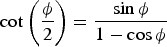 $\cot \left( {\displaystyle{\phi \over 2}} \right) = \displaystyle{{\sin \phi} \over {1 - \cos \phi}} $
, we have
 $${\dot {\bi \phi}} = \left[ {{\bi I} + \displaystyle{1 \over 2}\left\lceil {\bi \phi} \right\rceil + \displaystyle{1 \over {\phi ^2}} \left( {1 - \displaystyle{{\phi \sin \phi} \over {2\left( {1 - \cos \phi} \right)}}} \right)\left\lceil {\bi \phi} \right\rceil ^2} \right]{\bi \omega} _{NO}^O $$
This is the same as the differential equation of rotation vector.
Equations (16) and (18) were developed by Bortz (Reference Bortz1971) in a lengthy geometry method, and later simplified by several other researchers (Nazaroff, Reference Nazaroff1979; Jiang, Reference Jiang1991). The Bortz equations achieved the exact expression of non-commutativity and show how previous rotations interact with the current angular velocity to obtain one final rotation. When using the Lie group method, the angular velocity can be regarded as the Lie algebra of the so (3) group, thus the Baker-Campbell-Hausdorff theorem can be applied to describe how finite rotations can combine into one single rotation. The rotation vector obtained by Bortz is exactly the bch of angular velocity in Lie group theory, and can be computed according to Equation (6).
In the above, we show how Lemma 1 can be used to obtain the same outcome as Bortz's work in a simpler mathematical way. The following part also extends in the same way to obtain solutions on other manifolds used in INS algorithms.
2.3. Differential Equations On se (3)
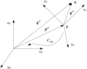
For a point q ∈ R 3 in frame O, its position vector in the reference frame N can be expressed as
 $${\bi q}^N = {\bi p}^N + {\bi C}_{NO}^{} {\bi q}^O $$
where p N is the coordinates of the origin of frame O relative to frame N, the superscripts is the corresponding measured frame. See Figure 1.
General motion of frame O respect to frame N.

The transformation can form a special Euclidean group se (3), as a 4 × 4 matrix of the form
 $${\bi Y}_{NO}^{} = \left[ {\matrix{ {{\bi C}_{NO}^{}} & {{\bi p}^N} \cr 0 & 1 \cr}} \right] \in {\smallcaps SE}\left( 3 \right)$$
se (3) is also a subgroup of a matrix Lie group, with the unit determinant as the group property. The differential equation can be given as
 $$\eqalign{& \left[ {\matrix{ {{\dot {\bi C}}_{NO}^{}} & {{\dot {\bi p}}^N} \cr 0 & 0 \cr}} \right] = \left[ {\matrix{ {{\bi C}_{NO}^{}} & {{\bi p}^N} \cr 0 & 1 \cr}} \right]\left[ {\matrix{ {\left\lceil {{\bi \omega} _{NO}^O} \right\rceil} & {{\bi v}_N^O} \cr 0 & 0 \cr}} \right] \cr & \quad \Leftrightarrow {\dot {\bi Y}}_{NO} = {\bi Y}_{NO} \left\lceil {{\bi V}_{NO}^O} \right\rceil}$$
where
 $\left\lceil {{\bi V}_{NO}} \right\rceil $
is the matrix representation of the vector
 ${\bi V}_{NO} = ({\bi v}_N^O ;{\bi \omega} _{NO}^O ) \in {\bf {\opf R}}^6 $
, and
 ${\bi v}_N^O $
is the velocity with respect to frame N coordinated in frame O. By comparing to Equation (1), we can see
 $\left\lceil {{\bi V}_{NO}} \right\rceil $
belongs to the Lie algebraFootnote
2
of
se
(3), denoted by
 ${\rm {\frak s}{\frak e}}(3)$
. Just as the Lie bracket of
 ${\rm {\frak s}{\frak o}}(3)$
, the Lie bracket on
 ${\rm {\frak s}{\frak e}}(3)$
is also the matrix commutator given as
 $$\left[ {\left\lceil {{\bi V}_1} \right\rceil, \left\lceil {{\bi V}_2} \right\rceil} \right] = \left\lceil {{\bi V}_1} \right\rceil \left\lceil {{\bi V}_2} \right\rceil - \left\lceil {{\bi V}_2} \right\rceil \left\lceil {{\bi V}_1} \right\rceil $$
Making use of the adjoint operator defined by
 $$ad_{\bi V} = \left[ {\matrix{ {\left\lceil {\bi \omega} \right\rceil} & {\left\lceil {\bi v} \right\rceil} \cr 0 & {\left\lceil {\bi \omega} \right\rceil} \cr}} \right]$$
The Lie bracket is readily obtained as
 $\left[ {\left\lceil {{\bi V}_1} \right\rceil, \left\lceil {{\bi V}_2} \right\rceil} \right] = \left\lceil {ad_{V1} {\bi V}_2} \right\rceil $
Following Lemma 1, the solution to Equation (21) is the exponential of some Lie algebra
 ${\bi \varphi } \in {\rm {\frak s}{\frak e}}\left( 3 \right)$
, given as
 $${\bi Y}\left( t \right) = {\bi Y}\left( 0 \right)\exp ({\bi \varphi} )$$
where
 ${\bi \varphi } \in {\rm {\frak s}{\frak e}}\left( 3 \right)$
satisfies the differential equation
 $${\dot {\bi \varphi}} \left( t \right) = d\exp _{ - {\bi \varphi}} ^{ - 1} {\bi V}_{NO}^O $$
Similar to the exponential map on
 ${\rm {\frak s}{\frak o}}\left( 3 \right)$
, the exponential of
 ${\bi \varphi } \in {\rm {\frak s}{\frak e}}\left( 3 \right)$
is originally given as
 $$\exp \left( {\bi \varphi} \right) = \exp m(\left\lceil {\bi \varphi} \right\rceil ) = \sum\limits_{\,j = 0}^\infty {\displaystyle{{\left\lceil {\bi \varphi} \right\rceil} \over {\,j!}}^j} $$
By using Rodrigues’ formula, the close form of the exponential map of
 ${\bi \varphi } = \left( {{\bi \lambda };\!{\bi \phi }} \right) \in {\rm {\frak s}{\frak e}}\left( 3 \right)$
is (Jonghoon and Chung, Reference Jonghoon and Chung2005), for
φ
= 0
 $$\exp ({\bi \varphi }) = \left[ {\matrix{ {\bi I} & {\bi \lambda } \cr 0 & 1 \cr } } \right]$$
for nonzero φ
 $$\exp ({\bi \varphi }) = \left[ {\matrix{ {\bf \Omega } & {\displaystyle{1 \over {\phi ^2}}\left( {\left( {{\bi I} - \Omega } \right)\left( {{\bi \phi } \times {\bi \lambda }} \right) + {\bi \phi {\phi }^{\prime}\lambda }} \right)} \cr 0 & 1 \cr } } \right]$$
where
 ${\bf \Omega} = \exp ({\bi \phi} ) = \exp m(\left\lceil {\bi \phi} \right\rceil ) \in {\smallcaps SO}(3)$
 $d\exp _{{\bi - \varphi}} ^{ - 1} $
can be computed by Equation (7), however, we will introduce the close form of it for efficient computation, before this, we firstly define some parameters, they are
 $$s = \displaystyle{{\sin \displaystyle{\phi \over 2}} \over {\displaystyle{\phi \over 2}}}\quad\quad\quad c = \cos \left( {\displaystyle{\phi \over 2}} \right)$$
They are used to compute
 $$\beta = s^2 \quad {\rm and} \quad \gamma = \displaystyle{c \over s}$$
For Lie algebra
 ${\bi \varphi } = \left( {{\bi \lambda };\!{\bi \phi }} \right) \in {\rm {\frak s}{\frak e}}\left( 3 \right)$
with nonzero
φ
, the inverse of the differential of the exponential map are presented as a 6 × 6 matrix
 $$d\exp _{{\bf -} {\bi \varphi}} ^{ - 1} = \left[ {\matrix{ {d\exp _{{\bf -} {\bi \phi}} ^{ - 1}} & {{\bi D} + \displaystyle{1 \over 2}\left\lceil {\bi \lambda} \right\rceil} \cr 0 & {d\exp _{{\bf -} {\bi \phi}} ^{ - 1}} \cr}} \right]$$
where
 $${\bi D} = \displaystyle{{1 - \gamma} \over {\left \Vert \phi \right \Vert ^2}} \left\lceil {{\bi \lambda}, {\bi \phi}} \right\rceil + \displaystyle{{\displaystyle{1 \over \beta} + \gamma - 2} \over {\left \Vert \phi \right \Vert ^4}} ({\bi \phi ^{\prime}\lambda} )\left\lceil {\bi \phi} \right\rceil ^2 $$
φ
′ is the transpose of
φ
, and
 $\left\lceil {{\bi \lambda}, {\bi \phi}} \right\rceil = \left\lceil {\bi \lambda} \right\rceil \left\lceil {\bi \phi} \right\rceil + \left\lceil {\bi \phi} \right\rceil \left\lceil {\bi \lambda} \right\rceil $
If φ = 0, then D = 0. When sin (φ/2) = 0 and φ ≠ 0, the close-form becomes singular, at this time Equation (7) can be used to approximate it.
From the last section, we have seen that Lie algebra φ is indeed the rotation vector given by Bortz. Here we will investigate the translation part in ϕ , that is λ . As presented in Equation (20), the vector in the last column represents the position vector of exp( ϕ ) with respect to Y (0), denoted by Δ r
 $$\Delta {\bi r} = \displaystyle{1 \over {\phi ^2}}\left( {\left( {{\bi I} - \Omega } \right)\left\lceil {\bi \phi } \right\rceil {\bi \lambda } + {\bi \phi {\phi }^{\prime}\lambda }} \right)$$
Take the same function of φ defined in Savage, (Reference Savage2006b) as
 $$f_1 \left( \phi \right) = \displaystyle{{\sin \phi} \over \phi} \quad\quad f_2 \left( \phi \right) = \displaystyle{{1 - \cos \phi} \over {\phi ^2}} \quad {\rm and}\quad f_3 \left( \phi \right) = \displaystyle{{1 - f_1 \left( \phi \right)} \over {\phi ^2}} $$
Then take Equation (16) into Equation (31)
 $$\Delta {\bi r} = \displaystyle{1 \over {\phi ^2}} \left[ {\left( {I - I - f_1 (\phi )\left\lceil {\bi \phi} \right\rceil - f_2 (\phi )\left\lceil {\bi \phi} \right\rceil ^2} \right)\left\lceil {\bi \phi} \right\rceil + {\bi \phi \phi ^{\prime}}} \right]{\bi \lambda} $$
Note that
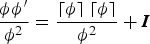 $\displaystyle{{{\bi \phi \phi '}} \over {\phi ^2}} = \displaystyle{{\left\lceil {\bi \phi} \right\rceil \left\lceil {\bi \phi} \right\rceil} \over {\phi ^2}} + {\bi I}$
and
 $\left\lceil {\bi \phi} \right\rceil ^3 = - \phi ^2 \left\lceil {\bi \phi} \right\rceil $
, the translation can be given as
 $$\Delta {\bi r} = \left[ {{\bi I} + f_2 (\phi )\left\lceil {\bi \phi} \right\rceil + f_3 (\phi )\left\lceil {\bi \phi} \right\rceil ^2} \right]{\bi \lambda} $$
Comparing to the translation part in DQ (Wu, Reference Wu2006), λ is indeed the same as the dual part of the screw vector.
The differential equation of λ is
 $${\dot {\bi \lambda}} = \left( {{\bi D} + \displaystyle{1 \over 2}{\bi \lambda}} \right){\bi \omega} _{NO}^O + d\exp _{ - {\bi \phi}} ^{ - 1} {\bi v}_N^O $$
In fact, the above equation is also the same as the differential equation of the dual part in DQ (See Appendix A for details). As the real part of DQ is also the same as Bortz’ rotation vector, the se (3) group and DQ are analytically the same.
Several papers have discussed the differences of the translations in DQ and Savage's translations vectors (Wu, Reference Wu2006; Wu and Xiao, Reference Wu and Xiao2011; Savage, Reference Savage2006a). As λ is equivalent to the translation part of DQ, the comparisons of λ and translation vectors are similar to these works. In brief, λ is the same as a velocity transition vector, however, λ can hardly deduce a PTV that can reduce to a double integral of specific force acceleration when angular-rate/specific-forces are constant.
2.4. Other Lie Groups Used In INS
Applications of the general Lie group method in two useful matrix Lie group so (3) and se (3) are presented. However, as we can see, this general method is not constrained to a matrix Lie group. Any Lie group differential equation satisfying Equation (1) can be solved in this way. In fact, quaternion and dual quaternion are also subgroups of Lie group, with the unit norm as their group identity and quaternion/dual quaternion product as the group operator. Their differential equations areFootnote 3
 $${\dot {\bi q}} = {\bi q}\left( {\displaystyle{1 \over 2}{\bi \omega }_{NO}^O } \right) \quad {\rm and} \quad {\mathop{\bi q}\limits^{\dot\frown}} = {\mathop{\bi q}\limits^{\frown}}\left( {\displaystyle{1 \over 2} {\mathop{\bi w}\limits^{\frown}}_{NO}^O } \right)\,$$
where
q
is quaternion,
 ${\mathop{\bi q}\limits^{\frown}}$
is dual quaternion and
 ${\mathop{\bi w}\limits^{\frown}}_{NO}^O$
is the corresponding dual vector.
These differential equations are in exactly the same form as Equation (1). Furthermore, the dual/angular vector product also satisfies the Lie bracket property. Thus, the general Lie group method can also apply to quaternion and dual quaternion (see Appendix B).
The existing solutions of DCM and dual quaternion are re-derived by using the Lie group method, we also introduced the se (3) group for rigid body dynamics. Traditionally, the maps between kinematic vectors and quaternion/ dual quaternion/ DCM are given by analysing the geometry relationships between them which involve a number of algebraic manipulations. However, this can be greatly simplified when taking a modern treatment of the differential equations as they are Lie group equations. Thus, the map between kinematic vectors and quaternion/ dual quaternion/ DCM/ se (3) is indeed the exponential map. The differential of the kinematic vector can be given by a single step by using a general differential of the exponential map.
3. STRAPDOWN INERTIAL NAVIGATION ALGORITHMS BASED ON se (3).
3.1. Navigation Differential Equations
The general Lie group method and its applications in rigid body dynamics are introduced in the last section. In this section, we will design an INS algorithm based on this unified Lie group method in se (3) form. This new algorithm acts as an example of a Lie group-based INS algorithm, and as a comparison with the previous DQ algorithm which is designed in a primitive geometrical way.
Before introducing the new algorithm, we define three coordinate frames, they are body frame B, Earth frame E and inertial frame I. Frame B is aligned with the strapdown inertial sensors axis. Frame E has its origin at centre of Earth, and one axis parallel to Earth's polar axis, the other axis fixed to the Earth and parallel to the equatorial plane. Inertial frame I is defined as the Earth frame at time instant t = 0.
As we know, the velocity update algorithm in the INS system is a process of integrating the total acceleration. The total acceleration is the sum of gravitational acceleration and the specific force acceleration, in the inertial frame it can be expressed as
 $${\ddot {\bi r}}^I = {\bi g}^I + {\bi s}^I $$
where r is the position vector of the body frame, g is the gravitational acceleration, s is the specific force acceleration. Superscripts mean they are coordinated in frame I.
Velocity and position are the integrations of Equation (36), they are given as
 $$\displaylines{{\dot {\bi r}}^I = {\dot {\bi r}}^I \left( 0 \right) + \int_0^t {\left( {{\bi g}^I + {\bi s}^I} \right)d\tau} \cr {\bi r}^I = {\bi r}^I \left( 0 \right) + {\dot {\bi r}}^I \left( 0 \right)t + \int_0^t {\left[ {\int_0^{\tau _1} {\left( {{\bi g}^I + {\bi s}^I} \right)d\tau _2}} \right]d\tau _1}.} $$
In a typical strapdown INS, the specific force acceleration is measured in the body frame, and the gravitational acceleration is calculated in the Earth frame or the local frame. To avoid unnecessary coordinate transformation, it is more convenient to treat the gravitational acceleration and the specific force acceleration separately.
Define the thrust velocity
 ${\bi v}_t^{} $
as the integration of the specific force acceleration, i.e.
 $${\bi v}_t^I = \,\int_0^t {{\bi s}^I d\tau}. $$
Similarly, define the gravitational velocity
 ${\bi v}_g^{} $
as the sum of initial velocity and integration of gravitational acceleration, i.e.
 $${\bi v}_g^I = {\dot {\bi r}}^I \left( 0 \right) + \int_0^t {{\bi g}^I d\tau}. $$
Thus, the velocity can be written as
 ${\dot {\bi r}}^I = {\bi v}_t^I + {\bi v}_g^I $
. Since the velocity of the vehicle can be decomposed into the thrust velocity
v
t
and gravitational velocity
v
g
, one can calculate them in two independent frames parallel to the body frame and the Earth frame. To do this, the velocity frames T and G are introduced (Wu et al., Reference Wu, Hu, Hu, Li and Lian2005).
For thrust velocity frame T, its axes are aligned with those of body frame B, vector from Earth's centre to its origin is exactly thrust velocity. For gravitational velocity frame G, its axes are aligned with Earth frame E, the vector from Earth's centre to its origin is exactly gravitational velocity.
Firstly, consider the inertial frame I and the thrust velocity frame T. Note that, it is the thrust velocity that represents the position vector of frame T, as a consequence, the derivative of the translation is not the velocity but the specific acceleration.
Suppose a group element
Y
IT
∈
se
(3) characterises the general displacement of frame T. Since frame T is parallel to the body frame, we have
 ${\bi \omega} _{IT}^T = {\bi \omega} _{IB}^B $
and
 ${\bi C}_{IT}^{} = {\bi C}_{IB}^{} $
. Then, the Lie algebra of
Y
IT
∈
se
(3) can be written as
 ${\bf \Lambda} _{IT}^T = ({\bi s}_{}^T ;{\bi \omega} _{IT}^T ) = ({\bi s}_{}^B ;{\bi \omega} _{IB}^B ) \in {\rm {\frak s}{\frak e}}(3)$
.
The rate equation of Y IT can be acquired by using Equation (21), as the form
 $$\eqalign{& \left[ {\matrix{ {{\dot {\bi C}}_{IT}^{}} & {{\dot {\bi v}}_t^I} \cr 0 & 0 \cr}} \right] = \left[ {\matrix{ {{\bi C}_{IT}^{}} & {{\bi v}_t^I} \cr 0 & 1 \cr}} \right]\left[ {\matrix{ {\left\lceil {{\bi \omega} _{IT}^T} \right\rceil} & {{\bi s}^T} \cr 0 & 0 \cr}} \right] \cr & \qquad \qquad {\dot {\bi Y}}_{IT} = {\bi Y}_{IT} \left\lceil {{\bf \Lambda} _{IT}^T} \right\rceil}$$
The direction cosine matrix
 ${\bi C}_{IT}^{} $
and thrust velocity
 ${\bi v}_t^I $
can be derived from the solution of the above equation.
Secondly, consider the inertial frame I and the gravitational velocity frame G. Note that it is the gravitational velocity that represents the position vector of frame G, so the derivative of the translation is not the velocity but the gravitational acceleration.
Let
Y
IG
∈
se
(3) describe the general displacement of frame G, the Lie algebra of
Y
IG
∈
se
(3) can be expressed as
 ${\bf \Lambda} _{IG}^G = ({\bi g}_{}^G ;{\bi \omega} _{IG}^G ) = ({\bi g}_{}^E ;{\bi \omega} _{IE}^E ) \in {\rm {\frak s}{\frak e}}(3)$
. The differential equation is
 $$\eqalign{& \left[ {\matrix{ {{\dot {\bi C}}_{IG}^{}} & {{\dot {\bi v}}_g^I} \cr 0 & 0 \cr}} \right] = \left[ {\matrix{ {{\bi C}_{IG}^{}} & {{\bi v}_g^I} \cr 0 & 1 \cr}} \right]\left[ {\matrix{ {\left\lceil {{\bi \omega} _{IG}^G} \right\rceil} & {{\bi g}^G} \cr 0 & 0 \cr}} \right] \cr & \qquad \qquad {\dot {\bi Y}}_{IG} = {\bi Y}_{IG} \left\lceil {{\bf \Lambda} _{IG}^G} \right\rceil}$$
The direction cosine matrix
 ${\bi C}_{IG}^{} $
and gravitational velocity
 ${\bi v}_g^I $
can be derived from the solution of the above equation.
To obtain position, we define a position frame U, with its axes aligned with those of the Earth frame; the vector from Earth's centre to its origin is exactly the position vector of the vehicle. By definition, we have
 ${\bi \omega} _{IU}^U = {\bi \omega} _{IE}^E $
and
 ${\bi v}_I^U = {\bi C}_{UI}^{} {\bi v}_I^I = {\bi C}_{EI}^{} ({\bi v}_t^I + {\bi v}_g^I )$
. Suppose a group element
Y
IU
∈
se
(3) shows the displacement of frame U, and the corresponding Lie algebra is
 ${\bi V}_{IU}^U = ({\bi v}_I^U ;{\bi \omega} _{IU}^U ) \in {\rm {\frak s}{\frak e}}(3)$
.
The rate equation of Y IU is
 $$\eqalign{& \left[ {\matrix{ {{\dot {\bi C}}_{IU}^{}} & {{\dot {\bi r}}^I} \cr 0 & 0 \cr}} \right] = \left[ {\matrix{ {{\bi C}_{IU}^{}} & {{\bi r}^I} \cr 0 & 1 \cr}} \right]\left[ {\matrix{ {\left\lceil {{\bi \omega} _{IU}^U} \right\rceil} & {{\bi v}_I^U} \cr 0 & 0 \cr}} \right] \cr & \qquad \qquad {\dot {\bi Y}}_{IU} = {\bi Y}_{IU} \left\lceil {{\bi V}_{IU}^U} \right\rceil}$$
By solving the above equation, the position vector r I can be obtained.
So far, the navigation equations are presented in the form of
se
(3) and
 ${\rm {\frak s}{\frak e}}(3)$
. The navigation parameters (attitude, velocity and position) in frame I can be acquired by solving Equations (39), (40) and (41) and they can be expressed in any other navigation frames, i.e., the parameters in Earth frame are
 $$\eqalign{& {\bi C}_{EB} = {\bi C}_{EI}{\bi C}_{IB} = \left( {{\bi C}_{IG}} \right)^{\prime}{\bi C}_{IT} \cr & {\bi v}_E^E = {\bi v}_I^E - {\bi \omega }_{IE}^E \times {\bi r}^E = {\bi v}_t^E + {\bi v}_g^E - {\bi \omega }_{IE}^E \times {\bi r}^E \cr & {\bi r}^E = {\bi C}_I^E {\bi r}^I = \left( {{\bi C}_G^I } \right)^{\prime}{\bi r}^I} $$
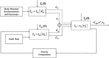
The fundamental mechanism of the strapdown INS algorithm based on
se
(3) and
 ${\rm {\frak s}{\frak e}}\left( 3 \right)$
is presented in Figure 2. The navigation frame is chosen as the Earth frame.
The fundamental mechanism of the strapdown INS algorithm based on Lie group and Lie algebra.

3.2. Numerical Integration Algorithms
Though various numerical integration methods have been developed to solve Lie group differential equations, the integration method in INS is, somehow, different. The existing methods impose a Runge-Kutta-like method on manifolds (Iserles et al., Reference Iserles, Munthe-Kass, Norsett and Zanna2000). However, in INS we need to develop numerical algorithms to achieve minimal errors under coning/sculling environments. In this section, a new update algorithm is developed to integrate the se (3) group rate equations. The new algorithm is structured similar to the traditional two-speed approach (Ignagni, Reference Ignagni2003).
Note that all the rate Equations (39), (40) and (41) have the same form as
 $${\dot {\bi Y}} = {\bi Y}\left\lceil {\bf \Lambda} \right\rceil \quad {\rm or}\quad {\dot {\bi Y}} = {\bi Y}\left\lceil {\bi V} \right\rceil $$
where superscripts and subscripts are neglected for brevity.
We will take the differential equation of the velocity frame as the general form for further discussion. The Lie algebra Λ is generally expressed as
 ${\bf \Lambda } = ({\bi a};{\bi \omega }) \in {\rm {\frak s}{\frak e}}(3)$
in this section. As shown in Equation (24), the solution of the differential equation is the exponential of a Lie algebra and suppose it is expressed as
 ${\bi \Phi } = \left( {{\bi \eta };{\bi \phi }} \right) \in {\rm {\frak s}{\frak e}}\left( 3 \right)$
.
The differential equation of the Lie algebra
 ${\bi \Phi } = \left( {{\bi \eta };{\bi \phi }} \right) \in {\rm {\frak s}{\frak e}}\left( 3 \right)$
is
 $${\dot {\bi \Phi}} \left( t \right) = d\exp _{ - {\bi \Phi}} ^{ - 1} {\bf \Lambda} $$
Taking
 $d\exp _{ - {\bf \Phi}} ^{ - 1} $
into Equation (42), and adopting a second-order accuracy, that is adopting the first two terms in Equation (7) , we haveFootnote
4
 $${\dot {\bi \Phi}} = {\bf \Lambda} + \displaystyle{1 \over 2}[{\bi \Phi}, {\bf \Lambda} ]$$
Let
 ${\bi \Phi } \in {\rm {\frak s}{\frak e}}\left( 3 \right)$
be small enough, Equation (43) can be approximated by
 $${\dot {\bi \Phi}} = {\bf \Lambda} + \displaystyle{1 \over 2}[{\bi \alpha}, {\bf \Lambda} ] \quad {\rm where} \quad {\bi \alpha} = \,\int_{t_k} ^t {\bf \Lambda} dt$$
Integrating Equation (44) during a minor interval, the Lie algebra Δ Φ is
 $$\Delta {\bi \Phi} = {\hat {\bi \alpha}} + \displaystyle{1 \over 2}\int_{t_k} ^{t_{k + 1}} {[{\hat {\bi \alpha}}, {\bf \Lambda} ]} dt$$
where
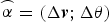 ${\mathop{\bi \alpha}\limits^{\frown}} = \left( {\Delta {\bi v};\Delta {\bi \theta}} \right)$
is the accumulated incremental of Lie algebra Λ during the current minor interval. Using Δ
Φ
s
= (Δ
η
s
; Δ
φ
s
) to denote the integrating term, we can investigate the components separately. The integration term in Equation (45) is equivalent to the following formulae
 $$\Delta {\bi \phi} _s = \displaystyle{1 \over 2}\int_{t_k} ^{t_{k + 1}} {\left[ {\Delta {\bi \theta} \times {\bi \omega}} \right]} dt \quad {\rm and} \quad \Delta {\bi \eta} _s = \displaystyle{1 \over 2}\int_{t_k} ^{t_{k + 1}} {\left[ {\Delta {\bi \theta} \times {\bi a} + \Delta {\bi v} \times {\bi \omega}} \right]} dt$$
Δ φ s and Δ η s are exactly the same as the coning and the sculling in the conventional algorithm (Savage, Reference Savage1998a; Savage, Reference Savage1998b). As Δ Φ s combined the two terms as a whole, it is named as a screw correction.
Similar to the calculation of coning and sculling, the general screw correction can be approximated by the sum of all possible Lie brackets formed from N sub-minor sensor-data intervals, making up a minor computational interval. An approximation can be formulated as
 $$\Delta {\bi \Phi} _s = \sum\limits_{i = 1}^N {\sum\limits_{\,j \gt i}^N {K_{ij}}}\left[{\mathop{\bi \alpha}\limits^{\frown}}_i, {\mathop{\bi \alpha}\limits^{\frown}}_j \right] $$
where
 ${\mathop{\bi \alpha}\limits^{\frown}}_i $
is the incremental Lie algebra over the i
th
sub-minor interval; The optimal coefficients K
ij
are exactly the same as those in conventional algorithm (Ignagni, Reference Ignagni2003). For example when N = 2, the coefficient K
12 = 2/3.
After the screw vector Φ is calculated, the numerical solution to the group rate equation can be given as
 $${\bi Y}(t + \Delta T) = {\bi Y}(t)\exp ({\bi \Phi} (\Delta T))$$
where Y (t) is the previous Lie group and Y (t + ΔT) is the current one, exp( Φ (ΔT)) is the updating Lie group during the major interval.
Since the exponential map contains trigonometric functions which are very hard to compute in real time, approximated truncation of trigonometric series are adopted to simplify it. For example, a fourth-order approximation is given as
 $$\sin (\phi ) = \phi + \displaystyle{{\phi ^3} \over {3!}} \quad \cos (\phi ) = 1 - \displaystyle{{\phi ^2} \over {2!}} + \displaystyle{{\phi ^4} \over {4!}}$$
This approximation is equivalent to adopting the corresponding terms in the series formula given in Section 2.
4. SIMULATIONS
In Section 2 we demonstrated that se (3) group is analytically equivalent to dual quaternion. In this section we will show that the new se (3) based INS algorithm achieves the same accuracy as DQ numerically. A variety of numerical simulations were conducted by using Matlab2010. The local-level frame is defined with x directing north and y directing upward vertically. In the simulations, we use an ideal trace generator which feeds on two inputs: the local frame acceleration and the Euler angle rate, to produce gyro/accelerometer outputs as well as the vehicle's ideal navigation parameters, namely, attitude angles, velocity vector and position. Algorithm errors are computed according to these ideal navigation parameters.
The inputs of the trace generator are configured as 20 sin(2π ft)(m/s2) for every channel of ground acceleration and 2πf cos(2πft)(rad/s) for every channel of Euler angle rate. The sampling frequency of gyro/accelerometer is 100Hz. At the beginning, the vehicle stands still on the ground of the Earth at latitude 30°, longitude 110° and altitude 0 m, and the Euler angles are 0°. Gravitation is calculated in the local-level frame and then transformed to the Earth frame for the sake of consistency (Chatfield, Reference Chatfield2013; Wei and Schwarz, Reference Wei and Schwarz1990). The two-sample algorithm is adopted and a fourth-order truncation of trigonometric series is used in the simulations. The DQ algorithm is conducted by Simulink modules and the new se (3) algorithm is conducted by m-files. In order to make comparisons, the simulation results are transformed from the Earth frame to the local level frame, the transformation algorithm is based on Wu et al. (Reference Wu, Wang and Hu2003). The simulations are conducted under ideal conditions.
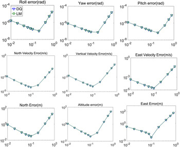
Firstly, the input frequency is set to cover a list of discrete frequencies from 0·01 to 1Hz, i.e. f = 0·01, 0·02, 0·04, 0·06, 0·08, 0·1, 0·2, 0·4, 0·6, 0·8Hz. The runtime is set to be 1800 seconds. The Maximum Absolute Errors (MAE) are shown in Figure 3 as functions of the input signal frequency. Simulations show that the se (3) algorithm is similar to the DQ algorithm in accuracy and turning frequency.
(With ideal inertial sensors) MAEs(log-log plot) in Euler angles/velocity/position as function of input signal frequency.

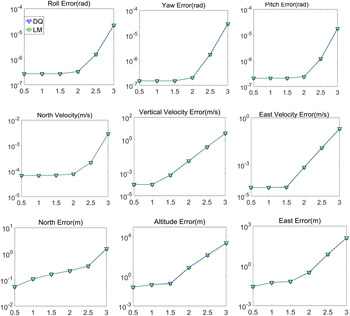
Simulations are also conducted to test the long range performance of the algorithms. The input signal frequency is set to 0·06Hz, runtime is set to 0·5 hour, 1 hour, 1·5 hours, 2 hours, 2·5 hours, and 3 hours respectively. Results are shown in Figure 4. Simulations show that after 2 hours of navigation, errors grow faster in time. This is mainly due to the accumulated errors of the INS. We also notice that velocity and position errors in the vertical channel are obviously larger than east and north errors. This is mainly due to the inherent instability of the vertical channel, not the effects of the form of equations and integration methods.
(With ideal inertial sensors) MAEs(log plot) in Euler angles/velocity/position as function of time.

Though the
se
(3) algorithm shows no improvement in accuracy, the general Lie group method used in the design process shows its brevity and uniformity. Also
se
(3) and
 ${\rm {\frak s}{\frak e}}\left( 3 \right)$
are much more direct than DQ, and also keep the mathematical prerequisites to minimum as they are usual matrix and vector operations. However, the new algorithm is not as efficient as the DQ algorithm in computation. But their gap in computation cost is not large, and modern computer technology enables the new algorithm to be viable for real time applications (see Appendix C for a detailed computation cost comparison).
5. CONCLUSIONS
This paper presents a unified method for INS algorithm design by using Lie group and Lie algebra. This method can be applied to Lie subgroups used in INS algorithms including the special orthogonal group so (3) and the special Euclidean group se (3), even quaternion and dual quaternion can be treated in this framework. By using this method, the solutions of the differential equations on these Lie subgroups can be easily obtained. Comparing to the previous lengthy geometrical methods, the Lie group method is a simpler unified one.
Based on this method, we developed a new INS algorithm by using
se
(3). The principle of inertial navigation is simplified as three group differential equations. We also formulated a new numerical integration algorithm to solve these group equations. Analytical and numerical comparisons show that the new algorithm achieves the same accuracy as the existing DQ algorithm. Though the
se
(3) algorithm has no improvement in accuracy, the general Lie group method used in the design process shows its brevity and uniformity. Also the vector and matrix representation of
se
(3) and
 ${\rm {\frak s}{\frak e}}\left( 3 \right)$
give us a more direct way to treat the rigid body motion than DQ. However, the computation cost of
se
(3) algorithm is a little bit larger than DQ, but modern computer technology enables the
se
(3) algorithm to be viable for real time applications.
ACKNOWLEDGMENTS
This work was supported by the National Natural Science Foundation of China (No.61503403, No.61573371). The authors would like to thank editors and anonymous reviewers for their insightful comments and constructive suggestions.
APPENDIX A. THE DIFFERENTIAL EQUATION OF λ
In Equation (34), we have
 $$\eqalign{& {\bi D} = \displaystyle{{1 - \gamma} \over {\left \Vert \phi \right \Vert ^2}} \left\lceil {{\bi \lambda}, {\bi \phi}} \right\rceil + \displaystyle{{\displaystyle{1 \over \beta} + \gamma - 2} \over {\left \Vert \phi \right \Vert ^4}} ({\bi \phi ^{\prime}\lambda} )\left\lceil {\bi \phi} \right\rceil ^2 \matrix{ {} & {\matrix{ {} & {} & {\matrix{ {} & {} & {} \cr}} & {} \cr}} \cr} \left\lceil {{\bi \lambda}, {\bi \phi}} \right\rceil = \left\lceil {\bi \lambda} \right\rceil \left\lceil {\bi \phi} \right\rceil + \left\lceil {\bi \phi} \right\rceil \left\lceil {\bi \lambda} \right\rceil \cr & \gamma = \displaystyle{{\phi \sin \phi} \over {2\left( {1 - \cos \phi} \right)}}\matrix{ {\matrix{ {\matrix{ {\matrix{ {\matrix{ {} & {} & {} \cr}} & {} \cr}} & {} \cr}} & {} \cr}} & {\matrix{ {} & {} & {} & {} \cr}} & {\matrix{ {} & {} & {} \cr}} \cr} \displaystyle{1 \over \beta} = \displaystyle{{\phi ^2} \over {2\left( {1 - \cos \phi} \right)}} \cr & d\exp _{ - {\bi \phi}} ^{ - 1} = {\bi I} + \displaystyle{1 \over 2}\left\lceil {\bi \phi} \right\rceil + \displaystyle{1 \over {\phi ^2}} \left( {1 - \displaystyle{{\phi \sin \phi} \over {2\left( {1 - \cos \phi} \right)}}} \right)\left\lceil {\bi \phi} \right\rceil ^2} $$
Taking the above equations into Equation (34), we have
 $$\eqalign{{\dot {\bi \lambda}} &= \left( {{\bi D} + \displaystyle{1 \over 2}{\bi \lambda}} \right){\bi \omega} _{NO}^O + d\exp _{ - {\bi \phi}} ^{ - 1} {\bi v}_N^O \cr & = {\bi v}_N^O + \displaystyle{1 \over 2}\left( {{\bi \phi} \times {\bi \lambda} + {\bi \lambda} \times {\bi \phi}} \right) + \displaystyle{1 \over {\phi ^2}} \left( {1 - \displaystyle{{\phi \sin \phi} \over {2\left( {1 - \cos \phi} \right)}}} \right) \left[{\bi \phi} \times \left( {\bi \phi} \times {\bi v}_N^O \right) \right. \cr & \quad \left. +\, {\bi \phi} \times \left( {{\bi \lambda} \times {\bi \omega} _{NO}^O} \right) + {\bi \lambda} \times \left({{\bi \phi} \times {\bi \omega}_{NO}^O}\right) \right] + \left[ {\displaystyle{{\phi + \sin \phi} \over {2\phi ^3 \left( {1 - \cos \phi} \right)}} - \displaystyle{2 \over {\phi ^4}}} \right]\left( {{\bi \phi ^{\prime}\lambda}} \right){\bi \phi} \times \left( {{\bi \phi} \times {\bi \omega}_{NO}^O}\right)}$$
This is exactly the same as the differential equation of the dual part in dual quaternion (Wu, Reference Wu2006).
APPENDIX B. APPLYING THE LIE GROUP METHOD TO DQ
By applying Lemma 1, the solution to the dual quaternion differential Equation (35) can be given as
 $${\hat {\bi q}}\left( t \right) = {\hat {\bi q}}\left( 0 \right)\exp \left( {\displaystyle{{{\hat {\bi \phi}}} \over 2}} \right)$$
where
 $$\exp \left( {\displaystyle{{{\hat {\bi \phi}}} \over 2}} \right) = \sum\limits_{\,j = 0}^\infty {\displaystyle{{\left( {\displaystyle{{{\hat {\bi \phi}} \times} \over 2}} \right)^n} \over {\,j!}}} $$
The differential equations of
 ${\hat {\bi \phi}} $
can be given by using Equation (7) as
 $${\dot {\hat {\bi \phi}}} = d\exp _{ - { \hat {\bi \phi}}} ^{ - 1} {\hat {\bi \omega}} = {\hat {\bi \omega}} + \displaystyle{1 \over 2}{\hat {\bi \phi}} \times {\hat {\bi \omega}} + \displaystyle{1 \over {12}}{\hat {\bi \phi}} \times \left( {{\hat {\bi \phi}} \times {\hat {\bi \omega}}} \right) +..... = \sum\limits_{\,j = 0}^\infty {\displaystyle{{B_j} \over {\,j!}}} \left( {{\hat {\bi \phi}} \times} \right)^j {\hat {\bi \omega}} $$
The resulting Equation (A1) and (A2) are exactly the same as Equations (43) and (35) in Wu et al. (Reference Wu, Hu, Hu, Li and Lian2005). Comparing the two approaches in deriving the solution to the dual quaternion differential equation, the Lie group method is a much simpler one.
APPENDIX C. COMPARISON OF se (3) AND DQ ALGORITHM IN COMPUTATION COST
To make the computation cost comparison more clear, we split the se (3) algorithm into the following equations.
 $${\bi Y}(t + \Delta T) = {\bi Y}(t)\exp ({\bi \Phi} (\Delta T))$$
where
 $$\exp ({\bi \Phi} (\Delta T)) = \left[ {\matrix{ {\Delta {\bi C}} & {\Delta {\bi v}} \cr {\bf 0} & 1 \cr}} \right]$$
 $$\Delta {\bi C} = \exp (\Delta {\bi \phi} ) = {\bi I} + \displaystyle{{\sin (\Delta \phi )} \over {\Delta \phi}} \left\lceil {\Delta {\bi \phi}} \right\rceil + \displaystyle{{1 - \cos \left( {\Delta \phi} \right)} \over {\phi ^2}} \left\lceil {\Delta {\bi \phi}} \right\rceil ^2 $$
 $$\Delta {\bi v} = \displaystyle{1 \over {\phi ^2}} \left( {\left( {{\bi I} - \Omega} \right)\left( {{\bi \phi} \times} \right) + {\bi \phi \phi ^{\prime}}} \right){\bi \eta} $$
As we can see, the se (3) group are expressed by usual matrices and vectors, one can develop numerical algorithms for computer implementation directly based on Equations (A3)–(A6).
Dual quaternion consists of the real part and the dual part, and they are computed separately in numerical integration algorithms by using the following equations.
 $$\eqalign{& {\bi q}\left( {t + \Delta T} \right) = {\bi q}\left( t \right) {\circ} {\bi q}\left( {\Delta T} \right) \cr & {\bi q^{\prime}}\left( {t + \Delta T} \right) = {\bi q}\left( t \right) \circ {\bi q^{\prime}}\left( {\Delta T} \right) + {\bi q^{\prime}}\left( t \right) \circ {\bi q}\left( {\Delta T} \right)} $$
where the real part q (ΔT) is
 $${\bi q}\left( {\Delta T} \right) = \cos \left( {\displaystyle{\sigma \over 2}} \right) + \displaystyle{{\bi \sigma} \over \sigma} \sin \left( {\displaystyle{\sigma \over 2}} \right)$$
And the dual part q ′(ΔT) is
 $${\bi q^{\prime}}\left( {\Delta T} \right) = - \displaystyle{{\sigma^{\prime}} \over 2}\sin \left( {\displaystyle{\sigma \over 2}} \right) + \displaystyle{{\sigma {\bi \sigma^{\prime}} - \sigma^{\prime}\!{\bi \sigma}} \over {\sigma^2}} \sin \left( {\displaystyle{\sigma \over 2}} \right) + \displaystyle{{\sigma^{\prime}\!{\bi \sigma}} \over {2\sigma}} \cos \left( {\displaystyle{\sigma \over 2}} \right)$$
The resulting Δ v is
 $$\Delta {\bi v} = 2{\bi q^{\prime}}\left( {\Delta T} \right) \circ {\bi q}^ {^\ast} \left( {\Delta T} \right)$$
As discussed earlier
φ
and
σ
are indeed the rotation vectors and calculated as
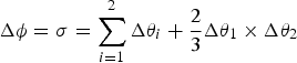 $\Delta {\bi \phi} = {\bi \sigma} = \sum\limits_{i = 1}^2 {\Delta {\bi \theta} _i} + \displaystyle{2 \over 3}\Delta {\bi \theta} _1 \times \Delta {\bi \theta} _2 $
, the translation vectors Δ
η
,
σ
′ are the same and calculated as
 $\Delta {\bi \eta} = {\bi \sigma '} = \displaystyle{2 \over 3}\left( {\Delta {\bi \theta} _1 \times \Delta {\bi v}_2 + \Delta {\bi v}_1 \times \Delta {\bi \theta} _2} \right)$
. We will only make computation cost comparisons of Equations (A3)–(A6) and Equations (A7)–(A10).
We evaluate the computation cost by the number of scalar additions, scalar multiplications, trigonometric functions and square root operations. For example, when given a vector ω = (ω 1; ω 2; ω 3), the norm is calculated as
 $$\omega = \sqrt {\omega _1 \omega _1 + \omega _2 \omega _2 + \omega _3 \omega _3} $$
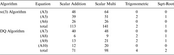
which requires three scalar multiplications, two scalar additions and one square root operation. In this manner, the computation cost of se (3) algorithm and DQ are given by Table A1.
Computation cost comparison of se (3) and DQ algorithm.

In the same computation sources, a single computation of se (3) algorithm takes 0·00023 seconds and DQ takes 0·00018 seconds.
Both the computation cost analysis and simulations show that DQ is more efficient than the se (3) algorithm, but their gap is not large. In fact, the difference between the two algorithms in computation cost stems from the different representation of the attitude part. In modern computer technology, most embedded systems are applicable to direction cosine matrix representation algorithms.