1 Introduction
The statistical characterisation of wall-pressure fluctuations under a turbulent boundary layer is necessary in many industrial applications. The wall-pressure fluctuations generated on the surface of air, land and maritime means of transport (where the curvature will typically generate adverse free-stream pressure gradients) are the cause of structural vibrations and noise that propagate inside the vehicle. Aircraft fuselage excitation due to pressure fluctuations is a significant source of cabin noise. Also, wall-pressure fluctuations can interfere with the signal of underwater sonar domes. More importantly for the purpose of this work, the pressure disturbances generated on the surface of wing profiles are scattered into acoustic waves at the trailing edge. This is a source of noise in low-speed fans and wind turbines. Moreover, it is the only remaining source of broadband noise for a subsonic fan operating in a homogeneous stationary flow. Due to the random nature of these disturbances, the generated noise is broadband and its intensity is directly proportional to that of the wall-pressure fluctuations, as expressed in analytical theories, among others Amiet (Reference Amiet1976) re-addressed by Roger & Moreau (Reference Roger and Moreau2005, Reference Roger and Moreau2012).
The experimental investigation of wall-pressure fluctuations dates back to the 50s (see the reviews of Bull (Reference Bull1996) and Cohen & Gloerfelt (Reference Cohen and Gloerfelt2018)) and still proves challenging nowadays. For instance, Salze et al. (Reference Salze, Bailly, Marsden, Jondeau and Juve2015) discussed the separation of the hydrodynamic and acoustic components of the spectrum of pressure fluctuations from the raw experimental data. In particular, the acoustic component has its energy peak at low wavenumbers for a given frequency and thus it is more likely to excite the structural modes of the underlying surface. It must also be remembered that the measured frequency–wavenumber spectrum is a convolution of the true spectrum of pressure fluctuations with the response function of the experimental apparatus. Prigent et al. (Reference Prigent, Engelman, Salze and Bailly2018) discussed the application of various numerical techniques for the deconvolution of the physical spectrum from the response function, although this remains an open problem. Another question that has been long debated is the choice of the relevant boundary-layer parameters for the scaling of measured wall-pressure spectra, which is the first step towards building empirical predictive models. This question has been treated in the works of Keith, Hurdis & Abraham (Reference Keith, Hurdis and Abraham1992) and Cipolla & Keith (Reference Cipolla and Keith2000).
Direct numerical simulation (DNS) of the turbulent boundary layer can provide plenty of information concerning the statistical properties of turbulence and of the wall-pressure fluctuations that it generates. Earlier attempts at DNS date back to the eighties with the work of Spalart & Leonard (Reference Spalart, Leonard, Durst, Launder, Lumley, Schmidt and Whitelaw1987), using a spectral method. Reynolds numbers representative of industrial applications have long been out of the reach of DNS codes until the advent of supercomputers, as seen in Borrell, Sillero & Jiménez (Reference Borrell, Sillero and Jiménez2013). However, DNS is still far from being considered a viable design tool. A compromise in terms of computational cost for the generation of broadband noise sources is the fast random particle mesh method, which superimposes a synthetic field of turbulent fluctuations to the mean flow calculated by a Reynolds-averaged Navier–Stokes (RANS) simulation (see Proskurov, Darbyshire & Karabasov Reference Proskurov, Darbyshire and Karabasov2017). However, this method depends on the assumed functional expression of the turbulence energy spectrum, as shown by Wohlbrandt et al. (Reference Wohlbrandt, Hu, Guérin and Ewert2016), similar to the family of methods that is presented in this paper.
The fastest way to estimate the wall-pressure power spectral density (PSD) for noise prediction is to use a model, either empirical or based on the analytical solution of the Poisson equation. Most empirical models are developed by selecting several databases of wall-pressure spectra in similar flow conditions and normalising them in order to highlight the dependence on some boundary-layer parameters. Then, a mathematical expression is developed to fit the collapsed curves. Corcos (Reference Corcos1964) made one of the first attempts to build a universal statistical model of the wall-pressure spectrum, which has been widely used to this day due to its simple mathematical formulation but is known to greatly overestimate the contribution to a given radian frequency of the wavenumber range below the convective ridge. Corrections to the low-frequency behaviour of Corcos’ model have been proposed, for instance, by Ffowcs Williams (Reference Ffowcs Williams1982) and Caiazzo, D’Amico & Desmet (Reference Caiazzo, D’Amico and Desmet2016). In the work of Schlinker & Amiet (Reference Schlinker and Amiet1981), the pressure PSD is normalised by the outer boundary-layer parameters, the displacement thickness
 $\unicode[STIX]{x1D6FF}^{\ast }$
and the external velocity
 $U_{e}$
, and plotted as a function of the corresponding reduced frequency
 $\tilde{\unicode[STIX]{x1D714}}=\unicode[STIX]{x1D714}\,\unicode[STIX]{x1D6FF}^{\ast }/U_{e}$
. This model is suitable for flat-plate, zero-gradient boundary layers, but it is not able to represent the quadratic rise with
 $\unicode[STIX]{x1D714}$
in the low-frequency range, predicted by Kraichnan (Reference Kraichnan1956b
) and Phillips (Reference Phillips1956), or the increase of the PSD magnitude under the effect of an adverse pressure gradient. The model of Chase (Reference Chase1980), expressed in terms of both outer and inner boundary-layer variables (with the introduction of the wall shear stress,
 $\unicode[STIX]{x1D70F}_{w}$
) represents a step forward because it accounts for the low-frequency rise. More recently, the model of Goody (Reference Goody2004), also expressed in terms of mixed inner and outer generalised variables, has included the effect of the Reynolds number on the extension of the overlap zone observed in the middle frequency range, where the normalised pressure PSD decreases approximately as
 $\unicode[STIX]{x1D714}^{-0.7}$
. Still, these models are calibrated on zero-pressure-gradient flow databases. The model of Rozenberg, Roger & Moreau (Reference Rozenberg, Roger and Moreau2008), on the contrary, preserves the main features of Goody’s but also takes into account the effect of the adverse pressure gradient, which can increase the wall-pressure spectrum of up to
 $10$
dB in the low-frequency range. Initially this model was formulated with reference to
 $\unicode[STIX]{x1D70F}_{w}$
, which can be difficult to estimate in some cases. However, its latest formulation published in Rozenberg, Robert & Moreau (Reference Rozenberg, Robert and Moreau2012) takes into account additional features of the boundary layer and substitutes the wall shear stress with the maximum shear stress in the flow. Catlett et al. (Reference Catlett, Anderson, Forest and Stewart2015) generalised Goody’s model in order to capture adverse-pressure-gradient effects as well. Hu’s model (Hu Reference Hu2018) aims at representing the wall-pressure frequency spectrum under arbitrary non-equilibrium flow conditions by using the shape factor
 $H=\unicode[STIX]{x1D6FF}^{\ast }/\unicode[STIX]{x1D703}$
for non-dimensionalisation, a parameter that is also representative of boundary-layer development history. The most recent and comprehensive comparison of all published empirical models is given by Lee (Reference Lee2018), who propose a formulation that is valid for a wide range of flow conditions.
The Poisson equation governing pressure fluctuations in a turbulent boundary layer can be used to build models that relate pressure and velocity statistics through relatively simple analytical formulations. Heisenberg (Reference Heisenberg1948) and Batchelor (Reference Batchelor1951) addressed the problem of pressure fluctuations in homogeneous and unbounded turbulence, developing equivalent formulations. Subsequently, Kraichnan (Reference Kraichnan1956a
) added an infinite plane boundary condition to the homogeneous turbulence problem and then included the effect of anisotropy of the length scales of turbulence as a first step towards the understanding of a real boundary layer. This theory was then extended to the case of non-homogeneity in the direction normal to the wall by Kraichnan (Reference Kraichnan1956b
) and Hodgson (Reference Hodgson1961). Whereas Kraichnan’s theory is formulated in the space domain, Hodgson adopted a wavenumber-domain approach. The results of these studies were essentially analytical and based on idealised flow models. Panton & Linebarger (Reference Panton and Linebarger1974) coupled the analytical wavenumber-domain solution of the Poisson equation with a realistic flow model, from which arose the necessity to develop a numerical integration method to compute the wall-pressure spectrum. Their approach was later taken up by Remmler et al. (Reference Remmler, Christophe, Anthoine and Moreau2010), who used a RANS flow solution to provide flow input data to the model. Peltier & Hambric (Reference Peltier and Hambric2007) and Slama, Leblond & Sagaut (Reference Slama, Leblond and Sagaut2018) coupled the space-domain solution of the Poisson equation with steady-state flow simulations. These different approaches will be discussed in the first part of this paper. Unlike the previous authors, Parchen (Reference Parchen1998) developed a prediction method based on an approximate solution of the Poisson equation, following the theory developed by Blake (Reference Blake1986), which gave rise to the so-called TNO-Blake family of models, (see Kamruzzaman et al.
Reference Kamruzzaman, Lutz, Würz, Shen, Zhu, Hansen, Bertagnolio and Madsen2012; Bertagnolio, Fischer & Zhu Reference Bertagnolio, Fischer and Zhu2014; Stalnov, Paruchuri & Joseph Reference Stalnov, Paruchuri and Joseph2016; Fischer, Bertagnolio & Madsen Reference Fischer, Bertagnolio and Madsen2017). The difference between the exact and the approximate solutions in terms of accuracy of the predicted spectrum will be discussed as well in this work. The purpose is to provide the most comprehensive analytical approach to the prediction of the wall-pressure PSD, unifying all other approaches in a common framework. In particular, it will be shown that the fundamental problem consists of the representation of the two-point statistics of the turbulent velocity across the boundary layer, taking into account inhomogeneity and anisotropy effects. The application case selected for this study is a controlled-diffusion aerofoil at a free-stream Mach number of
 $M=0.05$
and a chord-based Reynolds number of
 $Re_{c}=1.5\times 10^{5}$
, which presents an equilibrium turbulent boundary layer with an adverse pressure gradient on its suction side. This also represents an improvement, since most currently used models are calibrated on zero-pressure-gradient boundary layers (see Slama et al.
Reference Slama, Leblond and Sagaut2018). Turbulence and wall-pressure statistics are extracted from a state-of-the-art DNS in order to validate the different steps in the construction of the model. Flow and wall-pressure statistics extracted from the DNS are compared for validation with measurements performed in the anechoic wind tunnel of the Université de Sherbrooke.
The computation of wall-pressure spectra with formulations based on the Poisson equation may present difficulties from the numerical point of view due to the presence of multi-dimensional integrals. For this reason, the last section of this work presents a Monte Carlo integration technique which can tackle this problem efficiently and at a low computational cost.
2 Differential equation formulation
2.1 Poisson equation solution
The Poisson equation governing the pressure fluctuations in a turbulent boundary layer derives from the divergence of the incompressible momentum equation, introducing Reynolds decomposition into mean and fluctuating quantities, then subtracting the time-averaged equation. As a result, the Laplacian of pressure fluctuations is equal to the sum of two source terms,
 $$\begin{eqnarray}\frac{1}{\unicode[STIX]{x1D70C}}\unicode[STIX]{x1D6FB}^{2}\,p=\underbrace{-\,2\frac{\unicode[STIX]{x2202}u_{j}}{\unicode[STIX]{x2202}x_{i}}\frac{\unicode[STIX]{x2202}U_{i}}{\unicode[STIX]{x2202}x_{j}}}_{\mathit{turbulence-mean~shear}}\underbrace{-\,\frac{\unicode[STIX]{x2202}^{2}}{\unicode[STIX]{x2202}x_{i}\unicode[STIX]{x2202}x_{j}}(u_{i}u_{j}-\overline{u_{i}u_{j}})}_{\mathit{turbulence-turbulence}},\end{eqnarray}$$
where
 $i,j=1,2,3$
, with
 $1$
the streamwise,
 $2$
the wall-normal and
 $3$
the transverse direction. According to (2.1) the pressure fluctuation,
 $p$
, can be considered as generated by two separate mechanisms (see the review by Gerolymos, Sénéchal & Vallet (Reference Gerolymos, Sénéchal and Vallet2013)). One mechanism is the turbulence–mean shear interaction, expressing the fact that the corresponding pressure fluctuations react immediately to a change of the mean flow gradient and are linear with respect to velocity fluctuations. The other mechanism is the nonlinear interaction of different components of the velocity fluctuations, which is not immediately affected by a change in mean flow gradient. Equation (2.1) is solved with the Dirichlet boundary condition
 $$\begin{eqnarray}\lim _{x_{2}\rightarrow \infty }p=0,\end{eqnarray}$$
whereby the pressure fluctuation vanishes at an infinite distance from the wall and the overall pressure tends to its mean free-stream value, and the Neumann boundary condition
 $$\begin{eqnarray}\frac{\unicode[STIX]{x2202}p}{\unicode[STIX]{x2202}x_{2}}\bigg|_{x_{2}=0}=0\end{eqnarray}$$
following from the rigid wall assumption. The space-domain solution of (2.1) is expressed within a Green’s function approach as
 $$\begin{eqnarray}\frac{1}{\unicode[STIX]{x1D70C}}\,p(\boldsymbol{x},t)=\int _{\boldsymbol{x}^{\prime }}-\left[2\frac{\unicode[STIX]{x2202}}{\unicode[STIX]{x2202}x_{i}}\left(\frac{\unicode[STIX]{x2202}U_{i}}{\unicode[STIX]{x2202}x_{j}}\,u_{j}\right)\,G(\boldsymbol{x},\boldsymbol{x}^{\prime })+\frac{\unicode[STIX]{x2202}^{2}}{\unicode[STIX]{x2202}x_{i}\unicode[STIX]{x2202}x_{j}}(u_{i}u_{j}-\overline{u_{i}u_{j}})\,G(\boldsymbol{x},\boldsymbol{x}^{\prime })\right]\,\text{d}\boldsymbol{x}^{\prime },\end{eqnarray}$$
where the function
 $$\begin{eqnarray}G(\boldsymbol{x},\boldsymbol{x}^{\prime })=-\frac{1}{2\,\unicode[STIX]{x03C0}}\frac{1}{\Vert \boldsymbol{x}-\boldsymbol{x}^{\prime }\Vert }\end{eqnarray}$$
satisfies the boundary conditions for an impulse source. The partial derivatives applied to the velocity variables in (2.4) can be transferred to the Green’s function by repeated applications of integration by parts and of the divergence theorem, yielding the equivalent formulations
 $$\begin{eqnarray}\frac{1}{\unicode[STIX]{x1D70C}}\,p(\boldsymbol{x},t)=\int _{\boldsymbol{x}^{\prime }}-\left[2\left(\frac{\unicode[STIX]{x2202}U_{i}}{\unicode[STIX]{x2202}x_{j}}\,u_{j}\right)\,\frac{\unicode[STIX]{x2202}G(\boldsymbol{x},\boldsymbol{x}^{\prime })}{\unicode[STIX]{x2202}x_{i}}+\frac{\unicode[STIX]{x2202}}{\unicode[STIX]{x2202}x_{i}}(u_{i}u_{j}-\overline{u_{i}u_{j}})\,\frac{\unicode[STIX]{x2202}G(\boldsymbol{x},\boldsymbol{x}^{\prime })}{\unicode[STIX]{x2202}x_{j}}\right]\,\text{d}\boldsymbol{x}^{\prime }\end{eqnarray}$$
and
 $$\begin{eqnarray}\frac{1}{\unicode[STIX]{x1D70C}}\,p(\boldsymbol{x},t)=\int _{\boldsymbol{x}^{\prime }}-\left[2\left(\frac{\unicode[STIX]{x2202}U_{i}}{\unicode[STIX]{x2202}x_{j}}\,u_{j}\right)\,\frac{\unicode[STIX]{x2202}G(\boldsymbol{x},\boldsymbol{x}^{\prime })}{\unicode[STIX]{x2202}x_{i}}+(u_{i}u_{j}-\overline{u_{i}u_{j}})\,\frac{\unicode[STIX]{x2202}^{2}G(\boldsymbol{x},\boldsymbol{x}^{\prime })}{\unicode[STIX]{x2202}x_{i}\unicode[STIX]{x2202}x_{j}}\right]\,\text{d}\boldsymbol{x}^{\prime },\end{eqnarray}$$
where
 $$\begin{eqnarray}\frac{\unicode[STIX]{x2202}G(\boldsymbol{x},\boldsymbol{x}^{\prime })}{\unicode[STIX]{x2202}x_{i}}=\frac{1}{2\unicode[STIX]{x03C0}}\frac{\Vert x_{i}-x_{i}^{\prime }\Vert }{\Vert \boldsymbol{x}-\boldsymbol{x}^{\prime }\Vert ^{3}}\end{eqnarray}$$
and
 $$\begin{eqnarray}\frac{\unicode[STIX]{x2202}^{2}G(\boldsymbol{x},\boldsymbol{x}^{\prime })}{\unicode[STIX]{x2202}x_{i}\unicode[STIX]{x2202}x_{j}}=\frac{1}{2\unicode[STIX]{x03C0}}\left[\frac{\unicode[STIX]{x1D6FF}_{ij}}{\Vert \boldsymbol{x}-\boldsymbol{x}^{\prime }\Vert ^{3}}-3\frac{\Vert (x_{i}-x_{i}^{\prime })(x_{j}-x_{j}^{\prime })\Vert }{\Vert \boldsymbol{x}-\boldsymbol{x}^{\prime }\Vert ^{5}}\right].\end{eqnarray}$$
Equations (2.4), (2.6) and (2.7) are mathematically equivalent, so the choice is motivated by considerations of numerical stability of the integration algorithm. Peltier & Hambric (Reference Peltier and Hambric2007) and Slama et al. (Reference Slama, Leblond and Sagaut2018) selected equation (2.7). However, Hu, Reiche & Ewert (Reference Hu, Reiche and Ewert2017) argued that (2.6) provides the best numerical realisation of the turbulence–turbulence interaction contribution. In any case, the space-domain approach prescribes a three-dimensional integral for the computation of
 $p$
, whereby the cross-correlation of wall-pressure fluctuations corresponds to a six-dimensional integral, which must still be Fourier transformed numerically to obtain the wavenumber–frequency spectrum that is needed in acoustic predictions. Performing these numerical integrations with limited time and computational resources would inevitably lead to a loss of accuracy. For this reason, it is preferable to derive an analytical solution for the unsteady pressure directly in the wavenumber domain.
2.2 Modified Helmholtz equation
2.2.1 Turbulence–mean shear interaction term
In this section, the wavenumber-domain expression of the unsteady pressure at the wall is derived assuming that the only significant contribution is given by the turbulence–mean shear interaction component. This approach has its roots in the analytical considerations of Kraichnan (Reference Kraichnan1956a ) and Hodgson (Reference Hodgson1961). More recently, however, Slama et al. (Reference Slama, Leblond and Sagaut2018) argued that the two components have the same order of magnitude, based on the numerical integration of (2.7). The derivation of a wavenumber solution for the turbulence–turbulence interaction term is more cumbersome and requires a set of more restrictive hypotheses in order to get a simple closed-form formulation. For this reason, the turbulence–turbulence interaction component will be presented separately in § 2.4.
Assuming homogeneous turbulence in planes parallel to the wall, equation (2.1) can be Fourier transformed in space in the
 $(x_{1},x_{3})$
directions, yielding the following modified Helmholtz equation:
 $$\begin{eqnarray}\frac{\unicode[STIX]{x2202}^{2}\hat{p}(\boldsymbol{k},x_{2})}{\unicode[STIX]{x2202}x_{2}^{2}}-k^{2}\,\hat{p}(\boldsymbol{k},x_{2})=-2\,\unicode[STIX]{x1D70C}\,\text{i}\,k_{i}\,\frac{\unicode[STIX]{x2202}U_{i}}{\unicode[STIX]{x2202}x_{j}}\hat{u} _{j}(\boldsymbol{k},x_{2}),\end{eqnarray}$$
where the following convention for the Fourier transform is adopted:
 $$\begin{eqnarray}\displaystyle & \displaystyle \hat{p}(\boldsymbol{k},x_{2}) & \displaystyle =\frac{1}{4\unicode[STIX]{x03C0}^{2}}\iint _{-\infty }^{+\infty }p(\boldsymbol{x})\,\text{e}^{-\text{i}(k_{1}x_{1}+k_{3}x_{3})}\,\text{d}x_{1}\,\text{d}x_{3},\end{eqnarray}$$
 $$\begin{eqnarray}\displaystyle & \displaystyle \hat{Q}(\boldsymbol{k},x_{2}) & \displaystyle =\frac{1}{4\unicode[STIX]{x03C0}^{2}}\iint _{-\infty }^{+\infty }Q(\boldsymbol{x})\,\text{e}^{-\text{i}(k_{1}x_{1}+k_{3}x_{3})}\,\text{d}x_{1}\,\text{d}x_{3}.\end{eqnarray}$$
Furthermore, assuming that the only non-vanishing mean velocity gradient is that of the streamwise component,
 $U_{1}$
, in the wall-normal direction,
 $x_{2}$
, the source term is reduced to
 $$\begin{eqnarray}\frac{\unicode[STIX]{x2202}^{2}\hat{p}(\boldsymbol{k},x_{2})}{\unicode[STIX]{x2202}x_{2}^{2}}-k^{2}\,\hat{p}(\boldsymbol{k},x_{2})=-2\,\unicode[STIX]{x1D70C}\,\text{i}\,k_{1}\,\frac{\unicode[STIX]{x2202}U_{1}}{\unicode[STIX]{x2202}x_{2}}\hat{u} _{2}(\boldsymbol{k},x_{2}).\end{eqnarray}$$
It is demonstrated in appendix A that the wavenumber-domain solution for the pressure at the wall is
 $$\begin{eqnarray}\hat{p}(\boldsymbol{k},x_{2}=0)=2\,\text{i}\,\unicode[STIX]{x1D70C}\frac{k_{1}}{k}\int _{0}^{\infty }\frac{\unicode[STIX]{x2202}U_{1}(X_{2})}{\unicode[STIX]{x2202}x_{2}}\hat{u} _{2}(\boldsymbol{k},X_{2})\text{e}^{-k\,X_{2}}\,\text{d}X_{2}.\end{eqnarray}$$
The PSD of wall-pressure fluctuations is equal to the ensemble average of the product of (2.14) by its complex conjugate,
 $$\begin{eqnarray}\displaystyle \unicode[STIX]{x1D711}_{pp}^{TM}(\boldsymbol{k}) & = & \displaystyle 4\unicode[STIX]{x1D70C}_{0}^{2}\int _{\boldsymbol{k}^{\prime }}\iint _{0}^{\infty }\frac{k_{1}^{2}}{k^{2}}\text{e}^{-(X_{2}+X_{2}^{\prime })k}\frac{\unicode[STIX]{x2202}U_{1}(X_{2})}{\unicode[STIX]{x2202}x_{2}}\frac{\unicode[STIX]{x2202}U_{1}(X_{2}^{\prime })}{\unicode[STIX]{x2202}x_{2}}\nonumber\\ \displaystyle & & \displaystyle \times \langle \hat{u} _{2}(\boldsymbol{k},X_{2})\hat{u} _{2}^{\ast }(\boldsymbol{k}^{\prime },X_{2}^{\prime })\rangle \text{d}X_{2}\,\text{d}X_{2}^{\prime }\,\text{d}\boldsymbol{k}^{\prime }.\end{eqnarray}$$
The ensemble average of vertical velocity fluctuations appearing in (2.15) can be expressed as
 $$\begin{eqnarray}\langle \hat{u} _{2}(\boldsymbol{k},X_{2})\hat{u} _{2}^{\ast }(\boldsymbol{k}^{\prime },X_{2}^{\prime })\rangle =\unicode[STIX]{x1D711}_{22}(\boldsymbol{k},X_{2},X_{2}^{\prime })\,\unicode[STIX]{x1D6FF}(\boldsymbol{k}-\boldsymbol{k}^{\prime })\end{eqnarray}$$
by virtue of the statistical orthogonality of turbulence wavevectors (see Bailly & Comte-Bellot Reference Bailly and Comte-Bellot2015). Finally, substituting equation (2.16) in (2.15) and integrating over
 $\text{d}\boldsymbol{k}^{\prime }$
yields
 $$\begin{eqnarray}\unicode[STIX]{x1D711}_{pp}^{TM}(\boldsymbol{k})=4\unicode[STIX]{x1D70C}_{0}^{2}\iint _{0}^{\infty }\frac{k_{1}^{2}}{k^{2}}\text{e}^{-(X_{2}+X_{2}^{\prime })k}\frac{\unicode[STIX]{x2202}U_{1}(X_{2})}{\unicode[STIX]{x2202}x_{2}}\frac{\unicode[STIX]{x2202}U_{1}(X_{2}^{\prime })}{\unicode[STIX]{x2202}x_{2}}\unicode[STIX]{x1D711}_{22}\,\text{d}X_{2}\,\text{d}X_{2}^{\prime }.\end{eqnarray}$$
The main point in (2.17) is the correct analytical representation of the vertical velocity fluctuation cross-spectral density,
 $\unicode[STIX]{x1D711}_{22}$
. The remaining terms, namely the mean velocity gradient and the vertical velocity root-mean-square (r.m.s.), are relatively easier to calculate. They can be obtained from empirical models, as in Panton & Linebarger (Reference Panton and Linebarger1974), from hot-wire measurements or from steady-state simulations, as in Remmler et al. (Reference Remmler, Christophe, Anthoine and Moreau2010). Although the time variable has been omitted in the derivation of the solution of the modified Helmholtz equation, it is understood that the variable
 $\hat{p}$
is dependent on time. The wavenumber spectrum of (2.17) can be converted to a frequency spectrum first by integrating over the
 $k_{3}$
wavenumber and then by adopting Taylor’s hypothesis (see Taylor Reference Taylor1938) of frozen convection of the turbulent eddies in the flow direction. Assuming constant convection speed of wall-pressure fluctuations,
 $U_{c}$
, in a close range around the point where the frequency spectrum is sought, the sole streamwise wavenumber contributing to a given radian frequency,
 $\unicode[STIX]{x1D714}$
, is
 $K_{c}=\unicode[STIX]{x1D714}/U_{c}$
. Therefore, the frequency spectrum of wall-pressure fluctuations is
 $$\begin{eqnarray}\unicode[STIX]{x1D711}_{pp}(\unicode[STIX]{x1D714})=\frac{\displaystyle \int _{-\infty }^{+\infty }\unicode[STIX]{x1D711}_{pp}^{TM}(K_{c},k_{3})\,\text{d}k_{3}}{U_{c}}.\end{eqnarray}$$
2.3 Turbulence modelling
The analytical expression of the cross-spectral density of vertical velocity fluctuations, which closes equation (2.17), is based on a theory of isotropic turbulence which, following Panton & Linebarger (Reference Panton and Linebarger1974), is modified in two ways. In the first place, the integral length scale,
 $\unicode[STIX]{x1D6EC}$
, is allowed to vary according to the distance from the wall. Second, the stretching of the turbulent structures in the flow direction is taken into account with a coefficient
 $\unicode[STIX]{x1D6FC}$
representing the ratio of streamwise to transverse integral length scales (see also Schlinker & Amiet Reference Schlinker and Amiet1981). The cross-spectral density of anisotropic turbulence,
 $\unicode[STIX]{x1D711}_{22}^{NI}$
, is related to the isotropic spectrum,
 $\unicode[STIX]{x1D711}_{22}^{I}$
, as
 $$\begin{eqnarray}\unicode[STIX]{x1D711}_{22}^{NI}(k_{1},k_{3},x_{2},x_{2}^{\prime })=\unicode[STIX]{x1D6FC}\,\unicode[STIX]{x1D711}_{22}^{I}(\unicode[STIX]{x1D6FC}\,k_{1},k_{3},x_{2},x_{2}^{\prime }).\end{eqnarray}$$
The ratio of length scales,
 $\unicode[STIX]{x1D6FC}$
, varies across the boundary layer with the distance from the wall,
 $x_{2}$
. Remmler et al. (Reference Remmler, Christophe, Anthoine and Moreau2010) postulate the existence of a function relating each wavenumber
 $k_{1}$
to a given value of
 $\unicode[STIX]{x1D6FC}$
. However, the wall-pressure PSD at a given wavenumber
 $k_{1}$
results from a double integration over the distance from the wall (equation (2.17)) so that the result at each
 $k_{1}$
does not depend on a single value of
 $\unicode[STIX]{x1D6FC}$
, but rather on the variation of
 $\unicode[STIX]{x1D6FC}$
with
 $x_{2}$
.
A characteristic of boundary-layer turbulence that is not included in this model is the
 $45^{\circ }$
orientation of the vorticity vectors due to mean straining, the effect of which was deemed by Kraichnan (Reference Kraichnan1956b
) negligible with respect to that of length scale anisotropy. However, this aspect has been taken into account in the models of Peltier & Hambric (Reference Peltier and Hambric2007) and Slama et al. (Reference Slama, Leblond and Sagaut2018).
The expression of
 $\unicode[STIX]{x1D711}_{22}^{I}$
follows from the choice of the analytical expression of the longitudinal correlation function of turbulence,
 $F(r)$
(see (B 13) and (B 17)). Two analytical expressions are considered in this work: the Gaussian and the generalised von Kármán function described in the following. The complete derivation of the corresponding cross-spectral density expressions can be found in appendix B.
2.3.1 Gaussian energy spectrum
The Gaussian longitudinal correlation function is defined as
 $$\begin{eqnarray}F(r)=\exp \left(-\frac{r^{2}}{L^{2}}\right),\end{eqnarray}$$
with the characteristic length
 $$\begin{eqnarray}L=\frac{2}{\sqrt{\unicode[STIX]{x03C0}}}\unicode[STIX]{x1D6EC},\end{eqnarray}$$
complying with the definition of
 $\unicode[STIX]{x1D6EC}$
given in (B 3). The corresponding cross-spectral density of vertical velocity fluctuations is
 $$\begin{eqnarray}\unicode[STIX]{x1D711}_{22}(\boldsymbol{k},x_{2},x_{2}^{\prime })=\frac{\sqrt{\overline{u_{2}^{2}}(x_{2})\,\overline{u_{2}^{2}}(x_{2}^{\prime })}\,L^{4}}{16\unicode[STIX]{x03C0}}\,k^{2}\,\exp \left(-\frac{L^{2}\,k^{2}}{4}-\frac{(x_{2}-x_{2}^{\prime })^{2}}{L^{2}}\right).\end{eqnarray}$$
This is possibly the simplest mathematical formulation available in the literature. However, its accuracy has been questioned already by Panton & Linebarger (Reference Panton and Linebarger1974) and, more recently, by Kamruzzaman et al. (Reference Kamruzzaman, Lutz, Würz and Krämer2011), for instance.
2.3.2 Generalised von Kármán energy spectrum
The generalised von Kármán correlation function is defined by Wilson (Reference Wilson1997) as
 $$\begin{eqnarray}F(r)=\frac{1}{2^{\unicode[STIX]{x1D708}-1}\,\unicode[STIX]{x0393}(\unicode[STIX]{x1D708})}\left(\frac{r}{l}\right)^{\unicode[STIX]{x1D708}}\text{K}_{\unicode[STIX]{x1D708}}\left(\frac{r}{l}\right),\end{eqnarray}$$
with the characteristic length
 $$\begin{eqnarray}l=\frac{\unicode[STIX]{x0393}(\unicode[STIX]{x1D708})}{\sqrt{\unicode[STIX]{x03C0}}\,\unicode[STIX]{x0393}(\unicode[STIX]{x1D708}+1/2)}\unicode[STIX]{x1D6EC}.\end{eqnarray}$$
The corresponding cross-spectral density of vertical velocity fluctuations is
 $$\begin{eqnarray}\unicode[STIX]{x1D711}_{22}\left(\boldsymbol{k},x_{2},x_{2}^{\prime }\right)=\frac{\sqrt{\overline{u_{2}^{2}}(x_{2})\,\overline{u_{2}^{2}}(x_{2}^{\prime })}\,l^{2}\,\tilde{k}^{2}\,\unicode[STIX]{x1D701}^{\unicode[STIX]{x1D708}+2}}{\unicode[STIX]{x0393}(\unicode[STIX]{x1D708})\,\unicode[STIX]{x03C0}\,2^{\unicode[STIX]{x1D708}+1}\,\left(1+\tilde{k}^{2}\right)^{\unicode[STIX]{x1D708}+2}}\text{K}_{\unicode[STIX]{x1D708}+2}(\unicode[STIX]{x1D701}),\end{eqnarray}$$
with the parameter
 $$\begin{eqnarray}\unicode[STIX]{x1D701}=\frac{\Vert x_{2}-x_{2}^{\prime }\Vert }{l}\sqrt{1+l^{2}k^{2}}.\end{eqnarray}$$
The limit of (2.25) for
 $x_{2}\rightarrow x_{2}^{\prime }$
is the generalised auto-spectrum
 $$\begin{eqnarray}\unicode[STIX]{x1D711}_{22}^{a}(\boldsymbol{k},x_{2})=\frac{\unicode[STIX]{x1D708}(\unicode[STIX]{x1D708}+1)\,\overline{u_{2}^{2}}(x_{2})\,l^{4}\,k^{2}}{\unicode[STIX]{x03C0}(1+l^{2}k^{2})^{\unicode[STIX]{x1D708}+2}}.\end{eqnarray}$$
This formulation is particularly interesting for its flexibility: different values of the parameter
 $\unicode[STIX]{x1D708}$
represent some of the most widely used turbulence models. First,
 $\unicode[STIX]{x1D708}=1/3$
corresponds to the original model of von Kármán (Reference von Kármán1948). This turbulence model is also at the core of the TNO-Blake family of models, as will be discussed in the next section.
It can be easily verified that, for
 $\unicode[STIX]{x1D708}=1/2$
, equation (2.23) corresponds to
 $$\begin{eqnarray}F(r)=\exp \left(-\frac{r}{\unicode[STIX]{x1D6EC}}\right).\end{eqnarray}$$
This exponential longitudinal correlation function is the basis of Liepmann’s turbulence model (see Liepmann, Laufer & Liepmann Reference Liepmann, Laufer and Liepmann1951). Interestingly, also Panton & Linebarger (Reference Panton and Linebarger1974) develop their formulation of the cross-spectral density of vertical velocity fluctuations from (2.28). However, instead of simply using (2.25) with
 $\unicode[STIX]{x1D708}=1/2$
, they chose to formulate
 $\unicode[STIX]{x1D711}_{22}$
as a double integral (see (B 10)). As a result, equation (2.18) becomes a five-dimensional integral, which can be more challenging from a numerical point of view. A possible method for the fast and accurate integration of this kind of high-dimensional formulation is presented in § 5.
Finally, for
 $\unicode[STIX]{x1D708}=7/6$
the generalised formulation corresponds to the rapid distortion theory (RDT) proposed by Hunt (Reference Hunt1973). Although this model was originally developed to account for the modification of the energy spectrum when homogeneous turbulent structures are distorted and elongated by impingement on a bluff body, it has recently been applied by Goldstein, Leib & Afsar (Reference Goldstein, Leib and Afsar2017) to the study of the noise scattered by the trailing edge of a flat plate interacting with a jet parallel to its surface. Furthermore, the hypothesis that the turbulence–turbulence interaction is negligible with respect to turbulence–mean shear interaction is at the basis of RDT as well (see Bailly & Comte-Bellot Reference Bailly and Comte-Bellot2015). It has been suggested by Christophe (Reference Christophe2011) that the RDT formulation may be more accurate than the classical von Kármán spectrum in the low-wavenumber range (see also De Santana et al.
Reference Santana, Christophe, Schram and Desmet2016). In his dissertation de la Riva (Reference de la Riva2001) has also shown the capabilities of RDT in predicting the development of turbulence convected through a highly staggered cascade propulsor configuration formed by non-symmetric aerofoils (see also de la Riva et al.
Reference de la Riva, Devenport, Muthanna and Glegg2004).
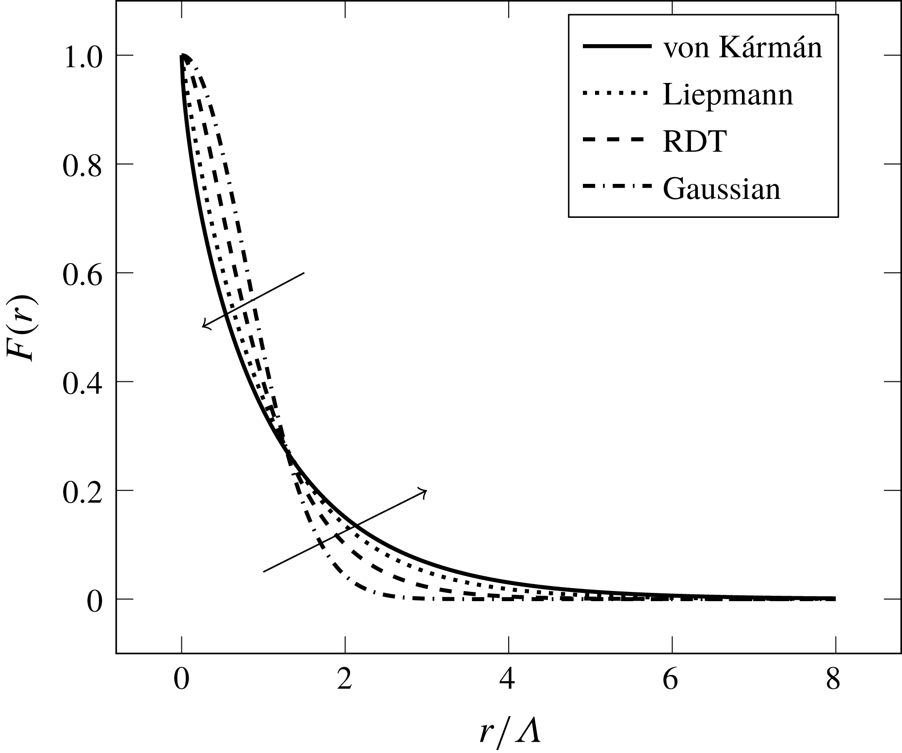
The longitudinal correlation functions presented in this section are depicted in figure 1. The correlation curves tend to drop faster to zero going from the Gaussian to the von Kármán function. Furthermore, according to (B 3), the integral of every curve for
 $r$
going from zero to infinity is equal to
 $\unicode[STIX]{x1D6EC}$
, so that the curves that go faster to zero show higher correlation values for small
 $r$
.
Analytical longitudinal correlation functions.

2.3.3 TNO-Blake model
The family of TNO-Blake models makes use of the von Kármán turbulence spectrum in order to compute the wall-pressure spectrum. However, the original TNO-Blake model (see Parchen Reference Parchen1998; Bertagnolio et al. Reference Bertagnolio, Fischer and Zhu2014) approximates the cross-spectrum of vertical velocity fluctuations as
 $$\begin{eqnarray}\unicode[STIX]{x1D711}_{22}(k_{1},x_{2},x_{2}^{\prime },k_{3})\approx L_{2}(x_{2})\,\unicode[STIX]{x1D711}_{22}^{a}(k_{1},x_{2},k_{3})\,\unicode[STIX]{x1D6FF}(x_{2}-x_{2}^{\prime })\,\unicode[STIX]{x1D6F7}_{m}(\unicode[STIX]{x1D714}-U_{c}(x_{2})k_{1}),\end{eqnarray}$$
where
 $L_{2}(x_{2})$
is a vertical correlation length scale, and
 $\unicode[STIX]{x1D6F7}_{m}$
is the so-called moving-axis spectrum, representing the contribution of the wavenumber
 $k_{1}$
to a given frequency
 $\unicode[STIX]{x1D714}$
. In most cases, Taylor’s hypothesis is applied and the moving-axis spectrum is expressed as
 $$\begin{eqnarray}\unicode[STIX]{x1D6F7}_{m}(\unicode[STIX]{x1D714}-U_{c}(x_{2})k_{1})=\unicode[STIX]{x1D6FF}(\unicode[STIX]{x1D714}-U_{c}(x_{2})k_{1}).\end{eqnarray}$$
The fundamental assumption behind the development of (2.29) is that
 $$\begin{eqnarray}R_{22}(r_{1},x_{2},x_{2}^{\prime },r_{3})=0\quad \text{for }x_{2}\neq x_{2}^{\prime },\end{eqnarray}$$
which can be hardly justified from a physical point of view. In fact, as will be shown later in § 4.3, the vertical velocity cross-correlation coefficient is not negligible over a vertical distance corresponding to at least two integral length scales. For this reason, Fischer et al. (Reference Fischer, Bertagnolio and Madsen2017) presented an improved version of the TNO-Blake model which corresponds to the substitution of the exact equation (2.25) (with
 $\unicode[STIX]{x1D708}=1/3$
) in (2.17). However, this hypothesis has the only advantage of reducing the number of dimensions of integration of the wall-pressure spectrum formulation. Then, the substitution of (2.29) and (2.30) in (2.17) yields the wavenumber wall-pressure spectrum,
 $$\begin{eqnarray}\unicode[STIX]{x1D711}_{pp}(\unicode[STIX]{x1D714}/U_{c},k_{3})\approx 8\,\unicode[STIX]{x1D70C}_{0}^{2}\int _{0}^{\infty }\frac{k_{1}^{2}}{k_{1}^{2}+k_{3}^{2}}\text{e}^{-2\sqrt{k_{1}^{2}+k_{3}^{2}}\,X_{2}}\left(\frac{\unicode[STIX]{x2202}U_{1}(x_{2})}{\unicode[STIX]{x2202}X_{2}}\right)^{2}L_{2}(X_{2})\,\unicode[STIX]{x1D711}_{22}^{a}(k_{1},X_{2},k_{3})\,\text{d}X_{2}.\end{eqnarray}$$
Finally, assuming equation (2.30), the corresponding frequency spectrum is calculated by coupling equation (2.32) with (2.18).
The treatment of the anisotropy of turbulence length scales in the TNO-Blake family of models is similar to that presented in (2.19). However, in this case there are three coefficients, representing the anisotropy of the length scales in the streamwise, wall-normal and transverse directions, respectively. The anisotropic three-dimensional auto-spectrum of vertical velocity fluctuations is
 $$\begin{eqnarray}\unicode[STIX]{x1D711}_{22}^{a,NI}(k_{1},k_{2},k_{3})=\unicode[STIX]{x1D6FD}_{1}\,\unicode[STIX]{x1D6FD}_{2}\,\unicode[STIX]{x1D6FD}_{3}\,\unicode[STIX]{x1D711}_{22}^{a,I}(\unicode[STIX]{x1D6FD}_{1}k_{1},\unicode[STIX]{x1D6FD}_{2}k_{2},\unicode[STIX]{x1D6FD}_{3}k_{3}).\end{eqnarray}$$
Integrating the previous equation in
 $\text{d}k_{2}$
yields the two-dimensional auto-spectrum used in (2.29)
 $$\begin{eqnarray}\unicode[STIX]{x1D711}_{22}^{a,NI}(k_{1},k_{3})=\unicode[STIX]{x1D6FD}_{1}\,\unicode[STIX]{x1D6FD}_{3}\,\unicode[STIX]{x1D711}_{22}^{a,I}(\unicode[STIX]{x1D6FD}_{1}k_{1},\unicode[STIX]{x1D6FD}_{3}k_{3}).\end{eqnarray}$$
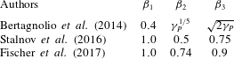
Various values for these coefficients have been proposed over time, as can be seen in table 1. The reason for the discrepancy in the values is that each set of parameters has been tuned empirically to a different experimental database. It can be noticed that Bertagnolio et al. (Reference Bertagnolio, Fischer and Zhu2014) expressed the vertical and transverse anisotropy coefficients as a function of the free-stream pressure gradient parameter
 $$\begin{eqnarray}\unicode[STIX]{x1D6FE}_{P}=\frac{\unicode[STIX]{x1D6FF}}{u_{\unicode[STIX]{x1D70F}}}\left[\frac{\text{d}P/\text{d}x_{1}}{\unicode[STIX]{x1D70C}_{0}\unicode[STIX]{x1D707}}\right],\end{eqnarray}$$
where
 $\text{d}P/\text{d}x_{1}$
is the gradient of the mean wall static pressure with respect to the abscissa along the aerofoil suction side. However, this dependence has been dropped in the later work of Fischer et al. (Reference Fischer, Bertagnolio and Madsen2017). None of the sets of coefficients presented in table 1 takes into account the variation of the anisotropy characteristics with the distance from the wall, a fact that is not negligible as will be shown in § 4.3.
Values of the anisotropy parameters
 $\unicode[STIX]{x1D6FD}_{i}$
according to different Authors.

The original TNO-Blake model is also characterised by the fact that the only flow quantity extracted from computational fluid dynamics (CFD) data is the mean shear, whereas the other quantities are defined with analytic expressions. These expressions can be found in Kamruzzaman et al. (Reference Kamruzzaman, Lutz, Würz, Shen, Zhu, Hansen, Bertagnolio and Madsen2012) and are here summarised. The vertical component of turbulent kinetic energy is
 $$\begin{eqnarray}\overline{u_{2}^{2}}=\unicode[STIX]{x1D6FC}_{0}\,k_{T},\end{eqnarray}$$
where
 $\unicode[STIX]{x1D6FC}_{0}=0.45$
on the suction side of an aerofoil and
 $0.35$
on the pressure side. The turbulent kinetic energy is modelled as a function of the mean shear
 $$\begin{eqnarray}k_{T}=\frac{\sqrt{\left(l_{mix}^{2}\left|{\displaystyle \frac{\unicode[STIX]{x2202}U_{1}}{\unicode[STIX]{x2202}x_{2}}}\right|{\displaystyle \frac{\unicode[STIX]{x2202}U_{1}}{\unicode[STIX]{x2202}x_{2}}}\right)^{2}}}{0.3}\end{eqnarray}$$
and
 $$\begin{eqnarray}l_{mix}=0.085\,\unicode[STIX]{x1D6FF}\,\tanh \left(\frac{0.41x_{2}}{0.085\,\unicode[STIX]{x1D6FF}}\right).\end{eqnarray}$$
In the last equation, the coefficient
 $0.41$
is the von Kármán constant. Finally, the integral length scale is
 $$\begin{eqnarray}\unicode[STIX]{x1D6EC}=\frac{l_{mix}}{0.41}.\end{eqnarray}$$
Equation (2.39) is used as an approximation of the vertical velocity correlation length
 $L_{2}(x_{2})$
.
2.4 A model of the turbulence–turbulence interaction wall-pressure spectrum
The derivation of a wavenumber-domain solution of the unsteady pressure generated by the turbulence–turbulence interaction source term, originally proposed by Hodgson (Reference Hodgson1961), is thoroughly reviewed and amended in some points in appendix C. In this section only the main hypotheses and the final expression are briefly recalled, referring to the appendix C for further considerations. The following assumptions are made:
(i) joint normal probability distribution of the turbulence at any two points across the boundary layer;
(ii) isotropic distribution of the turbulent kinetic energy in the three spatial coordinates
(2.40) $$\begin{eqnarray}\overline{u_{i}^{2}}(x_{2})=\overline{u^{2}}(x_{2})={\textstyle \frac{2}{3}}k_{T}(x_{2});\end{eqnarray}$$
(iii) cross-spectral density of velocity fluctuations having a Gaussian distribution in the wavenumber plane,
$\boldsymbol{k}$
: (2.41)where$$\begin{eqnarray}\unicode[STIX]{x1D711}_{ij}(x_{2},x_{2}^{\prime },\boldsymbol{k})=\frac{\overline{u^{2}}(x_{2})}{16\,\unicode[STIX]{x03C0}}\,L^{4}\,(k^{2}\unicode[STIX]{x1D6FF}_{ij}-k_{i}k_{j})\,\text{e}^{-\unicode[STIX]{x1D705}^{2}L^{2}/4}\,{\mathcal{F}}_{2},\end{eqnarray}$$
${\mathcal{F}}_{2}$
represents the vertical velocity correlation function: it can be assumed as Gaussian (C 32) or an exponential function (C 33); and(iv) negligible contribution of turbulence cross-spectral densities such that
$\unicode[STIX]{x1D711}_{i2}$
,
$i\in \{1,3\}$
.


Appendix C then shows that the following expression of the turbulence–turbulence wall-pressure PSD can be derived:
 $$\begin{eqnarray}\displaystyle \unicode[STIX]{x1D711}_{pp}^{TT}(\boldsymbol{k}) & = & \displaystyle \frac{\unicode[STIX]{x1D70C}_{0}^{2}\,L^{2}}{128\,\unicode[STIX]{x03C0}}\iint _{0}^{\infty }\overline{u^{2}}(X_{2})\,\overline{u^{2}}(X_{2}^{\prime })\,\text{e}^{-k(X_{2}+X_{2}^{\prime })}\,{\mathcal{F}}_{2}^{2}\,\text{d}X_{2}\,\text{d}X_{2}^{\prime }\nonumber\\ \displaystyle & & \displaystyle \times \,k^{2}\,(28+L^{2}k^{2})\,\text{e}^{-L^{2}k^{2}/8}.\end{eqnarray}$$
Equation (2.42) can be easily integrated with any numerical technique, being a two-dimensional integral. From this point of view, it can be compared with (2.4) to (2.7). In fact, Peltier & Hambric (Reference Peltier and Hambric2007) and Slama et al. (Reference Slama, Leblond and Sagaut2018) also made the assumption of a joint normal probability distribution of turbulence in order to treat the turbulence–mean shear and turbulence–turbulence interaction terms separately. Consequently, multiplying equation (2.7) by its complex conjugate in order to get the wall-pressure correlation coefficient yields a six-dimensional integral which must still be Fourier transformed in two dimensions in order to get the wavenumber PSD. However, the solution proposed in this section is derived at the price of some restrictive assumptions and should be seen as a means to better understand the relative importance of the two wall-pressure source components.
3 Heuristic investigation of the influence of the turbulent kinetic energy distribution
The previous section has highlighted the fact that the distribution of turbulent kinetic energy over the wavenumber spectrum can be represented by various analytical expressions. For this reason, the shape of a predicted wall-pressure PSD not only depends on the mean velocity and the r.m.s. vertical fluctuation profiles of the corresponding boundary layer, but also on the prescribed functional representation of the cross-spectrum of vertical fluctuations. The aim of this section is to make some heuristic considerations on the latter effect by using a simplified model of the boundary-layer profiles over a flat plate without a pressure gradient. This model, proposed by Kraichnan (Reference Kraichnan1956b ), assumes that the turbulent kinetic energy is constant in the vertical direction and that it is isotropic along the three axes, so that the r.m.s. velocity is
 $$\begin{eqnarray}\overline{u_{2}^{2}}(x_{2})=\overline{u^{2}}.\end{eqnarray}$$
Furthermore, the mean streamwise velocity gradient is assumed to decay exponentially with the wall-normal direction
 $$\begin{eqnarray}\frac{\unicode[STIX]{x2202}U_{1}}{\unicode[STIX]{x2202}x_{2}}=\frac{\unicode[STIX]{x1D70F}_{w}}{\unicode[STIX]{x1D707}}\text{e}^{-\unicode[STIX]{x1D6FE}x_{2}}.\end{eqnarray}$$
Kraichnan found that (3.2) is a fair approximation of the derivative of the logarithmic law of the wall if the parameter
 $\unicode[STIX]{x1D6FE}$
is of the order of magnitude of the inverse longitudinal integral length scale,
 $\unicode[STIX]{x1D6EC}$
. This is admittedly a highly artificial flow model and serves only as a first approximation towards the understanding of a real boundary layer, as the one treated in § 4, and its main advantage is merely its analytical simplicity. However, it will allow us to make some important considerations on the relationship between the model of turbulence statistics and the shape of the corresponding wall-pressure spectrum. For this purpose, all turbulence models discussed in § 2.3 will be used. In particular, the mathematical properties of the Gaussian and Liepmann models allow us to carry out analytically the integrations of (2.17). To begin with the Gaussian spectrum, substituting equations (2.22), (3.1), (3.2) in (2.17) and integrating with respect to
 $X_{2}$
and
 $X_{2}^{\prime }$
yields the following idealised wall-pressure spectral distribution:
 $$\begin{eqnarray}\unicode[STIX]{x1D711}(\boldsymbol{k})_{pp}^{TM}=\frac{\unicode[STIX]{x1D70C}_{0}^{2}\unicode[STIX]{x1D70F}_{w}^{2}\overline{u^{2}}L^{5}}{8\sqrt{\unicode[STIX]{x03C0}}\,\unicode[STIX]{x1D707}^{2}}\frac{k_{1}^{2}}{k+\unicode[STIX]{x1D6FE}}\text{e}^{(L^{2}/4)((k+\unicode[STIX]{x1D6FE})^{2}-k^{2})}\text{erfc}\left(\frac{L(k+\unicode[STIX]{x1D6FE})}{2}\right)\end{eqnarray}$$
(see § D.1 for the derivation).
Similarly, the substitution of (2.25) (with
 $\unicode[STIX]{x1D708}=1/2$
) and of (3.1) and (3.2) in (2.17) yields
 $$\begin{eqnarray}\unicode[STIX]{x1D711}(\boldsymbol{k})_{pp}^{TM}=\frac{\unicode[STIX]{x1D70C}_{0}^{2}\unicode[STIX]{x1D70F}_{w}^{2}\overline{u^{2}}\unicode[STIX]{x1D6EC}^{5}}{\unicode[STIX]{x03C0}\,\unicode[STIX]{x1D707}^{2}}\frac{k_{1}^{2}}{k+\unicode[STIX]{x1D6FE}}\frac{8(1+k^{2}\unicode[STIX]{x1D6EC}^{2})+9\,(k+\unicode[STIX]{x1D6FE})\unicode[STIX]{x1D6EC}\sqrt{1+k^{2}\unicode[STIX]{x1D6EC}^{2}}+3\,(k+\unicode[STIX]{x1D6FE})^{2}\unicode[STIX]{x1D6EC}^{2}}{(1+k^{2}\unicode[STIX]{x1D6EC}^{2})^{(5/2)}\left((k+\unicode[STIX]{x1D6FE})\unicode[STIX]{x1D6EC}+\sqrt{1+k^{2}\unicode[STIX]{x1D6EC}^{2}}\right)^{3}}\end{eqnarray}$$
(which is derived in § D.2). Equations (3.3) and (3.4) provide direct, if approximate, expressions of the wall-pressure energy distribution among the wavenumber spectrum which are a direct consequence of the respective assumptions on the energy distribution of the boundary-layer turbulence.
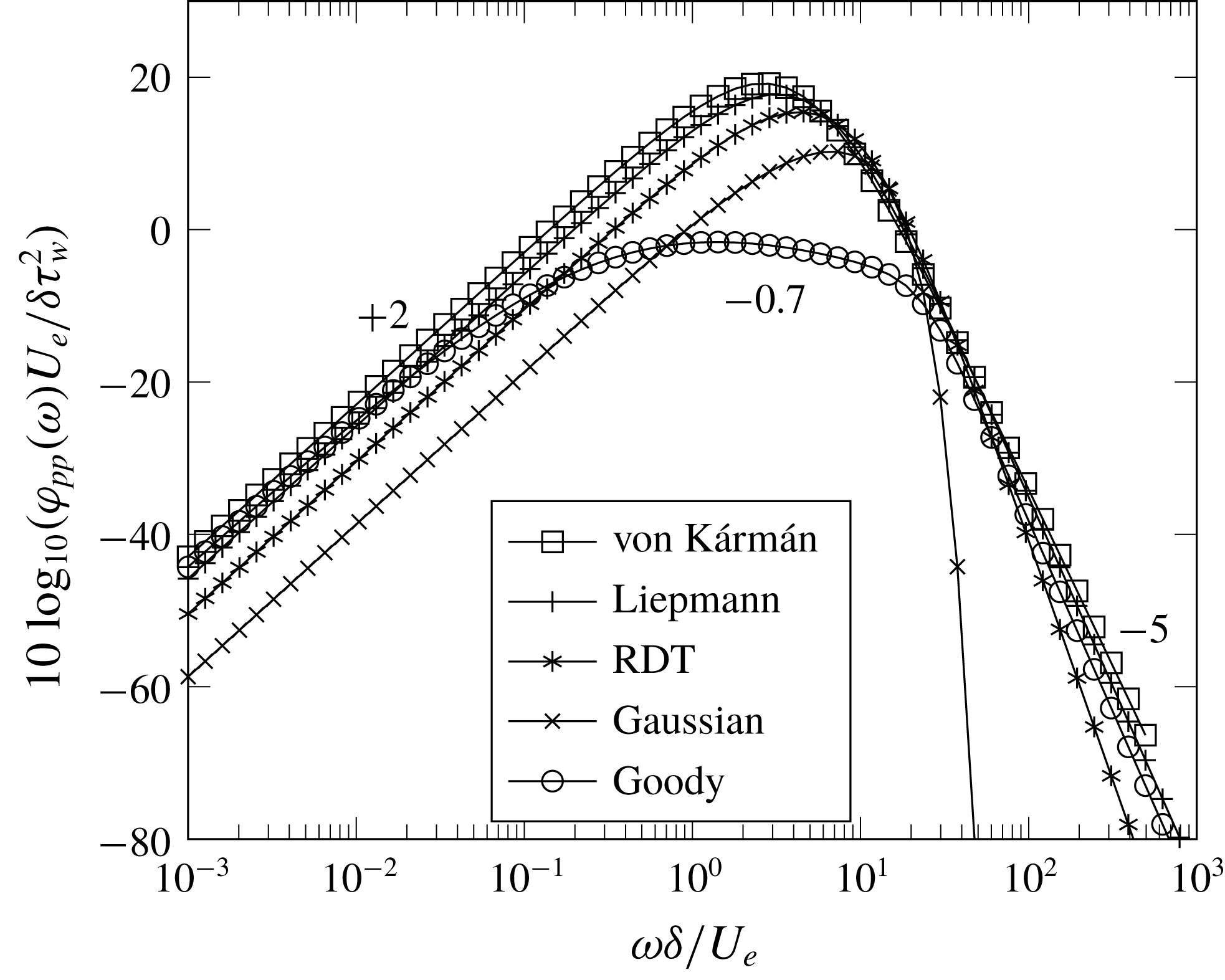
Comparison of Goody’s normalised wall-pressure frequency spectrum with the idealised spectral distribution derived from the Gaussian and Liepmann turbulence models.

3.1 Comparison with Goody’s model
The empirical model developed by Goody (Reference Goody2004) represents the basic physical features of a wall-pressure spectrum under a zero-pressure-gradient turbulent boundary layer. At the lower frequencies, which are dominated by larger-scale turbulent structures present in the outer part of the boundary layer, the spectrum rises as
 $\unicode[STIX]{x1D714}^{2}$
. The
 $\unicode[STIX]{x1D714}^{-0.7}$
decay corresponds to an overlap region that collapses with both inner and outer boundary-layer scaling parameters (see Goody Reference Goody2004). It has been argued that this region of the spectrum is mostly influenced by the physics of the log layer (see Bradshaw Reference Bradshaw1967). Finally, the wall-pressure spectrum decays as
 $\unicode[STIX]{x1D714}^{-5}$
for
 $\unicode[STIX]{x1D714}\rightarrow \infty$
(see also Moreau & Roger Reference Moreau and Roger2005, p. 49). These trends are represented in the equation
 $$\begin{eqnarray}{\displaystyle \frac{\unicode[STIX]{x1D711}_{pp}(\unicode[STIX]{x1D714})\,U_{0}}{\unicode[STIX]{x1D70F}_{w}^{2}\,\unicode[STIX]{x1D6FF}}}={\displaystyle \frac{3.0\,\left({\displaystyle \frac{\unicode[STIX]{x1D714}\,\unicode[STIX]{x1D6FF}}{U_{0}}}\right)^{2}}{\left[\left({\displaystyle \frac{\unicode[STIX]{x1D714}\,\unicode[STIX]{x1D6FF}}{U_{0}}}\right)^{0.75}+0.5\right]^{3.7}+\left[(1.1\,R_{T}^{-0.57})\,{\displaystyle \frac{\unicode[STIX]{x1D714}\,\unicode[STIX]{x1D6FF}}{U_{0}}}\right]^{7}}},\end{eqnarray}$$
where
 $$\begin{eqnarray}R_{T}=\left(\frac{u_{\unicode[STIX]{x1D70F}}\unicode[STIX]{x1D6FF}}{\unicode[STIX]{x1D708}}\right)\sqrt{\frac{C_{f}}{2}}\end{eqnarray}$$
represents the ratio of the outer layer to inner layer time scales. It can be noticed that the use of inner and outer boundary-layer parameters for normalisation provides a better overlap of different experimental curves over the whole frequency range (see Keith et al. Reference Keith, Hurdis and Abraham1992; Cipolla & Keith Reference Cipolla and Keith2000; Goody Reference Goody2004).
Equation (3.5) is compared with the distributions produced by the turbulence models of § 2.3, following the assumption that the main contribution to the wall-pressure spectrum is that of the turbulence–mean shear interaction. The results are depicted in figure 2. The Gaussian and Liepmann curves are obtained by means of (3.3) and (3.4), respectively. The wavenumber spectra given by these equations are transformed into frequency spectra by integrating numerically equation (2.18). The von Kármán and RDT curves are obtained by numerical integration of (2.17) and (2.18) in the
 $X_{2}$
,
 $X_{2}^{\prime }$
and
 $k_{3}$
variables. The following parameters, representative of a subsonic turbulent boundary layer at
 $M=0.2$
and
 $Re_{c}=5.85\times 10^{5}$
, have been used:
 $R_{T}=31.7$
,
 $U_{0}=68.0~\text{m}~\text{s}^{-1}$
,
 $U_{0}/U_{c}=1.25$
,
 $\overline{u^{2}}=4.16~\text{m}^{2}~\text{s}^{-2}$
,
 $\unicode[STIX]{x1D6FF}=3.38\times 10^{-3}~\text{m}$
,
 $\unicode[STIX]{x1D6EC}=0.473\times 10^{-3}~\text{m}$
,
 $\unicode[STIX]{x1D6FE}=1/(2\unicode[STIX]{x1D6EC})$
,
 $\unicode[STIX]{x1D70F}_{w}=11.8~\text{Pa}$
,
 $\unicode[STIX]{x1D707}=1.825\times 10^{-5}~\text{kg}~(\text{m}~\text{s})^{-1}$
and
 $\unicode[STIX]{x1D70C}_{0}=1.204~\text{kg}~\text{m}^{-3}$
. The results show that all turbulence models considered in this study are able to represent the quadratic rise of the wall-pressure PSD at low frequencies. In particular, the Liepmann and von Kármán curves are quite close to Goody’s in that range. Concerning the high-frequency range, only the Liepmann and von Kármán curves show a decay close to
 $\unicode[STIX]{x1D714}^{-5}$
, whereas the Gaussian curve drops much faster. Also the RDT curve drops slightly faster than the Liepmann and von Kármán ones. The
 $\unicode[STIX]{x1D714}^{-5}$
slope has been predicted theoretically by Blake (Reference Blake1986), who attributed it to the dominating influence of the viscous sub-layer. This is consistent with the fact that the Gaussian turbulence spectrum represents only large-scale turbulence structures, whereas the three turbulence spectral models classified under the generalised von Kármán spectrum take into account also the energy contained in the finer-scale structures such as those present in the viscous sub-layer. It is thus shown that the mere knowledge of the wavenumber distribution of turbulent kinetic energy, with only a simplified model of the boundary-layer mean and r.m.s. velocity profiles, is sufficient to justify the low-frequency and high-frequency slopes of the wall-pressure spectrum observed experimentally. On the contrary, the
 $\unicode[STIX]{x1D714}^{-0.7}$
slope of the overlap region cannot be retrieved by analytical considerations alone, at least not without a realistic model of the boundary-layer velocity profiles.
3.2 Effect on the mean-square wall pressure due to turbulence–mean shear interaction
The mean-square wall pressure due to the turbulence–mean shear interaction is defined as the integral of the wall-pressure PSD over the wavenumber spectrum
 $$\begin{eqnarray}\langle p^{2}\rangle _{TM}=\int _{\boldsymbol{k}}\unicode[STIX]{x1D711}_{pp}^{TM}(\boldsymbol{k})\,\text{d}\boldsymbol{k}.\end{eqnarray}$$
This integration can be performed analytically in order to understand how a given formulation of
 $\unicode[STIX]{x1D711}_{22}$
influences the predicted mean-square wall pressure, which is in turn directly proportional to the overall noise emitted by the trailing edge of an aerofoil, for instance. However, analytical solutions can be obtained only at the price of a further simplification, that is imposing
 $\unicode[STIX]{x1D6FE}=0$
. In this case, the mean shear would be constant across the boundary layer and the mean velocity profile would be linear. This is then representative only of the physics of the laminar sublayer of a turbulent boundary layer. The application of (3.6) to the Gaussian-based wall-pressure spectrum of (3.3) yields
 $$\begin{eqnarray}\langle p^{2}\rangle _{TM}=\frac{1}{3}\frac{\unicode[STIX]{x1D70C}_{0}^{2}\unicode[STIX]{x1D70F}_{w}^{2}\overline{u^{2}}L^{2}}{\unicode[STIX]{x1D707}^{2}}.\end{eqnarray}$$
Similarly, the integration of the Liepmann-based wall-pressure spectrum of (3.4) yields
 $$\begin{eqnarray}\langle p^{2}\rangle _{TM}=\frac{2}{3}\frac{\unicode[STIX]{x1D70C}_{0}^{2}\unicode[STIX]{x1D70F}_{w}^{2}\overline{u^{2}}\unicode[STIX]{x1D6EC}^{2}}{\unicode[STIX]{x1D707}^{2}}.\end{eqnarray}$$
It is thus verified that the flattening of the longitudinal correlation function of turbulence from a Gaussian to an exponential curve (see figure 1) makes the turbulence–mean shear interaction component of the mean-square wall pressure increase by a factor
 $2$
, within the assumptions of the simplified boundary-layer model and assuming that the length scales of the two turbulence models are equal. The same result was derived by Kraichnan (Reference Kraichnan1956a
) by integration of the wall-pressure correlation coefficient in the space domain. The study of a real boundary layer presented in § 4 will allow us to understand if this relationship between longitudinal correlation function and mean-square wall pressure holds also in the case of a real boundary layer.
3.3 Application to the turbulence–turbulence interaction component
Equation (2.42) can be integrated analytically in order to estimate the order of magnitude of the mean-square wall pressure due to the turbulence–turbulence source term of the Poisson equation. For illustrative purposes, the mean-square velocity
 $\overline{u^{2}}$
is considered constant in the
 $x_{2}$
direction. The result then depends on the choice of the
 ${\mathcal{F}}_{2}$
function. If the Gaussian function of (C 32) is substituted in (2.42) and the resulting formulation is integrated with respect to
 $X_{2}$
and
 $X_{2}^{\prime }$
, one obtains
 $$\begin{eqnarray}\unicode[STIX]{x1D711}_{pp}^{TT}(\boldsymbol{k})=\frac{\sqrt{2\unicode[STIX]{x03C0}}\unicode[STIX]{x1D70C}_{0}^{2}\,L^{3}\overline{u^{2}}^{2}}{512\,\unicode[STIX]{x03C0}}k\,(28+L^{2}k^{2})~\text{erfc}\left(\frac{\sqrt{2}}{4}kL\right).\end{eqnarray}$$
This result is obtained with a procedure similar to that described in § D.1. Then, the integration of (3.9) with respect to
 $\text{d}\boldsymbol{k}$
yields
 $$\begin{eqnarray}\langle p^{2}\rangle _{TT}=\frac{47}{30}\unicode[STIX]{x1D70C}_{0}^{2}\overline{u^{2}}^{2}\approx 1.57\unicode[STIX]{x1D70C}_{0}^{2}\overline{u^{2}}^{2}.\end{eqnarray}$$
If, on the contrary, the exponential function of (C 33) is substituted in (2.42), one obtains
 $$\begin{eqnarray}\displaystyle \unicode[STIX]{x1D711}_{pp}^{TT}(\boldsymbol{k}) & = & \displaystyle \frac{\unicode[STIX]{x1D70C}_{0}^{2}\,L^{2}}{128\,\unicode[STIX]{x03C0}}\iint _{0}^{\infty }\overline{u^{2}}(X_{2})\,\overline{u^{2}}(X_{2}^{\prime })\,\text{e}^{-k(X_{2}+X_{2}^{\prime })}\,\text{e}^{-\left|X_{2}-X_{2}^{\prime }\right|/L}\,\text{d}X_{2}\,\text{d}X_{2}^{\prime }\nonumber\\ \displaystyle & & \displaystyle \times \,k^{2}\,(28+L^{2}k^{2})\,\text{e}^{-L^{2}k^{2}/8}.\end{eqnarray}$$
In this case, the integral in
 $\text{d}X_{2}\,\text{d}X_{2}^{\prime }$
is solved by using the variable transformation
 $Y_{2}=X_{2}^{\prime }-X_{2}$
that yields
 $$\begin{eqnarray}\displaystyle & & \displaystyle \int _{0}^{\infty }\text{e}^{-kX_{2}}\,\text{d}X_{2}\int _{0}^{\infty }\text{e}^{-kX_{2}^{\prime }}\,\text{d}X_{2}^{\prime }~\text{e}^{-2\left|X_{2}-X_{2}^{\prime }\right|/L}\nonumber\\ \displaystyle & & \displaystyle \quad =\int _{0}^{\infty }\text{e}^{-2kX_{2}}\,\left(\int _{-X_{2}}^{\infty }\text{e}^{-kY_{2}}\text{e}^{-2\left|Y_{2}\right|/L}\,\text{d}Y_{2}\right)\,\text{d}X_{2}=\frac{L}{k(Lk+2)}\end{eqnarray}$$
for
 $Lk\neq -2$
(which is always verified because
 $L$
and
 $k$
are positive by definition). Then, substituting equation (3.12) in (2.42) leads to
 $$\begin{eqnarray}\unicode[STIX]{x1D711}_{pp}^{TT}(\boldsymbol{k})=\frac{\unicode[STIX]{x1D70C}_{0}\,L^{3}\,\overline{u^{2}}^{2}}{128\,\unicode[STIX]{x03C0}}\frac{k\,(28+L^{2}k^{2})}{(Lk+2)}\,\text{e}^{-L^{2}k^{2}/8},\end{eqnarray}$$
which corresponds to Hodgson’s equation (B.16) except that the present coefficient
 $28$
appears as
 $22$
in the manuscript, which is most likely a typewriting error. Finally, the integration of (3.13) with respect to
 $\text{d}\boldsymbol{k}$
yields
 $$\begin{eqnarray}\langle p^{2}\rangle _{TT}\approx 1.22\,\unicode[STIX]{x1D70C}_{0}^{2}\overline{u^{2}}^{2}.\end{eqnarray}$$
These considerations based on a simplified boundary-layer model suggest that the shape of the vertical correlation function does not alter significantly the mean-square wall pressure for constant
 $\overline{u^{2}}$
. Again, the application of the turbulence–turbulence interaction theory to the DNS data presented in § 4.6 will allow us to assess the validity of this result in case of a real boundary layer. It can also be noticed that the turbulence–turbulence mean-square wall pressure does not depend on the integral length scale, unlike the analogous expressions derived for the turbulence–mean shear component in § 3.2.
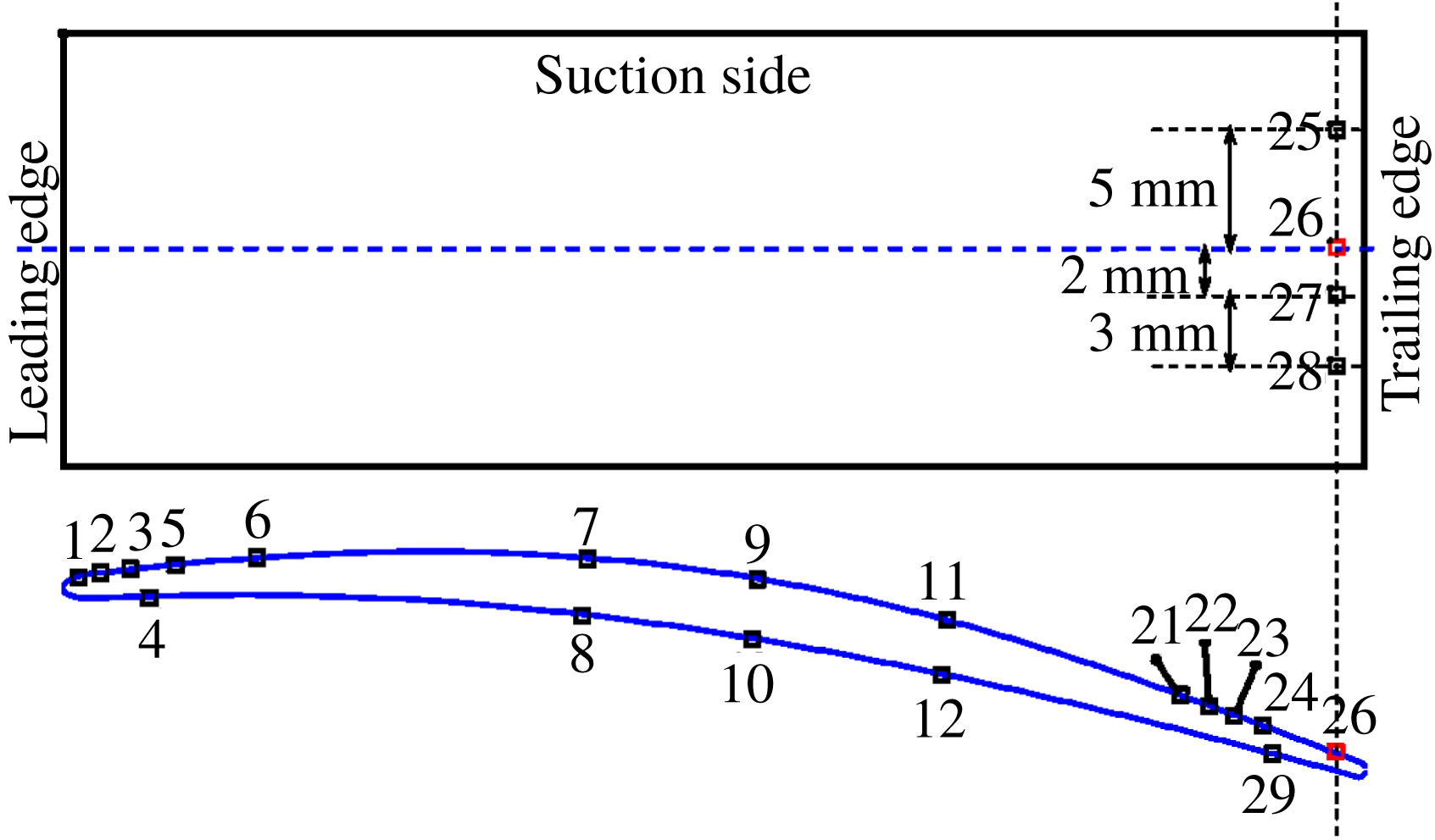
Distribution of wall-pressure sensors on the surface of the CD aerofoil.

4 Comparison of the models with direct numerical simulation and measurements of the flow over a controlled-diffusion aerofoil
4.1 Wall-pressure measurements
Measurements of the surface-pressure fluctuations on a controlled-diffusion (CD) aerofoil were performed in the anechoic open-jet wind tunnel at Université de Sherbrooke (see Padois et al. (Reference Padois, Laffay, Idier and Moreau2015) for an assessment of the capabilities of this facility for aeroacoustic investigations). The CD aerofoil is instrumented with remote microphone probes (RMP) on the suction side (see Moreau & Roger Reference Moreau and Roger2005). The RMPs are positioned along the streamwise and spanwise directions, as can be seen in figure 3. Each probe comprises a Knowles FG
 $23329$
P07 microphone remotely connected via a T junction to a pinhole of diameter of 0.5 mm on the suction side of the aerofoil and to a 2 m long anechoic termination on the other end to damp end reflections and avoid resonances (see for more details Perennes & Roger Reference Perennes and Roger1998). This microphone has a flat response in the frequency range of 100 to 10 kHz. For the calibration of the microphones a TMS microphone (130P10 ICP) with a diaphragm diameter equal to 6.35 mm was used. It is known to have a flat response in the frequency range of 100 to 20 kHz. The TMS microphone was calibrated using a Larson Davis 200 calibrator which has an uncertainty of approximately
 $\pm 0.2$
dB. The data were acquired using a NI 9234 module with a 24 bit resolution. The acquisition frequency was 25 600 Hz and the length of the signals was 30 s. Since the actual probes were not flush mounted but instead were placed at a remote location, this leads to attenuation of the surface pressure registered at the remote location. This attenuation can be attributed both to a change in section of the connecting tubes and the finite length of the tubing. Hence the actual signal measured by the remote microphone has an attenuated amplitude and is phase shifted. To account for these effects an in situ calibration procedure was realised.
Lastly, it should be kept in mind that, due to the finite size of the pinhole, some spatial averaging is anticipated especially at higher frequencies. Gravante et al. (Reference Gravante, Naguib, Wark and Nagib1998) performed a set of wall-pressure measurements with pinhole microphones of several diameters and showed that spectral attenuation can be avoided until
 $f^{+}=1$
if
 $12.0<d^{+}<18.0$
, where
 $f^{+}=f\,\unicode[STIX]{x1D708}_{T}/u_{\unicode[STIX]{x1D70F}}^{2}$
and
 $d^{+}=d\,u_{\unicode[STIX]{x1D70F}}/\unicode[STIX]{x1D708}_{T}$
are the frequency of interest and diameter of the pinhole respectively, both normalised by wall units. It was also shown that the diameter of the pinhole has no influence on the mean-square wall pressure up to
 $d^{+}=27$
. Using the friction velocity calculated from the DNS, the
 $d^{+}$
for sensor
 $21$
was estimated to be equal to
 $26.0$
, whereas
 $d^{+}$
for sensor
 $24$
was estimated to be equal to
 $22.2$
. Likewise,
 $f^{+}=1$
corresponds to
 $f=39.1$
kHz for sensor 21 and to
 $f=28.6$
kHz for sensor 24. However, since the measurement range for the Knowles FG
 $23329$
P
 $07$
is restricted to
 $10$
kHz the attenuation effects are expected to be small. However, Roger (Reference Roger2017) has shown with analytical considerations that the attenuation due to integration effects at high frequencies depends on the statistical properties of the wall-pressure field to be measured. Then, the DNS-based wall-pressure statistics could be used in the future to understand better this effect.
4.2 DNS of the flow over the controlled-diffusion aerofoil
The three-dimensional DNS of the flow over the CD aerofoil is conducted using a multi-block structured high-order accurate compressible Navier–Stokes solver (Sandberg Reference Sandberg2015) taking the mean installation effects ( jet width) into account, as suggested by Moreau et al. (Reference Moreau, Henner, Iaccarino, Wang and Roger2003). The volume data around the aerofoil were recorded during the simulation at a sampling frequency of 78 kHz for 7 flow-through times based on the reference velocity and aerofoil chord length, which was found enough to yield properly converged flow statistics in previous large-eddy simulations (LES) and DNS on this aerofoil at this flow condition (see Wang et al.
Reference Wang, Moreau, Iaccarino and Roger2009; Moreau et al.
Reference Moreau, Sanjosé, Perot and Kim2011; Wu, Moreau & Sandberg Reference Wu, Moreau and Sandberg2019). A fourth-order central standard-difference scheme with Carpenter boundary stencils (Carpenter, Nordström & Gottlieb Reference Carpenter, Nordström and Gottlieb1999) is applied for the spatial discretisation in the streamwise and cross-wise directions. A spectral method using the FFTW3 library is used in the spanwise direction. Time marching is achieved by an ultra-low-storage five-step fourth-order Runge–Kutta scheme (Kennedy, Carpenter & Lewis Reference Kennedy, Carpenter and Lewis1999) with a constant time step of
 $\unicode[STIX]{x0394}t=6.4\times 10^{-8}$
s. Characteristic-based boundary conditions (described in Sandberg & Sandham Reference Sandberg and Sandham2006; Jones Reference Jones2008; Jones, Sandberg & Sandham Reference Jones, Sandberg and Sandham2008) (see also Kim & Lee Reference Kim and Lee2003) are used for this simulation on domain boundaries to avoid unphysical reflections (see for more details Wu et al.
Reference Wu, Sanjosé, Moreau and Sandberg2018). An adiabatic, no-slip condition is set on the aerofoil surface. The grid refinement in the boundary layers is guided by the data obtained from experiments (Moreau et al.
Reference Moreau, Henner, Iaccarino, Wang and Roger2003; Wu et al.
Reference Wu, Laffay, Idier, Jaiswal, Sanjosé and Moreau2016). In the spanwise direction, 96 Fourier modes are employed with 100 % de-aliasing, which corresponds to 194 collocation points in physical space. These points are distributed with equal distance over a spanwise width of 12 % of the aerofoil chord length and are shown to resolve properly the Kolmogorov scale (see Wu et al.
Reference Wu, Sanjosé, Moreau and Sandberg2018, Reference Wu, Moreau and Sandberg2019). The O-grid around the boundary layer comprises
 $3341\times 279\times 194$
grid points, which give finally a grid resolution of
 $\unicode[STIX]{x0394}x_{1,ave}^{+}\approx 6.0$
,
 $\unicode[STIX]{x0394}x_{2,ave}^{+}\approx 0.8$
and
 $\unicode[STIX]{x0394}x_{3,ave}^{+}\approx 5.5$
based on the friction velocity. These average values are calculated on the rear part of the aerofoil surface corresponding to 40 % of the aerofoil chord. Further details on the validation of the DNS can be found in Wu et al. (Reference Wu, Moreau and Sandberg2019) including turbulent kinetic energy budgets.
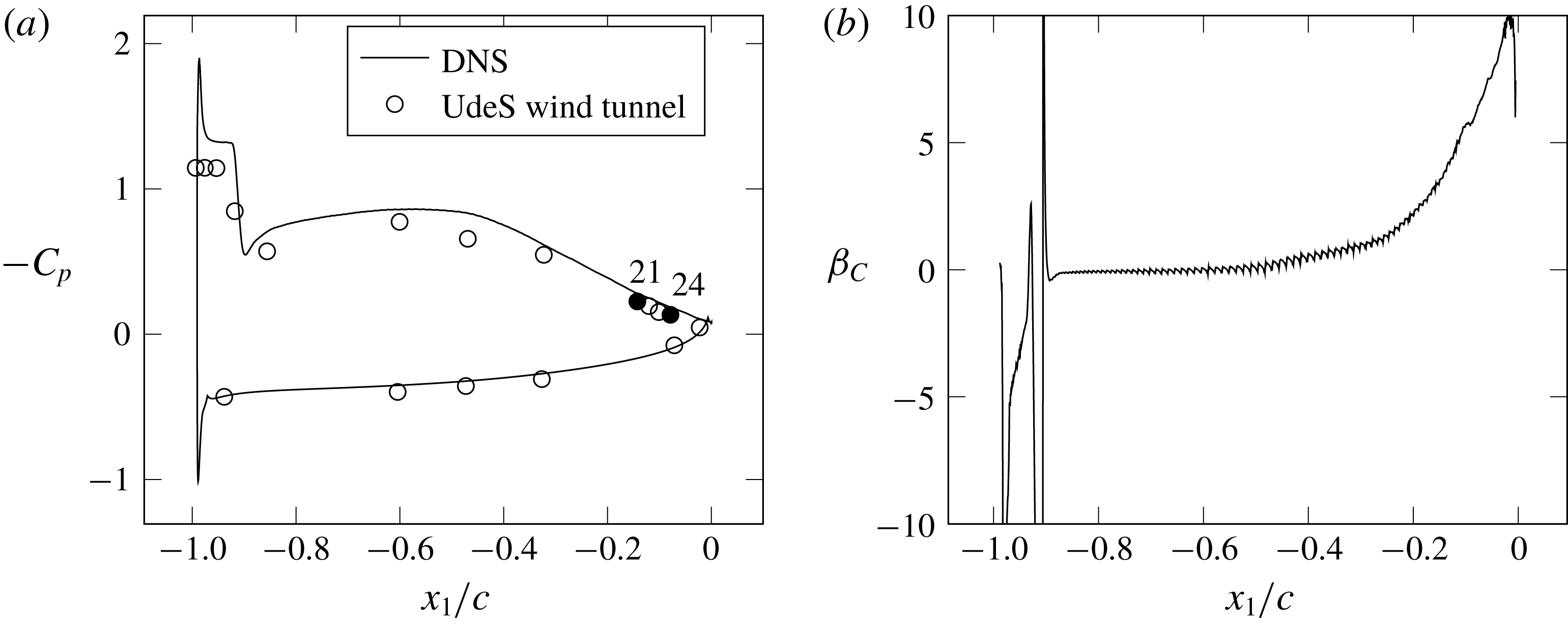
(a) Comparison of the measured and DNS pressure coefficient,
 $C_{p}$
. (b) Clauser parameter,
 $\unicode[STIX]{x1D6FD}_{c}$
, calculated from the DNS results.

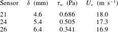
Parameters for the normalisation of frequency and wall-pressure PSD.

Mean velocity profiles extracted from the DNS data on the aerofoil surface and in the wake compare favourably with hot-wire measurements performed in the anechoic wind tunnel of the Université de Sherbrooke (UdeS) (see Wu et al. Reference Wu, Sanjosé, Moreau and Sandberg2018, Reference Wu, Moreau and Sandberg2019). The calculated pressure coefficient,
 $$\begin{eqnarray}C_{p}=\frac{p-p_{0}}{1/2\,\unicode[STIX]{x1D70C}_{0}\,U_{e}^{2}},\end{eqnarray}$$
where
 $p_{0}$
is the free-stream static pressure, is compared in figure 4(a) with wall-pressure measurements taken in the same wind tunnel, which has a free-stream turbulence intensity below 0.4 %. A laminar separation bubble can be observed at the leading edge, whose extension is well captured by the DNS. The onset of an adverse pressure gradient is visible on the rear half of the suction side. The development of the pressure gradient on the suction side of the aerofoil is presented in figure 4(b) using the Clauser parameter, defined as,
 $$\begin{eqnarray}\unicode[STIX]{x1D6FD}_{C}=\frac{\unicode[STIX]{x1D6FF}^{\ast }}{\unicode[STIX]{x1D70F}_{w}}\frac{\text{d}P}{\text{d}x_{1}}.\end{eqnarray}$$
The pressure gradient with respect to the abscissa along the aerofoil,
 $\text{d}P/\text{d}x_{1}$
, increases continuously from the mid-chord to the trailing edge.
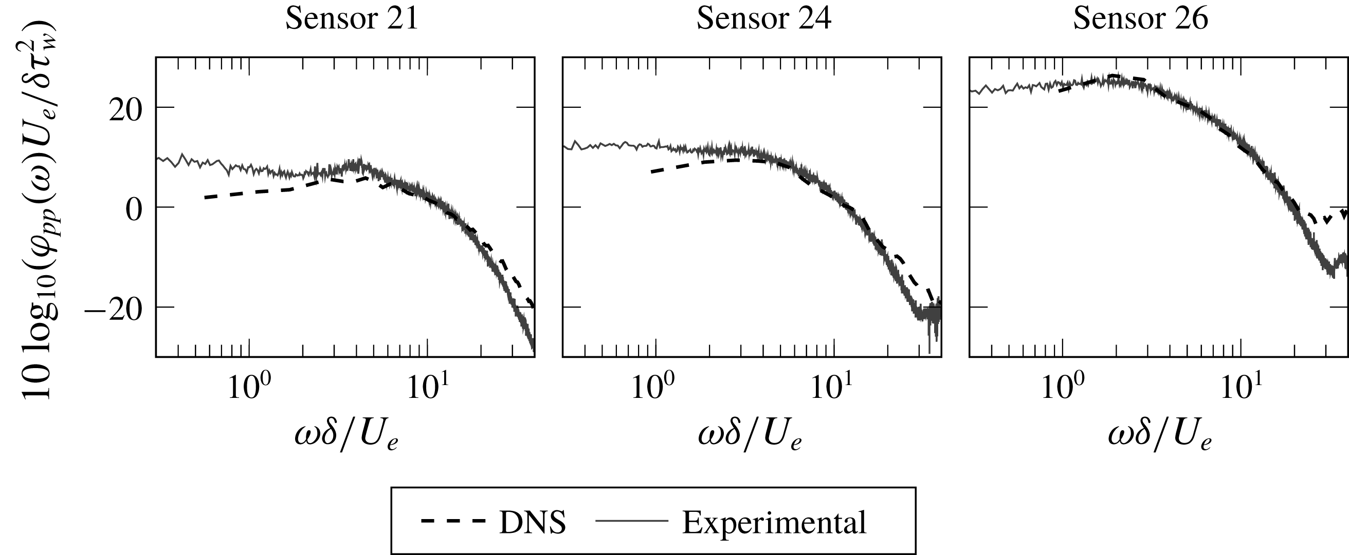
The wall-pressure PSD calculated from the DNS results is compared in figure 5 with the measured one at three pressure sensors on the suction side of the aerofoil close to the trailing edge, namely sensor 21 (with
 $\unicode[STIX]{x1D6FD}_{C}=5.01$
), sensor 24 (with
 $\unicode[STIX]{x1D6FD}_{C}=6.28$
) and sensor 26 (with
 $\unicode[STIX]{x1D6FD}_{C}=9.72$
). The boundary-layer parameters used for the normalisation of the curves are summarised in table 2. The boundary-layer thickness corresponds to the
 $x_{2}$
coordinate where the total pressure reaches 99 % of its maximum constant value along the wall-normal direction. The total pressure is used instead of the velocity because the aerofoil is loaded and therefore the external flow is deflected so that the external velocity is not constant. It can be noticed that at the lower frequencies the DNS spectrum is slightly below the experimental one. This is due to the fact that, whereas the simulation does not include the jet unsteadiness and acoustics, some significant effect from the jet is inevitable in the experiment, which prevents us obtaining the theoretical positive slope in the wall-pressure spectra. In the case of sensor 26, a high-frequency hump can be noticed, which is attributed to the contamination from the acoustic sources in the wake of the aerofoil. For this reason, the following analysis will focus on sensors 21 and 24 only.
Comparison of the measured and DNS calculated wall-pressure PSD,
 $\unicode[STIX]{x1D711}_{pp}$
, on the suction side of the CD aerofoil corresponding to the locations of three pressure sensors.

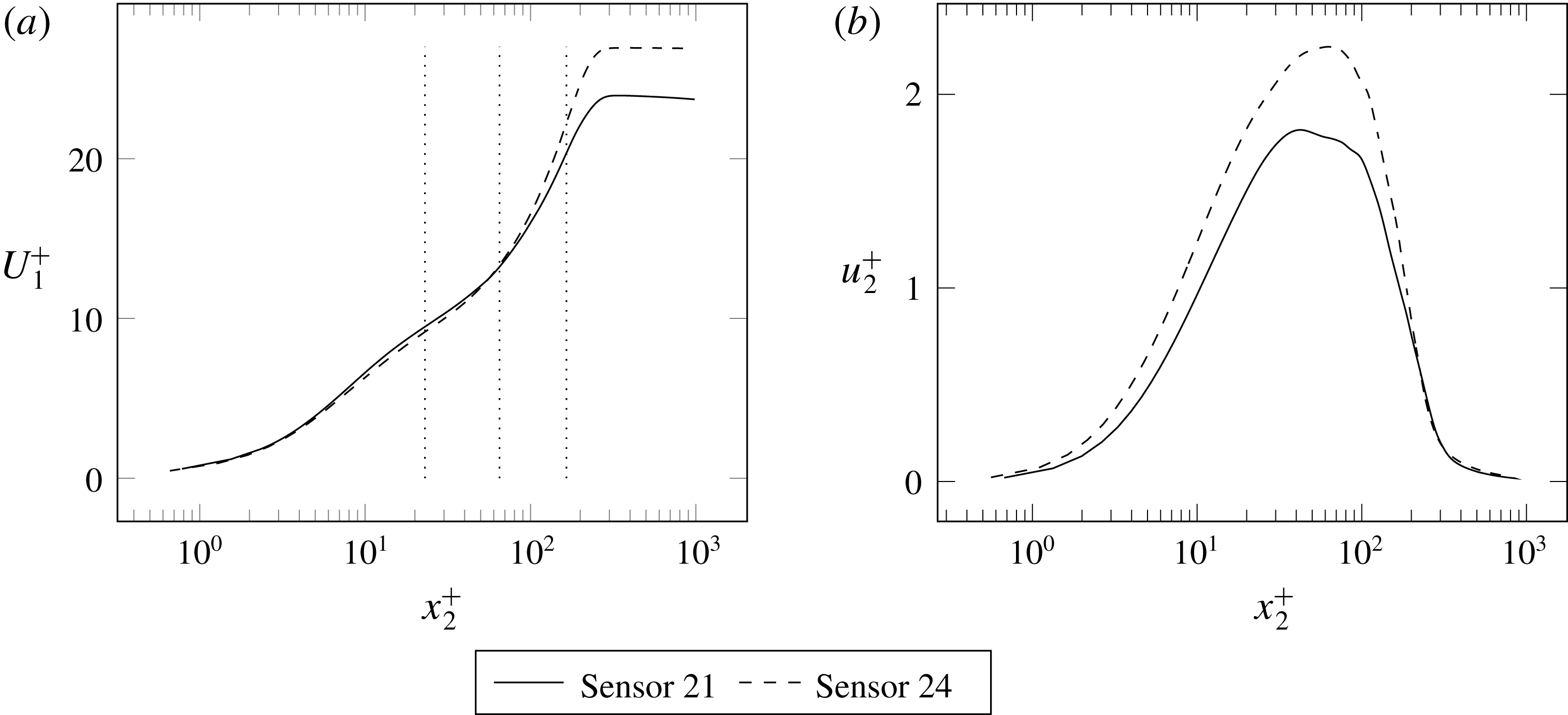
Normalised boundary-layer profiles extracted from the averaged DNS flow field corresponding to pressure sensors 21 and 24, respectively. (a) Mean streamwise velocity; (b) r.m.s. vertical velocity. The dotted lines on (a) indicate the locations chosen for the calculation of turbulence cross-correlation coefficients.

Finally, figure 6 presents the boundary-layer profiles of mean streamwise velocity and vertical r.m.s. fluctuation extracted from the DNS corresponding to sensors 21 and 24. Both plots are normalised in wall units. The effect of the increase of
 $\unicode[STIX]{x1D6FD}_{C}$
from sensors 21 to 24 can be observed in the mean velocity plot of figure 6(a), particularly in the wake zone of the boundary layer corresponding to
 $x_{2}^{+}>100$
. Also the vertical r.m.s. fluctuation of figure 6(b) is seen to increase with the Clauser parameter as expected.
4.3 Calculation of turbulence statistics
The DNS of the flow around the CD aerofoil is post-processed to gain information on the statistics of turbulence that are part of the above analytical model for the prediction of the wall-pressure spectrum. The wall-normal velocity correlation coefficient,
 $R_{22}$
, is analysed. In fact, the cross-spectral density of wall-normal velocity fluctuations,
 $\unicode[STIX]{x1D711}_{22}$
, which appears in (2.17), is the double spatial Fourier transform of
 $R_{22}$
(see (B 9)). The correlation coefficients calculated from the DNS results are compared with the analytical formulations that are derived from a given longitudinal correlation function,
 $F(r)$
, according to (B 6). This comparison assesses the accuracy of the analytical formulation of
 $\unicode[STIX]{x1D711}_{22}^{I}$
. The
 $R_{22}$
profiles discussed below are extracted from planes parallel to the suction side of the CD aerofoil using seven flow-through times for averaging. The results correspond to sensor 24. The same calculations performed for sensor 21 are not reported here for brevity as they yield equivalent results. The profiles are plotted versus the distance from the reference point,
 $r$
, normalised by the longitudinal integral length scale,
 $\unicode[STIX]{x1D6EC}$
, calculated at each wall-normal position. Furthermore,
 $R_{22}$
is calculated for several streamwise,
 $r_{1}$
, and transverse
 $r_{3}$
separations. The curves of
 $R_{22}(r_{1})$
and
 $R_{22}(r_{3})$
nearly collapse if the coordinate
 $r_{1}$
is divided by the coefficient
 $\unicode[STIX]{x1D6FC}$
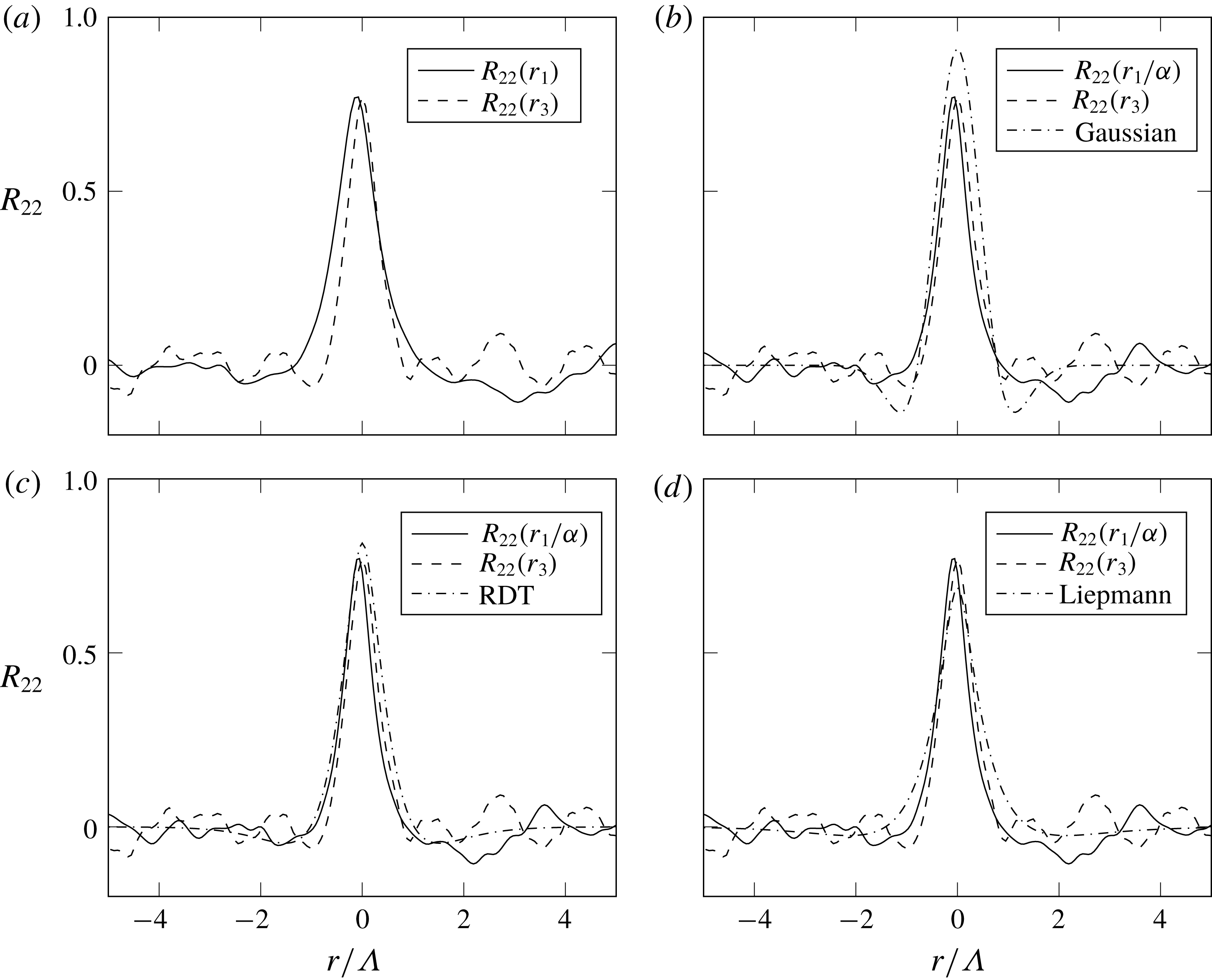
that represents the ratio of streamwise to transverse longitudinal integral length scales (see (2.19)).
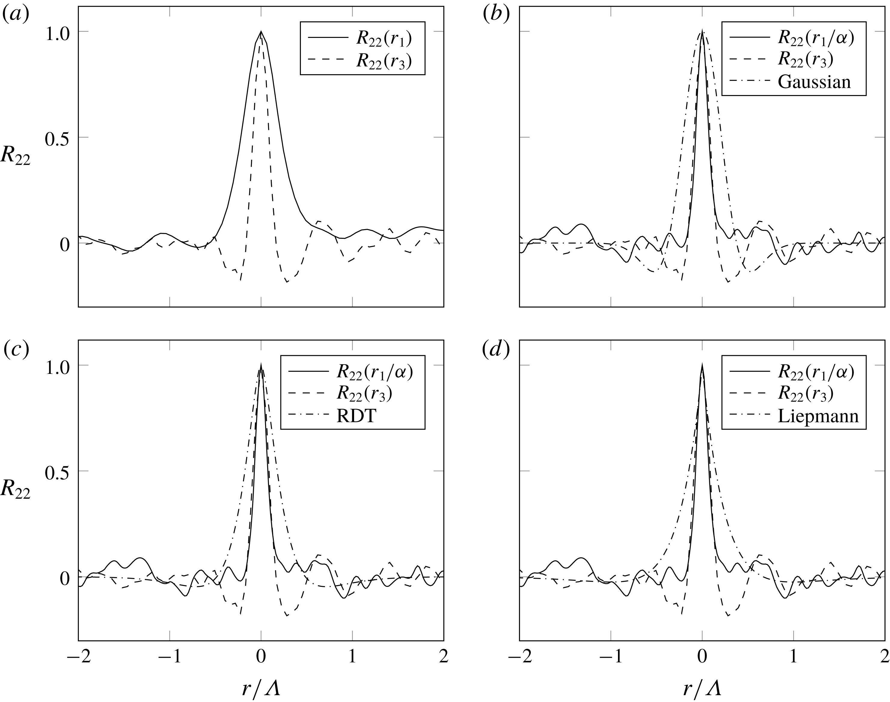
Vertical velocity correlation coefficient calculated on a plane at
 $x_{2}^{+}=23$
in the streamwise (
 $r_{1}$
) and transverse (
 $r_{3}$
) directions. Ratio of streamwise to transverse length scales:
 $\unicode[STIX]{x1D6FC}=1.88$
.

Figure 7(a) shows the
 $R_{22}(r_{1})$
and
 $R_{22}(r_{3})$
profiles extracted from a plane at
 $x_{2}^{+}=23$
. In this case, it is sufficient to take
 $\unicode[STIX]{x1D6FC}=1.88$
for the curves to coincide, at least for small separations,
 $r$
. The transverse correlation
 $R_{22}(r_{3})$
is higher than
 $R_{22}(r_{1})$
for longer separations, whereas
 $R_{22}(r_{1})$
exhibits negative lobes. These facts point to the presence of coherent turbulent structures elongated in the transverse direction (see Sillero, Jiménez & Moser Reference Sillero, Jiménez and Moser2014, figure 1). Wu et al. (Reference Wu, Sanjosé, Moreau and Sandberg2018) have shown that the onset of these structures is related to the increase of the adverse pressure gradient and that also the wall-pressure correlation coefficient increases in the transverse direction. In this case, all analytical formulations seem to overestimate the numerical correlation coefficients. Only the Liepmann formulation is in close agreement with the numerical curves for small values of
 $r$
. The von Kármán formulation is not shown in this analysis as its results are very close to that of Liepmann in all calculations.
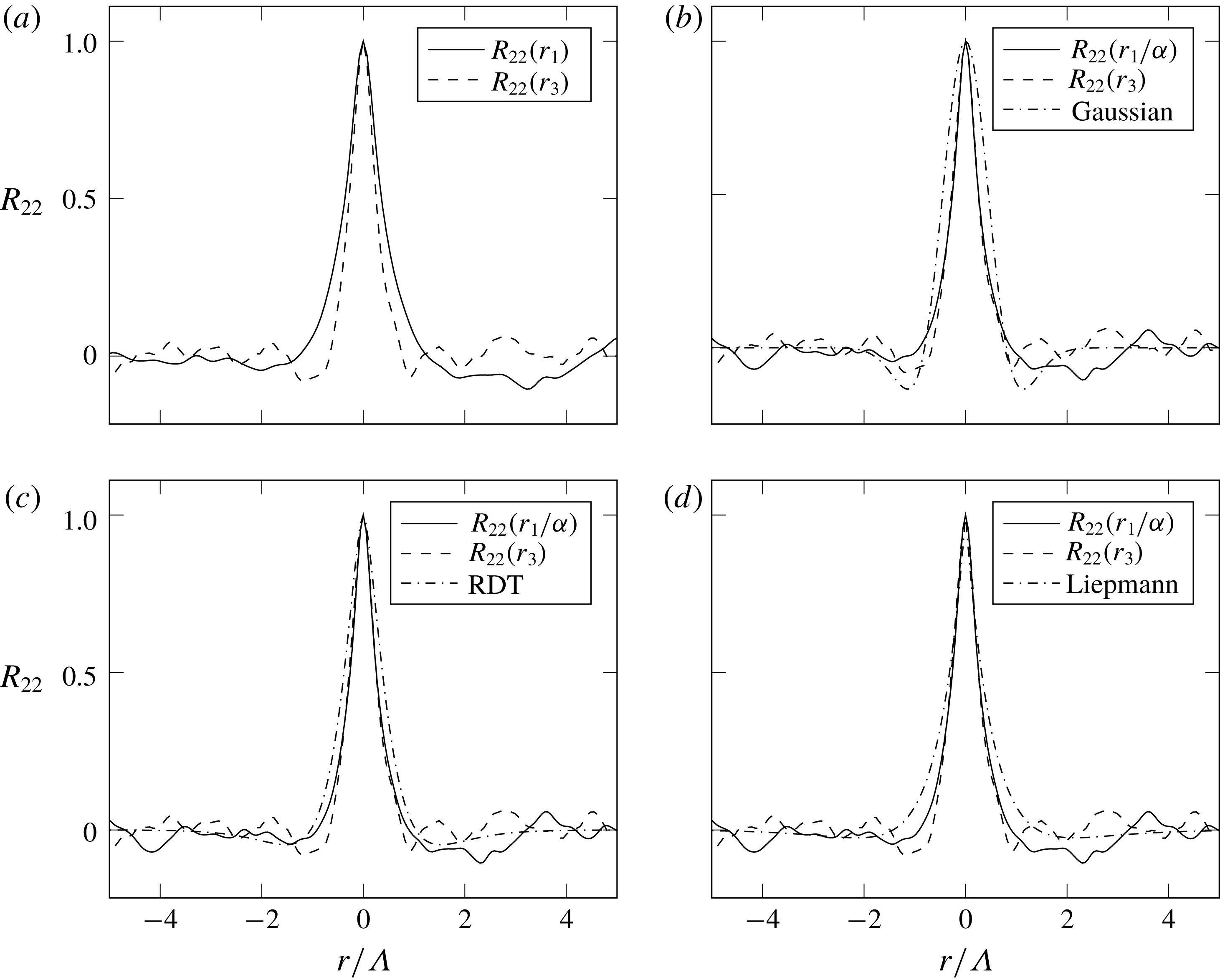
Vertical velocity correlation coefficient calculated on a plane at
 $x_{2}^{+}=65$
in the streamwise (
 $r_{1}$
) and transverse (
 $r_{3}$
) directions. Ratio of streamwise to transverse length scales:
 $\unicode[STIX]{x1D6FC}=1.55$
.

Figure 8 presents the same analysis of the velocity fluctuations extracted from a plane at
 $x_{2}^{+}=65$
. The elongation of the turbulence structures farther away from the wall is represented by the coefficient
 $\unicode[STIX]{x1D6FC}=1.55$
. In this case, the Gaussian formulation overestimates the negative undershoots of the numerical curves. On the contrary both the RDT and the Liepmann formulations give good approximations to the results. In particular, the Liepmann curve is closer to the computed
 $R_{22}$
for
 $r<1$
, whereas for
 $r>1$
the RDT curve is the closest.
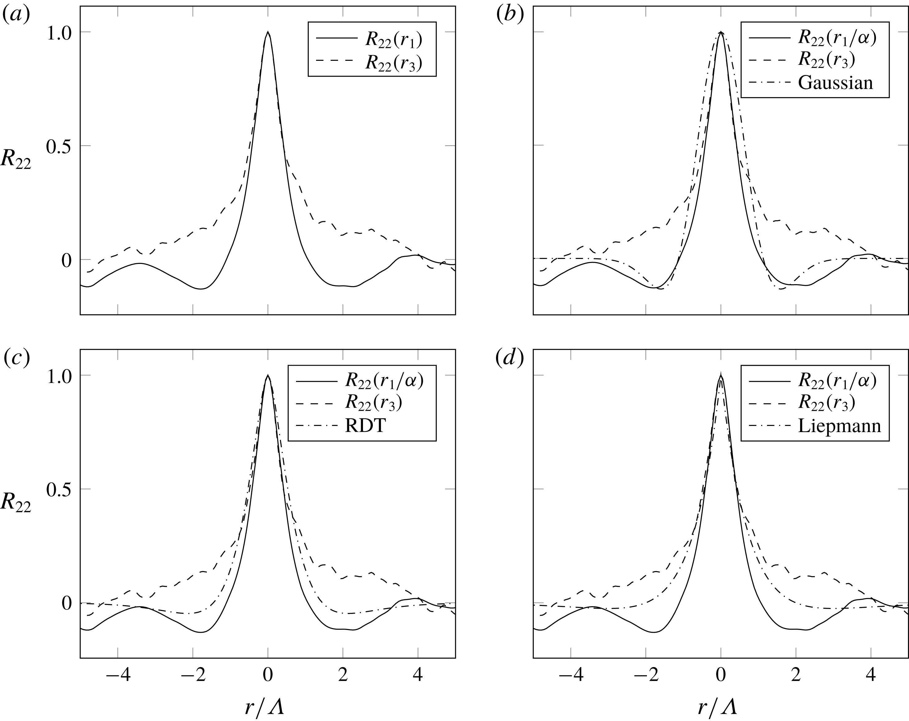
Vertical velocity correlation coefficient calculated on a plane at
 $x_{2}^{+}=165$
in the streamwise (
 $r_{1}$
) and transverse (
 $r_{3}$
) directions. Ratio of streamwise to transverse length scales:
 $\unicode[STIX]{x1D6FC}=1.35$
.

Figure 9 refers to a plane close to the outer edge of the boundary layer (
 $x_{2}^{+}=165$
), where the elongation of the turbulent structures is
 $\unicode[STIX]{x1D6FC}=1.35$
. It can be noticed that the Gaussian theory (figure 9
b) reproduces well the negative parts of the curve of
 $R_{22}$
. Figures 9(c) and 9(d) compare the DNS curves with the RDT and Liepmann formulations, respectively. In this case, the former analytical formulation provides a slightly better representation of the numerical results than the latter.
In the results presented so far it has been assumed that
 $\unicode[STIX]{x0394}x_{2}=0$
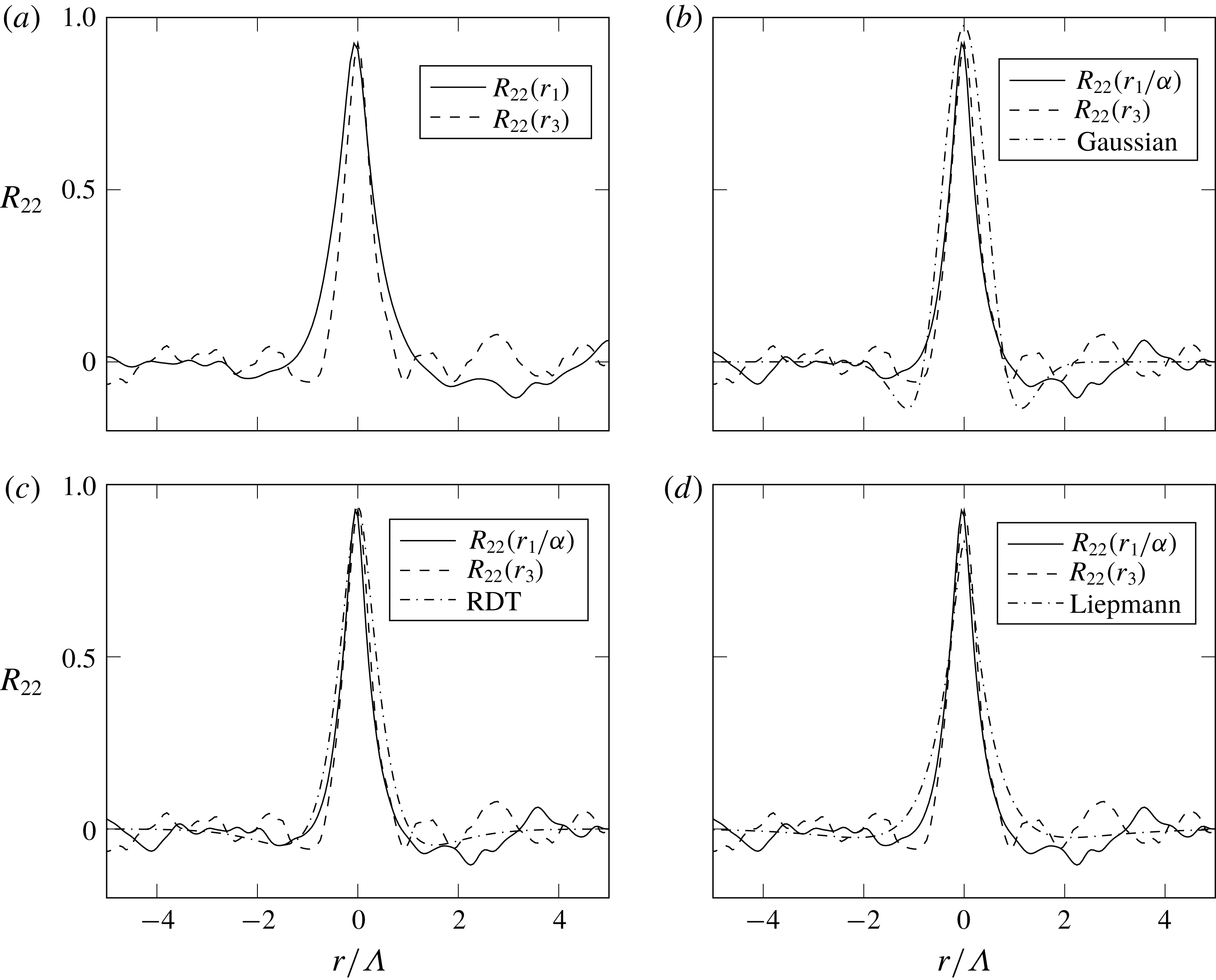
. In order to complete this analysis, the calculation of
 $R_{22}$
between two planes parallel to the wall is now presented. Figure 10 shows the correlation coefficient computed between the plane at
 $x_{2}^{+}=65$
and a second plane parallel to the wall which has a normalised distance
 $\unicode[STIX]{x0394}x_{2}/\unicode[STIX]{x1D6FF}=0.024$
from the first. Due to the wall-normal separation, the maximum value of
 $R_{22}$
, found at
 $r_{1}=r_{3}=0$
, is logically lower than unity. Visibly, the three analytical formulations predict differently the decay of
 $R_{22}$
with
 $\unicode[STIX]{x0394}x_{2}$
. In this case, the RDT and Liepmann formulations are in better agreement with the numerical data than the Gaussian. Finally, figure 11 presents the
 $R_{22}$
coefficient calculated between the plane at
 $x_{2}^{+}=65$
and another plane at
 $\unicode[STIX]{x0394}x_{2}/\unicode[STIX]{x1D6FF}=0.05$
from the first. It can be noticed that the peak of
 $R_{22}(r_{1})$
corresponds to a
 $r_{1}$
slightly below zero, whereas the plot of
 $R_{22}(r_{3})$
is centred on
 $r_{3}=0$
. This is due to the fact that the velocity time series has been extracted directly at the mesh cell centres, in order to avoid the numerical error introduced by interpolation. The mesh follows the curvature of the aerofoil surface, so the cell centres are not perfectly aligned in the wall-normal direction, whereas there is perfect alignment in the transverse direction. It must be emphasised that if the fundamental assumption of the TNO-Blake model, expressed in (2.31), was true, then the DNS-based statistics presented in figures 10 and 11 would vanish for any
 $r$
.
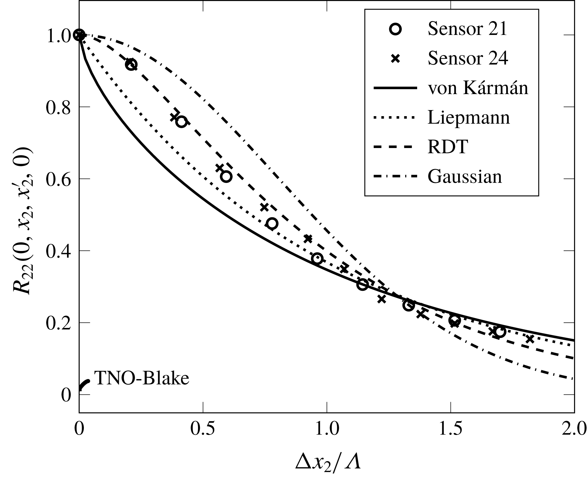
The decay of the maximum
 $R_{22}$
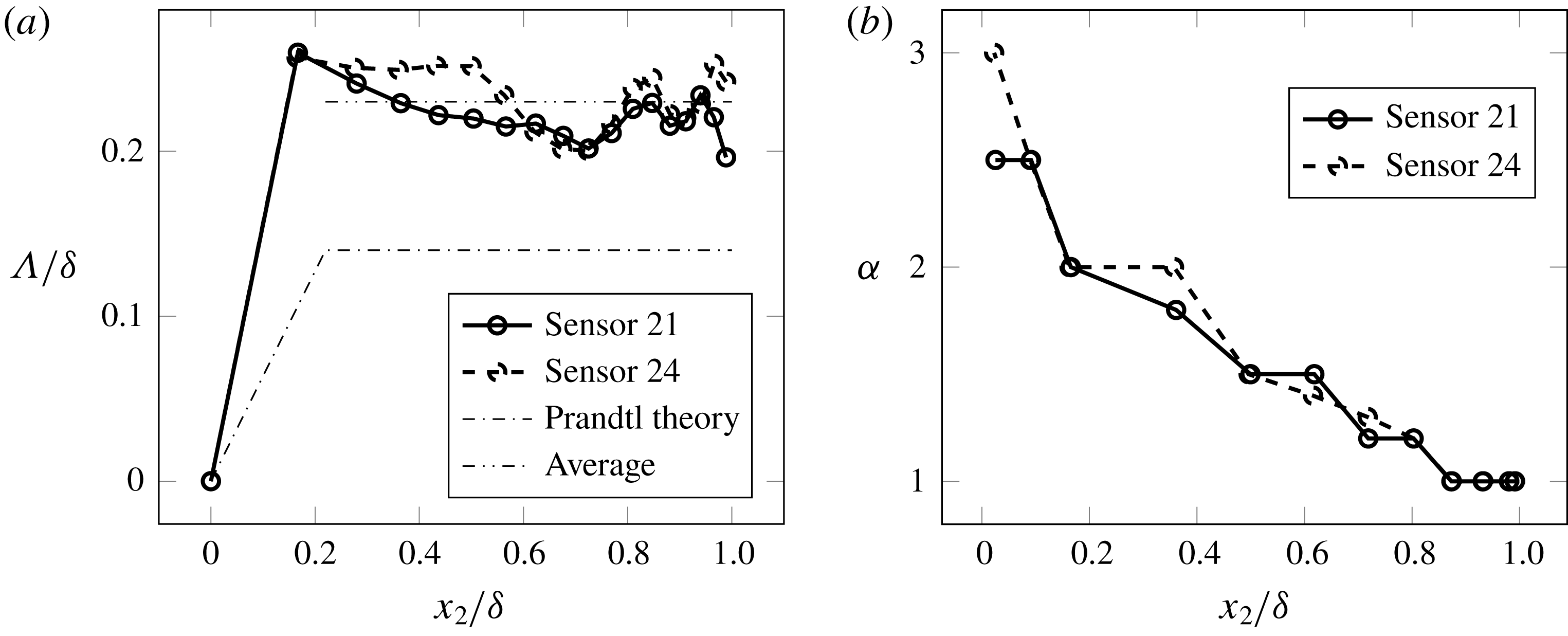
with the increase of the vertical separation is plotted in figure 12. The reference point for this calculation has been taken at roughly half the boundary layer thickness for both sensors 21 and 24. The second point for the calculation of the cross-correlation coefficient has been chosen moving upwards in the vertical direction. As will be shown below, the longitudinal integral length scale of turbulence is nearly constant in this region of the boundary layer. For this reason, it has been possible to normalise the abscissa of figure 12 using the averaged
 $\unicode[STIX]{x1D6EC}$
in the outer part of the boundary layer. It can be observed that, especially for small separations, the RDT is in best agreement with the DNS data corresponding to both sensors. For higher vertical separations, the DNS data are between the RDT and Liepmann theoretical curves. The cross-correlation coefficient of vertical velocity fluctuations is significantly higher than zero on a vertical extension corresponding to two integral length scales, thus further contradicting equation (2.31).
The general conclusion that can be drawn from this study is that especially the RDT and, second, the Liepmann models provide an acceptable description of the turbulence statistics in this adverse-pressure-gradient boundary layer. The present result is also very consistent with what Magnaudet (Reference Magnaudet2003) found: the rapid distortion theory is the leading-order approximation capable of describing short- and long-time evolutions of turbulent boundary layers in the limit of large Reynolds number. In any case, all analytical formulations of the cross-spectral density of wall-normal turbulent fluctuations,
 $\unicode[STIX]{x1D711}_{22}$
, that have been presented in § 2.3 will be applied to the prediction of the wall-pressure spectra on the surface of the CD aerofoil in § 4.5. In this way, the relationship between the shape of turbulence statistics and that of the corresponding wall-pressure PSD will be assessed.
Vertical velocity correlation coefficient calculated between a reference plane at
 $x_{2}^{+}=65$
and a second plane parallel to the wall at
 $\unicode[STIX]{x0394}x_{2}/\unicode[STIX]{x1D6FF}=0.024$
from the first. Ratio of streamwise to transverse length scales:
 $\unicode[STIX]{x1D6FC}=1.55$
.

Vertical velocity correlation coefficient calculated between a reference plane at
 $x_{2}^{+}=65$
and a second plane parallel to the wall at
 $\unicode[STIX]{x0394}x_{2}/\unicode[STIX]{x1D6FF}=0.05$
from the first. Ratio of streamwise to transverse length scales:
 $\unicode[STIX]{x1D6FC}=1.55$
.

Evolution of the maximum vertical velocity correlation coefficient,
 $R_{22}$
, with the vertical separation. Comparison of the DNS-based result with the analytical formulations.

In order to compute
 $\unicode[STIX]{x1D711}_{22}$
with any analytical formulation, it is necessary to know the variation of the length scale
 $\unicode[STIX]{x1D6EC}$
with the distance from the wall. This is depicted in figure 13(a) corresponding to sensors 21 and 24, for which the wall-pressure spectrum will be calculated. Since
 $\unicode[STIX]{x1D6EC}$
is a quantity that is defined in the theory of homogeneous turbulence (see, for instance Wilson (Reference Wilson1997, Reference Wilson1998) and appendix B), it should only be calculated with respect to spatial directions in which the turbulence can be, to a good approximation, considered homogeneous. In this case, the correlation of the streamwise velocity component,
 $R_{11}$
, has been calculated as a function of the streamwise separation,
 $r_{1}$
, on planes at given distances from the wall. According to (B 3),
 $\unicode[STIX]{x1D6EC}$
is the integral of this correlation function. Since the tail of the function tends to be noisy, similarly to the
 $R_{22}$
functions previously examined,
 $R_{11}$
has been calculated over several parallel streamwise lines and the results have been averaged in order to obtain a smooth curve allowing a robust calculation of the integral. Interestingly, the plateau of
 $\unicode[STIX]{x1D6EC}/\unicode[STIX]{x1D6FF}$
corresponds to a higher value than the classical
 $0.14$
of Prandtl theory (see Panton & Linebarger Reference Panton and Linebarger1974). Figure 13(b) shows the trend of
 $\unicode[STIX]{x1D6FC}$
along the wall-normal direction: the length scales are equal (
 $\unicode[STIX]{x1D6FC}=1$
) for
 $x_{2}/\unicode[STIX]{x1D6FF}>0.8$
corresponding to both pressure sensors. Then,
 $\unicode[STIX]{x1D6FC}$
slowly rises to
 $2.0$
corresponding to
 $x_{2}/\unicode[STIX]{x1D6FF}=0.2$
and reaches the value
 $3.0$
at the inner edge of the boundary layer, but only for sensor 24. Instead, the maximum
 $\unicode[STIX]{x1D6FC}$
equals
 $2.5$
corresponding to sensor 21. Yet, very similar variations are observed for these two different adverse-pressure-gradient conditions.
(a) Longitudinal integral length scale profiles calculated for the streamwise velocity component. (b) Ratio of the streamwise to transverse integral length scales,
 $\unicode[STIX]{x1D6FC}$
, corresponding to sensor 24.

4.4 Estimation of the convective speed of wall-pressure fluctuations
The wavenumber wall-pressure spectra predicted with (2.17) will be converted into the frequency domain by using (2.18) for the sake of comparison with the measured and directly computed spectra. For this purpose, it is necessary to define the value of the convective speed of the wall-pressure fluctuations,
 $U_{c}$
. This quantity is, in principle, a function of the frequency. The empirical model of
 $U_{c}$
developed by Smol’yakov (Reference Smol’yakov2006) for zero-pressure-gradient boundary layers, however, predicts that this quantity will tend to a constant value with the increase of
 $\unicode[STIX]{x1D714}$
. Salze et al. (Reference Salze, Bailly, Marsden, Jondeau and Juve2014) have shown that this trend is also valid for adverse and favourable pressure gradients. The reference measured and computed spectra correspond, in the present application case, to a range of frequencies where, according to the results presented by these authors,
 $U_{c}$
can be considered to a good approximation a constant fraction of the external flow speed,
 $U_{0}$
. The estimation of
 $U_{c}$
is made by means of the cross-correlation of two pressure signals extracted from the DNS over seven flow-through times at a sampling frequency of 78 663 Hz. This has been done for both sensors 21 and 24. The two points on the surface of the aerofoil are aligned in the transverse direction and are separated by a given distance in the streamwise direction. The points around sensor 21 are separated by
 $0.85\unicode[STIX]{x1D6FF}$
, whereas those around sensor 24 are separated by
 $\unicode[STIX]{x1D6FF}$
. Since the largest size of the vortical structures corresponds roughly to the boundary-layer thickness, pressure signals recorded at locations more than
 $\unicode[STIX]{x1D6FF}$
apart are expected to be statistically uncorrelated. Figure 14 depicts the wall-pressure cross-correlations versus the time lag,
 $\unicode[STIX]{x0394}\unicode[STIX]{x1D70F}$
. The maximum cross-correlation is indicated with a circle in each plot. The distance between the two points where the pressure signals were recorded divided by the time lag corresponding to the maximum cross-correlation gives an estimate of the convection speed. It is found that for sensor 21,
 $U_{e}/U_{c}=1.51$
, whereas for sensor 24,
 $U_{e}/U_{c}=1.54$
. These values are consistent with those found in the previous experimental investigations of Roger & Moreau (Reference Roger and Moreau2004) and Moreau & Roger (Reference Moreau and Roger2005) on the CD aerofoil.
Wall-pressure normalised correlation versus time lag.

Comparison between wall-pressure PSDs computed predicted with RDT assuming
 $\unicode[STIX]{x1D6FC}=f(x_{2})$
and
 $\unicode[STIX]{x1D6FC}=1$
. Black: sensor 21. Grey: sensor 24.

4.5 Prediction of the wall-pressure PSD
The wall-pressure PSD is predicted by using the mean shear,
 $\unicode[STIX]{x2202}U_{1}/\unicode[STIX]{x2202}x_{2}$
, and r.m.s. of the wall-normal velocity fluctuations,
 $\overline{u_{2}}$
, as input to (2.17) and (2.18). The mean and r.m.s. velocity profiles have been presented in figure 6. The effect of the anisotropy of the length scales on the predicted wall-pressure PSD can be verified, as a preliminary test, by choosing one wall cross-spectral density formulation and performing the calculation of
 $\unicode[STIX]{x1D711}_{pp}$
twice. The first calculation is made taking into account in (2.19) the variation of
 $\unicode[STIX]{x1D6FC}$
with
 $x_{2}$
(depicted in figure 13). The second calculation is performed with
 $\unicode[STIX]{x1D6FC}=1$
. The results of this test are shown in figure 15 for sensors 21 and 24 using the RDT turbulence model. It is then shown that the wall-pressure PSD in the frequency range of interest is determined by the isotropic part of the boundary layer. As a matter of fact, the integrand of (2.17) is directly proportional to
 $\unicode[STIX]{x2202}U_{1}/\unicode[STIX]{x2202}x_{2}$
and
 $\overline{u_{2}}$
, multiplied by an exponential function that decays proportionally to the product of the distance from the wall by the magnitude of the wavenumber vector. Consequently, it is possible that the wall-pressure PSD is mostly determined by the near-wall physics of the boundary layer, as suggested by the study of Panton & Linebarger (Reference Panton and Linebarger1974). The outer part of the boundary layer is expected to play an important role only at very low frequencies, which correspond to small
 $k_{1}$
values. However, since a comparison with measured and DNS wall-pressure PSD can be made only in the medium–low-frequency range, the following computations will be performed assuming
 $\unicode[STIX]{x1D6FC}=1$
without any loss of accuracy in the range of frequencies of interest.
Since all relevant physical quantities are known from the DNS, the prediction of wall-pressure PSD can be used to assess the effect of the different analytical formulations of
 $\unicode[STIX]{x1D711}_{22}$
presented in § 2.3. The results for sensors 21 and 24 are presented in figure 16. Comparing the results in figures 16 and 1 clearly highlights the relationship between the longitudinal correlation function of turbulence and the corresponding predicted wall-pressure PSD. The flattening of
 $F(r)$
from the Gaussian to the von Kármán correlation function, indicated by the arrows in figure 1, corresponds to a marked increase of the wall-pressure PSD in the middle-frequency range and a slight decrease at high frequencies, also indicated with the arrows in figure 16. Overall, the flattening of the turbulence correlation function corresponds to an increase of the mean-square pressure at the wall, a result that has been foreseen by means of purely analytical considerations in § 3.2. It can be noticed that, for
 $\unicode[STIX]{x1D714}\,\unicode[STIX]{x1D6FF}/U_{e}>5$
, the RDT and Gaussian
 $\unicode[STIX]{x1D711}_{22}$
expressions provide the best agreement with the directly computed curve, whereas in the lower-frequency range the Liepmann and RDT-based curves are much closer to the DNS. The good agreement between the DNS and RDT curves is particularly visible in the sensor 24 plot, whereas for the sensor 21 the Liepmann model performs slightly better at low frequencies. As a general conclusion, considering that the difference between the various formulations at high frequencies is relatively small, the RDT and possibly Liepmann turbulence spectrum provide a proper description over the whole frequency range that has been considered (
 $0.15<\unicode[STIX]{x1D714}\,\unicode[STIX]{x1D6FF}/U_{e}<25$
). This is consistent with the considerations made on the turbulence statistics earlier in this section. Furthermore, the use of the turbulence–mean shear interaction source term alone is sufficient to retrieve the correct level of the wall-pressure PSD on the explored range of frequencies. However it is interesting to apply also the turbulence–turbulence interaction formulation in order to estimate its contribution to the overall spectrum.
Comparison between wall-pressure PSDs computed directly and predicted with different assumptions on the shape of the longitudinal correlation function.

4.6 Application of the turbulence–turbulence interaction component formulation
The formulation presented in § 2.4 can be applied to the prediction of the turbulence–turbulence interaction wall-pressure PSD in the same way as the turbulence–mean shear formulation. The results obtained using both
 ${\mathcal{F}}_{2}$
formulations are presented in figure 17. It can be seen that the curve obtained with the Gaussian vertical correlation function is only slightly higher than the curve obtained with the exponential
 ${\mathcal{F}}_{2}$
formulation, as suggested by the previous analytical considerations. These numerical results suggest that the turbulence–turbulence source is significant only at high frequencies but thoroughly underestimates the main low-frequency contribution to the overall mean-square pressure. The turbulence-turbulence (TT) curves presented in figure 17 exhibit a plateau for
 $\unicode[STIX]{x1D714}\unicode[STIX]{x1D6FF}/U_{e}<5$
, a trend that can also be observed in figure 17 of Slama et al. (Reference Slama, Leblond and Sagaut2018). However, this conclusion must be taken with caution since it is obtained by making such a critical hypothesis as that of a normal probability distribution and isotropic turbulence. This should be further evaluated in the DNS results in the future.
Comparison of the turbulence–turbulence interaction component calculated using two different vertical correlation functions. The DNS wall-pressure PSD is shown for reference.

Comparison of the r.m.s. wall-normal velocity fluctuations extracted from DNS and modelled according to the TNO-Blake approach.

4.7 Application of the TNO-Blake model
The TNO-Blake model can be applied to the DNS data in order to assess the effect of the substitution of the turbulence cross-spectrum with the single-point auto-spectrum and of the hypothesis on the boundary-layer profiles of
 $\overline{u_{2}}$
and
 $\unicode[STIX]{x1D6EC}$
on the predicted wall-pressure PSD.
First, the empirical equations used in the original TNO-Blake model can be compared with the boundary-layer profiles extracted from the DNS on the CD aerofoil corresponding to the sensors
 $21$
and
 $24$
. Figure 18 compares the directly computed
 $\overline{u_{2}}$
with the results of the application of (2.36) to the mean-shear profiles. It appears from these results that the empirical formulation fails to reproduce the DNS curve. The small local peaks in the modelled
 $\overline{u_{2}}$
curve are due to the numerical calculation of the velocity gradient of the mean flow interpolated on a line perpendicular to the blade surface. On the contrary, it is shown in figure 19 that (2.39) provides a slightly underestimated approximation of the computed
 $\unicode[STIX]{x1D6EC}$
.
Comparison of the longitudinal integral length scale of turbulence extracted from DNS and modelled according to the TNO-Blake approach.

Comparison of the wall-pressure PSD computed from DNS and using the TNO-Blake turbulence model with the modelled boundary-layer profiles as input.

The accuracy of the TNO-Blake model in the prediction of the wall-pressure PSD can be evaluated in two steps. First, equation (2.32) is computed using the profiles of
 $\overline{u_{2}^{2}}$
and
 $\unicode[STIX]{x1D6EC}$
given by the empirical equations (2.36) and (2.39), respectively. Second, and perhaps more interestingly, equation (2.32) is computed using the profiles of
 $\overline{u_{2}}$
and
 $\unicode[STIX]{x1D6EC}$
extracted from the DNS of the controlled-diffusion aerofoil, as done in § 4.5. Both sets of calculations are performed assuming isotropy of the length scales (
 $\unicode[STIX]{x1D6FC}=1$
), following the results presented in § 4.5.
In the first test the modelled wall-pressure PSD is underestimated with respect to the DNS result, as can be seen in figure 20, and this is a direct consequence of the inaccurate representation of boundary-layer profiles. The results of the second test are depicted in figure 21. In this case, the wall-pressure PSD obtained with the exact expression of the von Kármán cross-spectral density, already presented in § 4.5, has been reproduced for comparison. It can be seen that the approximate solution of the TNO-Blake model and the one based on the exact formulation of the turbulence cross-spectral density yield similar results in terms of wall-pressure PSD at high frequency but diverge at low frequency. In the range
 $\unicode[STIX]{x1D714}\,\unicode[STIX]{x1D6FF}/U_{e}<5$
the wall-pressure PSD predicted using the vertical velocity auto-spectrum underestimates the prediction obtained with the exact formulation of the cross-spectrum but, thanks to this very fact, it also gets closer to the DNS result. Indeed, in § 4.5, the von Kármán theory was shown to overestimate the wall-pressure PSD at low frequencies. In the TNO-Blake model, this inaccuracy is compensated by substituting the cross-spectral density with the single-point auto-spectrum, although the latter assumption is quite wrong as shown in § 4.3.
Comparison of the wall-pressure PSD computed from DNS and using the TNO-Blake turbulence model with the DNS-extracted boundary-layer profiles as input.

Section 2.3.3 has illustrated the treatment of the anisotropy of length scales by means of the coefficients presented in different versions of the TNO-Blake model (see table 1). The final test of this section concerns the effect that these different sets of coefficients have on the predicted wall-pressure PSD. The results, obtained for sensors 21 and 24, are depicted in figure 22, where the DNS spectrum and the TNO-Blake prediction obtained with the hypothesis of isotropy of the length scales are reported for comparison. The earliest set of coefficients proposed by Bertagnolio et al. (Reference Bertagnolio, Fischer and Zhu2014) significantly overestimates the DNS result at low frequencies. However, the later sets of coefficients proposed by Stalnov et al. (Reference Stalnov, Paruchuri and Joseph2016) and Fischer et al. (Reference Fischer, Bertagnolio and Madsen2017) are more conservative in the sense that they do not vary significantly the prediction with respect to the isotropic case.
Comparison of the wall-pressure PSD computed from DNS and using the TNO-Blake turbulence model with the DNS-extracted boundary-layer profiles as input and using different sets of
 $\unicode[STIX]{x1D6FD}_{i}$
coefficients to account for turbulence anisotropy.

5 Application of a Monte Carlo integration method to high-dimensional wall-pressure spectrum formulations
The analytical formulation of the turbulence–mean shear wall-pressure spectrum component developed in § 2.2 is a three-dimensional integral, which does not pose problems of numerical computation. However, in some cases it might be desirable to compute the complete solution to the Poisson equation with one of the formulations (2.4), (2.6) or (2.7). In this case, as mentioned earlier, the space-domain wall-pressure correlation coefficient is obtained by computing a six-dimensional integral, followed by a two-dimensional integration to obtain the wavenumber-domain PSD. It is not advised to perform a high-dimensional numerical integration by quadrature. In fact, taking
 $N$
equally spaced samples in each of the
 $d$
integration dimensions, the integrand function must be calculated at
 $N^{d}$
points in a
 $d$
-dimensional hyperspace. Therefore, even for a moderate number of samples
 $N$
in each dimension, the number of function evaluations rises exponentially with the number of dimensions, a problem which is known to mathematicians as the curse of dimensionality. Another issue concerns the rate of convergence of the integral in multiple dimensions. For instance, if a trapezoidal rule is used the uncertainty of the integral estimation is proportional to
 $N^{-2/d}$
for large
 $N$
and similar trends can be demonstrated for other quadrature rules (see James Reference James1980). Additional difficulties arise, in this particular integration problem, from the singularity points in the integration domain where
 $\boldsymbol{x}=\boldsymbol{x}^{\prime }$
. The solution proposed by Peltier & Hambric (Reference Peltier and Hambric2007) was Gauss–Legendre integration, while Slama et al. (Reference Slama, Leblond and Sagaut2018) used a Kriging-based algorithm. In order to provide a further alternative, this paper investigates the application of one of the Monte Carlo integration methods, for which the number of samples of the integrand function,
 $N$
, and the rate of convergence of the estimation of the integral are independent of the number of dimensions. Different Monte Carlo algorithms applied to the problem of wall-pressure spectrum prediction have been compared and evaluated in Grasso, Jaiswal & Moreau (Reference Grasso, Jaiswal and Moreau2018), namely quasi-random sampling, importance sampling and recursive stratified sampling. It has been shown that the importance sampling method provides the fastest convergence of the integral with respect to the number of samples (see Grasso et al.
Reference Grasso, Jaiswal and Moreau2018, figure 3). This method has been used by Panton & Linebarger (Reference Panton and Linebarger1974) and Remmler et al. (Reference Remmler, Christophe, Anthoine and Moreau2010) for the computation of wall-pressure PSD. Its only disadvantage is that it is tailored to the specific integrand function, so that an algorithm must be devised for every integration problem. As an alternative, this section focuses on the recursive stratified sampling which does not impose conditions on the integrand function, not even continuity, while still requiring an acceptable computational cost, as will be shown below.
5.1 Recursive stratified sampling
This method has been developed by Press & Farrar (Reference Press and Farrar1990) and is implemented in the widely used MISER algorithm. In order to understand its advantages, it is necessary to take a step back and introduce the simplest form of Monte Carlo integration: the quasi-random sampling. Given a generic function
 $f:\mathbb{R}^{n}\rightarrow \mathbb{R}$
, sampled with
 $N$
random vectors,
 $\mathbf{x}_{i}$
, uniformly distributed over the integration domain, the function mean estimator is defined as
 $$\begin{eqnarray}\langle \,\tilde{f}\rangle =\frac{1}{N}\mathop{\sum }_{i=1}^{N}f(\mathbf{x}_{i}).\end{eqnarray}$$
Then, the estimator of the integral is the product of
 $\langle \,\tilde{f}\rangle$
by the size of the integration volume. It can be shown (see James Reference James1980) that the variance of the estimator is related to the variance of the function over the integration domain as
 $$\begin{eqnarray}\text{Var}(\langle \,\tilde{f}\rangle )=\frac{\text{Var}(f)}{N}\end{eqnarray}$$
and that the following asymptotic relation holds for the error of the estimation
 $$\begin{eqnarray}\unicode[STIX]{x1D716}=O\left(\sqrt{\frac{\text{Var}(\langle \tilde{f}\rangle )}{N}}\right).\end{eqnarray}$$
Thus, the convergence of the quasi-random sampling is independent of the number of dimensions of integration. The recursive stratified sampling differs from quasi-random sampling because it divides the integration region
 $V$
into two equal and disjoint sub-volumes,
 $V_{a}$
and
 $V_{b}$
. The sub-volumes are then sampled at
 $N_{a}$
and
 $N_{b}=N-N_{a}$
random points, respectively, drawn from a uniform probability distribution function. In this case, the function estimator is defined as
 $$\begin{eqnarray}\langle \tilde{f}\rangle ^{\prime }={\textstyle \frac{1}{2}}(\langle \tilde{f}\rangle _{a}+\langle \tilde{f}\rangle _{b}),\end{eqnarray}$$
where the
 $\langle \tilde{f}\rangle _{a,b}$
terms are computed by applying equation (5.1) to each sub-volume. It can also be shown that the variance of
 $\langle \tilde{f}\rangle ^{\prime }$
is
 $$\begin{eqnarray}\text{Var}(\langle \tilde{f}\rangle ^{\prime })=\frac{1}{4}\left(\frac{\text{Var}_{a}(f)}{N_{a}}+\frac{\text{Var}_{b}(f)}{N-N_{a}}\right),\end{eqnarray}$$
which is minimised when
 $$\begin{eqnarray}\frac{N_{a}}{N}=\frac{\unicode[STIX]{x1D70E}_{a}}{\unicode[STIX]{x1D70E}_{a}+\unicode[STIX]{x1D70E}_{b}},\end{eqnarray}$$
where
 $\unicode[STIX]{x1D70E}=\sqrt{\text{Var}(\langle \tilde{f}\rangle )}$
. If
 $N_{a}$
satisfies equation (5.6), the variance of the function mean estimator is
 $$\begin{eqnarray}\text{Var}(\langle \tilde{f}\rangle ^{\prime })=\frac{\left(\unicode[STIX]{x1D70E}_{a}+\unicode[STIX]{x1D70E}_{b}\right)^{2}}{4N}.\end{eqnarray}$$
The advantage of this method is that
 $\text{Var}(\langle \tilde{f}\rangle ^{\prime })$
as defined in (5.7) is never greater than the variance of the estimator computed with the quasi-random sampling, defined in (5.2). In practice, a fixed number of function evaluations
 $N$
is allocated at the beginning of the execution of the algorithm. Then each dimension of integration is divided in two disjoint sub-volumes. A given fraction of the
 $N$
samples is used to estimate the variance of the function on each sub-volume, so that the remaining points can be allocated according to (5.6). In order to converge to a more accurate estimation, the algorithm can be applied recursively on the sub-volumes where the integrand function has greater variance.
5.2 Application to the turbulence–mean shear component of the wall-pressure spectrum
As mentioned at the beginning of this section, the expression of the turbulence–mean shear component of the wall-pressure PSD resulting from the substitution of (2.17) in (2.18) is a three-dimensional (3-D) integral which can be calculated numerically with quadratures in a reasonable computational time. However, the same turbulence–mean shear component can be expressed by a four-dimensional (4-D) integral if the one-dimensional integral expression of
 $\unicode[STIX]{x1D711}_{22}$
given in (B 13) is substituted in (2.17). This expression can also be made five-dimensional (5-D) if the two-dimensional (2-D) integral expression of
 $\unicode[STIX]{x1D711}_{22}$
given in (B 10) is used instead. Thus, this problem in which the same physical quantity can be expressed by a 3-D, 4-D or 5-D integral formulation is particularly suited for the evaluation of the performance of a Monte Carlo method. The recursive stratified sampling is applied to the calculation of the turbulence–mean shear wall-pressure PSD, with the 4-D and 5-D formulations, corresponding to sensor 24 of the CD aerofoil using the boundary-layer profiles presented in § 4. The von Kármán model of turbulence statistics has been selected for this study. Analogous tests have been presented in Grasso et al. (Reference Grasso, Jaiswal and Moreau2018) using the Gaussian turbulence model, which has a simpler mathematical formulation. The MISER algorithm used to obtain the following results is available in the Scikit-Monaco package for Python (see Buignon Reference Buignon2013).
Figure 23 presents the convergence of the 4-D and 5-D formulations of the wall-pressure PSD calculated with the MISER algorithm for an increasing number of sample points. The spectra have been computed with
 $N$
ranging from
 $2000$
to
 $2\times 10^{5}$
points. It can be seen that the integration is challenging from the numerical point of view only at the highest and lowest frequencies. However, starting from
 $2\times 10^{4}$
sampling points, all curves coincide. It is thus shown that the convergence of the MISER algorithm depends on the number of sampling points but not on the number of dimensions of integration, as postulated by the theory. The calculation of the wall-pressure PSD at
 $25$
values of
 $\unicode[STIX]{x1D714}$
, using
 $2\times 10^{4}$
sampling points for each frequency, has been performed in parallel on
 $4$
cores of an Intel Xeon Processor EG-1630 v3 with base frequency of 3.70 GHz. The computational time is
 $8.6$
s for the 3-D formulation and
 $10.2$
s for both the 4-D and the 5-D integral formulations. Increasing the number of sampling points for each frequency of one order of magnitude, that is
 $2\times 10^{5}$
, the computational time corresponding to
 $25$
values of
 $\unicode[STIX]{x1D714}$
integrated in parallel on
 $4$
cores rises to
 $1$
min for the 3-D formulation and to
 $1$
min
 $13$
s for both the 4-D and the 5-D integral formulations. Finally, figure 24 presents the somewhat obvious but necessary verification that the integration algorithm converges to the same prediction of the wall-pressure PSD using the 3-D, 4-D and 5-D formulations, which are equivalent from the analytical point of view.
This application shows that the MISER algorithm can be recommended for the prediction of wall-pressure PSD due to its fast and robust convergence, the ease of implementation and the absence of conditions on the shape of the integrand function.
Convergence of the Monte Carlo integration of the wall-pressure spectrum 4-D and 5-D formulations.

Correspondence of the Monte Carlo integration of the wall-pressure spectrum 4-D and 5-D formulations with the 3-D formulation.

6 Conclusions and perspectives
This work has presented a comprehensive approach to several analytical formulations of the spectrum of wall-pressure fluctuations under a turbulent boundary layer available in the literature. The discriminant character of published models usually consists in the choice of an analytical expression of the turbulence cross-spectral density. For this reason, the most widely used turbulence spectral models have been reviewed and presented in a unified framework. The two sources of wall-pressure fluctuations, turbulence–mean shear and turbulence–turbulence interaction, have been modelled in the wavenumber domain. In particular, the influence of the different analytical formulations of turbulence statistics on the shape and level of the resulting wall-pressure PSD has been studied for the first time. The relationship between the shape of the longitudinal correlation function of turbulence and that of the corresponding predicted wall-pressure spectrum has been elucidated by applying different turbulence models to the same boundary-layer mean profiles extracted from the DNS of the flow around a controlled-diffusion aerofoil under significant adverse pressure gradients (Clauser parameter of 5.01 and 6.23 in the two test cases, respectively). The post-processing of DNS data allowed us to compute directly two quantities that are usually modelled in the case of RANS-based predictions, namely the longitudinal integral length scale of turbulence,
 $\unicode[STIX]{x1D6EC}$
, and the anisotropy factor,
 $\unicode[STIX]{x1D6FC}$
. It has been found that only the inmost part of the boundary layer, in this application, is affected by a strong anisotropy of the turbulence length scales. For this reason, a good agreement between the predicted and directly computed wall-pressure PSDs in the range of frequency of interest could be obtained by assuming
 $\unicode[STIX]{x1D6FC}=1$
. The inclusion of the variation of
 $\unicode[STIX]{x1D6FC}$
with the wall-normal coordinate in the integral formulation of the wall-pressure PSD did not yield appreciably different results. Also, the turbulence–turbulence interaction component resulted to be negligible with respect to the turbulence–mean shear, except at the highest frequencies.
The turbulence spectral model that best fits the turbulence statistics extracted from the DNS is the rapid distortion theory, followed by Liepmann’s model. As a consequence, the predictions based on these turbulence models are the closest to the directly computed wall-pressure PSD. The capabilities of the RDT to represent the evolution of turbulence in various configurations have also been highlighted by de la Riva et al. (Reference de la Riva, Devenport, Muthanna and Glegg2004), Santana et al. (Reference Santana, Christophe, Schram and Desmet2016) and Goldstein et al. (Reference Goldstein, Leib and Afsar2017). The predictions based on the von Kármán and on the Gaussian model are found to overestimate and underestimate the PSD for
 $\unicode[STIX]{x1D714}\unicode[STIX]{x1D6FF}/U_{e}<10$
, respectively. It has also been verified that the flattening of the longitudinal correlation function corresponds to a higher low-frequency wall-pressure PSD and, consequently, to a higher mean-squared wall-pressure fluctuation. Interestingly, this result is also suggested by purely analytical considerations on a simplified model of boundary layer originally proposed by Kraichnan (Reference Kraichnan1956b
).
The TNO-Blake model, which is an approximate form of the wall-pressure PSD, has also been reviewed. Its fundamental assumption of the statistical de-correlation of vertical velocity fluctuations for non-vanishing vertical separations has been proven wrong by the analysis of the turbulence statistics extracted from the DNS. Yet, provided that realistic flow parameters extracted from the DNS are used, the TNO-Blake model provides reasonable predictions at both selected adverse-pressure-gradient conditions. Among the various versions of the model, the most recent ones proposed by Stalnov et al. (Reference Stalnov, Paruchuri and Joseph2016) and Fischer et al. (Reference Fischer, Bertagnolio and Madsen2017) also yield the most accurate predictions.
Finally, a contribution to the problem of the numerical computation of wall-pressure PSD with high-dimensional integral formulations has been presented. The Monte Carlo integration with the recursive stratified sampling technique is robust and its implementation is straightforward thanks to open-source libraries.
The results presented in this paper can provide a useful reference for the improvement of existing RANS-based wall-pressure PSD prediction methods that share the same analytical foundation. The next development that can be envisaged is the extension of the theory hereby presented to the case of compressible subsonic flows. The main problem will be that of the quantification of the effect of the variation of density across the boundary layer on the wall-pressure PSD.
Acknowledgements
The authors gratefully acknowledge the support of the European Union’s Horizon 2020 research and innovation programme under grant agreement no. 755543 (SCONE) and the Canadian NSERC Discovery grant (no RGPIN-2014-04111). This work was performed within the framework of the LABEX CeLyA (ANR-10-LABX- 0060) of Université de Lyon, within the programme ‘Investissements d’Avenir’ (ANR-16- IDEX-0005) operated by the French National Research Agency (ANR). Dr A. Marsan, Dr M. Quaglia, Dr M. Sanjosé and S. Orestano are also gratefully thanked for the support and the fruitful conversations on the topic of this article.
Appendix A. Solution of the modified Helmholtz equation
The spatial Fourier transform of (2.1) in the
 $(x_{1},x_{3})$
directions yields the following inhomogeneous second-order ordinary differential equation (ODE) with constant coefficients:
 $$\begin{eqnarray}\frac{\unicode[STIX]{x2202}^{2}\hat{p}(\boldsymbol{k},x_{2})}{\unicode[STIX]{x2202}x_{2}^{2}}-k^{2}\,\hat{p}(\boldsymbol{k},x_{2})=-\hat{Q}(\boldsymbol{k},x_{2}),\end{eqnarray}$$
where the physical source terms are represented by
 $\hat{Q}(\boldsymbol{k},x_{2})$
. Equation (A 1) can be solved with the method of variation of parameters (see Ince Reference Ince1956), whereby the complete solution to (A 1),
 $Y$
, is split into two terms
 $$\begin{eqnarray}Y=Y_{c}+Y_{p}.\end{eqnarray}$$
The term
 $Y_{c}$
is the solution of the complementary homogeneous ODE
 $$\begin{eqnarray}\frac{\unicode[STIX]{x2202}^{2}\hat{p}(\boldsymbol{k},x_{2})}{\unicode[STIX]{x2202}x_{2}^{2}}-k^{2}\,\hat{p}(\boldsymbol{k},x_{2})=0\end{eqnarray}$$
and
 $Y_{p}$
is the specific solution to the inhomogeneous equation. Substituting the ansatz
 $\hat{p}(\boldsymbol{k},x_{2})=\text{e}^{\unicode[STIX]{x1D706}\,x_{2}}$
in (A 3) we obtain
 $$\begin{eqnarray}Y_{c}=A\,\text{e}^{-kx_{2}}+B\,\text{e}^{+kx_{2}}.\end{eqnarray}$$
In order to find the specific solution,
 $Y_{p}$
, let
 $y_{1}=\text{e}^{-kx_{2}}$
and
 $y_{2}=\text{e}^{+kx_{2}}$
. Then, the functions
 $y_{1}$
and
 $y_{2}$
are used to calculate the Wronskian,
 $$\begin{eqnarray}W(y_{1},y_{2})=\left|\begin{array}{@{}cc@{}}\text{e}^{-kx_{2}} & \text{e}^{+kx_{2}}\\ \frac{\text{d}}{\text{d}x_{2}}\text{e}^{-kx_{2}} & \frac{\text{d}}{\text{d}x_{2}}\text{e}^{+kx_{2}}\end{array}\right|=2\,k.\end{eqnarray}$$
The specific solution is
 $$\begin{eqnarray}Y_{p}=-y_{1}\int _{0}^{\infty }\frac{y_{2}\,\hat{Q}(X_{2})}{W(y_{1},y_{2})}\text{d}X_{2}+y_{2}\int _{0}^{\infty }\frac{y_{1}\,\hat{Q}(X_{2})}{W(y_{1},y_{2})}\,\text{d}X_{2}.\end{eqnarray}$$
Substituting equation (A 5) in (A 6) we obtain
 $$\begin{eqnarray}Y_{p}=\frac{1}{2\,k}\int _{0}^{\infty }\text{e}^{-k|x_{2}-X_{2}|}\hat{Q}(X_{2})\text{d}X_{2}.\end{eqnarray}$$
The complete solution to (A 1) is
 $$\begin{eqnarray}\hat{p}(\boldsymbol{k},x_{2})=A\,\text{e}^{-k\,x_{2}}+B\,\text{e}^{+k\,x_{2}}+\frac{1}{2\,k}\int _{0}^{\infty }\text{e}^{-k|x_{2}-X_{2}|}\hat{Q}(X_{2})\text{d}X_{2},\end{eqnarray}$$
where the coefficients
 $A$
and
 $B$
can be determined from the boundary conditions. In particular, for the solution to vanish at infinity according to (2.2), the coefficient
 $B$
must be equal to
 $0$
. The coefficient
 $A$
must satisfy equation (2.3), for which the
 $x_{2}$
derivative of the solution vanishes at the wall. Taking the derivative of (A 8), we obtain for
 $x_{2}=0$
 $$\begin{eqnarray}A=\frac{1}{2\,k}\int _{0}^{\infty }\text{e}^{-k\,X_{2}}\,\hat{Q}(X_{2})\,\text{d}X_{2}.\end{eqnarray}$$
Finally, the wavenumber-domain solution for the wall pressure is
 $$\begin{eqnarray}\hat{p}(\boldsymbol{k},x_{2}=0)=\frac{1}{k}\int _{0}^{\infty }\text{e}^{-k\,X_{2}}\,\hat{Q}(X_{2})\text{d}X_{2}.\end{eqnarray}$$
The same solution is obtained by Gerolymos et al. (Reference Gerolymos, Sénéchal and Vallet2013, appendix B) following a Green’s function approach.
Appendix B. Derivation of turbulence cross-spectral densities
This appendix presents the concepts from the theory of homogeneous and isotropic turbulence that are necessary to understand the derivation of the turbulence cross-spectral densities used in § 2.3. For a complete discussion of this topic, the reader can refer to handbooks by Batchelor (Reference Batchelor1953), Pope (Reference Pope2000) or Bailly & Comte-Bellot (Reference Bailly and Comte-Bellot2015). The analytical expressions derived in this appendix are summarised in the works of Wilson (Reference Wilson1997, Reference Wilson1998).
B.1 General definitions
The normalised correlation coefficient of the
 $i,j$
th components of a homogeneous vector field is defined as
 $$\begin{eqnarray}R_{ij}(r_{1},r_{2},r_{3})=\frac{\left\langle u_{i}(x_{1},x_{2},x_{3})\cdot u_{j}(x_{1}+r_{1},x_{2}+r_{2},x_{3}+r_{3})\right\rangle }{\unicode[STIX]{x1D70E}^{2}}.\end{eqnarray}$$
With the further assumption of isotropy of the vector field, the longitudinal correlation function is defined as a function of the normalised correlation coefficients as
 $$\begin{eqnarray}F(r)=R_{11}(r,0,0)=R_{22}(0,r,0)=R_{33}(0,0,r).\end{eqnarray}$$
From this follows the definition of the longitudinal integral length scale of turbulence as
 $$\begin{eqnarray}\unicode[STIX]{x1D6EC}=\int _{0}^{\infty }F(r)\,\text{d}r.\end{eqnarray}$$
Furthermore, the lateral correlation function is defined as
 $$\begin{eqnarray}G(r)=R_{11}(0,r,0)=R_{22}(r,0,0)=\cdots \,.\end{eqnarray}$$
Batchelor (Reference Batchelor1953) provides the following relationship between the longitudinal and the lateral correlation functions
 $$\begin{eqnarray}G(r)=F(r)+\frac{r}{2}\frac{\text{d}F}{\text{d}r}\end{eqnarray}$$
as well as the analytical formulation of the normalised correlation coefficient as
 $$\begin{eqnarray}R_{ij}(r_{1},r_{2},r_{3})=\frac{r_{i}r_{j}}{r^{2}}\,F(r)+\left(\unicode[STIX]{x1D6FF}_{ij}-\frac{r_{i}r_{j}}{r^{2}}\right)\,G(r).\end{eqnarray}$$
In order to take into account the inhomogeneity of turbulence in the vertical direction for a boundary-layer flow, the coordinates of the two points used to compute the cross-correlation must be written explicitly,
 $$\begin{eqnarray}r_{2}=\Vert x_{2}-x_{2}^{\prime }\Vert\end{eqnarray}$$
and the variance must be written as
 $$\begin{eqnarray}\unicode[STIX]{x1D70E}^{2}=\sqrt{\overline{u_{2}^{2}}(x_{2})\,\overline{u_{2}^{2}}(x_{2}^{\prime })}\end{eqnarray}$$
coherently with the approach of Panton & Linebarger (Reference Panton and Linebarger1974).
B.1.1 Direct Fourier transform
One way to define the cross-spectrum of vertical velocity fluctuations is the double spatial Fourier transform of the normalised correlation coefficient in the plane defined by the wall,
 $$\begin{eqnarray}\unicode[STIX]{x1D711}_{22}\left(k_{1},r_{2},k_{3}\right)=\frac{\unicode[STIX]{x1D70E}^{2}}{4\unicode[STIX]{x03C0}^{2}}\iint _{-\infty }^{+\infty }R_{22}(r_{1},r_{2},r_{3})\cos (k_{1}\,r_{1})\cos (k_{3}\,r_{3})\,\text{d}r_{1}\,\text{d}r_{3}.\end{eqnarray}$$
Then, using the change of coordinates
 $r_{1}=r_{1,3}\,\cos (\unicode[STIX]{x1D703})$
and
 $r_{3}=r_{1,3}\,\sin (\unicode[STIX]{x1D703})$
, equation (B 9) can be re-written as
 $$\begin{eqnarray}\unicode[STIX]{x1D711}_{22}\left(k_{1},r_{2},k_{3}\right)=\frac{\unicode[STIX]{x1D70E}^{2}}{4\unicode[STIX]{x03C0}^{2}}\int _{0}^{\infty }\int _{0}^{2\unicode[STIX]{x03C0}}R_{22}\cos (k_{1}\,r_{1,3}\cos (\unicode[STIX]{x1D703}))\cos (k_{3}\,r_{1,3}\sin (\unicode[STIX]{x1D703}))\,r_{1,3}\,\text{d}\unicode[STIX]{x1D703}\,\text{d}r_{1,3}.\end{eqnarray}$$
Using trigonometric identities the integrand function is re-formulated as
 $$\begin{eqnarray}\cos (a\cos (\unicode[STIX]{x1D703}))\cos (b\sin (\unicode[STIX]{x1D703}))={\textstyle \frac{1}{2}}\left[\cos (a\cos (\unicode[STIX]{x1D703})+b\sin (\unicode[STIX]{x1D703}))+\cos (a\cos (\unicode[STIX]{x1D703})-b\sin (\unicode[STIX]{x1D703}))\right],\end{eqnarray}$$
where the variables
 $a=k_{1}r_{1,3}$
and
 $b=k_{3}r_{1,3}$
are defined in order to simplify the notations. Furthermore, defining the angle
 $\unicode[STIX]{x1D6FD}=\arctan (a/b)$
, from which derive
 $\sin (\unicode[STIX]{x1D6FD})=a/\sqrt{a^{2}+b^{2}}$
and
 $\cos (\unicode[STIX]{x1D6FD})=b/\sqrt{a^{2}+b^{2}}$
, using the trigonometric summation formulas and defining the new integration variable
 $u=\unicode[STIX]{x1D703}\pm \unicode[STIX]{x1D6FD}$
, the
 $\text{d}\unicode[STIX]{x1D703}$
integral becomes
 $$\begin{eqnarray}\frac{1}{\unicode[STIX]{x03C0}}\int _{\pm \unicode[STIX]{x1D6FD}}^{\unicode[STIX]{x03C0}\pm \unicode[STIX]{x1D6FD}}\cos (\sqrt{a^{2}+b^{2}}\,\sin (u))\text{d}u=\text{J}_{0}(\sqrt{a^{2}+b^{2}}).\end{eqnarray}$$
Using the result of (B 12) in (B 10) yields
 $$\begin{eqnarray}\unicode[STIX]{x1D711}_{22}\left(k_{1},r_{2},k_{3}\right)=\frac{\unicode[STIX]{x1D70E}^{2}}{4\unicode[STIX]{x03C0}^{2}}\int _{0}^{\infty }R_{22}(r_{1,3},r_{2})\,\text{J}_{0}(k\,r_{1,3})\,r_{1,3}\,\text{d}r_{1,3},\end{eqnarray}$$
which is also called the Hankel transform of the vertical velocity correlation coefficient.
B.1.2 Inverse Fourier transform
An alternate way to derive
 $\unicode[STIX]{x1D711}_{22}$
is by performing a one-dimensional inverse Fourier transform, which may be easier to solve depending on the specific form of
 $F(r)$
. In first place, the cosine Fourier transform of
 $F(r)$
is defined as the one-dimensional spectral function,
 $$\begin{eqnarray}\hat{F}(\unicode[STIX]{x1D705})=\frac{1}{2\unicode[STIX]{x03C0}}\int _{-\infty }^{+\infty }F(r)\cos (\unicode[STIX]{x1D705}\,r)\,\text{d}r.\end{eqnarray}$$
Then, it is shown by Batchelor (Reference Batchelor1953) that the energy spectrum of turbulence is related to the spectral function by the following equation:
 $$\begin{eqnarray}E(\unicode[STIX]{x1D705})=\unicode[STIX]{x1D70E}^{2}\,\unicode[STIX]{x1D705}^{3}\,\frac{\text{d}}{\text{d}\unicode[STIX]{x1D705}}\left[\frac{1}{\unicode[STIX]{x1D705}}\frac{\text{d}\hat{F}(\unicode[STIX]{x1D705})}{\text{d}\unicode[STIX]{x1D705}}\right].\end{eqnarray}$$
In turn, the three-dimensional energy spectral density is derived from the energy spectrum
 $E(\unicode[STIX]{x1D705})$
according to the relation
 $$\begin{eqnarray}\unicode[STIX]{x1D6F7}_{ij}(k_{1},k_{2},k_{3})=\frac{E(\unicode[STIX]{x1D705})}{4\unicode[STIX]{x03C0}\unicode[STIX]{x1D705}^{2}}\left(\unicode[STIX]{x1D6FF}_{ij}-\frac{k_{i}k_{j}}{\unicode[STIX]{x1D705}^{2}}\right).\end{eqnarray}$$
Finally, the inverse spatial Fourier transform in the vertical direction of (B 16) yields
 $$\begin{eqnarray}\unicode[STIX]{x1D711}_{22}(k_{1},r_{2},k_{3})=\int _{-\infty }^{+\infty }\unicode[STIX]{x1D6F7}_{22}(k_{1},k_{2},k_{3})\,\cos (k_{2}\,r_{2})\,\text{d}k_{2}.\end{eqnarray}$$
B.2 Gaussian spectrum
The Gaussian energy spectrum has a rather simple mathematical formulation and therefore it can be used to illustrate the derivation of the cross-spectral density,
 $\unicode[STIX]{x1D711}_{22}$
, from the longitudinal correlation function,
 $F(r)$
, using either the direct or the inverse Fourier transform method.
B.2.1 Direct Fourier transform
Substituting equation (2.20) in (B 6), the vertical velocity correlation coefficient is obtained as
 $$\begin{eqnarray}R_{22}=\left(1-\frac{r_{1,3}^{2}}{L^{2}}\right)\exp \left(-\frac{r_{1,3}^{2}+r_{2}^{2}}{L^{2}}\right).\end{eqnarray}$$
Then, substituting equation (B 18) in (B 13) yields
 $$\begin{eqnarray}\unicode[STIX]{x1D711}_{22}(k_{1},r_{2},k_{3})=\frac{\unicode[STIX]{x1D70E}^{2}}{2\unicode[STIX]{x03C0}}\exp \left(-\frac{r_{2}^{2}}{L^{2}}\right)\int _{0}^{\infty }\left(1-\frac{r_{1,3}^{2}}{L^{2}}\right)\exp \left(-\frac{r_{1,3}^{2}}{L^{2}}\right)\text{J}_{0}(k\,r_{1,3})r_{1,3}\,\text{d}r_{1,3}.\end{eqnarray}$$
Since the integral of (B 19) is formulated as a subtraction, it can be split into two terms, which are both re-worked using the technique of integration by parts. Using the tables of integrals involving Bessel functions of Rosenheinrich (Reference Rosenheinrich2016), both terms can be simplified to yield
 $$\begin{eqnarray}\unicode[STIX]{x1D711}_{22}(k_{1},r_{2},k_{3})=\frac{\unicode[STIX]{x1D70E}^{2}\,L^{4}}{16\unicode[STIX]{x03C0}}\,k^{2}\,\exp \left(-\frac{L^{2}\,k^{2}}{4}-\frac{r_{2}^{2}}{L^{2}}\right).\end{eqnarray}$$
B.2.2 Inverse Fourier transform
The application of (B 14) to (2.20) yields
 $$\begin{eqnarray}\hat{F}(\unicode[STIX]{x1D705})=\frac{1}{2\,\unicode[STIX]{x03C0}}\int _{-\infty }^{+\infty }\exp \left(-\frac{r^{2}}{L^{2}}\right)\,\cos (\unicode[STIX]{x1D705}\,r)\,\text{d}r=\frac{L}{2\sqrt{\unicode[STIX]{x03C0}}}\exp \left(-\frac{L^{2}\,\unicode[STIX]{x1D705}^{2}}{4}\right).\end{eqnarray}$$
Then, the energy spectrum follows from (B 15)
 $$\begin{eqnarray}E(\unicode[STIX]{x1D705})=\frac{\unicode[STIX]{x1D70E}^{2}\,L^{5}\,\unicode[STIX]{x1D705}^{4}}{8\,\sqrt{\unicode[STIX]{x03C0}}}\exp \left(-\frac{L^{2}\,\unicode[STIX]{x1D705}^{2}}{4}\right).\end{eqnarray}$$
The three-dimensional spectral density follows from (B 16) as
 $$\begin{eqnarray}\unicode[STIX]{x1D6F7}_{22}(k_{1},k_{2},k_{3})=\frac{\unicode[STIX]{x1D70E}^{2}\,L^{5}}{32\,\unicode[STIX]{x03C0}^{3/2}}k^{2}\exp \left(-\frac{L^{2}\,\unicode[STIX]{x1D705}^{2}}{4}\right)\end{eqnarray}$$
and, finally, the inverse Fourier transform of (B 23) yields
 $$\begin{eqnarray}\displaystyle \unicode[STIX]{x1D711}_{22}(k_{1},r_{2},k_{3}) & = & \displaystyle \frac{\unicode[STIX]{x1D70E}^{2}\,L^{5}}{32\,\unicode[STIX]{x03C0}^{3/2}}k^{2}\exp \left(-\frac{L^{2}\,k^{2}}{4}\right)\int _{-\infty }^{+\infty }\exp \left(-\frac{L^{2}\,k_{2}^{2}}{4}\right)\,\cos (k_{2}\,r_{2})\,\text{d}r_{2}\nonumber\\ \displaystyle & = & \displaystyle \frac{\unicode[STIX]{x1D70E}^{2}\,L^{4}}{16\,\unicode[STIX]{x03C0}}k^{2}\exp \left(-\frac{L^{2}\,k^{2}}{4}-\frac{r_{2}^{2}}{L^{2}}\right),\end{eqnarray}$$
which corresponds to (B 20).
B.3 Generalised von Kármán spectrum
The longitudinal correlation function of (2.23) can be Fourier transformed using equation (6.699.4) of Gradshteyn & Ryzhik (Reference Gradshteyn and Ryzhik2007) in the following way:
 $$\begin{eqnarray}\displaystyle \hspace{-26.39996pt}\hat{F}(\unicode[STIX]{x1D705}) & = & \displaystyle \frac{1}{2\,\unicode[STIX]{x03C0}}\int _{-\infty }^{+\infty }\frac{1}{2^{\unicode[STIX]{x1D708}-1}\,\unicode[STIX]{x0393}(\unicode[STIX]{x1D708})}\left(\frac{r}{l}\right)^{\unicode[STIX]{x1D708}}\text{K}_{\unicode[STIX]{x1D708}}\left(\frac{r}{l}\right)\,\cos (\unicode[STIX]{x1D705}\,r)\,\text{d}r\nonumber\\ \displaystyle \hspace{-26.39996pt} & = & \displaystyle \frac{l\,\unicode[STIX]{x0393}(\unicode[STIX]{x1D708}+1/2)}{\sqrt{\unicode[STIX]{x03C0}}\,\unicode[STIX]{x0393}(\unicode[STIX]{x1D708})}~_{2}\text{F}_{1}\!\left(\unicode[STIX]{x1D708}+\frac{1}{2},\frac{1}{2};\frac{1}{2};-l^{2}\,\unicode[STIX]{x1D705}^{2}\right)=\frac{\unicode[STIX]{x0393}(\unicode[STIX]{x1D708}+1/2)}{\sqrt{\unicode[STIX]{x03C0}}\,\unicode[STIX]{x0393}(\unicode[STIX]{x1D708})}\frac{l}{(1+l^{2}\,\unicode[STIX]{x1D705}^{2})^{\unicode[STIX]{x1D708}+1/2}}.\end{eqnarray}$$
Hence, applying equation (B 15),
 $$\begin{eqnarray}E(\unicode[STIX]{x1D705})=\frac{4\,\unicode[STIX]{x0393}(\unicode[STIX]{x1D708}+5/2)}{\sqrt{\unicode[STIX]{x03C0}}\,\unicode[STIX]{x0393}(\unicode[STIX]{x1D708})}\frac{\unicode[STIX]{x1D70E}^{2}\,l^{5}\,\unicode[STIX]{x1D705}^{4}}{(1+l^{2}\,\unicode[STIX]{x1D705}^{2})^{\unicode[STIX]{x1D708}+5/2}}.\end{eqnarray}$$
Imposing
 $i=j=2$
in (B 16) and using equation (B 26), we obtain
 $$\begin{eqnarray}\unicode[STIX]{x1D6F7}_{22}(k_{1},k_{2},k_{3})=\frac{\unicode[STIX]{x0393}(\unicode[STIX]{x1D708}+5/2)}{\unicode[STIX]{x03C0}^{3/2}\,\unicode[STIX]{x0393}(\unicode[STIX]{x1D708})}\,\frac{\unicode[STIX]{x1D70E}^{2}\,l^{3}\,\tilde{k}^{2}}{\left(1+\tilde{\unicode[STIX]{x1D705}}\right)^{\unicode[STIX]{x1D708}+5/2}},\end{eqnarray}$$
where the dimensionless wavenumbers
 $\tilde{k}_{i}=l\,k_{i}$
, with
 $i=1,2,3$
,
 $\tilde{k}=l\,k$
and
 $\tilde{\unicode[STIX]{x1D705}}=l\,\unicode[STIX]{x1D705}$
are used for simplicity. The substitution of (B 27) in (B 17), with the dimensionless radius
 $\tilde{r}_{2}=r_{2}/l$
, yields
 $$\begin{eqnarray}\unicode[STIX]{x1D711}_{22}(k_{1},r_{2},k_{3})=2\,\frac{\unicode[STIX]{x0393}(\unicode[STIX]{x1D708}+5/2)}{\unicode[STIX]{x03C0}^{3/2}\,\unicode[STIX]{x0393}(\unicode[STIX]{x1D708})}\,\unicode[STIX]{x1D70E}^{2}\,l^{2}\,\tilde{k}^{2}\,\int _{0}^{\infty }\frac{\cos (\tilde{k}_{2}\,\tilde{r}_{2})}{\left(1+\tilde{\unicode[STIX]{x1D705}}^{2}\right)^{\unicode[STIX]{x1D708}+5/2}}\,\text{d}\tilde{k}_{2},\end{eqnarray}$$
where equation (B 28) derives from the symmetry of the integrand function with respect to
 $\tilde{k}_{2}$
. Using (3.771.2) of Gradshteyn & Ryzhik (Reference Gradshteyn and Ryzhik2007), one can readily verify that
 $$\begin{eqnarray}\displaystyle \int _{0}^{\infty }\frac{\cos (\tilde{k}_{2}\,\tilde{r}_{2})}{\left(1+\tilde{\unicode[STIX]{x1D705}}^{2}\right)^{\unicode[STIX]{x1D708}+5/2}}\,\text{d}\tilde{k}_{2} & = & \displaystyle \frac{1}{\sqrt{\unicode[STIX]{x03C0}}}\frac{1}{2^{\unicode[STIX]{x1D708}+2}}\left(\frac{\tilde{r}_{2}\sqrt{1+\tilde{k}^{2}}}{1+\tilde{k}^{2}}\right)^{\unicode[STIX]{x1D708}+2}\cos (\unicode[STIX]{x03C0}\unicode[STIX]{x1D708})\nonumber\\ \displaystyle & & \displaystyle \times \,\unicode[STIX]{x0393}\left(1-\left(\unicode[STIX]{x1D708}+\frac{5}{2}\right)\right)\text{K}_{\unicode[STIX]{x1D708}+2}\left(\tilde{r}_{2}\sqrt{1+\tilde{k}^{2}}\right).\end{eqnarray}$$
Taking into account Euler’s reflection formula for the gamma function, the following simplification of the coefficients can be performed:
 $$\begin{eqnarray}\frac{\unicode[STIX]{x0393}\left(\unicode[STIX]{x1D708}+\frac{5}{2}\right)\unicode[STIX]{x0393}\left(1-\left(\unicode[STIX]{x1D708}+\frac{5}{2}\right)\right)}{\unicode[STIX]{x0393}(\unicode[STIX]{x1D708})}\cos (\unicode[STIX]{x03C0}\unicode[STIX]{x1D708})=\frac{\unicode[STIX]{x03C0}\cos (\unicode[STIX]{x03C0}\unicode[STIX]{x1D708})}{\sin \left(\unicode[STIX]{x03C0}\unicode[STIX]{x1D708}+\frac{5}{2}\unicode[STIX]{x03C0}\right)\unicode[STIX]{x0393}(\unicode[STIX]{x1D708})}=\frac{\unicode[STIX]{x03C0}}{\unicode[STIX]{x0393}(\unicode[STIX]{x1D708})}.\end{eqnarray}$$
Finally, using (B 30) and introducing the parameter
 $\unicode[STIX]{x1D701}=r_{2}/l\sqrt{1+l^{2}k^{2}}$
, equation (B 28) becomes
 $$\begin{eqnarray}\unicode[STIX]{x1D711}_{22}\left(k_{1},r_{2},k_{3}\right)=\frac{\unicode[STIX]{x1D70E}^{2}\,l^{2}\,\tilde{k}^{2}\,\unicode[STIX]{x1D701}^{\unicode[STIX]{x1D708}+2}}{\unicode[STIX]{x0393}(\unicode[STIX]{x1D708})\,\unicode[STIX]{x03C0}\,2^{\unicode[STIX]{x1D708}+1}\,(1+\tilde{k}^{2})^{\unicode[STIX]{x1D708}+2}}\text{K}_{\unicode[STIX]{x1D708}+2}(\unicode[STIX]{x1D701}),\end{eqnarray}$$
which corresponds to equation (2.39) of Wilson (Reference Wilson1997).
Appendix C. Derivation of the turbulence–turbulence interaction wall-pressure spectrum
This appendix reviews the derivation of the model proposed by Hodgson (Reference Hodgson1961) for the wavenumber wall-pressure spectrum generated by turbulence–turbulence interaction, clarifying some steps and correcting some mistakes found in the original document. Hodgson’s main contribution with respect to the earlier studies of Batchelor (Reference Batchelor1951) and Kraichnan (Reference Kraichnan1956a ) was the introduction of the inhomogeneity of the flow in the wall-normal direction, which makes the task more cumbersome from a mathematical point of view.
C.1 Differential equation formulation
The turbulence–mean shear and turbulence–turbulence source terms of (2.1) are assumed to be independent. Therefore, the governing equation of the pressure fluctuations is reduced to
 $$\begin{eqnarray}\unicode[STIX]{x1D6FB}^{2}p=-\unicode[STIX]{x1D70C}_{0}\frac{\unicode[STIX]{x2202}^{2}}{\unicode[STIX]{x2202}x_{i}\,\unicode[STIX]{x2202}x_{j}}\,\left(u_{i}u_{j}-\overline{u_{i}u_{j}}\right).\end{eqnarray}$$
The flow obeys the continuity equation,
 $$\begin{eqnarray}\frac{\unicode[STIX]{x2202}u_{i}}{\unicode[STIX]{x2202}x_{i}}=0,\end{eqnarray}$$
from which we derive that
 $$\begin{eqnarray}\frac{\unicode[STIX]{x2202}^{2}}{\unicode[STIX]{x2202}x_{i}\,\unicode[STIX]{x2202}x_{j}}\,\left(u_{i}u_{j}\right)=\frac{\unicode[STIX]{x2202}u_{j}}{\unicode[STIX]{x2202}x_{i}}\frac{\unicode[STIX]{x2202}u_{i}}{\unicode[STIX]{x2202}x_{j}}.\end{eqnarray}$$
Using (C 3), equation (C 1) is re-formulated as
 $$\begin{eqnarray}\unicode[STIX]{x1D6FB}^{2}p=-\unicode[STIX]{x1D70C}_{0}\bigg[\frac{\unicode[STIX]{x2202}u_{j}}{\unicode[STIX]{x2202}x_{i}}\frac{\unicode[STIX]{x2202}u_{i}}{\unicode[STIX]{x2202}x_{j}}+\left(\frac{\unicode[STIX]{x2202}u_{2}}{\unicode[STIX]{x2202}x_{2}}\right)^{2}+2\frac{\unicode[STIX]{x2202}u_{i}}{\unicode[STIX]{x2202}x_{2}}\frac{\unicode[STIX]{x2202}u_{2}}{\unicode[STIX]{x2202}x_{i}}-\overline{\frac{\unicode[STIX]{x2202}u_{j}}{\unicode[STIX]{x2202}x_{i}}\frac{\unicode[STIX]{x2202}u_{i}}{\unicode[STIX]{x2202}x_{j}}}-\overline{\left(\frac{\unicode[STIX]{x2202}u_{2}}{\unicode[STIX]{x2202}x_{2}}\right)^{2}}-2\overline{\frac{\unicode[STIX]{x2202}u_{i}}{\unicode[STIX]{x2202}x_{2}}\frac{\unicode[STIX]{x2202}u_{2}}{\unicode[STIX]{x2202}x_{i}}}\bigg].\end{eqnarray}$$
In (C 1) the wall-normal direction, indicated by the subscript
 $2$
, has been singled out. The subscripts
 $i,j\in \{1,3\}$
, where the values
 $1$
and
 $3$
represent the streamwise and transverse directions, respectively. Since the boundary-layer flow is assumed to be homogeneous in planes parallel to the wall, equation (C 1) can be Fourier transformed in the two corresponding directions. The dependence on the wall-normal direction, on the contrary, must be kept explicit in the following derivations.
Assuming two functions
 $f(\boldsymbol{x})$
and
 $g(\boldsymbol{x})$
, where
 $\boldsymbol{x}\in \mathbb{R}^{m}$
, the Fourier transform of their product is the convolution of their transforms, that is
 $$\begin{eqnarray}\mathscr{F}\left[f\,g\right]\left(\unicode[STIX]{x1D743}\right)=\int _{\mathbb{R}^{m}}\mathscr{F}\left[f\right]\left(\unicode[STIX]{x1D743}-\unicode[STIX]{x1D743}^{\prime }\right)\,\mathscr{F}\left[g\right]\left(\unicode[STIX]{x1D743}^{\prime }\right)\,\text{d}\unicode[STIX]{x1D743}^{\prime }.\end{eqnarray}$$
Then, the source terms of equation (C 4) are transformed in the following way
 $$\begin{eqnarray}\displaystyle \mathscr{F}\left[\frac{\unicode[STIX]{x2202}u_{j}}{\unicode[STIX]{x2202}x_{i}}\frac{\unicode[STIX]{x2202}u_{i}}{\unicode[STIX]{x2202}x_{j}}\right](\boldsymbol{k}) & = & \displaystyle \int _{\mathbb{R}^{2}}\mathscr{F}\left[\frac{\unicode[STIX]{x2202}u_{j}}{\unicode[STIX]{x2202}x_{i}}\right](\boldsymbol{k}-\boldsymbol{k}^{\prime })\mathscr{F}\left[\frac{\unicode[STIX]{x2202}u_{i}}{\unicode[STIX]{x2202}x_{j}}\right](\boldsymbol{k}^{\prime })\,\text{d}\boldsymbol{k}^{\prime }\nonumber\\ \displaystyle & = & \displaystyle \int _{\mathbb{R}^{2}}i\,(k_{i}-k_{i}^{\prime })\,\hat{u} _{j}(x_{2},\boldsymbol{k}-\boldsymbol{k}^{\prime })\,\text{i}\,k_{j}^{\prime }\,\hat{u} _{i}(x_{2},\boldsymbol{k}^{\prime })\,\text{d}\boldsymbol{k}^{\prime }\nonumber\\ \displaystyle & = & \displaystyle -\int _{\mathbb{R}^{2}}(k_{i}-k_{i}^{\prime })\,k_{j}^{\prime }\,\hat{u} _{j}(x_{2},\boldsymbol{k}-\boldsymbol{k}^{\prime })\,\hat{u} _{i}(x_{2},\boldsymbol{k}^{\prime })\,\text{d}\boldsymbol{k}^{\prime },\end{eqnarray}$$
 $$\begin{eqnarray}\mathscr{F}\left[\left(\frac{\unicode[STIX]{x2202}u_{2}}{\unicode[STIX]{x2202}x_{2}}\right)^{2}\right](\boldsymbol{k})=\int _{\mathbb{ R}^{2}}\frac{\text{d}}{\text{d}x_{2}}\hat{u} _{2}(x_{2},\boldsymbol{k}-\boldsymbol{k}^{\prime })\frac{\text{d}}{\text{d}x_{2}}\hat{u} _{2}(x_{2},\boldsymbol{k}^{\prime })\,\text{d}\boldsymbol{k}^{\prime },\end{eqnarray}$$
and finally
 $$\begin{eqnarray}\mathscr{F}\left[2\,\frac{\unicode[STIX]{x2202}u_{i}}{\unicode[STIX]{x2202}x_{2}}\frac{\unicode[STIX]{x2202}u_{2}}{\unicode[STIX]{x2202}x_{i}}\right](\boldsymbol{k})=2\,\int _{\mathbb{R}^{2}}\text{i}(k_{i}-k_{i}^{\prime })\,\hat{u} _{2}(x_{2},\boldsymbol{k}-\boldsymbol{k}^{\prime })\frac{\text{d}}{\text{d}x_{2}}\hat{u} _{i}(x_{2},\boldsymbol{k}^{\prime })\text{d}\boldsymbol{k}^{\prime }.\end{eqnarray}$$
The same relations hold for the mean terms of (C 4) as well. Then, the following modified Helmholtz equation is obtained:
 $$\begin{eqnarray}\displaystyle & & \displaystyle \left(\frac{\text{d}^{2}}{\text{d}x_{2}^{2}}-k^{2}\right)\hat{p}(x_{2},\boldsymbol{k})=\unicode[STIX]{x1D70C}_{0}\int _{\mathbb{R}^{2}}\bigg[(k_{i}-k_{i}^{\prime })\,k_{j}^{\prime }\,\hat{u} _{j}(x_{2},\boldsymbol{k}-\boldsymbol{k}^{\prime })\,\hat{u} _{i}(x_{2},\boldsymbol{k}^{\prime })\nonumber\\ \displaystyle & & \displaystyle \qquad -\,\frac{\text{d}}{\text{d}x_{2}}\hat{u} _{2}(x_{2},\boldsymbol{k}-\boldsymbol{k}^{\prime })\frac{\text{d}}{\text{d}x_{2}}\hat{u} _{2}(x_{2},\boldsymbol{k}^{\prime })-2\,\text{i}\,(k_{i}-k_{i}^{\prime })\,\hat{u} _{2}(x_{2},\boldsymbol{k}-\boldsymbol{k}^{\prime })\frac{\text{d}}{\text{d}x_{2}}\hat{u} _{i}(x_{2},\boldsymbol{k}^{\prime })\nonumber\\ \displaystyle & & \displaystyle \qquad -\,\text{mean terms}\bigg]\text{d}\boldsymbol{k}^{\prime },\end{eqnarray}$$
which corresponds to (B.3) of Hodgson (Reference Hodgson1961). The mean terms will not appear explicitly in the following derivation, but it is understood that they are subject to the same transformations as the fluctuating quantities. They will be written again at the point of the derivation where they cancel out. Equation (C 9) can be expressed in a more convenient form. First, the Fourier transform of the continuity equation in the directions of homogeneity is
 $$\begin{eqnarray}\frac{\text{d}}{\text{d}x_{2}}\hat{u} _{2}(x_{2},\boldsymbol{k})+\text{i}\,k_{i}\,\hat{u} _{i}(x_{2},\boldsymbol{k})=0.\end{eqnarray}$$
This equation can be used to simplify the first two terms of (C 9),
 $$\begin{eqnarray}\displaystyle & & \displaystyle (k_{i}-k_{i}^{\prime })\,k_{j}^{\prime }\,\hat{u} _{j}(x_{2},\boldsymbol{k}-\boldsymbol{k}^{\prime })\,\hat{u} _{i}(x_{2},\boldsymbol{k}^{\prime })-\frac{\text{d}}{\text{d}x_{2}}\hat{u} _{2}(x_{2},\boldsymbol{k}-\boldsymbol{k}^{\prime })\frac{\text{d}}{\text{d}x_{2}}\hat{u} _{2}(x_{2},\boldsymbol{k}^{\prime })\nonumber\\ \displaystyle & & \displaystyle \quad =(k_{i}-k_{i}^{\prime })\,k_{j}^{\prime }\,\hat{u} _{j}(x_{2},\boldsymbol{k}-\boldsymbol{k}^{\prime })\,\hat{u} _{i}(x_{2},\boldsymbol{k}^{\prime })+k_{i}^{\prime }\,\hat{u} _{i}(x_{2},\boldsymbol{k}^{\prime })\,(k_{j}-k_{j}^{\prime })\,\hat{u} _{j}(x_{2},\boldsymbol{k}-\boldsymbol{k}^{\prime })\nonumber\\ \displaystyle & & \displaystyle \quad =(-2k_{i}^{\prime }k_{j}^{\prime }+k_{i}k_{j}^{\prime }+k_{i}^{\prime }k_{j})\,\hat{u} _{i}(x_{2},\boldsymbol{k}^{\prime })\,\hat{u} _{j}(x_{2},\boldsymbol{k}-\boldsymbol{k}^{\prime }).\end{eqnarray}$$
So, using equation (C 11), equation (C 9) becomes
 $$\begin{eqnarray}\displaystyle \left(\frac{\text{d}^{2}}{\text{d}x_{2}^{2}}-k^{2}\right)\hat{p}(x_{2},\boldsymbol{k}) & = & \displaystyle \unicode[STIX]{x1D70C}_{0}\int _{\mathbb{R}^{2}}\bigg[(-2k_{i}^{\prime }k_{j}^{\prime }+k_{i}k_{j}^{\prime }+k_{i}^{\prime }k_{j})\,\hat{u} _{i}(x_{2},\boldsymbol{k}^{\prime })\,\hat{u} _{j}(x_{2},\boldsymbol{k}-\boldsymbol{k}^{\prime })\nonumber\\ \displaystyle & & \displaystyle -\,2\,\text{i}\,(k_{i}-k_{i}^{\prime })\,\hat{u} _{2}(x_{2},\boldsymbol{k}-\boldsymbol{k}^{\prime })\frac{\text{d}}{\text{d}x_{2}}\hat{u} _{i}(x_{2},\boldsymbol{k}^{\prime })\bigg]\text{d}\boldsymbol{k}^{\prime }.\end{eqnarray}$$
Applying again equation (C 10), together with the rule of the derivative of the product of two functions,
 $$\begin{eqnarray}\displaystyle & & \displaystyle -2\,\text{i}\,(k_{i}-k_{i}^{\prime })\,\hat{u} _{2}(x_{2},\boldsymbol{k}-\boldsymbol{k}^{\prime })\frac{\text{d}}{\text{d}x_{2}}\hat{u} _{i}(x_{2},\boldsymbol{k}^{\prime })\nonumber\\ \displaystyle & & \displaystyle \quad =-2\,\text{i}\,(k_{i}-k_{i}^{\prime })\,\left[\frac{\text{d}}{\text{d}x_{2}}\left\{\hat{u} _{i}(x_{2},\boldsymbol{k}^{\prime })\hat{u} _{2}(x_{2},\boldsymbol{k}-\boldsymbol{k}^{\prime })\right\}-\hat{u} _{i}(x_{2},\boldsymbol{k}^{\prime })\frac{\text{d}}{\text{d}x_{2}}\left\{\hat{u} _{2}(x_{2},\boldsymbol{k}-\boldsymbol{k}^{\prime })\right\}\right]\nonumber\\ \displaystyle & & \displaystyle \quad =-2\,\text{i}\,(k_{i}-k_{i}^{\prime })\,\left[\frac{\text{d}}{\text{d}x_{2}}\left\{\hat{u} _{i}(x_{2},\boldsymbol{k}^{\prime })\hat{u} _{2}(x_{2},\boldsymbol{k}-\boldsymbol{k}^{\prime })\right\}+i\,(k_{j}-k_{j}^{\prime })\,\hat{u} _{j}(x_{2},\boldsymbol{k}-\boldsymbol{k}^{\prime })\hat{u} _{i}(x_{2},\boldsymbol{k}^{\prime })\right].\nonumber\\ \displaystyle & & \displaystyle\end{eqnarray}$$
So, substituting this result in (C 12) and considering that
 $$\begin{eqnarray}-2k_{i}^{\prime }k_{j}^{\prime }+k_{i}k_{j}^{\prime }+k_{i}^{\prime }k_{j}+2\,(k_{i}-k_{i}^{\prime })(k_{j}-k_{j}^{\prime })=2k_{i}k_{j}-k_{i}k_{j}^{\prime }-k_{i}^{\prime }k_{j},\end{eqnarray}$$
it is possible to write
 $$\begin{eqnarray}\displaystyle \left(\frac{\text{d}^{2}}{\text{d}x_{2}^{2}}-k^{2}\right)\hat{p}(x_{2},\boldsymbol{k}) & = & \displaystyle \unicode[STIX]{x1D70C}_{0}\int _{\mathbb{R}^{2}}\bigg[(2k_{i}k_{j}-k_{i}k_{j}^{\prime }-k_{i}^{\prime }k_{j})\,\hat{u} _{i}(x_{2},\boldsymbol{k}^{\prime })\,\hat{u} _{j}(x_{2},\boldsymbol{k}-\boldsymbol{k}^{\prime })-\nonumber\\ \displaystyle & & \displaystyle -\,2\,\text{i}\,(k_{i}-k_{i}^{\prime })\,\frac{\text{d}}{\text{d}x_{2}}\left\{\hat{u} _{2}(x_{2},\boldsymbol{k}-\boldsymbol{k}^{\prime })\hat{u} _{i}(x_{2},\boldsymbol{k}^{\prime })\right\}\bigg]\text{d}\boldsymbol{k}^{\prime }.\end{eqnarray}$$
This corresponds to (B.5) of Hodgson (Reference Hodgson1961), but in the original reference one parenthesis is misplaced.
C.2 Green’s function solution
Assuming the boundary conditions
 $p=0$
for
 $x_{2}=0$
,
 $\text{d}p/\text{d}X_{2}\rightarrow 0$
for
 $x_{2}\rightarrow \infty$
,
 $u_{2}=0$
for
 $x_{2}=0$
, the general solution of the (C 15) is obtained with the following Green’s function:
 $$\begin{eqnarray}G\left(x_{2},X_{2};k\neq 0\right)=-\frac{\text{e}^{-k|x_{2}-X_{2}|}}{2k}-\frac{\text{e}^{-k(x_{2}+X_{2})}}{2k}.\end{eqnarray}$$
So, the pressure at the wall can be written in the wavenumber domain as
 $$\begin{eqnarray}\displaystyle \hat{p}(x_{2}=0,\boldsymbol{k}) & = & \displaystyle -\unicode[STIX]{x1D70C}_{0}\int _{0}^{\infty }\text{e}^{-k\,X_{2}}\int _{\mathbb{R}^{2}}\frac{1}{k}\bigg[(2k_{i}k_{j}-k_{i}k_{j}^{\prime }-k_{i}^{\prime }k_{j})\,\hat{u} _{i}(X_{2},\boldsymbol{k}^{\prime })\,\hat{u} _{j}(X_{2},\boldsymbol{k}-\boldsymbol{k}^{\prime })\nonumber\\ \displaystyle & & \displaystyle -\,2\,\text{i}\,(k_{i}-k_{i}^{\prime })\,\frac{\text{d}}{\text{d}X_{2}}\left\{\hat{u} _{2}(X_{2},\boldsymbol{k}-\boldsymbol{k}^{\prime })\hat{u} _{i}(X_{2},\boldsymbol{k}^{\prime })\right\}\bigg]\text{d}\boldsymbol{k}^{\prime }\text{d}X_{2}.\end{eqnarray}$$
The derivative by
 $X_{2}$
appearing in the second term of the right-hand side of (C 17) can be eliminated by performing the integration in
 $\text{d}X_{2}$
,
 $$\begin{eqnarray}\displaystyle \hspace{-36.0pt} & & \displaystyle \int _{0}^{\infty }\frac{\text{d}}{\text{d}X_{2}}\left\{\hat{u} _{2}(X_{2},\boldsymbol{k}-\boldsymbol{k}^{\prime })\hat{u} _{i}(X_{2},\boldsymbol{k}^{\prime })\right\}\text{e}^{-k\,X_{2}}\,\text{d}X_{2}\nonumber\\ \displaystyle \hspace{-36.0pt} & & \displaystyle \quad =\left[\hat{u} _{2}(X_{2},\boldsymbol{k}-\boldsymbol{k}^{\prime })\hat{u} _{i}(X_{2},\boldsymbol{k}^{\prime })\,\text{e}^{-k\,X_{2}}\right]_{0}^{\infty }+k\,\int _{0}^{\infty }\hat{u} _{2}(X_{2},\boldsymbol{k}-\boldsymbol{k}^{\prime })\hat{u} _{i}(X_{2},\boldsymbol{k}^{\prime })\,\text{e}^{-k\,X_{2}}\,\text{d}X_{2}.\end{eqnarray}$$
The term in square brackets of (C 18) vanishes for
 $X_{2}\rightarrow \infty$
due to the exponential function and vanishes also for
 $X_{2}=0$
due to the boundary conditions. For this reason, equation (C 17) can be re-written as
 $$\begin{eqnarray}\displaystyle \hat{p}(x_{2}=0,\boldsymbol{k}) & = & \displaystyle -\unicode[STIX]{x1D70C}_{0}\int _{0}^{\infty }\text{e}^{-k\,X_{2}}\int _{\mathbb{R}^{2}}\bigg[\frac{1}{k}(2k_{i}k_{j}-k_{i}k_{j}^{\prime }-k_{i}^{\prime }k_{j})\,\hat{u} _{i}(X_{2},\boldsymbol{k}^{\prime })\,\hat{u} _{j}(X_{2},\boldsymbol{k}-\boldsymbol{k}^{\prime })\nonumber\\ \displaystyle & & \displaystyle -\,2\,\text{i}\,(k_{i}-k_{i}^{\prime })\,\hat{u} _{2}(X_{2},\boldsymbol{k}-\boldsymbol{k}^{\prime })\hat{u} _{i}(X_{2},\boldsymbol{k}^{\prime })\bigg]\text{d}\boldsymbol{k}^{\prime }\,\text{d}X_{2},\end{eqnarray}$$
which corresponds to (B.6) of Hodgson (Reference Hodgson1961).
C.3 Wall-pressure power spectral density
The wall pressure at a point
 $\boldsymbol{k}^{\prime \prime }$
of the wavenumber space is
 $$\begin{eqnarray}\displaystyle \hat{p}(x_{2}=0,\boldsymbol{k}^{\prime \prime }) & = & \displaystyle -\unicode[STIX]{x1D70C}_{0}\int _{0}^{\infty }\text{e}^{-k^{\prime \prime }\,X_{2}^{\prime }}\int _{\mathbb{R}^{2}}\bigg[\frac{1}{k^{\prime \prime }}(2k_{l}^{\prime \prime }k_{m}^{\prime \prime }-k_{l}^{\prime \prime }k_{m}^{\prime \prime \prime }-k_{l}^{\prime \prime \prime }k_{m}^{\prime \prime })\,\hat{u} _{l}(X_{2}^{\prime },\boldsymbol{k}^{\prime \prime \prime })\nonumber\\ \displaystyle & & \displaystyle \times \,\hat{u} _{m}(X_{2}^{\prime },\boldsymbol{k}^{\prime \prime }-\boldsymbol{k}^{\prime \prime \prime })-2\,\text{i}\,(k_{l}^{\prime \prime }-k_{l}^{\prime \prime \prime })\,\hat{u} _{2}(X_{2}^{\prime },\boldsymbol{k}^{\prime \prime }-\boldsymbol{k}^{\prime \prime \prime })\hat{u} _{l}(X_{2}^{\prime },\boldsymbol{k}^{\prime \prime \prime })\bigg]\text{d}\boldsymbol{k}^{\prime \prime \prime }\,\text{d}X_{2}^{\prime },\nonumber\\ \displaystyle & & \displaystyle\end{eqnarray}$$
where
 $l,m\in \{1,3\}$
.
Taking the complex conjugate of (C 19), multiplying it by (C 20) and taking the average of the product, the following expression is obtained:
 $$\begin{eqnarray}\displaystyle & & \displaystyle \overline{\hat{p}^{\ast }(0,\boldsymbol{k})\hat{p}(0,\boldsymbol{k}^{\prime \prime })}=\unicode[STIX]{x1D70C}_{0}^{2}\int _{0}^{\infty }\int _{0}^{\infty }\text{e}^{-kX_{2}-k^{\prime \prime }X_{2}^{\prime }}\,\text{d}X_{2}\text{d}X_{2}^{\prime }\nonumber\\ \displaystyle & & \displaystyle \qquad \times \,\int _{\mathbb{R}^{2}}\int _{\mathbb{R}^{2}}\bigg[\frac{1}{k\,k^{\prime \prime }}(2k_{i}k_{j}-k_{i}k_{j}^{\prime }-k_{i}^{\prime }k_{j})(2k_{l}^{\prime \prime }k_{m}^{\prime \prime }-k_{l}^{\prime \prime }k_{m}^{\prime \prime \prime }-k_{l}^{\prime \prime \prime }k_{m}^{\prime \prime })\nonumber\\ \displaystyle & & \displaystyle \qquad \times \,\big(\overline{\hat{u} _{i}^{\ast }(X_{2},\boldsymbol{k}^{\prime })\,\hat{u} _{j}^{\ast }(X_{2},\boldsymbol{k}-\boldsymbol{k}^{\prime })\hat{u} _{l}(X_{2}^{\prime },\boldsymbol{k}^{\prime \prime \prime })\hat{u} _{m}(X_{2}^{\prime },\boldsymbol{k}^{\prime \prime }-\boldsymbol{k}^{\prime \prime \prime })}\nonumber\\ \displaystyle & & \displaystyle \qquad -\,\overline{\hat{u} _{i}^{\ast }(X_{2},\boldsymbol{k}^{\prime })\,\hat{u} _{j}^{\ast }(X_{2},\boldsymbol{k}-\boldsymbol{k}^{\prime })}~\overline{\hat{u} _{l}(X_{2}^{\prime },\boldsymbol{k}^{\prime \prime \prime })\hat{u} _{m}(X_{2}^{\prime },\boldsymbol{k}^{\prime \prime }-\boldsymbol{k}^{\prime \prime \prime })}\big)\nonumber\\ \displaystyle & & \displaystyle \qquad +\,4(k_{i}-k_{i}^{\prime })(k_{l}^{\prime \prime }-k_{l}^{\prime \prime \prime })\nonumber\\ \displaystyle & & \displaystyle \qquad \times \,\big(\overline{\hat{u} _{2}^{\ast }(X_{2},\boldsymbol{k}-\boldsymbol{k}^{\prime })\hat{u} _{i}^{\ast }(X_{2},\boldsymbol{k}^{\prime })\hat{u} _{2}(X_{2}^{\prime },\boldsymbol{k}^{\prime \prime }-\boldsymbol{k}^{\prime \prime \prime })\hat{u} _{l}(X_{2}^{\prime },\boldsymbol{k}^{\prime \prime \prime })}\nonumber\\ \displaystyle & & \displaystyle \qquad -\,\overline{\hat{u} _{2}^{\ast }(X_{2},\boldsymbol{k}-\boldsymbol{k}^{\prime })\hat{u} _{i}^{\ast }(X_{2},\boldsymbol{k}^{\prime })}\overline{\hat{u} _{2}(X_{2}^{\prime },\boldsymbol{k}^{\prime \prime }-\boldsymbol{k}^{\prime \prime \prime })\hat{u} _{l}(X_{2}^{\prime },\boldsymbol{k}^{\prime \prime \prime })}\big)\nonumber\\ \displaystyle & & \displaystyle \qquad -\,\frac{2\,\text{i}}{k}(k_{l}^{\prime \prime }-k_{l}^{\prime \prime \prime })(2k_{i}k_{j}-k_{i}k_{j}^{\prime }-k_{i}^{\prime }k_{j})\nonumber\\ \displaystyle & & \displaystyle \qquad \times \big(\overline{\hat{u} _{i}^{\ast }(X_{2},\boldsymbol{k}^{\prime })\,\hat{u} _{j}^{\ast }(X_{2},\boldsymbol{k}-\boldsymbol{k}^{\prime })\hat{u} _{2}(X_{2}^{\prime },\boldsymbol{k}^{\prime \prime }-\boldsymbol{k}^{\prime \prime \prime })\hat{u} _{l}(X_{2}^{\prime },\boldsymbol{k}^{\prime \prime \prime })}\nonumber\\ \displaystyle & & \displaystyle \qquad -\,\overline{\hat{u} _{i}^{\ast }(X_{2},\boldsymbol{k}^{\prime })\,\hat{u} _{j}^{\ast }(X_{2},\boldsymbol{k}-\boldsymbol{k}^{\prime })}~\overline{\hat{u} _{2}(X_{2}^{\prime },\boldsymbol{k}^{\prime \prime }-\boldsymbol{k}^{\prime \prime \prime })\hat{u} _{l}(X_{2}^{\prime },\boldsymbol{k}^{\prime \prime \prime })}\big)\nonumber\\ \displaystyle & & \displaystyle \qquad +\,\frac{2\,\text{i}}{k^{\prime \prime }}(k_{i}-k_{i}^{\prime })(2k_{l}^{\prime \prime }k_{m}^{\prime \prime }-k_{l}^{\prime \prime }k_{m}^{\prime \prime \prime }-k_{l}^{\prime \prime \prime }k_{m}^{\prime \prime })\nonumber\\ \displaystyle & & \displaystyle \qquad \times \,\big(\overline{\hat{u} _{2}^{\ast }(X_{2},\boldsymbol{k}-\boldsymbol{k}^{\prime })\hat{u} _{i}^{\ast }(X_{2},\boldsymbol{k}^{\prime })\hat{u} _{l}(X_{2}^{\prime },\boldsymbol{k}^{\prime \prime \prime })\hat{u} _{m}(X_{2}^{\prime },\boldsymbol{k}^{\prime \prime }-\boldsymbol{k}^{\prime \prime \prime })}\nonumber\\ \displaystyle & & \displaystyle \qquad -\,\overline{\hat{u} _{2}^{\ast }(X_{2},\boldsymbol{k}-\boldsymbol{k}^{\prime })\hat{u} _{i}^{\ast }(X_{2},\boldsymbol{k}^{\prime })}~\overline{\hat{u} _{l}(X_{2}^{\prime },\boldsymbol{k}^{\prime \prime \prime })\hat{u} _{m}(X_{2}^{\prime },\boldsymbol{k}^{\prime \prime }-\boldsymbol{k}^{\prime \prime \prime })}\big)\bigg]\text{d}\boldsymbol{k}^{\prime }\,\text{d}\boldsymbol{k}^{\prime \prime \prime },\end{eqnarray}$$
where the mean terms previously omitted have been written explicitly. At this point, the analysis can be carried on only by introducing the hypothesis on joint normal probability distribution of the turbulence at two points in the boundary layer. In this way, the fourth-order co-variances can be reduced to the sum of products of second-order co-variances,
 $$\begin{eqnarray}\displaystyle & & \displaystyle \overline{\hat{u} _{i}^{\ast }(X_{2},\boldsymbol{k}^{\prime })\,\hat{u} _{j}^{\ast }(X_{2},\boldsymbol{k}-\boldsymbol{k}^{\prime })\,\hat{u} _{2}(X_{2}^{\prime },\boldsymbol{k}^{\prime \prime }-\boldsymbol{k}^{\prime \prime \prime })\,\hat{u} _{l}(X_{2}^{\prime },\boldsymbol{k}^{\prime \prime \prime })}\nonumber\\ \displaystyle & & \displaystyle \quad =\overline{\hat{u} _{i}^{\ast }(X_{2},\boldsymbol{k}^{\prime })\,\hat{u} _{j}^{\ast }(X_{2},\boldsymbol{k}-\boldsymbol{k}^{\prime })}~\overline{\hat{u} _{2}(X_{2}^{\prime },\boldsymbol{k}^{\prime \prime }-\boldsymbol{k}^{\prime \prime \prime })\,\hat{u} _{l}(X_{2}^{\prime },\boldsymbol{k}^{\prime \prime \prime })}\nonumber\\ \displaystyle & & \displaystyle \qquad +\,\overline{\hat{u} _{i}^{\ast }(X_{2},\boldsymbol{k}^{\prime })\,\hat{u} _{2}(X_{2}^{\prime },\boldsymbol{k}^{\prime \prime }-\boldsymbol{k}^{\prime \prime \prime })}~\overline{\hat{u} _{j}^{\ast }(X_{2},\boldsymbol{k}-\boldsymbol{k}^{\prime })\,\hat{u} _{l}(X_{2}^{\prime },\boldsymbol{k}^{\prime \prime \prime })}\nonumber\\ \displaystyle & & \displaystyle \qquad +\,\overline{\hat{u} _{i}^{\ast }(X_{2},\boldsymbol{k}^{\prime })\,\hat{u} _{l}(X_{2}^{\prime },\boldsymbol{k}^{\prime \prime \prime })}~\overline{\hat{u} _{j}^{\ast }(X_{2},\boldsymbol{k}-\boldsymbol{k}^{\prime })\,\hat{u} _{2}(X_{2}^{\prime },\boldsymbol{k}^{\prime \prime }-\boldsymbol{k}^{\prime \prime \prime })}.\end{eqnarray}$$
It must be noted that the overall wall-pressure power spectral density contains also the cross-product of the turbulence–mean shear and the turbulence–turbulence sources. However the terms
 $U_{i}(X_{2})\overline{u_{j}(X_{2})u_{l}({X^{\prime }}^{2})u_{m}({X^{\prime }}^{2})}$
contain third-order co-variances which vanish for a joint normal distribution. For this reason, the separate treatment of the turbulence–mean shear and turbulence–turbulence contributions to the wall-pressure power spectral density is justified.
Taking into account the statistical orthogonality of turbulence wavevectors, the wall-pressure PSD can be defined as
 $$\begin{eqnarray}\overline{\hat{p}^{\ast }(0,\boldsymbol{k})\hat{p}(0,\boldsymbol{k}^{\prime \prime })}=\unicode[STIX]{x1D711}_{pp}^{TT}(\boldsymbol{k})\,\unicode[STIX]{x1D6FF}(\boldsymbol{k}-\boldsymbol{k}^{\prime \prime })\,\text{d}\boldsymbol{k}\,\text{d}\boldsymbol{k}^{\prime \prime },\end{eqnarray}$$
and the turbulence cross-spectra as
 $$\begin{eqnarray}\overline{\hat{u} _{i}^{\ast }(X_{2},\boldsymbol{k}^{\prime })\,\hat{u} _{l}(X_{2}^{\prime },\boldsymbol{k}^{\prime \prime \prime })}=\unicode[STIX]{x1D711}_{il}(X_{2},X_{2}^{\prime },\boldsymbol{k}^{\prime })\,\unicode[STIX]{x1D6FF}(\boldsymbol{k}^{\prime }-\boldsymbol{k}^{\prime \prime \prime })\,\text{d}\boldsymbol{k}^{\prime }\,\text{d}\boldsymbol{k}^{\prime \prime \prime }.\end{eqnarray}$$
Consistently with the previous definitions, some second-order statistics vanish due to the statistical orthogonality of wavenumber vectors, e.g.
 $$\begin{eqnarray}\overline{\hat{u} _{i}^{\ast }(X_{2},\boldsymbol{k}^{\prime })\,\hat{u} _{2}(X_{2}^{\prime },\boldsymbol{k}^{\prime \prime }-\boldsymbol{k}^{\prime \prime \prime })}=0.\end{eqnarray}$$
Substituting equations (C 22), (C 23) and (C 24) in (C 21) and integrating with respect to
 $\text{d}\boldsymbol{k}^{\prime \prime }$
and
 $\text{d}\boldsymbol{k}^{\prime \prime \prime }$
,
 $$\begin{eqnarray}\displaystyle \hspace{-12.0pt} & & \displaystyle \unicode[STIX]{x1D711}_{pp}^{TT}(\boldsymbol{k})=\unicode[STIX]{x1D70C}_{0}^{2}\int _{0}^{\infty }\int _{0}^{\infty }\text{e}^{-k(X_{2}+X_{2}^{\prime })}\,\text{d}X_{2}\text{d}X_{2}^{\prime }\nonumber\\ \displaystyle \hspace{-12.0pt} & & \displaystyle \qquad \times \int _{\mathbb{R}^{2}}\bigg[\frac{1}{k^{2}}(2k_{i}k_{j}-k_{i}k_{j}^{\prime }-k_{i}^{\prime }k_{j})(2k_{l}k_{m}-k_{l}k_{m}^{\prime }-k_{l}^{\prime }k_{m})\unicode[STIX]{x1D711}_{il}(X_{2},X_{2}^{\prime },\boldsymbol{k}^{\prime })\,\unicode[STIX]{x1D711}_{jm}(X_{2},X_{2}^{\prime },\boldsymbol{k}-\boldsymbol{k}^{\prime })\nonumber\\ \displaystyle \hspace{-12.0pt} & & \displaystyle \qquad +\,4(k_{i}-k_{i}^{\prime })(k_{l}-k_{l}^{\prime })\unicode[STIX]{x1D711}_{il}(X_{2},X_{2}^{\prime },\boldsymbol{k}^{\prime })\,\unicode[STIX]{x1D711}_{22}(X_{2},X_{2}^{\prime },\boldsymbol{k}-\boldsymbol{k}^{\prime })\nonumber\\ \displaystyle \hspace{-12.0pt} & & \displaystyle \qquad -\,\frac{2\,\text{i}}{k}(k_{l}-k_{l}^{\prime })(2k_{i}k_{j}-k_{i}k_{j}^{\prime }-k_{i}^{\prime }k_{j})\unicode[STIX]{x1D711}_{il}(X_{2},X_{2}^{\prime },\boldsymbol{k}^{\prime })\,\unicode[STIX]{x1D711}_{j2}(X_{2},X_{2}^{\prime },\boldsymbol{k}-\boldsymbol{k}^{\prime })\nonumber\\ \displaystyle \hspace{-12.0pt} & & \displaystyle \qquad +\,\frac{2\,\text{i}}{k}(k_{i}-k_{i}^{\prime })(2k_{l}k_{m}-k_{l}k_{m}^{\prime }-k_{l}^{\prime }k_{m})\unicode[STIX]{x1D711}_{il}(X_{2},X_{2}^{\prime },\boldsymbol{k}^{\prime })\,\unicode[STIX]{x1D711}_{2m}(X_{2},X_{2}^{\prime },\boldsymbol{k}-\boldsymbol{k}^{\prime })\bigg]\text{d}\boldsymbol{k}^{\prime }.\end{eqnarray}$$
As a consequence of the use of (C 22), the mean terms that appeared in (C 21) have been cancelled out. Furthermore, it is possible to simplify the coefficient of the first term of the integral in the following way:
 $$\begin{eqnarray}\displaystyle & & \displaystyle (2k_{i}k_{j}-k_{i}k_{j}^{\prime }-k_{i}^{\prime }k_{j})(2k_{l}k_{m}-k_{l}k_{m}^{\prime }-k_{l}^{\prime }k_{m})\unicode[STIX]{x1D711}_{il}\unicode[STIX]{x1D711}_{jm}\nonumber\\ \displaystyle & & \displaystyle \quad =\big(4k_{i}k_{j}k_{l}k_{m}-2k_{i}k_{j}k_{l}^{\prime }k_{m}-2k_{i}k_{j}k_{l}k_{m}^{\prime }\nonumber\\ \displaystyle & & \displaystyle \qquad -2k_{i}^{\prime }k_{j}k_{l}k_{m}+k_{i}^{\prime }k_{j}k_{l}^{\prime }k_{m}+k_{i}^{\prime }k_{j}k_{l}k_{m}^{\prime }\nonumber\\ \displaystyle & & \displaystyle \qquad -2k_{i}k_{j}^{\prime }k_{l}k_{m}+k_{i}k_{j}^{\prime }k_{l}^{\prime }k_{m}+k_{i}k_{j}^{\prime }k_{l}k_{m}^{\prime }\big)\unicode[STIX]{x1D711}_{il}\unicode[STIX]{x1D711}_{jm}\nonumber\\ \displaystyle & & \displaystyle \quad =(4k_{i}k_{j}k_{l}k_{m}-8k_{i}^{\prime }k_{j}k_{l}k_{m}+4k_{i}^{\prime }k_{j}^{\prime }k_{l}k_{m})\unicode[STIX]{x1D711}_{il}\unicode[STIX]{x1D711}_{jm}.\end{eqnarray}$$
In fact,
 $k_{i}k_{j}k_{l}^{\prime }k_{m}$
,
 $k_{i}k_{j}k_{l}k_{m}^{\prime }$
,
 $k_{i}^{\prime }k_{j}k_{l}k_{m}$
,
 $k_{i}k_{j}^{\prime }k_{l}k_{m}$
all represent the same kind of combinations of the elements of
 $\boldsymbol{k}$
and
 $\boldsymbol{k}^{\prime }$
, namely those that take one coefficient from
 $\boldsymbol{k}^{\prime }$
and the remaining three coefficients from
 $\boldsymbol{k}$
. Likewise, terms
 $k_{i}^{\prime }k_{j}k_{l}^{\prime }k_{m}$
,
 $k_{i}^{\prime }k_{j}k_{l}k_{m}^{\prime }$
,
 $k_{i}k_{j}^{\prime }k_{l}^{\prime }k_{m}$
,
 $k_{i}k_{j}^{\prime }k_{l}k_{m}^{\prime }$
represent the same combinations where two factors are taken from
 $\boldsymbol{k}$
and two from
 $\boldsymbol{k}^{\prime }$
. So, the first term of the integral can be re-written as
 $$\begin{eqnarray}\displaystyle & & \displaystyle \frac{1}{k^{2}}(2k_{i}k_{j}-k_{i}k_{j}^{\prime }-k_{i}^{\prime }k_{j})(2k_{l}k_{m}-k_{l}k_{m}^{\prime }-k_{l}^{\prime }k_{m})\,\unicode[STIX]{x1D711}_{il}(X_{2},X_{2}^{\prime },\boldsymbol{k}^{\prime })\,\unicode[STIX]{x1D711}_{jm}(X_{2},X_{2}^{\prime },\boldsymbol{k}-\boldsymbol{k}^{\prime })\nonumber\\ \displaystyle & & \displaystyle \quad =\frac{4k_{l}k_{m}}{k^{2}}(k_{i}k_{j}-2k_{i}^{\prime }k_{j}+k_{i}^{\prime }k_{j}^{\prime })\,\unicode[STIX]{x1D711}_{il}(X_{2},X_{2}^{\prime },\boldsymbol{k}^{\prime })\,\unicode[STIX]{x1D711}_{jm}(X_{2},X_{2}^{\prime },\boldsymbol{k}-\boldsymbol{k}^{\prime }).\end{eqnarray}$$
The formulation that appears in Hodgson (Reference Hodgson1961) is slightly different. There we can find in (B.11)
 $$\begin{eqnarray}\frac{2k_{l}k_{m}}{k^{2}}(2k_{i}k_{j}-k_{i}^{\prime }k_{j}-k_{i}k_{j}^{\prime })\,\unicode[STIX]{x1D711}_{il}(X_{2},X_{2}^{\prime },\boldsymbol{k}^{\prime })\,\unicode[STIX]{x1D711}_{jm}(X_{2},X_{2}^{\prime },\boldsymbol{k}-\boldsymbol{k}^{\prime }).\end{eqnarray}$$
However, this formula lacks all the fourth-order monomials where two factors are taken from
 $\boldsymbol{k}$
and two from
 $\boldsymbol{k}^{\prime }$
. This is most likely a typewriting error.
C.4 Turbulence modelling
A possible expression of the cross-spectrum of two components of the turbulent velocity fluctuations is given by
 $$\begin{eqnarray}\unicode[STIX]{x1D711}_{ij}(X_{2},X_{2}^{\prime },\boldsymbol{k})=\frac{\overline{u^{2}}(X_{2})}{16\,\unicode[STIX]{x03C0}}\,L^{4}\,(k^{2}\unicode[STIX]{x1D6FF}_{ij}-k_{i}k_{j})\,\text{e}^{-k^{2}L^{2}/4}\,{\mathcal{F}}_{2},\end{eqnarray}$$
where
 $i,j\in \{1,3\}$
and the use of a Gaussian function indicates a kind of ‘isotropic’ distribution of energy in the plane of the wavenumbers
 $(k_{1},k_{3})$
. Similarly, the cross-spectrum of vertical velocity fluctuations can be defined as
 $$\begin{eqnarray}\unicode[STIX]{x1D711}_{22}(X_{2},X_{2}^{\prime },\boldsymbol{k})=\frac{\overline{u^{2}}(X_{2})}{16\,\unicode[STIX]{x03C0}}\,L^{4}\,k^{2}\,\text{e}^{-k^{2}L^{2}/4}{\mathcal{F}}_{2}.\end{eqnarray}$$
In both (C 30) and (C 31), the term that represents the distribution of turbulent kinetic energy over the planar wavenumbers
 $(k_{1},k_{3})$
is multiplied by a factor
 ${\mathcal{F}}_{2}$
that represents the correlation of turbulence between planes parallel to the wall, having vertical coordinates
 $X_{2}$
and
 $X_{2}^{\prime }$
, respectively. Consistently with the theory presented in § 2.3, the correlation of velocity between planes parallel to the wall should be expressed as
 $$\begin{eqnarray}{\mathcal{F}}_{2}^{G}=\text{e}^{-\left(X_{2}-X_{2}^{\prime }\right)^{2}/L^{2}}\end{eqnarray}$$
that is also a Gaussian function. In particular, using (C 32) in (C 31), equation (2.22) is immediately obtained. However, Hodgson (Reference Hodgson1961) expresses this coefficient as
 $$\begin{eqnarray}{\mathcal{F}}_{2}^{E}=\text{e}^{-\left|X_{2}-X_{2}^{\prime }\right|/L}.\end{eqnarray}$$
Since the exponential function is flatter than the Gaussian, the corresponding turbulence field is significantly correlated over a greater part of the boundary layer. The cross-spectral densities obtained by substituting equation (C 33) in (C 31) or (C 30) cannot be derived from a given longitudinal correlation function, as shown in appendix B. However, they are grounded in experimental evidence, being the Fourier transform of the correlation coefficients given by Grant (Reference Grant1958). In any case, the assumption behind this formula is that the turbulent kinetic energy,
 $K$
, is equally distributed among the three spatial directions, so that
 $$\begin{eqnarray}\overline{u^{2}}(X_{2})={\textstyle \frac{2}{3}}k_{T}(X_{2}).\end{eqnarray}$$
Furthermore, Hodgson (Reference Hodgson1961) argues on the basis of a mirror flow model that the contribution of the turbulence cross-spectra of the kind
 $\unicode[STIX]{x1D711}_{i2}$
, with
 $i\in \{1,3\}$
, is small enough to be negligible. Accepting this assumption and substituting equations (C 28), (C 30), (C 31) in (C 26), the following expression is obtained:
 $$\begin{eqnarray}\displaystyle \unicode[STIX]{x1D711}_{pp}^{TT}(\boldsymbol{k}) & = & \displaystyle \frac{\unicode[STIX]{x1D70C}_{0}^{2}\,L^{8}}{256\,\unicode[STIX]{x03C0}^{2}}\left(\iint _{0}^{\infty }\overline{u^{2}}(X_{2})\,\overline{u^{2}}(X_{2}^{\prime })\,\text{e}^{-k(X_{2}+X_{2}^{\prime })}\,{\mathcal{F}}_{2}^{2}\,\text{d}X_{2}\,\text{d}X_{2}^{\prime }\right)\nonumber\\ \displaystyle & & \displaystyle \times \,\int _{\mathbb{R}^{2}}\text{e}^{-{k^{\prime }}^{2}\,L^{2}/4}\,\text{e}^{-\left|\boldsymbol{k}-\boldsymbol{k}^{\prime }\right|^{2}\,L^{2}/4}\nonumber\\ \displaystyle & & \displaystyle \times \,\bigg[\frac{4k_{l}k_{m}}{k^{2}}(k_{i}k_{j}-2k_{i}^{\prime }k_{j}+k_{i}^{\prime }k_{j}^{\prime })\,({k^{\prime }}^{2}\unicode[STIX]{x1D6FF}_{il}-k_{i}^{\prime }k_{l}^{\prime })\nonumber\\ \displaystyle & & \displaystyle \times \,(|\boldsymbol{k}-\boldsymbol{k}^{\prime }|^{2}\unicode[STIX]{x1D6FF}_{jm}-(k_{j}-k_{j}^{\prime })(k_{m}-k_{m}^{\prime }))\nonumber\\ \displaystyle & & \displaystyle +\,4(k_{i}-k_{i}^{\prime })(k_{l}-k_{l}^{\prime })\,({k^{\prime }}^{2}\unicode[STIX]{x1D6FF}_{il}-k_{i}^{\prime }k_{l}^{\prime })\,|\boldsymbol{k}-\boldsymbol{k}^{\prime }|^{2}\bigg]\text{d}\boldsymbol{k}^{\prime }.\end{eqnarray}$$
The integral in
 $\text{d}\boldsymbol{k}^{\prime }$
of (C 35) is lengthy but quite straightforward from the analytic point of view, since the integrand consists in the product of a polynomial by a Gaussian function. The integration has been performed automatically using the open-source symbolic computation code SageMath-8.2, which yields the following result:
 $$\begin{eqnarray}\unicode[STIX]{x1D711}_{pp}^{TT}(\boldsymbol{k})=\frac{\unicode[STIX]{x1D70C}_{0}^{2}\,L^{2}}{128\,\unicode[STIX]{x03C0}}\,k^{2}\,(28+L^{2}k^{2})\,\text{e}^{-L^{2}k^{2}/8}\,\iint _{0}^{\infty }\overline{u^{2}}(X_{2})\,\overline{u^{2}}(X_{2}^{\prime })\,\text{e}^{-k(X_{2}+X_{2}^{\prime })}\,{\mathcal{F}}_{2}^{2}\,\text{d}X_{2}\,\text{d}X_{2}^{\prime }.\end{eqnarray}$$
Appendix D. Derivation of equations
D.1 Derivation of (3.3)
Starting from the equation
 $$\begin{eqnarray}\unicode[STIX]{x1D711}_{pp}^{TM}(\boldsymbol{k})=\frac{\unicode[STIX]{x1D70F}_{w}^{2}\overline{u^{2}}L^{4}}{4\unicode[STIX]{x03C0}\unicode[STIX]{x1D708}^{2}}\iint _{0}^{\infty }k_{1}^{2}\,\exp \left(-\frac{k^{2}L^{2}}{4}-(k+\unicode[STIX]{x1D6FE})\left(X_{2}+X_{2}^{\prime }\right)-\frac{\left(X_{2}-X_{2}^{\prime }\right)^{2}}{L^{2}}\right)\,\text{d}X_{2}\,\text{d}X_{2}^{\prime }\end{eqnarray}$$
and defining the new variable
 $Y_{2}=X_{2}^{\prime }-X_{2}$
, the double integration in the vertical direction can be solved as
 $$\begin{eqnarray}\displaystyle & & \displaystyle \int _{0}^{\infty }\text{e}^{-(k+\unicode[STIX]{x1D6FE})X_{2}}\,\text{d}X_{2}\int _{0}^{\infty }\text{e}^{-(k+\unicode[STIX]{x1D6FE})X_{2}^{\prime }}\,\text{d}X_{2}^{\prime }~\text{e}^{-\left(X_{2}-X_{2}^{\prime }\right)^{2}/L^{2}}\nonumber\\ \displaystyle & & \displaystyle \quad =\int _{0}^{\infty }\text{e}^{-2(k+\unicode[STIX]{x1D6FE})X_{2}}\,\left(\int _{-X_{2}}^{\infty }\text{e}^{-(k+\unicode[STIX]{x1D6FE})Y_{2}}\text{e}^{-Y_{2}^{2}/L^{2}}\text{d}Y_{2}\right)\,\text{d}X_{2}\nonumber\\ \displaystyle & & \displaystyle \quad =-\frac{\sqrt{\unicode[STIX]{x03C0}}\left(L\operatorname{erf}\left(\frac{1}{2}\,L(k+\unicode[STIX]{x1D6FE})\right)\text{e}^{\left(\frac{1}{4}\,L^{2}(k+\unicode[STIX]{x1D6FE})^{2}\right)}-L\,\text{e}^{\left(\frac{1}{4}\,L^{2}(k+\unicode[STIX]{x1D6FE})^{2}\right)}\right)}{2\,(k+\unicode[STIX]{x1D6FE})}.\end{eqnarray}$$
Substituting equation (D 2) in (D 1) and using the relationship
 $$\begin{eqnarray}\text{erfc}(x)=1-\text{erf}(x)\end{eqnarray}$$
yields equation (3.3).
D.2 Derivation of (3.4)
Substituting
 $\unicode[STIX]{x1D708}=1/2$
in (2.25) yields the Liepmann turbulence cross-spectral density,
 $$\begin{eqnarray}\unicode[STIX]{x1D711}_{22}(\boldsymbol{k},X_{2},X_{2}^{\prime })=\frac{\overline{u^{2}}\,\unicode[STIX]{x1D6EC}^{4}\,k^{2}\,\unicode[STIX]{x1D701}^{5/2}}{(2\unicode[STIX]{x03C0})^{3/2}\,\left(1+k^{2}\unicode[STIX]{x1D6EC}^{2}\right)^{5/2}}\text{K}_{5/2}(\unicode[STIX]{x1D701}).\end{eqnarray}$$
In this case, the Bessel function assumes the form
 $$\begin{eqnarray}\text{K}_{5/2}(\unicode[STIX]{x1D701})=\frac{\sqrt{2\unicode[STIX]{x03C0}}\left(\unicode[STIX]{x1D701}^{2}+3\,\unicode[STIX]{x1D701}+3\right)\text{e}^{\left(-\unicode[STIX]{x1D701}\right)}}{2\,\unicode[STIX]{x1D701}^{5/2}},\end{eqnarray}$$
which makes the following derivations easier.
The use of (D 4), (3.1) and (3.2) in (2.17) yields
 $$\begin{eqnarray}\displaystyle \hspace{-24.0pt}\unicode[STIX]{x1D711}_{pp}^{TM}(\boldsymbol{k}) & = & \displaystyle \frac{4\,\unicode[STIX]{x1D70F}_{w}^{2}\,\overline{u^{2}}\,\unicode[STIX]{x1D6EC}^{4}\,k_{1}^{2}}{(2\unicode[STIX]{x03C0})^{3/2}\,\left(1+k^{2}\unicode[STIX]{x1D6EC}^{2}\right)^{5/2}\,\unicode[STIX]{x1D708}^{2}}\iint _{0}^{\infty }\text{e}^{-(X_{2}+X_{2}^{\prime })(k+\unicode[STIX]{x1D6FE})}\nonumber\\ \displaystyle \hspace{-24.0pt} & & \displaystyle \times \,\left(\frac{\left|X_{2}-X_{2}^{\prime }\right|}{\unicode[STIX]{x1D6EC}}\sqrt{1+k^{2}\unicode[STIX]{x1D6EC}^{2}}\right)^{5/2}\text{K}_{5/2}\left(\frac{\left|X_{2}-X_{2}^{\prime }\right|}{\unicode[STIX]{x1D6EC}}\sqrt{1+k^{2}\unicode[STIX]{x1D6EC}^{2}}\right)\,\text{d}X_{2}\,\text{d}X_{2}^{\prime }.\end{eqnarray}$$
Defining the variable
 $$\begin{eqnarray}{\tilde{Y}}_{2}=\frac{(X_{2}^{\prime }-X_{2})\sqrt{1+k^{2}\unicode[STIX]{x1D6EC}^{2}}}{\unicode[STIX]{x1D6EC}}\end{eqnarray}$$
allows us to cast the integral of (D 6) in the form
 $$\begin{eqnarray}\frac{\unicode[STIX]{x1D6EC}}{\sqrt{1+k^{2}\unicode[STIX]{x1D6EC}^{2}}}\int _{0}^{\infty }\text{e}^{-2(k+\unicode[STIX]{x1D6FE})X_{2}}\int _{-\frac{X_{2}}{\unicode[STIX]{x1D6EC}}\sqrt{1+k^{2}\unicode[STIX]{x1D6EC}^{2}}}^{\infty }\text{e}^{-\frac{(k+\unicode[STIX]{x1D6FE})\unicode[STIX]{x1D6EC}}{\sqrt{1+k^{2}\unicode[STIX]{x1D6EC}^{2}}}{\tilde{Y}}_{2}}\left|{\tilde{Y}}_{2}\right|^{5/2}\text{K}_{5/2}\left(\left|{\tilde{Y}}_{2}\right|\right)\,\text{d}{\tilde{Y}}_{2}\,\text{d}X_{2}.\end{eqnarray}$$
Defining, for simplicity, the parameter
 $\unicode[STIX]{x1D6FD}=\sqrt{1+k^{2}\unicode[STIX]{x1D6EC}^{2}}/((k+\unicode[STIX]{x1D6FE})\unicode[STIX]{x1D6EC})$
, the integral in
 ${\tilde{Y}}_{2}$
of (D 8) can be calculated as follows:
 $$\begin{eqnarray}\displaystyle & & \displaystyle \int _{-(k+\unicode[STIX]{x1D6FE})\unicode[STIX]{x1D6FD}X_{2}}^{\infty }\text{e}^{-\frac{{\tilde{Y}}_{2}}{\unicode[STIX]{x1D6FD}}}\left|{\tilde{Y}}_{2}\right|^{5/2}\text{K}_{5/2}(|{\tilde{Y}}_{2}|)\,\text{d}{\tilde{Y}}_{2}\nonumber\\ \displaystyle & & \displaystyle \quad =\sqrt{\frac{\unicode[STIX]{x03C0}}{2}}\unicode[STIX]{x1D6FD}\left(\frac{8\unicode[STIX]{x1D6FD}^{2}-9\unicode[STIX]{x1D6FD}+3}{(\unicode[STIX]{x1D6FD}-1)^{3}}+\frac{8\unicode[STIX]{x1D6FD}^{2}+9\unicode[STIX]{x1D6FD}+3}{(\unicode[STIX]{x1D6FD}+1)^{3}}\right)-\sqrt{\frac{\unicode[STIX]{x03C0}}{2}}\unicode[STIX]{x1D6FD}\text{e}^{-(k+\unicode[STIX]{x1D6FE})(\unicode[STIX]{x1D6FD}-1)X_{2}}\nonumber\\ \displaystyle & & \displaystyle \qquad \times \,\big(\unicode[STIX]{x1D6FD}^{2}((k+\unicode[STIX]{x1D6FE})^{2}\unicode[STIX]{x1D6FD}^{2}X_{2}^{2}+5(k+\unicode[STIX]{x1D6FE})\unicode[STIX]{x1D6FD}X_{2}+8)\nonumber\\ \displaystyle & & \displaystyle \qquad +\,\unicode[STIX]{x1D6FD}(-2(k+\unicode[STIX]{x1D6FE})^{2}\unicode[STIX]{x1D6FD}^{2}X_{2}^{2}-8(k+\unicode[STIX]{x1D6FE})\unicode[STIX]{x1D6FD}X_{2}-9)\nonumber\\ \displaystyle & & \displaystyle \qquad +\,(k+\unicode[STIX]{x1D6FE})^{2}\unicode[STIX]{x1D6FD}^{2}X_{2}^{2}+3(k+\unicode[STIX]{x1D6FE})\unicode[STIX]{x1D6FD}X_{2}+3\big)/(\unicode[STIX]{x1D6FD}-1)^{3}=\mathscr{I}.\end{eqnarray}$$
Then, substituting equation (D 9) in (D 8),
 $$\begin{eqnarray}\frac{\unicode[STIX]{x1D6EC}}{\sqrt{1+k^{2}\unicode[STIX]{x1D6EC}^{2}}}\int _{0}^{\infty }\text{e}^{-2(k+\unicode[STIX]{x1D6FE})X_{2}}\mathscr{I}\,\text{d}X_{2}=\frac{\sqrt{2\unicode[STIX]{x03C0}}\unicode[STIX]{x1D6EC}\unicode[STIX]{x1D6FD}}{2\sqrt{1+k^{2}\unicode[STIX]{x1D6EC}^{2}}}\frac{8\unicode[STIX]{x1D6FD}^{2}+9\unicode[STIX]{x1D6FD}+3}{(k+\unicode[STIX]{x1D6FE})(\unicode[STIX]{x1D6FD}+1)^{3}}.\end{eqnarray}$$
Finally, the substitution of (D 10) in (D 6), with the rearrangement of a few coefficients, yields equation (3.4).
Nomenclature
-
$C_{f}$
friction coefficient
-
$c$
airfoil chord
-
$c_{0}$
speed of sound
-
$\text{erf}$
error function
-
$\text{erfc}$
complementary error function
-
$_{p}\text{F}_{q}(a_{1},\ldots ,a_{p};b_{1},\ldots ,b_{q};x)$
generalised hypergeometric function
-
$\mathscr{F}$
Fourier transform operator
-
${\mathcal{F}}$
turbulence vertical correlation function
-
$\text{J}_{0}$
Bessel function of the first kind of order
$0$
-
$\boldsymbol{k}$
- $(k_{1},k_{3})$
, planar wavenumber vector
-
$k$
- $\sqrt{k_{1}^{2}+k_{3}^{2}}$
, planar wavenumber vector magnitude
-
$k_{1},k_{2},k_{3}$
aerodynamic wavenumbers
-
$k_{T}$
turbulent kinetic energy
-
$\text{K}_{z}$
Modified Bessel function of the second kind of order
$z$
-
$l$
,
$L$
length scale of turbulent velocity fluctuations
-
$M_{i}$
- $U_{i}/c_{0}$
, Mach number based on
$i$
th velocity component
-
$p$
fluctuating pressure variable
-
$Re_{c}$
Reynolds number based on the chord
-
$x_{1},x_{2},x_{3}$
coordinate system for boundary-layer description
-
$u_{i}$
fluctuating velocity component
-
$u_{\unicode[STIX]{x1D70F}}$
- $\sqrt{\unicode[STIX]{x1D70F}_{0}/\unicode[STIX]{x1D70C}_{0}}$
, shear velocity
-
$U_{c}$
convective speed of wall-pressure fluctuations
-
$U_{e}$
external flow speed
-
$\unicode[STIX]{x1D6FC}$
- $U_{e}/U_{c}$
-
$\unicode[STIX]{x1D6FD}$
- $\sqrt{1-M_{1}^{2}}$
, compressibility factor
-
$\unicode[STIX]{x0393}()$
Gamma function
-
$\unicode[STIX]{x1D6FF}$
boundary-layer thickness
-
$\unicode[STIX]{x1D6FF}^{\ast }$
boundary-layer displacement thickness
-
$\unicode[STIX]{x1D6FF}()$
Dirac function
-
$\unicode[STIX]{x1D703}$
boundary-layer momentum thickness
-
$\unicode[STIX]{x1D73F}$
wavenumber vector
-
$\unicode[STIX]{x1D705}$
- $\sqrt{k_{1}^{2}+k_{2}^{2}+k_{3}^{2}}$
, wavenumber vector magnitude
-
$\unicode[STIX]{x1D6EC}$
longitudinal integral length scale of turbulence
-
$\unicode[STIX]{x1D707}$
dynamic viscosity
-
$\unicode[STIX]{x1D708}$
Generalised von Kármán spectrum constant
-
$\unicode[STIX]{x1D70C}_{0}$
flow density in a quiescent medium
-
$\unicode[STIX]{x1D70E}^{2}$
variance of a homogeneous turbulence field
-
$\unicode[STIX]{x1D70F}_{w}$
wall shear stress
-
$\unicode[STIX]{x1D711}_{pp}$
wavenumber spectral density of wall-pressure fluctuations
-
$\unicode[STIX]{x1D711}_{ij}$
cross-spectral density of turbulent velocity fluctuations
-
$\unicode[STIX]{x1D714}$
reduced frequency