1 Introduction
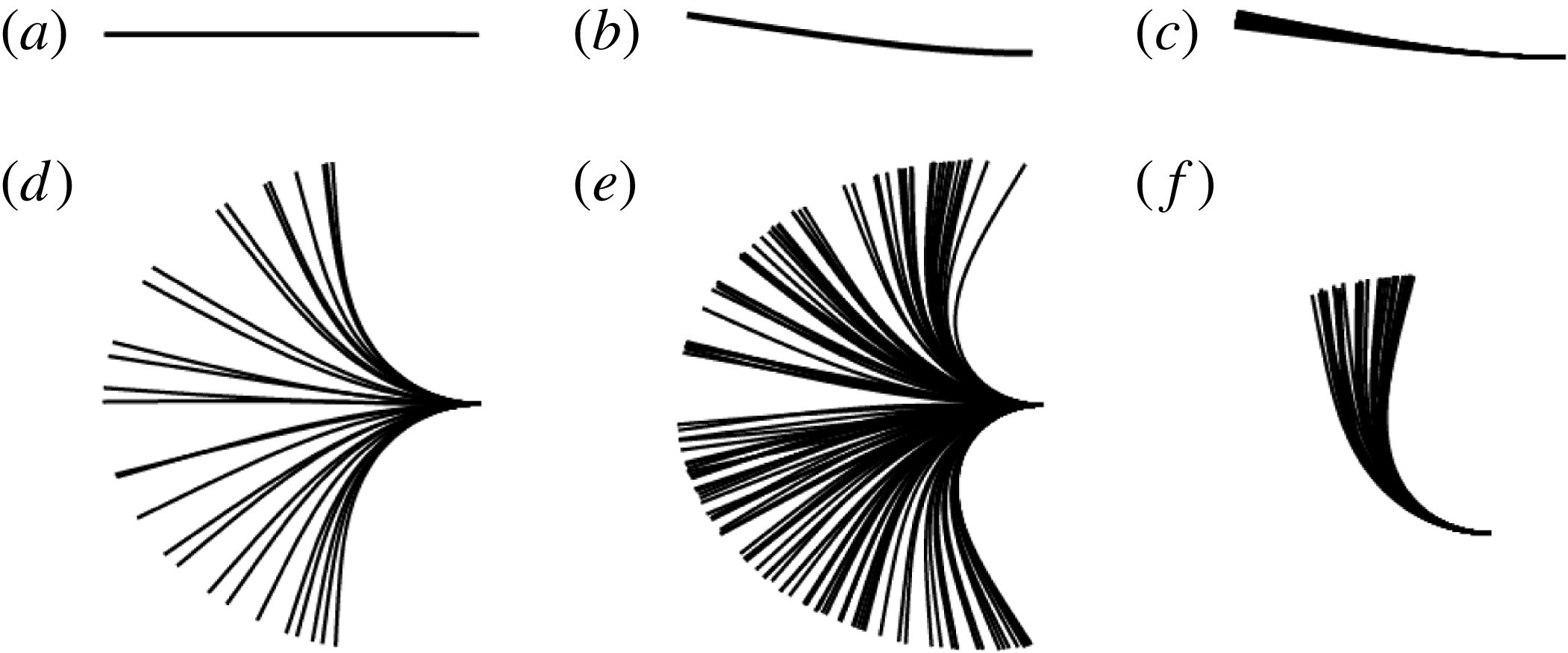
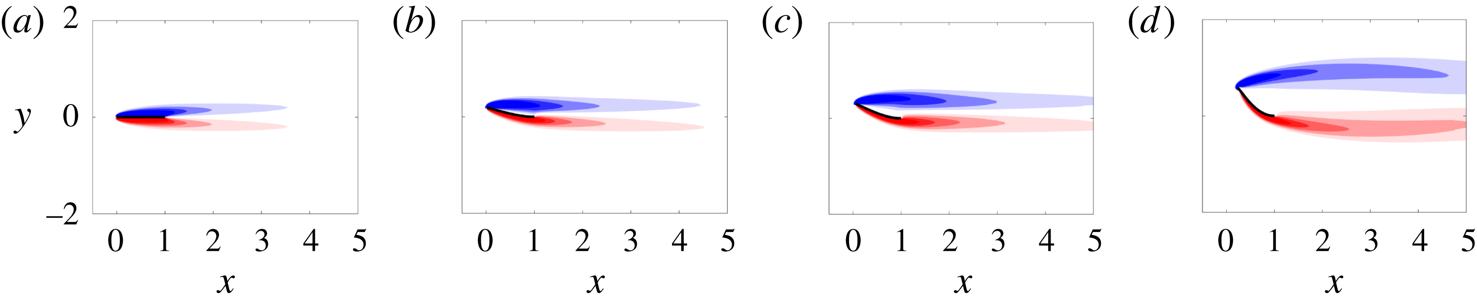
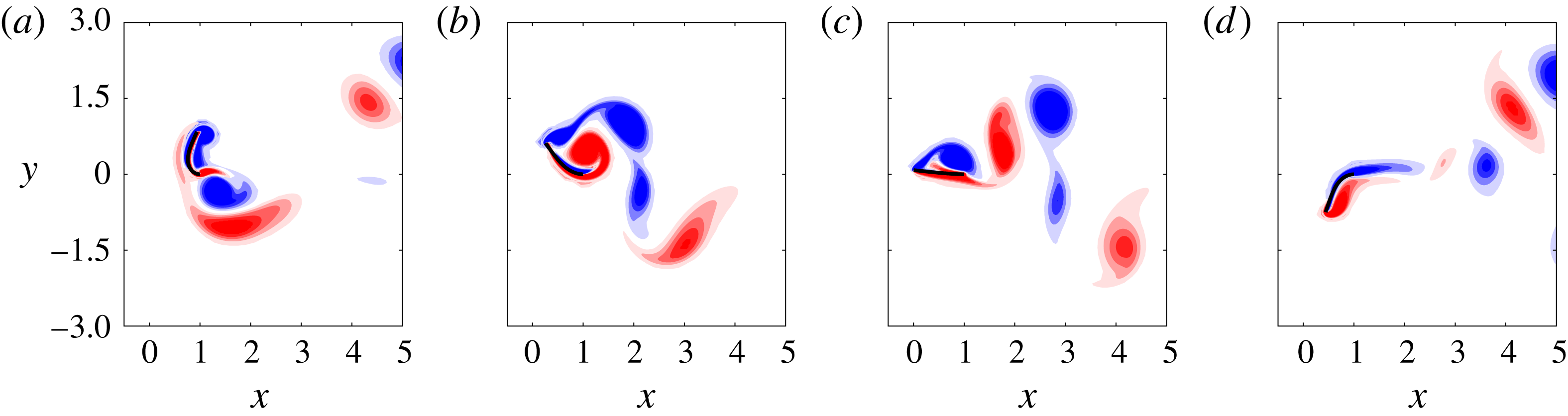
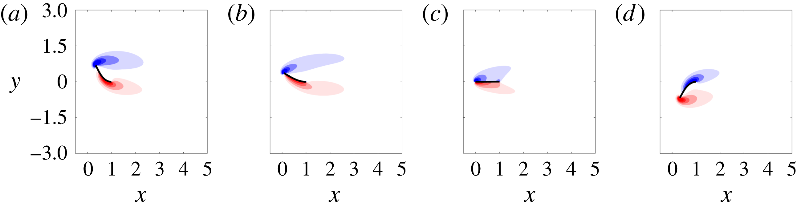
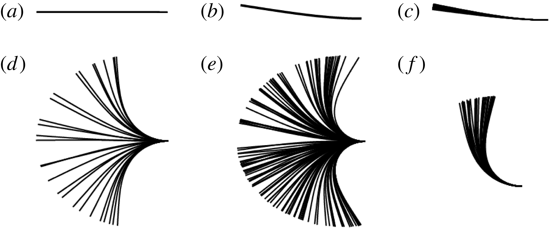
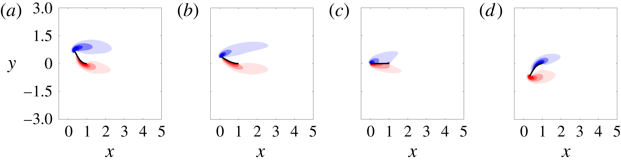
Uniform flow past a conventional flag – where the flag is pinned or clamped at its leading edge with respect to the oncoming flow – has been studied widely beginning with the early work of Taneda (Reference Taneda1968) (see Shelley & Zhang (Reference Shelley and Zhang2011) for a recent review). By contrast, studies of flow past an inverted flag, in which the flag is clamped at its trailing edge, have only been reported recently. The inverted-flag system displays a wide range of dynamical regimes (Kim et al. Reference Kim, Cossé, Cerdeira and Gharib2013; Gurugubelli & Jaiman Reference Gurugubelli and Jaiman2015; Ryu et al. Reference Ryu, Park, Kim and Sung2015), many of which are depicted in figure 1. This figure is produced from the numerical simulations described in § 2.
One of the dynamical regimes depicted is large-amplitude flapping (figure 1 d), which is associated with a larger strain energy than that of conventional flag flapping. These large bending strains make the inverted-flag system a promising candidate for energy harvesting technologies that convert strain energy to electricity, e.g. by using piezoelectric materials. Shoele & Mittal (Reference Shoele and Mittal2016) studied this energy harvesting potential in detail by performing numerical simulations of a fully coupled fluid–structure–piezoelectric model.
Time lapses of flag position for (a) the undeformed equilibrium, (b) small-deflection stable, (c) small-deflection flapping, (d) large-amplitude flapping, (e) chaotic flapping and (f) deflected-mode regimes. In all figures, the flag is clamped at its right edge and the flow direction is from left to right.
Transitions between the various regimes in figure 1 depend on the Reynolds number (
 $Re$
), dimensionless mass ratio (
 $M_{\unicode[STIX]{x1D70C}}$
) and dimensionless bending stiffness (
 $K_{B}$
), defined as
 $$\begin{eqnarray}\displaystyle Re=\frac{\unicode[STIX]{x1D70C}_{f}UL}{\unicode[STIX]{x1D707}},\quad M_{\unicode[STIX]{x1D70C}}=\frac{\unicode[STIX]{x1D70C}_{s}h}{\unicode[STIX]{x1D70C}_{f}L},\quad K_{B}=\frac{D}{\unicode[STIX]{x1D70C}_{f}U^{2}L^{3}}, & & \displaystyle\end{eqnarray}$$
where
 $\unicode[STIX]{x1D70C}_{f}$
(
 $\unicode[STIX]{x1D70C}_{s}$
) is the fluid (structure) density,
 $U$
is the free-stream velocity,
 $L$
is the flag length,
 $\unicode[STIX]{x1D707}$
is the shear viscosity of the fluid,
 $h$
is the flag thickness and
 $D=Eh^{3}/\!(\!12(1-\unicode[STIX]{x1D708}^{2})$
is the flexural rigidity of the flag (where
 $E$
is Young’s modulus of elasticity and
 $\unicode[STIX]{x1D708}$
is Poisson’s ratio). In experiments, regime transitions are triggered by increasing the flow rate (Kim et al.
Reference Kim, Cossé, Cerdeira and Gharib2013). This coincides with a decrease in
 $K_{B}$
and an increase in
 $Re$
for fixed
 $M_{\unicode[STIX]{x1D70C}}$
, by virtue of (1.1). In contrast, numerical simulations often decrease the flag’s stiffness at fixed
 $Re$
and
 $M_{\unicode[STIX]{x1D70C}}$
, which isolates the effect of various parameters and facilitates comparison to previous numerical studies of flow-induced vibration. In the remainder of the article all quantities are dimensionless, with length scales, velocity scales and time scales non-dimensionalised by
 $L$
,
 $U$
and
 $L/U$
, respectively.
Simulations show that for moderate Reynolds numbers (
 ${\lesssim}$
1000), a systematic decrease in
 $K_{B}$
causes a change from a stable undeformed equilibrium state (figure 1
a) to a small-deflection stable state (figure 1
b). This is followed by a transition to small-deflection flapping (figure 1
c), then to large-amplitude flapping (figure 1
d) and finally to a deflected-mode regime (figure 1
f) (Gurugubelli & Jaiman Reference Gurugubelli and Jaiman2015; Ryu et al.
Reference Ryu, Park, Kim and Sung2015). These simulations have been performed primarily for
 $M_{\unicode[STIX]{x1D70C}}\leqslant O(1)$
(heavy fluid loading), although Shoele & Mittal (Reference Shoele and Mittal2016) considered large values of
 $M_{\unicode[STIX]{x1D70C}}$
.
The same regime transitions persist at higher Reynolds numbers,
 $Re\sim O(10^{4})$
, except that the small-deflection stable and small-deflection flapping regimes discussed above have not been observed in measurement. That is, the undeformed equilibrium directly gives way to large-amplitude flapping (Kim et al.
Reference Kim, Cossé, Cerdeira and Gharib2013). Moreover, Sader et al. (Reference Sader, Cossé, Kim, Fan and Gharib2016a
) experimentally identified a chaotic flapping regime (figure 1
e) at these higher Reynolds numbers that has yet to be reported using numerical simulations with
 $Re\leqslant O(1000)$
. Note from figure 1 that chaotic flapping can be difficult to distinguish from large-amplitude flapping from time-lapse images. We will discuss the differences in more detail in subsequent sections.
At low Reynolds numbers (
 $Re\lesssim 50$
), numerical simulations have shown that the inverted flag’s dynamics can change significantly: no flapping occurs, with the only observed regimes being the undeformed equilibrium and stable deflected states (Ryu et al.
Reference Ryu, Park, Kim and Sung2015; Shoele & Mittal Reference Shoele and Mittal2016). These simulations were performed over a wide range of
 $K_{B}$
for only one value of
 $M_{\unicode[STIX]{x1D70C}}$
, and the system’s dependence on these two parameters remains an open question at these lower Reynolds numbers.
Several driving mechanisms of the various regimes illustrated in figure 1(a–f) have been identified. The bifurcation from the undeformed equilibrium is caused by a divergence instability (i.e. a ‘buckling’ instability where the hydrodynamic lift balances the elastic restoring force of the flag – the instability is independent of
 $M_{\unicode[STIX]{x1D70C}}$
). This mechanism was originally suggested by Kim et al. (Reference Kim, Cossé, Cerdeira and Gharib2013), and subsequently found computationally (Gurugubelli & Jaiman Reference Gurugubelli and Jaiman2015) and mathematically via a linear stability analysis (Sader et al.
Reference Sader, Cossé, Kim, Fan and Gharib2016a
).
For large-amplitude flapping, Sader et al. (Reference Sader, Cossé, Kim, Fan and Gharib2016a
) used experiments and a scaling analysis to argue that for a distinct set of parameters this regime is a vortex-induced vibration (VIV); i.e. vortex shedding and flapping occur in synchrony, with flag motion and fluid forces sharing the same dominant frequency (Khalak & Williamson Reference Khalak and Williamson1999; Sarpkaya Reference Sarpkaya2004). This definition of VIV shall henceforth be referred to as ‘classical VIV’ in this article. All other flapping regimes not associated with this frequency synchronisation are characterised as not exhibiting classical VIV. We specify these distinctions for clarity, since there is no single universally agreed-upon definition for VIV. The primary role of vortex shedding in large-amplitude flapping is further evidenced by the above-mentioned observation of Ryu et al. (Reference Ryu, Park, Kim and Sung2015) and Shoele & Mittal (Reference Shoele and Mittal2016) that flapping does not occur below
 $Re\approx 50$
(for certain values of
 $M_{\unicode[STIX]{x1D70C}}$
). Despite these connections, Gurugubelli & Jaiman (Reference Gurugubelli and Jaiman2017) identified distinctions between large-amplitude flapping and classical cylinder VIV by introducing a splitter plate at the trailing edge of the flag. The authors found large-amplitude flapping to persist despite the fact that the splitter plate removed interactions between the counter-rotating vortices. Gurugubelli & Jaiman (Reference Gurugubelli and Jaiman2017) concluded that the leading-edge vortex drives large-amplitude flapping, whereas by contrast counter-rotating vortex interactions are essential for cylinder VIV. These investigations were based on simulations for one value of
 $M_{\unicode[STIX]{x1D70C}}$
, and relationships between vortex dynamics and inverted-flag flapping at other mass ratios remain an open question. Based on a scaling analysis, Sader et al. (Reference Sader, Cossé, Kim, Fan and Gharib2016a
) predicted that classical VIV should cease as the mass ratio,
 $M_{\unicode[STIX]{x1D70C}}$
, increases – a prediction that is yet to be verified. (Note that Sader et al. (Reference Sader, Cossé, Kim, Fan and Gharib2016a
) worked in terms of the reciprocal of the present mass ratio.)
Finally, with respect to the deflected-mode regime, small-amplitude flapping about a large mean-deflected position occurs. Shoele & Mittal (Reference Shoele and Mittal2016) showed that the flapping frequency is identical to that of the vortex shedding caused by the flag’s bluffness.
In this article, we use high-fidelity nonlinear simulations and a global linear stability analysis to further characterise the regimes in figure 1 and explore their driving physical mechanisms. We emphasise that our global stability analysis is based on a linearisation of the fully coupled fluid–structure system of equations. Moreover, the computed equilibria are steady-state solutions of the fully coupled nonlinear equations described in § 2. Our results are presented for Reynolds numbers of 20 and 200, various values of
 $K_{B}$
and values of
 $M_{\unicode[STIX]{x1D70C}}$
spanning four orders of magnitude.
The specific goals of this study are to (i) study the mechanisms responsible for the onset of small-deflection flapping, (ii) probe the role of vorticity generation (including vortex shedding) and VIV in large-amplitude flapping and (iii) investigate whether chaotic flapping occurs at moderate-to-low Reynolds numbers,
 $Re=200$
(§ 3) and
 $Re=20$
(§ 4). Regarding (i), we demonstrate in §§ 3.1 and 4.1 that for both Reynolds numbers (
 $Re=20$
and 200) the small-deflection stable state is an equilibrium of the fully coupled fluid–structure system. The subsequent transition from the deformed equilibrium to small-deflection flapping (figure 1
c), as the bending stiffness decreases, is then shown through a global stability analysis to be a supercritical Hopf bifurcation (§§ 3.2 and 4.2).
For point (ii), we show in § 3.3 that for
 $M_{\unicode[STIX]{x1D70C}}<O(1)$
and
 $Re=200$
, classical VIV can occur in the form of large-amplitude flapping. Classical VIV does not occur for large values of
 $M_{\unicode[STIX]{x1D70C}}$
at
 $Re=200$
(§ 3.3) or for any mass ratio at
 $Re=20$
(§ 4.3), confirming the predictions of Sader et al. (Reference Sader, Cossé, Kim, Fan and Gharib2016a
) based on a scaling analysis. Yet, for both Reynolds numbers, heavy flags (large
 $M_{\unicode[STIX]{x1D70C}}$
) are shown to undergo large-amplitude flapping despite the absence of classical VIV. The mechanisms driving flapping when classical VIV is not present are explored in §§ 3.3 and 4.3.
Finally, with respect to (iii), we confirm in § 3.4 that chaotic flapping occurs at
 $Re=200$
for sufficiently light flags (
 $M_{\unicode[STIX]{x1D70C}}<O(1)$
), and demonstrate that the structure of the associated strange attractor is controlled by a combination of the large-amplitude and deflected-mode regimes. Chaos does not occur for heavy flags (
 $M_{\unicode[STIX]{x1D70C}}>O(1)$
) at
 $Re=200$
or for any mass ratio considered at
 $Re=20$
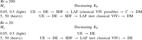
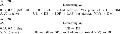
. Thus, chaos is associated with parameters for which classical VIV flapping occurs, and we discuss the relationship between classical VIV and chaos below. Our main conclusions with regard to the regimes of flapping are summarised in table 1.
Overview of regimes obtained by decreasing the stiffness (
 $K_{B}$
) for the mass ratios (
 $M_{\unicode[STIX]{x1D70C}}$
) and Reynolds numbers (
 $Re$
) considered in this article. UE, undeformed equilibrium; DE, deformed equilibrium; SDF, small-deflection flapping; LAF, large-amplitude flapping; C, chaos; DM, deflected mode.
In what follows, we have restricted our analysis to two-dimensional (2-D) flow and flag deformation. As mentioned above, many similarities exist between the 3-D experiments of Kim et al. (Reference Kim, Cossé, Cerdeira and Gharib2013) and 2-D simulations of Gurugubelli & Jaiman (Reference Gurugubelli and Jaiman2015), Ryu et al. (Reference Ryu, Park, Kim and Sung2015) and Shoele & Mittal (Reference Shoele and Mittal2016). This suggests that features of the 2-D dynamics persist in three dimensions, although Sader, Huertas-Cerdeira & Gharib (Reference Sader, Huertas-Cerdeira and Gharib2016b ) demonstrated that substantial differences occur for low aspect ratio flags. Further exploration of three-dimensional effects awaits future studies.
2 Numerical methods: nonlinear solver and global stability analysis
Our nonlinear simulations use the immersed-boundary method of Goza & Colonius (Reference Goza and Colonius2017). The method treats the fluid with the 2-D Navier–Stokes equations, and the 2-D flag with the geometrically nonlinear Euler–Bernoulli beam equation. The method is strongly coupled (i.e. it accounts for the nonlinear coupling between the flag and the fluid), and therefore allows for arbitrarily large flag displacements and rotations. We have validated our method against a variety of test problems involving conventional and inverted flags (Goza & Colonius Reference Goza and Colonius2017). The global stability analysis is based on a linearisation of the nonlinear, fully coupled flow–structure interaction system, and therefore reveals instability-driving mechanisms in both the flag and the fluid.
In what follows, we review the nonlinear solver (see Goza & Colonius (Reference Goza and Colonius2017) for more details) and derive the linearised equations. We then describe the global mode solution approach, the procedure used to compute equilibria of the flow–flag system, and the grid spacing and domain size used for our simulations.
2.1 Nonlinear solver
We define the fluid domain as
 $\unicode[STIX]{x1D6FA}$
and the flag surface as
 $\unicode[STIX]{x1D6E4}$
. We let
 $\boldsymbol{x}$
denote the Eulerian coordinate representing a position in space, and
 $\unicode[STIX]{x1D74C}(\unicode[STIX]{x1D703},t)$
be the Lagrangian coordinate attached to the body
 $\unicode[STIX]{x1D6E4}$
(
 $\unicode[STIX]{x1D703}$
is a variable that parametrises the surface). The dimensionless governing equations are written as
 $$\begin{eqnarray}\displaystyle & \displaystyle \frac{\unicode[STIX]{x2202}\boldsymbol{u}}{\unicode[STIX]{x2202}t}=-\boldsymbol{u}\boldsymbol{\cdot }\unicode[STIX]{x1D735}\boldsymbol{u}-\unicode[STIX]{x1D735}p+\frac{1}{Re}\unicode[STIX]{x1D6FB}^{2}\boldsymbol{u}+\int _{\unicode[STIX]{x1D6E4}}\boldsymbol{f}(\unicode[STIX]{x1D74C}(\unicode[STIX]{x1D703},t))\unicode[STIX]{x1D6FF}(\unicode[STIX]{x1D74C}(\unicode[STIX]{x1D703},t)-\boldsymbol{x})\,\text{d}\unicode[STIX]{x1D703}, & \displaystyle\end{eqnarray}$$
 $$\begin{eqnarray}\displaystyle & \displaystyle \unicode[STIX]{x1D735}\boldsymbol{\cdot }\boldsymbol{u}=0, & \displaystyle\end{eqnarray}$$
 $$\begin{eqnarray}\displaystyle & \displaystyle \frac{\unicode[STIX]{x1D70C}_{s}}{\unicode[STIX]{x1D70C}_{f}}\frac{\unicode[STIX]{x2202}^{2}\unicode[STIX]{x1D74C}}{\unicode[STIX]{x2202}t^{2}}=\frac{1}{\unicode[STIX]{x1D70C}_{f}U^{2}}\unicode[STIX]{x1D735}\boldsymbol{\cdot }\unicode[STIX]{x1D748}+\boldsymbol{g}(\unicode[STIX]{x1D74C})-\boldsymbol{f}(\unicode[STIX]{x1D74C}), & \displaystyle\end{eqnarray}$$
 $$\begin{eqnarray}\displaystyle & \displaystyle \int _{\unicode[STIX]{x1D6FA}}\boldsymbol{u}(\boldsymbol{x})\unicode[STIX]{x1D6FF}(\boldsymbol{x}-\unicode[STIX]{x1D74C}(\unicode[STIX]{x1D703},t))\,\text{d}\boldsymbol{x}=\frac{\unicode[STIX]{x2202}\unicode[STIX]{x1D74C}(\unicode[STIX]{x1D703},t)}{\unicode[STIX]{x2202}t}. & \displaystyle\end{eqnarray}$$
In the above, equation (2.1) expresses the Navier–Stokes equations in an immersed-boundary formulation, equation (2.2) is the continuity equation for the fluid, equation (2.3) represents the structural equations governing the motion of the flag (
 $\boldsymbol{g}$
is a body force term), and (2.4) is the no-slip boundary condition enforcing that the fluid velocity matches the flag velocity on the flag surface. Note that
 $\boldsymbol{f}$
represents the effect from the flag surface stresses on the fluid, and is present in both (2.1) and (2.3) since by Newton’s third law its negative imparts the fluid stresses on the flag surface (Goza & Colonius Reference Goza and Colonius2017). In (2.3), the time derivative is a Lagrangian derivative and the stress tensor is the Cauchy tensor in terms of the deformed flag configuration.
The fluid equations are spatially discretised with the immersed-boundary discrete-streamfunction formulation of Colonius & Taira (Reference Colonius and Taira2008), which removes the pressure and eliminates the continuity equation. The flag equations are treated with a finite-element corotational formulation (Criesfield Reference Criesfield1991). The spatially discrete, temporally continuous equations written as a first-order system of differential–algebraic equations are
 $$\begin{eqnarray}\displaystyle & \displaystyle \unicode[STIX]{x1D63E}^{\text{T}}\unicode[STIX]{x1D63E}\dot{\boldsymbol{s}}=-\unicode[STIX]{x1D63E}^{\text{T}}\boldsymbol{{\mathcal{N}}}(\boldsymbol{s})+\frac{1}{Re}\unicode[STIX]{x1D63E}^{\text{T}}\unicode[STIX]{x1D647}\unicode[STIX]{x1D63E}\boldsymbol{s}-\unicode[STIX]{x1D63E}^{\text{T}}\unicode[STIX]{x1D640}^{\text{T}}(\unicode[STIX]{x1D74C})\boldsymbol{f}, & \displaystyle\end{eqnarray}$$
 $$\begin{eqnarray}\displaystyle & \displaystyle \unicode[STIX]{x1D648}\dot{\unicode[STIX]{x1D73B}}=-\boldsymbol{R}(\unicode[STIX]{x1D74C})+\unicode[STIX]{x1D64C}(\boldsymbol{g}+\unicode[STIX]{x1D652}(\unicode[STIX]{x1D74C})\boldsymbol{f}), & \displaystyle\end{eqnarray}$$
 $$\begin{eqnarray}\displaystyle & \displaystyle \dot{\unicode[STIX]{x1D74C}}=\unicode[STIX]{x1D73B}, & \displaystyle\end{eqnarray}$$
 $$\begin{eqnarray}\displaystyle & \displaystyle \mathbf{0}=\unicode[STIX]{x1D640}(\unicode[STIX]{x1D74C})\unicode[STIX]{x1D63E}\boldsymbol{s}-\unicode[STIX]{x1D73B}, & \displaystyle\end{eqnarray}$$
where
 $\unicode[STIX]{x1D74C}$
and
 $\boldsymbol{f}$
are discrete analogues to their continuous counterparts,
 $\boldsymbol{s}$
is the discrete streamfunction,
 $\unicode[STIX]{x1D73B}$
is the flag velocity and all other variables are defined below.
Equation (2.5) represents the Navier–Stokes equations written in a discrete-streamfunction formulation, equation (2.6) is the geometrically nonlinear Euler–Bernoulli beam equation, equation (2.7) matches the time derivative of the flag position to the flag velocity and (2.8) is the interface constraint that the fluid and flag must satisfy the no-slip boundary condition on the flag surface.
In (2.5)–(2.8),
 $\unicode[STIX]{x1D63E}$
and
 $\unicode[STIX]{x1D63E}^{\text{T}}$
are discrete curl operators that mimic
 $\unicode[STIX]{x1D735}\times (\cdot )$
;
 $\boldsymbol{{\mathcal{N}}}(\boldsymbol{s})$
is a discretisation of the advection operator
 $\boldsymbol{u}\boldsymbol{\cdot }\unicode[STIX]{x1D735}\boldsymbol{u}$
written in terms of the discrete streamfunction (Colonius & Taira Reference Colonius and Taira2008);
 $\unicode[STIX]{x1D647}$
is a discrete Laplacian associated with the viscous diffusion term;
 $\unicode[STIX]{x1D640}^{\text{T}}\boldsymbol{f}$
is a ‘smearing’ operator (arising from the immersed-boundary treatment) that applies the surface stresses from the flag onto the fluid;
 $\unicode[STIX]{x1D648}$
is a mass matrix associated with the flag’s inertia;
 $\boldsymbol{R}(\unicode[STIX]{x1D74C})$
is the internal stress within the flag;
 $\unicode[STIX]{x1D64C}\boldsymbol{g}$
is a body force term (e.g. gravity); and
 $\unicode[STIX]{x1D64C}\unicode[STIX]{x1D652}\boldsymbol{f}$
is the stress imposed on the flag from the fluid.
Equation (2.5) is discretised in time using an Adams–Bashforth AB2 scheme for the convective term and a second-order Crank–Nicolson scheme for the diffusive term. The flag equations (2.6)–(2.7) are discretised using an implicit Newmark scheme. The method is strongly coupled, so the constraint equation (2.8) is exactly enforced at each time step including the present one.
A novel feature of our method is the efficient iterative procedure used to treat the nonlinear coupling between the flag and fluid. Many methods use a block-Gauss–Seidel iterative procedure, which converges slowly (or not at all) for light structures (Tian et al. Reference Tian, Dai, Luo, Doyle and Rousseau2014). Other methods use a Newton–Raphson scheme, which exhibits fast convergence behaviour but requires the solution of linear systems involving large Jacobian matrices (Degroote, Bathe & Vierendeels Reference Degroote, Bathe and Vierendeels2009). Our method employs the latter approach, but we use a block-LU factorisation of the Jacobian matrix to restrict all iterations to subsystems whose dimensions scale with the number of discretisation points on the flag, rather than on the entire flow domain. Thus, our algorithm inherits the fast convergence behaviour of Newton–Raphson methods while substantially reducing the cost of performing an iteration.
2.2 Linearised equations and global modes
For ease of notation, we define the state vector
 $\boldsymbol{y}=[\boldsymbol{s},\unicode[STIX]{x1D73B},\unicode[STIX]{x1D74C},\boldsymbol{f}]^{\text{T}}$
and let
 $\boldsymbol{r}(\boldsymbol{y})$
be the right-hand side of (2.5)–(2.8). We write the state as
 $\boldsymbol{y}=\boldsymbol{y}_{b}+\boldsymbol{y}_{p}$
, where
 $\boldsymbol{y}_{b}=[\boldsymbol{s}_{b},\unicode[STIX]{x1D73B}_{b},\unicode[STIX]{x1D74C}_{b},\boldsymbol{f}_{b}]^{\text{T}}$
is a base state and
 $\boldsymbol{y}_{p}=[\boldsymbol{s}_{p},\unicode[STIX]{x1D73B}_{p},\unicode[STIX]{x1D74C}_{p},\boldsymbol{f}_{p}]^{\text{T}}$
is a perturbation. Plugging this expression for
 $\boldsymbol{y}$
into (2.5)–(2.8), Taylor-expanding about
 $\boldsymbol{y}_{b}$
and retaining only first-order terms in the perturbation variables gives the linearised equations
 $$\begin{eqnarray}\displaystyle \unicode[STIX]{x1D63D}\dot{\boldsymbol{y}}_{p}=\unicode[STIX]{x1D63C}(\boldsymbol{y}_{b})\boldsymbol{y}_{p}, & & \displaystyle\end{eqnarray}$$
where
 $$\begin{eqnarray}\displaystyle \unicode[STIX]{x1D63D}=\left[\begin{array}{@{}ccccc@{}}\unicode[STIX]{x1D63E}^{\text{T}}\unicode[STIX]{x1D63E} & & & \\ & \unicode[STIX]{x1D648} & & \\ & & \unicode[STIX]{x1D644} & \\ & & & & \mathbf{0}\end{array}\right],\quad \unicode[STIX]{x1D63C}(\,\boldsymbol{y}_{b})=\left[\begin{array}{@{}cccc@{}}\unicode[STIX]{x1D645}^{ss} & \mathbf{0} & -\unicode[STIX]{x1D645}^{\unicode[STIX]{x1D712}s} & -\unicode[STIX]{x1D63E}^{\text{T}}\unicode[STIX]{x1D640}^{\text{T}}\\ \boldsymbol{ 0} & \mathbf{0} & -\unicode[STIX]{x1D646}+\unicode[STIX]{x1D645}^{\unicode[STIX]{x1D712}\unicode[STIX]{x1D712}} & \unicode[STIX]{x1D64C}\unicode[STIX]{x1D652}\\ \boldsymbol{ 0} & \unicode[STIX]{x1D644} & \mathbf{0} & \mathbf{0}\\ \unicode[STIX]{x1D640}\unicode[STIX]{x1D63E} & -\unicode[STIX]{x1D644} & \unicode[STIX]{x1D645}^{\unicode[STIX]{x1D712}c} & \mathbf{0}\end{array}\right]_{\boldsymbol{y}=\boldsymbol{y}_{b}} & & \displaystyle\end{eqnarray}$$
and the remaining sub-blocks of the Jacobian matrix
 $\unicode[STIX]{x1D63C}$
are given in index notation as
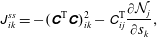 $$\begin{eqnarray}\displaystyle & \displaystyle \unicode[STIX]{x1D611}_{ik}^{ss}=-(\unicode[STIX]{x1D63E}^{\text{T}}\unicode[STIX]{x1D63E})_{ik}^{2}-\unicode[STIX]{x1D60A}_{ij}^{\text{T}}\frac{\unicode[STIX]{x2202}{\mathcal{N}}_{j}}{\unicode[STIX]{x2202}s_{k}}, & \displaystyle\end{eqnarray}$$
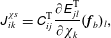 $$\begin{eqnarray}\displaystyle & \displaystyle \unicode[STIX]{x1D611}_{ik}^{\unicode[STIX]{x1D712}s}=\unicode[STIX]{x1D60A}_{ij}^{\text{T}}\frac{\unicode[STIX]{x2202}\unicode[STIX]{x1D60C}_{jl}^{\text{T}}}{\unicode[STIX]{x2202}\unicode[STIX]{x1D712}_{k}}(\boldsymbol{f}_{b})_{l}, & \displaystyle\end{eqnarray}$$
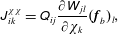 $$\begin{eqnarray}\displaystyle & \displaystyle \unicode[STIX]{x1D611}_{ik}^{\unicode[STIX]{x1D712}\unicode[STIX]{x1D712}}=\unicode[STIX]{x1D618}_{ij}\frac{\unicode[STIX]{x2202}\unicode[STIX]{x1D61E}_{jl}}{\unicode[STIX]{x2202}\unicode[STIX]{x1D712}_{k}}(\boldsymbol{f}_{b})_{l}, & \displaystyle\end{eqnarray}$$
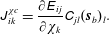 $$\begin{eqnarray}\displaystyle & \displaystyle \unicode[STIX]{x1D611}_{ik}^{\unicode[STIX]{x1D712}c}=\frac{\unicode[STIX]{x2202}\unicode[STIX]{x1D60C}_{ij}}{\unicode[STIX]{x2202}\unicode[STIX]{x1D712}_{k}}\unicode[STIX]{x1D60A}_{jl}(\boldsymbol{s}_{b})_{l}. & \displaystyle\end{eqnarray}$$
Note that we used
 $\unicode[STIX]{x1D63D}\dot{\boldsymbol{y}}_{b}=\boldsymbol{r}(\boldsymbol{y}_{b})$
in arriving at the linearised equations (2.9).
Global modes are eigenvectors
 $\boldsymbol{v}$
of the generalised eigenvalue problem
 $\unicode[STIX]{x1D63C}\boldsymbol{v}=\unicode[STIX]{x1D706}\unicode[STIX]{x1D63D}\boldsymbol{v}$
, where
 $\unicode[STIX]{x1D706}$
is the corresponding eigenvalue. We build and store
 $\unicode[STIX]{x1D63C}$
and
 $\unicode[STIX]{x1D63D}$
sparsely and solve the generalised eigenvalue problem using an implicitly restarted Arnoldi algorithm (see Lehoucq, Sorensen & Yang (Reference Lehoucq, Sorensen and Yang1998) for more details). More details for how the eigenvalue problem is constructed and solved are provided in appendix A.
In the results below,
 $1\times 10^{-10}$
was used as the tolerance for convergence of the computed eigenvalues and eigenvectors. Global eigenfunctions are unique to a scalar multiple, and were scaled to unit norm,
 $\Vert \boldsymbol{y}\Vert _{2}=1$
.
2.3 Equilibrium computations
Undeformed and deformed equilibria are steady-state solutions to the fully coupled equations (2.5)–(2.8) with all time derivate terms set to zero; i.e. these equilibria satisfy
 $\mathbf{0}=\boldsymbol{r}(\boldsymbol{y})$
, where
 $\boldsymbol{y}=[\boldsymbol{s},\unicode[STIX]{x1D73B},\unicode[STIX]{x1D74C},\boldsymbol{f}]^{\text{T}}$
is the state vector and
 $\boldsymbol{r}(\boldsymbol{y})$
is the right-hand side of (2.5)–(2.8). This is a nonlinear algebraic system of equations that we solve using a Newton–Raphson method. With this method, the
 $k$
th guess for the base state,
 $\boldsymbol{y}^{(k)}$
, is updated as
 $\boldsymbol{y}^{(k+1)}=\boldsymbol{y}^{(k)}+\unicode[STIX]{x0394}\boldsymbol{y}$
, where
 $$\begin{eqnarray}\displaystyle \unicode[STIX]{x0394}\boldsymbol{y}=-(\unicode[STIX]{x1D63C}(\boldsymbol{y}^{(k)}))^{-1}\boldsymbol{r}(\boldsymbol{y}^{(k)}). & & \displaystyle\end{eqnarray}$$
Note that the Jacobian matrix
 $\unicode[STIX]{x1D63C}$
in (2.15) is the same matrix as in (2.10) evaluated at
 $\boldsymbol{y}=\boldsymbol{y}^{(k)}$
.
The guess for the state
 $\boldsymbol{y}$
is updated until the residual at the current guess is less than a desired threshold (i.e. until
 $\Vert \boldsymbol{r}(\boldsymbol{y}^{(k)})\Vert _{2}/\Vert \boldsymbol{y}^{(k)}\Vert _{2}<\unicode[STIX]{x1D716}$
). In the results shown below we used
 $\unicode[STIX]{x1D716}=1\times 10^{-6}$
.
2.4 Domain size and grid resolution
The flow equations are treated using a multidomain approach: the finest grid surrounds the body and grids of increasing coarseness are used at progressively larger distances (Colonius & Taira Reference Colonius and Taira2008). In all computations below, the domain size of the finest sub-domain is
 $[-0.2,1.8]\times [-1.1,1.1]$
and the total domain size is
 $[-15.04,16.64]\times [-17.44,17.44]$
. The grid spacing on the finest domain is
 $h=0.01$
and the grid spacing for the flag is
 $\unicode[STIX]{x0394}s=0.02$
. For computations involving time marching, the time step is
 $\unicode[STIX]{x0394}t=0.001$
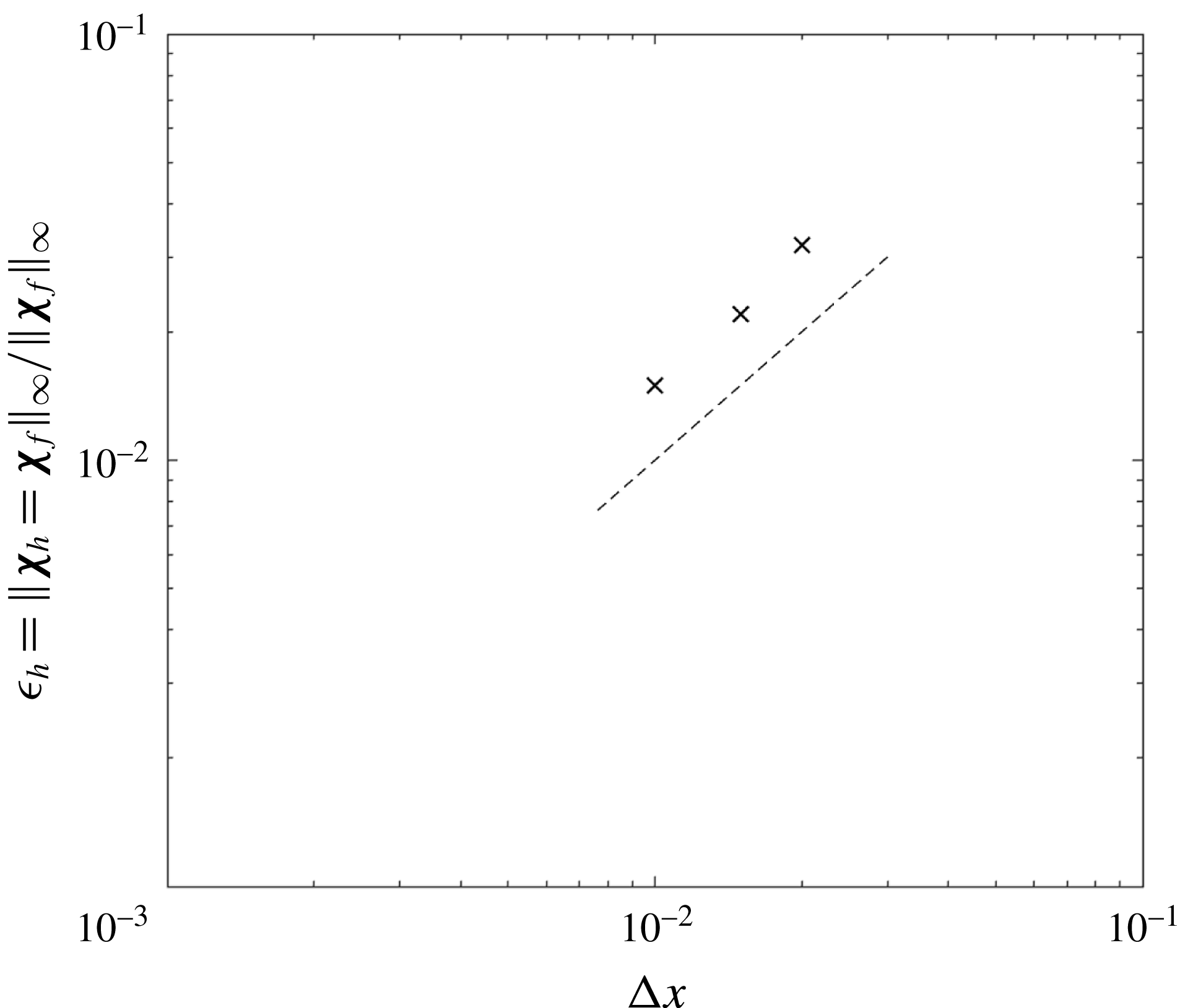
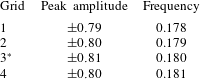
, which gives a maximum Courant–Friedrichs–Lewy number of approximately 0.15. Appendix B contains a convergence study that demonstrates the suitability of these parameters.
3 Dynamics for
 $Re=200$

3.1 Bifurcation diagrams and general observations
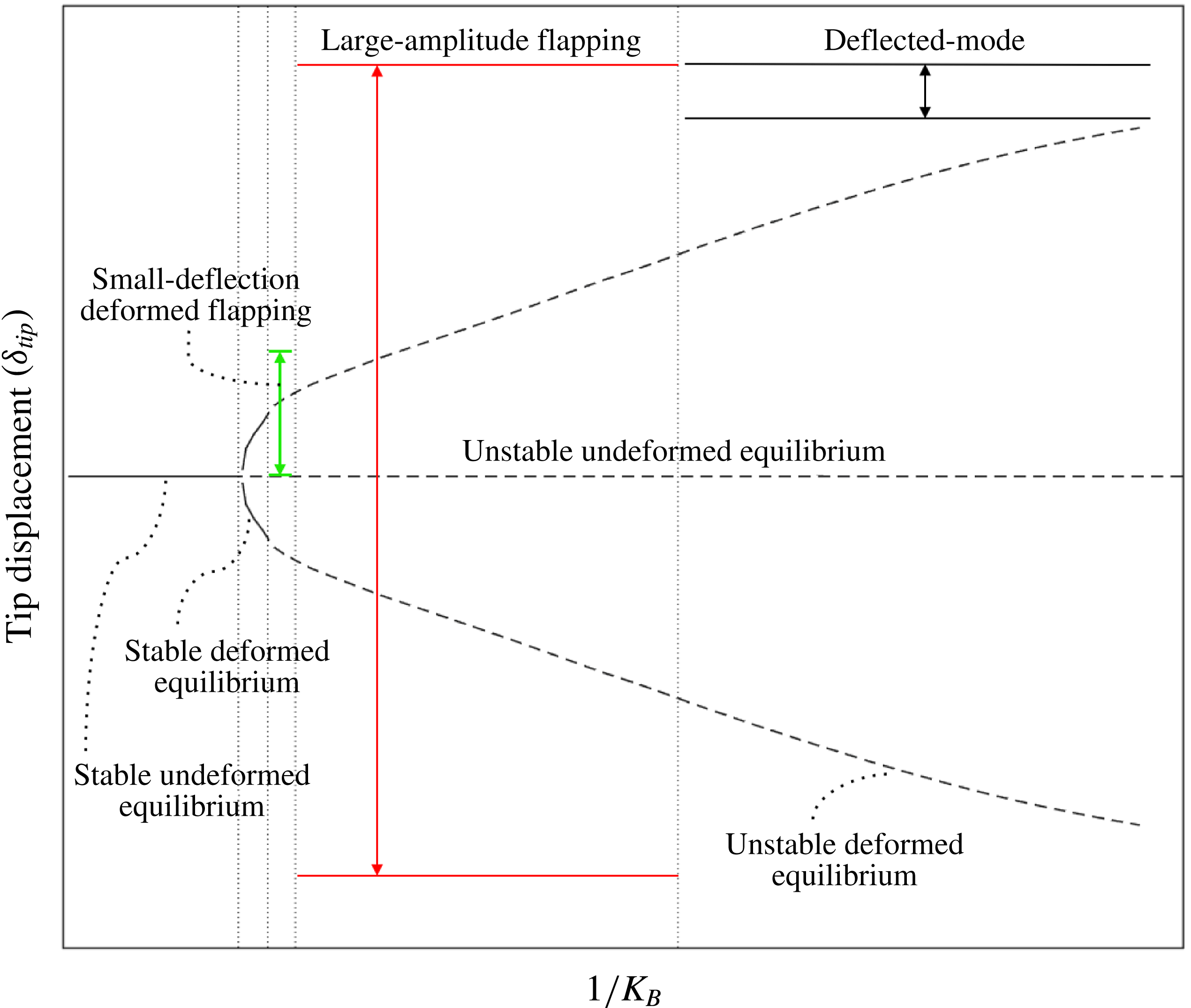
This section contains an overview of the various regimes that are studied in detail in §§ 3.2–3.5. As part of this overview, we use bifurcation diagrams that illustrate the equilibria (and their stability) along with the flapping dynamics. We give a generic version of these bifurcation diagrams in figure 2 that summarises the upcoming diagrams. The leading-edge transverse displacement (tip deflection,
 $\unicode[STIX]{x1D6FF}_{tip}$
) is plotted versus the flag flexibility (
 $1/K_{B}$
) for a particular choice of
 $Re$
and
 $M_{\unicode[STIX]{x1D70C}}$
. The generic diagram in figure 2 demonstrates that with decreasing
 $K_{B}$
(moving left to right on the diagram), the system transitions from the undeformed equilibrium to a stable deformed equilibrium. Following this, the system bifurcates to small-deflection flapping, then large-amplitude flapping (chaotic flapping can also occur in this regime depending on
 $M_{\unicode[STIX]{x1D70C}}$
), and finally to the deflected-mode regime.
A schematic bifurcation diagram that summarises the results obtained for the various parameters considered in this study. Equilibria are presented by lines (——, stable equilibria; – –, unstable equilibria). The lines with the double arrows indicate regimes where flapping occurs, with the top and bottom lines representing the peak-to-peak flapping amplitude.
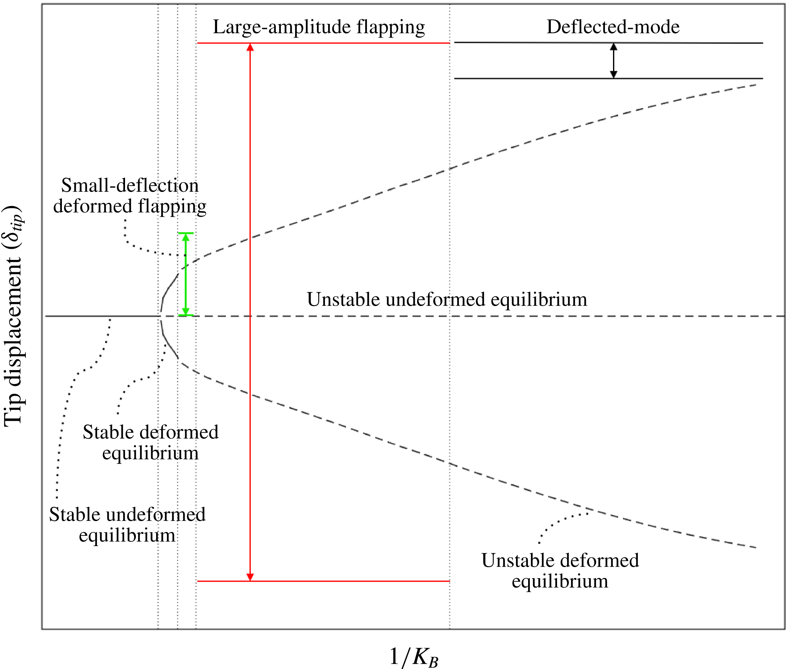
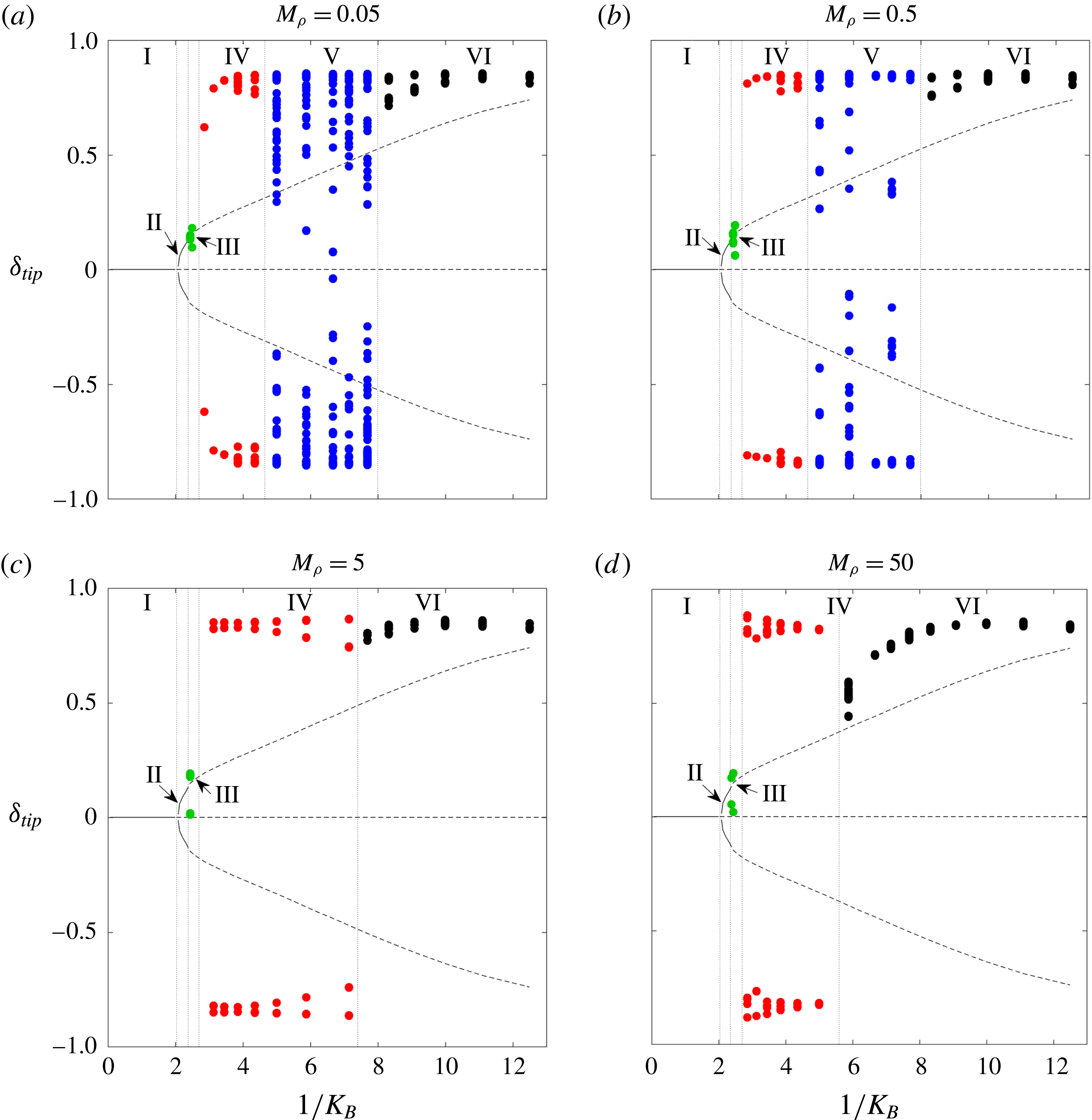
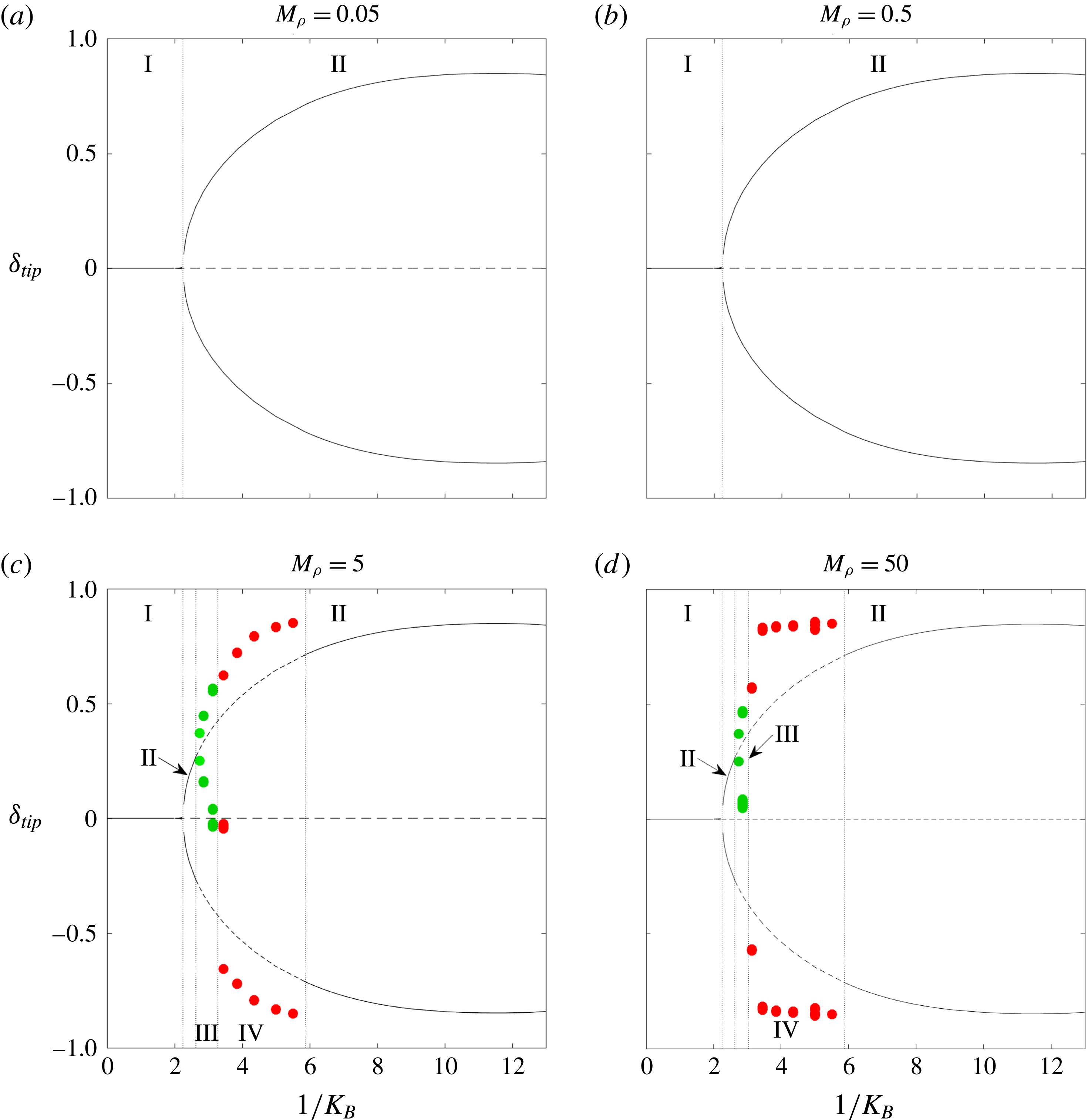
Figure 3 shows bifurcation diagrams at four different mass ratios,
 $M_{\unicode[STIX]{x1D70C}}$
, for
 $Re=200$
. Each plot gives the transverse leading-edge displacement (tip deflection,
 $\unicode[STIX]{x1D6FF}_{tip}$
, non-dimensionalised by the flag length
 $L$
) as a function of the reciprocal dimensionless stiffness (
 $1/K_{B}$
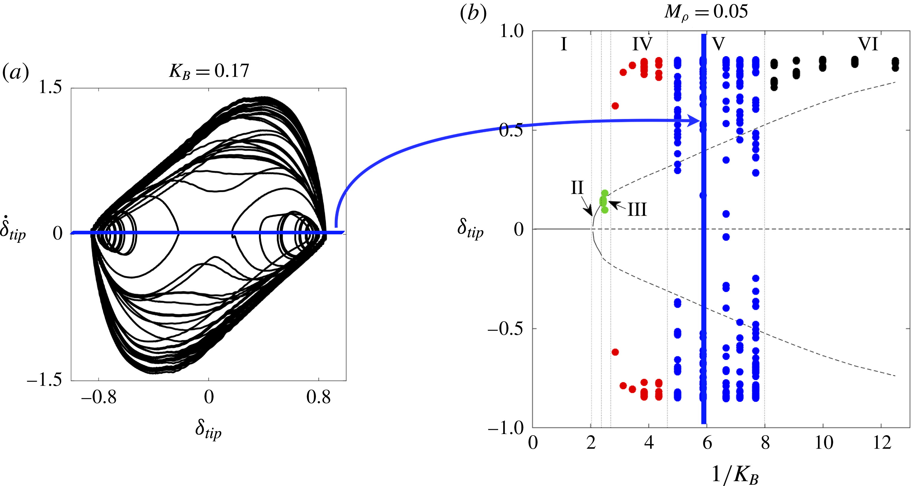
). Solid lines represent stable equilibria, and dashed lines correspond to unstable equilibria. Information for unsteady regimes is conveyed through the markers. A set of markers at a given stiffness corresponds to tip deflection values from a single nonlinear simulation at moments when the tip velocity is zero (i.e. when the flag changes direction at the tip). From a dynamical systems perspective, the markers correspond to zero-tip-velocity Poincaré sections of a velocity-displacement phase portrait of the leading edge. For clarity, appendix C provides further explanation of how the set of markers was obtained at
 $1/K_{B}\approx 6$
for the
 $M_{\unicode[STIX]{x1D70C}}=0.05$
bifurcation diagram.
All nonlinear simulations were started with the flag in its undeflected position and the flow impulsively started at its free-stream value. A small body force was introduced at an early time to trigger any instabilities in the system. All simulations contain a minimum of 15 flapping cycles except for the chaotic flapping regime, where a minimum of 55 cycles were used. To avoid representing transient behaviour in the figures, we omit the first several flapping cycles in the diagrams.
To illustrate the meaning of the markers in figure 3 further, consider
 $1/K_{B}\approx 4$
for
 $M_{\unicode[STIX]{x1D70C}}=0.5$
. The system enters into large-amplitude limit-cycle flapping with a fixed amplitude of
 ${\approx}\pm 0.8$
, and the bifurcation diagram reflects this with a marker at these peak tip displacements, which are the only tip displacement values where the tip velocity is zero. Note that there are actually several markers superimposed onto one another at this stiffness since multiple flapping periods were used to plot these diagrams, though only one marker is visible because of the limit-cycle behaviour exhibited. As another example, the bifurcation diagram at
 $1/K_{B}\approx 6$
for
 $M_{\unicode[STIX]{x1D70C}}=0.05$
depicts chaotic flapping. Many markers are visible at this stiffness because the flag changes direction at several different values of
 $\unicode[STIX]{x1D6FF}_{tip}$
. The merit of using zero-tip-velocity Poincaré sections for the bifurcation diagrams is seen through chaotic flapping: these Poincaré sections demonstrate the variety of transverse locations where the flag changes direction – a fact not captured through, for example, plotting the peak-to-peak flapping amplitudes at a given stiffness.
Bifurcation diagrams of inverted-flag dynamics at
 $Re=200$
that show leading-edge transverse displacement (tip deflection,
 $\unicode[STIX]{x1D6FF}_{tip}$
) versus inverse stiffness (
 $1/K_{B}$
). I, undeformed equilibrium; II, deformed equilibrium; III, small-deflection flapping; IV, large-amplitude flapping; V, chaotic flapping; VI, deflected mode. See the main text for a description of the various lines and markers and details on how the diagrams were constructed.
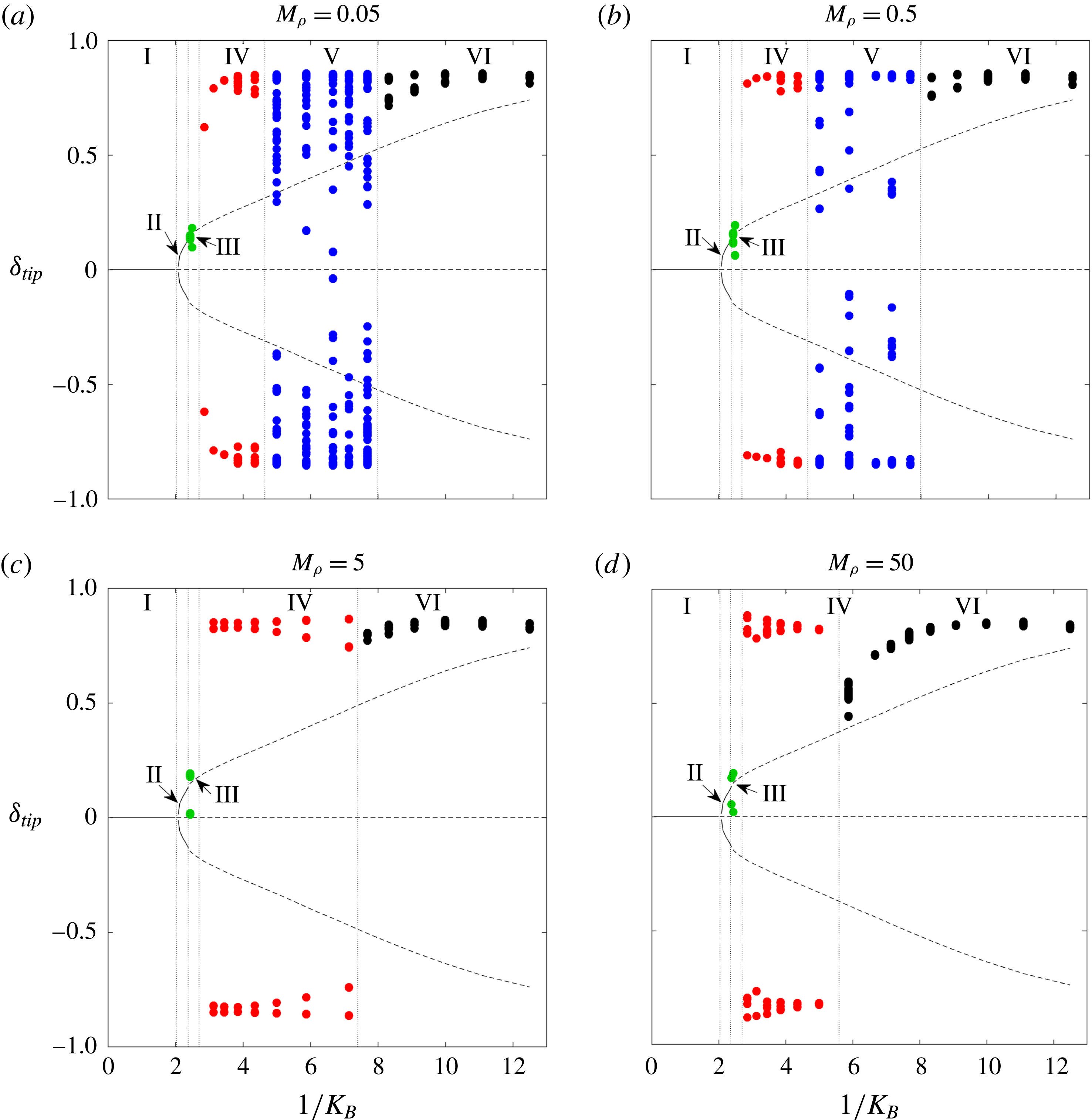
The bifurcation diagrams in figure 3 depict the undeformed equilibrium (I), deformed equilibrium (II), small-deflection flapping (III), large-amplitude flapping (IV), deflected mode (VI) and chaotic flapping (V) regimes. In small-deflection flapping, the flag moves about the upward deflected equilibrium. There is a corresponding deformed equilibrium with a negative flag deflection, and different initial conditions would result in flapping about this equilibrium. We refrain from plotting this behaviour to avoid confusion with large-amplitude flapping. Note that many of these regimes exhibit hysteresis. For example, Kim et al. (Reference Kim, Cossé, Cerdeira and Gharib2013) demonstrated that large-amplitude flapping can be extended to higher stiffnesses by decreasing
 $K_{B}$
while the system is in large-amplitude flapping. We do not investigate this behaviour in the present work.
We now explore the change in behaviour as the flag stiffness,
 $K_{B}$
, is reduced. The undeformed equilibrium becomes unstable with decreasing stiffness due to a divergence instability, i.e. flag buckling, with the critical stiffness for this instability being independent of the mass ratio (Kim et al.
Reference Kim, Cossé, Cerdeira and Gharib2013; Gurugubelli & Jaiman Reference Gurugubelli and Jaiman2015; Sader et al.
Reference Sader, Cossé, Kim, Fan and Gharib2016a
).
We see from figure 3 that following this instability the flag transitions to a steady deflected position (regime II). This deflected steady-state regime was first observed by Ryu et al. (Reference Ryu, Park, Kim and Sung2015), Gurugubelli & Jaiman (Reference Gurugubelli and Jaiman2015), and we note here that it represents a deformed-equilibrium state; i.e. in the notation of § 2 it satisfies the steady-state equations
 $\boldsymbol{r}(\boldsymbol{y})=0$
. (Because the deformed equilibrium is a steady-state solution, it does not depend on flag inertia, and thus its associated tip deflection at a given stiffness does not depend on the mass ratio,
 $M_{\unicode[STIX]{x1D70C}}$
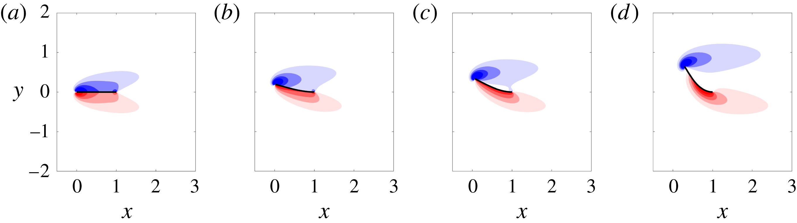
.) With decreasing stiffness, the deformed equilibrium is associated with an increasingly large tip deflection, and transitions from stable (regime II) to unstable (regimes III–VI). When the deformed equilibrium state is unstable, flapping occurs. Figure 4 provides illustrations of deformed equilibria (some of which are unstable) for various stiffnesses. Gurugubelli & Jaiman (Reference Gurugubelli and Jaiman2015) identified a deflected equilibrium using a force and moment balance on the flag, with the fluid modelled as an empirical forcing term. Using this model, the deflected equilibrium was not found for regimes II–V, and was instead observed to appear at approximately the same stiffness value for which the deflected-mode state (regime VI) was seen in the nonlinear simulations. The authors concluded from this that the bifurcation to the deflected-mode regime occurs because of the appearance of the deflected equilibrium. By contrast, computing the equilibria from the fully coupled equations (2.5)–(2.8) demonstrates that the deflected equilibrium first appears in regime II as a stable solution following the divergence instability of the undeformed equilibrium (regime I), and persists as an unstable equilibrium through the various flapping regimes – including the deflected-mode state. The existence of an unstable deflected equilibrium is consistent with the experimental observations of Sader et al. (Reference Sader, Cossé, Kim, Fan and Gharib2016a
) at much higher Reynolds numbers, where a deflected equilibrium was found by introducing structural damping to negate the effects of unsteadiness in the flow.
Vorticity contours for equilibrium states of the flow–inverted-flag system at
 $Re=200$
. From (a) to (b),
 $K_{B}=0.5,0.35,0.22,0.11$
. The three rightmost equilibria are unstable for all masses considered. Contours are in 18 increments from
 $-$
5 to 5.
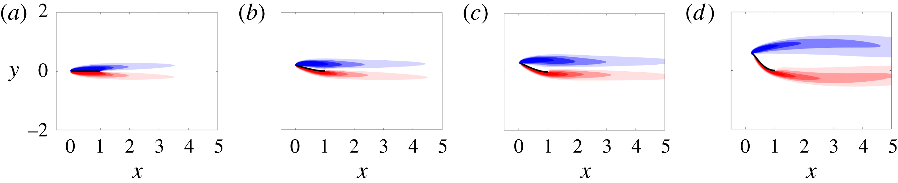
Figure 3 shows that as stiffness is decreased and the deformed equilibrium becomes unstable, flapping ensues. Initially (regime III), this flapping is of small amplitude, with oscillation amplitudes that are smaller than the equilibrium deflection – we refer to this regime as small-deflection flapping. Following small-deflection flapping, light flags (corresponding to small values of
 $M_{\unicode[STIX]{x1D70C}}$
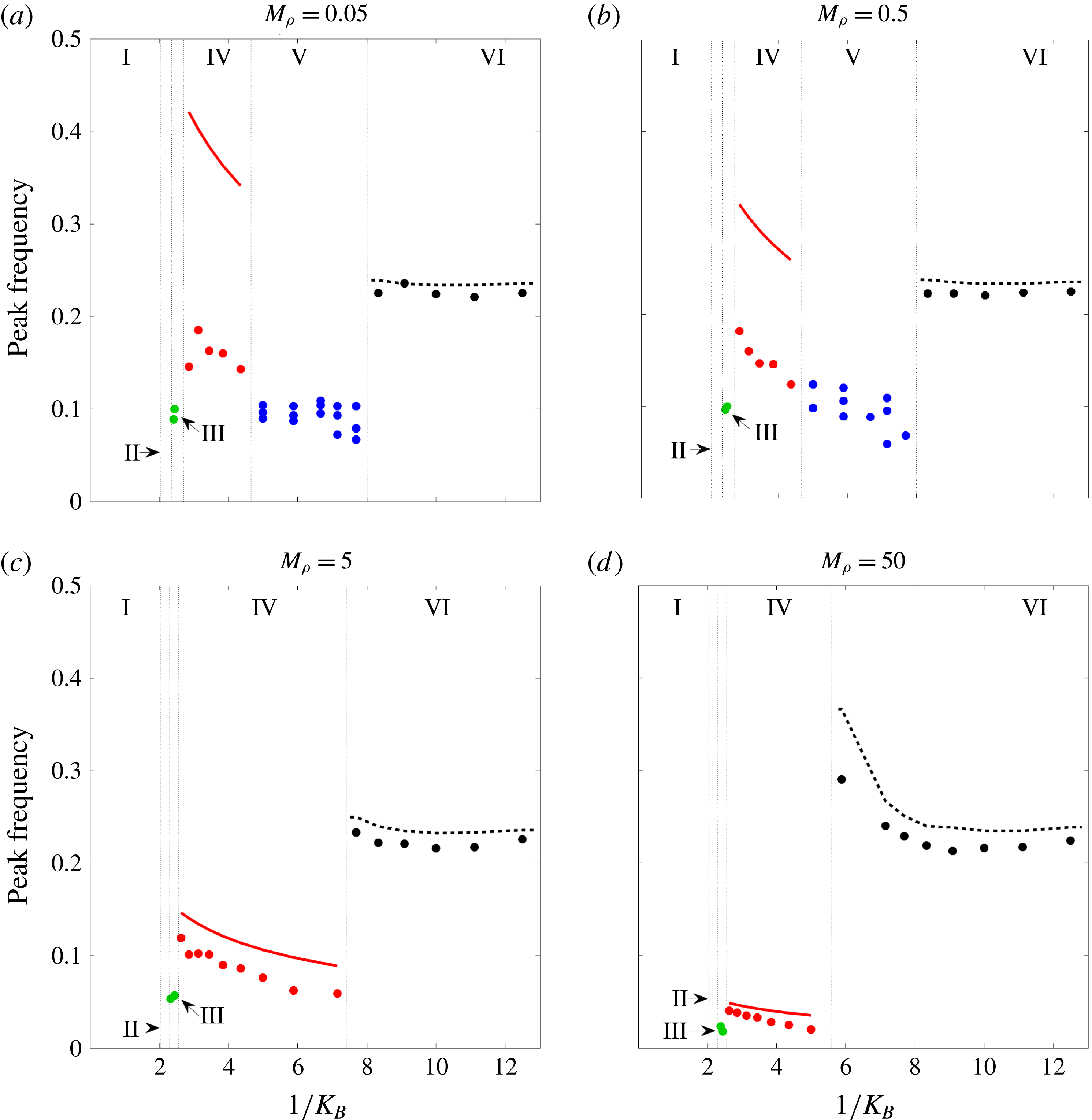
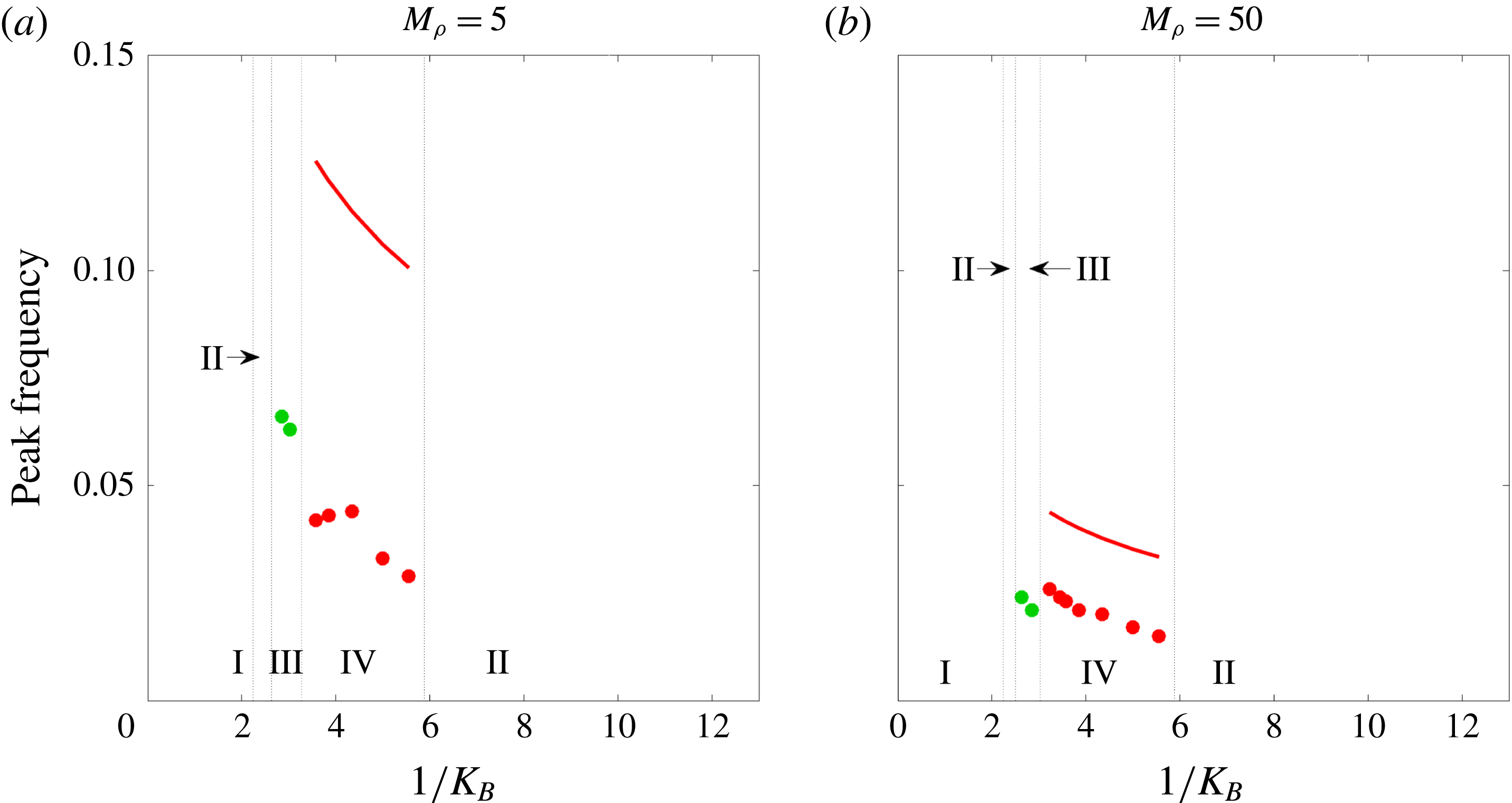
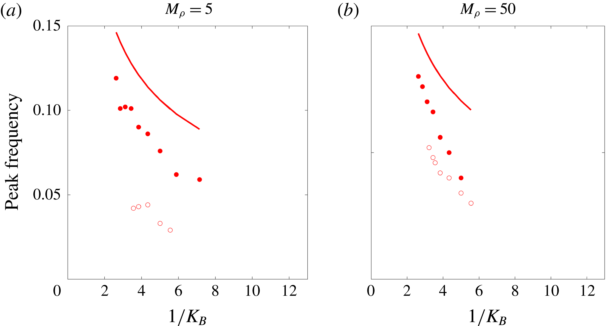
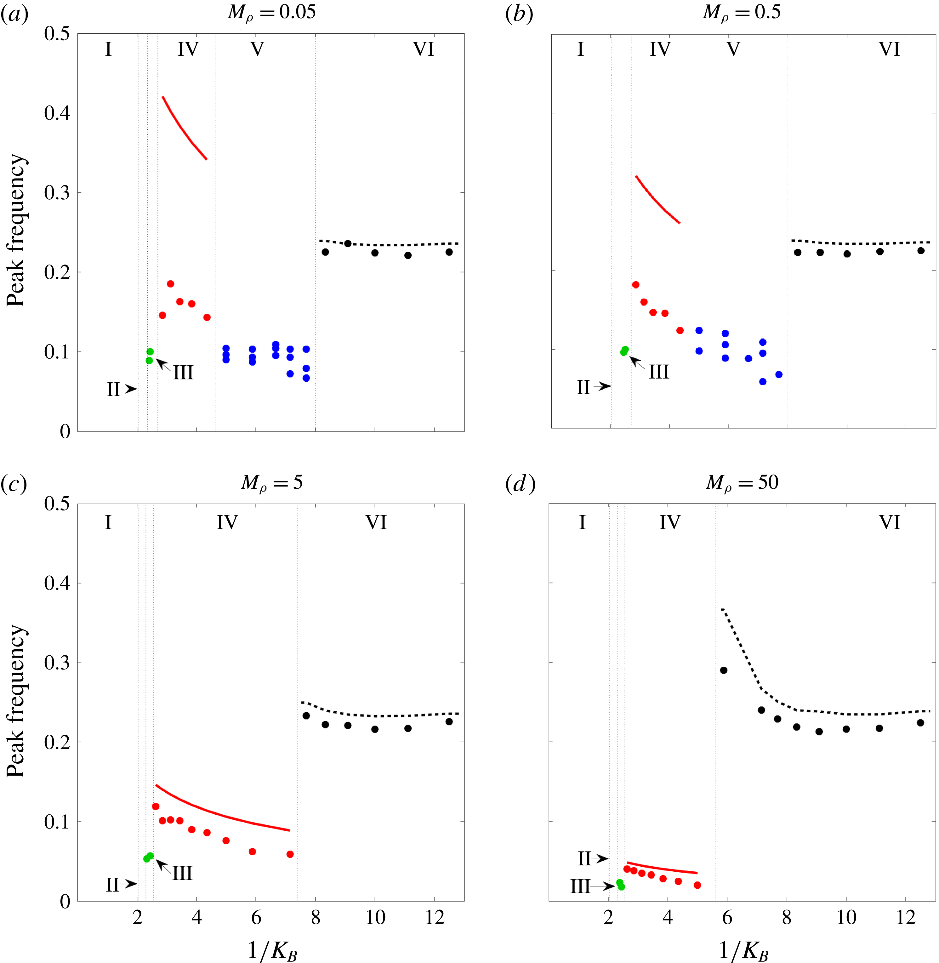
) transition from large-amplitude flapping (regime IV) to chaotic flapping (regime V), and finally the deflected-mode state (regime VI). Heavy flags exhibit the same transitions after small-deflection flapping except that chaos does not occur. The various regimes and their transitions will be explored in further detail in subsequent sections. As context for the subsequent discussions of the flapping regimes, figure 5 gives the peak flapping frequency for the various regimes where flapping occurs (note that chaotic flapping is characterised by a spectrum of frequencies – the figure shows all frequency components containing a minimum of 20 % of the power spectral density). The subsequent sections will refer to the frequency plots in figure 5 (and the bifurcation diagrams in figure 3) where relevant.
Markers: peak flapping frequency at
 $Re=200$
for the parameters corresponding to the bifurcation diagrams shown in figure 3; ——, natural frequency scaling of a sheet accounting for added mass contributions from an inviscid fluid, as derived in Shen, Chakraborty & Sader (Reference Shen, Chakraborty and Sader2016);
– –, bluff-body shedding frequency (
 $=0.2/L_{p}$
, where
 $L_{p}$
is the projected length of the flag to the flow defined using the maximum tip deflection at a given stiffness).
3.2 Small-deflection flapping
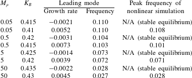
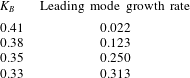
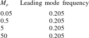
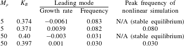
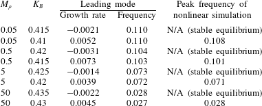
Table 2 demonstrates that the transition to small-deflection flapping occurs via a supercritical Hopf bifurcation of the deformed equilibrium; i.e. for all four mass ratios (
 $M_{\unicode[STIX]{x1D70C}}$
), the onset of flapping is associated with the transition to instability of a complex-conjugate pair of eigenvectors, leading to oscillatory (time-dependent) motion. Table 2 also shows that the leading mode accurately captures the flapping frequency observed in the nonlinear simulations near this stability boundary where flapping amplitudes remain small. Note that for all mass ratios considered, small-deflection flapping is associated with a low dimensionless frequency (Strouhal number) that is not indicative of classical VIV behaviour: using the maximal tip displacement as the normalising length scale, the largest Strouhal number over all masses is 0.02 (
 $\ll 0.2$
, the typical value for classical VIV). The absence of classical VIV is further evidenced by the fact that shedding of distinct vortices, as in the von Kármán vortex street, at each oscillation period of the flag is not evident – Gurugubelli & Jaiman (Reference Gurugubelli and Jaiman2015) demonstrated that the leading-edge vortex formed during small-deflection flapping remains attached throughout the flapping process. This behaviour is also shown in figure 6, which provides snapshots of a flapping period for
 $M_{\unicode[STIX]{x1D70C}}=0.5,K_{B}=0.41$
(i.e. in the small-deflection flapping regime). To explore the mechanism responsible for the onset of small-deflection flapping, we investigate the leading global mode in what follows.
Vorticity contours at four snapshots of a flapping period of a flag in small-deflection flapping. The figures were obtained from a nonlinear simulation with
 $Re=200,M_{\unicode[STIX]{x1D70C}}=0.5,K_{B}=0.41$
. Contours are in 18 increments from
 $-$
5 to 5.

Growth rate and frequency of the leading global mode of the deformed equilibrium compared with nonlinear behaviour for parameters near the onset of small-deflection flapping.
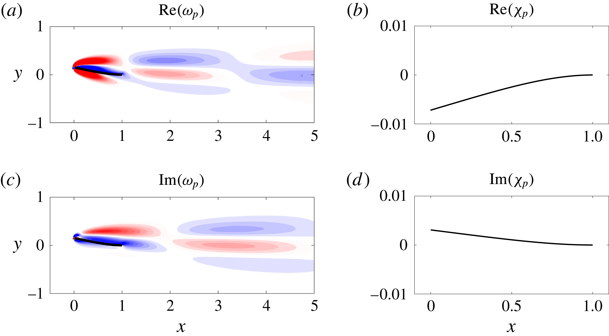
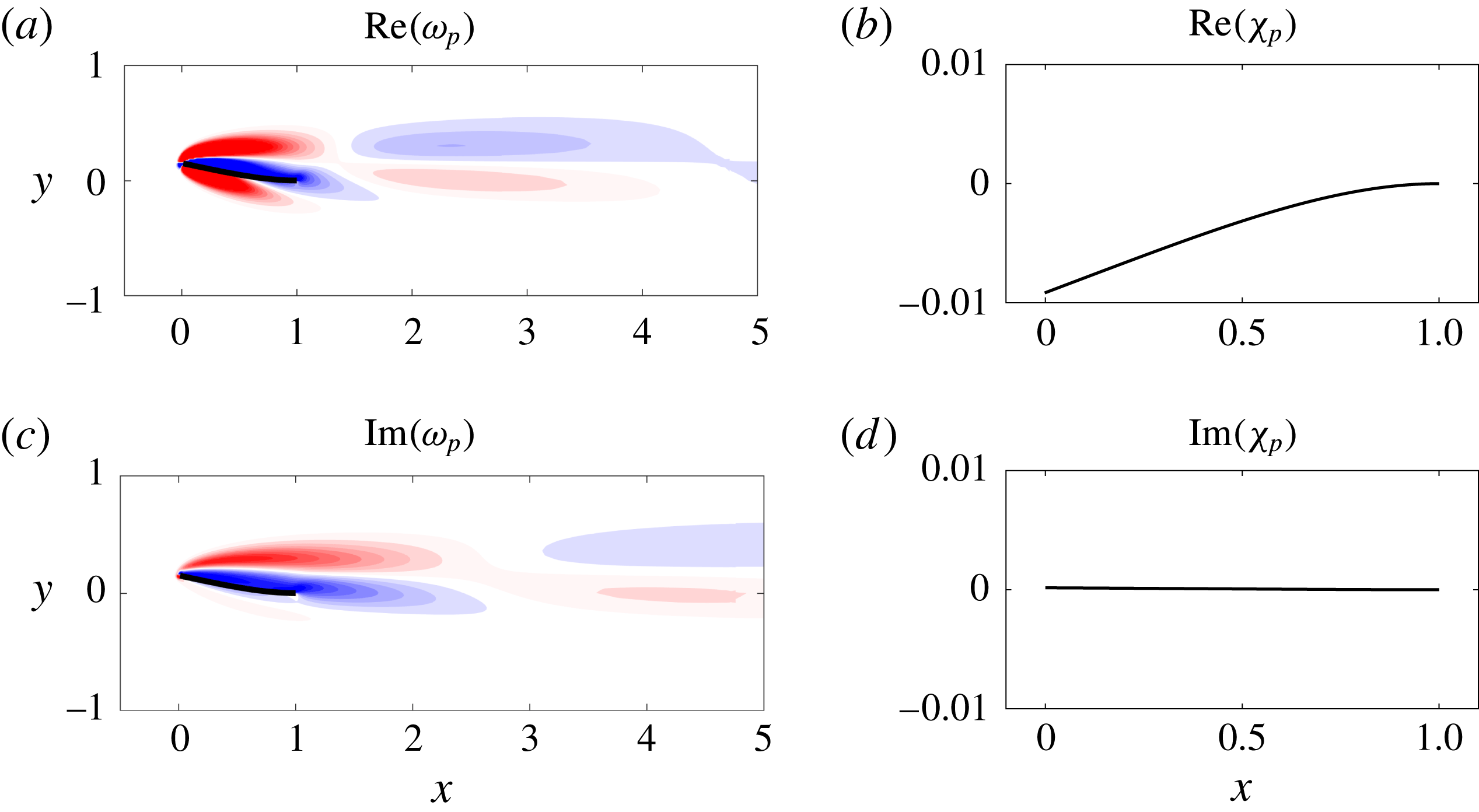
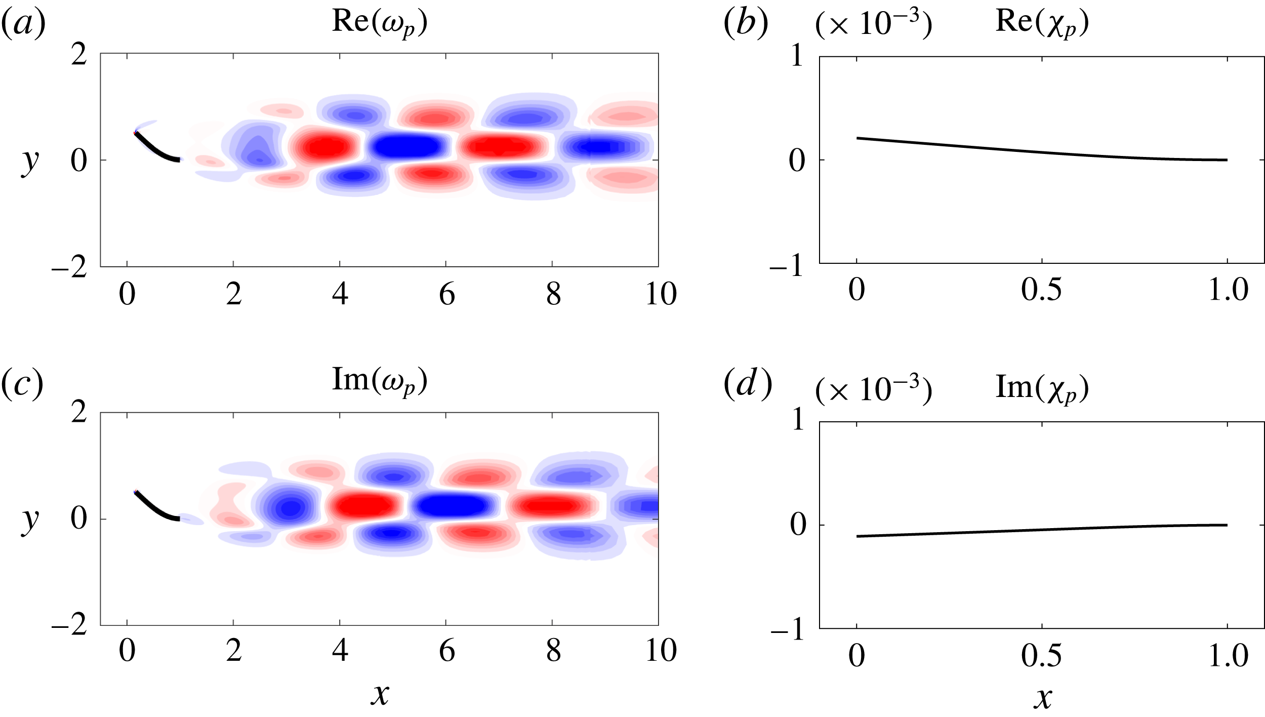
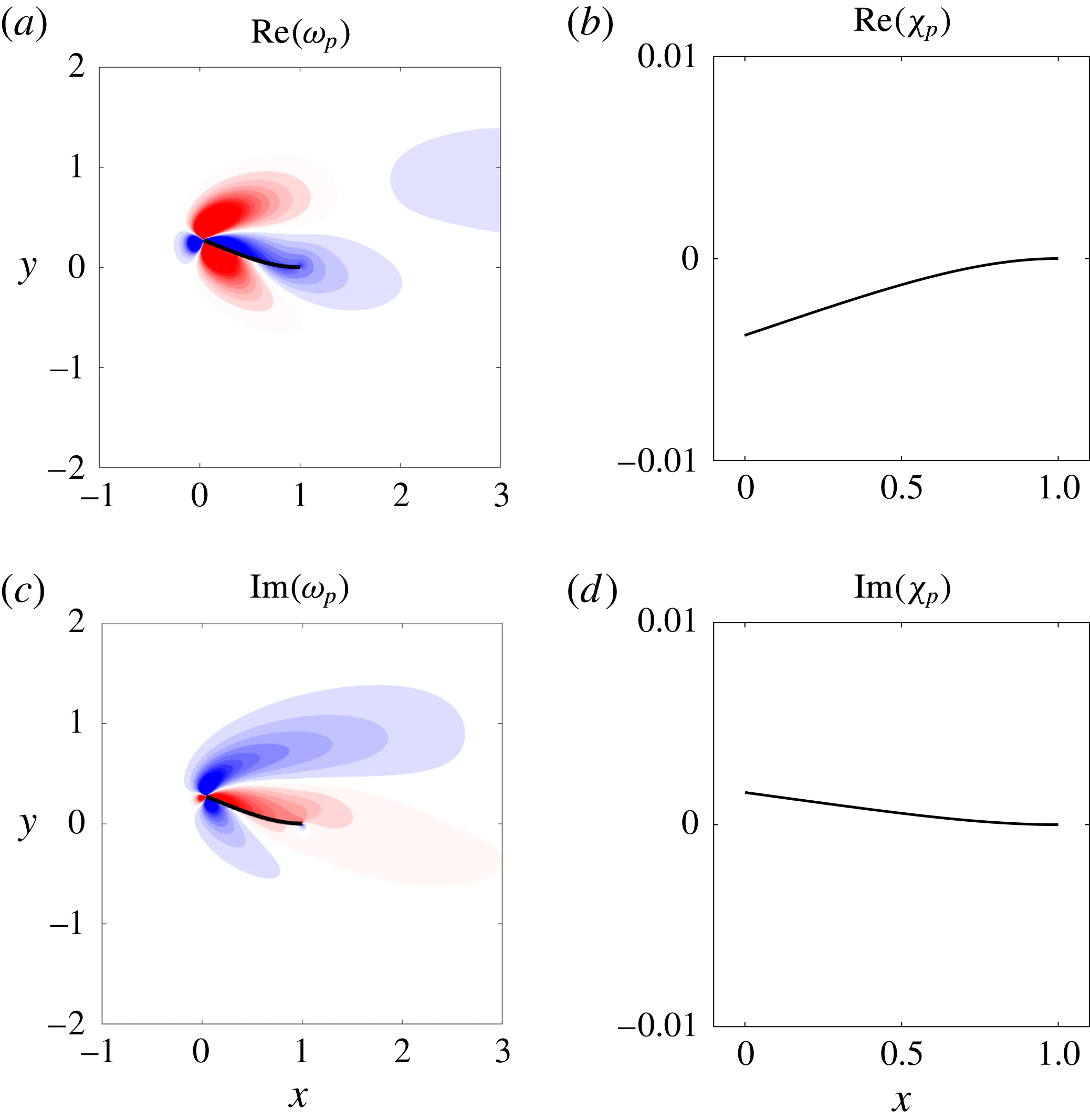
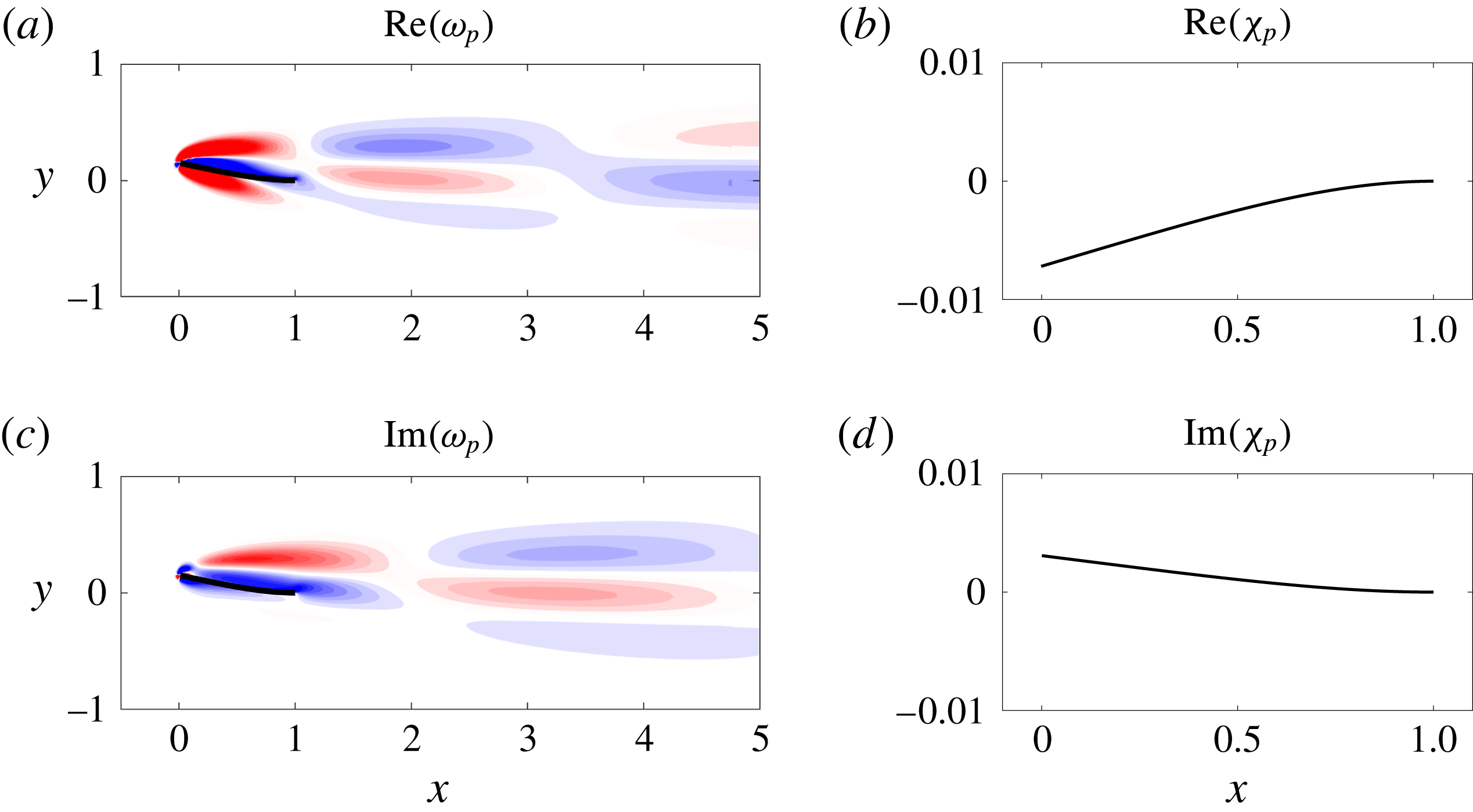
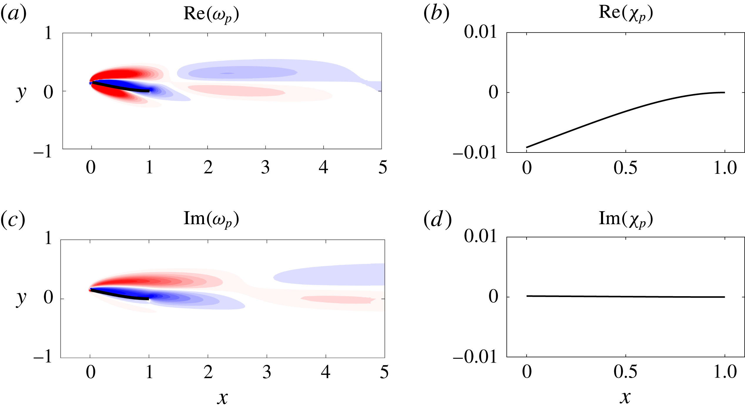
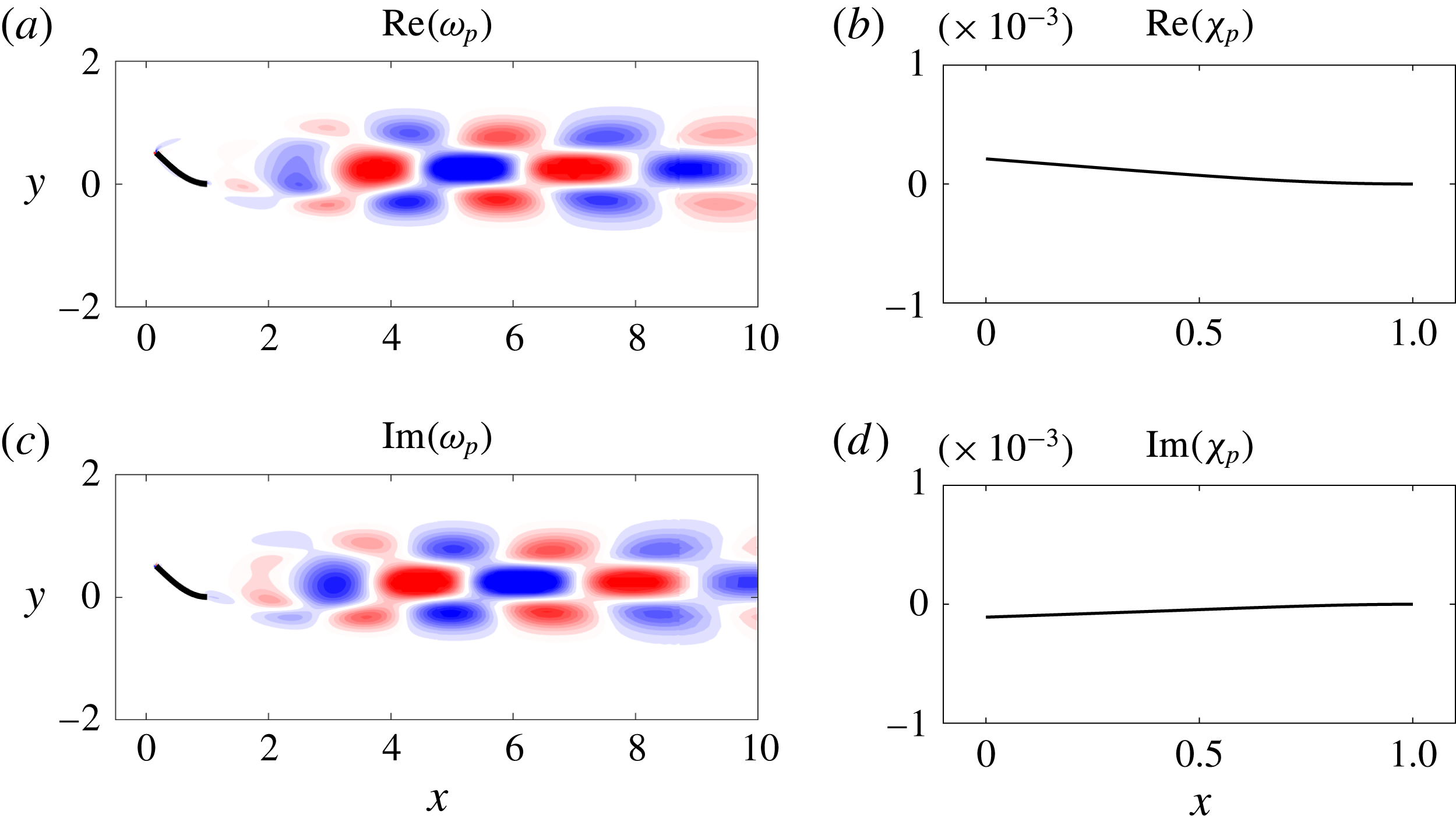
Figures 7 and 8 show the leading mode of the deformed equilibrium near the critical stiffness values where bifurcation occurs for
 $M_{\unicode[STIX]{x1D70C}}=0.5$
and
 $M_{\unicode[STIX]{x1D70C}}=5$
, respectively. The similarities between the figures suggest that the same underlying mechanism is responsible for the onset of small-deflection flapping at these different mass ratios. The mode is decomposed into real and imaginary parts, which highlights the time dependence of the vortex motion. Note that the left panels of figures 7 and 8 appear to indicate vortex shedding, but the global modes are the difference between the complete flow field and the base flow (for small times before nonlinearities take effect). As such, an interpretation of the total flow field in terms of vortex shedding cannot be deduced from these figures. Vortex shedding is not evident in figure 6.
In both figures 7 and 8, the vortical structures are most pronounced near the flag and decay in strength downstream of the flag. This demonstrates the importance of the flag in driving flapping motion in this regime. This is in contrast to the deformed-mode regime described in § 3.5, which is driven by vortex shedding that is triggered by a flow instability (cf. figure 17); the strength of individual vortices far downstream of the flag in figure 17 is notable compared with that of figures 7 and 8. As the flag mass increases, the oscillation frequency of small-deflection flapping decreases (cf. figure 5). This coincides with vorticity formation over longer time scales that manifests itself in the form of elongated wake structures (cf. figures 7 and 8).
Real (a,b) and imaginary (c,d) parts of vorticity (a,c) and flag displacement (b,d) of the leading global mode of the deformed equilibrium for
 $M_{\unicode[STIX]{x1D70C}}=0.5,K_{B}=0.41$
and
 $Re=200$
(corresponding to small-deflection flapping). Vorticity contours are in 20 increments from
 $-$
0.05 to 0.05. For visual clarity, the flag is plotted in the deformed-equilibrium state in (a,c) and in the perturbed state (with the equilibrium subtracted) in (b,d).
Real (a,b) and imaginary (c,d) parts of vorticity (a,c) and flag displacement (b,d) of the leading global mode of the deformed equilibrium for
 $M_{\unicode[STIX]{x1D70C}}=5,K_{B}=0.41$
and
 $Re=200$
(corresponding to small-deflection flapping). Vorticity contours are in 20 increments from
 $-$
0.2 to 0.2. For visual clarity, the flag is plotted in the deformed-equilibrium state in (a,c) and in the perturbed state (with the equilibrium subtracted) in (b,d).
3.3 Large-amplitude flapping
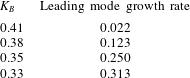
Decreasing stiffness in the small-deflection flapping regime is associated with an increasingly unstable leading mode (see table 3) and a corresponding increase in flapping amplitude. Eventually, the amplitude is sufficiently large for the flag to reach past the centreline (
 $\unicode[STIX]{x1D6FF}_{tip}=0$
) position, and large-amplitude flapping ensues.
Growth rate of the leading global mode of the deformed equilibrium for
 $M_{\unicode[STIX]{x1D70C}}=0.5$
for stiffnesses in the small-deflection flapping and large-amplitude flapping regimes.
At this Reynolds number of
 $Re=200$
, the large-amplitude behaviour is associated with sufficient bluffness to the flow that vortex shedding occurs. The resulting dynamics is dependent on flag mass, and we therefore consider it separately in what follows.
3.3.1 Light flags: potential for classical VIV, and breakdown of classical VIV as a route to chaos
For sufficiently light flags (
 $M_{\unicode[STIX]{x1D70C}}\leqslant 0.5$
in our study), large-amplitude flapping was shown to correspond to specific vortex-shedding patterns (Gurugubelli & Jaiman Reference Gurugubelli and Jaiman2015; Ryu et al.
Reference Ryu, Park, Kim and Sung2015; Shoele & Mittal Reference Shoele and Mittal2016), and Sader et al. (Reference Sader, Cossé, Kim, Fan and Gharib2016a
) used experiments and a scaling analysis to argue that classical VIV could occur. We explain here the previously observed shedding patterns in connection to classical VIV. We show that for a range of stiffnesses (
 $2.5\lesssim 1/K_{B}\lesssim 3.8$
) the P
 $+$
P shedding pattern occurs and the system exhibits classical VIV behaviour. With decreasing stiffness (
 $3.8\lesssim 1/K_{B}\lesssim 4.4$
), however, there is a breakdown in classical VIV and a corresponding change in shedding behaviour that serves as a precursor to the chaotic regime discussed in § 3.4.
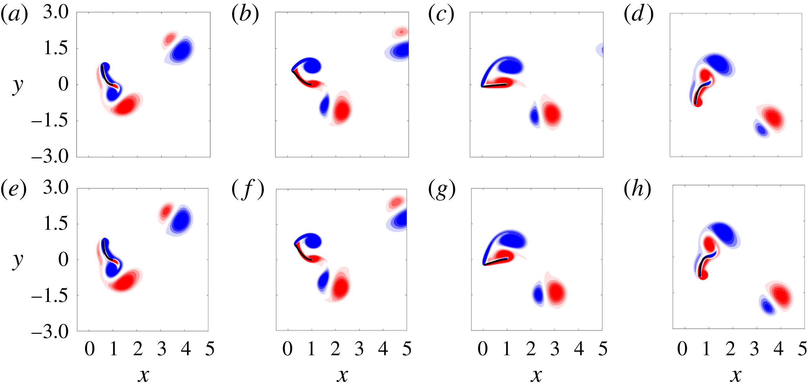
To illustrate the synchronisation of vortex shedding and flapping in the classical VIV regime (
 $2.5\lesssim 1/K_{B}\lesssim 3.8$
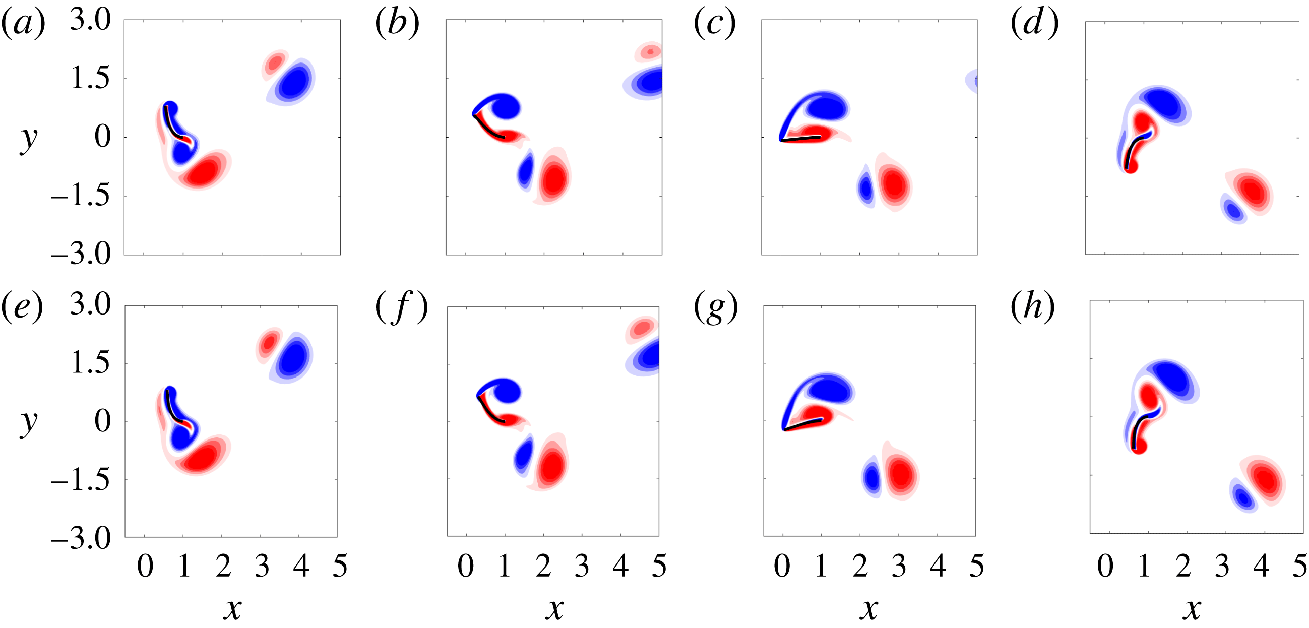
), we show snapshots from a half-period of large-amplitude flapping for
 $M_{\unicode[STIX]{x1D70C}}=0.05,0.5$
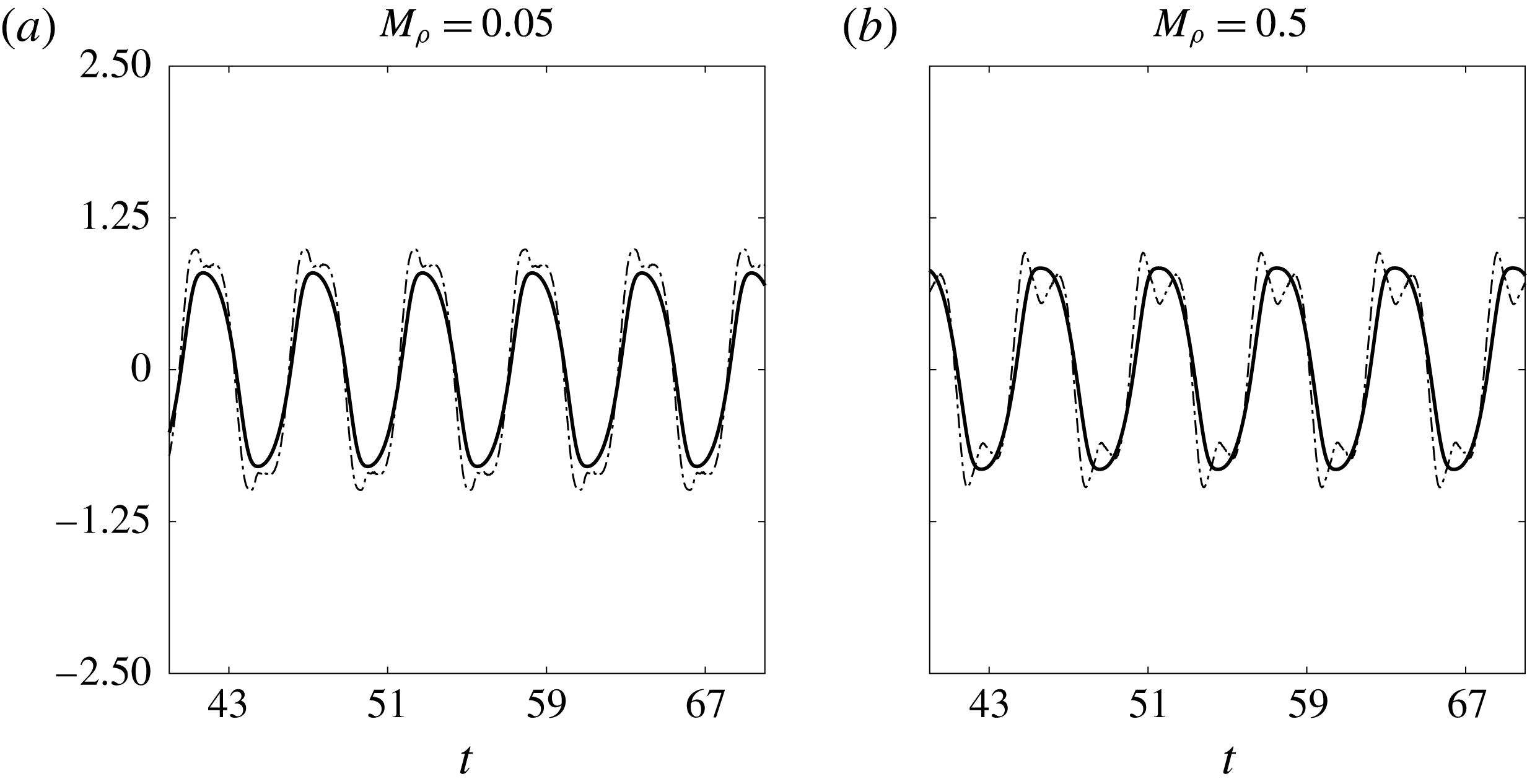
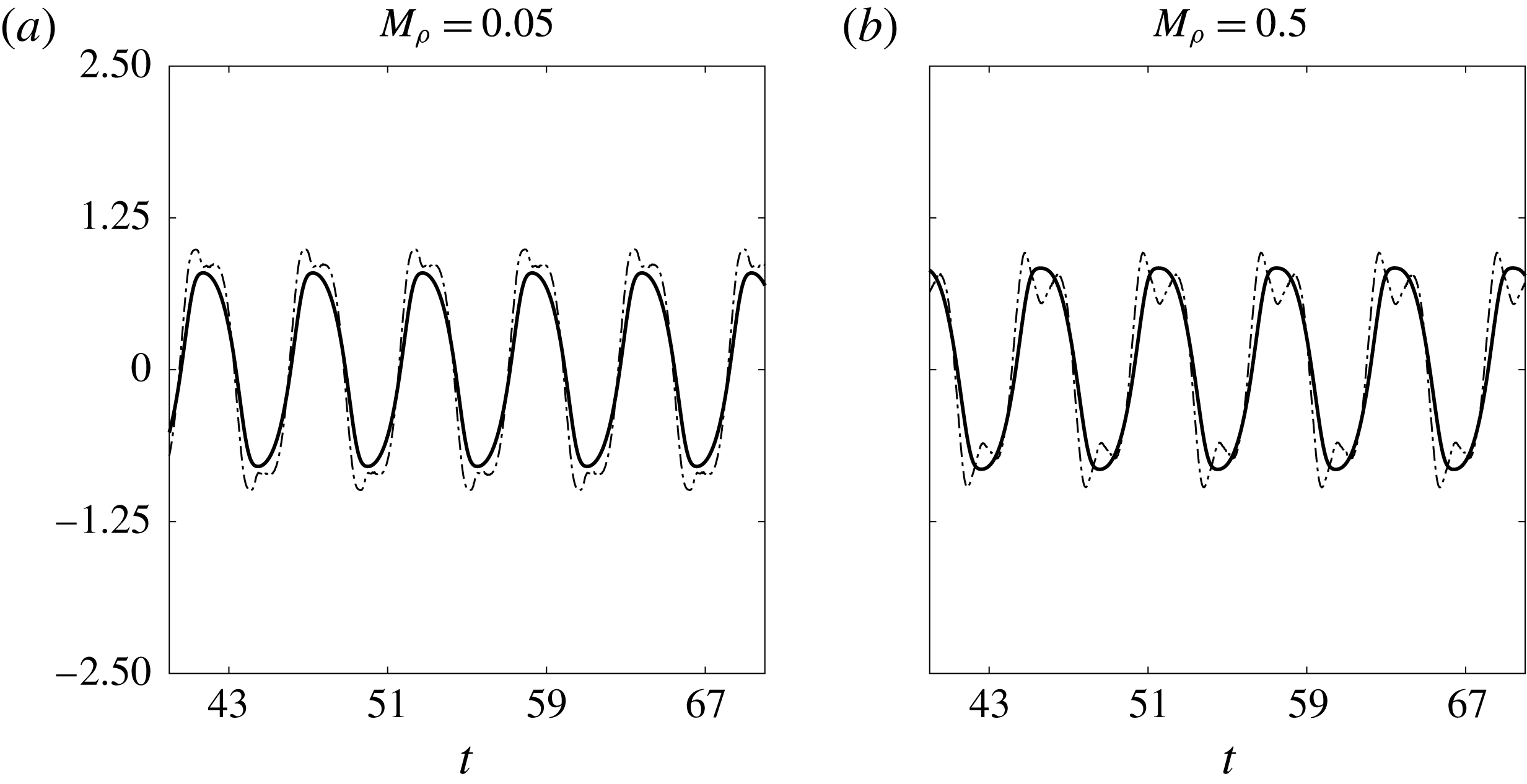
in figure 9. Note that despite an order of magnitude change in mass ratio, the vortex-shedding patterns in the two rows of the figure are similar: when the flag reaches its peak amplitude the leading-edge vortex formed during the upstroke grows (a,e); as the flag begins its downstroke the leading-edge vortex is released and a trailing-edge vortex forms (b,f); the vortices grow in size as the flag reaches its centreline position (c,g); while the leading- and trailing-edge vortices advect downstream to form a P vortex pair (see Williamson & Roshko (Reference Williamson and Roshko1988) for a description of this vortex characterisation), a leading-edge vortex forms as the flag continues its downstroke (d,h). When the flag reaches its peak position, an analogous process to the one just described occurs during the upstroke (with oppositely signed vorticity). To confirm that this regime corresponds to classical VIV, we show in figure 10 time traces of the coefficient of lift and tip displacement for
 $M_{\unicode[STIX]{x1D70C}}=0.05,0.5$
. The lift and tip displacement are synchronised, and therefore satisfy the definition of VIV (Khalak & Williamson Reference Khalak and Williamson1999; Sarpkaya Reference Sarpkaya2004); see § 1.
Vorticity contours at four snapshots of a flapping period of a flag in large-amplitude flapping for
 $M_{\unicode[STIX]{x1D70C}}=0.05$
(a) and
 $M_{\unicode[STIX]{x1D70C}}=0.5$
(b). The other parameters were
 $Re=200,K_{B}=0.32$
. Contours are in 18 increments from
 $-$
5 to 5.
Tip displacement (——) and coefficient of lift (— ⋅ —) for an inverted flag in large-amplitude flapping with
 $Re=200$
,
 $K_{B}=0.32$
.
Ryu et al. (Reference Ryu, Park, Kim and Sung2015) showed that there are other possible vortex shedding patterns in large-amplitude flapping for light flags, i.e. for small mass ratios,
 $M_{\unicode[STIX]{x1D70C}}$
. We demonstrate here that these new patterns (occurring for
 $3.8\lesssim 1/K_{B}\lesssim 4.4$
) correspond to a breakdown in classical VIV behaviour. One pattern identified by Ryu et al. (Reference Ryu, Park, Kim and Sung2015) is the 2P
 $+$
2P pattern, which occurs for
 $M_{\unicode[STIX]{x1D70C}}=0.5$
and
 $K_{B}=0.23$
(corresponding to the rightmost set of markers in region IV of the bifurcation diagram in figure 3
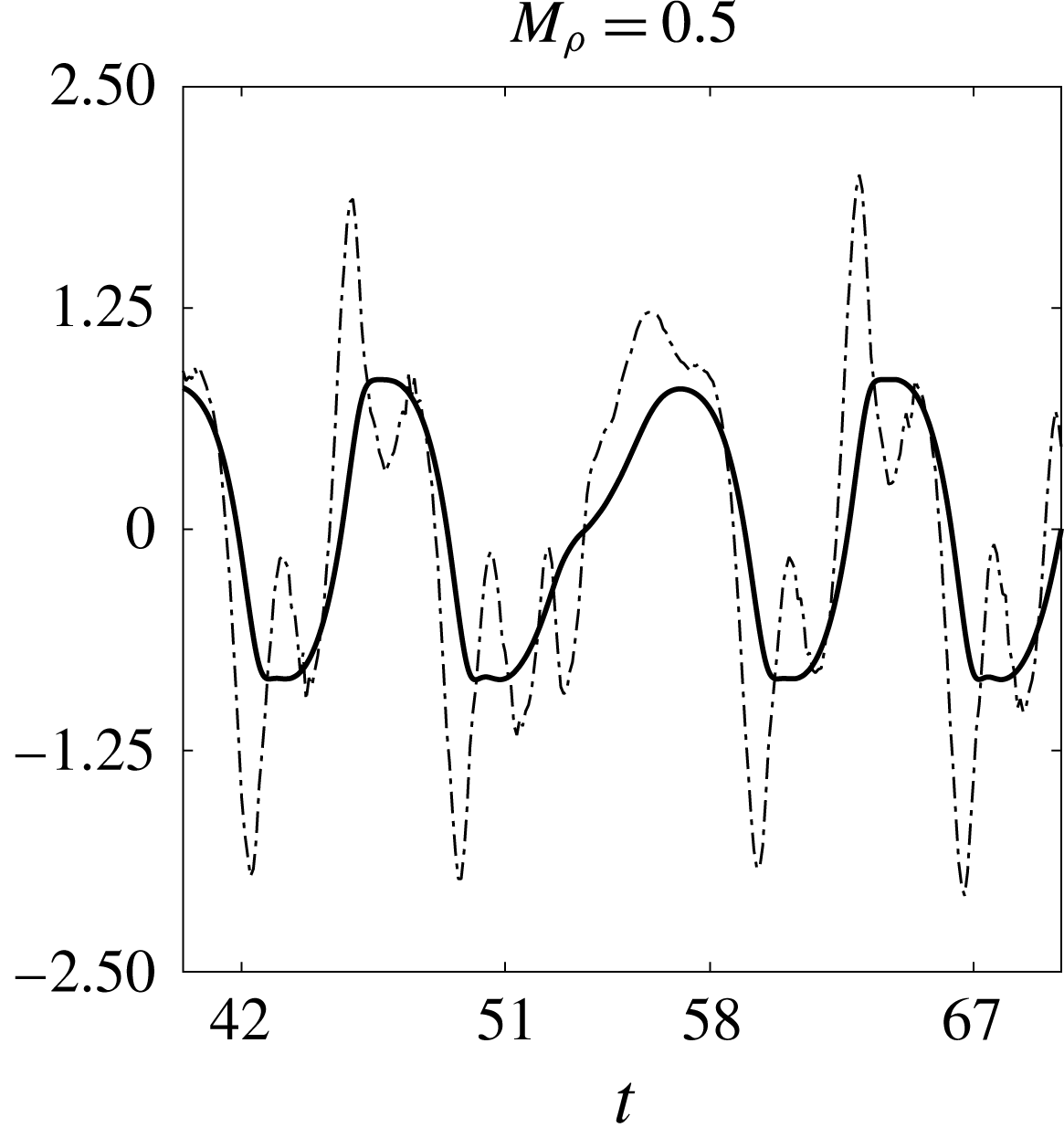
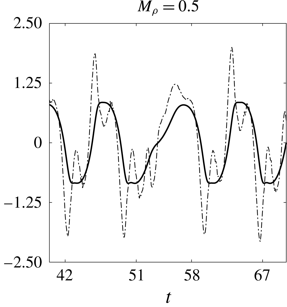
b). This pattern is shown in figure 11. Figure 12 illustrates the corresponding coefficient of lift and tip displacement for this set of parameters. From this figure, a disruption of the underlying periodic flapping motion (occurring over
 $51\lesssim t\lesssim 58$
) is evident where the lift and tip displacements desynchronise. This departure from limit-cycle behaviour can also be seen from the bifurcation diagrams in figure 3(a,b), as there are multiple markers at a given stiffness in the range
 $3.8\lesssim 1/K_{B}\lesssim 4.4$
.
Vorticity contours at four snapshots of a flapping period of a flag in large-amplitude flapping for
 $Re=200$
,
 $M_{\unicode[STIX]{x1D70C}}=0.5$
, and
 $K_{B}=0.23$
. Contours are in 18 increments from
 $-$
5 to 5.
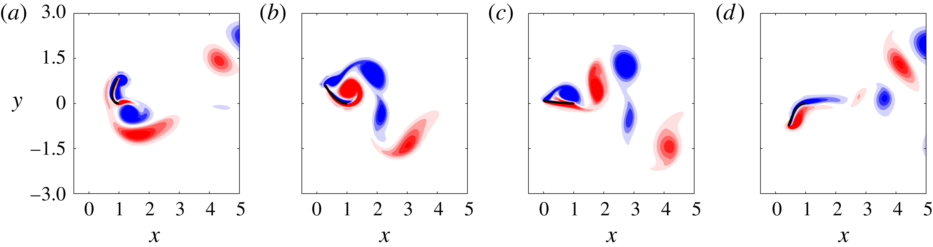
Tip displacement (——) and coefficient of lift (— ⋅ —) for an inverted flag in large-amplitude flapping with
 $Re=200$
,
 $M_{\unicode[STIX]{x1D70C}}=0.5$
, and
 $K_{B}=0.23$
.
The potential for large-amplitude flapping with and without classical VIV is indicative of the dominant role of fluid convection, relative to the structure, in the dynamics of light flags (small
 $M_{\unicode[STIX]{x1D70C}}$
) in large-amplitude flapping. Over a range of stiffnesses (
 $2.5\lesssim 1/K_{B}\lesssim 3.8$
), the natural frequency of the sheet is sufficiently close to that of the bluff-body wake instability that the two synchronise to form a classical VIV; see Sader et al. (Reference Sader, Cossé, Kim, Fan and Gharib2016a
). The entire system progresses in limit-cycle dynamics at a uniform frequency. From the frequency plots in figure 5(a,b), the frequency can be seen to be near a Strouhal number of 0.2 when normalised using the projected length of the flag to the flow at the peak flapping amplitude. With decreasing stiffness, however, the flapping frequency decreases (see figure 5) and vortex shedding can no longer synchronise with flapping. This disruption to classical VIV is associated with a breakdown in limit-cycle dynamics (i.e. aperiodicity) and additional vortices shed per cycle – this provides a route to chaotic flapping (as will be discussed in more detail in § 3.4). By contrast, fluid convection is less important in setting the dynamics for heavy flags, as discussed in the next subsection.
3.3.2 Heavy flags: not classical VIV
We now examine large-amplitude flapping for large mass ratios (
 $M_{\unicode[STIX]{x1D70C}}=5,50$
). As was seen for lighter flags, various shedding patterns can be obtained at these mass ratios for different stiffnesses. However, there are no values of stiffness for which these heavy flags undergo classical VIV. Rather than catalogue all possible shedding patterns, we consider characteristic examples at the stiffness of
 $K_{B}=0.32$
to facilitate our discussion.
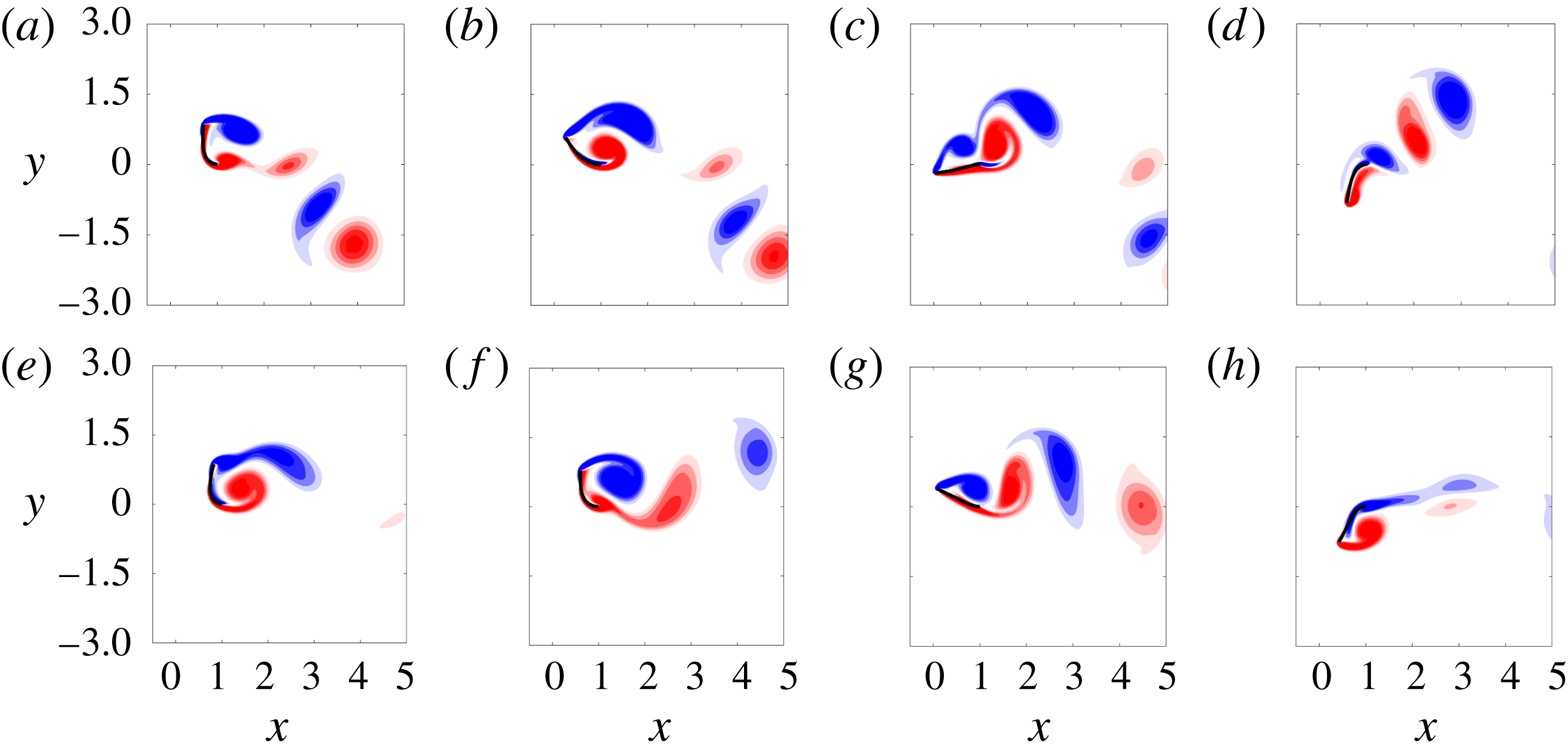
Figure 13 shows a half-cycle of flapping for
 $M_{\unicode[STIX]{x1D70C}}=5,50$
. The
 $M_{\unicode[STIX]{x1D70C}}=5$
case (figure 13
a–d) is seen to lead to a P
 $+$
S wake structure per half-cycle. For
 $M_{\unicode[STIX]{x1D70C}}=50$
(figure 13
e–h), even more vortices are shed during the downstroke: the first leading- and trailing-edge vortices are shed when the flag is still near its peak amplitude (e); the flag begins its downstroke and another leading- and trailing-edge vortex pair are formed (f); as the flag nears its centreline position, a third leading-edge vortex forms (g); this leading-edge vortex combines with a newly formed trailing-edge vortex during the downstroke phase to form a third pair that is advected downstream; at the end of the downstroke phase, new vortices form at the leading and trailing edge as the flag reaches its peak amplitude (h).
Vorticity contours at four snapshots of a flapping period of a flag in large-amplitude flapping for
 $M_{\unicode[STIX]{x1D70C}}=5$
(a) and
 $M_{\unicode[STIX]{x1D70C}}=50$
(b). The other parameters were
 $Re=200,K_{B}=0.32$
. Contours are in 18 increments from
 $-$
5 to 5.
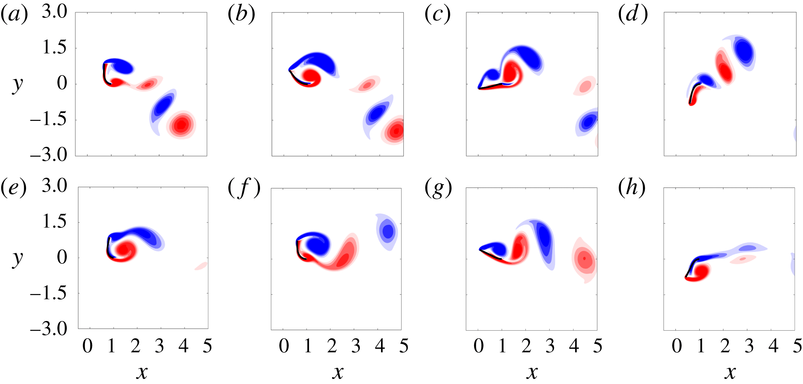
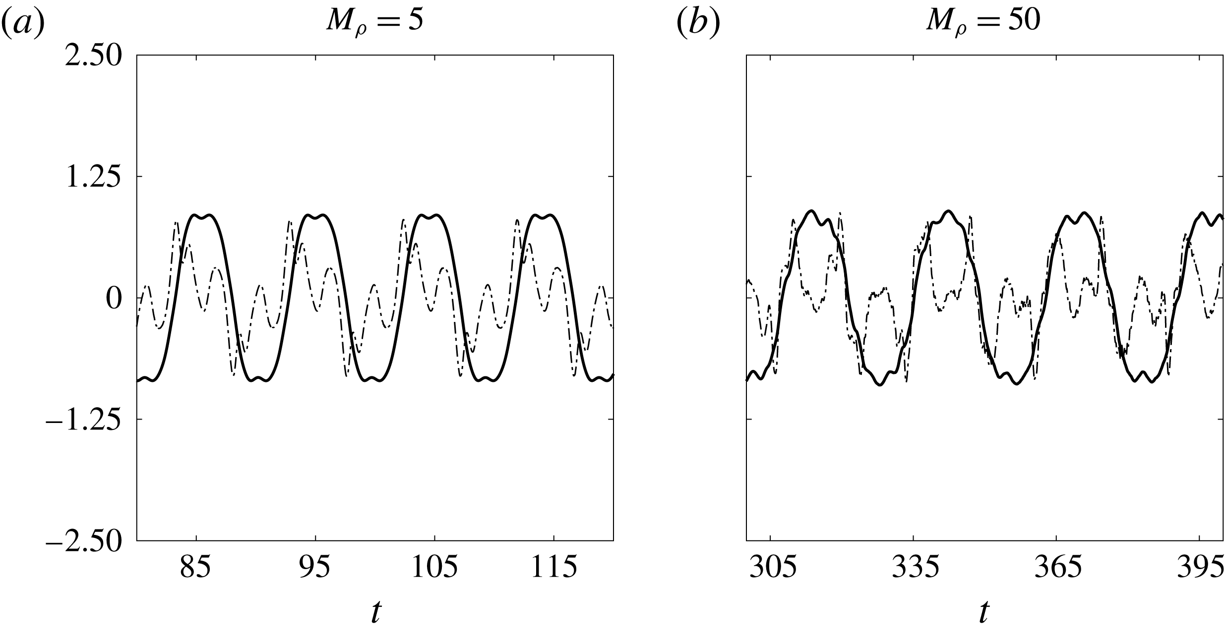
The disparate time scales between vortex shedding and flapping is illustrated further through time traces of the coefficient of lift and tip displacement (see figure 14). For both mass ratios, the dominant frequency of the coefficient of lift is higher than that of the tip displacement. Moreover, for
 $M_{\unicode[STIX]{x1D70C}}=50$
there is a departure from periodicity that can be observed in figure 14 (and is reflected in the bifurcation diagram in figure 3
d). These observations reflect that heavy flags do not undergo classical VIV – a result predicted by Sader et al. (Reference Sader, Cossé, Kim, Fan and Gharib2016a
) through a scaling analysis.
Tip displacement (——) and coefficient of lift (— ⋅ —) for an inverted flag in large-amplitude flapping with
 $Re=200$
,
 $K_{B}=0.32$
.
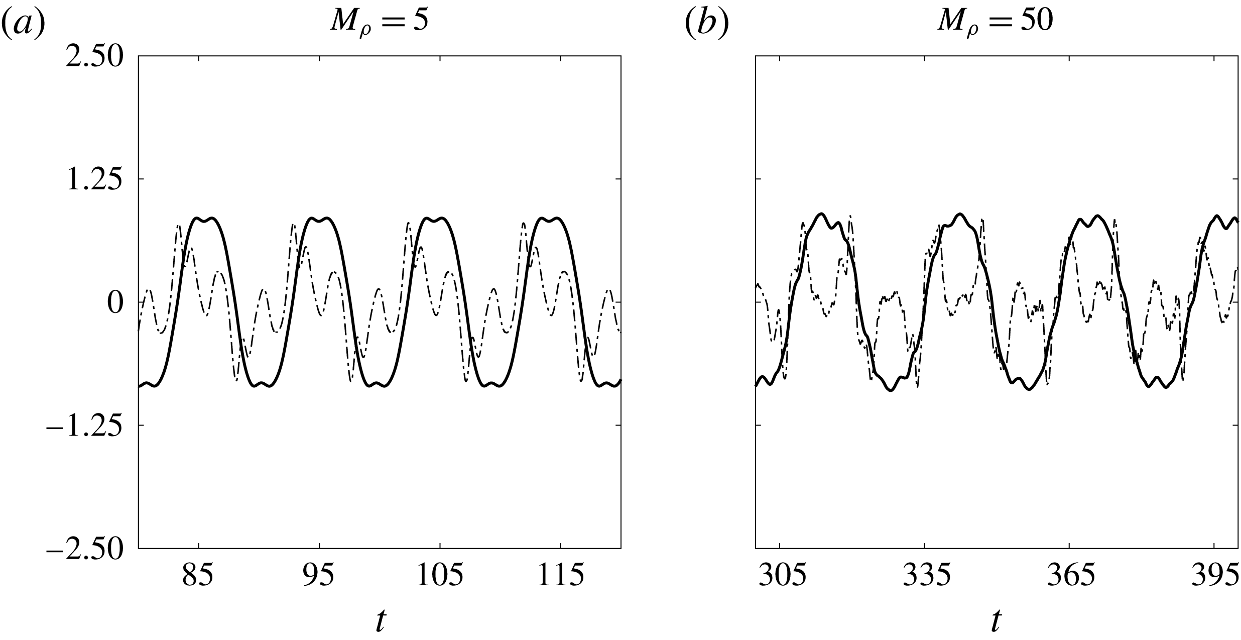
For
 $M_{\unicode[STIX]{x1D70C}}=5$
, it is clear from figure 14 that the lift coefficient has a subdominant frequency at the dominant flag-flapping frequency. Thus, it is possible that the large-amplitude response is a result of synchronisation between flapping and a higher-harmonic response in the fluid. This relation between the dominant flapping motion and a higher-harmonic fluid response could also be occurring for
 $M_{\unicode[STIX]{x1D70C}}=50$
, although the observed aperiodicity in the system could be reflective of ‘galloping-type’ lift mechanism. Future work could further investigate the mechanisms driving flapping when classical VIV is absent.
While the specific relationship between vortex shedding and flapping in this regime remains an open question, the frequency plots in figure 5(c,d) provides insight into the physics. The plots show that the frequency scaling is similar to the (linear) natural frequency of a sheet in an inviscid fluid (solid curves). This natural frequency is computed using the theory of Shen et al. (Reference Shen, Chakraborty and Sader2016), which accounts for added mass of the fluid (though for these high mass ratios this effect is negligible and the natural frequency is nearly identical to that in a vacuum). There is a downward shift between the flapping frequency and the natural frequency prediction of Shen et al. (Reference Shen, Chakraborty and Sader2016), although this is expected because the latter does not account for viscosity, which would lower the natural frequency. These results show that large-amplitude flapping is structure-dominated for large mass ratios, as expected.
3.4 Chaotic flapping
For sufficiently light flags (
 $M_{\unicode[STIX]{x1D70C}}\leqslant 0.5$
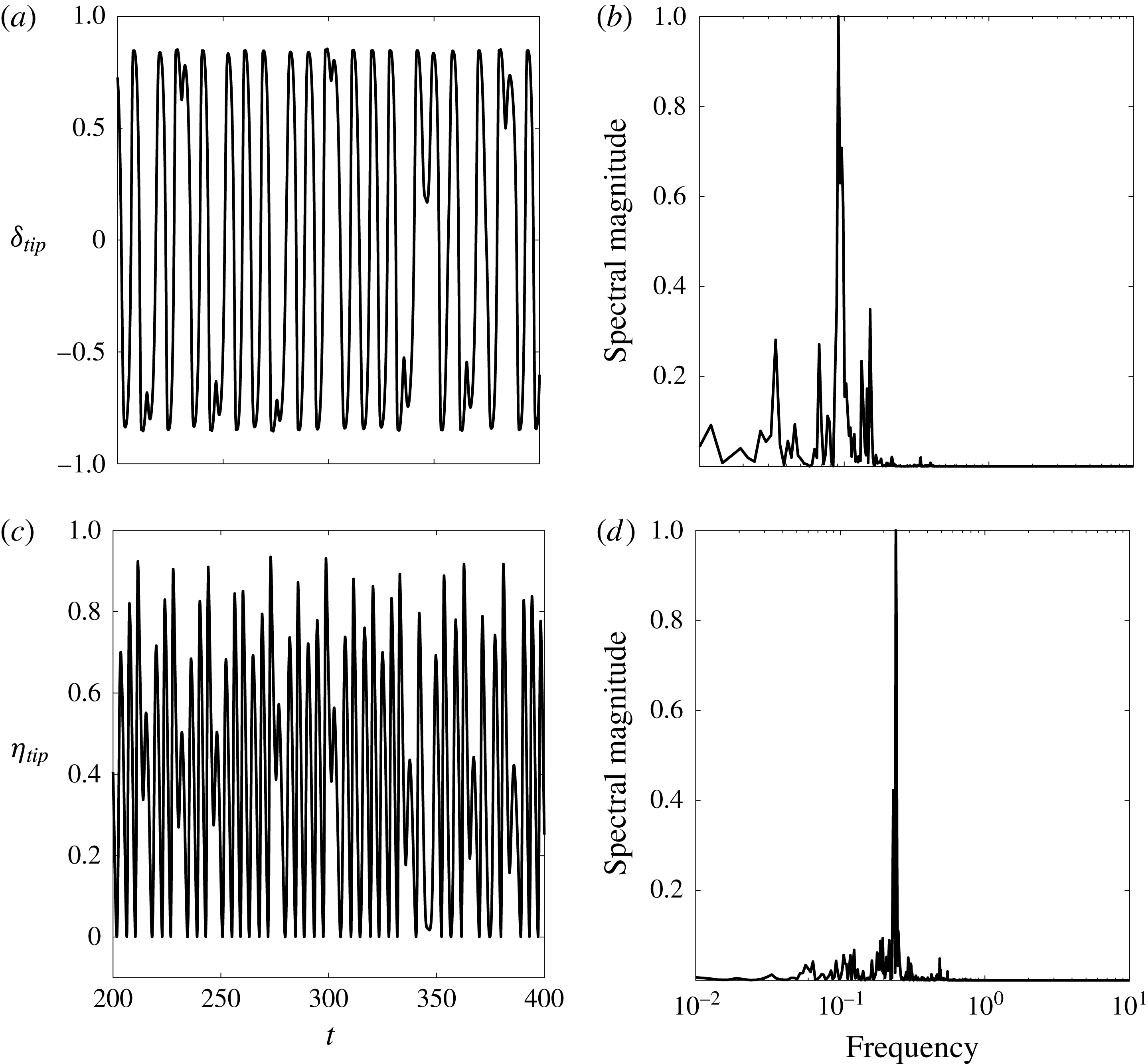
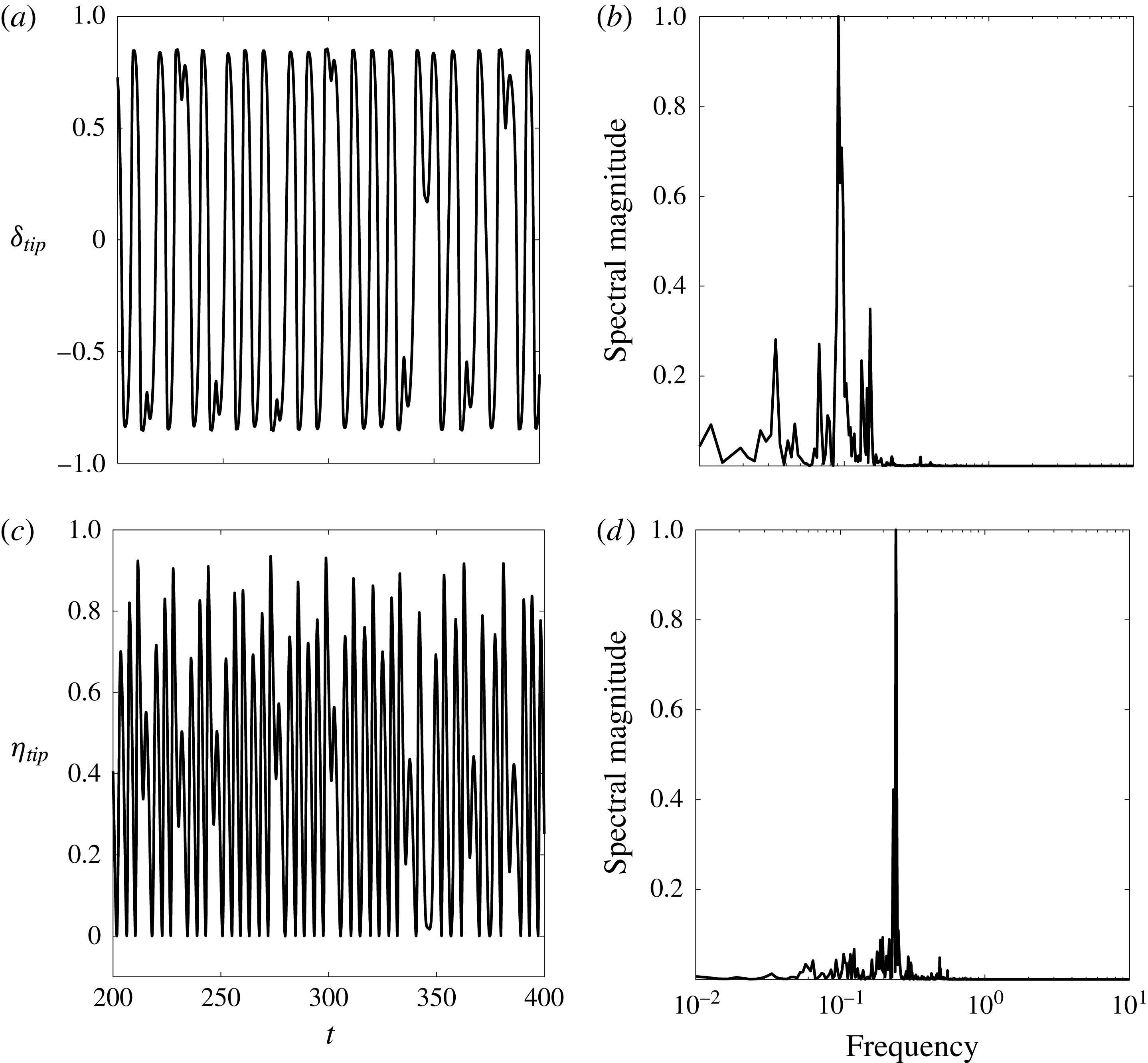
in our studies), large-amplitude flapping (region IV in figure 3) bifurcates to chaotic flapping (region V) before entering into deflected-mode flapping (region VI). Figure 15 shows that the time traces of both the transverse and streamwise tip displacement are aperiodic and associated with broadband frequency content (note that we use
 $\unicode[STIX]{x1D702}_{tip}(t)$
to denote the streamwise tip displacement in the figure).
(a,c) Tip displacement as a function of time in the transverse (a,b) and streamwise (c,d) directions; (b,d) corresponding spectral density computations (computed over the time window
 $t\in [20,500]$
). All plots correspond to a flag in the chaotic flapping regime, with
 $M_{\unicode[STIX]{x1D70C}}=0.05,K_{B}=0.17,Re=200$
.
To demonstrate mathematically that this behaviour is chaotic, we compute the Lyapunov exponent of the system using the time-delay method of Wolf et al. (Reference Wolf, Swift, Swinney and Vastano1985). The method uses a time-delay procedure from a small subset of the full state to reconstruct a higher-dimensional state space, and provides an approximation of the distance,
 $d(t)$
, of two trajectories starting close to one another at an initial time
 $t_{0}$
in this higher-dimensional state space. In this work, a ten-dimensional reconstruction is made from time information of the transverse velocity-displacement data. The same approach was used by Connell & Yue (Reference Connell and Yue2007) to identify chaotic flapping of conventional flags. The evolution of the distance
 $d(t)$
is written as
 $$\begin{eqnarray}\displaystyle d(t)=d(t_{0})\text{e}^{\unicode[STIX]{x1D6FE}(t-t_{0})}, & & \displaystyle\end{eqnarray}$$
where
 $\unicode[STIX]{x1D6FE}$
is the Lyapunov exponent that represents the departure or convergence of the two trajectories. A zero value of
 $\unicode[STIX]{x1D6FE}$
corresponds to a stationary state where the system is in limit cycle behaviour; a positive value of
 $\unicode[STIX]{x1D6FE}$
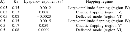
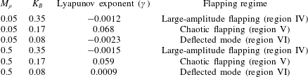
corresponds to divergence of the two trajectories, and thus to chaotic flapping. Table 4 shows the Lyapunov exponent computed for various values of
 $M_{\unicode[STIX]{x1D70C}}$
and
 $K_{B}$
. For large-amplitude and deflected-mode flapping, the exponent is approximately zero (
 ${\sim}$
of order
 $10^{-3}$
), coincident with limit-cycle flapping. In the chaotic regime that occurs at stiffnesses between large-amplitude and deflected-mode flapping, the exponent is positive and larger by over an order of magnitude (
 ${\sim}$
of order 0.1), indicative of a transition to chaotic behaviour in this regime.
Lyapunov exponents for different flapping regimes. For each regime, the corresponding region from the bifurcation diagram of figure 3 is indicated in parentheses.
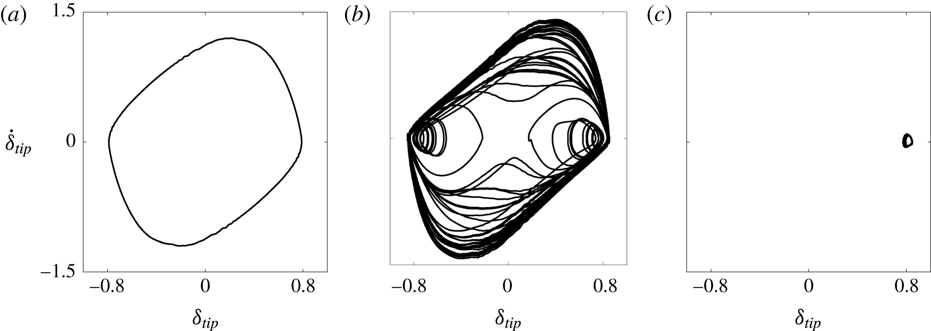
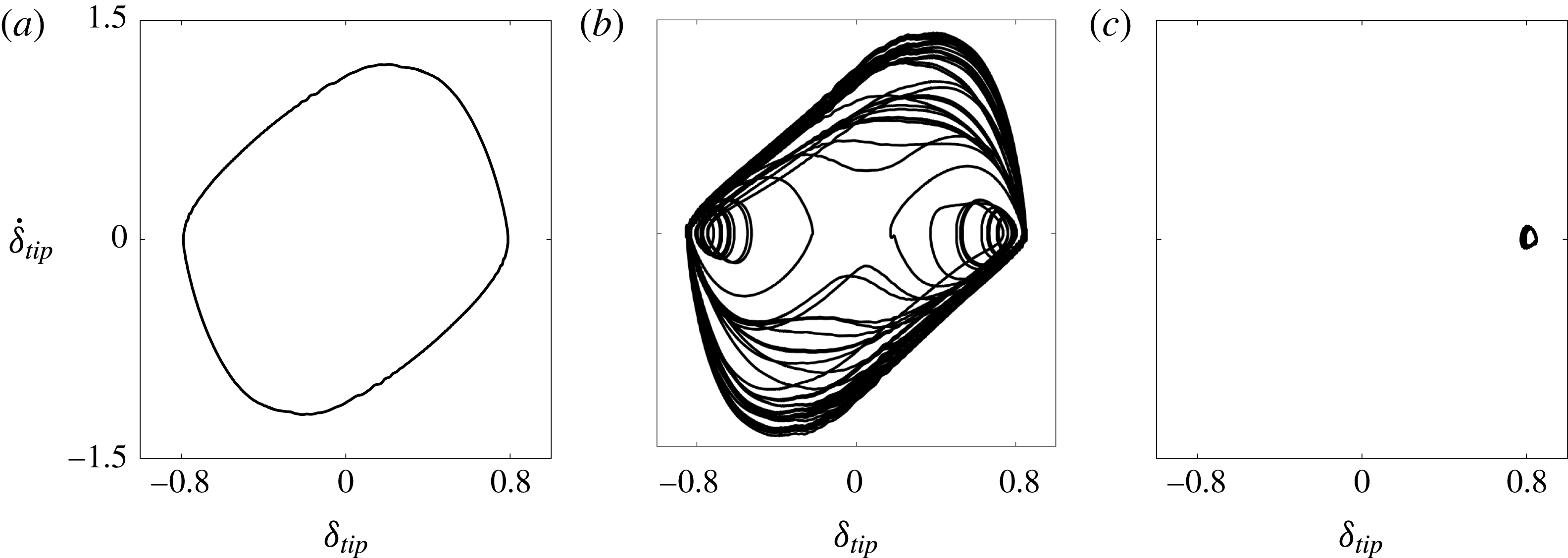
To elucidate the nature of chaotic flapping, we show in figure 16 phase portraits of tip velocity versus tip displacement for inverted flags in the large-amplitude flapping, chaotic flapping, and deflected-mode regimes. The figures demonstrate that the chaotic flapping phase portrait contains both the large periodic orbit of large-amplitude flapping and the small-amplitude large-deflection periodic orbit of deflected-mode flapping. Thus, the chaotic attractor contains features of both large-amplitude flapping and the deflected mode – both of which are unstable in this regime. The chaotic nature of the regime is associated with the apparent randomness in switching between these two orbits and a sensitive dependence on initial conditions (see above).
Tip-velocity displacement phase portraits for
 $M_{\unicode[STIX]{x1D70C}}=0.05$
and
 $K_{B}=0.32$
(a),
 $K_{B}=0.17$
(b) and
 $K_{B}=0.11$
(c).
The bifurcation diagrams in figure 3 demonstrate that increasing the mass ratio reduces the chaotic behaviour. In moving from
 $M_{\unicode[STIX]{x1D70C}}=0.05$
to
 $M_{\unicode[STIX]{x1D70C}}=0.5$
, there were certain stiffnesses within the chaotic flapping regime that exhibited periodic flapping instead of chaotic flapping (see figure 3). This may be an artefact of only running the simulations for finite time, but the absence of chaotic flapping over a minimum of 55 flapping periods for certain stiffnesses at
 $M_{\unicode[STIX]{x1D70C}}=0.5$
speaks to the effect of increasing flag inertia on reducing the chaotic behaviour. It could be that islands of periodicity exist within the chaotic regime, as has been observed for other unrelated dynamical systems (Strogatz Reference Strogatz1994). For the heavier flag cases of
 $M_{\unicode[STIX]{x1D70C}}=5,50$
, chaotic flapping is not observed in any of the simulations. Thus, chaotic flapping appears to only be associated with mass ratios (
 $M_{\unicode[STIX]{x1D70C}}$
) for which classical VIV flapping occurs.
The relationship between chaotic flapping and classical VIV can be understood from the results of § 3.3. We first consider light flags (
 $M_{\unicode[STIX]{x1D70C}}<1$
) in the large-amplitude flapping regime. Decreasing the stiffness reduces the resonant frequency of the flag. This increases the disparity between the natural frequency of vortex shedding (if lock-on were not present) and the flag’s resonant frequency. When this discrepancy increases further, the lock-on phenomenon is disrupted. This causes the flag to spend considerable time near the deflected mode, which at this point is only weakly unstable – a small decrease in stiffness causes a transition to the deflected-mode state. Such weakly unstable behaviour of the deflected-mode regime is evident in figure 15 (and in figure 11 of Sader et al. (Reference Sader, Cossé, Kim, Fan and Gharib2016a
)). This mechanism is what leads to a sensitive dependence on initial conditions, i.e. chaos.
In contrast, heavy flags (
 $M_{\unicode[STIX]{x1D70C}}>1$
) do not exhibit classical VIV. The vortex-shedding frequency is much higher than the natural resonant frequency of the flag, and lock-on is not favoured. Thus, a mechanism for disruption of classical VIV is not possible since classical VIV is absent to begin with for heavy flags.
Note also the distinction between chaotic flapping of inverted flags and conventional flags. Connell & Yue (Reference Connell and Yue2007) demonstrated that for conventional flags the mass ratio controls chaos, which arises once this parameter becomes sufficiently high because of the increased flag inertia. By contrast, for inverted flags chaos occurs due to the combined effects of disparity between the natural vortex shedding frequency and resonant frequency of the flag, and a weakly unstable deflected-mode state. Chaos therefore serves as a precursor to behaviour that evolves entirely on a stable attractor (the deflected-mode regime, discussed in the next section), as stiffness is further reduced. This occurrence of chaos as an intermediate state before a new regime is observed in other dynamical systems, including the Lorenz system.
3.5 Deflected-mode regime
For low stiffnesses the system transitions to a large-deflection state about which small-amplitude flapping occurs; i.e. the amplitude is much smaller than the deflection magnitude of the deformed equilibrium. As seen in figure 3, this flapping is not centred about the deformed-equilibrium position: the mean and equilibrium states are different.
The nature of flapping in this regime is qualitatively distinct from that of small-deflection flapping (region III of figure 3) and large-amplitude flapping (region IV of figure 3). Shoele & Mittal (Reference Shoele and Mittal2016) observed that when the flapping frequency is scaled by the free-stream velocity and mean tip amplitude (i.e. the mean projected length to the flow), it agrees well with the usual 0.2 value found for vortex shedding past bluff bodies (Roshko Reference Roshko1954). They used this finding to argue that the bluff-body wake instability is responsible for the small-amplitude flapping in this regime.
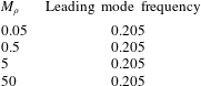
The global stability analysis of the deformed equilibrium confirms this previous conclusion. Figure 17 shows that the least damped mode is characterised by a vortical structure in the wake of the flag similar to the leading mode of a rigid stationary cylinder (Barkley Reference Barkley2006). (The analogous mode to the leading global mode for small-deflection flapping and large-amplitude flapping is also unstable in the deflected-mode regime, but is associated with a smaller growth rate.) Because vortex shedding drives the instability in the rigid cylinder, this indicates that the same destabilising mechanism exists here in the deflected mode of an inverted flag. This is in contrast to the leading mode found for small-deflection flapping and large-amplitude flapping, whose vortical structure decays in strength with distance from the flag (see the discussion in § 3.2). Moreover, as seen in table 5, the flapping frequency of this leading mode is independent of mass ratio (
 $M_{\unicode[STIX]{x1D70C}}$
). This is also distinct from the mass-dependent flapping frequency of the least damped mode for the previously discussed regimes. The similar vortical structure of the mode to other bluff-body flows and the independence of the structural parameters on the modal frequency demonstrate that the leading instability is associated with vortex shedding.
Real (a,b) and imaginary (c,d) parts of vorticity (a,c) and flag displacement (b,d) of the leading global mode of the deformed equilibrium for
 $M_{\unicode[STIX]{x1D70C}}=0.5,K_{B}=0.12$
and
 $Re=200$
. Vorticity contours are in 20 increments from
 $-$
0.2 to 0.2. The eigenvectors are identical for
 $M_{\unicode[STIX]{x1D70C}}=0.05,0.5,$
and 50.
Frequency of the leading global mode of the deformed equilibrium for
 $K_{B}=0.12$
and four different masses. All cases correspond to the deflected-mode regime.
The presence of vortex shedding in this deflected-mode regime is also the cause of the difference between the mean and equilibrium flapping positions. Vortex shedding leads to an increase in the mean lift and drag forces on the flag compared with the equilibrium state (which is devoid of vortex shedding; cf. figure 4). To demonstrate this increase in fluid forces, we ran a simulation with the flag fixed in the deformed-equilibrium position corresponding to
 $K_{B}=0.1$
. With the flag fixed in this position, the bluffness of the body causes the flow to enter limit-cycle vortex shedding with a mean lift and drag of 0.356 and 0.583, respectively. By contrast, for the same stiffness of
 $K_{B}=0.1$
, when the fully coupled system is in the deformed equilibrium and vortex shedding is absent, the lift and drag forces are 0.192 and 0.344, respectively. The increase in mean forces causes a corresponding increase in flag deflection, and thus in the nonlinear simulations flapping occurs about a mean position that is raised from the equilibrium state. There are potential connections between the mean-deflected position of the flag and the experimentally observed equilibrium of Sader et al. (Reference Sader, Cossé, Kim, Fan and Gharib2016a
) found at
 $Re=O(10\,000)$
. The latter equilibrium was shown to be unstable in the large-amplitude flapping regime (region IV of figure 3) and stable in the deflected-mode regime (region VI of figure 3), and was found to be characterised by a continuous increase in tip deflection (with decreasing
 $K_{B}$
). The relationship between the experimentally observed equilibrium (which was only observed in the presence of externally applied damping) and the mean-deflection state of these lower Reynolds number simulations presents an area for future investigation.
4 Dynamics for
$Re=20$

4.1 Bifurcation diagrams and general observations
Previous numerical simulations of Ryu et al. (Reference Ryu, Park, Kim and Sung2015) and Shoele & Mittal (Reference Shoele and Mittal2016) demonstrated the absence of flapping for flags with
 $M_{\unicode[STIX]{x1D70C}}\leqslant O(1)$
and
 $Re<50$
. We now consider
 $Re=20$
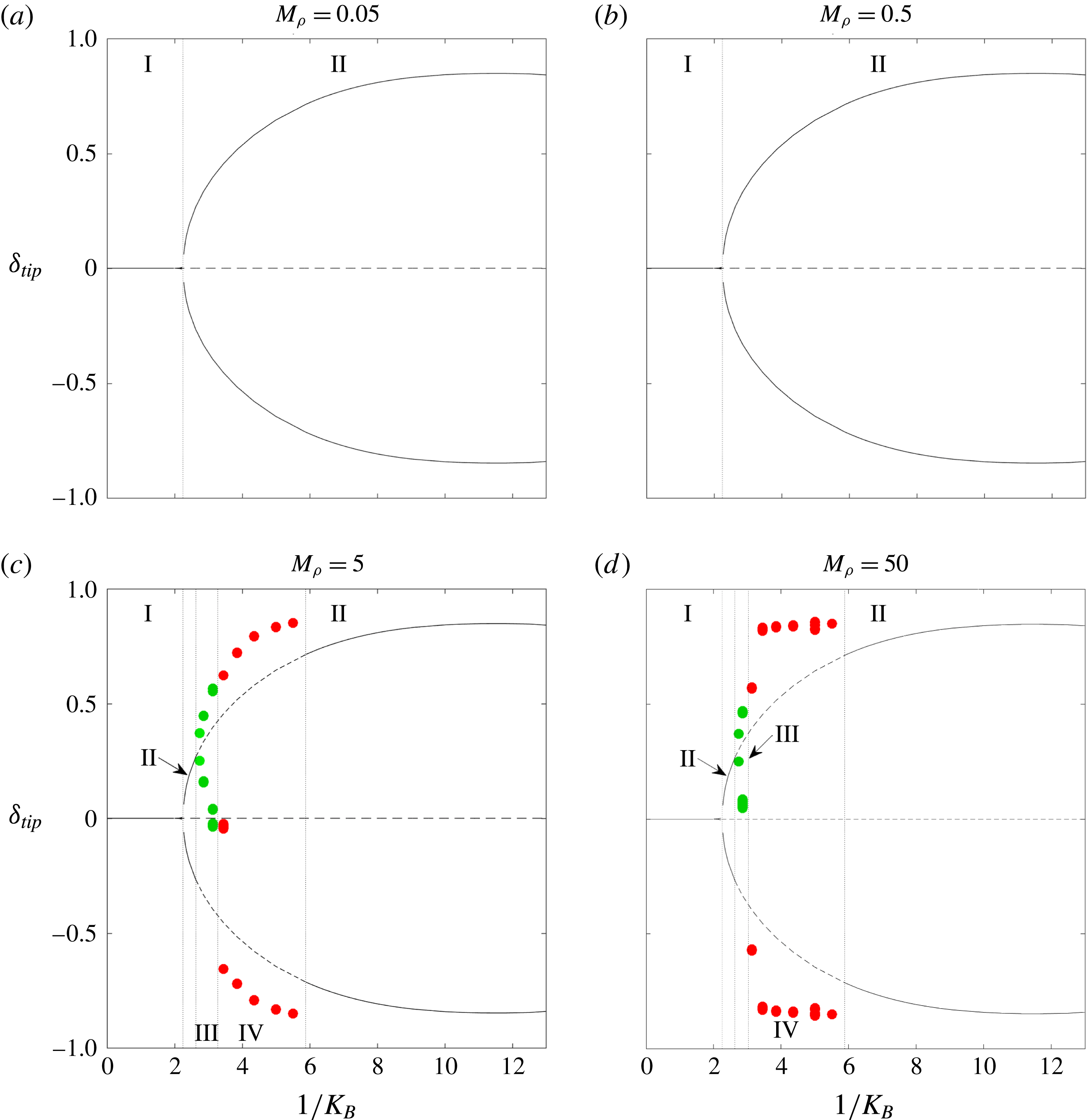
to investigate the stability and dynamics of the inverted-flag system below this previously identified critical Reynolds number. Figure 18 gives bifurcation diagrams of the inverted-flag system at four different mass ratios. These figures were plotted as described in § 3. As with
 $Re=200$
, a minimum of fifteen flapping cycles were used to convey flapping information on the diagrams. The bifurcation diagrams reveal four distinct regimes: a stable undeformed equilibrium (I), a stable deformed equilibrium (II), small-deflection flapping (III) and large-amplitude flapping (IV).
While many of the same bifurcations found at
 $Re=200$
remain for
 $Re=20$
, there are also distinctions between them that are visible through the bifurcation diagrams. First, consistent with the observations of Ryu et al. (Reference Ryu, Park, Kim and Sung2015) and Shoele & Mittal (Reference Shoele and Mittal2016), we do not find flapping for light flags (
 $M_{\unicode[STIX]{x1D70C}}\leqslant 0.5$
). This demonstrates the stabilising effect of viscosity for inverted-flag dynamics. However, heavy flags with
 $M_{\unicode[STIX]{x1D70C}}=5,50$
are found to undergo both small-deflection flapping and large-amplitude flapping. We discuss the mechanisms behind this flapping behaviour in subsequent sections. Second, the deflected-mode state no longer exhibits flapping at this lower Reynolds number, and is instead a true stable equilibrium of the fully coupled fluid–structure equations of motion. Finally, chaotic flapping does not occur for any of the considered values of
 $M_{\unicode[STIX]{x1D70C}}$
at this lower Reynolds number.
Bifurcation diagrams of inverted-flag dynamics at
 $Re=20$
that show leading-edge transverse displacement (tip deflection,
 $\unicode[STIX]{x1D6FF}_{tip}$
) versus inverse stiffness (
 $1/K_{B}$
). I, undeformed equilibrium; II, deformed equilibrium; III, small-deflection flapping; IV, large-amplitude flapping. See the main text for a description of the various lines and markers and details on how the diagrams were constructed.
As was seen for
 $Re=200$
, the divergence instability of the undeformed equilibrium (caused by decreasing
 $K_{B}$
) leads to a stable deformed equilibrium (region II in figure 18) that is independent of the mass ratio,
 $M_{\unicode[STIX]{x1D70C}}$
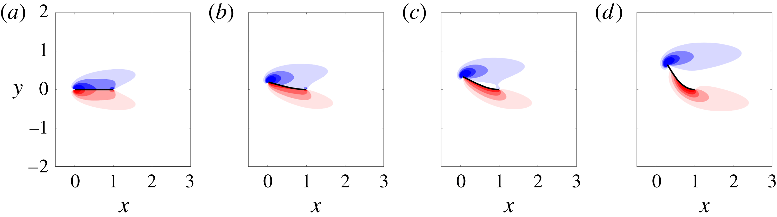
. This follows from the fact that the deformed equilibria are steady-state solutions and therefore do not depend on flag inertia. The deformed equilibria for
 $Re=20$
are shown in figure 19.
Vorticity contours for equilibrium states of the inverted-flag system at
 $Re=20$
. From (a) to (d),
 $K_{B}=0.5,0.41,0.35,0.2$
. The two rightmost equilibria are unstable for
 $M_{\unicode[STIX]{x1D70C}}=5,50$
. Contours are in 18 increments from
 $-$
5 to 5.
As stiffness is decreased, light flags remain in this (stable) deformed equilibrium regime: no flapping occurs at this Reynolds number for
 $M_{\unicode[STIX]{x1D70C}}=0.05,0.5$
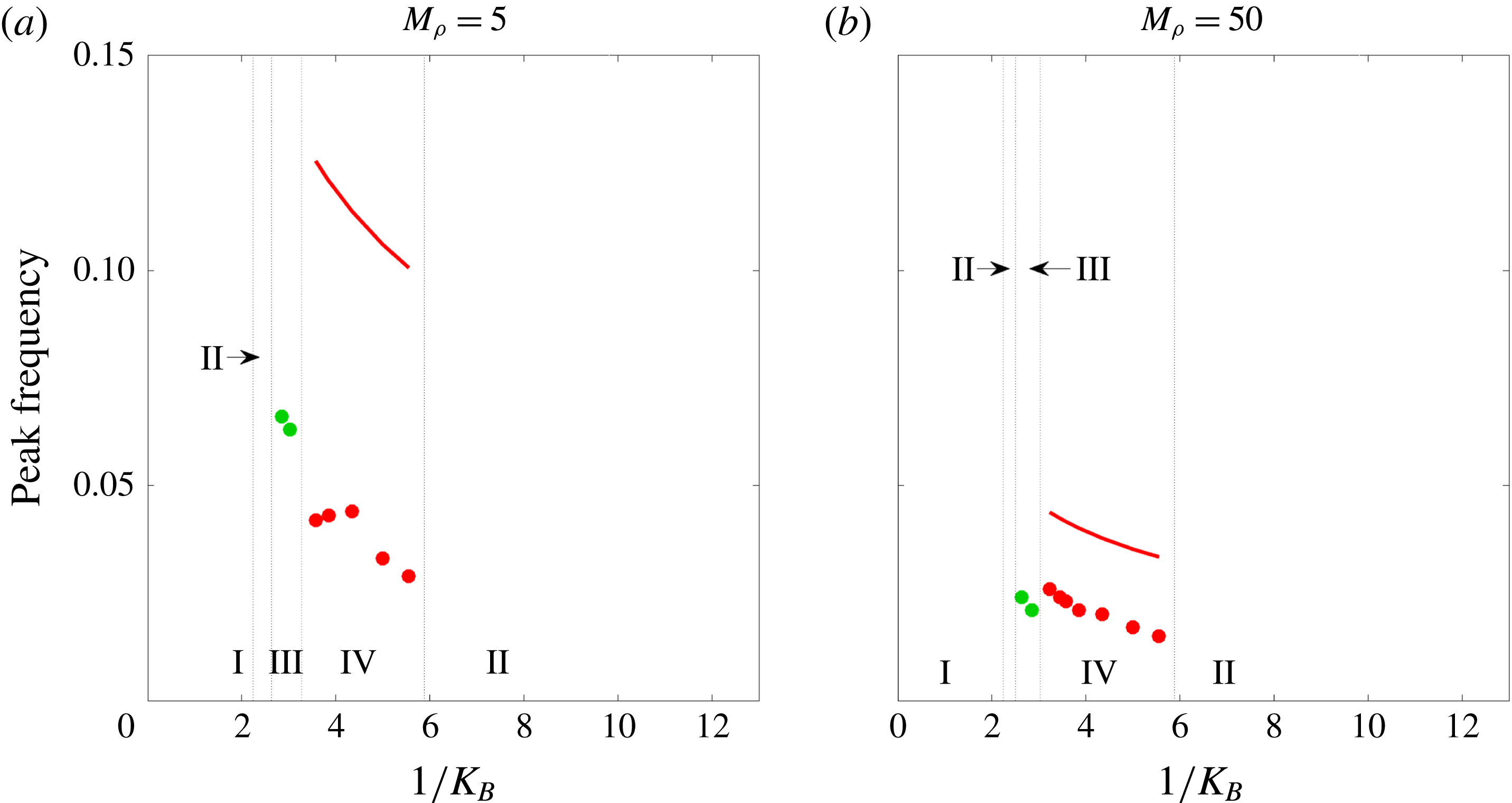
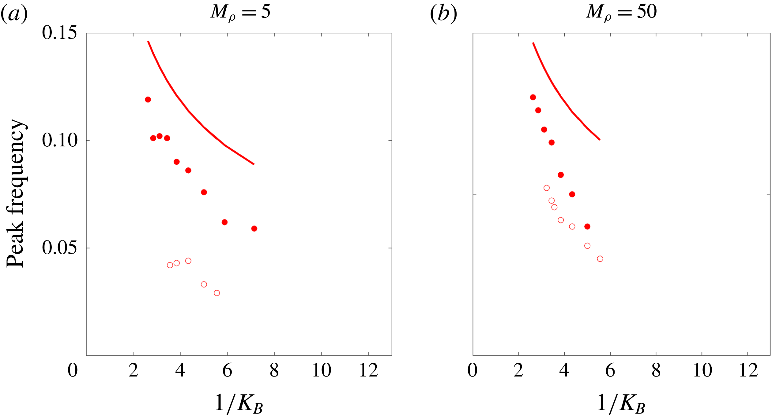
. Moreover, since the equilibrium states do not depend on flag inertia, their bifurcation diagrams are identical. By contrast, with decreasing stiffness heavy flags transition from the deformed equilibrium to (respectively) small-deflection flapping and large-amplitude flapping before returning at even lower stiffnesses to a stable deformed equilibrium; the amplitude jumps abruptly at this latter transition. We show in figure 20 the peak flapping frequency for the parameters corresponding to the bifurcation diagrams in figure 18. We will refer to this frequency figure in subsequent sections, as appropriate.
Markers: peak flapping frequency at
 $Re=20$
for the parameters corresponding to the bifurcation diagrams shown in figure 18; ——, natural frequency scaling of a sheet accounting for added mass contributions from an inviscid fluid, as derived in Shen et al. (Reference Shen, Chakraborty and Sader2016).
4.2 Small-deflection flapping
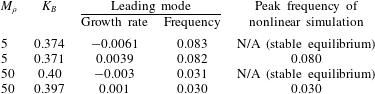
We show in table 6 that the transition from the (stable) deformed equilibrium to small-deflection flapping is associated with the least damped global mode of the deformed equilibrium becoming unstable. Thus, as was seen for
 $Re=200$
, small-deflection flapping is a supercritical Hopf bifurcation of the deformed-equilibrium state. Table 6 also shows that the corresponding eigenvalue accurately predicts the flapping frequency of the nonlinear simulations near the stability boundary. Note that flapping in this regime is not a classical VIV – the markers in region III of the frequency plots (figure 20) are significantly smaller than the expected value for vortex shedding of 0.2.
Growth rate and frequency of the leading global mode of the deformed equilibrium compared with nonlinear behaviour for parameters near the onset of small-deflection flapping.
To illustrate the vortical regions and flag shapes associated with this instability at this lower Reynolds number of
 $Re=20$
, we plot the real and imaginary parts of the leading global mode near the critical stiffness for
 $M_{\unicode[STIX]{x1D70C}}=5$
in figure 21 (the plot is similar for
 $M_{\unicode[STIX]{x1D70C}}=50$
). Flag motion is associated with four vortical structures near the flag surface.
Real (a,b) and imaginary (c,d) parts of vorticity (a,c) and flag displacement (b,d) of the leading global mode of the deformed equilibrium for
 $M_{\unicode[STIX]{x1D70C}}=5,K_{B}=0.37$
and
 $Re=20$
. Vorticity contours are in 20 increments from
 $-$
0.05 to 0.05.
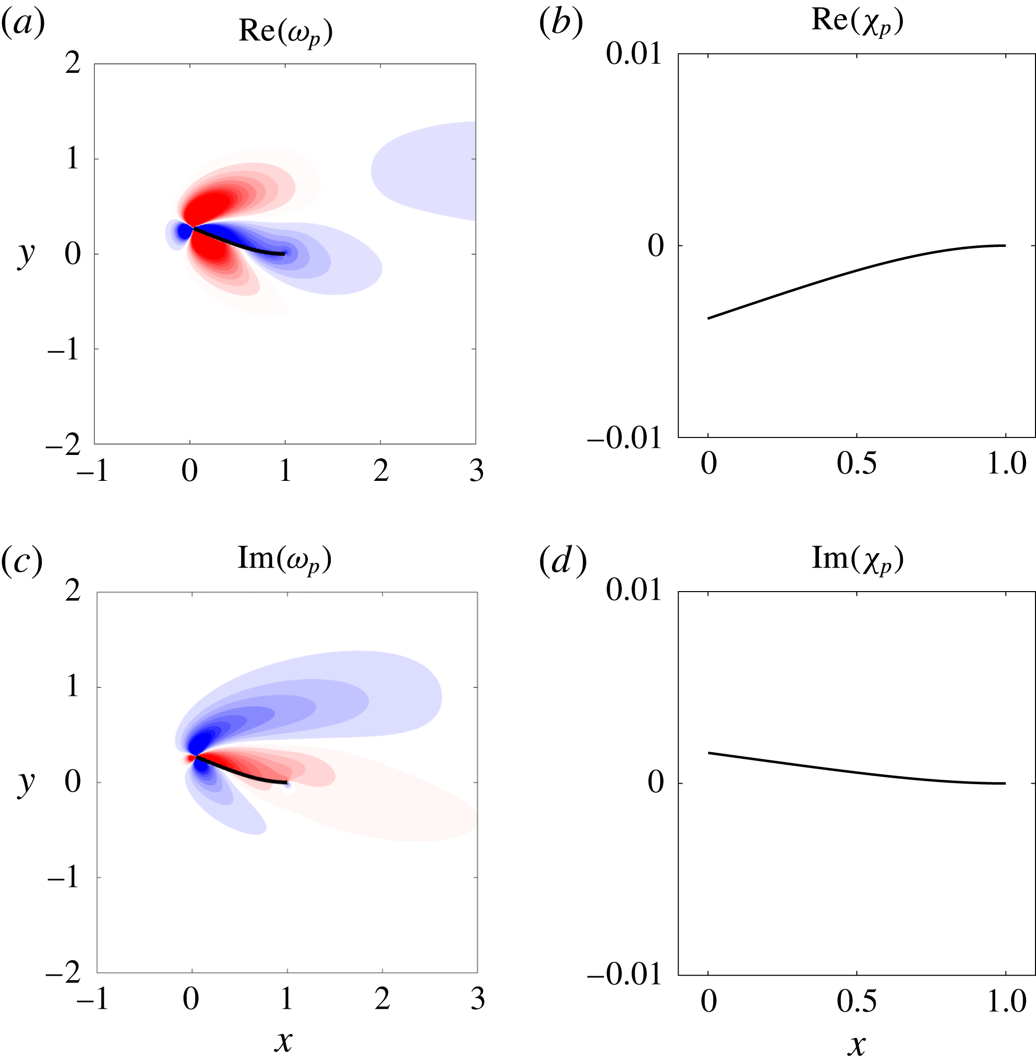
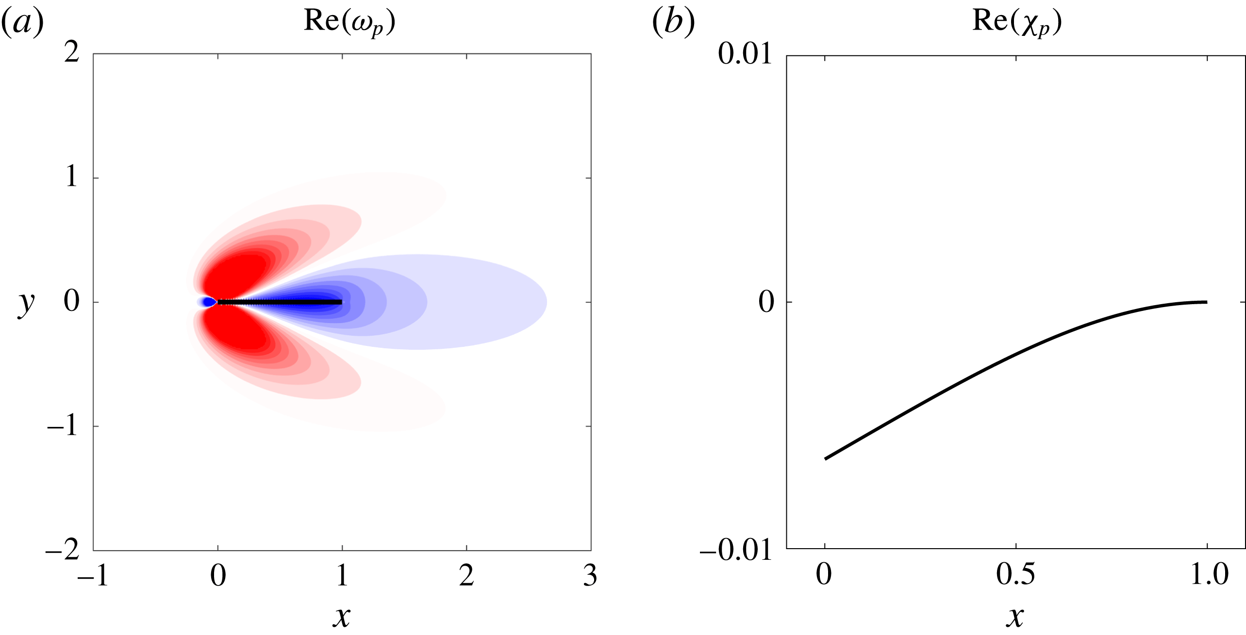
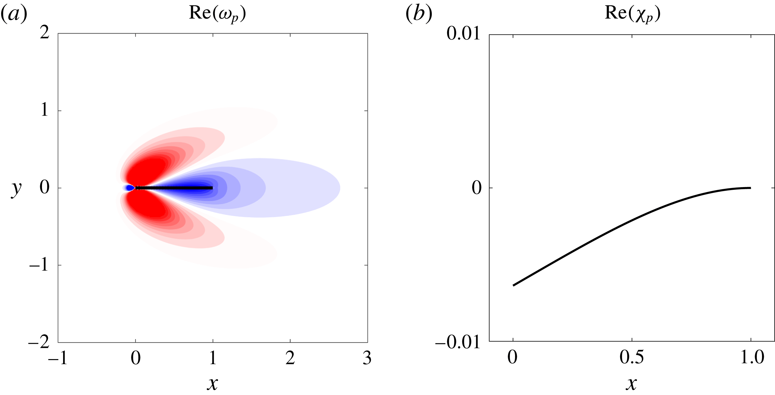
We emphasise that a linear stability analysis of the undeformed equilibrium state is associated with a zero-frequency (non-flapping) unstable mode; it is therefore distinct from the flapping behaviour observed in the nonlinear simulations. This establishes that the divergence instability derived by Sader et al. (Reference Sader, Cossé, Kim, Fan and Gharib2016a ) for inviscid fluids persists at lower Reynolds numbers. The undeformed-equilibrium state is unstable during flapping.
Figure 22 shows the leading global mode of the undeformed equilibrium (note that the leading mode of the undeformed equilibrium is purely real). The mode has a deflected flag shape and set of vortical structures that are similar to the real part of the leading mode of the deformed equilibrium. A noticeable distinction between the two, however, is that the vortical structures of the undeformed-equilibrium mode are symmetric about the equilibrium flag position while those of the deformed-equilibrium mode are not (and the latter occur at non-zero frequency).
Real part of vorticity (a) and flag displacement (b) of the leading global mode of the undeformed equilibrium for
 $M_{\unicode[STIX]{x1D70C}}=5,K_{B}=0.37$
and
 $Re=20$
. Vorticity contours are in 20 increments from
 $-$
0.05 to 0.05.
4.3 Large-amplitude flapping
We now consider the transition from small-deflection flapping to large-amplitude flapping. Large-amplitude flapping is observed only for large mass ratios at this smaller Reynolds number. We first explore the mechanism behind this observation.
At small mass ratios, unsteady inertia of the fluid dominates inertia in the flag. As such, the flow dynamics are not strongly perturbed by the flag. In contrast, at high mass ratios the fluid exerts a weak effect – the system dynamics are structure-dominated. This behaviour is borne out in figure 20, where the flapping frequency is comparable to that of the natural frequency of the flag (in an inviscid fluid). Note that there is a downward shift in the flapping frequency due to the effect of viscosity. This effect is expected (Sader Reference Sader1998), and is demonstrated further in figure 23: with increasing viscosity the effects of added mass are enhanced, and hence flapping frequency decreases.
Viscosity (shear stress) is known to stabilise vortex formation behind a bluff body. This leads to the extinction of periodic vortex shedding for
 $Re<47$
behind a rigid cylinder. However, motion of the structure can relax these stabilising shear stresses, leading to unsteadiness in vortex formation (and shedding) for
 $Re<47$
. This physics underlies the sub-critical VIV observed in elastic cylinders at high
 $M_{\unicode[STIX]{x1D70C}}$
(Mittal & Singh Reference Mittal and Singh2005), i.e. in the structure-dominated regime. Similarly, stabilising viscous stresses at low
 $Re$
are relaxed in the inverted-flag system, provided
 $M_{\unicode[STIX]{x1D70C}}$
is large. While vortex shedding is not observed in the inverted-flag system at this sub-critical Reynolds number (see figure 24), flapping ensues nonetheless. This suggests that vortex formation is again destabilised at high
 $M_{\unicode[STIX]{x1D70C}}$
and low
 $Re$
(as for sub-critical VIV of elastic cylinders), leading to vibration of the structure. In contrast to sub-critical VIV of elastic cylinders, however, the Strouhal number is much smaller than 0.2. This indicates that the natural frequency of unsteadiness in vorticity formation (due to flow convection) is much higher than the flag’s resonant frequency (which sets the vibration frequency at large
 $M_{\unicode[STIX]{x1D70C}}$
). This is identical to the observation for
 $Re=200$
at large
 $M_{\unicode[STIX]{x1D70C}}$
(see § 3.3.2), and can therefore be classified as not classical VIV.
Flapping frequency for various Reynolds numbers: ——, natural frequency of a flag in the inviscid limit accounting for added mass (obtained using the method of (Shen et al.
Reference Shen, Chakraborty and Sader2016)); filled markers, peak flapping frequency for
 $Re=200$
; open markers, peak flapping frequency for
 $Re=20$
.
Vorticity contours at four snapshots of a flapping period of a flag in large-amplitude flapping for
 $Re=20$
,
 $M_{\unicode[STIX]{x1D70C}}=5$
, and
 $K_{B}=0.26$
. Contours are in 18 increments from
 $-$
5 to 5.
4.4 Large-deflection equilibrium (deflected-mode regime)
A continued decrease in stiffness leads to a bifurcation from large-amplitude flapping back to a stable deformed equilibrium with large deflection. This transition corresponds to the re-stabilisation of the leading global mode (e.g. for
 $M_{\unicode[STIX]{x1D70C}}=5$
,
 $K_{B}=0.17$
the growth rate of the leading mode is
 $-$
0.032). Note that this deflected-mode state is distinct from that found at the higher Reynolds numbers,
 $Re=200$
, where the flag undergoes small-amplitude oscillations driven by vortex shedding (Sader et al.
Reference Sader, Cossé, Kim, Fan and Gharib2016a
; Shoele & Mittal Reference Shoele and Mittal2016). Since vortex shedding is absent at
 $Re=20$
, the deflected-mode regime is a formal equilibrium of the fully coupled equations of motion.
5 Conclusions
We used 2-D high-fidelity nonlinear simulations and a global linear stability analysis of inverted-flag flapping to (i) investigate the physical mechanisms responsible for the onset of flapping, (ii) study the role of vortex shedding in large-amplitude flapping and (iii) further characterise various regime bifurcations that were previously identified and explored (Kim et al.
Reference Kim, Cossé, Cerdeira and Gharib2013; Gurugubelli & Jaiman Reference Gurugubelli and Jaiman2015; Ryu et al.
Reference Ryu, Park, Kim and Sung2015; Shoele & Mittal Reference Shoele and Mittal2016; Sader et al.
Reference Sader, Cossé, Kim, Fan and Gharib2016a
; Gurugubelli & Jaiman Reference Gurugubelli and Jaiman2017). We performed studies at
 $Re=20$
and 200 for a wide range of
 $K_{B}$
and over a four orders of magnitude range of
 $M_{\unicode[STIX]{x1D70C}}$
. The following statics/dynamics of the inverted flag were observed with a systematic decrease in flag stiffness:
Deflected equilibrium above divergence. We demonstrated that for all mass ratios and Reynolds numbers considered, a stationary deflected state exists that is a formal equilibrium of the fully coupled equations. This deflected state persists as an unstable steady state even when flapping occurs. A similar deformed equilibrium was found at
 $Re=O(30\,000)$
by Sader et al. (Reference Sader, Cossé, Kim, Fan and Gharib2016a
) through the addition of damping; establishing similarities between these findings is an area for future work.
Small-deflection flapping. The deformed equilibrium becomes unstable and transitions to small-deflection flapping with decreasing stiffness (
 $K_{B}$
). This occurred at
 $Re=200$
for all mass ratios considered and at
 $Re=20$
for heavy flags (
 $M_{\unicode[STIX]{x1D70C}}>O(1)$
) only. This flapping transition was shown to be initiated by a supercritical Hopf bifurcation of the deformed-equilibrium state (i.e. a complex-conjugate set of eigenvectors becomes unstable). For all parameters that exhibited this small-deflection flapping regime, the leading mode and ensuing nonlinear behaviour appear to be devoid of vortex shedding and have a flapping frequency that is not commensurate with classical VIV behaviour; i.e. the Strouhal number is much smaller than 0.2.
Large-amplitude flapping. Light flags (
 $M_{\unicode[STIX]{x1D70C}}<O(1)$
) at
 $Re=200$
exhibit classical VIV behaviour in which vortex shedding and flag motion are synchronised at the same frequency. This coincides with the arguments of Sader et al. (Reference Sader, Cossé, Kim, Fan and Gharib2016a
) based on experimental measurements and a scaling analysis. As the stiffness
 $K_{B}$
is decreased, the natural frequency of the flag decreases below the natural vortex-shedding frequency, and disruption of classical VIV occurs. By contrast, heavy flags (
 $M_{\unicode[STIX]{x1D70C}}>O(1)$
) at
 $Re=200$
do not exhibit classical VIV behaviour – also consistent with the scaling analysis of Sader et al. (Reference Sader, Cossé, Kim, Fan and Gharib2016a
). Vortex shedding occurs at a higher frequency than the natural flag frequency. Strikingly, large-amplitude flapping also occurs for heavy flags at
 $Re=20$
, and (as with heavy flags at
 $Re=200$
) is not a classical VIV. This sub-critical behaviour is due to relaxation of (viscous) shear stresses in this structure-dominated regime (at high
 $M_{\unicode[STIX]{x1D70C}}$
), which then allows unsteadiness in vorticity generation to ensue. No flapping was observed for flags in the fluid-dominated regime of
 $M_{\unicode[STIX]{x1D70C}}<O(1)$
at
 $Re=20$
, in agreement with the simulations of Ryu et al. (Reference Ryu, Park, Kim and Sung2015) and Shoele & Mittal (Reference Shoele and Mittal2016).
Deflected mode. For
 $Re=200$
we used a global stability analysis to confirm the argument of Shoele & Mittal (Reference Shoele and Mittal2016) that this regime is driven by the canonical bluff-body wake instability. For all masses considered, the leading mode has vortical structures similar to the leading global mode found in canonical bluff bodies (Barkley Reference Barkley2006) and a flapping frequency commensurate with the
 $St\sim 0.2$
bluff-body scaling (Roshko Reference Roshko1954). We also showed that the deflected mode does not exhibit flapping at any mass ratio for
 $Re=20$
, and the system is instead in a stable large-deflection equilibrium state.
Chaotic flapping. We confirmed the existence of chaotic flapping for light flags at
 $Re=200$
and characterised its onset as the destabilisation of classical VIV in large-amplitude flapping of light flags. We also demonstrated that the chaotic attractor involves switching between the unstable large-amplitude and deflected-mode states. The experimental identification of chaotic flapping by Sader et al. (Reference Sader, Cossé, Kim, Fan and Gharib2016a
) at Reynolds numbers
 $O(10\,000)$
indicates that chaos is possible over a wide range of fluid inertia. No chaotic flapping was observed at
 $Re=200$
for
 $M_{\unicode[STIX]{x1D70C}}>O(1)$
or at
 $Re=20$
for any of the mass ratios considered.
Acknowledgements
A.G. and T.C. gratefully acknowledge the computing resources provided to them through the NSF XSEDE program, and funding from Robert Bosch LLC through the Bosch Energy Research Network Grant (grant number 07.23.CS.15) and from the AFOSR (grant number FA9550-14-1-0328). J.E.S. thanks the ARC Centre of Excellence in Exciton Science and the Australian Research Council Grants Scheme.
Appendix A. Details of the global stability solver
We provide here more details for how the eigenvalue problem associated with (2.9) and (2.10) is solved. The matrices
 $\unicode[STIX]{x1D63C}$
and
 $\unicode[STIX]{x1D63D}$
are built and stored sparsely and solved using the built-in eigs command in MATLAB, which performs an implementation of the implicitly restarted Arnoldi algorithm (Lehoucq et al.
Reference Lehoucq, Sorensen and Yang1998). We focus here on the construction of submatrices
 $\unicode[STIX]{x1D645}^{\unicode[STIX]{x1D712}s}$
,
 $\unicode[STIX]{x1D645}^{\unicode[STIX]{x1D712}\unicode[STIX]{x1D712}}$
and
 $\unicode[STIX]{x1D645}^{\unicode[STIX]{x1D712}c}$
. All other submatrices of
 $\unicode[STIX]{x1D63C}$
and
 $\unicode[STIX]{x1D63D}$
are described in Goza & Colonius (Reference Goza and Colonius2017), and the reader is referred to that article for more details.
We describe
 $\unicode[STIX]{x1D645}^{\unicode[STIX]{x1D712}s}$
in detail below; the formation of
 $\unicode[STIX]{x1D645}^{\unicode[STIX]{x1D712}\unicode[STIX]{x1D712}}$
and
 $\unicode[STIX]{x1D645}^{\unicode[STIX]{x1D712}c}$
are analogous. The primary challenge in constructing
 $\unicode[STIX]{x1D645}^{\unicode[STIX]{x1D712}s}$
lies in the fact that the
 $\unicode[STIX]{x2202}\unicode[STIX]{x1D60C}_{jl}^{\text{T}}/\unicode[STIX]{x2202}\unicode[STIX]{x1D712}_{k}$
term corresponds to a third-rank tensor. This third-rank tensor need not be built directly, however, as the
 $k$
th column of
 $\unicode[STIX]{x1D645}^{\unicode[STIX]{x1D712}s}$
is
 $$\begin{eqnarray}\displaystyle \unicode[STIX]{x1D63E}^{\text{T}}\frac{\unicode[STIX]{x2202}\unicode[STIX]{x1D640}}{\unicode[STIX]{x2202}\unicode[STIX]{x1D712}_{k}}\boldsymbol{f}_{b}. & & \displaystyle\end{eqnarray}$$
We moreover approximated the
 $\unicode[STIX]{x2202}\unicode[STIX]{x1D640}/\unicode[STIX]{x2202}\unicode[STIX]{x1D712}_{k}$
term with a first-order finite difference scheme in this work (note that this is consistent with the overall accuracy of the numerical method), so that
 $\unicode[STIX]{x1D645}^{\unicode[STIX]{x1D712}s}$
may be constructed columnwise, with the
 $k$
th column computed as
 $$\begin{eqnarray}\displaystyle \unicode[STIX]{x1D63E}^{\text{T}}\left[\frac{\unicode[STIX]{x1D640}^{\text{T}}(\unicode[STIX]{x1D74C}_{b}+\unicode[STIX]{x1D716}\boldsymbol{e}_{k})-\unicode[STIX]{x1D640}^{\text{T}}(\unicode[STIX]{x1D74C}_{b})}{\unicode[STIX]{x1D716}}\right]\boldsymbol{f}_{b}, & & \displaystyle\end{eqnarray}$$
where
 $\boldsymbol{e}_{k}$
is the
 $k$
th unit vector with zero values in all entries except for the
 $k$
th, and
 $\unicode[STIX]{x1D716}$
is a real scalar with
 $\unicode[STIX]{x1D716}\ll 1$
. We used
 $\unicode[STIX]{x1D716}=10^{-5}$
in our studies, but noticed negligible differences in the results for
 $10^{-6}\leqslant \unicode[STIX]{x1D716}\leqslant 10^{-3}$
.
Appendix B. Grid convergence study
We give here the details of a grid convergence study of the nonlinear solver for
 $Re=200,M_{\unicode[STIX]{x1D70C}}=0.5,K_{B}=0.35$
. For these parameters the flag enters limit-cycle flapping of fixed amplitude and frequency. The details of the grid spacing on the finest sub-domain (
 $\unicode[STIX]{x0394}x$
), time step (
 $\unicode[STIX]{x0394}t$
), smallest sub-domain size and total domain size are provided in table 7. In all cases, the grid spacing on the flag was set to be twice that of the grid spacing on the finest domain.
Parameters used for grid-convergence study.
 $\unicode[STIX]{x0394}x$
, grid spacing on finest sub-domain;
 $\unicode[STIX]{x0394}t$
, time step. Grid 3 was used to obtain the results presented throughout the manuscript.

Grid 4 was used as the fine-grid solution to determine grid convergence. Figure 25 shows the normalised
 $L_{\infty }$
-norm of the discrepancy in the flag displacement between the coarse- and fine-grid solutions at
 $t=5$
(i.e.
 $\unicode[STIX]{x1D716}_{h}\equiv \Vert \unicode[STIX]{x1D74C}_{h}-\unicode[STIX]{x1D74C}_{f}\Vert _{\infty }/\Vert \unicode[STIX]{x1D74C}_{f}\Vert _{\infty }$
, where
 $\unicode[STIX]{x1D74C}_{f}$
and
 $\unicode[STIX]{x1D74C}_{h}$
denote the flag displacement computed with the fine and coarse grids, respectively). The plot illustrates the expected first-order convergence rate and demonstrates the good agreement between the solutions obtained with grids 3 and 4. To further indicate the grid-converged nature of the results, we show in table 8 the peak amplitude and frequency associated with the limit-cycle behaviour, as computed using grids 1–4. Note that even grid 1 yields a fairly accurate representation of the time-averaged behaviour of the system.
Normalised
 $L_{\infty }$
-norm of the discrepancy in the flag displacement between the coarse- and fine-grid solutions at
 $t=5$
(
 $x$
): - - -, first-order convergence rate.
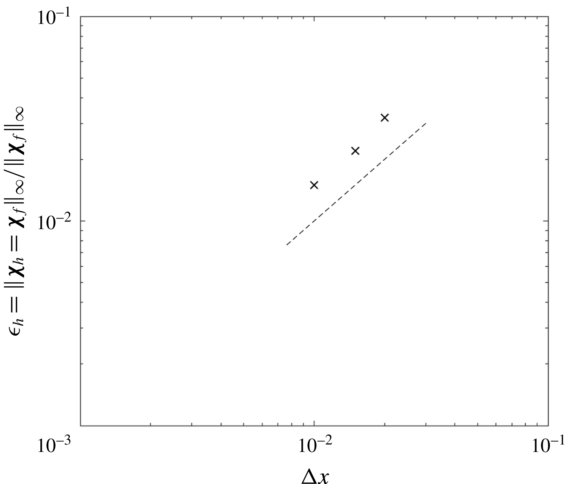
Peak amplitude and flapping frequency associated with limit-cycle flapping of an inverted flag for
 $Re=200,M_{\unicode[STIX]{x1D70C}}=0.5,$
and
 $K_{B}=0.35$
, as obtained using grids 1–4.
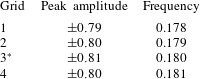
The immersed-boundary method of Goza & Colonius (Reference Goza and Colonius2017) used in this work intrinsically satisfies the no-slip boundary at each point along the flag to within a prescribed tolerance (e.g. the slip magnitude at each discrete flag point was less than
 $10^{-9}$
in all simulations).
An illustration that describes the steps used to populate the markers at
 $1/K_{B}\approx 6$
for the
 $M_{\unicode[STIX]{x1D70C}}=0.05$
,
 $Re=200$
bifurcation diagram.
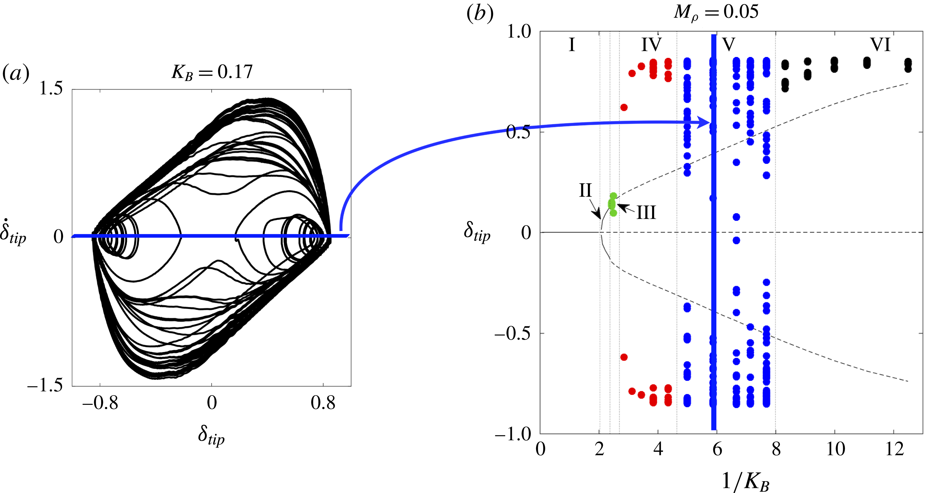
Appendix C. Building bifurcation diagrams
For clarity, we describe further how the set of markers corresponding to
 $1/K_{B}\approx 6$
was obtained for the
 $Re=200$
,
 $M_{\unicode[STIX]{x1D70C}}=0.05$
bifurcation diagram. This discussion is facilitated through figure 26. From a simulation for
 $Re=200$
,
 $M_{\unicode[STIX]{x1D70C}}=0.05$
, and
 $1/K_{B}\approx 6$
, a phase portrait (figure 26
a) of tip velocity (
 $\dot{\unicode[STIX]{x1D6FF}}_{tip}$
) versus tip displacement (
 $\unicode[STIX]{x1D6FF}_{tip}$
) was constructed based off of time traces of those quantities. Note that initial transients were removed, and the phase portrait was obtained using only information after the first five flapping cycles. A zero-tip-velocity Poincaré section was then obtained by taking a horizontal cross-section of the curve in figure 26(a). The points of the phase portrait that intersect this zero-velocity slice were then used to populate the bifurcation diagram at
 $1/K_{B}\approx 6$
. This procedure was repeated at all other values of
 $1/K_{B}$
for which there are markers.