2.1 Governing equations

Consider the probability density function $P$ of active particles in the position–orientation space $(\boldsymbol{R}^{\ast },\boldsymbol{p})$ , where $\boldsymbol{R}^{\ast }$ is the position and $\boldsymbol{p}$ is the orientation. We have the probability flux conservation equation, i.e. the Smoluchowski equation (Doi & Edwards Reference Doi and Edwards1988), as

(2.1) $$\begin{eqnarray}{\displaystyle \frac{\unicode[STIX]{x2202}P}{\unicode[STIX]{x2202}t^{\ast }}}+\unicode[STIX]{x1D735}_{R}^{\ast }\boldsymbol{\cdot }\boldsymbol{J}_{R}^{\ast }+\unicode[STIX]{x1D735}_{p}\boldsymbol{\cdot }\boldsymbol{J}_{p}^{\ast }=0,\end{eqnarray}$$

where $\unicode[STIX]{x1D735}_{R}^{\ast }$ denotes the gradient operator in the position space, $\unicode[STIX]{x1D735}_{p}$ is in the swimming orientation space, $t^{\ast }$ is the time,

(2.2) $$\begin{eqnarray}\boldsymbol{J}_{R}^{\ast }=[\boldsymbol{U}^{\ast }(\boldsymbol{R}^{\ast })+V_{s}^{\ast }\boldsymbol{p}]P-D_{t}^{\ast }\unicode[STIX]{x1D735}_{R}^{\ast }P,\end{eqnarray}$$

is the position-space flux density and

(2.3) $$\begin{eqnarray}\boldsymbol{J}_{p}^{\ast }=\dot{\boldsymbol{p}}^{\ast }P-D_{r}^{\ast }\unicode[STIX]{x1D735}_{p}P,\end{eqnarray}$$

is the orientation-space flux density, with $\boldsymbol{U}^{\ast }$ standing for the velocity of the external flow, $V_{s}^{\ast }$ the mean swimming speed of the particles, $D_{t}^{\ast }$ the translational diffusivity and $D_{r}^{\ast }$ the rotational diffusivity. The rate of change of swimming direction (Leal & Hinch Reference Leal and Hinch1972; Pedley & Kessler Reference Pedley and Kessler1992) is given by

(2.4) $$\begin{eqnarray}\dot{\boldsymbol{p}}^{\ast }={\textstyle \frac{1}{2}}\unicode[STIX]{x1D74E}^{\ast }\wedge \boldsymbol{p}+\unicode[STIX]{x1D6FC}_{0}\boldsymbol{p}\boldsymbol{\cdot }\unicode[STIX]{x1D640}^{\ast }\boldsymbol{\cdot }(\unicode[STIX]{x1D644}-\boldsymbol{p}\boldsymbol{p}),\end{eqnarray}$$

where a dot above a variable denotes the time derivative, $\unicode[STIX]{x1D74E}^{\ast }$ is the ambient vorticity

(2.5) $$\begin{eqnarray}\unicode[STIX]{x1D74E}^{\ast }=\unicode[STIX]{x1D735}_{R}^{\ast }\wedge \boldsymbol{U}^{\ast },\end{eqnarray}$$

$\unicode[STIX]{x1D640}^{\ast }$ is the rate-of-strain tensor

(2.6) $$\begin{eqnarray}\unicode[STIX]{x1D640}^{\ast }={\textstyle \frac{1}{2}}[\unicode[STIX]{x1D735}_{R}^{\ast }\boldsymbol{U}^{\ast }+(\unicode[STIX]{x1D735}_{R}^{\ast }\boldsymbol{U}^{\ast })^{\text{T}}],\end{eqnarray}$$

$\unicode[STIX]{x1D644}$ is the identity tensor, $\unicode[STIX]{x1D6FC}_{0}$ is the shape factor of the particle, with $\unicode[STIX]{x1D6FC}_{0}=0$ for a spherical particle and $\unicode[STIX]{x1D6FC}_{0}=1$ for an infinitely thin rod-like particle.

Figure 1.

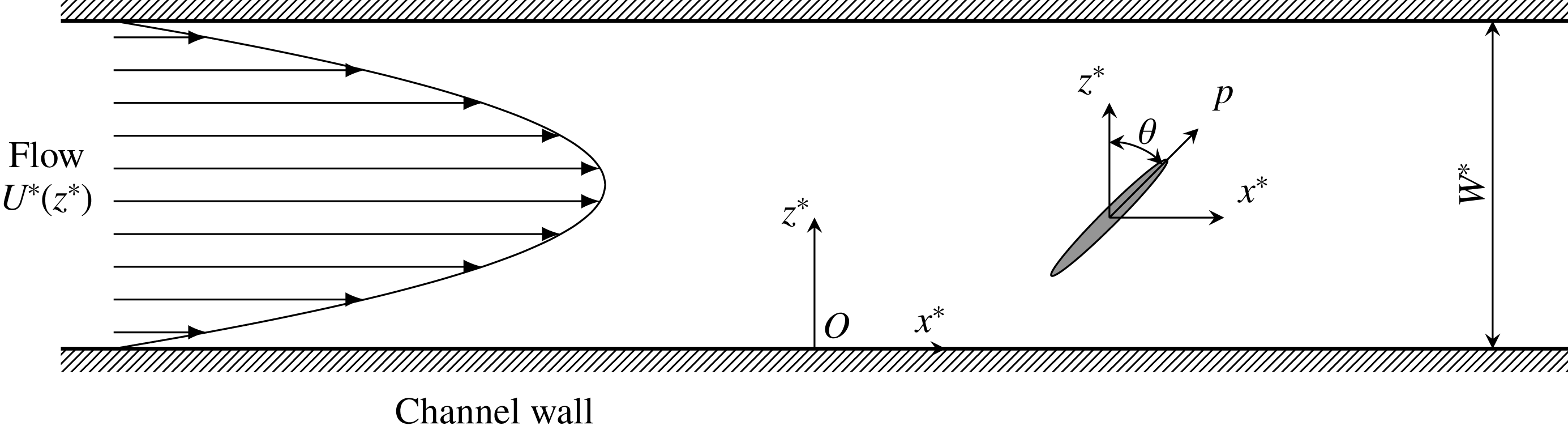
Sketch of a dilute suspension of active particles in a confined unidirectional flow.

For a dilute suspension of active particles in a unidirectional flow confined by a channel of width $W^{\ast }$ , as depicted in figure 1 with $\boldsymbol{R}^{\ast }=(x^{\ast },z^{\ast })$ and $\boldsymbol{p}=(\sin \unicode[STIX]{x1D703},\cos \unicode[STIX]{x1D703})$ , the flow velocity is

(2.7) $$\begin{eqnarray}\boldsymbol{U}^{\ast }(\boldsymbol{R}^{\ast })=(U^{\ast }(z^{\ast }),0).\end{eqnarray}$$

Then the velocity gradient tensor is

(2.8) $$\begin{eqnarray}\unicode[STIX]{x1D735}_{R}^{\ast }\boldsymbol{U}^{\ast }=\left(\begin{array}{@{}cc@{}}0 & 0\\[3.0pt] S(z^{\ast }) & 0\end{array}\right),\end{eqnarray}$$

where

(2.9) $$\begin{eqnarray}S^{\ast }(z^{\ast })={\displaystyle \frac{\text{d}U^{\ast }}{\text{d}z^{\ast }}}.\end{eqnarray}$$

For the angular velocity

(2.10) $$\begin{eqnarray}\unicode[STIX]{x1D6FA}^{\ast }(z^{\ast },\unicode[STIX]{x1D703})=\dot{\boldsymbol{p}}^{\ast }\boldsymbol{\cdot }\boldsymbol{e}_{\unicode[STIX]{x1D703}},\end{eqnarray}$$

where $\boldsymbol{e}_{\unicode[STIX]{x1D703}}$ is the unit vector perpendicular to the swimming direction $\boldsymbol{p}$ , an explicit expression is

(2.11) $$\begin{eqnarray}\unicode[STIX]{x1D6FA}^{\ast }(z^{\ast },\unicode[STIX]{x1D703})={\displaystyle \frac{S^{\ast }(z^{\ast })}{2}}+\unicode[STIX]{x1D6FC}_{0}{\displaystyle \frac{S^{\ast }(z^{\ast })}{2}}(2\cos ^{2}\unicode[STIX]{x1D703}-1).\end{eqnarray}$$

The probability flux conservation equation (2.1) becomes

(2.12) $$\begin{eqnarray}\displaystyle & & \displaystyle {\displaystyle \frac{\unicode[STIX]{x2202}P}{\unicode[STIX]{x2202}t^{\ast }}}+[U^{\ast }(z^{\ast })+V_{s}^{\ast }\sin \unicode[STIX]{x1D703}]{\displaystyle \frac{\unicode[STIX]{x2202}P}{\unicode[STIX]{x2202}x^{\ast }}}+V_{s}^{\ast }\cos \unicode[STIX]{x1D703}{\displaystyle \frac{\unicode[STIX]{x2202}P}{\unicode[STIX]{x2202}z^{\ast }}}+{\displaystyle \frac{\unicode[STIX]{x2202}}{\unicode[STIX]{x2202}\unicode[STIX]{x1D703}}}\left[\unicode[STIX]{x1D6FA}^{\ast }(z^{\ast },\unicode[STIX]{x1D703})P-D_{r}^{\ast }{\displaystyle \frac{\unicode[STIX]{x2202}P}{\unicode[STIX]{x2202}\unicode[STIX]{x1D703}}}\right]\nonumber\\ \displaystyle & & \displaystyle \qquad =D_{t}^{\ast }{\displaystyle \frac{\unicode[STIX]{x2202}^{2}P}{\unicode[STIX]{x2202}x^{\ast 2}}}+D_{t}^{\ast }{\displaystyle \frac{\unicode[STIX]{x2202}^{2}P}{\unicode[STIX]{x2202}z^{\ast 2}}}.\end{eqnarray}$$

2.2 Solid boundary conditions

To account for the wall accumulation of the confined active suspension, the Robin boundary condition (Ezhilan & Saintillan Reference Ezhilan and Saintillan2015) is introduced as

(2.13) $$\begin{eqnarray}D_{t}^{\ast }{\displaystyle \frac{\unicode[STIX]{x2202}P}{\unicode[STIX]{x2202}z^{\ast }}}=V_{s}^{\ast }\cos \unicode[STIX]{x1D703}P,\quad \text{at }z^{\ast }=0,W^{\ast },\end{eqnarray}$$

with no penetration of the probability flux at the walls, as the wall-normal swimming flux and the translational diffusion flux are balanced (Ezhilan & Saintillan Reference Ezhilan and Saintillan2015). Thus, the particles swimming towards a wall must be balanced by a positive wall-normal gradient. Conversely, the particles swimming away from a wall will lead to a negative gradient. The conservation of particles near walls prefers a net polarization towards the wall, which leads to the wall accumulation (Ezhilan & Saintillan Reference Ezhilan and Saintillan2015). Note that this mechanism of accumulation does not include the hydrodynamic interactions among the particles, the wall and the flow.

Equally typical, the reflection condition for the swimming flux (Bearon et al. Reference Bearon, Hazel and Thorn2011; Ezhilan et al. Reference Ezhilan, Pahlavan and Saintillan2012; Ezhilan & Saintillan Reference Ezhilan and Saintillan2015)

(2.14) $$\begin{eqnarray}P(x^{\ast },z^{\ast },\unicode[STIX]{x1D703},t^{\ast })=P(x^{\ast },z^{\ast },\unicode[STIX]{x03C0}-\unicode[STIX]{x1D703},t^{\ast }),\quad \text{at }z^{\ast }=0,W^{\ast },\end{eqnarray}$$

is also imposed at solid boundaries due to their perfectly elastic collisions with the active particles.

Actually, there are various forms of boundary conditions to ensure the conservation of particles. Several studies (Ezhilan et al. Reference Ezhilan, Pahlavan and Saintillan2012; Bearon & Hazel Reference Bearon and Hazel2015) imposed a weaker condition as

(2.15) $$\begin{eqnarray}\int _{0}^{2\unicode[STIX]{x03C0}}D_{t}^{\ast }{\displaystyle \frac{\unicode[STIX]{x2202}P}{\unicode[STIX]{x2202}z^{\ast }}}-V_{s}^{\ast }\cos \unicode[STIX]{x1D703}P\;\text{d}\unicode[STIX]{x1D703}=0,\quad \text{at}\,z^{\ast }=0,W^{\ast },\end{eqnarray}$$

i.e. zero total wall-normal probability flux at the walls. While both Robin and reflection conditions can satisfy the integral condition (2.15), the latter is insufficient to obtain a unique solution for (2.12), as discussed in Bearon & Hazel (Reference Bearon and Hazel2015) and Ezhilan & Saintillan (Reference Ezhilan and Saintillan2015).

2.3 Dimensionless formulation

Introduce dimensionless variables and parameters as

(2.16) $$\begin{eqnarray}\left.\begin{array}{@{}c@{}}t=t^{\ast }D_{r}^{\ast },\quad x={\displaystyle \frac{x^{\ast }}{W^{\ast }}}\quad z={\displaystyle \frac{z^{\ast }}{W^{\ast }}},\quad U={\displaystyle \frac{U^{\ast }}{U_{m}^{\ast }}},\quad \unicode[STIX]{x1D6FA}={\displaystyle \frac{\unicode[STIX]{x1D6FA}^{\ast }}{D_{r}^{\ast }}},\\ \mathit{Pe}_{s}={\displaystyle \frac{V_{s}^{\ast }}{D_{r}^{\ast }W^{\ast }}},\quad \mathit{Pe}_{f}={\displaystyle \frac{U_{m}^{\ast }}{D_{r}^{\ast }W^{\ast }}},\quad \unicode[STIX]{x1D6EC}={\displaystyle \frac{D_{t}^{\ast }}{V_{s}^{\ast 2}/D_{r}^{\ast }}},\end{array}\right\}\end{eqnarray}$$

where $U_{m}^{\ast }$ is the transverse mean velocity

(2.17) $$\begin{eqnarray}U_{m}^{\ast }\triangleq {\displaystyle \frac{1}{W^{\ast }}}\int _{0}^{W^{\ast }}U^{\ast }(z^{\ast })\;\text{d}z^{\ast },\end{eqnarray}$$

$\mathit{Pe}_{s}$ is the swimming Péclet number, indicating the ratio of the time that the swimmer takes to rotate entirely in the orientation space to the time that it takes to swim across the channel width; $\mathit{Pe}_{f}$ is the flow Péclet number, which quantifies the relative importance of the rotational diffusion to the alignment by the imposed shear flow; and $\unicode[STIX]{x1D6EC}$ is the ratio of the translational diffusivities ( $D_{t}^{\ast }$ ) to the translation of the particles generated by swimming ( $V_{s}^{\ast 2}/D_{r}^{\ast }$ ).

The transport equation (2.12) becomes

(2.18) $$\begin{eqnarray}{\displaystyle \frac{\unicode[STIX]{x2202}P}{\unicode[STIX]{x2202}t}}+[\mathit{Pe}_{f}U(z)+\mathit{Pe}_{s}\sin \unicode[STIX]{x1D703}]{\displaystyle \frac{\unicode[STIX]{x2202}P}{\unicode[STIX]{x2202}x}}-\unicode[STIX]{x1D6EC}\mathit{Pe}_{s}^{2}{\displaystyle \frac{\unicode[STIX]{x2202}^{2}P}{\unicode[STIX]{x2202}x^{2}}}+{\mathcal{L}}P=0,\end{eqnarray}$$

where

(2.19) $$\begin{eqnarray}{\mathcal{L}}(\boldsymbol{\cdot })\triangleq \mathit{Pe}_{s}\cos \unicode[STIX]{x1D703}{\displaystyle \frac{\unicode[STIX]{x2202}}{\unicode[STIX]{x2202}z}}(\boldsymbol{\cdot })+{\displaystyle \frac{\unicode[STIX]{x2202}}{\unicode[STIX]{x2202}\unicode[STIX]{x1D703}}}\left[\unicode[STIX]{x1D6FA}(z,\unicode[STIX]{x1D703})(\boldsymbol{\cdot })-{\displaystyle \frac{\unicode[STIX]{x2202}}{\unicode[STIX]{x2202}\unicode[STIX]{x1D703}}}(\boldsymbol{\cdot })\right]-\unicode[STIX]{x1D6EC}\mathit{Pe}_{s}^{2}{\displaystyle \frac{\unicode[STIX]{x2202}^{2}}{\unicode[STIX]{x2202}z^{2}}}(\boldsymbol{\cdot }),\end{eqnarray}$$

is an operator corresponding to the transport in the local section $Oz\unicode[STIX]{x1D703}$ .

The Robin boundary condition (2.13) is slightly modified as

(2.20) $$\begin{eqnarray}{\displaystyle \frac{\unicode[STIX]{x2202}P}{\unicode[STIX]{x2202}z}}={\displaystyle \frac{1}{\unicode[STIX]{x1D6EC}\mathit{Pe}_{s}}}\cos \unicode[STIX]{x1D703}P,\quad \text{at }z=0,1,\end{eqnarray}$$

and the reflection boundary condition (2.14) remains as

(2.21) $$\begin{eqnarray}P(x,z,\unicode[STIX]{x1D703},t)=P(x,z,\unicode[STIX]{x03C0}-\unicode[STIX]{x1D703},t),\quad \text{at }z=0,1.\end{eqnarray}$$

In the orientation dimension, periodic boundary conditions read as

(2.22) $$\begin{eqnarray}\displaystyle & \displaystyle P|_{\unicode[STIX]{x1D703}=0}=P|_{\unicode[STIX]{x1D703}=2\unicode[STIX]{x03C0}}, & \displaystyle\end{eqnarray}$$

(2.23) $$\begin{eqnarray}\displaystyle & \displaystyle \left.{\displaystyle \frac{\unicode[STIX]{x2202}P}{\unicode[STIX]{x2202}\unicode[STIX]{x1D703}}}\right|_{\unicode[STIX]{x1D703}=0}=\left.{\displaystyle \frac{\unicode[STIX]{x2202}P}{\unicode[STIX]{x2202}\unicode[STIX]{x1D703}}}\right|_{\unicode[STIX]{x1D703}=2\unicode[STIX]{x03C0}}. & \displaystyle\end{eqnarray}$$

An initial condition is prescribed

(2.24) $$\begin{eqnarray}P|_{t=0}=P^{(0)}(x,z,\unicode[STIX]{x1D703}),\end{eqnarray}$$

where $P^{(0)}$ is a probability distribution.

3.1 Local and global spaces

For a confined flow, the longitudinal scale is always much larger than the transverse scale. With a long enough longitudinal scale, because the time scale that the swimmer takes to rotate entirely in the orientation space is less than the scale it takes to swim in the main stream, the GTD theory can be effectively applied without any limit to the swimming Péclet number, as mentioned above. In this regard, the longitudinal coordinate $x$ is unbounded, and so qualifies the global-space coordinate variable $\boldsymbol{Q}=(x)$ . The local space is set as $\boldsymbol{q}=(z,\unicode[STIX]{x1D703})$ , since both the transverse coordinate $z$ and the orientation coordinate $\unicode[STIX]{x1D703}$ are bounded. The local space $\boldsymbol{q}$ can be interpreted as a cross-section $Oz\unicode[STIX]{x1D703}$ in the phase space (position–orientation space). Such a choice of local space enables one to characterize the transport problem of active particles by a one-dimensional macrotransport model, in contrast to the two-dimensional effective transport equation resulting from setting only the orientation space as the local space (Bearon et al. Reference Bearon, Hazel and Thorn2011).

Let $\boldsymbol{Q}\oplus \boldsymbol{q}$ denote the whole position–orientation space. We can redefine the flux density in the framework of the GTD theory as a global-space flux density $\boldsymbol{J}$ of

(3.1) $$\begin{eqnarray}\boldsymbol{J}=\left([\mathit{Pe}_{f}U(z)+\mathit{Pe}_{s}\sin \unicode[STIX]{x1D703}]P-\unicode[STIX]{x1D6EC}\mathit{Pe}_{s}^{2}{\displaystyle \frac{\unicode[STIX]{x2202}P}{\unicode[STIX]{x2202}x}}\right),\end{eqnarray}$$

and a local-space flux density $\boldsymbol{j}$ of

(3.2) $$\begin{eqnarray}\boldsymbol{j}=\left(\mathit{Pe}_{s}\cos \unicode[STIX]{x1D703}P-\unicode[STIX]{x1D6EC}\mathit{Pe}_{s}^{2}{\displaystyle \frac{\unicode[STIX]{x2202}P}{\unicode[STIX]{x2202}z}},\,\unicode[STIX]{x1D6FA}(z,\unicode[STIX]{x1D703})P-{\displaystyle \frac{\unicode[STIX]{x2202}P}{\unicode[STIX]{x2202}\unicode[STIX]{x1D703}}}\right).\end{eqnarray}$$

Then using the notation of vector gradient operators in $\boldsymbol{Q}$ - and $\boldsymbol{q}$ -space, the governing equation (2.18) is recast as

(3.3) $$\begin{eqnarray}{\displaystyle \frac{\unicode[STIX]{x2202}P}{\unicode[STIX]{x2202}t}}+\unicode[STIX]{x1D735}_{Q}\boldsymbol{\cdot }\boldsymbol{J}+\unicode[STIX]{x1D735}_{q}\boldsymbol{\cdot }\boldsymbol{j}=0.\end{eqnarray}$$

Note that the operator ${\mathcal{L}}$ (2.19) is defined in the $\boldsymbol{q}$ -space, and

(3.4) $$\begin{eqnarray}{\mathcal{L}}P=\unicode[STIX]{x1D735}_{q}\boldsymbol{\cdot }\boldsymbol{j}.\end{eqnarray}$$

3.2 Local and global moments

As conventionally defined (Aris Reference Aris1956), we have local moments

(3.5) $$\begin{eqnarray}P_{n}(z,\unicode[STIX]{x1D703},t)\triangleq \int _{-\infty }^{\infty }x^{n}P(x,z,\unicode[STIX]{x1D703},t)\;\text{d}x,\quad n=0,1,\ldots ,\end{eqnarray}$$

and global moments (total moments)

(3.6) $$\begin{eqnarray}M_{n}(t)\triangleq \int _{-\infty }^{\infty }x^{n}\langle P\rangle \;\text{d}x,\quad n=0,1,\ldots ,\end{eqnarray}$$

where the bracket $\langle \rangle$ denotes the integration over the cross-section $Oz\unicode[STIX]{x1D703}$ , with

(3.7) $$\begin{eqnarray}\langle P\rangle \triangleq \int _{0}^{1}\int _{0}^{2\unicode[STIX]{x03C0}}P(x,z,\unicode[STIX]{x1D703},t)\;\text{d}\unicode[STIX]{x1D703}\,\text{d}z,\end{eqnarray}$$

as the cross-sectional average PDF.

With the assumption that concentration decays exponentially as $|x|\rightarrow \infty$ (Aris Reference Aris1956), equation (2.18) gives the evolution equations of local moments

(3.8) $$\begin{eqnarray}{\displaystyle \frac{\unicode[STIX]{x2202}P_{n}}{\unicode[STIX]{x2202}t}}+{\mathcal{L}}P_{n}=n(n-1)\unicode[STIX]{x1D6EC}\mathit{Pe}_{s}^{2}P_{n-2}+n[\mathit{Pe}_{f}U(z)+\mathit{Pe}_{s}\sin \unicode[STIX]{x1D703}]P_{n-1},\quad n=0,1,\ldots ,\end{eqnarray}$$

where $P_{-1}=P_{-2}=0$ . The periodic boundary conditions in the orientation space are

(3.9) $$\begin{eqnarray}\displaystyle & \displaystyle P_{n}|_{\unicode[STIX]{x1D703}=0}=P_{n}|_{\unicode[STIX]{x1D703}=2\unicode[STIX]{x03C0}},\quad n=0,1,\ldots , & \displaystyle\end{eqnarray}$$

(3.10) $$\begin{eqnarray}\displaystyle & \displaystyle \left.{\displaystyle \frac{\unicode[STIX]{x2202}P_{n}}{\unicode[STIX]{x2202}\unicode[STIX]{x1D703}}}\right|_{\unicode[STIX]{x1D703}=0}=\left.{\displaystyle \frac{\unicode[STIX]{x2202}P_{n}}{\unicode[STIX]{x2202}\unicode[STIX]{x1D703}}}\right|_{\unicode[STIX]{x1D703}=2\unicode[STIX]{x03C0}},\quad n=0,1,\ldots . & \displaystyle\end{eqnarray}$$

At the channel walls, the Robin boundary condition (2.20) gives

(3.11) $$\begin{eqnarray}{\displaystyle \frac{\unicode[STIX]{x2202}P_{n}}{\unicode[STIX]{x2202}z}}={\displaystyle \frac{1}{\unicode[STIX]{x1D6EC}\mathit{Pe}_{s}}}\cos \unicode[STIX]{x1D703}P_{n},\quad \text{at }z=0,1,\quad n=0,1,\ldots ,\end{eqnarray}$$

while the reflection condition (2.21) requires

(3.12) $$\begin{eqnarray}P_{n}(z,\unicode[STIX]{x1D703},t)=P_{n}(z,\unicode[STIX]{x03C0}-\unicode[STIX]{x1D703},t),\quad \text{at }z=0,1,\quad n=0,1,\ldots .\end{eqnarray}$$

The initial conditions are

(3.13) $$\begin{eqnarray}\displaystyle & \displaystyle P_{0}|_{t=0}=\int _{-\infty }^{\infty }P^{(0)}(x,z,\unicode[STIX]{x1D703})\,\text{d}x, & \displaystyle\end{eqnarray}$$

(3.14) $$\begin{eqnarray}\displaystyle & \displaystyle P_{n}|_{t=0}=\int _{-\infty }^{\infty }x^{n}P^{(0)}(x,z,\unicode[STIX]{x1D703})\,\text{d}x,\quad n=1,2,\ldots . & \displaystyle\end{eqnarray}$$

The integration of (3.8) over the cross-section with boundary conditions (3.11), (3.9) and (3.10) gives the evolution equation of global moments as

(3.15) $$\begin{eqnarray}{\displaystyle \frac{\text{d}M_{n}}{\text{d}t}}=\int _{0}^{1}\int _{0}^{2\unicode[STIX]{x03C0}}n(n-1)\unicode[STIX]{x1D6EC}\mathit{Pe}_{s}^{2}P_{n-2}+n[\mathit{Pe}_{f}U(z)+\mathit{Pe}_{s}\sin \unicode[STIX]{x1D703}]P_{n-1}\;\text{d}\unicode[STIX]{x1D703}\,\text{d}z,\quad n=1,2,\ldots ,\end{eqnarray}$$

and $M_{0}=1$ . The initial condition is

(3.16) $$\begin{eqnarray}M_{n}|_{t=0}=\int _{-\infty }^{\infty }x^{n}\langle P^{(0)}\rangle \hspace{2.70004pt}\text{d}x,\quad n=1,2,\ldots .\end{eqnarray}$$

4.1 Zeroth-order moment and local distribution

Independent of $x$ , the zeroth-order moment is served as a local distribution in the cross-section $Oz\unicode[STIX]{x1D703}$ for the transport problem, as in Bearon & Hazel (Reference Bearon and Hazel2015), Ezhilan & Saintillan (Reference Ezhilan and Saintillan2015) and Nili et al. (Reference Nili, Kheyri, Abazari, Fahimniya and Naji2017).

Since in text of the GTD theory, of interest is the long-time approximation of the distribution, we consider the asymptotic state of the zeroth-order moment, i.e.

(4.1) $$\begin{eqnarray}{\mathcal{L}}P_{0}^{\infty }=0,\end{eqnarray}$$

where

(4.2) $$\begin{eqnarray}P_{0}^{\infty }(z,\unicode[STIX]{x1D703})\triangleq \lim _{t\rightarrow \infty }P_{0}(z,\unicode[STIX]{x1D703},t),\end{eqnarray}$$

subject to the normalization condition

(4.3) $$\begin{eqnarray}\langle P_{0}^{\infty }\rangle =\int _{0}^{1}\int _{0}^{2\unicode[STIX]{x03C0}}P_{0}^{\infty }(z,\unicode[STIX]{x1D703})\;\text{d}\unicode[STIX]{x1D703}\,\text{d}z=1,\end{eqnarray}$$

and the boundary conditions

(4.4) $$\begin{eqnarray}\displaystyle & \displaystyle {\displaystyle \frac{\unicode[STIX]{x2202}P_{0}^{\infty }}{\unicode[STIX]{x2202}z}}={\displaystyle \frac{1}{\unicode[STIX]{x1D6EC}\mathit{Pe}_{s}}}\cos \unicode[STIX]{x1D703}P_{0}^{\infty }\quad \text{at }z=0,1, & \displaystyle\end{eqnarray}$$

(4.5) $$\begin{eqnarray}\displaystyle & \displaystyle P_{0}^{\infty }|_{\unicode[STIX]{x1D703}=0}=P_{0}^{\infty }|_{\unicode[STIX]{x1D703}=2\unicode[STIX]{x03C0}}, & \displaystyle\end{eqnarray}$$

(4.6) $$\begin{eqnarray}\displaystyle & \displaystyle \left.{\displaystyle \frac{\unicode[STIX]{x2202}P_{0}^{\infty }}{\unicode[STIX]{x2202}\unicode[STIX]{x1D703}}}\right|_{\unicode[STIX]{x1D703}=0}=\left.{\displaystyle \frac{\unicode[STIX]{x2202}P_{0}^{\infty }}{\unicode[STIX]{x2202}\unicode[STIX]{x1D703}}}\right|_{\unicode[STIX]{x1D703}=2\unicode[STIX]{x03C0}}. & \displaystyle\end{eqnarray}$$

The dependence of the Robin boundary condition (4.4) on $\unicode[STIX]{x1D703}$ brings inconvenience to the construction of a solution. To decouple the dependence on the local coordinates in the Robin boundary condition, a decomposition of moments $P_{n}(z,\unicode[STIX]{x1D703},t)$ is devised, according to (3.11). First, for the zeroth-order moment $P_{0}^{\infty }$ , we have

(4.7) $$\begin{eqnarray}P_{0}^{\infty }(z,\unicode[STIX]{x1D703})=P_{a}(z,\unicode[STIX]{x1D703})G_{0}(z,\unicode[STIX]{x1D703}),\end{eqnarray}$$

where

(4.8) $$\begin{eqnarray}P_{a}(z,\unicode[STIX]{x1D703})=\exp \left[{\displaystyle \frac{\cos \unicode[STIX]{x1D703}}{\unicode[STIX]{x1D6EC}\mathit{Pe}_{s}}}\left(z-{\displaystyle \frac{1}{2}}\right)\right],\end{eqnarray}$$

satisfies the boundary condition (3.11)

(4.9) $$\begin{eqnarray}{\displaystyle \frac{\unicode[STIX]{x2202}P_{a}}{\unicode[STIX]{x2202}z}}={\displaystyle \frac{1}{\unicode[STIX]{x1D6EC}\mathit{Pe}_{s}}}\cos \unicode[STIX]{x1D703}P_{a}.\end{eqnarray}$$

Substituting the decomposition of $P_{0}^{\infty }$ (4.7) into (4.1) results in

(4.10) $$\begin{eqnarray}{\mathcal{L}}_{0}G_{0}=0,\end{eqnarray}$$

with a new operator as

(4.11) $$\begin{eqnarray}\displaystyle {\mathcal{L}}_{0}(\boldsymbol{\cdot }) & \triangleq & \displaystyle {\displaystyle \frac{1}{P_{a}}}{\mathcal{L}}(P_{a}(\boldsymbol{\cdot }))\nonumber\\ \displaystyle & = & \displaystyle -\mathit{Pe}_{s}\cos \unicode[STIX]{x1D703}{\displaystyle \frac{\unicode[STIX]{x2202}}{\unicode[STIX]{x2202}z}}(\boldsymbol{\cdot })+\left[\unicode[STIX]{x1D6FA}+{\displaystyle \frac{2\sin \unicode[STIX]{x1D703}}{\unicode[STIX]{x1D6EC}\mathit{Pe}_{s}}}\left(z-{\displaystyle \frac{1}{2}}\right)\right]{\displaystyle \frac{\unicode[STIX]{x2202}}{\unicode[STIX]{x2202}\unicode[STIX]{x1D703}}}(\boldsymbol{\cdot })-{\displaystyle \frac{\unicode[STIX]{x2202}^{2}}{\unicode[STIX]{x2202}\unicode[STIX]{x1D703}^{2}}}(\boldsymbol{\cdot })-\unicode[STIX]{x1D6EC}\mathit{Pe}_{s}^{2}{\displaystyle \frac{\unicode[STIX]{x2202}^{2}}{\unicode[STIX]{x2202}z^{2}}}(\boldsymbol{\cdot })\nonumber\\ \displaystyle & & \displaystyle +\left[{\displaystyle \frac{\unicode[STIX]{x2202}\unicode[STIX]{x1D6FA}}{\unicode[STIX]{x2202}\unicode[STIX]{x1D703}}}-{\displaystyle \frac{\unicode[STIX]{x1D6FA}\sin \unicode[STIX]{x1D703}}{\unicode[STIX]{x1D6EC}\mathit{Pe}_{s}}}\left(z-{\displaystyle \frac{1}{2}}\right)+{\displaystyle \frac{\cos \unicode[STIX]{x1D703}}{\unicode[STIX]{x1D6EC}\mathit{Pe}_{s}}}\left(z-{\displaystyle \frac{1}{2}}\right)-\left({\displaystyle \frac{\sin \unicode[STIX]{x1D703}}{\unicode[STIX]{x1D6EC}\mathit{Pe}_{s}}}\right)^{2}\left(z-{\displaystyle \frac{1}{2}}\right)^{2}\right](\boldsymbol{\cdot }).\nonumber\\ \displaystyle & & \displaystyle\end{eqnarray}$$

Note that the boundary condition (3.11) for $G_{0}$ becomes

(4.12) $$\begin{eqnarray}{\displaystyle \frac{\unicode[STIX]{x2202}G_{0}}{\unicode[STIX]{x2202}z}}=0,\quad \text{at }z=0,1.\end{eqnarray}$$

The periodic boundary conditions are

(4.13) $$\begin{eqnarray}\displaystyle & \displaystyle G_{0}|_{\unicode[STIX]{x1D703}=0}=G_{0}|_{\unicode[STIX]{x1D703}=2\unicode[STIX]{x03C0}}, & \displaystyle\end{eqnarray}$$

(4.14) $$\begin{eqnarray}\displaystyle & \displaystyle \left.{\displaystyle \frac{\unicode[STIX]{x2202}G_{0}}{\unicode[STIX]{x2202}\unicode[STIX]{x1D703}}}\right|_{\unicode[STIX]{x1D703}=0}=\left.{\displaystyle \frac{\unicode[STIX]{x2202}G_{0}}{\unicode[STIX]{x2202}\unicode[STIX]{x1D703}}}\right|_{\unicode[STIX]{x1D703}=2\unicode[STIX]{x03C0}}. & \displaystyle\end{eqnarray}$$

The normalization condition of $P_{0}^{\infty }$ requires

(4.15) $$\begin{eqnarray}\int _{0}^{1}\int _{0}^{2\unicode[STIX]{x03C0}}P_{a}(z,\unicode[STIX]{x1D703})G_{0}(z,\unicode[STIX]{x1D703})\;\text{d}\unicode[STIX]{x1D703}\,\text{d}z=1.\end{eqnarray}$$

This set of simple boundary conditions (4.12), (4.13) and (4.14) for $G_{0}$ enables a series expansion as

(4.16) $$\begin{eqnarray}G_{0}(z,\unicode[STIX]{x1D703})=A_{0}+\mathop{\sum }_{k=0}^{\infty }\mathop{\sum }_{m=1}^{\infty }\cos (k\unicode[STIX]{x03C0}z)[A_{km}\cos (m\unicode[STIX]{x1D703})+B_{km}\sin (m\unicode[STIX]{x1D703})].\end{eqnarray}$$

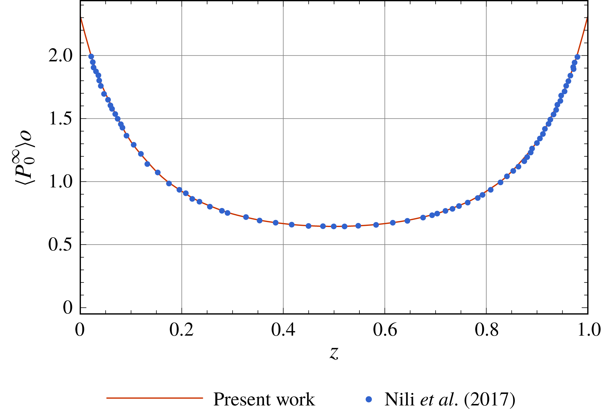
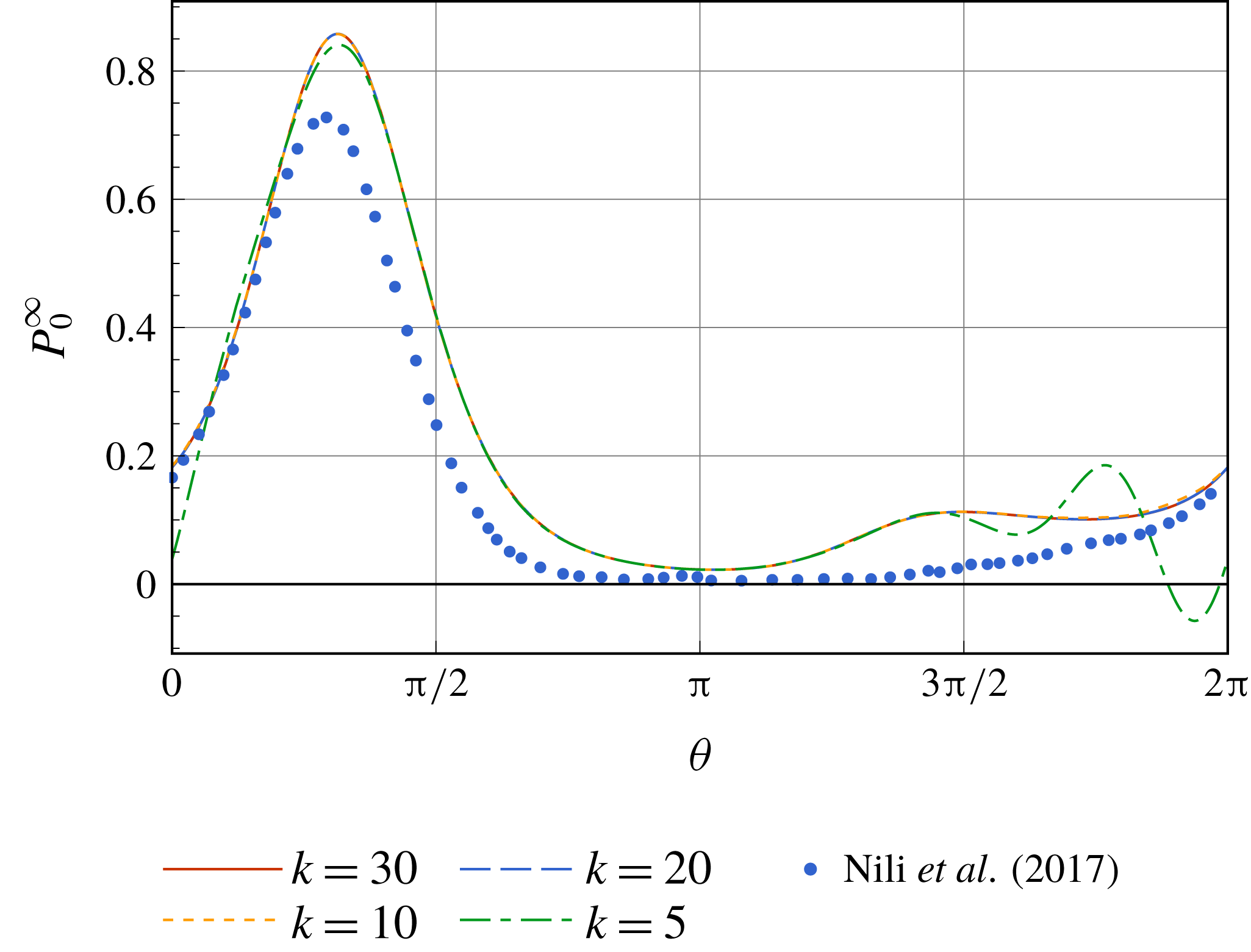
The orthogonality of the above function series gives rise to a system of linear equations of coefficients $A_{km}$ and $B_{km}$ . The truncation of the series gives a finite dimension of the constant coefficient matrix, and then the linear system is solved. This series expansion is verified with the numerical result of Nili et al. (Reference Nili, Kheyri, Abazari, Fahimniya and Naji2017), see appendix A.

In fact, the above approach to the solution of $G_{0}$ can also be applied to the evolution equation of $P_{0}(z,\unicode[STIX]{x1D703},t)$ , to obtain a system of ordinary differential equations (ODEs) of expansion coefficients with time variable $t$ ; $P_{0}$ exponentially decays to the asymptotic solution $P_{0}^{\infty }$ with time (Brenner & Edwards Reference Brenner and Edwards1993), i.e.

(4.17) $$\begin{eqnarray}P_{0}(z,\unicode[STIX]{x1D703},t)=P_{0}^{\infty }(z,\unicode[STIX]{x1D703})+\text{exp},\end{eqnarray}$$

where $\text{exp}$ denotes an exponential decay term with time.

4.2 First-order moment and overall advection velocity

Substituting (4.17) into (3.15) for $n=1$ gives

(4.18) $$\begin{eqnarray}{\displaystyle \frac{\text{d}M_{1}}{\text{d}t}}=\bar{U}+\text{exp},\end{eqnarray}$$

with

(4.19) $$\begin{eqnarray}\bar{U}\triangleq \int _{0}^{1}\int _{0}^{2\unicode[STIX]{x03C0}}[\mathit{Pe}_{f}U(z)+\mathit{Pe}_{s}\sin \unicode[STIX]{x1D703}]P_{0}^{\infty }(z,\unicode[STIX]{x1D703})\;\text{d}\unicode[STIX]{x1D703}\,\text{d}z,\end{eqnarray}$$

as the overall advection velocity. Then the first-order total moment is

(4.20) $$\begin{eqnarray}M_{1}=\bar{U}t+\bar{B}+\text{exp},\end{eqnarray}$$

where $\bar{B}$ is a constant to be determined.

Following Brenner & Edwards (Reference Brenner and Edwards1993), the asymptotic solution of $P_{1}$ is assumed to have the form

(4.21) $$\begin{eqnarray}P_{1}=P_{0}^{\infty }(z,\unicode[STIX]{x1D703})\bar{U}t+b(z,\unicode[STIX]{x1D703})+\text{exp},\end{eqnarray}$$

where $b(z,\unicode[STIX]{x1D703})$ is a trial function to be determined. In (3.2)–(38) in Brenner & Edwards (Reference Brenner and Edwards1993), $b(z,\unicode[STIX]{x1D703})=P_{0}^{\infty }(z,\unicode[STIX]{x1D703})B(z,\unicode[STIX]{x1D703})$ is used instead. Note that $b(z,\unicode[STIX]{x1D703})$ is the difference between the asymptotic global and local moments of the first order. The above assumption is based on the form (4.20) of $M_{1}$ . The equation for $b(z,\unicode[STIX]{x1D703})$ can be obtained by substituting $P_{1}$ (4.21) back into the first-order moment equation (3.8) ( $n=1$ ). Using (4.1) of $P_{0}^{\infty }$ , we have

(4.22) $$\begin{eqnarray}{\mathcal{L}}b(z,\unicode[STIX]{x1D703})=P_{0}^{\infty }(z,\unicode[STIX]{x1D703})[\mathit{Pe}_{f}U(z)+\mathit{Pe}_{s}\sin \unicode[STIX]{x1D703}-\bar{U}].\end{eqnarray}$$

The boundary conditions of $b(z,\unicode[STIX]{x1D703})$ are in the same form as those of $P_{0}^{\infty }$

(4.23) $$\begin{eqnarray}\displaystyle & \displaystyle {\displaystyle \frac{\unicode[STIX]{x2202}b}{\unicode[STIX]{x2202}z}}={\displaystyle \frac{1}{\unicode[STIX]{x1D6EC}\mathit{Pe}_{s}}}\cos \unicode[STIX]{x1D703}b,\quad \text{at }z=0,1, & \displaystyle\end{eqnarray}$$

(4.24) $$\begin{eqnarray}\displaystyle & \displaystyle b|_{\unicode[STIX]{x1D703}=0}=b|_{\unicode[STIX]{x1D703}=2\unicode[STIX]{x03C0}}, & \displaystyle\end{eqnarray}$$

(4.25) $$\begin{eqnarray}\displaystyle & \displaystyle \left.{\displaystyle \frac{\unicode[STIX]{x2202}b}{\unicode[STIX]{x2202}\unicode[STIX]{x1D703}}}\right|_{\unicode[STIX]{x1D703}=0}=\left.{\displaystyle \frac{\unicode[STIX]{x2202}b}{\unicode[STIX]{x2202}\unicode[STIX]{x1D703}}}\right|_{\unicode[STIX]{x1D703}=2\unicode[STIX]{x03C0}}. & \displaystyle\end{eqnarray}$$

Before solving $b(z,\unicode[STIX]{x1D703})$ , its relationship with constant $\bar{B}$ in (4.20) is shown. The cross-sectional integration of $P_{1}$ gives

(4.26) $$\begin{eqnarray}\bar{B}=\int _{0}^{1}\int _{0}^{2\unicode[STIX]{x03C0}}b(z,\unicode[STIX]{x1D703})\;\text{d}\unicode[STIX]{x1D703}\,\text{d}z.\end{eqnarray}$$

Note that constant $\bar{B}$ is not necessarily equal to zero, and it contains the information of the initial condition of $P$ , e.g. $m_{1\infty }$ in equation (39) in Aris (Reference Aris1956). Additionally, the solution of $b(z,\unicode[STIX]{x1D703})$ by (4.22) with boundary conditions (4.23), (4.24) and (4.25) is uniquely defined, although with an additive $cP_{0}^{\infty }(z,\unicode[STIX]{x1D703})$ , where $c$ is an arbitrary constant. Namely,

(4.27) $$\begin{eqnarray}b(z,\unicode[STIX]{x1D703})=b_{N}(z,\unicode[STIX]{x1D703})+\bar{B}P_{0}^{\infty }(z,\unicode[STIX]{x1D703}),\end{eqnarray}$$

where

(4.28) $$\begin{eqnarray}\int _{0}^{1}\int _{0}^{2\unicode[STIX]{x03C0}}b_{N}(z,\unicode[STIX]{x1D703})\;\text{d}\unicode[STIX]{x1D703}\,\text{d}z=0,\end{eqnarray}$$

is the normalization condition for $b_{N}(z,\unicode[STIX]{x1D703})$ in Hill & Bees (Reference Hill and Bees2002) and Manela & Frankel (Reference Manela and Frankel2003). Using $b_{N}(z,\unicode[STIX]{x1D703})$ instead of $b(z,\unicode[STIX]{x1D703})$ is enough to derive subsequent expressions of dispersion properties, see § 4.3. Thus we only consider the solution of the determinate $b_{N}(z,\unicode[STIX]{x1D703})$ .

The method of solving $b_{N}(z,\unicode[STIX]{x1D703})$ is similar to that for finding $P_{0}^{\infty }(z,\unicode[STIX]{x1D703})$ in (4.1), except with the inhomogeneous term on the right-hand side of (4.22). First, we decompose $b(z,\unicode[STIX]{x1D703})$ in the same form as (4.7) as

(4.29) $$\begin{eqnarray}b_{N}(z,\unicode[STIX]{x1D703})=P_{a}(z,\unicode[STIX]{x1D703})G_{b}(z,\unicode[STIX]{x1D703}),\end{eqnarray}$$

where $G_{b}(z,\unicode[STIX]{x1D703})$ satisfies

(4.30) $$\begin{eqnarray}{\mathcal{L}}_{0}G_{b}(z,\unicode[STIX]{x1D703})=G_{0}(z,\unicode[STIX]{x1D703})[\mathit{Pe}_{f}U(z)+\mathit{Pe}_{s}\sin \unicode[STIX]{x1D703}-\bar{U}].\end{eqnarray}$$

The boundary condition and periodic boundary conditions are the same as those for $G_{0}$ (4.12), (4.13) and (4.14), i.e.

(4.31) $$\begin{eqnarray}\displaystyle & \displaystyle {\displaystyle \frac{\unicode[STIX]{x2202}G_{b}}{\unicode[STIX]{x2202}z}}=0\quad \text{at }z=0,1., & \displaystyle\end{eqnarray}$$

(4.32) $$\begin{eqnarray}\displaystyle & \displaystyle G_{b}|_{\unicode[STIX]{x1D703}=0}=G_{b}|_{\unicode[STIX]{x1D703}=2\unicode[STIX]{x03C0}}, & \displaystyle\end{eqnarray}$$

(4.33) $$\begin{eqnarray}\displaystyle & \displaystyle \left.{\displaystyle \frac{\unicode[STIX]{x2202}G_{b}}{\unicode[STIX]{x2202}\unicode[STIX]{x1D703}}}\right|_{\unicode[STIX]{x1D703}=0}=\left.{\displaystyle \frac{\unicode[STIX]{x2202}G_{b}}{\unicode[STIX]{x2202}\unicode[STIX]{x1D703}}}\right|_{\unicode[STIX]{x1D703}=2\unicode[STIX]{x03C0}}. & \displaystyle\end{eqnarray}$$

Then one can perform a similar series expansion (4.16) for $G_{b}$ and solve the system of linear equations for corresponding coefficients.

4.3 Second-order moment and overall dispersivity

The second-order global moment is related to the overall dispersivity. Substituting (4.21) into (3.15) for $n=2$ gives

(4.34) $$\begin{eqnarray}{\displaystyle \frac{\text{d}M_{2}}{\text{d}t}}=2\bar{U}\bar{U}t+2\bar{B}\bar{U}+2(\bar{D}^{\text{M}}+\bar{D}^{\text{C}})+\text{exp},\end{eqnarray}$$

with

(4.35) $$\begin{eqnarray}\bar{D}^{\text{M}}\triangleq \int _{0}^{1}\int _{0}^{2\unicode[STIX]{x03C0}}\unicode[STIX]{x1D6EC}\mathit{Pe}_{s}^{2}P_{0}^{\infty }(z,\unicode[STIX]{x1D703})\;\text{d}\unicode[STIX]{x1D703}\,\text{d}z=\unicode[STIX]{x1D6EC}\mathit{Pe}_{s}^{2},\end{eqnarray}$$

as the ‘molecular’ dispersivity and

(4.36) $$\begin{eqnarray}\displaystyle \bar{D}^{\text{C}} & \triangleq & \displaystyle \int _{0}^{1}\int _{0}^{2\unicode[STIX]{x03C0}}b(z,\unicode[STIX]{x1D703})[\mathit{Pe}_{f}U(z)+\mathit{Pe}_{s}\sin \unicode[STIX]{x1D703}-\bar{U}]\;\text{d}\unicode[STIX]{x1D703}\,\text{d}z\nonumber\\ \displaystyle & = & \displaystyle \int _{0}^{1}\int _{0}^{2\unicode[STIX]{x03C0}}b_{N}(z,\unicode[STIX]{x1D703})[\mathit{Pe}_{f}U(z)+\mathit{Pe}_{s}\sin \unicode[STIX]{x1D703}]\;\text{d}\unicode[STIX]{x1D703}\,\text{d}z,\end{eqnarray}$$

as the ‘convective’ dispersivity (Brenner & Edwards Reference Brenner and Edwards1993). Therefore, the overall dispersivity is

(4.37) $$\begin{eqnarray}\bar{D}\triangleq {\displaystyle \frac{1}{2}}\lim _{t\rightarrow \infty }{\displaystyle \frac{\text{d}}{\text{d}t}}(M_{2}-M_{1}^{2})=\bar{D}^{\text{M}}+\bar{D}^{\text{C}}.\end{eqnarray}$$

Furthermore, the second-order local moment is also of interest. Subject to a posteriori verification, Shapiro & Brenner (Reference Shapiro and Brenner1987) constructed the asymptotic solution of $P_{2}$ with a time-independent function $\boldsymbol{H}(\boldsymbol{q})$ , namely, in our case

(4.38) $$\begin{eqnarray}P_{2}=P_{0}^{\infty }(z,\unicode[STIX]{x1D703})\left[\bar{U}\bar{U}t^{2}+2{\displaystyle \frac{b(z,\unicode[STIX]{x1D703})}{P_{0}^{\infty }(z,\unicode[STIX]{x1D703})}}\bar{U}t+2(\bar{D}^{\text{M}}+\bar{D}^{\text{C}})t+H(z,\unicode[STIX]{x1D703})\right]+\text{exp}.\end{eqnarray}$$

The boundary-value problem of $H(z,\unicode[STIX]{x1D703})$ can be found in equation (56) of Shapiro & Brenner (Reference Shapiro and Brenner1987).

Here we focus on the dispersivity for the local transport process. In a confined unidirectional flow, local dispersivity $D(z,\unicode[STIX]{x1D703})$ characterizes the dispersion process along each ‘streamline’ of the imposed flow in the local space. To define the local dispersivity, first we introduce the marginal probability density function along each local ‘streamline’ of the imposed flow by normalization of the local PDF

(4.39) $$\begin{eqnarray}P_{N}(x,z,\unicode[STIX]{x1D703},t)\triangleq {\displaystyle \frac{P(x,z,\unicode[STIX]{x1D703},t)}{P_{0}(z,\unicode[STIX]{x1D703},t)}},\end{eqnarray}$$

for each point $(z,\unicode[STIX]{x1D703})$ in the cross-section $Oz\unicode[STIX]{x1D703}$ . Thus the moment of $P_{N}$ is

(4.40) $$\begin{eqnarray}P_{Nn}(z,\unicode[STIX]{x1D703},t)\triangleq \int _{-\infty }^{\infty }x^{n}P_{N}(x,z,\unicode[STIX]{x1D703},t)\;\text{d}x={\displaystyle \frac{P_{n}(z,\unicode[STIX]{x1D703},t)}{P_{0}(z,\unicode[STIX]{x1D703},t)}},\quad n=0,1,\ldots .\end{eqnarray}$$

Then local dispersivity $D(z,\unicode[STIX]{x1D703})$ is defined as

(4.41) $$\begin{eqnarray}D(z,\unicode[STIX]{x1D703})\triangleq {\displaystyle \frac{1}{2}}\lim _{t\rightarrow \infty }{\displaystyle \frac{\text{d}}{\text{d}t}}(P_{N2}-P_{N1}^{2}),\end{eqnarray}$$

as the ‘Taylor dispersivity’ of the distribution along each local ‘streamline’ of the imposed flow.

The long-time asymptotic values of $P_{Nn}$ are

(4.42) $$\begin{eqnarray}\lim _{t\rightarrow \infty }P_{Nn}={\displaystyle \frac{1}{P_{0}^{\infty }(z,\unicode[STIX]{x1D703})}}\lim _{t\rightarrow \infty }P_{n},\quad n=1,2,\ldots .\end{eqnarray}$$

Introduction of $P_{2}$ (4.38) and $P_{1}$ (4.21) into (4.41) gives

(4.43) $$\begin{eqnarray}D=\bar{D}^{\text{M}}+\bar{D}^{\text{C}}=\bar{D}.\end{eqnarray}$$

The local dispersivity is the same as the Taylor dispersivity. Namely, after a long time, there is no cross-sectional ( $Oz\unicode[STIX]{x1D703}$ ) difference in dispersivity among streamlines of the imposed flow (Wu & Chen Reference Wu and Chen2014), resulting from the leading-order term of time in the GTD theory.

4.4 Long-time asymptotic expansion of $\langle P\rangle$ and $P$

Now we can perform the second-order cumulant expansion of global PDF $\langle P\rangle$ and local PDF $P(x,z,\unicode[STIX]{x1D703},t)$ (Chatwin Reference Chatwin1970; Frankel & Brenner Reference Frankel and Brenner1989; Guo et al. Reference Guo, Wu, Jiang and Chen2018; Jiang & Chen Reference Jiang and Chen2018, Reference Jiang and Chen2019). We have obtained the required coefficients, i.e. overall advection velocity $\bar{U}$ (4.19) and overall dispersivity $\bar{D}$ (4.37), as well as local dispersivity $D$ (4.43).

The second-order cumulant expansion is a Gaussian distribution, namely,

(4.44) $$\begin{eqnarray}\displaystyle & \displaystyle \langle P\rangle (x,t)\approx {\displaystyle \frac{1}{2\sqrt{\unicode[STIX]{x03C0}\bar{D}t}}}\exp \left[{\displaystyle \frac{(x-\bar{U}t)^{2}}{4\bar{D}t}}\right], & \displaystyle\end{eqnarray}$$

(4.45) $$\begin{eqnarray}\displaystyle & \displaystyle P(x,z,\unicode[STIX]{x1D703},t)\approx P_{0}^{\infty }(z,\unicode[STIX]{x1D703})\langle P\rangle (x,t). & \displaystyle\end{eqnarray}$$

Note that the cumulant expansion for $P$ is performed along each ‘streamline’ of the imposed flow in the cross-section $Oz\unicode[STIX]{x1D703}$ . Higher-order terms are omitted here, which requires the coefficients like skewness and kurtosis (Frankel & Brenner Reference Frankel and Brenner1989; Wang & Chen Reference Wang and Chen2017).

5.1 Extended flow field

Figure 2.

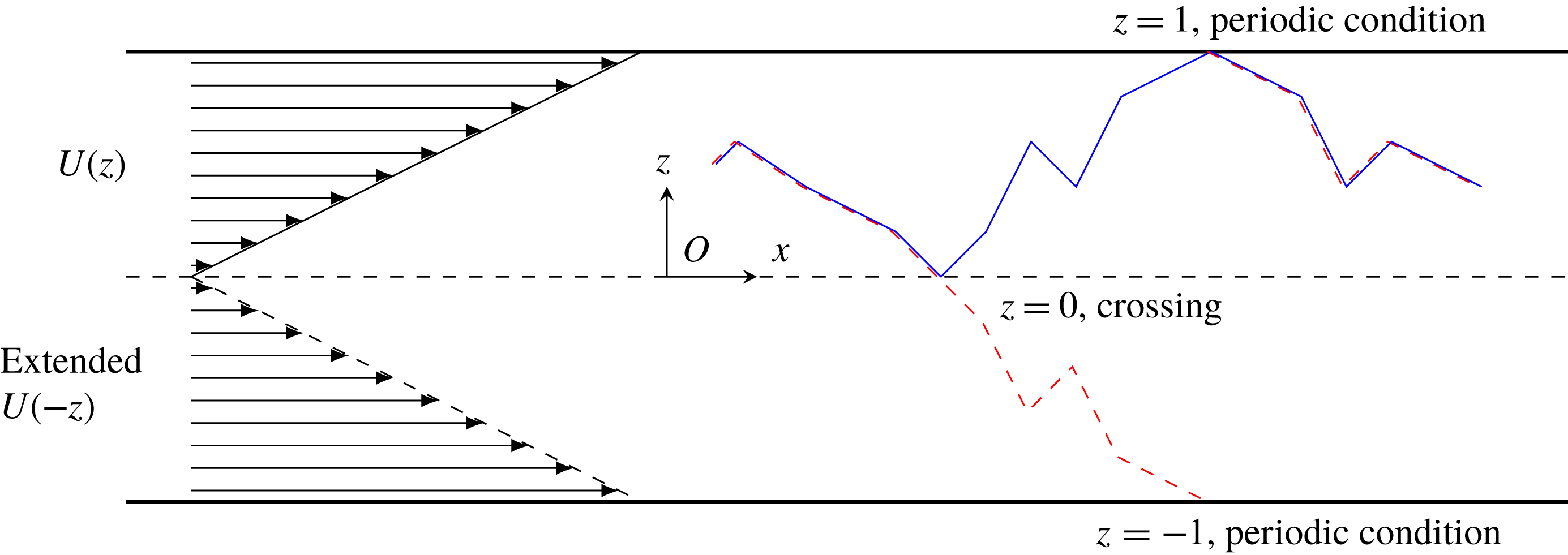
Paths of an active particle in the extended flow field. The actual path is shown with a blue solid line, and the extended path with a red dashed line. The particle hitting the boundary $z=0$ is considered as crossing the boundary with the same swimming direction. The boundaries $z=1$ and $z=-1$ are periodic. Namely, the particle hitting the boundary $z=1$ is then seen as swimming on the other side of the boundary ( $z=-1$ ), and vice versa.

The original transport problem of active particles with the reflection boundary condition is reconstructed as a transport problem with periodic boundary conditions at $z=\pm 1$ , in the extended flow field as shown in figure 2, with extended velocity

(5.1) $$\begin{eqnarray}U_{E}(z)=\left\{\begin{array}{@{}ll@{}}U(z), & 0\leqslant z\leqslant 1,\\ U(-z), & -1\leqslant z<0,\end{array}\right.\end{eqnarray}$$

defined by a piecewise function. The corresponding extended angular velocity $\unicode[STIX]{x1D6FA}_{E}(z,\unicode[STIX]{x1D703})$ is

(5.2) $$\begin{eqnarray}\unicode[STIX]{x1D6FA}_{E}(z,\unicode[STIX]{x1D703})=\left\{\begin{array}{@{}ll@{}}\unicode[STIX]{x1D6FA}(z,\unicode[STIX]{x1D703}), & 0\leqslant z\leqslant 1,\\ -\unicode[STIX]{x1D6FA}(-z,\unicode[STIX]{x03C0}-\unicode[STIX]{x1D703}), & -1\leqslant z<0.\end{array}\right.\end{eqnarray}$$

Note that the angular velocity may be discontinuous at boundaries $z=\pm 1$ and $z=0$ .

The whole problem (2.18) and (2.21)–(2.24) becomes

(5.3) $$\begin{eqnarray}\displaystyle & \displaystyle {\displaystyle \frac{\unicode[STIX]{x2202}P_{E}}{\unicode[STIX]{x2202}t}}+[\mathit{Pe}_{f}\unicode[STIX]{x1D6FA}_{E}(z)+\mathit{Pe}_{s}\sin \unicode[STIX]{x1D703}]{\displaystyle \frac{\unicode[STIX]{x2202}P_{E}}{\unicode[STIX]{x2202}x}}-\unicode[STIX]{x1D6EC}\mathit{Pe}_{s}^{2}{\displaystyle \frac{\unicode[STIX]{x2202}^{2}P_{E}}{\unicode[STIX]{x2202}x^{2}}}+{\mathcal{L}}_{E}P_{E}=0,\quad -1\leqslant z<1, & \displaystyle\end{eqnarray}$$

(5.4) $$\begin{eqnarray}\displaystyle & \displaystyle P_{E}|_{\unicode[STIX]{x1D703}=0}=P_{E}|_{\unicode[STIX]{x1D703}=2\unicode[STIX]{x03C0}}, & \displaystyle\end{eqnarray}$$

(5.5) $$\begin{eqnarray}\displaystyle & \displaystyle \left.{\displaystyle \frac{\unicode[STIX]{x2202}P_{E}}{\unicode[STIX]{x2202}\unicode[STIX]{x1D703}}}\right|_{\unicode[STIX]{x1D703}=0}=\left.{\displaystyle \frac{\unicode[STIX]{x2202}P_{E}}{\unicode[STIX]{x2202}\unicode[STIX]{x1D703}}}\right|_{\unicode[STIX]{x1D703}=2\unicode[STIX]{x03C0}}, & \displaystyle\end{eqnarray}$$

(5.6) $$\begin{eqnarray}\displaystyle & \displaystyle P_{E}|_{z=-1}=P_{E}|_{z=1}, & \displaystyle\end{eqnarray}$$

(5.7) $$\begin{eqnarray}\displaystyle & \displaystyle \left.{\displaystyle \frac{\unicode[STIX]{x2202}P_{E}}{\unicode[STIX]{x2202}z}}\right|_{z=-1}=\left.{\displaystyle \frac{\unicode[STIX]{x2202}P_{E}}{\unicode[STIX]{x2202}z}}\right|_{z=1}, & \displaystyle\end{eqnarray}$$

(5.8) $$\begin{eqnarray}\displaystyle & \displaystyle P_{E}|_{t=0}=P_{E}^{(0)}(x,z,\unicode[STIX]{x1D703})=\left\{\begin{array}{@{}ll@{}}{\textstyle \frac{1}{2}}P^{(0)}(x,z,\unicode[STIX]{x1D703}), & 0\leqslant z\leqslant 1,\\ {\textstyle \frac{1}{2}}P^{(0)}(x,-z,\unicode[STIX]{x03C0}-\unicode[STIX]{x1D703}), & -1\leqslant z<0,\end{array}\right. & \displaystyle\end{eqnarray}$$

where $P_{E}$ is the extended PDF. The operator ${\mathcal{L}}_{E}$ is analogous to ${\mathcal{L}}$ (2.19) as

(5.9) $$\begin{eqnarray}{\mathcal{L}}_{E}(\boldsymbol{\cdot })=\mathit{Pe}_{s}\cos \unicode[STIX]{x1D703}{\displaystyle \frac{\unicode[STIX]{x2202}}{\unicode[STIX]{x2202}z}}(\boldsymbol{\cdot })+{\displaystyle \frac{\unicode[STIX]{x2202}}{\unicode[STIX]{x2202}\unicode[STIX]{x1D703}}}\left[\unicode[STIX]{x1D6FA}_{E}(z,\unicode[STIX]{x1D703})(\boldsymbol{\cdot })-{\displaystyle \frac{\unicode[STIX]{x2202}}{\unicode[STIX]{x2202}\unicode[STIX]{x1D703}}}(\boldsymbol{\cdot })\right]-\unicode[STIX]{x1D6EC}\mathit{Pe}_{s}^{2}{\displaystyle \frac{\unicode[STIX]{x2202}^{2}}{\unicode[STIX]{x2202}z^{2}}}(\boldsymbol{\cdot }),\end{eqnarray}$$

in replacing $\unicode[STIX]{x1D6FA}(z,\unicode[STIX]{x1D703})$ with $\unicode[STIX]{x1D6FA}_{E}(z,\unicode[STIX]{x1D703})$ ; $P_{E}^{(0)}(x,z,\unicode[STIX]{x1D703})$ is the extended initial condition. Note that the reflection boundary condition (2.14) of $P$ has been replaced with periodic boundary conditions (5.6) and (5.7) of $P_{E}$ .

To obtain the original PDF $P(x,z,\unicode[STIX]{x1D703},t)$ , one needs to make a linear superposition of $P_{E}$ of the two regions $-1\leqslant z<0$ and $0\leqslant z\leqslant 1$ with a transformation as

(5.10) $$\begin{eqnarray}P(x,z,\unicode[STIX]{x1D703},t)=P_{E}(x,z,\unicode[STIX]{x1D703},t)+P_{E}(x,-z,\unicode[STIX]{x03C0}-\unicode[STIX]{x1D703},t),\quad 0\leqslant z\leqslant 1.\end{eqnarray}$$

The continuity of PDF $P_{E}$ at $z=0$ and the periodic boundary conditions (5.6) and (5.7) at $z=\pm 1$ ensure that $P$ obtained by (5.10) satisfies the reflection boundary condition (2.14) as

(5.11) $$\begin{eqnarray}\displaystyle P(x,1,\unicode[STIX]{x1D703},t) & = & \displaystyle P_{E}(x,1,\unicode[STIX]{x1D703},t)+P_{E}(x,-1,\unicode[STIX]{x03C0}-\unicode[STIX]{x1D703},t),\nonumber\\ \displaystyle & = & \displaystyle P_{E}(x,-1,\unicode[STIX]{x1D703},t)+P_{E}(x,1,\unicode[STIX]{x03C0}-\unicode[STIX]{x1D703},t),\nonumber\\ \displaystyle & = & \displaystyle P_{E}(x,1,\unicode[STIX]{x03C0}-\unicode[STIX]{x1D703},t)+P_{E}(x,-1,\unicode[STIX]{x1D703},t),\nonumber\\ \displaystyle & = & \displaystyle P(x,1,\unicode[STIX]{x03C0}-\unicode[STIX]{x1D703},t),\end{eqnarray}$$

and

(5.12) $$\begin{eqnarray}\displaystyle P(x,0,\unicode[STIX]{x1D703},t) & = & \displaystyle P_{E}(x,0,\unicode[STIX]{x1D703},t)+P_{E}(x,0,\unicode[STIX]{x03C0}-\unicode[STIX]{x1D703},t),\nonumber\\ \displaystyle & = & \displaystyle P_{E}(x,0,\unicode[STIX]{x03C0}-\unicode[STIX]{x1D703},t)+P_{E}(x,0,\unicode[STIX]{x1D703},t),\nonumber\\ \displaystyle & = & \displaystyle P(x,0,\unicode[STIX]{x03C0}-\unicode[STIX]{x1D703},t).\end{eqnarray}$$

Note that there is a symmetric structure of the extended transport problem as constructed above. The operator ${\mathcal{L}}_{E}$ is symmetric with respect to the reflection transformation

(5.13a,b ) $$\begin{eqnarray}z\rightarrow -z,\quad \unicode[STIX]{x1D703}\rightarrow \unicode[STIX]{x03C0}-\unicode[STIX]{x1D703}.\end{eqnarray}$$

Note that the extended initial condition $P_{E}^{(0)}(x,z,\unicode[STIX]{x1D703})$ (5.8) is also constructed to satisfy the above reflection transformation (5.13). Therefore, one has

(5.14) $$\begin{eqnarray}P_{E}(x,z,\unicode[STIX]{x1D703},t)=P_{E}(x,-z,\unicode[STIX]{x03C0}-\unicode[STIX]{x1D703},t),\end{eqnarray}$$

and can replace the transformation (5.10) with a simple one as

(5.15) $$\begin{eqnarray}P(x,z,\unicode[STIX]{x1D703},t)=2P_{E}(x,z,\unicode[STIX]{x1D703},t),\quad 0\leqslant z\leqslant 1,\end{eqnarray}$$

for the original PDF.

5.2 Solution of long-time asymptotic moments

Now the generalized Taylor dispersion theory (§§ 3.2 and 4) can be applied to the extended problem without difficulties, by changing the integration region of $z$ and employment of the extended flow field $U_{E}(z)$ (5.1) and the extended local operator ${\mathcal{L}}_{E}$ (5.9). The corresponding global and local moments (3.5) and (3.6), overall advection velocity $\bar{U}$ (4.19) and dispersivity $\bar{D}$ (4.37) are redefined and are denoted by subscript $E$ , with $\langle \rangle _{E}$ to denote the integration over the extended cross-section as

(5.16) $$\begin{eqnarray}\langle P_{E}\rangle _{E}\triangleq \int _{-1}^{1}\int _{0}^{2\unicode[STIX]{x03C0}}P_{E}(x,z,\unicode[STIX]{x1D703},t)\;\text{d}\unicode[STIX]{x1D703}\,\text{d}z.\end{eqnarray}$$

Detailed solutions are illustrated in appendix B.

6.1 Local distribution $P_{0}^{\infty }(z,\unicode[STIX]{x1D703})$

The long-time asymptotic zeroth-order moment $P_{0}^{\infty }(z,\unicode[STIX]{x1D703})$ is the marginal probability density in the cross-section $Oz\unicode[STIX]{x1D703}$ , which characterizes the local distribution (Ezhilan & Saintillan Reference Ezhilan and Saintillan2015; Nili et al. Reference Nili, Kheyri, Abazari, Fahimniya and Naji2017). To compare the influence of velocity profiles on dispersion processes, we use various flow Péclet numbers $\mathit{Pe}_{f}$ , with a constant swimming Péclet number $\mathit{Pe}_{s}=1$ and $\unicode[STIX]{x1D6EC}=1/6$ in all cases.

6.1.1 The reflection boundary condition

In the absence of flow, as shown by Ezhilan & Saintillan (Reference Ezhilan and Saintillan2015), the solution of local distribution $P_{0}^{\infty }(z,\unicode[STIX]{x1D703})$ is a constant, without wall accumulation. This special solution can be generalized for spherical particles in the imposed flows.

Note that both the angular velocities are independent of $\unicode[STIX]{x1D703}$ . Thus  (B 1) for the asymptotic state of the zeroth-order moment of the extended PDF $P_{E0}^{\infty }$ is simplified as

(6.7) $$\begin{eqnarray}\mathit{Pe}_{s}\cos \unicode[STIX]{x1D703}{\displaystyle \frac{\unicode[STIX]{x2202}P_{E0}^{\infty }}{\unicode[STIX]{x2202}z}}+\unicode[STIX]{x1D6FA}_{E}(z){\displaystyle \frac{\unicode[STIX]{x2202}P_{E0}^{\infty }}{\unicode[STIX]{x2202}\unicode[STIX]{x1D703}}}-{\displaystyle \frac{\unicode[STIX]{x2202}^{2}P_{E0}^{\infty }}{\unicode[STIX]{x2202}\unicode[STIX]{x1D703}^{2}}}-\unicode[STIX]{x1D6EC}\mathit{Pe}_{s}^{2}{\displaystyle \frac{\unicode[STIX]{x2202}^{2}P_{E0}^{\infty }}{\unicode[STIX]{x2202}z^{2}}}=0.\end{eqnarray}$$

Therefore, with the periodic boundary conditions (B 3), (B 4), (B 5) and (B 6), the above partial differential equation has a constant solution

(6.8) $$\begin{eqnarray}P_{E0}^{\infty }=\frac{1}{4\unicode[STIX]{x03C0}}.\end{eqnarray}$$

Thus the solution for the original transport problem (4.1) with reflection boundary conditions (3.12) is

(6.9) $$\begin{eqnarray}P_{0}^{\infty }=\frac{1}{2\unicode[STIX]{x03C0}}.\end{eqnarray}$$

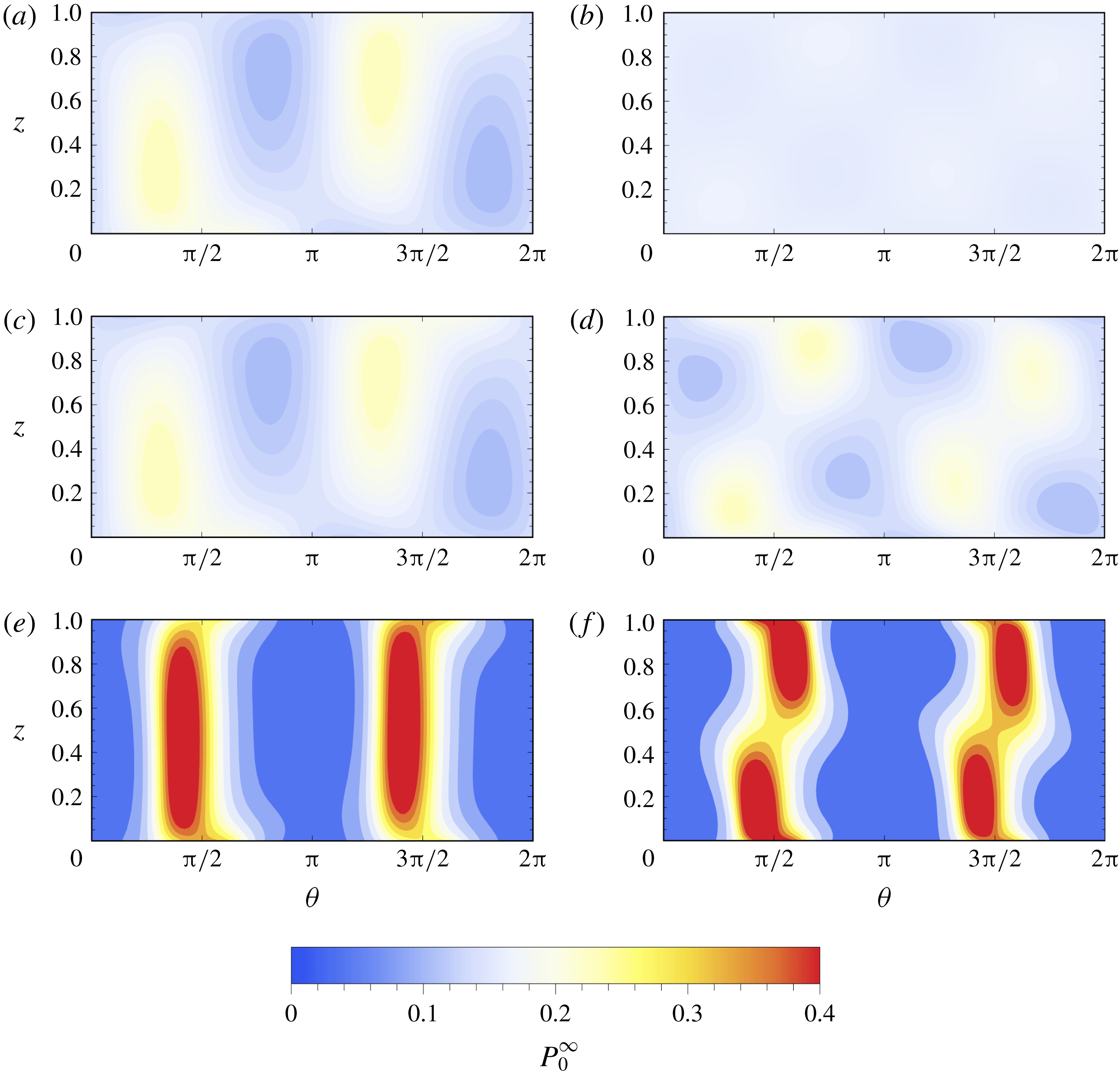
6.1.2 The Robin boundary condition and wall accumulation

Figure 3.

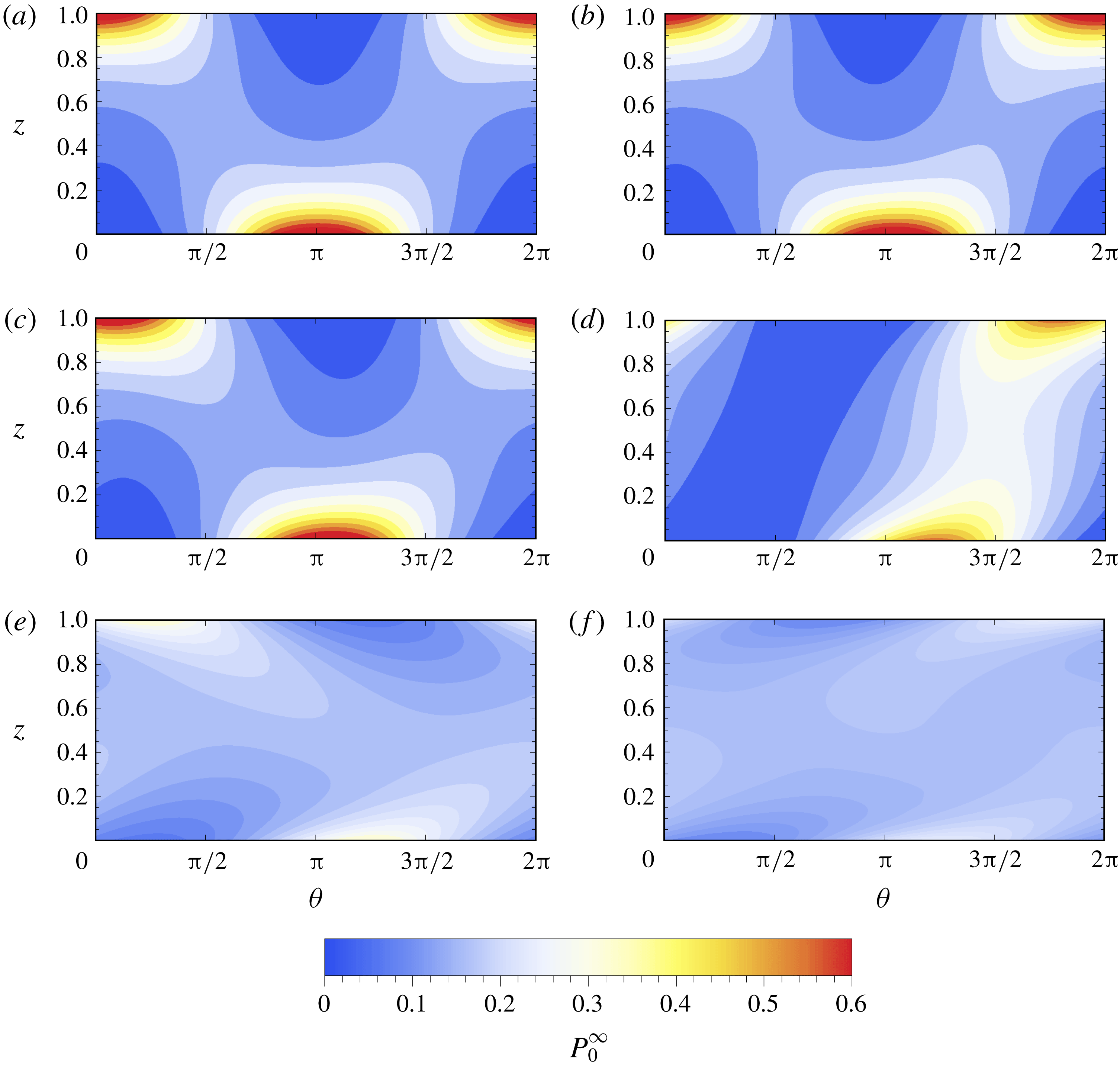
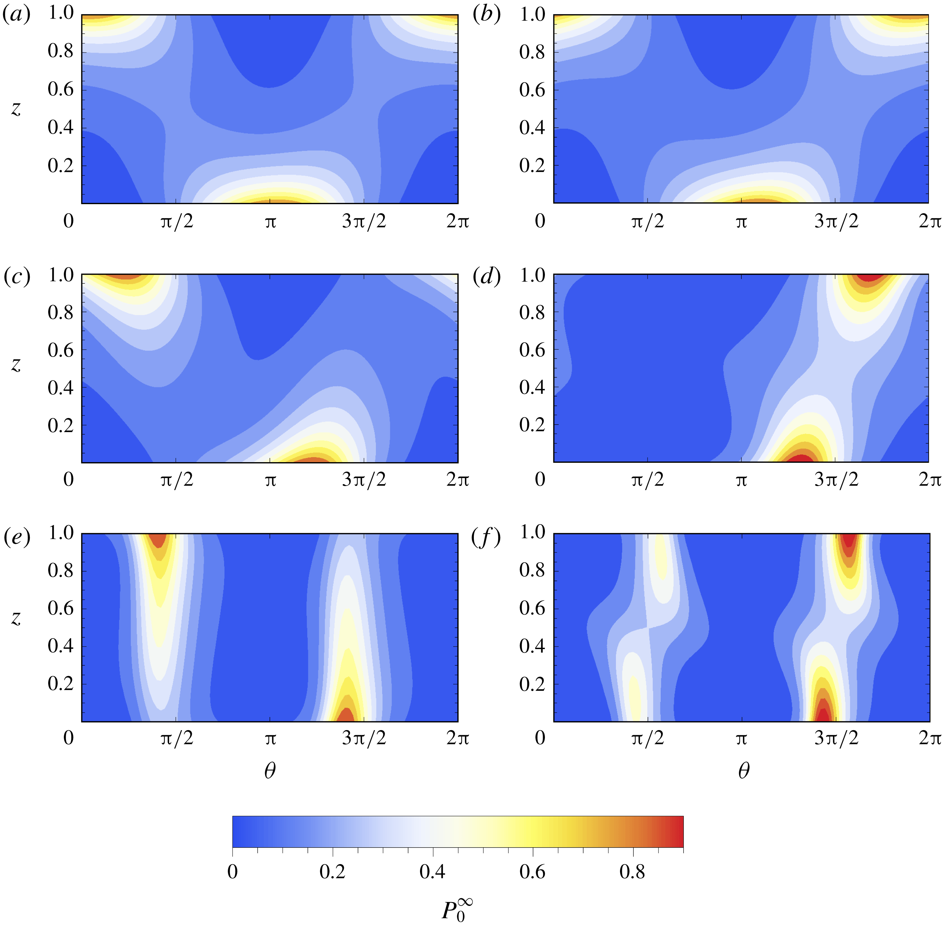
Density plot of local distributions $P_{0}^{\infty }(z,\unicode[STIX]{x1D703})$ (4.7) and (4.16) of spherical active particles in the two studied flows with various flow Péclet numbers $\mathit{Pe}_{f}$ , under the Robin condition (2.20). (a,c,e) Couette flow; (b,d,f) plane Poiseuille flow. (a,b)  $\mathit{Pe}_{f}=0.1$ ; (c,d)  $\mathit{Pe}_{f}=1$ ; (e,f)  $\mathit{Pe}_{f}=10$ . In all cases, $\unicode[STIX]{x1D6FC}_{0}=0$ , $\mathit{Pe}_{s}=1$ , $\unicode[STIX]{x1D6EC}=1/6$ .

For the reflection boundary condition, the local distribution $P_{0}^{\infty }$ for dispersion of spherical active particles in confined flows is uniform, without wall accumulation. In contrast, the complicated results with the Robin boundary condition of the local distribution are shown in figure 3 to illustrate how the velocity profile shapes the wall-normal polarization structure of $P_{0}^{\infty }(z,\unicode[STIX]{x1D703})$ . Obviously, the symmetric structures (6.5) and (6.6) of velocity profiles lead to the corresponding symmetric streamwise changes in the polarization. With high flow Péclet numbers $\mathit{Pe}_{f}$ , the polarization is suppressed by the shear alignments.

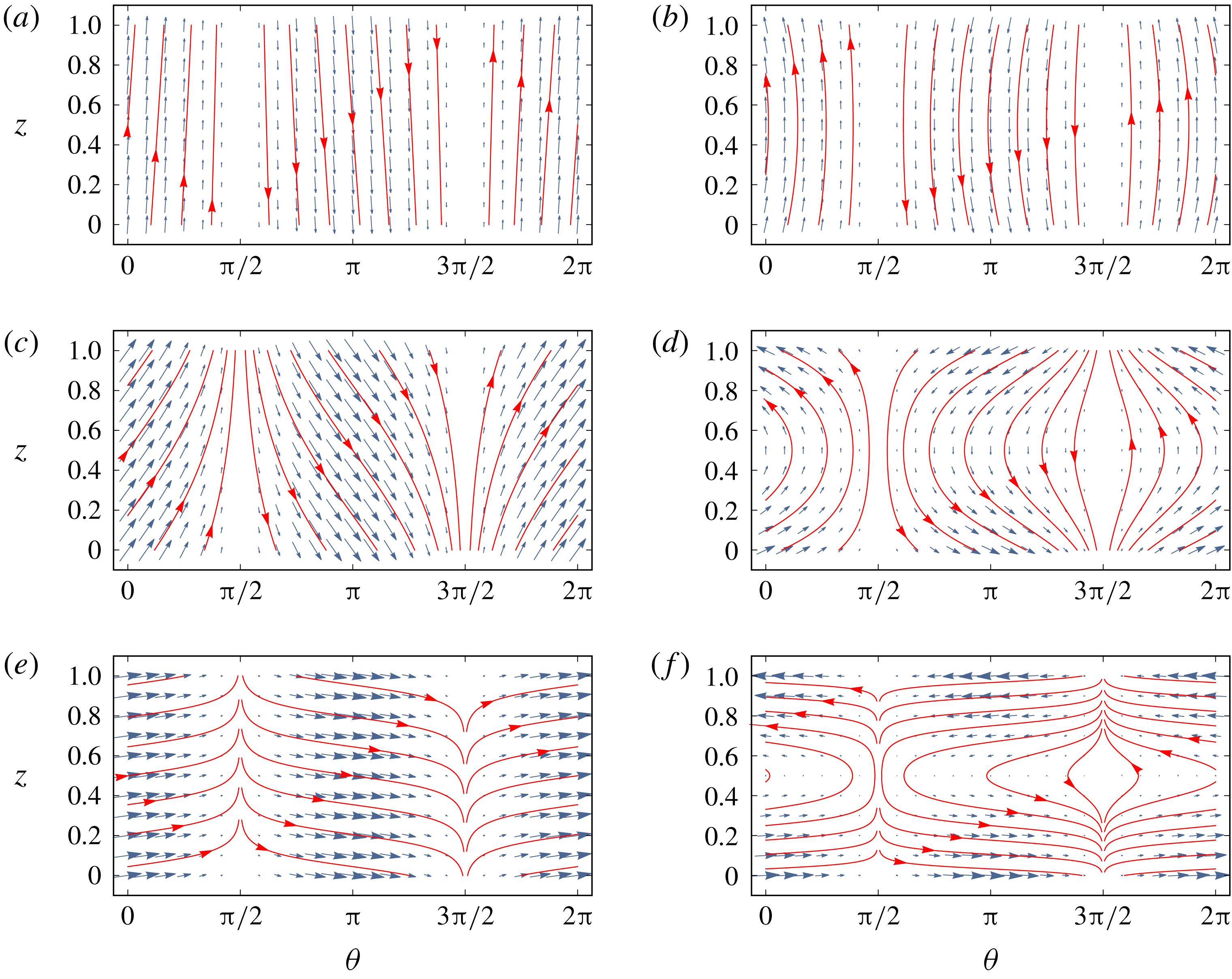
Here we discuss the structure of the local distribution $P_{0}^{\infty }(z,\unicode[STIX]{x1D703})$ in a more intuitive way; $P_{0}^{\infty }(z,\unicode[STIX]{x1D703})$ is exactly the solution for a local distribution in the cross-section $Oz\unicode[STIX]{x1D703}$ . Based on the GTD theory, we can define a local velocity vector in the local space $Oz\unicode[STIX]{x1D703}$ as

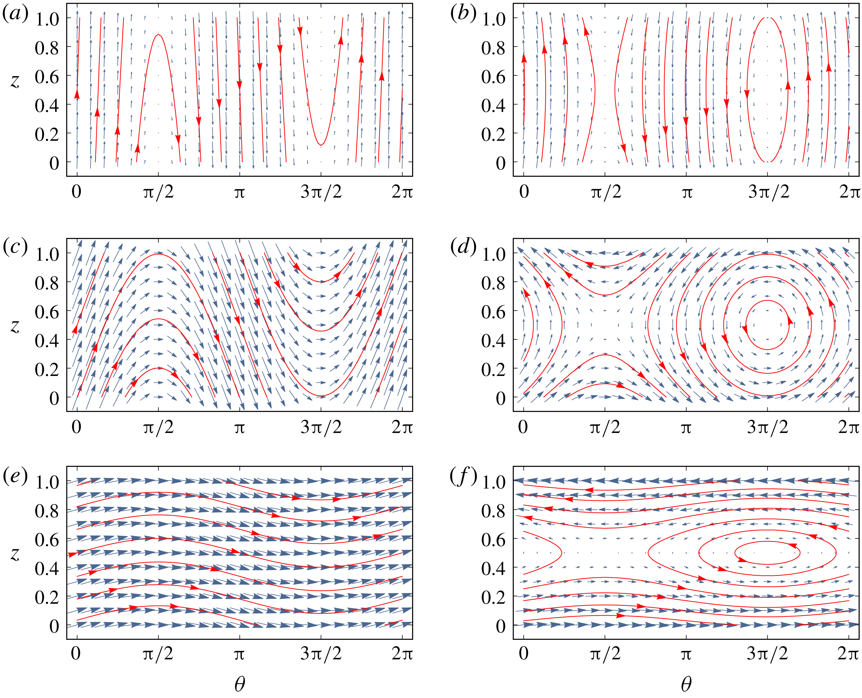
(6.10) $$\begin{eqnarray}\boldsymbol{u}=(\mathit{Pe}_{s}\cos \unicode[STIX]{x1D703},\unicode[STIX]{x1D6FA}(z,\unicode[STIX]{x1D703})),\end{eqnarray}$$

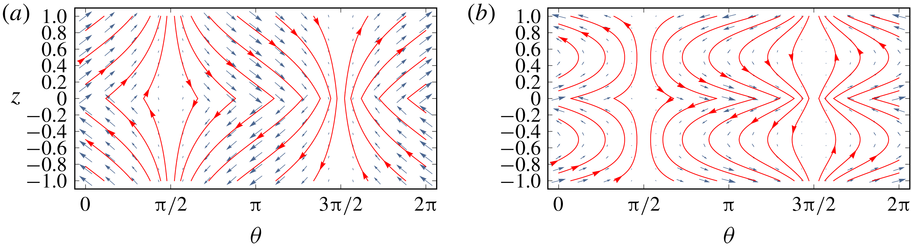
as shown in figure 4 for the studied cases. If the diffusion terms in (4.1) are neglected, the transport problem becomes a dynamical system (Zöttl & Stark Reference Zöttl and Stark2012, Reference Zöttl and Stark2013). Swimmers accumulate near stable critical points and lines (with zero local velocity). They also accumulate near the walls with the Robin boundary condition (2.13), as balanced by the diffusion effect.

Figure 4.

Local velocity vector $\boldsymbol{u}$ (6.10) fields for spherical particles in the local space $\boldsymbol{q}=(z,\unicode[STIX]{x1D703})$ , with various flow Péclet numbers $\mathit{Pe}_{f}$ , under the Robin condition (2.20). (a,c,e) Couette flow; (b,d,f) plane Poiseuille flow. (a,b)  $\mathit{Pe}_{f}=0.1$ ; (c,d)  $\mathit{Pe}_{f}=1$ ; (e,f)  $\mathit{Pe}_{f}=10$ . Red lines are streamlines.

In the case with low flow Péclet numbers $\mathit{Pe}_{f}$ , shown in figures 3(a,b) and 4(a,b), the swimming effect is dominant. Active particles swim through the ‘streamlines’ and finally accumulate near the point $(0,\unicode[STIX]{x03C0})$ at the back wall and $(1,2\unicode[STIX]{x03C0})$ at the front wall of the channel (Elgeti & Gompper Reference Elgeti and Gompper2013) in both flows. Namely, they swim towards the walls. With a larger $\mathit{Pe}_{f}$ , the global velocity field $U(z)$ leads to a larger angular velocity $\unicode[STIX]{x1D6FA}(z)$ , independent of $\unicode[STIX]{x1D703}$ . The accumulation is weakened by the strong shear rate of the flow. Because the wall-normal polarization due to the swimming behaviour is suppressed by the rapid rotation of particles, few streamlines end at the walls.

Furthermore, the local velocity fields $\boldsymbol{u}$ of the two flows are fundamentally different. The vorticity of Couette flow is uniform. To balance the rotation flux of particles, the accumulating points of swimmers move towards points $(0,3\unicode[STIX]{x03C0}/2)$ (upstream) and $(1,\unicode[STIX]{x03C0}/2)$ (downstream) when the flow Péclet number $\mathit{Pe}_{f}$ is large, shown in figures 3(c,e) and 4(c,e). However, for the plane Poiseuille flow shown in figures 3(d,f) and 4(d,f), the accumulating regions are near $(0,3\unicode[STIX]{x03C0}/2)$ and $(1,3\unicode[STIX]{x03C0}/2)$ (both upstream), due to the different shear alignments towards the wall. In addition, $\boldsymbol{u}$ has closed orbits in the middle of the channel (Zöttl & Stark Reference Zöttl and Stark2012), as shown in figure 4(b,d,f). The spherical particles stay and swing in weak shear-rate regions (in the centre of the channel), where the swimming effect is balanced by the rotation by the imposed flow. This swinging effect can weaken the accumulation near the channel walls, where particles have periodic tumbling motion.

Figure 5.

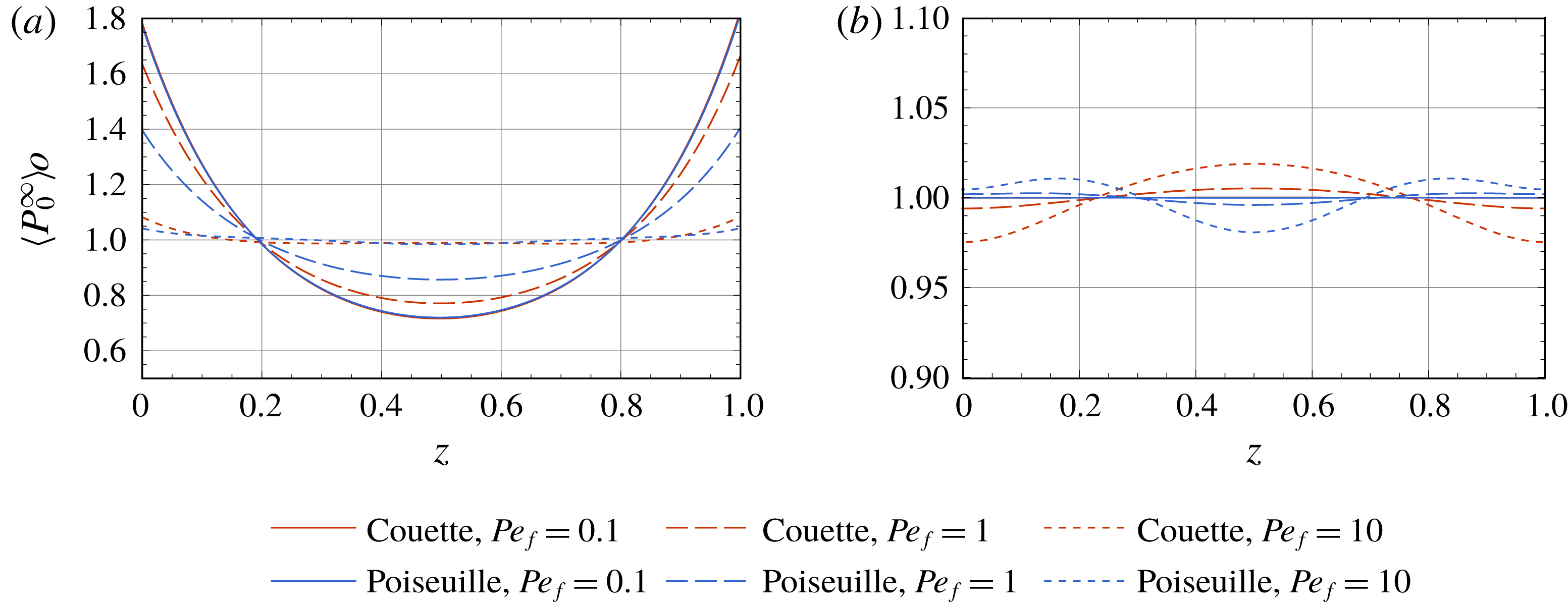
Orientation-space mean PDF $\langle P_{0}^{\infty }\rangle _{O}$ (6.11) of spherical active particles with various flow Péclet numbers $\mathit{Pe}_{f}$ , under the Robin condition (2.20). ‘Couette’ denotes the Couette flow, and ‘Poiseuille’ denotes the plane Poiseuille flow. In all cases, $\unicode[STIX]{x1D6FC}_{0}=0$ , $\mathit{Pe}_{s}=1$ , $\unicode[STIX]{x1D6EC}=1/6$ .

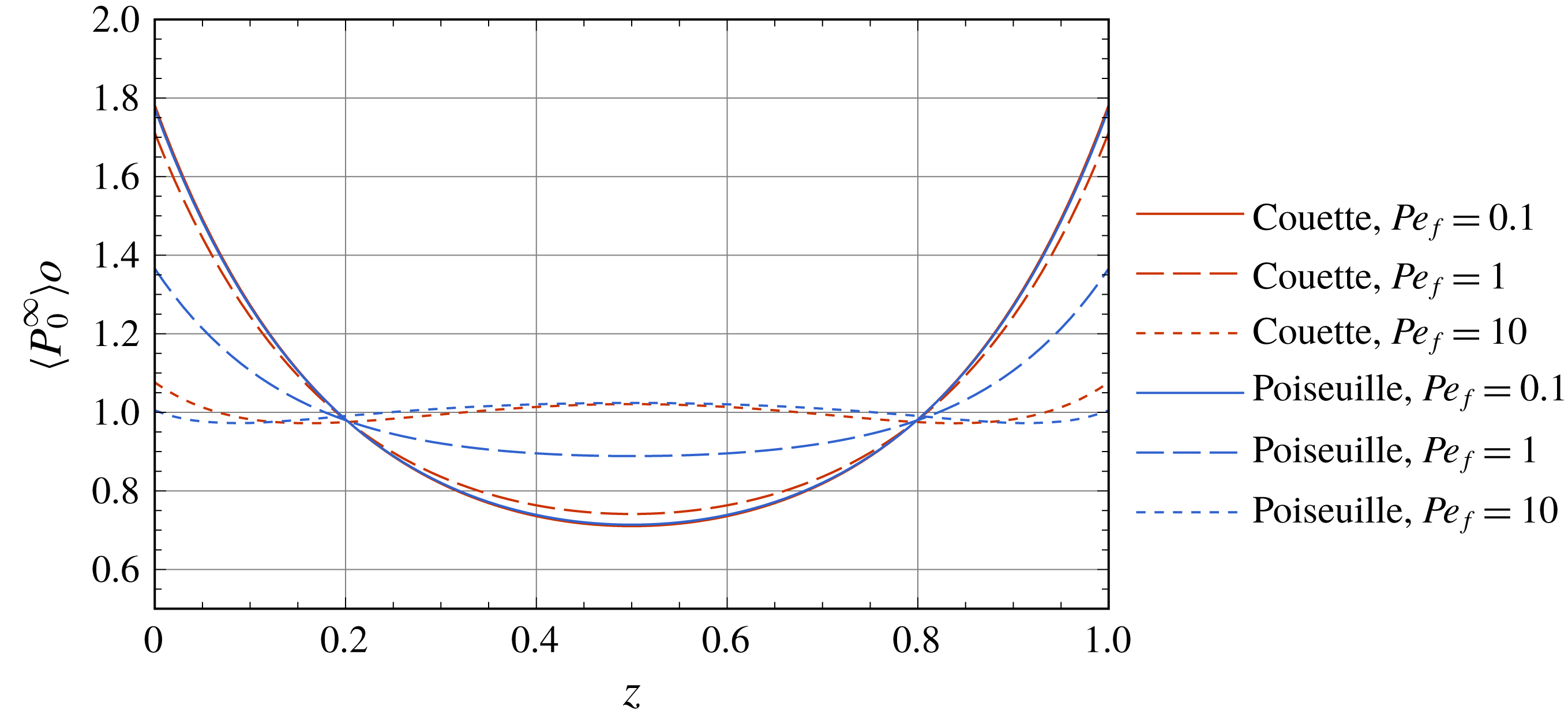
The accumulation of swimmers at the channel walls can be illustrated more clearly in terms of the orientation-space mean PDF

(6.11) $$\begin{eqnarray}\langle P_{0}^{\infty }\rangle _{O}\triangleq \int _{0}^{2\unicode[STIX]{x03C0}}P_{0}^{\infty }(z,\unicode[STIX]{x1D703})\;\text{d}\unicode[STIX]{x1D703},\end{eqnarray}$$

i.e. the marginal probability density in the transverse direction, as shown in figure 5. A large shear rate of global velocity (large $\mathit{Pe}_{f}$ ) can reduce the wall accumulation by the rapid rotation of particles. The reduction is stronger for the plane Poiseuille flow than in the Couette flow, because the varied shear rate of the plane Poiseuille flow across the channel is much larger near the boundaries.

6.2 Overall advection velocity $\bar{U}$ and dispersivity $\bar{D}$

In the confined cross-section $Oz\unicode[STIX]{x1D703}$ , the asymptotic zeroth-order moment $P_{0}^{\infty }(z,\unicode[STIX]{x1D703})$ provides a basic local distribution. The Robin boundary condition leads to the wall accumulation, while the local distribution under the reflection boundary condition is uniform. In the longitudinal direction, the advection velocity $\bar{U}$ and dispersivity $\bar{D}$ can characterize the overall dispersion process of active particles. Here the influence of boundary conditions on these dispersion properties is presented. The velocity profiles on the local distribution will also shape these properties.

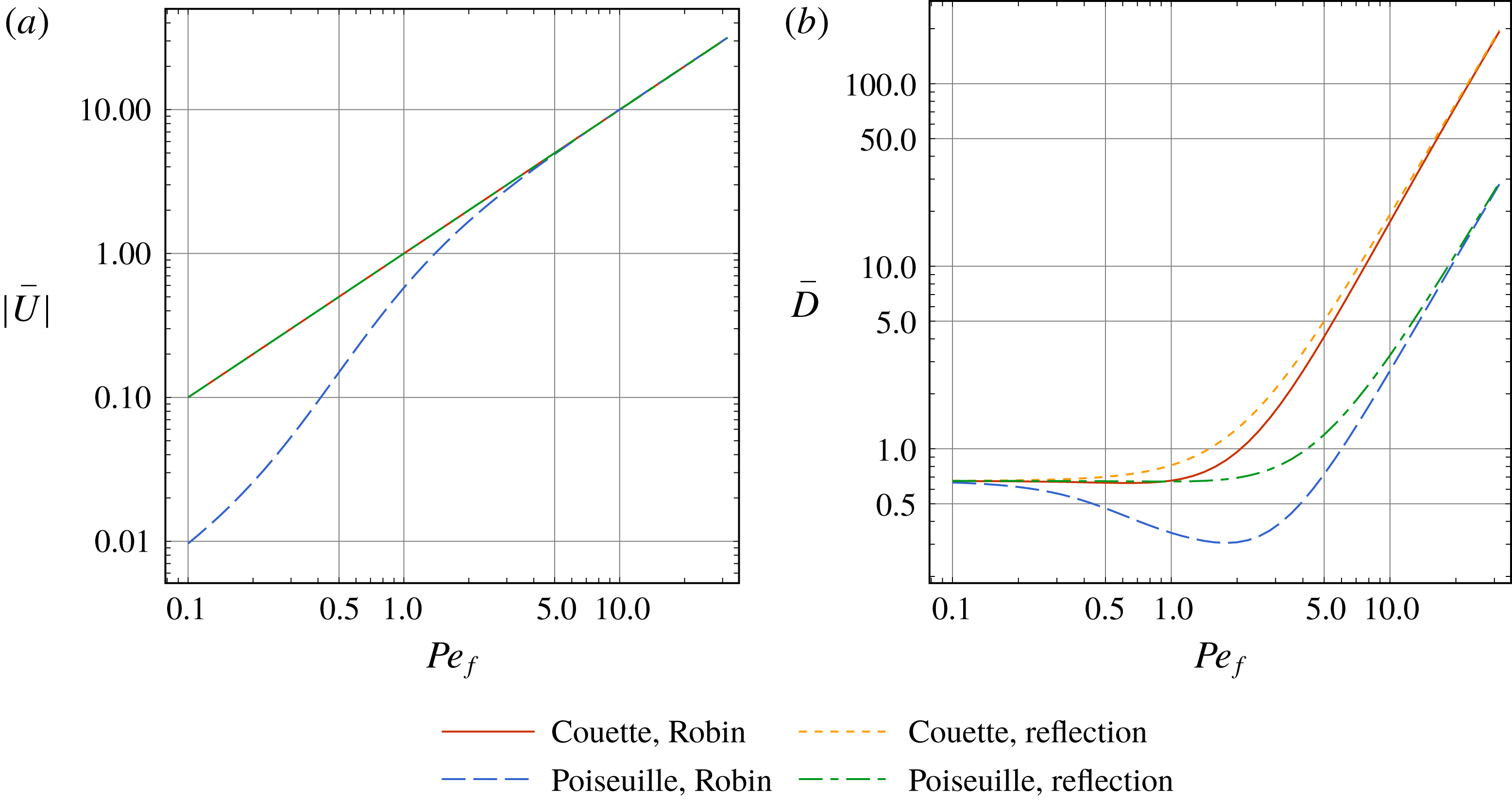
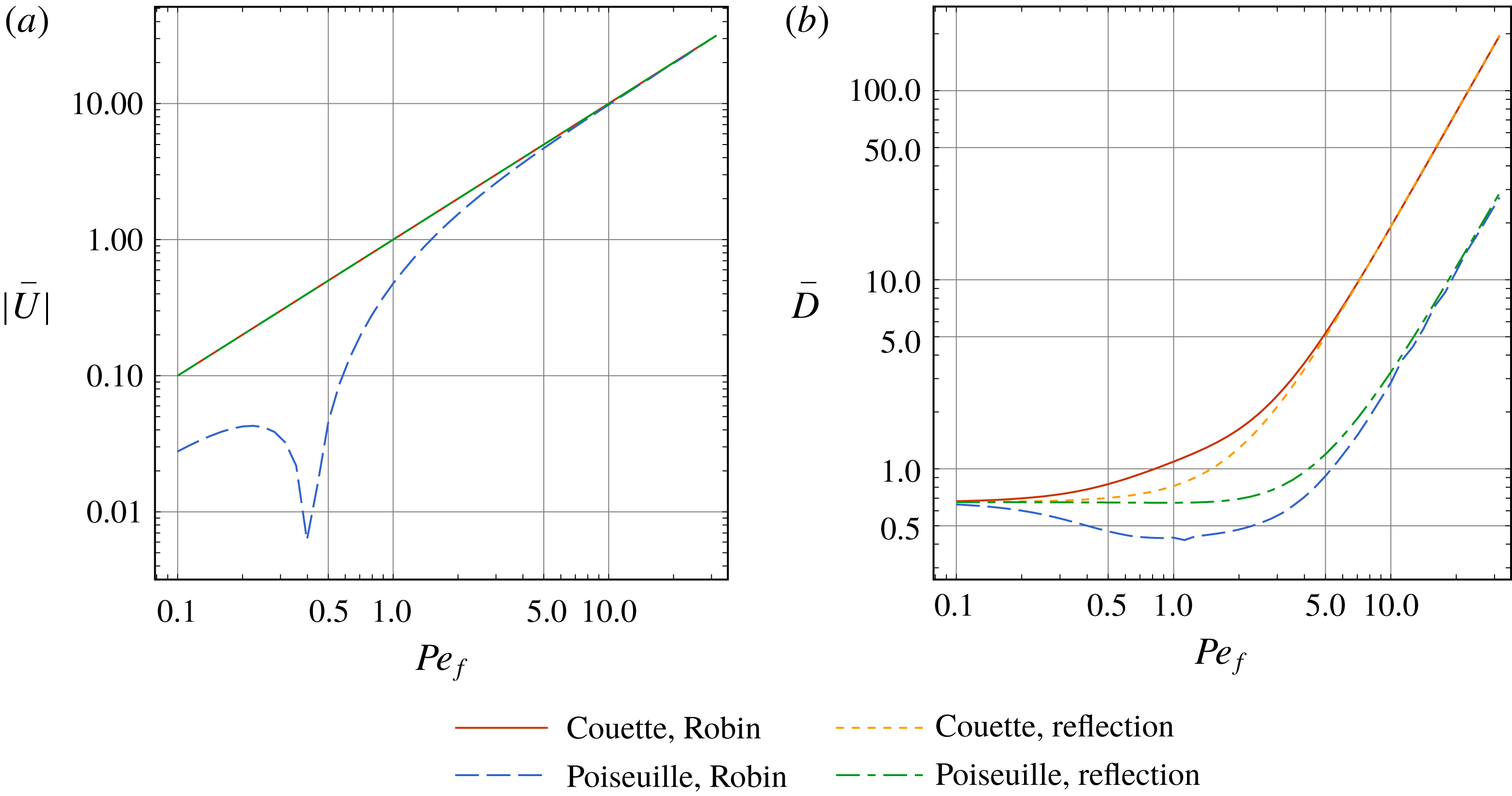
Figure 6(a) shows the difference of advection velocity $\bar{U}$ between the two studied cases, as well as between the boundary conditions. For the reflection boundary condition (2.14), the local distribution $P_{0}^{\infty }$ and the extended distribution $P_{E0}^{\infty }$ are uniform for the case of spherical particles. Thus the result of the integration (B 9) for extended advection velocity $\overline{U_{E}}$ is exactly equal to the flow Péclet number $\mathit{Pe}_{f}$ , i.e. the dimensionless transverse mean velocity. Through the relationship (B 10), we also have

(6.12) $$\begin{eqnarray}\bar{U}=\overline{U_{E}}=\mathit{Pe}_{f}.\end{eqnarray}$$

For the Robin boundary condition (2.13), the advection velocity (4.19) for the Couette flow is also equal to $\mathit{Pe}_{f}$ , due to the symmetric property (6.5). However, the symmetric structure (6.6) of the plane Poiseuille flow is different from that of the Couette flow. When $\mathit{Pe}_{f}$ is small (e.g. $\mathit{Pe}_{f}<1$ ), the advection velocity $\bar{U}$ (4.19) is much smaller than $\mathit{Pe}_{f}$ . Note that low velocity regions of the plane Poiseuille flow are near the walls, where the active particles accumulate. Besides, there are slightly more accumulated particles swimming upstream ( $\unicode[STIX]{x03C0}<\unicode[STIX]{x1D703}<2\unicode[STIX]{x03C0}$ ) than those swimming downstream ( $0<\unicode[STIX]{x1D703}<\unicode[STIX]{x03C0}$ ), referring to the nematic alignments in figure 3(d). Thus the total advection velocity is smaller than the mean velocity $\mathit{Pe}_{f}$ . When $\mathit{Pe}_{f}$ is large, the wall accumulation is hindered by the rapid rotation of particles, as shown in figure 5. The advection effect is dominant in the dispersion process, and the advection velocity $\bar{U}$ increases to $\mathit{Pe}_{f}$ .

Figure 6.

(a) Advection velocity $\bar{U}$ obtained by (4.19) and (B 9), (b) dispersivity $\bar{D}$ obtained by (4.37) and (B 17), as a function of the flow Péclet number $\mathit{Pe}_{f}$ , for the Couette flow and the plane Poiseuille flow and the two types of boundary conditions. ‘Couette’ denotes the Couette flow, and ‘Poiseuille’ denotes the plane Poiseuille flow. ‘Robin’ denotes the Robin boundary condition (2.13), and ‘Reflection’ denotes the reflection boundary condition (2.14). The particles are spherical. In all cases, $\unicode[STIX]{x1D6FC}_{0}=0$ , $\mathit{Pe}_{s}=1$ , $\unicode[STIX]{x1D6EC}=1/6$ .

Figure 6(b) shows that the overall dispersivity $\bar{D}$ (B 17) and (B 18) with reflection boundary condition (2.14) is larger than that (4.37) of the Robin form condition (2.13), for both of the studied flows. For spherical particles, the wall accumulation leads to a reduction of the dispersivity $\bar{D}$ , which is consistent with the numerical studies (Chilukuri et al. Reference Chilukuri, Collins and Underhill2015). The accumulation of active particles tends to weaken the whole dispersion as a global macrotransport process. When the flow Péclet number $\mathit{Pe}_{f}$ is large (e.g. $\mathit{Pe}_{f}\geqslant 10$ ), the difference in dispersivity $\bar{D}$ between these two types of boundary conditions disappears. The advection effect is obviously dominant in the dispersion process. Thus the scale of increased dispersivity is $\bar{D}\sim \mathit{Pe}_{f}^{2}$ , the same as in a dispersion process of passive particles (Aris Reference Aris1956; Barton Reference Barton1983).

The reasons for the reduction of dispersivity under the Robin condition in these two studied flows are different. Note both the advection effect caused by the flow and the swimming effect by the active particles exist during the dispersion process. For the Couette flow, the wall accumulation of particles can enhance the advection effect, because the relative velocity of the flow at the back wall ( $z=1$ ) to the flow at the front wall ( $z=0$ ) is larger. However, the nematic alignments of particles near the walls can weaken the swimming effect, because the accumulated particles mainly swim towards the wall, as shown in figure 3(a,b). However, under the reflection boundary condition, the particles swim freely. When the flow Péclet number $\mathit{Pe}_{f}$ is small, the swimming effect is dominant, and the overall effect by the Robin condition reduces the dispersivity.

For the plane Poiseuille flow, both the advection effect and the swimming effect are reduced under the Robin condition. The reduction of the swimming effect by the nematic alignments of particles is similar to the case with the Couette flow. However, the result of the wall accumulation on the advection effect is different. As there is no relative velocity between the walls ( $z=0,1$ ), the advection effect is dominated by the velocity difference of the flow between at the walls and along the centreline. Therefore, the wall accumulation (also a centreline depletion (Rusconi, Guasto & Stocker Reference Rusconi, Guasto and Stocker2014)) reduces the tendency of the particles to separate from each other. When the flow Péclet number $\mathit{Pe}_{f}$ is small, $\bar{D}$ decreases even more, with a downward trend in $\mathit{Pe}_{f}$ , consistent with the result of Chilukuri et al. (Reference Chilukuri, Collins and Underhill2015).

In addition, the dispersivity $\bar{D}$ in the plane Poiseuille flow is much smaller than that in the Couette flow for both types of boundary conditions, even in the advection-dominated regime with large $\mathit{Pe}_{f}$ . The reason lies in the difference between the velocity profiles. Unlike the uniform shear rate of the Couette flow across the channel, the high shear-rate regions of the plane Poiseuille flow, which can considerably increase the dispersivity, are only near the channel walls.

7.1 Local distribution $P_{0}^{\infty }(z,\unicode[STIX]{x1D703})$

7.1.1 The Robin boundary condition

For the case of the Robin boundary condition, the solution of $P_{0}^{\infty }(z,\unicode[STIX]{x1D703})$ is constructed through (4.7) and (4.16). The series expansion is verified with the numerical result of Nili et al. (Reference Nili, Kheyri, Abazari, Fahimniya and Naji2017), see appendix A. Parameters are kept the same as those of spherical particles in § 6.1.

The wall-normal polarization structure of the local distribution $P_{0}^{\infty }(z,\unicode[STIX]{x1D703})$ leads to the wall accumulation, as shown in figure 7. Like the case of the spherical particles in figure 3, external flows lead to the streamwise changes in polarization (Nili et al. Reference Nili, Kheyri, Abazari, Fahimniya and Naji2017). In the case with a low flow Péclet number $\mathit{Pe}_{f}$ , shown in figures 7(a,b) and 8(a,b), the swimming effect is dominant, with strong wall-normal polarization.

Figure 7.

Density plot of local distributions $P_{0}^{\infty }(z,\unicode[STIX]{x1D703})$ (4.7) and (4.16) of rod-like active particles in the two studied cases with various flow Péclet numbers $\mathit{Pe}_{f}$ . The boundary condition is in the Robin form (2.20). (a,c,e) Couette flow; (b,d,f) plane Poiseuille flow. (a,b)  $\mathit{Pe}_{f}=0.1$ ; (c,d) $\mathit{Pe}_{f}=1$ ; (e,f)  $\mathit{Pe}_{f}=10$ . In all cases, $\unicode[STIX]{x1D6FC}_{0}=1$ , $\mathit{Pe}_{s}=1$ , $\unicode[STIX]{x1D6EC}=1/6$ .

However, the streamwise nematic alignments (Ezhilan & Saintillan Reference Ezhilan and Saintillan2015) in the case of rod-like particles are much stronger than those of spherical particles, when the flow Péclet number $\mathit{Pe}_{f}$ is large, as depicted in figure 7(e,f). There are even bimodal distributions (Nili et al. Reference Nili, Kheyri, Abazari, Fahimniya and Naji2017) of swimming direction near wall regions. Because the angular velocity $\unicode[STIX]{x1D6FA}$ of rod-like particles (6.2) and (6.4) is affected not only by the ambient vorticity (2.11) but also by the strain tensor, rod-like particles have to align with the global streamlines of the imposed flow (i.e.  $\unicode[STIX]{x1D703}=\unicode[STIX]{x03C0}/2,\,3\unicode[STIX]{x03C0}/2$ ). As discussed by Nili et al. (Reference Nili, Kheyri, Abazari, Fahimniya and Naji2017) for the Couette flow and by Ezhilan & Saintillan (Reference Ezhilan and Saintillan2015) for the plane Poiseuille flow, the nematic alignments and bimodal distributions of swimming direction near wall regions are strengthened with high $\mathit{Pe}_{f}$ .

The streamwise nematic alignments and bimodal distributions can be seen more clearly by the local velocity fields $\boldsymbol{u}$ (defined in (6.10)) in the cross-section $Oz\unicode[STIX]{x1D703}$ , as shown in figure 8. Unlike the case of spherical particles, the angular velocity $\unicode[STIX]{x1D6FA}$ by the imposed flow $U(z)$ is dependent on both $\unicode[STIX]{x1D703}$ and $z$ . The global streamlines of the imposed flow ( $\unicode[STIX]{x1D703}=\unicode[STIX]{x03C0}/2,\,3\unicode[STIX]{x03C0}/2$ ) are singular, and there is no closed orbit in the middle of the channel (Zöttl & Stark Reference Zöttl and Stark2013). Thus all the particles will move to the walls or the singular lines, where the swimming flux is balanced by the diffusion flux.

Figure 8.

Local velocity vector $\boldsymbol{u}$ (6.10) fields for rod-like particles in the local space $\boldsymbol{q}=(z,\unicode[STIX]{x1D703})$ , with various flow Péclet numbers $\mathit{Pe}_{f}$ . (a,c,e) Couette flow; (b,d,f) plane Poiseuille flow. (a,b)  $\mathit{Pe}_{f}=0.1$ ; (c,d)  $\mathit{Pe}_{f}=1$ ; (e,f)  $\mathit{Pe}_{f}=10$ . Red lines are streamlines (regions near singular lines $\unicode[STIX]{x1D703}=\unicode[STIX]{x03C0}/2,\,3\unicode[STIX]{x03C0}/2$ are excluded).

7.1.2 The reflection boundary condition

For spherical particles, the local distribution is uniform for the reflection boundary condition. But for the rod-like particles, the nematic alignments and bimodal distributions, as shown in figure 7 for the Robin boundary condition, also exist under the reflection condition, though the wall accumulation is weak.

As depicted in figure 9, the streamwise nematic alignments of the local distribution are also strong for the reflection boundary condition, when the flow Péclet number $\mathit{Pe}_{f}$ is large (figure 9(e,f)). As discussed in § 7.1.1, rod-like particles have to align with the flow. When $\mathit{Pe}_{f}$ is small, the swimming effect is dominant. Thus the local distribution is nearly uniform, like in the case of spherical particles (§ 6.1.1), as shown in figure 9(c,d). There is no wall-normal polarization structure for the reflection boundary condition. Namely, no accumulation near points $(0,\unicode[STIX]{x03C0})$ and $(1,0)$ .

Figure 9.

Density plot of local distributions $P_{0}^{\infty }(z,\unicode[STIX]{x1D703})$ of rod-like active particles in the two studied cases with various flow Péclet numbers $\mathit{Pe}_{f}$ . The solution is obtained by the series expansion (B 7) and (B 8) for the reflection boundary condition (2.21). (a,c,e) extended Couette flow; (b,d,f) extended plane Poiseuille flow. (a,b)  $\mathit{Pe}_{f}=0.1$ ; (c,d)  $\mathit{Pe}_{f}=1$ ; (e,f)  $\mathit{Pe}_{f}=10$ . In all cases, $\unicode[STIX]{x1D6FC}_{0}=1$ , $\mathit{Pe}_{s}=1$ , $\unicode[STIX]{x1D6EC}=1/6$ .

The nematic alignment structures of the local distributions can be further understood by the field of the extended velocity vector

(7.3) $$\begin{eqnarray}\boldsymbol{u}_{E}=(\mathit{Pe}_{s}\cos \unicode[STIX]{x1D703},\unicode[STIX]{x1D6FA}_{E}(z,\unicode[STIX]{x1D703})).\end{eqnarray}$$

In fact, $\boldsymbol{u}_{E}$ can be obtained by reflecting the velocity vector $\boldsymbol{u}$ , in figure 8. Here we just show the case with flow Péclet number $\mathit{Pe}_{f}=1$ , as depicted in figure 10. Unlike the Robin condition, the boundary condition for the extended local distribution in the $z$ direction has been changed to periodic conditions (5.6) and (5.7). Thus rod-like particles only accumulate near the singular lines $\unicode[STIX]{x1D703}=\unicode[STIX]{x03C0}/2,\,3\unicode[STIX]{x03C0}/2$ , i.e. the direction of the global streamlines of the flow. To balance the diffusion flux, particles finally accumulate in the regions with local streamlines towards the singular lines, which accounts for the array patterned on the local distribution, as shown in figure 9(c,d).

Figure 10.

Extended local velocity vector $\boldsymbol{u}_{E}$ (7.3) fields for rod-like particles in the extended cross-section $\boldsymbol{q}=(z,\unicode[STIX]{x1D703})$ , reflected according to the local velocity field in figure 8(c,d). The flow Péclet number $\mathit{Pe}_{f}=1$ . (a) Couette flow; (b) plane Poiseuille flow. Red lines are streamlines.

7.1.3 Orientation-space mean PDF

Above results focus on the nematic alignments of local distribution $P_{0}^{\infty }(z,\unicode[STIX]{x1D703})$ . The wall-normal polarization structure of the local distribution leads to the wall accumulation, which can be shown more clearly by the orientation-space mean PDF $\langle P_{0}^{\infty }\rangle _{O}$ defined by (6.11), depicted in figure 11.

Figure 11.

Orientation-space mean PDF $\langle P_{0}^{\infty }\rangle _{O}$ (6.11) of rod-like particles with various flow Péclet numbers $\mathit{Pe}_{f}$ , (a) for the Robin boundary condition (2.20); (b) for the reflection boundary condition (2.21). ‘Couette’ denotes the Couette flow, and ‘Poiseuille’ denotes the plane Poiseuille flow. In all cases, $\unicode[STIX]{x1D6FC}_{0}=1$ , $\mathit{Pe}_{s}=1$ , $\unicode[STIX]{x1D6EC}=1/6$ .

For the Robin boundary condition (2.13) and (2.20), the wall accumulation is obvious when the flow Péclet number $\mathit{Pe}_{f}$ is small, which agrees with previous results (Ezhilan & Saintillan Reference Ezhilan and Saintillan2015; Nili et al. Reference Nili, Kheyri, Abazari, Fahimniya and Naji2017). Like the case of the spherical particles as shown in figure 5, the accumulation is suppressed by the large shear rate of global velocity (large $\mathit{Pe}_{f}$ ). This is due to the strong shear alignments. The reduction is stronger with the plane Poiseuille flow than the Couette flow, because the varied shear rate of the plane Poiseuille flow across the channel is much larger near the boundaries.

However, for the reflection boundary condition (2.14), there is no obvious wall accumulation. Unlike with the spherical particles, the orientation-space mean PDF is not uniform. Instead, the imposed global flow can enhance the variation of PDF of particles in the transverse direction, though the variations are still much smaller than those under the Robin boundary condition. As discussed in § 7.1.2, there is no wall-normal polarization structure associated with the reflection boundary condition. Thus the orientation-space mean PDF is nearly uniform. Furthermore, the periodic conditions (5.6) and (5.7) for the extended local distribution lead to a periodic extended velocity vector $\boldsymbol{u}_{E}$ field, as depicted in figure 10. The small variation of PDF with $z$ is to balance the diffusion flux with nematic alignments by the imposed flows.

Figure 12.

(a) Absolute value of advection velocity $|\bar{U}|$ obtained by (4.19) and (B 9), (b) Taylor dispersivity $\bar{D}$ obtained by (4.37) and (B 17), as a function of the flow Péclet number $\mathit{Pe}_{f}$ , for the two flows and the two types of boundary conditions. ‘Couette’ denotes the Couette flow, and ‘Poiseuille’ denotes the plane Poiseuille flow. ‘Robin’ denotes the Robin boundary condition (2.13), and ‘Reflection’ denotes the reflection boundary condition (2.14). The particles are rod-like. In all cases, $\unicode[STIX]{x1D6FC}_{0}=1$ , $\mathit{Pe}_{s}=1$ , $\unicode[STIX]{x1D6EC}=1/6$ .

7.2 Overall advection velocity $\bar{U}$ and dispersivity $\bar{D}$

For spherical particles, the accumulation under the Robin boundary condition leads to smaller dispersivity than that under the reflection condition, for both the Couette flow and the plane Poiseuille flow. This is not the case for rod-like particles. Here we also describe the influence of boundary conditions on the dispersion properties.

Figure 12(a) shows the difference of advection velocity $\bar{U}$ between the flows, as well as between the boundary conditions, similar to the case of spherical particles in figure 6(a). For the Robin boundary condition, due to the symmetric property (6.5a,b ) of the Couette flow, the advection velocity $\bar{U}$ (4.19) is equal to the flow Péclet number $\mathit{Pe}_{f}$ . However, for the plane Poiseuille flow, the variation of $\bar{U}$ in $\mathit{Pe}_{f}$ is different. When $\mathit{Pe}_{f}$ is small (e.g. $\mathit{Pe}_{f}<1$ ), the advection velocity $\bar{U}$ is much smaller and even becomes negative. The reasons are: first, the velocities of the accumulated regions are low, which reduce $\bar{U}$ , as discussed in § 6.2 for the spherical particles; second, the nematic alignments of rod-like particles by the imposed flow are so strong that the accumulated active particles on both channel walls mainly swim in the opposite direction of the flow ( $\unicode[STIX]{x1D703}=3\unicode[STIX]{x03C0}/2$ ), see figure 7(d). Thus $\bar{U}$ becomes negative. When $\mathit{Pe}_{f}$ is large, the wall accumulation is hindered by the strong shear alignments, see figure 11. The advection effect is dominant. As a result, $\bar{U}$ approaches to $\mathit{Pe}_{f}$ , as with spherical particles.

For the reflection boundary condition, the advection velocity $\bar{U}$ is almost equal to the flow Péclet number $\mathit{Pe}_{f}$ , for both flows. However, unlike that with spherical particles, the local distribution for rod-like particles is not uniform. In fact, the advection velocity $\bar{U}$ is not exactly equal to $\mathit{Pe}_{f}$ , with a pretty small deviation. When $\mathit{Pe}_{f}$ is small, the local distribution is nearly uniform, as depicted in figures 7(a,b) and 11(b). Thus the integration (B 9) for the extended advection velocity $\overline{U_{E}}$ is close to $\mathit{Pe}_{f}$ . When $\mathit{Pe}_{f}$ is large, the advection effect is dominant. In this way, $\bar{U}$ approaches $\mathit{Pe}_{f}$ and the small deviation further decreases.

For the plane Poiseuille flow, figure 12(b) shows that the dispersivity $\bar{D}$  (B 17) and (B 18) under the reflection boundary condition (2.14) is still larger than that (4.37) under the Robin form condition (2.13), similar to the case of spherical particles. However, for the Couette flow, dispersivity under the Robin condition is larger, when the flow Péclet number is small ( $\mathit{Pe}_{f}\sim 1$ ). As discussed in § 6.2, the wall accumulation of particles can enhance the advection effect in the dispersion process, since the relative velocities of the Couette flow between the wall regions are large. Unlike the spherical particles, rod-like particles accumulated at the back wall mainly swim in the same direction of the flow ( $\unicode[STIX]{x1D703}=\unicode[STIX]{x03C0}/2$ ), see figure 7(c), while at the front wall, they swim in the opposite direction $(\unicode[STIX]{x1D703}=3\unicode[STIX]{x03C0}/2)$ . Thus the nematic alignments of rod-like particles by shear can enhance the swimming effect. Therefore, the overall effects lead to an enhanced global dispersion process.

For the plane Poiseuille flow, the nematic alignments by shear are also strong. However, the accumulated active particles on both channel walls mainly swim in the same direction, opposite to the flow direction ( $\unicode[STIX]{x1D703}=3\unicode[STIX]{x03C0}/2$ ). Therefore, the nematic alignments cannot strengthen the swimming effects in the dispersion process like the case of the Couette flow. Additionally, in the advection-dominated regime with large $\mathit{Pe}_{f}$ (e.g. $\mathit{Pe}_{f}\geqslant 5$ ), the flow velocity is much larger than the swimming speed. Thus the scales of increased dispersivity with $\mathit{Pe}_{f}$ for both flows and boundary conditions are the same, as discussed in § 6.2 for spherical particles.