



%20--%3e%3c!DOCTYPE%20svg%20PUBLIC%20'-//W3C//DTD%20SVG%201.0//EN'%20'http://www.w3.org/TR/2001/REC-SVG-20010904/DTD/svg10.dtd'%3e%3csvg%20version='1.0'%20id='Layer_1'%20xmlns='http://www.w3.org/2000/svg'%20xmlns:xlink='http://www.w3.org/1999/xlink'%20x='0px'%20y='0px'%20width='64px'%20height='64px'%20viewBox='5.5%20-3.5%2064%2064'%20enable-background='new%205.5%20-3.5%2064%2064'%20xml:space='preserve'%3e%3cg%3e%3ccircle%20fill='%23FFFFFF'%20fill-opacity='0'%20cx='37.785'%20cy='28.501'%20r='28.836'/%3e%3cpath%20fill='%23595959'%20d='M37.441-3.5c8.951,0,16.572,3.125,22.857,9.372c3.008,3.009,5.295,6.448,6.857,10.314%20c1.561,3.867,2.344,7.971,2.344,12.314c0,4.381-0.773,8.486-2.314,12.313c-1.543,3.828-3.82,7.21-6.828,10.143%20c-3.123,3.085-6.666,5.448-10.629,7.086c-3.961,1.638-8.057,2.457-12.285,2.457s-8.276-0.808-12.143-2.429%20c-3.866-1.618-7.333-3.961-10.4-7.027c-3.067-3.066-5.4-6.524-7-10.372S5.5,32.767,5.5,28.5c0-4.229,0.809-8.295,2.428-12.2%20c1.619-3.905,3.972-7.4,7.057-10.486C21.08-0.394,28.565-3.5,37.441-3.5z%20M37.557,2.272c-7.314,0-13.467,2.553-18.458,7.657%20c-2.515,2.553-4.448,5.419-5.8,8.6c-1.354,3.181-2.029,6.505-2.029,9.972c0,3.429,0.675,6.734,2.029,9.913%20c1.353,3.183,3.285,6.021,5.8,8.516c2.514,2.496,5.351,4.399,8.515,5.715c3.161,1.314,6.476,1.971,9.943,1.971%20c3.428,0,6.75-0.665,9.973-1.999c3.219-1.335,6.121-3.257,8.713-5.771c4.99-4.876,7.484-10.99,7.484-18.344%20c0-3.543-0.648-6.895-1.943-10.057c-1.293-3.162-3.18-5.98-5.654-8.458C50.984,4.844,44.795,2.272,37.557,2.272z%20M37.156,23.187%20l-4.287,2.229c-0.458-0.951-1.019-1.619-1.685-2c-0.667-0.38-1.286-0.571-1.858-0.571c-2.856,0-4.286,1.885-4.286,5.657%20c0,1.714,0.362,3.084,1.085,4.113c0.724,1.029,1.791,1.544,3.201,1.544c1.867,0,3.181-0.915,3.944-2.743l3.942,2%20c-0.838,1.563-2,2.791-3.486,3.686c-1.484,0.896-3.123,1.343-4.914,1.343c-2.857,0-5.163-0.875-6.915-2.629%20c-1.752-1.752-2.628-4.19-2.628-7.313c0-3.048,0.886-5.466,2.657-7.257c1.771-1.79,4.009-2.686,6.715-2.686%20C32.604,18.558,35.441,20.101,37.156,23.187z%20M55.613,23.187l-4.229,2.229c-0.457-0.951-1.02-1.619-1.686-2%20c-0.668-0.38-1.307-0.571-1.914-0.571c-2.857,0-4.287,1.885-4.287,5.657c0,1.714,0.363,3.084,1.086,4.113%20c0.723,1.029,1.789,1.544,3.201,1.544c1.865,0,3.18-0.915,3.941-2.743l4,2c-0.875,1.563-2.057,2.791-3.541,3.686%20c-1.486,0.896-3.105,1.343-4.857,1.343c-2.896,0-5.209-0.875-6.941-2.629c-1.736-1.752-2.602-4.19-2.602-7.313%20c0-3.048,0.885-5.466,2.658-7.257c1.77-1.79,4.008-2.686,6.713-2.686C51.117,18.558,53.938,20.101,55.613,23.187z'/%3e%3c/g%3e%3c/svg%3e)
%20--%3e%3c!DOCTYPE%20svg%20PUBLIC%20'-//W3C//DTD%20SVG%201.0//EN'%20'http://www.w3.org/TR/2001/REC-SVG-20010904/DTD/svg10.dtd'%3e%3csvg%20version='1.0'%20id='Layer_1'%20xmlns='http://www.w3.org/2000/svg'%20xmlns:xlink='http://www.w3.org/1999/xlink'%20x='0px'%20y='0px'%20width='64px'%20height='64px'%20viewBox='5.5%20-3.5%2064%2064'%20enable-background='new%205.5%20-3.5%2064%2064'%20xml:space='preserve'%3e%3cg%3e%3ccircle%20fill='%23FFFFFF'%20fill-opacity='0'%20cx='37.637'%20cy='28.806'%20r='28.276'/%3e%3cg%3e%3cpath%20fill='%23595959'%20d='M37.443-3.5c8.988,0,16.57,3.085,22.742,9.257C66.393,11.967,69.5,19.548,69.5,28.5c0,8.991-3.049,16.476-9.145,22.456%20C53.879,57.319,46.242,60.5,37.443,60.5c-8.649,0-16.153-3.144-22.514-9.43C8.644,44.784,5.5,37.262,5.5,28.5%20c0-8.761,3.144-16.342,9.429-22.742C21.101-0.415,28.604-3.5,37.443-3.5z%20M37.557,2.272c-7.276,0-13.428,2.553-18.457,7.657%20c-5.22,5.334-7.829,11.525-7.829,18.572c0,7.086,2.59,13.22,7.77,18.398c5.181,5.182,11.352,7.771,18.514,7.771%20c7.123,0,13.334-2.607,18.629-7.828c5.029-4.838,7.543-10.952,7.543-18.343c0-7.276-2.553-13.465-7.656-18.571%20C50.967,4.824,44.795,2.272,37.557,2.272z%20M46.129,20.557v13.085h-3.656v15.542h-9.944V33.643h-3.656V20.557%20c0-0.572,0.2-1.057,0.599-1.457c0.401-0.399,0.887-0.6,1.457-0.6h13.144c0.533,0,1.01,0.2,1.428,0.6%20C45.918,19.5,46.129,19.986,46.129,20.557z%20M33.042,12.329c0-3.008,1.485-4.514,4.458-4.514s4.457,1.504,4.457,4.514%20c0,2.971-1.486,4.457-4.457,4.457S33.042,15.3,33.042,12.329z'/%3e%3c/g%3e%3c/g%3e%3c/svg%3e)
1. Introduction
The lattice Boltzmann method (LBM) models fluid flow using a fully discrete kinetic system of designer particles with discrete velocities  $\boldsymbol {c}_i$, fitting into a regular space-filling lattice. In the LBM, the kinetic evolution equation for the populations
 $f_i(\boldsymbol {x},t)$ follows a simple algorithm of ‘stream along links
 $\boldsymbol {c}_i$ and collide at the nodes
 $\boldsymbol {x}$ in discrete time
 $t$’. Since its inception (Higuera & Jiménez Reference Higuera and Jiménez1989; Higuera & Succi Reference Higuera and Succi1989), LBM has evolved into a versatile tool for the simulation of complex flows, including but not limited to turbulent flows (Dorschner, Chikatamarla & Karlin Reference Dorschner, Chikatamarla and Karlin2016, Reference Dorschner, Chikatamarla and Karlin2017), biological flows (Falcucci et al. Reference Falcucci, Amati, Fanelli, Krastev, Polverino, Porfiri and Succi2021), compressible flows (Xu & Sagaut Reference Xu and Sagaut2013; Frapolli, Chikatamarla & Karlin Reference Frapolli, Chikatamarla and Karlin2016; Dorschner, Bösch & Karlin Reference Dorschner, Bösch and Karlin2018; Lin & Luo Reference Lin and Luo2018; Yang, West & Harris Reference Yang, West and Harris2018), multiphase flows (Mazloomi, Chikatamarla & Karlin Reference Mazloomi, Chikatamarla and Karlin2015, Reference Mazloomi, Chikatamarla and Karlin2017; Wöhrwag et al. Reference Wöhrwag, Semprebon, Mazloomi, Karlin and Kusumaatmaja2018), rarefied gas (Shan, Yuan & Chen Reference Shan, Yuan and Chen2006) and nanoflow (Montessori et al. Reference Montessori, Prestininzi, Rocca, Falcucci, Succi and Kaxiras2016; Montemore et al. Reference Montemore, Montessori, Succi, Barroo, Falcucci, Bell and Kaxiras2017). While the majority of the LBM development concerns single-component fluids, the case of mixtures, and especially of reactive mixtures, remains an active area of research (Yan et al. Reference Yan, Xu, Zhang, Ying and Li2013; Feng, Tayyab & Boivin Reference Feng, Tayyab and Boivin2018; Hosseini, Darabiha & Thévenin Reference Hosseini, Darabiha and Thévenin2018; Lin & Luo Reference Lin and Luo2018; Hosseini et al. Reference Hosseini, Safari, Darabiha, Thévenin and Krafczyk2019, Reference Hosseini, Abdelsamie, Darabiha and Thévenin2020; Tayyab et al. Reference Tayyab, Radisson, Almarcha, Denet and Boivin2020; Tayyab, Zhao & Boivin Reference Tayyab, Zhao and Boivin2021). Recently, in Sawant, Dorschner & Karlin (Reference Sawant, Dorschner and Karlin2021a), we revisited the LBM construction for a compressible multicomponent mixture, focusing on a thermodynamically consistent coupling between diffusion and momentum and energy transfer. The species kinetic equations recovered the Stefan–Maxwell diffusion with barodiffusion in the hydrodynamic limit. In addition, we also validated and derived from our kinetic model approximate diffusion models such as the Curtiss–Hirschfelder model and the generalized Fick model (Kee, Coltrin & Glarborg Reference Kee, Coltrin and Glarborg2003; Poinsot & Veynante Reference Poinsot and Veynante2005; Giovangigli Reference Giovangigli2012). A mean field was introduced for the lattice Boltzmann formulation of the mixture momentum and energy using a two-population lattice Boltzmann equation for the mixture. The mean-field approach consists of two lattice Boltzmann equations, one for the mixture density and momentum, and another for the energy with the help of a modification of the non-equilibrium fluxes. The two-population mixture LBM and the lattice Boltzmann scheme for the species kinetic equations were realized on the standard three-dimensional lattice. The resulting LBM provides a reduced description of the
 $M$-component mixture with
 $M+2$ tightly coupled lattice Boltzmann equations.
In this paper, we extend the two-population mixture LBM to reactive flows and show viability and accuracy for practical applications. To that end, we propose novel boundary conditions for walls as well as inlets and outlets. Furthermore, unlike previous realizations (Sawant et al. Reference Sawant, Dorschner and Karlin2021a; Sawant, Dorschner & Karlin Reference Sawant, Dorschner and Karlin2021b), we use the extended LBM (Saadat, Dorschner & Karlin Reference Saadat, Dorschner and Karlin2021a; Saadat et al. Reference Saadat, Hosseini, Dorschner and Karlin2021b) for the mean-field model. For validation, we start with simulations of a perfectly stirred reactor and a one-dimensional laminar flame. Subsequently, combustion of a lean hydrogen/air mixture in microtubes is simulated in two and three dimensions. A variety of different flame dynamics, such as the periodic ignition-extinction, stable symmetric V-shaped flames and asymmetric flames, are captured by the reactive LBM, and our simulations are in quantitative agreement with the direct numerical simulations (DNS) of Pizza et al. (Reference Pizza, Frouzakis, Mantzaras, Tomboulides and Boulouchos2008b, Reference Pizza, Frouzakis, Mantzaras, Tomboulides and Boulouchos2010).
The paper is structured as follows. We begin with a recap of the nomenclature and the kinetic system for the species in § 2. This section presents the discrete lattice Boltzmann equations for the reactive species and their implementation on the standard lattice. The section closes with a short discussion on time integration of the reaction mass source term. Next, we turn our attention to describing the mean-field approach for modelling the momentum and energy of the reactive mixture in § 3. Here, we discuss the adoption of the extended LBM for reactive flows, and present the realization on a standard lattice with the two-population approach. The section closes with a brief outline of the resultant macroscopic Navier–Stokes equations in the continuum limit, followed by validation with the perfectly stirred reactor and one-dimensional laminar flame. Having described completely the dynamics in bulk of the multicomponent fluid, we proceed to formulate the boundary conditions for the combined model in § 4. In § 4.2, we discuss the equivalent of a no-slip adiabatic boundary condition using the popular bounce-back method. This is followed by a technique to implement an isothermal wall based on the Tamm–Mott-Smith boundary condition in the lattice Boltzmann framework. Next, a realization for applying the inlet flux boundary condition is discussed in § 4.3. In § 4.4, a convective boundary condition, which can be used in conjunction with the characteristics-based boundary condition, is provided to approximate the species mass fractions at the outlet. With the resultant model, we compute the combustion of a premixed hydrogen/air mixture flowing through hot microtubes in § 5. Validation is performed in different regimes by changing the inlet velocity. The two-dimensional simulation exhibits rich flame dynamics by undergoing repetitive extinction and ignition, forming stable V-shaped flame and stable asymmetric flames. Finally, a three-dimensional open flame is computed in a microtube.
2. Lattice Boltzmann model for the species
2.1. Kinetic equations for the species
The nomenclature follows Sawant et al. (Reference Sawant, Dorschner and Karlin2021a). The composition of a reactive mixture of  $M$ components is described by the species densities
 $\rho _a$,
 $a=1,\ldots, M$, while the mixture density is
 \begin{equation} \rho=\sum_{a=1}^{M}\rho_a.\end{equation}
The rate of change of species densities due to reaction,  $\dot \rho _a^{r}$, satisfies mass conservation,
 \begin{equation} \sum_{a=1}^{M}\dot \rho_a^{r} = 0.\end{equation}
Introducing the mass fraction,  $Y_a={\rho _a}/{\rho }$, the molar mass of the mixture
 $m$ is given by
 ${m}^{-1}=\sum _{a=1}^M Y_a/m_a,$ where
 $m_a$ is the molar mass of the component
 $a$. The ideal gas equation of state provides a relation between the pressure
 $P$, the temperature
 $T$ and the composition
 \begin{equation} P=\rho R T,\end{equation}
where  $R={R_U}/{m}$ is the specific gas constant of the mixture, and
 $R_U$ is the universal gas constant. The pressure of an individual component is related to the pressure of the mixture through Dalton's law of partial pressures,
 $P_a=X_a P$, where the mole fraction is
 $X_a={m} Y_a /{m_a}$. Combined with the equation of state (2.3), the partial pressure takes the form
 $P_a=\rho _a R_a T$, where
 $R_a={R_U}/{m_a}$ is the specific gas constant of the component.
In the kinetic representation, each component is described by a set of populations  $f_{ai}$ corresponding to the discrete velocities
 $\boldsymbol {c}_i$,
 $i=0,\ldots, Q-1$. The species densities
 $\rho _a$ and the partial momenta
 $\rho _a \boldsymbol {u}_a$ are defined accordingly as
 \begin{gather} \rho_a= \sum_{i=0}^{Q-1}f_{ai}, \end{gather}
 \begin{gather}\rho_a \boldsymbol{u}_a= \sum_{i=0}^{Q-1} f_{ai}\boldsymbol{c}_i, \end{gather}
while partial momenta sum to the mixture momentum,
 \begin{equation} \rho\boldsymbol{u}=\sum_{a=1}^M\rho_a\boldsymbol{u}_a.\end{equation}
Following Sawant et al. (Reference Sawant, Dorschner and Karlin2021a,Reference Sawant, Dorschner and Karlinb), the kinetic equations for the species can be written as
 \begin{equation} \partial_t f_{ai} + \boldsymbol{c}_{i}\boldsymbol{\cdot}\boldsymbol{\nabla}f_{ai} = \sum_{b\ne a}^M \frac{PX_aX_b}{\mathcal{D}_{ab}} \left[ \left( \frac{f_{ai}^{eq}-f_{ai}}{\rho_a} \right) - \left( \frac{f_{bi}^{eq}-f^*_{bi}}{\rho_b} \right) \right]+ \dot f_{ai}^{r},\end{equation}
where  $\mathcal {D}_{ab}$ are Stefan–Maxwell binary diffusion coefficients, while the reaction source term satisfies the following conditions, consistent with (2.4):
 \begin{gather} \sum_{i=0}^{Q-1} \dot f_{ai}^{r}= \dot \rho_a^{r}, \end{gather}
 \begin{gather}\sum_{i=0}^{Q-1} \dot f_{ai}^{r}\boldsymbol{c}_i = \dot \rho_a^{r}\boldsymbol{u}. \end{gather}
We now proceed with specifying the equilibrium  $f_{ai}^{eq}$, the quasi-equilibrium
 $f^*_{ai}$ and the reaction source term
 $\dot f_{ai}^{r}$.
2.2. Standard lattice and product form
Kinetic model (2.7) is realized on the standard discrete velocity set  $D3Q27$, where
 $D=3$ stands for three dimensions and
 $Q=27$ is the number of discrete velocities,
 \begin{equation} \boldsymbol{c}_i=(c_{ix},c_{iy},c_{iz}),\quad c_{i\alpha}\in\{{-}1,0,1\}. \end{equation}
In order to specify the equilibrium  $f_{ai}^{eq}$, the quasi-equilibrium
 $f^*_{ai}$ and the reaction source term
 $\dot f_{ai}^{r}$ in (2.7), we first define a triplet of functions in two variables,
 $\xi _{\alpha }$ and
 $\mathcal {P}_{\alpha \alpha }$,
 \begin{gather} \varPsi_{0}(\xi_{\alpha},\mathcal{P}_{\alpha\alpha}) = 1 - \mathcal{P}_{\alpha\alpha}, \end{gather}
 \begin{gather}\varPsi_{1}(\xi_{\alpha},\mathcal{P}_{\alpha\alpha}) = \frac{\xi_{\alpha} + \mathcal{P}_{\alpha\alpha}}{2}, \end{gather}
 \begin{gather}\varPsi_{{-}1}(\xi_{\alpha},\mathcal{P}_{\alpha\alpha}) = \frac{-\xi_{\alpha} + \mathcal{P}_{\alpha\alpha}}{2}, \end{gather}
and consider a product form associated with the discrete velocities  $\boldsymbol {c}_i$ in (2.10),
 \begin{equation} \varPsi_i= \varPsi_{c_{ix}}(\xi_x,\mathcal{P}_{xx})\, \varPsi_{c_{iy}}(\xi_y,\mathcal{P}_{yy})\,\varPsi_{c_{iz}}(\xi_z,\mathcal{P}_{zz}). \end{equation}
All pertinent populations to be encountered in this paper will be determined by specifying the parameters  $\xi _\alpha$ and
 $\mathcal {P}_{\alpha \alpha }$ in the product form (2.14). To that end, the equilibrium and the quasi-equilibrium populations are found by setting
 \begin{gather} \xi_\alpha=u_\alpha, \end{gather}
 \begin{gather}\mathcal{P}_{\alpha \alpha}=R_aT+u_{\alpha}^2, \end{gather}
in the former cases, and
 \begin{gather} \xi_\alpha=u_{a\alpha}, \end{gather}
 \begin{gather}\mathcal{P}_{\alpha \alpha}=R_aT+u_{a\alpha}^2, \end{gather}
in the latter cases:
 \begin{gather} f_{ai}^{eq} = \rho_a\,\varPsi_{c_{ix}}(u_x,u_x^2+R_aT)\, \varPsi_{c_{iy}}(u_y,u_y^2+R_aT)\, \varPsi_{c_{iz}}(u_z,u_z^2+R_aT), \end{gather}
 \begin{gather}f_{ai}^{*} = \rho_a\,\varPsi_{c_{ix}}(u_{ax},u_{ax}^2+R_aT)\, \varPsi_{c_{iy}}(u_{ay},u_{ay}^2+R_aT)\, \varPsi_{c_{iz}}(u_{az},u_{az}^2+R_aT). \end{gather}
Reaction terms are specified with the product form (2.14) using the equilibrium parameters (2.16):
 \begin{equation} \dot f_{ai}^{r} = \dot \rho_a^{r}\, \varPsi_{c_{ix}}(u_{x},u_{x}^2+R_aT)\, \varPsi_{c_{iy}}(u_{y},u_{y}^2+R_aT)\, \varPsi_{c_{iz}}(u_{z},u_{z}^2+R_aT). \end{equation}
Analysis of the hydrodynamic limit of the kinetic model (2.7) follows the lines already presented in Sawant et al. (Reference Sawant, Dorschner and Karlin2021a). The balance equations for the densities of the species in the presence of the source term are found as follows:
 \begin{equation} \partial_t\rho_a={-}\boldsymbol{\nabla}\boldsymbol{\cdot}(\rho_a \boldsymbol{u})-\boldsymbol{\nabla}\boldsymbol{\cdot}(\rho_a \delta\boldsymbol{u}_a) + \dot \rho_a^{r},\end{equation}
where the diffusion velocities  $\delta \boldsymbol {u}_a=\boldsymbol {u}_a-\boldsymbol {u}$ satisfy the Stefan–Maxwell constitutive relation
 \begin{equation} P\,\boldsymbol{\nabla} X_a+(X_a-Y_a)\,\boldsymbol{\nabla} P=\sum_{b\ne a}^M \frac{PX_aX_b}{\mathcal{D}_{ab}}\,({\delta}\boldsymbol{u}_{b} - {\delta}\boldsymbol{u}_a ). \end{equation}
Summarizing, kinetic model (2.7) recovers both the Stefan–Maxwell law of diffusion and the composition change due to chemical reaction, as presented in (2.22).
2.3. Lattice Boltzmann equation for the species
Derivation of the lattice Boltzmann equation from the kinetic model (2.7) proceeds along the lines of the non-reactive case already presented in detail by Sawant et al. (Reference Sawant, Dorschner and Karlin2021a). Upon integration of (2.7) along the characteristics and application of the trapezoidal rule to all relaxation terms on the right-hand side apart from the reaction term, we arrive at a fully discrete lattice Boltzmann equation for the species:
 \begin{equation} f_{ai}(\boldsymbol{x}+\boldsymbol{c}_i \delta t, t+ \delta t) = f_{ai}(\boldsymbol{x},t)+ 2 \beta_a [f_{ai}^{eq}(\boldsymbol{x},t) - f_{ai}(\boldsymbol{x},t)] + \delta t (\beta_a-1)\,F_{ai}(\boldsymbol{x}, t) + R_{ai}^{r}. \end{equation}
Here,  $\delta t$ is the lattice time step, the equilibrium populations are provided by (2.19), and the relaxation parameters
 $\beta _a\in [0,1]$ are
 \begin{equation} \beta_a=\frac{\delta t}{2 \tau_a + \delta t}. \end{equation}
Their relation to the Stefan–Maxwell binary diffusion coefficients is found as follows. Introducing characteristic times
 \begin{equation} \tau_{ab}=\frac{mR_UT}{\mathcal{D}_{ab}m_a m_b}, \end{equation}
the relaxation times  $\tau _a$ in (2.25) are defined as
 \begin{equation} \frac{1}{\tau_a} = \sum_{b\ne a}^M \frac{Y_b}{\tau_{ab}}.\end{equation}
Furthermore, in (2.24), the quasi-equilibrium relaxation term  $F_{ai}$ is spelled out as
 \begin{equation} F_{ai} = Y_a \sum_{b\ne a}^M \frac{1}{\tau_{ab}}\,( f_{bi}^{eq}-f_{bi}^* ). \end{equation}
Here, the quasi-equilibrium populations  $f_{bi}^*$ are defined by the product form (2.20), subject to the parametrization
 \begin{gather} \xi_\alpha=u_{\alpha}+V_{b\alpha}, \end{gather}
 \begin{gather}\mathcal{P}_{\alpha \alpha}=R_bT+(u_{\alpha}+V_{b\alpha})^2, \end{gather}
where the second-order accurate diffusion velocity  $\boldsymbol {V}_b$ is the result of the lattice Boltzmann discretization of the kinetic equation, and is found by solving the
 $M\times M$ linear algebraic system for each spatial component:
 \begin{equation} \left( 1+ \frac{\delta t}{2 \tau_a}\right) {\boldsymbol{V}_{a}} - \frac{\delta t}{2} \sum_{b\ne a}^{M} \frac{1}{\tau_{ab}}\,Y_b {\boldsymbol{V}_{b}}=\boldsymbol{u}_{a}-\boldsymbol{u}. \end{equation}
The system (2.31) has been derived in Sawant et al. (Reference Sawant, Dorschner and Karlin2021a) and is not altered by the presence of the reaction. In our realization, we solve (2.31) with the Householder QR decomposition method from the Eigen library (Guennebaud & Jacob Reference Guennebaud and Jacob2010).
All the elements of the lattice Boltzmann equation (2.24) described so far are identical to those already present in the non-reactive case of Sawant et al. (Reference Sawant, Dorschner and Karlin2021a). Finally, the reaction term in (2.24) is represented by an integral over the characteristics,
 \begin{equation} {R_{ai}^{r}}=\delta t\int_{0}^{1}\dot f_{ai}^{r}(\boldsymbol{x}+\boldsymbol{c}_i s\,\delta t,t+s\,\delta t )\, {\rm d} s. \end{equation}
Taking into account the structure of the reaction term (2.21), we use a simple explicit approximation for the implicit term (2.32):
 \begin{equation} {R_{ai}^{r}}\approx\rho^{{-}1}f_{ai}^{eq}(\boldsymbol{x},t)\,\delta t\int_{0}^{1}\dot \rho_{a}^{r}(\boldsymbol{x},t+s\,\delta t)\, {\rm d} s. \end{equation}
Reaction rates  $\dot \rho _a^{r}$ are obtained from the open source chemical kinetics package Cantera (Goodwin et al. Reference Goodwin, Speth, Moffat and Weber2018) as a function of mixture internal energy
 $U$ and composition
 $\dot \rho _a^{r}=\dot \rho _a^{r}(U,\rho _1,\ldots,\rho _M)$. In order to mitigate the stiffness of the reaction rates for detailed reaction mechanisms, we introduce a time step
 $\delta t^{r} = {\delta t}/{l}$, where
 $l=1,2,\ldots$, and evaluate (2.33) by forward Euler in
 $l$ sub-steps,
 \begin{equation} R_{ai}^{r}\approx \rho^{{-}1}\,f_{ai}^{eq}(\boldsymbol{x},t)\left[ \delta t^{r}\sum_{s=0}^{l-1}\dot \rho_a^{r}( U(\boldsymbol{x},t),\rho_1(\boldsymbol{x},t+s\,\delta t^{r}),\ldots,\rho_M(\boldsymbol{x},t+s\,\delta t^{r}))\right].\end{equation}
Note that during sub-iterations, the energy remains fixed although the temperature changes, in general. In other words, at each grid point, sub-iterations implement a zero-dimensional perfectly stirred reactor. Execution time for sub-steps increases by about  $6\,\%$ for
 $l=2$ and by
 $15\,\%$ for
 $l=4$. In this paper, we use
 $l=2$, which is small enough that the integration error does not influence the flow solution but still reduces the computational complexity by roughly half due to the larger time step of the fluid solver,
 $\delta t = 2\,\delta t^r$.
Summarizing, the lattice Boltzmann system (2.24) delivers the extension of the species dynamics subject to the Stefan–Maxwell diffusion to the reactive mixtures. We now proceed with setting up the lattice Boltzmann equations for the mixture momentum and energy.
3. Lattice Boltzmann model of mixture momentum and energy
3.1. Double-population lattice Boltzmann equation
The mass-based specific internal energy  ${U}_{a}$ and enthalpy
 ${H}_{a}$ of the species are
 \begin{gather} {U}_{a}=U^0_a+\int_{T_0}^T{C}_{a,v}(T')\, {\rm d} T', \end{gather}
 \begin{gather}{H}_{a}=H^0_a+\int_{T_0}^T{C}_{a,p}(T')\, {\rm d} T', \end{gather}
where  $U^0_a$ and
 $H^0_a$ are the energy and the enthalpy of formation at the reference temperature
 $T_0$, respectively, while
 $C_{a,v}$ and
 $C_{a,p}$ are specific heats at constant volume and at constant pressure, satisfying the Mayer relation
 ${C}_{a,p}-{C}_{a,v}=R_{a}$. Consequently, the internal energy
 $\rho U$ and enthalpy
 $\rho H$ of the mixture are defined as
 \begin{gather} \rho U=\sum_{a=1}^M\rho_a U_a, \end{gather}
 \begin{gather}\rho H=\sum_{a=1}^M\rho_a H_a. \end{gather}
While the sensible heat was considered in the non-reactive case (Sawant et al. Reference Sawant, Dorschner and Karlin2021a), by taking into account the heat of formation, we immediately extend the model to reactive mixtures. As in Sawant et al. (Reference Sawant, Dorschner and Karlin2021a), we follow a two-population approach. One set of populations ( $f$-populations) is used to represent the density and the momentum of the mixture. Below, we refer to the
 $f$-populations as the momentum lattice. The locally conserved fields are the density and the momentum of the mixture,
 \begin{gather} \sum_{i=0}^{Q-1} f_i = \rho, \end{gather}
 \begin{gather}\sum_{i=0}^{Q-1} f_i \boldsymbol{c}_{i} = \rho \boldsymbol{u}. \end{gather}
Another set of populations ( $g$-populations), or the energy lattice, is used to represent the local conservation of the total energy of the mixture,
 \begin{gather} \sum_{i=0}^{Q-1} g_i = \rho E, \end{gather}
 \begin{gather}\rho E=\rho U + {\frac{\rho u^2}{2}}. \end{gather}
Since the mixture internal energy (3.3) depends on the composition, the species kinetic equations become coupled with the kinetic equations for the mixture to be introduced shortly. Conversely, the temperature is evaluated by solving the integral equation (cf. (3.1) and (3.3))
 \begin{equation} \sum_{a=1}^MY_a\left[U_a^0 + \int_{T_0}^T {C}_{a,v}(T')\, {\rm d} T'\right]=E-\frac{u^2}{2}. \end{equation}
The temperature evaluated by solving (3.9) is used as the input in the equation of state (2.3) elsewhere in the species lattice Boltzmann system. This furnishes a two-way coupling input between the species and the mixture kinetic systems.
Similar to Sawant et al. (Reference Sawant, Dorschner and Karlin2021a), the lattice Boltzmann equations for the momentum and for the energy lattice are patterned from the single-component developments and are realized on the  $D3Q27$ discrete velocity set. While the prototype single-component LBM used in Sawant et al. (Reference Sawant, Dorschner and Karlin2021a) was that of Saadat, Bösch & Karlin (Reference Saadat, Bösch and Karlin2019), here we take advantage of a more recent proposal by Saadat et al. (Reference Saadat, Dorschner and Karlin2021a). It is noted that while these single-component models are essentially equivalent, the recent formulation is more compact in its formulation and simpler in terms of implementation. Following the more recent proposal, the mixture lattice Boltzmann equations are written as
 \begin{gather} f_i(\boldsymbol{x}+\boldsymbol{c}_i\,\delta t,t+\delta t)- f_i(\boldsymbol{x},t)= \omega (f_i^{ex} -f_i), \end{gather}
 \begin{gather}g_i(\boldsymbol{x}+\boldsymbol{c}_i\,\delta t,t+ \delta t) - g_i(\boldsymbol{x},t)= \omega_1 (g_i^{eq} -g_i) + (\omega - \omega_1) (g_i^{*} -g_i), \end{gather}
where relaxation parameters  $\omega$ and
 $\omega _1$ are related to the mixture viscosity and thermal conductivity, and we proceed with specifying the pertinent populations in (3.10) and (3.11).
3.2. Extended equilibrium for the momentum lattice
The extended equilibrium populations  $f_i^{ex}$ in (3.10) are specified by the product form (2.14), with the parameters identified as
 ${\xi }_{\alpha }={u}_{\alpha }$ and
 $\mathcal {P}_{\alpha \alpha }=\mathcal {P}_{\alpha \alpha }^{ex}$:
 \begin{equation} f_{i}^{ex}=\rho\,\varPsi_{c_{ix}}(u_{x},\mathcal{P}_{xx}^{ex})\, \varPsi_{c_{iy}}(u_{y},\mathcal{P}_{yy}^{ex})\, \varPsi_{c_{iz}}(u_{z},\mathcal{P}_{zz}^{ex}), \end{equation}
where the extended parameter  $\mathcal {P}_{\alpha \alpha }^{ex}$ is
 \begin{equation} \mathcal{P}_{\alpha \alpha}^{ex} = \mathcal{P}_{\alpha \alpha}^{eq} + \delta t\left( \frac{2-\omega}{2\rho\omega}\right) \partial_\alpha (\rho u_\alpha (1 - 3 R T) - \rho u_\alpha^3), \end{equation}
while  $\mathcal {P}_{\alpha \alpha }^{eq}$, given by
 \begin{equation} \mathcal{P}_{\alpha \alpha}^{eq} = RT+u_\alpha^2,\end{equation}
corresponds to the conventional product-form equilibrium
 \begin{equation} f_{i}^{eq}=\rho\, \varPsi_{c_{ix}}(u_{x},\mathcal{P}_{xx}^{eq})\, \varPsi_{c_{iy}}(u_{y},\mathcal{P}_{yy}^{eq})\, \varPsi_{c_{iz}}(u_{z},\mathcal{P}_{zz}^{eq}).\end{equation}
The effect of extension, featured by the second term in (3.13), is to correct for the incomplete Galilean invariance of the standard  $D3Q27$ velocity set (2.10). With the original formulation of the mixture momentum lattice in Sawant et al. (Reference Sawant, Dorschner and Karlin2021a), a similar correction was achieved by augmenting (3.10) with an additional forcing term that required evaluation of second-order derivatives in space. In the present formulation, the correction of Galilean invariance is achieved by the extended equilibrium that requires evaluation of only a first-order derivative (cf. (3.13)), a more local operation.
3.3. Equilibrium and quasi-equilibrium of the energy lattice
Turning our attention to the energy lattice, the corresponding equilibrium and quasi-equilibrium populations in (3.11) are evaluated along the lines of Saadat et al. (Reference Saadat, Dorschner and Karlin2021a). Let us introduce linear operators  ${O}_\alpha$, acting on any smooth function
 $A(\boldsymbol {u},T)$ according to a rule
 \begin{equation} {O}_\alpha A= RT\,\frac{\partial A}{\partial u_\alpha} + u_\alpha A.\end{equation}
The equilibrium populations  $g_i^{eq}$ are specified with an operator version of the product form (2.14). To that end, we consider parameters
 ${\xi _\alpha }$ and
 $\mathcal {P}_{\alpha \alpha }$ as operator symbols:
 \begin{gather} \xi_\alpha = {O}_\alpha, \end{gather}
 \begin{gather}\mathcal{P}_{\alpha\alpha} = {O}_\alpha^2. \end{gather}
With the operators (3.17) and (3.18) substituted into the product form (2.14), the equilibrium populations  $g_i^{eq}$ are written compactly using the energy
 $E$ as the generating function:
 \begin{equation} g_i^{eq} = \rho\,\varPsi_{c_{ix}}({O}_x,{O}_x^2)\, \varPsi_{c_{iy}}({O}_y,{O}_y^2)\, \varPsi_{c_{iz}}({O}_z,{O}_z^2)\,E. \end{equation}
It is straightforward to verify by a direct computation that the equilibrium (3.19) satisfies the necessary conditions to recover the mixture energy equation as in Sawant et al. (Reference Sawant, Dorschner and Karlin2021a), namely, the equilibrium energy flux  $\boldsymbol {q}^{eq}$ and the flux thereof
 $\boldsymbol {R}^{eq}$:
 \begin{gather} \boldsymbol{q}^{eq}= \sum_{i=0}^{Q-1} g_i^{eq} \boldsymbol{c}_{i} = \left(H+\frac{u^2}{2}\right)\rho\boldsymbol{u}, \end{gather}
 \begin{gather}\boldsymbol{R}^{eq}=\sum_{i=0}^{Q-1} g_i^{eq} \boldsymbol{c}_i\otimes\boldsymbol{c}_i = \left(H+\frac{u^2}{2}\right) \boldsymbol{P}^{eq} + P\boldsymbol{u}\otimes\boldsymbol{u}, \end{gather}
where  $H$ is the specific mixture enthalpy (3.4). Finally, the quasi-equilibrium populations
 $g_i^*$ differ from the equilibrium
 $g_i^{eq}$ by the energy flux only (Karlin, Sichau & Chikatamarla Reference Karlin, Sichau and Chikatamarla2013; Saadat et al. Reference Saadat, Dorschner and Karlin2021a; Sawant et al. Reference Sawant, Dorschner and Karlin2021a):
 \begin{equation} g_{i}^*= \left\{ \begin{array}{@{}ll} g_{i}^{eq}+\tfrac{1}{2}\boldsymbol{c}_i\boldsymbol{\cdot} (\boldsymbol{q}^*-\boldsymbol{q}^{eq}), & \text{if } c_i^2=1, \\[3pt] g_i^{eq}, & \text{otherwise},\\ \end{array}\right.\end{equation}
where  $\boldsymbol {q}^*$ is a specified quasi-equilibrium energy flux,
 \begin{equation} \boldsymbol{q}^{*} =\sum_{i=0}^{Q-1} g_i^{*} \boldsymbol{c}_{i} = \boldsymbol{q} - \boldsymbol{u}\boldsymbol{\cdot} (\boldsymbol{P} - \boldsymbol{P}^{eq}) +\boldsymbol{q}^{diff}+\boldsymbol{q}^{corr}+\boldsymbol{q}^{ex}. \end{equation}
All contributions on the right-hand side of (3.23), except for the vector  $\boldsymbol {q}^{ex}$, were already introduced in Sawant et al. (Reference Sawant, Dorschner and Karlin2021a) and do not alter under the present modifications. The two first terms in (3.23) maintain a variable Prandtl number and include the energy flux
 $\boldsymbol {q}$ and the pressure tensor
 $\boldsymbol {P}$:
 \begin{gather} \boldsymbol{q}=\sum_{i=0}^{Q-1} g_i \boldsymbol{c}_{i}, \end{gather}
 \begin{gather}\boldsymbol{P}=\sum_{i=0}^{Q-1} f_i \boldsymbol{c}_{i}\otimes \boldsymbol{c}_{i}. \end{gather}
The interdiffusion energy flux  $\boldsymbol {q}^{diff}$, given by
 \begin{equation} \boldsymbol{q}^{diff} =\left(\frac{\omega_1}{\omega-\omega_1} \right) \rho\sum_{a=1}^{M}H_aY_a \boldsymbol{V}_a,\end{equation}
where the diffusion velocities  $\boldsymbol {V}_a$ are defined by (2.31), contributes the enthalpy transport due to diffusion (cf. Sawant et al. Reference Sawant, Dorschner and Karlin2021a). Moreover, the correction flux
 $\boldsymbol {q}^{corr}$ is required in the two-population approach to the mixtures in order to recover the Fourier law of thermal conduction (Sawant et al. Reference Sawant, Dorschner and Karlin2021a):
 \begin{equation} \boldsymbol{q}^{corr}=\frac{1}{2}\left(\frac{\omega_1-2}{\omega_1 -\omega}\right) {\delta t}\,P \sum_{a=1}^M H_{a}\,\boldsymbol{\nabla} Y_a.\end{equation}
The term  $\boldsymbol {q}^{ex}$ in the quasi-equilibrium flux (3.23) is required for consistency with the extended equilibrium (3.12), and is similar to its single-component counterpart (Saadat et al. Reference Saadat, Dorschner and Karlin2021a). Components of the vector
 $\boldsymbol {q}^{ex}$ follow the structure of (3.13):
 \begin{equation} {q}_\alpha^{ex} ={-} \tfrac{1}{2}\,\delta t\,u_\alpha\, \partial_\alpha (\rho u_\alpha (1 - 3 R T) - \rho u_\alpha^3).\end{equation}
Spatial derivatives in the correction flux (3.27) and in the isotropy correction (3.13) and (3.28) were implemented using isotropic lattice operators (Thampi et al. Reference Thampi, Ansumali, Adhikari and Succi2013).
3.4. Mixture mass, momentum and energy equations
With the equilibrium and quasi-equilibrium populations specified, the hydrodynamic limit of the two-population lattice Boltzmann system (3.10) and (3.11) is found by expanding the propagation to second order in the time step  $\delta t$ and evaluating the moments of the resulting expansion. Analysis is standard, and details can be found in Sawant et al. (Reference Sawant, Dorschner and Karlin2021a) and Saadat et al. (Reference Saadat, Dorschner and Karlin2021a); here, we present the final result. The continuity, the momentum and the energy equations for a reactive multicomponent mixture (Williams Reference Williams1985; Bird, Stewart & Lightfoot Reference Bird, Stewart and Lightfoot2007) are, respectively,
 \begin{gather} \partial_t \rho + \boldsymbol{\nabla}\boldsymbol{\cdot} (\rho \boldsymbol{u})=0, \end{gather}
 \begin{gather}\partial_t (\rho\boldsymbol{u}) + \boldsymbol{\nabla}\boldsymbol{\cdot} ({\rho\boldsymbol{u}\otimes\boldsymbol{u} })+ \boldsymbol{\nabla}\boldsymbol{\cdot} \boldsymbol{\rm \pi}=0, \end{gather}
 \begin{gather}\partial_t (\rho E)+\boldsymbol{\nabla}\boldsymbol{\cdot}(\rho E\boldsymbol{u})+ \boldsymbol{\nabla}\boldsymbol{\cdot}\boldsymbol{q}+\boldsymbol{\nabla}\boldsymbol{\cdot}(\boldsymbol{\rm \pi} \boldsymbol{\cdot}\boldsymbol{u})=0. \end{gather}
Here, the pressure tensor  $\boldsymbol {{\rm \pi} }$ in the momentum equation reads
 \begin{equation} \boldsymbol{\rm \pi}=P\boldsymbol{I} -\mu \left( \boldsymbol{\nabla}\boldsymbol{u} + \boldsymbol{\nabla}\boldsymbol{u}^{{{\dagger}}} -\frac{2}{D}\, (\boldsymbol{\nabla}\boldsymbol{\cdot}\boldsymbol{u})\,\boldsymbol{I} \right) -\varsigma (\boldsymbol{\nabla}\boldsymbol{\cdot}\boldsymbol{u})\,\boldsymbol{I}, \end{equation}
where the dynamic viscosity  $\mu$ and the bulk viscosity
 $\varsigma$ are related to the relaxation parameter
 $\omega$:
 \begin{gather} \mu = \left( \frac{1}{\omega} - \frac{1}{2}\right) P\,{\delta t}, \end{gather}
 \begin{gather}\varsigma =\left( \frac{1}{\omega}-\frac{1}{2}\right)\left( \frac{2}{D} - \frac{R}{C_v} \right) P\,{\delta t}. \end{gather}
Here,  $C_v=\sum _{a=1}^M Y_a C_{a,v}$ is the mixture specific heat at constant volume.
The heat flux  $\boldsymbol {q}$ in the energy equation (3.31) reads
 \begin{equation} \boldsymbol{q}={-}\lambda\,\boldsymbol{\nabla} T+\rho\sum_{a=1}^{M}H_aY_a \boldsymbol{V}_a. \end{equation}
The first term in (3.35) is the Fourier law of thermal conduction, with thermal conductivity  $\lambda$ related to the relaxation parameter
 $\omega _1$:
 \begin{equation} \lambda= \left(\frac{1}{\omega_1} - \frac{1}{2}\right) P C_p\,{\delta t}, \end{equation}
where  $C_p=C_v+R$ is the mixture specific heat at constant pressure. The second term in (3.35) is the interdiffusion energy flux. With the thermal diffusivity
 $\alpha =\lambda /\rho C_p$ and the kinematic viscosity
 $\nu =\mu /\rho$, the Prandtl number becomes
 ${Pr} = {\nu }/{\alpha }$. For this reactive formulation, the local dynamic viscosity
 $\mu (\boldsymbol {x},t)$ and the thermal conductivity
 $\lambda (\boldsymbol {x},t)$ of the mixture are evaluated as functions of the local chemical state by using the chemical kinetics solver Cantera (Goodwin et al. Reference Goodwin, Speth, Moffat and Weber2018). Cantera employs a combination of methods such as interaction potential energy functions (Kee et al. Reference Kee, Coltrin and Glarborg2003), hard sphere approximations, and the methods described in Wilke (Reference Wilke1950) and Mathur, Tondon & Saxena (Reference Mathur, Tondon and Saxena1967) to calculate the mixture transport coefficients. Finally, we note that the bulk viscosity
 $\varsigma$ (see (3.34)) is proportional to the shear viscosity (see (3.33)) by virtue of the single relaxation time model for the momentum lattice, (3.10). An independently adjustable bulk viscosity
 $\varsigma ^{\prime }$ may be required for modelling compressible flows involving polyatomic gases; see e.g. Pan & Johnsen (Reference Pan and Johnsen2017) and references therein. Adjustable bulk viscosity is achieved in the present framework by extending (3.13) and (3.23) as follows:
 \begin{gather} \mathcal{P}_{\alpha \alpha}^{ex} \to \mathcal{P}_{\alpha \alpha}^{ex} + ( \varsigma- \varsigma^{\prime} )\rho^{{-}1}(\boldsymbol{\nabla}\boldsymbol{\cdot}\boldsymbol{u}), \end{gather}
 \begin{gather}\boldsymbol{q}^{*}\to \boldsymbol{q}^{*}+ (\varsigma- \varsigma^{\prime} ) \left( \frac{\omega}{\omega-\omega_1} \right) \boldsymbol{u} (\boldsymbol{\nabla}\boldsymbol{\cdot}\boldsymbol{u}). \end{gather}
In the examples below, at a relatively low Mach number, the correction terms (3.37) and (3.38) can be neglected.
In summary, by virtue of thermodynamic consistency of the lattice Boltzmann model for mixture momentum and energy (Sawant et al. Reference Sawant, Dorschner and Karlin2021a), the extension to the reactive case requires merely an upgrade of the sensible heat by the heat of formation. The proposed realization also takes into account the revised formulation of the two-population LBM for compressible flow (Saadat et al. Reference Saadat, Dorschner and Karlin2021a). We proceed to finalizing the model development by specifying the coupling between the lattice Boltzmann models for the species and the mixture momentum and energy, as well as the coupling to the external chemical kinetics solver.
3.5. Coupling between the species and the mixture subsystems
With the two subsystems, the species and the mixture, first constructed independently from each other and after that being coupled weakly in the way described in Sawant et al. (Reference Sawant, Dorschner and Karlin2021a), we are left with two independent definitions of the mixture density and the mixture momentum: On the one hand, the mixture density  $\rho$ (see (3.5)) and the mixture momentum
 $\rho \boldsymbol {u}$ (see (3.6)) are defined as the moments of the
 $f$-populations on the momentum lattice. On the other hand, the same quantities are defined with the species populations as the sum of partial densities and partial momenta. The number of conservation laws for the species subsystem is
 $M+D$, while for the mixture subsystem it is
 $D+2$. The total number of conservation laws in the weakly coupled combined system is
 $M+2D+2$. Thus the weakly coupled system is in excess of
 $D+1$ conservation laws. This redundancy is eliminated by removing one set of species populations (here, the
 $M$th) and writing
 \begin{equation} f_{Mi}=f_{i}-\sum_{a=1}^{M-1}f_{ai}. \end{equation}
As a consequence, the  $M$th component is no longer an independent field but is slaved to the remaining species and mixture populations. The number of independent conservation laws in the resulting strongly coupled system is
 $M+D+1$, which corresponds to the locally conserved fields
 $\rho _1,\ldots,\rho _{M-1}$ (see (2.4)),
 $\rho$ (see (3.5)),
 $\rho \boldsymbol {u}$ (see (3.6)) and
 $\rho E$ (see (3.7)). While the assignment of the slaved component
 $M$ is not unique, it is advisable to select the component that carries the majority of mass in the mixture. The coupling (3.39) reduces the number of lattices from
 $M+2$ to
 $M+1$.
3.6. Coupling between lattice Boltzmann and chemical kinetics
The lattice Boltzmann code is coupled to the open source code chemical kinetics solver Cantera (Goodwin et al. Reference Goodwin, Speth, Moffat and Weber2018). The Cantera solver is supplied with the publicly accessible GRI-Mech 3.0 mechanism (Smith et al. Reference Smith1999) as an input. The communication between the lattice Boltzmann solver and Cantera is summarized as follows.
(i) During the collision step, the lattice Boltzmann solver provides internal energy, specific volume and mass fractions to set the chemical state in Cantera.
(ii) Cantera solves numerically the integral equation (3.9) to find the temperature at that state.
(iii) The production rates of species
 $\dot \rho _a^{r}$, transport coefficients including dynamic viscosity, thermal conductivity and the Stefan–Maxwell diffusivities, are obtained from Cantera as a function of the current state.
(iv) In the lattice Boltzmann solver, the temperature is used to evaluate the equilibrium and quasi-equilibrium moments and populations. The transport coefficients are used to calculate the corresponding relaxation times.

Other thermodynamic parameters necessary for the simulation, such as the specific heats and molecular masses, are also obtained through Cantera. The reference standard-state temperature is  $T_0=298.15\ \text {K}$, and the reference standard-state pressure is
 $P_0=1\ \text {atm}$. The data required by the lattice Boltzmann solver during runtime are obtained by querying Cantera through its C++ API. In all cases considered in this paper, we use the detailed mechanism of hydrogen/air combustion (Li et al. Reference Li, Zhao, Kazakov and Dryer2004) involving nine species: N
 $_2$, O
 $_2$, H
 $_2$, H, O, OH, H
 $_2$O, HO
 $_2$ and H
 $_2$O
 $_2$. Finally, as in Sawant et al. (Reference Sawant, Dorschner and Karlin2021a), acoustic scaling is used for conversion of length and time between the physical and the lattice units. The speed of sound at a specified reference composition and specified temperature (typically, at the unburnt mixture state) is used to make the velocity non-dimensional. The characteristic length in the respective set-up is used to rescale the length.
We will now proceed with a validation of the coupled reactive flow lattice Boltzmann model in two test cases. The perfectly stirred reaction (PSR) simulation is selected to validate the multistep approach to the evaluation of the reaction term (2.34), while the laminar flame speed simulation is to probe the coupling of the new formulation of the mixture momentum and energy LBM of §§ 3.2 and 3.3.
3.7. Perfectly stirred reactor
A constant volume PSR is simulated using LBM with a three-dimensional (3-D) domain consisting of  $4 \times 4 \times 4$ nodes. The set-up and the initial conditions are the same as in Sawant et al. (Reference Sawant, Dorschner and Karlin2021b) in order to verify that the introduction of sub-iterations for the integration of reaction rates (2.34) preserves the time accuracy of the solver. Periodic boundary conditions are used in all directions. The computational domain is initialized with a stagnant and homogeneous hydrogen/air mixture at equivalence ratio
 $\phi =1$, pressure
 $P_{in}=1\ \text {atm}$ and temperature
 $T_{in}=1400\ \text {K}$. Figure 1 shows the evolution of the temperature and of the hydroxide mass fraction in the reactor over time. The results from the lattice Boltzmann model are compared to the solution produced by the ideal gas constant volume reactor from Cantera. The time integration in Cantera is performed through its built-in ‘advance’ function. Accurate match with the results obtained from Cantera verifies that the coupling and the multistep time integration of the reaction term are correct. Since all the boundaries are periodic in this set-up, the total energy of the system must remain constant. Also, due to the completely homogeneous initial condition, no kinetic energy should develop over time. Figure 1 verifies that in the absence of flow, the total energy not only equals the internal energy but also remains constant in time, as expected.
Simulation of hydrogen/air constant volume perfectly stirred reactor. (a) History of temperature and hydroxide mass fraction. (b) History of kinetic, internal and total energy. All quantities are scaled by the initial total energy  $E_0$.

3.8. Laminar flame speed
For a further validation, we calculate the burning velocity of a hydrogen/air mixture. The set-up consists of a one-dimensional (1-D) tube initialized with unburnt mixture at  $T_{u}=300\ \text {K}$ throughout, from the left end up to
 $80\,\%$ of the domain towards the right. The remaining
 $20\,\%$ of the domain is initialized with the adiabatic flame temperature
 $T_{af}=1642.49\ \text {K}$ and with the equilibrium burnt composition at the respective equivalence ratio. The pressure is initialized uniformly at
 $P_{in}=1\ \text {atm}$. The inlet and outlet boundary conditions used in this case will be explained in § 4. At the left end, the inlet velocity is set to
 $u_{in}=10\ \text {cm}\ \text {s}^{-1}$ so that the flame propagates from right to left against the unburnt mixture.
We use the laminar flame thickness  $\delta _{f}=0.043\ \text {cm}$ at
 $\phi =0.5$ for defining the reference length, where
 $\delta _{f}=(T_{af}-T_{u})/{\max (|{{\rm d} T}/{{\rm d}\kern0.06em x}|)}$. The domain size is
 $N \approx 23 \delta _{f}$ with a resolution of
 $34$ points per flame thickness. As is evident in figure 2, the profiles of the temperature and the mass fractions for
 $\phi =0.5$ compare well with the solution obtained from the ‘FreeFlame’ solver of Cantera. The burning velocity is found to be
 $S_L=59\ \text {cm}\ \text {s}^{-1}$, which is in good agreement with the reference result of Pizza et al. (Reference Pizza, Frouzakis, Mantzaras, Tomboulides and Boulouchos2008a), i.e.
 $58\ \text {cm}\ \text {s}^{-1}$. To summarize, the basic validation of the proposed LBM for reactive mixtures is considered successful. We now proceed with specifying various boundary conditions for the multicomponent LBM, needed for most practical applications.
Profiles of temperature and mass fractions for 1-D planar flame at  $\phi =0.5$.

4. Boundary conditions
4.1. Nomenclature
Boundary conditions for multicomponent LBMs are scarce in the literature. In order to facilitate the explanation, we use the cartoon in figure 3, which represents a rectangular grid with empty circles representing grid points (nodes) that are part of the computational domain. The boundaries are marked by coloured dotted lines, where the colour reflects the wall, the inlet or the outlet. The boundaries do not belong to the computational domain and therefore do not participate in the collision and the advection operations. During the advection step, a node at location  $\boldsymbol {x}$ performs the following operation for each of the populations
 $f_i$:
 \begin{equation} f_i(\boldsymbol{x},t) = f_i(\boldsymbol{x}-\boldsymbol{c}_i\,\delta t,t-\delta t). \end{equation}
Equation (4.1) is a mathematical expression for the free streaming of a population  $f_i$ by jumping a distance
 $\boldsymbol {c}_i\, \delta t$ to a new node. Since we do not need to discuss the collision step in this section, the times
 $t$ and
 $t-\delta t$ simply indicate the post- and the pre-advection states, respectively. In figure 3, each population
 $f_i$ is represented by its corresponding discrete velocity vector
 $\boldsymbol {c}_i$ (link) by an arrow pointing in the direction of its propagation. Solid arrows represent the post-advection populations that arrived from a node belonging to the computational domain. Dotted arrows represent the post-advection populations that have arrived from one of the boundaries and carry with them the information about the fluid properties at the boundary. These populations will be referred to as incoming populations since they enter the domain from the boundaries. In the LBM, the boundary conditions are applied by specifying the incoming populations. The nodes that are adjacent to the boundaries and therefore require such description for incoming populations will be referred to as the interface nodes. We denote by
 $\mathcal {D}$ the set of the incoming velocities at the interface node. Finally, the rest of the velocities at the interface node
 $\boldsymbol {c}_i\notin \mathcal {D}$ are the outgoing velocities. Below, the equilibrium form will be used to evaluate a variety of incoming populations. In order to keep the discussion concise, we will display the dependence of pertinent equilibria on the respective control parameters as follows:
 \begin{gather} f_{ai}^{eq}=f_{ai}^{eq}(\rho Y_a,\boldsymbol{u},T), \end{gather}
 \begin{gather}f_{i}^{eq}=f_{i}^{eq}(\rho,Y,\boldsymbol{u},T), \end{gather}
 \begin{gather}g_{i}^{eq}=g_{i}^{eq}(\rho,Y,\boldsymbol{u},T). \end{gather}
Here,  $Y=\{Y_1,\ldots, Y_M\}$ stands for the totality of mass fractions. Dependence on the mixture composition
 $Y$ in the energy lattice equilibrium (4.4) is manifest in the operational definition (3.19) through the mixture-averaged gas constant
 $R$ in the operators (3.16) as well as in the mixture energy (3.8). The composition dependence
 $Y$ enters the momentum lattice equilibrium (4.3) through the gas constant
 $R$; cf. (3.14) and (3.15). Together, we represent the dependence of the momentum lattice equilibrium (4.3) and the energy lattice equilibrium (4.4) on the control parameters in a compact notation as
 \begin{equation} \{f_{i}^{eq},g_{i}^{eq}\}=\{f_{i}^{eq},g_{i}^{eq}\} (\rho,Y,\boldsymbol{u},T). \end{equation}
We now proceed to derive the wall, inlet and outlet boundary conditions for the multicomponent LBM.
Schematic of the LBM computational domain. Empty circles represent computational nodes, and coloured dotted edges indicate boundaries. At interface nodes, dotted arrows are the incoming velocities  $\boldsymbol {c}_i$,
 $i\in \mathcal {D}$, while solid arrows are the outgoing velocities
 $\boldsymbol {c}_i$,
 $i\notin \mathcal {D}$.

4.2. Wall boundary conditions
4.2.1. Bounce-back boundary condition
Bounce-back is a widely used wall boundary condition in the LBM (Ladd Reference Ladd1994). For the incoming populations at interface node  $\boldsymbol {x}$, the bounce-back rule reads
 \begin{equation} {f_i^{bb}(\boldsymbol{x},t) = f_k(\boldsymbol{x},t-\delta t),\quad \boldsymbol{c}_k={-}\boldsymbol{c}_i, \quad \text{if } i \in \mathcal{D}}.\end{equation}
Here,  $\mathcal {D}$ is the set of incoming velocities shown by grey dotted arrows in figure 3. When applied on the momentum lattice, the bounce-back rule (4.6) results in the no-slip boundary condition at a halfway distance between the wall and the interface nodes (Ziegler Reference Ziegler1993; Chen & Doolen Reference Chen and Doolen1998; Boyd et al. Reference Boyd, Buick, Cosgrove and Stansell2004). The bounce-back condition also ensures global mass conservation since the incoming populations are chosen exclusively from the pre-advection outgoing populations. No new incoming populations are created, and no pre-advection outgoing populations are lost. On the energy lattice, the bounce-back boundary condition conserves the total energy and leads to zero heat flux, thereby representing an adiabatic wall (He, Chen & Doolen Reference He, Chen and Doolen1998). While simple and efficient, the bounce-back boundary condition (4.6) is limited as it does not allow us to impose a target value for the velocity at a prescribed wall location or to implement a target wall temperature. Since these are the cases typical of many applications, including the ones considered below, a so-called Tamm–Mott-Smith (TMS) boundary condition of Chikatamarla & Karlin (Reference Chikatamarla and Karlin2013) will be adapted to the multicomponent mixture.
4.2.2. Tamm–Mott-Smith wall boundary condition
Let  $\boldsymbol {u}^{tgt}$,
 $\boldsymbol {u}_a^{tgt}$ and
 $T^{tgt}$ be the target values of the flow velocity, species velocity and temperature, respectively, to be imposed at the interface node
 $\boldsymbol {x}$. Moreover, the outgoing populations
 $f_i$,
 $g_i$ and
 $f_{ai}$, where
 $i\notin \mathcal {D}$, are obtained in the propagation step (4.1) and assumed known. The TMS construction of the incoming populations
 $f_i^{TMS}$,
 $g_i^{TMS}$ and
 $f_{ai}^{TMS}$, where
 $i\in \mathcal {D}$, executes the following steps.
(i) Perform bounce-back on the momentum lattice to find the densities
$\rho ^{bb}$:
(4.7)Perform bounce-back on the species lattices to find the mass fractions\begin{equation} {\rho^{bb}=\sum_{i\in \mathcal{D}}f_i^{bb}+ \sum_{i\notin \mathcal{D}}f_i}.\end{equation}${Y}^{bb}$:
(4.8)Note that the bounce-back operation is used solely for computing the density\begin{equation} \rho^{bb}{Y}_a^{bb}=\sum_{i\in \mathcal{D}}f_{ai}^{bb}+\sum_{i\notin \mathcal{D}}f_{ai},\quad a=1,\ldots,M.\end{equation}$\rho ^{bb}$ in (4.7) and the mass fractions $Y^{bb}$ in (4.8), in order to satisfy mass conservation at the boundary. However, the incoming populations are not set to the bounce-back values $f_i^{bb}$; rather, they are defined with the subsequent steps of the TMS algorithm.(ii) The bounce-back density
$\rho ^{bb}$ in (4.7) and mass fractions ${Y}^{bb}$ in (4.8), together with the target velocities $\boldsymbol {u}^{tgt}$, $\boldsymbol {u}_a^{tgt}$ and temperature $T^{tgt}$, specify uniquely the equilibrium states $f_i^{tgt}$, $g_i^{tgt}$ and $f_{ai}^{tgt}$ at the interface node:
(4.9)\begin{gather} \{f_i^{tgt},g_i^{tgt}\}= \{f_i^{eq},g_i^{eq}\}(\rho^{bb},Y^{bb},\boldsymbol{u}^{tgt},T^{tgt}), \end{gather}(4.10)\begin{gather}f_{ai}^{tgt}= f_{ai}^{eq}(\rho^{bb}Y_a^{bb},\boldsymbol{u}_a^{tgt},T^{tgt}). \end{gather}(iii) With the incoming populations set to the target equilibrium, we find the local density
$\rho ^{loc}$, flow velocity $\boldsymbol {u}^{loc}$, mass fractions ${Y}^{loc}$, species velocities $\boldsymbol {u}_a^{loc}$ and temperature $T^{loc}$ at the interface node (see § A.1 of Appendix A). With the local parameters, the following equilibrium populations are specified uniquely on the momentum, energy and species lattices:
(4.11)\begin{gather} \{f_i^{loc},g_i^{loc}\} = \{f_i^{eq},g_i^{eq}\}(\rho^{loc},Y^{loc},\boldsymbol{u}^{loc},T^{loc}), \end{gather}(4.12)\begin{gather}f_{ai}^{loc} = f_{ai}^{eq}(\rho^{loc}Y_a^{loc},\boldsymbol{u}_a^{loc},T^{loc}). \end{gather}(iv) Finally, we update all populations of the momentum, energy and species lattices at the wall interface node as
(4.13)\begin{gather} \{f^{TMS}_i,g^{TMS}_i\} = \left\{ \begin{array}{@{}ll} \{2f_i^{tgt} - f_i^{loc},2g_i^{tgt} - g_i^{loc}\}, & \text{if } i \in \mathcal{D}, \\[3pt] \{f_i^{tgt}+f_i - f_i^{loc},g_i^{tgt} + g_i - g_i^{loc}\}, & \text{otherwise}, \\ \end{array}\right. \end{gather}(4.14)\begin{gather}{f^{TMS}_{ai}} = \left\{ \begin{array}{@{}ll} 2f_{ai}^{tgt} - f_{ai}^{loc}, & \text{if } i \in \mathcal{D}, \\[3pt] f_{ai}^{tgt}+f_{ai} - f_{ai}^{loc}, & \text{otherwise}. \\ \end{array}\right. \end{gather}


Comments are in order. The TMS boundary condition in step (iv) sets the flow variables at the interface nodes to  $\rho ^{bb}$,
 ${Y}^{bb}$,
 $\boldsymbol {u}_a^{tgt}$,
 $\boldsymbol {u}^{tgt}$ and
 $T^{tgt}$. While the same is achieved by the target equilibrium at step (ii), the corresponding equilibrium boundary condition is insufficient as it is prone to generating spurious shocks; cf. Chikatamarla & Karlin (Reference Chikatamarla and Karlin2013). For this reason, a non-equilibrium part of the incoming populations is taken into consideration and modelled with the local state in step (iii). Note that while the latter also uses the equilibrium form, it is evaluated at different (local) values of flow variables and thus describes a non-equilibrium state relative to the target equilibrium. The presence of two different equilibrium states in the resulting populations motivated Chikatamarla & Karlin (Reference Chikatamarla and Karlin2013) to name the algorithm in analogy to the bimodal TMS shock wave approximation for the Boltzmann equation (Mott-Smith Reference Mott-Smith1951).
With the exception of walls aligned with the Cartesian LBM grid, target parameters  $\boldsymbol {u}^{tgt}$,
 $\boldsymbol {u}_a^{tgt}$ and
 $T^{tgt}$ at the interface nodes are obtained by interpolation between the values of the corresponding fields at the wall,
 $\boldsymbol {u}^{wall}$,
 $\boldsymbol {u}_a^{wall}$ and
 $T^{wall}$, and the data at the surrounding fluid nodes. Interpolation is performed following the procedure described in Chikatamarla & Karlin (Reference Chikatamarla and Karlin2013) and Dorschner et al. (Reference Dorschner, Chikatamarla, Bösch and Karlin2015); examples will be demonstrated in § 5.2 for stationary no-slip walls,
 $\boldsymbol {u}^{wall}=0$, subject to a temperature profile. Finally, the impermeable wall boundary condition is imposed on the species populations by setting the species velocity at the wall as
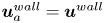 $\boldsymbol {u}_a^{wall}=\boldsymbol {u}^{wall}$. Zero flux of species at the wall is implied by the absence of diffusion velocity in the species equilibrium velocity
 $\boldsymbol {u}^{wall}$.
Finally, we comment that the change of composition due to chemical reaction is due entirely to the reaction term (2.32) in the collision step (2.24). The collision is executed on all the fluid nodes, including the wall interface nodes. Therefore, the change of composition at the wall due to chemical reactions is handled automatically in the collision. In this work, we restrict ourselves to chemically inert walls by using the same reaction mechanism at the wall interface nodes as that at the fluid nodes. However, this approach can also be used for the situations involving catalytic reactions; see e.g. Falcucci et al. (Reference Falcucci2016, Reference Falcucci, Amati, Krastev, Montessori, Yablonsky and Succi2017). In order to implement a catalytic wall reaction, the reaction mechanism at the interface nodes needs to be replaced by a catalytic reaction mechanism, while the TMS procedure described in this section remains unchanged.
4.3. Inlet
The flux boundary condition is used widely to model the inlet in multicomponent flows (Kee et al. Reference Kee, Coltrin and Glarborg2003; Pizza et al. Reference Pizza, Frouzakis, Mantzaras, Tomboulides and Boulouchos2008a, Reference Pizza, Frouzakis, Mantzaras, Tomboulides and Boulouchos2010; Goodwin et al. Reference Goodwin, Speth, Moffat and Weber2018). The rationale of this boundary condition is that it prescribes only the incoming mass fluxes of species  $\rho _a^{in}\boldsymbol {u}^{in}$. Because only the incoming mass flux is prescribed and not the mass itself, the composition at the inlet interface node is not fixed to the incoming composition
 $Y^{in}$. This degree of freedom is necessary as light species such as hydrogen have the capability to diffuse fast enough and thus are able to propagate upstream into the inlet. Therefore, the composition at the inlet interface node is not a fixed set of parameters but is rather a result of a balance between the mass flux inside the domain and the inlet mass flux. Below, we establish the flux boundary condition for the multicomponent lattice Boltzmann setting.
In figure 3, the inlet boundary is represented by a dotted vertical blue line. The inlet boundary condition is applied on the interface nodes where incoming discrete velocities  $\boldsymbol {c}_i$,
 $i\in \mathcal {D}$, are represented by dotted blue arrows. With the inlet data for mass flux
 $\rho ^{in} \boldsymbol {u}^{in}$, composition
 ${Y}^{in}$ and temperature
 $T^{in}$, populations at the interface node are derived in the following steps.
(i) The inlet density
$\rho ^{in}$ and composition ${Y}^{in}$, together with the inlet velocity $\boldsymbol {u}^{in}$ and temperature $T^{in}$, specify uniquely the inlet equilibrium populations $f_i^{in}$, $g_i^{in}$ and $f_{ai}^{in}$ at the inlet interface node:
(4.15)\begin{gather} \{f_i^{in},g_i^{in}\}=\{f_i^{eq},g_i^{eq}\}(\rho^{in}, Y^{in},\boldsymbol{u}^{in},T^{in}), \end{gather}(4.16)\begin{gather}f_{ai}^{in}=f_{ai}^{eq}(\rho^{in}Y_a^{in}, \boldsymbol{u}^{in},T^{in}). \end{gather}(ii) With the incoming populations set to the inlet equilibrium and the outgoing populations known, we find the local density
$\rho ^{loc}$, flow velocity $\boldsymbol {u}^{loc}$, composition ${Y}^{loc}$ and temperature $T^{loc}$ at the interface node (see § A.2 of Appendix A). With the local parameters, the following equilibrium populations are uniquely specified on the momentum, energy and species lattices:
(4.17)\begin{gather} \{f_i^{loc},g_i^{loc}\}= \{f_i^{eq},g_i^{eq}\}(\rho^{loc},Y^{loc},\boldsymbol{u}^{loc},T^{loc}), \end{gather}(4.18)\begin{gather}f_{ai}^{loc}= f_{ai}^{eq}(\rho^{loc}Y_a^{loc},\boldsymbol{u}^{loc},T^{loc}). \end{gather}(iii) Replacing the local flow velocity
$\boldsymbol {u}^{loc}$ and temperature $T^{loc}$ with the target values $\boldsymbol {u}^{in}$ and $T^{in}$, the following target equilibrium populations are identified:
(4.19)\begin{gather} \{f_i^{tgt},g_i^{tgt}\} = \{f_i^{eq},g_i^{eq}\}(\rho^{loc},Y^{loc},\boldsymbol{u}^{in},T^{in}), \end{gather}(4.20)\begin{gather}f_{ai}^{tgt}= f_{ai}^{eq}(\rho^{loc}Y_a^{loc},\boldsymbol{u}^{in},T^{in}). \end{gather}(iv) Finally, all populations at the inlet interface nodes are updated as follows:
(4.21)\begin{gather} \{f^{inlet}_i,g^{inlet}_i\} = \left\{ \begin{array}{@{}ll} \{f_i^{tgt} + f_i^{in} - f_i^{loc},g_i^{tgt} + g_i^{in} - g_i^{loc}\}, & \text{if } i \in \mathcal{D}, \\[3pt] \{f_i^{tgt}+f_i - f_i^{loc},g_i^{tgt} + g_i - g_i^{loc}\}, & \text{otherwise}, \\ \end{array}\right. \end{gather}(4.22)\begin{gather}{f^{inlet}_{ai}} = \left\{ \begin{array}{@{}ll} f_{ai}^{tgt} + f_{ai}^{in} - f_{ai}^{loc}, & \text{if } i \in \mathcal{D},\\[3pt] f_{ai}^{tgt}+f_{ai} - f_{ai}^{loc}, & \text{otherwise }. \\ \end{array}\right. \end{gather}


It is straightforward to verify that the populations (4.21) and (4.22) at step (iv) imply the target values  $\boldsymbol {u}^{in}$ and
 $T^{in}$ for the velocity and temperature at the interface node, respectively. At the same time, the composition and density at the interface node are identified as
 ${Y}^{loc}$ and
 $\rho ^{loc}$, respectively. The latter are derived in step (ii) by taking into account the outgoing populations, and are different, in general, from the inlet values
 ${Y}^{in}$ and
 $\rho ^{in}$. Thus the outgoing populations contribute to the balance between the incoming and outgoing mass fluxes as required by the flux boundary condition. It is instructive to compare with the TMS wall boundary condition of § 4.2.2 where the local composition at the interface node was determined by the bounce-back step, (4.7) and (4.8). In the present case, at step (ii), the local composition is computed using the equilibrium at the inflow properties for the incoming populations. Note that while the inlet composition
 $Y^{loc}$ is already determined at step (ii), the purpose of the remaining steps is to enforce the inlet velocity
 $\boldsymbol {u}^{in}$ and temperature
 $T^{in}$. Hence whenever the inlet temperature and velocity need not be strictly imposed, it is sufficient to terminate the algorithm at step (ii) and to apply the local equilibria (4.17) and (4.18). With this simplification, the velocity and temperature acquire local values
 $\boldsymbol {u}^{loc}$ and
 $T^{loc}$, respectively, rather than the target values
 $\boldsymbol {u}^{in}$ and
 $T^{in}$. The latter simplification was validated in Sawant et al. (Reference Sawant, Dorschner and Karlin2021a) with the simulation of diffusion in opposed jets. The mass fractions at the inlets of both jets matched the reference solution by Cantera, which employs a macroscopic realization of the flux boundary condition. While the simplified inlet realization (4.17) and (4.18) can be regarded as a good approximation to the macroscopic flux boundary condition, in this work we rather use the inlet populations (4.21) and (4.22) to ensure that the inlet velocity and temperature are imposed exactly.
4.4. Outlet
Unlike the inlet and the wall, the values of the macroscopic state variables are usually unknown at the outlet. To that end, we apply the local one-dimensional inviscid (LODI) approximation by Poinsot & Lele (Reference Poinsot and Lele1992). The LODI approximation is based on the characteristics of compressible Euler equations, i.e. (3.29), (3.30) and (3.31) without dissipation terms. The LODI boundary condition allows both the pressure fluctuations travelling as sound waves as well as the convection disturbances travelling as entropy waves to exit the computational domain with minimum reflection (Poinsot & Lele Reference Poinsot and Lele1992). The LODI approximation is derived for a single-component fluid and therefore predicts the outlet density  $\rho ^{out}$, velocity
 $\boldsymbol u^{out}$ and temperature
 $T^{out}$, which can be used directly in the present mean-field formulation of the mixture. In addition, we need also to specify the composition
 ${Y}^{out}$ at the outlet. Consistent with the LODI approximation, we use the advection part of the species equation (2.22), which is discretized at the outlet interface node with forward Euler scheme to give
 \begin{equation} Y_a^{out}(\boldsymbol{x},t) = Y_a^{out}(\boldsymbol{x},t- \delta t) -\delta t\,\boldsymbol{u}^{out}(\boldsymbol{x},t- \delta t) \boldsymbol{\cdot}\boldsymbol{\nabla} Y_a^{out}(\boldsymbol x,t- \delta t),\end{equation}
where mass fraction  $Y_a^{out}(\boldsymbol {x},t- \delta t)$ is known from the previous time step, while
 $\boldsymbol {u}^{out}$ is the LODI outlet velocity. The gradient
 $\boldsymbol {\nabla } Y_a^{out}$ is evaluated by backward finite difference. Armed with the outlet data, we proceed to specify the populations at the outlet interface node, following essentially the steps already familiar from the wall and inlet construction.
(i) Outlet data
$Y_a^{out}$, $\rho ^{out},\boldsymbol {u}^{out}$ and $T^{out}$ specify uniquely the equilibrium populations $f_i^{out}$, $g_i^{out}$ and $f_{ai}^{out}$ at the outlet interface node:
(4.24)\begin{gather} \{f_i^{out},g_i^{out}\}= \{f_i^{eq},g_i^{eq}\}(\rho^{out},Y^{out}, \boldsymbol{u}^{out},T^{out}), \end{gather}(4.25)\begin{gather}f_{ai}^{out}= f_{ai}^{eq}(\rho^{out} Y_a^{out}, \boldsymbol{u}^{out},T^{out}). \end{gather}(ii) With the incoming populations set to the outlet equilibrium, we find the local density
$\rho ^{loc}$, flow velocity $\boldsymbol {u}^{loc}$, mass fractions ${Y}^{loc}$ and temperature $T^{loc}$ at the outlet interface node (see § A.3 of Appendix A). Based on these local parameters, the local equilibrium populations are specified uniquely on the momentum, energy and species lattices:
(4.26)\begin{gather} \{f_i^{loc},g_i^{loc}\}=\{f_i^{eq},g_i^{eq}\}(\rho^{loc}, Y^{loc},\boldsymbol{u}^{loc},T^{loc}), \end{gather}(4.27)\begin{gather}f_{ai}^{loc}=f_{ai}^{eq}(\rho^{loc}Y_a^{loc}, \boldsymbol{u}^{loc},T^{loc}). \end{gather}(iii) Finally, all populations of the momentum, energy and species lattices at the outlet interface node are updated as
(4.28)\begin{gather} \{f^{outlet}_i,g^{outlet}_i\} = \left\{ \begin{array}{@{}ll} \{2 f_i^{out} - f_i^{loc},2 g_i^{out} - g_i^{loc}\}, & \text{if } i \in \mathcal{D}, \\[3pt] \{f_i^{out}+f_i - f_i^{loc},g_i^{out} + g_i - g_i^{loc}\}, & \text{otherwise}, \\ \end{array} \right. \end{gather}(4.29)\begin{gather}{f^{outlet}_{ai}} = \left\{ \begin{array}{@{}ll} 2 f_{ai}^{out} - f_{ai}^{loc}, & \text{if } i \in \mathcal{D}, \\[3pt] f_{ai}^{out}+f_{ai} - f_{ai}^{loc}, & \text{otherwise}. \\ \end{array}\right. \end{gather}


With populations (4.28) and (4.29) at step (iii), the macroscopic fields at the outlet are set to the target values  $\rho ^{out}$,
 $\boldsymbol {u}^{out}$,
 $T^{out}$ and
 $Y^{out}$, as prescribed by the LODI approximation and (4.23). Although the same is achieved by the equilibrium populations at step (i), the non-equilibrium part of the incoming populations is taken into consideration and modelled with the local state in step (ii). Thus the present construction of the outlet is similar to the TMS wall boundary condition of § 4.2.2.
5. Wall-bounded reactive flow
In order to test the proposed boundary conditions, we perform the computation of combustion in microtubes. The results are validated with the DNS of Pizza et al. (Reference Pizza, Frouzakis, Mantzaras, Tomboulides and Boulouchos2008b) for two-dimensional (2-D) microchannels and Pizza et al. (Reference Pizza, Frouzakis, Mantzaras, Tomboulides and Boulouchos2010) for a 3-D microtube. The set-up involves combustion of a premixed hydrogen/air mixture in a tube over a range of inlet velocities  $u_{in}$ of the unburnt mixture. The fuel-lean unburnt mixture of equivalence ratio
 $\phi =0.5$ at temperature
 $T_u=300$ K and pressure
 $1 \ \text {atm}$ enters a microchannel with
 $l/d=10$. Here,
 $l$ is the length of the tube, and
 $d$ is its diameter. The mixture gets ignited due to hot isothermal walls that are maintained at temperature
 $T_w=960\ \text {K}$. The wall temperature is increased from
 $300\ \text {K}$ at the inlet to
 $960 \text {K}$ using a hyperbolic tangent profile at a distance of about
 $l/20$ from the inlet. For this premixed initial condition, the burning velocity is obtained as
 $S_L=59\ \text {cm}\ \text {s}^{-1}$, and the flame thickness is obtained as
 $\delta _{f}=0.043\ \text {cm}$ from solving a 1-D flame propagation set-up with the LBM in § 3.8.
5.1. Premixed hydrogen/air flames in a microchannel
For the 2-D simulations, we choose channel diameter  $d=1\ \text {mm}$, which corresponds to width
 $2.3256\,\delta _{f}$ in terms of flame thickness. The spatial resolution corresponds to approximately
 $15$ nodes per flame thickness. As studied in Pizza et al. (Reference Pizza, Frouzakis, Mantzaras, Tomboulides and Boulouchos2008b) for the same channel width, the flame exhibits different dynamics depending on the inlet velocity. At low inlet velocity of about
 $u_{in}=10 \ \text {cm}\ \text {s}^{-1}$, periodic ignition and extinction of the flame are observed. The inlet velocity is then increased progressively until the oscillatory behaviour ceases and a stable flame can be sustained near the inlet of the channel. A further increase of the inlet velocity to
 $u_{in}=75\ \text {cm}\ \text {s}^{-1}$ results in a symmetric ‘V-shaped flame’ in the channel, the flame being concave towards the unburnt mixture. Finally, at inflow higher than
 $u_{in}=165\ \text {cm}\ \text {s}^{-1}$, stable asymmetric flames are formed that shift downstream with increasing inlet velocity. The Reynolds number corresponding to the inlet velocity varies between
 ${Re}=5.36$ and
 ${Re}=88.52$, the reference length being the channel width, and the reference viscosity corresponding to the viscosity at inlet composition and temperature.
5.1.1. Periodic ignition and extinction
The fluid in the bulk of the domain is initialized with the inlet unburnt composition, and the inlet velocity is set to  $u_{in}=10\ \text {cm} \text {s}^{-1}$. The initial temperature of the fluid in the bulk follows the wall temperature profile. As the fresh mixture passes between the heated walls, the reactants break into radicals that build up in the channel over time. This build up of radicals is associated with a long period of inactivity after which the mixture achieves a radical runaway and eventually a thermal runaway, leading to ignition. The mixture ignites at some distance downstream, as seen in figure 4, which shows the hydroxide mass fraction that we will use as a marker to represent the ‘flame’ itself. The flame first forms a concentrated nearly circular structure that then propagates in both upstream and downstream directions, as is visible in figure 4. This flame splitting occurs as the flame consumes the relatively fresh mixture in both possible directions. The panels in figure 5 show the mass fraction of hydrogen that is the deficient reactant. The flame then propagates and splits, consuming the deficient reactant in its path. The part of the flame travelling upstream is extinguished at the cold inlet, whereas the part travelling downstream exits the channel through the outlet. Subsequently, the channel is again filled with the fresh mixture from the inlet, and the process repeats periodically. In this regime, the maxima of all the species mass fractions as well as that of the temperature are located on the centreline of the channel. This behaviour is consistent with the DNS of Pizza et al. (Reference Pizza, Frouzakis, Mantzaras, Tomboulides and Boulouchos2008b) and the subsequent simulations of Alipoor & Mazaheri (Reference Alipoor and Mazaheri2016). This phenomenon, which is also referred to as a flame with repetitive extinction and ignition (FREI), has also been observed in methane/air combustion experiments of Maruta et al. (Reference Maruta, Kataoka, Kim, Minaev and Fursenko2005) and numerical simulations of Norton & Vlachos (Reference Norton and Vlachos2003). The periodicity of the ignition–extinction behaviour has been presented through the variation of the integrated heat release rate with time in figure 6. In that figure, the heat release rate has been normalized with respect to the heat release rate of the unburnt state. The ignition events are seen to produce a rise in the integrated heat release rate by
 $8$ orders of magnitude. The peaks are localized in time with average frequency approximately
 $111 \ \text {Hz}$. This is in good agreement with the frequency
 $106.9 \ \text {Hz}$ reported in Pizza et al. (Reference Pizza, Frouzakis, Mantzaras, Tomboulides and Boulouchos2008b). Table 1 shows the convergence of the ignition–extinction frequency with resolution. Between the two largest resolutions, the frequency changed by only
 $2.7\,\%$ with an increase in the spatial resolution by
 $50\,\%$. Therefore, the computations are considered to be converged with respect to the resolution. The maximum velocity of the upstream propagation of the flame is found to be
 $16.8 \text {cm}\ \text {s}^{-1}$, and that of the downstream propagation is found to be
 $20\ \text {cm}\ \text {s}^{-1}$ from the LBM simulations. For comparison, the maximum upstream propagation speed is reported to be
 $15\ \text {cm}\ \text {s}^{-1}$ in Pizza et al. (Reference Pizza, Frouzakis, Mantzaras, Tomboulides and Boulouchos2008b). Overall, the LBM results agree well quantitatively with the DNS results.
Contours of the mass fraction of hydroxide OH showing ignition, flame formation, splitting and propagation of the flame. Unburnt mixture enters the domain through the inlet on the left. Times are (a)  $t= 0.045741$ s, (b)
 $t=0.045767$ s, (c)
 $t=0.045819$ s, and (d)
 $t=0.045897$ s.

Contours of the mass fraction of hydrogen H $_2$ showing its consumption during the ignition–extinction process at time instants marked in the inset in figure 6. Unburnt mixture enters the domain through the inlet on the left. Times are (a)
 $t= 0.045741$ s, (b)
 $t=0.045767$ s, (c)
 $t=0.045819$ s, and (d)
 $t=0.045897$ s.

Integrated heat release rate versus time in the periodic ignition–extinction regime. The frequency from the LBM simulation is approximately  $111\ \text {Hz}$; the reference frequency from the DNS of Pizza et al. (Reference Pizza, Frouzakis, Mantzaras, Tomboulides and Boulouchos2008b) is
 $106.9$ Hz. Time instants corresponding to figure 4 are marked by red crosses in the inset.

Frequencies of the ignition–extinction phenomenon obtained from LBM simulations run with different spatial resolutions.

5.1.2. V-shaped stable flames
Using the solution from the ignition–extinction regime as an initial condition, the inlet velocity is increased progressively to  $u_{in}=75 \text {cm}\ \text {s}^{-1}$. In this regime, there is a sufficient flow of fresh mixture to sustain combustion and therefore a stable flame is formed in the channel. As is evident in figure 7, the flame assumes a ‘V-shaped’ structure that is concave towards the unburnt mixture. At this inlet velocity, the structure of all the species is symmetric about the centreline. The maxima of the mass fractions of all the species are located on the centreline, except for the hydrogen radical. The hydrogen radical has a high molecular diffusivity, causing it to shift away from the channel centreline. This is evident from the line contours in figure 8. The heat release rate contours in figure 9 show a localized heat release at the upstream interface of the flame. Also, the heat release rate contour follows a concave curvature that is similar to mass fraction contours of the hydroxide and the hydrogen radical. A maximum temperature
 $1715\ \text {K}$ is attained in the flame. Shifting of the maxima of hydrogen at this inflow velocity as well as the concave shape of the flame is consistent with the findings of Pizza et al. (Reference Pizza, Frouzakis, Mantzaras, Tomboulides and Boulouchos2008b). With an increasing inlet velocity, the flame stabilizes further downstream from the inlet due to a relative increase in the difference between the velocity of the fresh mixture and the flame speed. Furthermore, at higher inlet velocities, more species shift away from the tube centreline. In a 3-D microtube, the shifting of the maxima causes the flame to form a ring-like structure (Pizza et al. Reference Pizza, Frouzakis, Mantzaras, Tomboulides and Boulouchos2010) around the tube centreline. We explore this phenomenon in detail in the corresponding 3-D simulations.
V-shaped flames: contours of hydroxide OH mass fraction. The flame is concave towards the unburnt mixture coming in from the left.

V-shaped flames: contours of hydrogen radical H mass fraction. Line contours highlight the shift of maxima away from the centreline.

V-shaped flames: contours of the heat release rate (HRR) normalized by the heat release rate of the unburnt mixture.

5.1.3. Asymmetric stable flames
Starting from the V-shaped flame as an initial condition, we increase the inlet flow velocity gradually to  $u_{in}=300\ \text {cm}\ \text {s}^{-1}$. After shifting downstream and maintaining its symmetric shape for some time, the flame transitions into an asymmetric stable flame. At the upstream interface between the flame and the unburnt mixture, a flame forming an acute angle with the lower wall is termed a lower asymmetric flame (Pizza et al. Reference Pizza, Frouzakis, Mantzaras, Tomboulides and Boulouchos2008b). Similarly, a flame forming an acute angle with the upper wall is termed an upper asymmetric flame. As shown in figure 10, a lower symmetric flame was first encountered in our computation. Interestingly, the asymmetric flame is metastable in this regime. The flame can be made to transition from a lower asymmetric shape to an upper asymmetric shape by heating the lower wall momentarily and then restoring the wall temperature back to the previous wall temperature
 $960\ \text {K}$. A snapshot of the flame during this transition is shown in figure 11. An upper asymmetric flame formed as a result of the temperature perturbation is shown in figure 12. The resultant flame is also metastable and remains in its upper asymmetric shape unless perturbed. The heat release rate profile is very similar to the profile of the mass fraction of hydrogen, except for the location of the maxima. The maxima of the heat release rate occur at the walls in this regime. The distance of the flame from the inlet remains unchanged. In the LBM simulations, the location of the beginning of the flame is
 $0.24l$ from the inlet, which is in good agreement with
 $0.21l$ obtained by the DNS of Pizza et al. (Reference Pizza, Frouzakis, Mantzaras, Tomboulides and Boulouchos2008b). The asymmetric nature of the flame and its metastable behaviour are consistent with the findings of Pizza et al. (Reference Pizza, Frouzakis, Mantzaras, Tomboulides and Boulouchos2008b) for this regime.
Lower asymmetric flame in the microchannel: contours of hydroxide OH mass fraction (a), hydrogen radical H mass fraction (b) and heat release rate (c).

Flame transitioning from a lower asymmetric shape to an upper asymmetric flame: contours of hydroxide mass fraction (a), hydrogen mass fraction (b) and heat release rate (c).

Upper asymmetric flame in the microchannel: contours of hydroxide mass fraction (a), hydrogen mass fraction (b) and heat release rate (c).

5.2. Premixed hydrogen/air flame in microtube
For 3-D simulations, we choose the circular tube set-up with width  $d=1.5\ \text {mm}$ from the simulations in Pizza et al. (Reference Pizza, Frouzakis, Mantzaras, Tomboulides and Boulouchos2010). Richer dynamics is exhibited by this wide tube as compared to the narrower
 $1 \,\text {mm}$ tube. The composition of the incoming mixture is the same as for the 2-D simulations. The aspect ratio is also unchanged at
 $l/d=10$. The diameter corresponds to flame thickness
 $d=3.4884\,\delta _f$. With the viscosity of the mixture at the inlet unburnt composition and at the inlet temperature as reference, the inlet velocity as the reference velocity and the diameter of the tube as the length scale, the Reynolds number is
 ${Re}=80.47$. We use a computational domain of
 $l \times d \times d=540 \times 54 \times 54$ nodes, which translates into a spatial resolution of
 $15.5$ computational nodes per flame thickness. As discussed in § 5.1 with the aid of table 1, this resolution was sufficient to produce correct and converged results in the 2-D ignition–extinction simulations. In the 3-D simulations, we explore the ‘open axisymmetric flame’ characterized by the maximum of the hydroxide radical being shifted away from the tube centreline. The isosurfaces of hydroxide therefore form a ring-shaped structure around the tube centreline. In the DNS of Pizza et al. (Reference Pizza, Frouzakis, Mantzaras, Tomboulides and Boulouchos2010), such open flames are observed for an inflow velocity over two disconnected ranges,
 $60\ \text {cm}\ \text {s}^{-1} \leq u_{in} \leq 100\ \text {cm} \text {s}^{-1}$ and
 $170\ \text {cm}\ \text {s}^{-1} \leq u_{in} \leq 350\ \text {cm}\ \text {s}^{-1}$. In this work, we verify the existence of open flames by performing a simulation at an inflow of
 $u_{in}=100\ \text {cm}\ \text {s}^{-1}$. The inlet velocity is increased gradually to
 $u_{in}=200\ \text {cm}\ \text {s}^{-1}$ and then to
 $u_{in}=300\ \text {cm}\ \text {s}^{-1}$. We measure the positions of the flame at these three inlet conditions and compare with the flame positions reported for axisymmetric simulations in Pizza et al. (Reference Pizza, Frouzakis, Mantzaras, Tomboulides and Boulouchos2010).
The bulk of the fluid in the tube is initialized with the inflow velocity  $u_{in}=100\ \text {cm}\ \text {s}^{-1}$, and the temperature is initialized to the wall temperature profile. The composition is initialized with a 1-D laminar flame solution computed for the same equivalence ratio as this 3-D set-up. The initial pressure in the domain is homogeneous at
 $1 \text {atm}$. As a consequence of the initial conditions and the inflow velocity, the ignition–extinction regime is not encountered. The incoming fresh mixture enters the tube at a speed that is nearly twice the flame speed. Therefore, the resulting flame does not propagate upstream into the inlet and stabilizes at a distance downstream of the inlet. The flame has the location of the maximum of the hydroxide radical and the temperature shifted away from the longitudinal axis of the tube. Therefore, as is visible in figure 13, isosurfaces of the mass fraction of hydroxide form ring-shaped structures. This type of ring-like flame is called an ‘open flame’ in Pizza et al. (Reference Pizza, Frouzakis, Mantzaras, Tomboulides and Boulouchos2010). At
 $u_{in}=100\ \text {cm}\ \text {s}^{-1}$, the open flame is axisymmetric and maintains a fixed distance of approximately
 $0.1 l$ from the inlet. The maximum temperature in the flame is
 $1649$ K. Figure 14 shows isosurfaces of the mass fraction of the hydrogen radical, which also forms a ring structure similar to the hydroxide radical. Streamlines of the fluid velocity in figure 14 show a marked acceleration in the fluid velocity downstream of the flame location. The post-combustion fluid in the tube is seen to have attained a maximum velocity that is
 $9.3$ times that of the inlet velocity. The maxima of the fluid velocity reside on the tube centerline. In figure 15, we compare the flame position at different inlet velocities as obtained from our 3-D simulations with the flame positions provided from the 2-D axisymmetric simulations by Pizza et al. (Reference Pizza, Frouzakis, Mantzaras, Tomboulides and Boulouchos2010). The flame position is defined by the streamwise location of maximum temperature, measured downstream from the inlet. Good agreement is obtained with the axisymmetric DNS simulations. A new oscillatory mode causing the flame to pulsate in the streamwise direction was observed in the axisymmetric simulations but not in the 3-D simulations by Pizza et al. (Reference Pizza, Frouzakis, Mantzaras, Tomboulides and Boulouchos2010). We performed 3-D simulations in this work and did not observe the pulsating mode, which confirms their observation.
Open flame in the microchannel: isosurfaces of  $Y_{\rm OH}$ and slice of temperature contour at a
 $Z$ plane passing through the centre.

Open flame in the microchannel: isosurfaces of  $Y_{\rm H}$ and streamlines of the fluid velocity.

Position of the flame measured downstream from the inlet versus the fluid velocity imposed at the inlet. The position is normalized by the diameter  $d$ of the tube. The black circles belong to 2-D axisymmetric simulations of Pizza et al. (Reference Pizza, Frouzakis, Mantzaras, Tomboulides and Boulouchos2010), and the red squares belong to 3-D LBM simulations.

For these 3-D simulations, the required mesh size and computational costs are similar to the fourth-order spectral element code of Pizza et al. (Reference Pizza, Frouzakis, Mantzaras, Tomboulides and Boulouchos2008a,Reference Pizza, Frouzakis, Mantzaras, Tomboulides and Boulouchosb, Reference Pizza, Frouzakis, Mantzaras, Tomboulides and Boulouchos2010). In particular, for the same level of accuracy (see table 1), our simulations required approximately  $8\,\%$ more grid points and cost
 $15\,\%$ less node hours (measured on a CRAY XC40 system with 2x Intel Xeon E5-2695 v4 at 2.10 GHz per node) compared to what is reported in Pizza et al. (Reference Pizza, Frouzakis, Mantzaras, Tomboulides and Boulouchos2010). Our profiling also indicates that for simulations with detailed chemistry, the performance is limited by the chemical kinetics solver rather than the hydrodynamics solver. In our simulations, approximately
 $71\,\%$ of the total computing time is spent in the chemical kinetics solver, which explains the similar computational costs overall.
6. Conclusion
In this paper, we aimed to develop an accurate and robust lattice Boltzmann model for reactive flows of practical interest. In Sawant et al. (Reference Sawant, Dorschner and Karlin2021a), we proposed a lattice Boltzmann framework consisting of  $M+2$ lattice Boltzmann equations for multicomponent mixtures of ideal gases. We introduced a new LBM system for the Stefan–Maxwell diffusion along with a reduced, mean-field description of the mixture momentum and energy using a two-population approach. Thermodynamic consistency of this model allowed us to account naturally for the temperature and energy changes due to chemical reactions by including the energy of formation, which avoids any ad hoc modelling for the heat of reaction. The proposed model uses the extended LBM of Saadat et al. (Reference Saadat, Dorschner and Karlin2021a) for the mean fields and a multistep approach for integrating the mass source terms. Furthermore, we introduced novel kinetic boundary conditions for walls, inlets and outlets that are compatible with the underlying reactive flow model.
Our model was validated in detail, starting from a zero-dimensional perfectly stirred reactor and the one-dimensional laminar flame. The accuracy of the boundary conditions was assessed by simulations of premixed hydrogen/air flames in a microtube in both two and three dimensions. In all cases, the results were found to be in excellent agreement with reference and DNS solutions that can be found in the literature.
To conclude, the proposed model is not only a viable alternative to traditional reactive computational fluid dynamics but also the first model that is capable of solving reactive flows entirely in the lattice Boltzmann framework. Thus our model inherits well-known merits of the LBM, such as excellent parallel efficiency and accuracy (exact advection), which has been shown to be advantageous compared to conventional (high-order) approaches (see e.g. Marié, Ricot & Sagaut Reference Marié, Ricot and Sagaut2009; Mulloth et al. Reference Mulloth, Sawant, Haider, Sharma and Sengupta2015; Dorschner et al. Reference Dorschner, Chikatamarla and Karlin2016). While our model can be used seamlessly for low and moderately high Mach number flows (Saadat et al. Reference Saadat, Dorschner and Karlin2021a,Reference Saadat, Hosseini, Dorschner and Karlinb), different kinetic flow models, such as the particle-on-demand method (Dorschner et al. Reference Dorschner, Bösch and Karlin2018; Reyhanian, Dorschner & Karlin Reference Reyhanian, Dorschner and Karlin2020; Kallikounis, Dorschner & Karlin Reference Kallikounis, Dorschner and Karlin2021), can be used to further extend the model to supersonic and hypersonic regimes. Finally, accurate diffusion models such as the Stefan–Maxwell diffusion are most naturally implemented in a kinetic framework owing to their origin in kinetic theory, and become particularly important for light species that can, for instance, be found in fuel cells (Hsing & Futerko Reference Hsing and Futerko2000; Stockie, Promislow & Wetton Reference Stockie, Promislow and Wetton2003; Suwanwarangkul et al. Reference Suwanwarangkul, Croiset, Fowler, Douglas, Entchev and Douglas2003; Lindstrom & Wetton Reference Lindstrom and Wetton2017), which opens interesting opportunities for optimizing clean energy applications.
Funding
This work was supported by European Research Council (ERC) Advanced Grant no. 834763-PonD. Computational resources at the Swiss National Super Computing Center CSCS were provided under grant no. s1066.
Declaration of interests
The authors report no conflict of interest.
Appendix A. Boundary conditions: local moments
A.1. Tamm–Mott-Smith wall boundary condition
After the incoming populations are set to the target equilibrium, we find the local density  $\rho ^{loc}$, flow velocity
 $\boldsymbol {u}^{loc}$, mass fractions
 ${Y}^{loc}$, species velocities
 $\boldsymbol {u}_a^{loc}$ and temperature
 $T^{loc}$ at the interface node as
 \begin{gather} \sum_{i\in\mathcal{D}} f_i^{tgt} +\sum_{i\notin\mathcal{D}} f_i = \rho^{loc}, \end{gather}
 \begin{gather}\sum_{i\in\mathcal{D}} \boldsymbol{c}_if_i^{tgt} +\sum_{i\notin\mathcal{D}} \boldsymbol{c}_if_i = \rho^{loc} \boldsymbol{u}^{loc}, \end{gather}
 \begin{gather}{\sum_{i\in \mathcal{D}}f_{ai}^{tgt}+\sum_{i\notin \mathcal{D}}f_{ai}=\rho^{loc}{Y}_a^{loc},\quad a=1,\ldots,M}, \end{gather}
 \begin{gather}{\sum_{i\in \mathcal{D}} \boldsymbol{c}_i f_{ai}^{tgt}+\sum_{i\notin \mathcal{D}} \boldsymbol{c}_i f_{ai}=\rho_a^{loc}\boldsymbol{u}_a^{loc},\quad a=1,\ldots,M}, \end{gather}
 \begin{gather}\sum_{i\in\mathcal{D}} g_i^{tgt} +\sum_{i\notin\mathcal{D}} g_i = \rho^{loc}\sum_{a=1}^M{Y^{loc}_a}\left[U_a^0 + \int_{T_0}^{T^{loc}} {C}_{a,v}(T')\, {\rm d} T'\right]+\frac{1}{2}\rho^{loc}(u^{loc})^2. \end{gather}
A.2. Inlet
After the incoming populations are set to the inlet equilibrium and the outgoing populations are known, we find the local density  $\rho ^{loc}$, flow velocity
 $\boldsymbol {u}^{loc}$, composition
 ${Y}^{loc}$ and temperature
 $T^{loc}$ at the interface node as
 \begin{gather} \sum_{i\in\mathcal{D}} f_i^{in} +\sum_{i\notin\mathcal{D}} f_i = \rho^{loc}, \end{gather}
 \begin{gather}\sum_{i\in\mathcal{D}} \boldsymbol{c}_if_i^{in} +\sum_{i\notin\mathcal{D}} \boldsymbol{c}_if_i = \rho^{loc} \boldsymbol{u}^{loc}, \end{gather}
 \begin{gather}\sum_{i\in \mathcal{D}}f_{ai}^{in}+\sum_{i\notin \mathcal{D}}f_{ai}=\rho^{loc}{Y}_a^{loc},\quad a=1,\ldots,M, \end{gather}
 \begin{gather}\sum_{i\in\mathcal{D}} g_i^{in} +\sum_{i\notin\mathcal{D}} g_i = \rho^{loc}\sum_{a=1}^M{Y^{loc}_a}\left[U_a^0 + \int_{T_0}^{T^{loc}} {C}_{a,v}(T')\, {\rm d} T'\right]+\frac{1}{2}\rho^{loc}(u^{loc})^2. \end{gather}
A.3. Outlet
After the incoming populations are set to the outlet equilibrium, we find the local density  $\rho ^{loc}$, flow velocity
 $\boldsymbol {u}^{loc}$, mass fractions
 ${Y}^{loc}$, and temperature
 $T^{loc}$ at the outlet interface node as
 \begin{gather} \sum_{i\in\mathcal{D}} f_i^{out} +\sum_{i\notin\mathcal{D}} f_i = \rho^{loc}, \end{gather}
 \begin{gather}\sum_{i\in\mathcal{D}} \boldsymbol{c}_i f_i^{out} +\sum_{i\notin\mathcal{D}} \boldsymbol{c}_if_i = \rho^{loc} \boldsymbol{u}^{loc}, \end{gather}
 \begin{gather}{\sum_{i\in \mathcal{D}}f_{ai}^{out}+\sum_{i\notin \mathcal{D}}f_{ai}=\rho^{loc}{Y}_a^{loc},\quad a=1,\ldots,M}, \end{gather}
 \begin{gather}\sum_{i\in\mathcal{D}} g_i^{out} +\sum_{i\notin\mathcal{D}} g_i = \rho^{loc}\sum_{a=1}^M{Y^{loc}_a}\left[U_a^0 + \int_{T_0}^{T^{loc}} {C}_{a,v}(T')\, {\rm d} T'\right]+\frac{1}{2}\rho^{loc}(u^{loc})^2. \end{gather}
In the preceding text, (A5), (A9) and (A13) are integral equations to be resolved for the temperature  $T^{loc}$; cf. § 3.1 and (3.9).


 Open access

