The model and simulation results

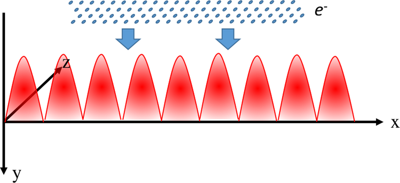
Two-dimensional (2D) PIC simulations were performed using the EPOCH code (Ridgers et al., Reference Ridgers, Kirk, Duclous, Blackburn, Brady, Bennett, Arber and Bell2014; Arber et al., Reference Arber, Bennett, Brady, Lawrence-Douglas, Ramsay, Sircombe, Gillies, Evans, Schmitz and Bell2015). Figure 1 shows the configuration of the electron beam being launched into the linear polarized LSWF. We assume that the LSWF is generated by two Gaussian linearly polarized laser pulses with the same parameters focused in the y–z plane. They counter-propagate along the x axis launched from the left and right boundaries, respectively, and everything is assumed to be constant in the z-direction for the 2D simulations. The vector potential of the counter-propagating lasers is expressed as ${\bi a} = a\cos (kx + {{\rm \omega}} t){\hat{\bf e}}_y + a\cos (kx-{{\rm \omega}} t){\hat{\bf e}}_y$, where $a = a_0\exp [-(y^2 + z^2)/w_0^2 ]$, w ₀ is the laser beam waist radius, a ₀ is the vector potential peak amplitude of one laser normalized by mωc/e, m and e are the electron's mass and charge, respectively, ω is the frequency of laser, and c is the speed of light in vacuum. The laser wavelength is 800 nm and the duration of the LSWF is 100 fs to allow electrons pass through. Then the electric field and magnetic field of the LSWF are expressed as follows:

(1)$$\eqalign{& {\bf E(}{\bi x}{\bf,} {\bi y}{\bf,} {\bi t}{\bf )} = -\partial _t{\bf a} = 2a\sin ({{\rm \omega}} t)\cos (kx){{\hat{\bf e}}}_y \cr & {\bf B(}{\bi x}{\bf,} {\bi y}{\bf,} {\bi t}{\bf )} = \nabla \times {\bf a} = -2a\cos ({{\rm \omega}} t)\sin (kx){{\hat{\bf e}}}_z.} $$

Fig. 1.

Schematic geometry of an electron beam launched into a linear polarized LSWF.

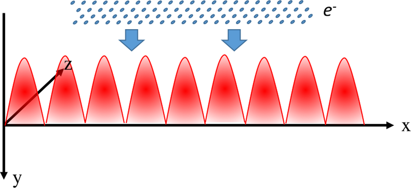
Considering a relativistic electron beam traveling through an LSWF, the electrons with a Gaussian (an uniform) density profile of 6-μm (1-μm) full width in the x (y) direction are launched along the +y axis toward the overlapping lasers, which is parallel to the electric field of the laser field. The motion of the electrons is governed by the Lorentz force equation, $d{\bf P}/dt = -e({\bf E} + {\bf v} \times {\bf B})$. The peak density of the electron beam is set to be 10⁻³n _c (n _c = ε₀m _eω²/e ² the critical density for laser with wavelength of 800 nm), which is far below the critical density to avoid the effect of strong space-charge forces on the LSWF. Since the transverse momentum spread of the electron beam caused by the momentum gain after interaction is about 10% of the initial momentum in our case, the initial energy spread of the electron beam, which is well below 10% from a wakefield accelerator or a linac, has little effect on the density modulation. For simplicity, we represent a planar geometry, i.e., the projection of the momentum of the electron onto the direction of the z axis as equal to zero both before and after scattering.

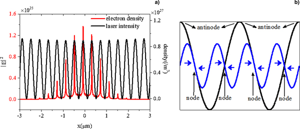
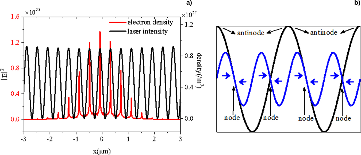
When two counter-propagating traveling lasers form a standing wave, the spatial phase along the propagation direction remains unchanged. Thus, electrons with velocity normal to the direction of laser propagation experience a constant laser phase during the interaction. As Figure 2a shows, the initial electrons of continuous density are modulated into a periodic structure after traversing the LSWF, and the period equals to half the wavelength of the LSWF. Remarkably, each density peak locates at the antinode while each density valley locates at the node of the LSWF. Such discrete electron beam structure is manifested by the special configuration of the LSWF. The electric field value of the LSWF at the nodes remains zero, but the oscillation phases of the amplitude on the two sides of each node are opposite and the electromagnetic field is spatially inhomogeneous. Meanwhile, the electrons traversing across are subjected to the high gradient (i.e., classical ponderomotive force) close to the nodes. The classical ponderomotive force is of the intensity gradient form:

(2)$${\bf F}_{\rm p} = -\displaystyle{{e^2} \over {2{{\rm \varepsilon}} _0mc{{\rm \omega}} ^2}}\nabla \vert {{\bf E}(x)} \vert ^2.$$

Fig. 2.

(a) Electron density integral and laser intensity on the x-axis with electron beam energy γ₀ = 20 and LSWF intensity I = 1 × 10¹⁹ W/cm². (b) Schematic diagram of phase relation of electric field of LSWF (black line) and the ponderomotive force (blue line), the amplitude is adjusted for a better view.

It always propels particles toward areas of low field intensity, thus leading to the scattering of electrons owing to the spatial transverse ponderomotive force. We obtain the components of the ponderomotive force as combining Eqs (1) and (2):

(3)$${\bf F}_{{\rm p}x} = {\rm \Phi} \cdot \exp [-2(y^2 + z^2)/w_0^2 ]\cdot k\cdot \sin (2kx){\hat{\bf e}}_{\bi x},$$

where ${\rm \Phi} = 2e^2a_0^2 /({{\rm \varepsilon}} _0mc{{\rm \omega}} ^2) \times \sin ^2({{\rm \omega}} t)$. According to Eq. (3), the amplitude maximizes at the phase kx = nπ/2 + π/4 (n = 0, 1, 2, …) and turns to be zero at the phase kx = nπ/2, i.e., the nodes and antinodes, as shown in Figure 2b, and the ponderomotive force points to the nodes.

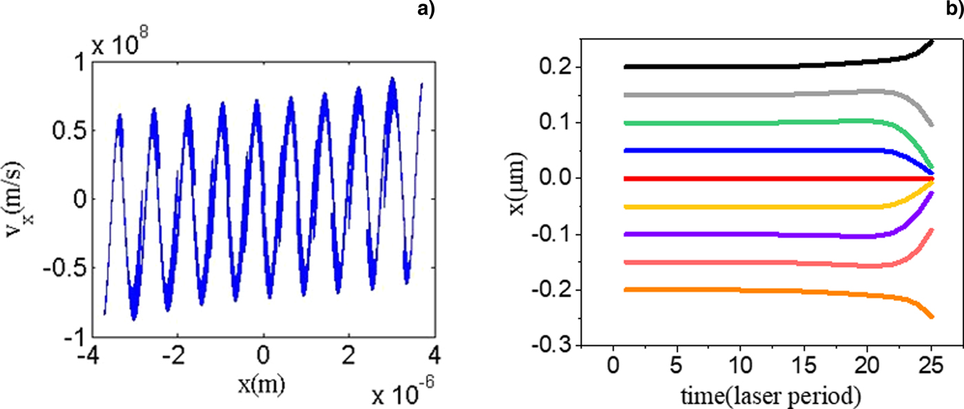
Figure 3a shows the distribution of the electron velocity component along the x direction at the corresponding position in the x axis, when the electrons are inside the standing wave field. The entire distribution goes up from left to right and is antisymmetric owing to the Gaussian envelope of the laser pulse which results in the opposite directions of ponderomotive forces in two sides of the zero plane. The result also shows that when electrons enter the LSWF, their velocity distribution in the x direction is periodic. At the antinode planes kx = nπ (n = 0, 1, 2, …), the electron velocity is always zero, the velocities on the left are positive, and those on the right are negative. In other words, the antinodes become the planes of attraction that reverses the typical classical ponderomotive force derived above, thus resulting in the electrons moving toward the position kx = nπ, and further resulting in the gathering of electron beams. The reasons for this reversal of ponderomotive force have been explained (Pokrovsky and Kaplan, Reference Pokrovsky and Kaplan2005). The transverse velocity in the x axis increases with laser intensity for a lager ponderomotive force, but it decreases when the initial gamma increases, for example, v _x = 5 × 10⁷ m/s for γ = 2 while v _x = 1 × 10⁶ m/s for γ = 100 at the same laser intensity, simply because lower-energy electrons accumulate more transverse momentum when experience longer time in the LSWF. When an electron is launched into the antinode, it suffers the maximal electric field while the magnetic field vanishes. On the contrary, the magnetic field is maximized while the electric field vanishes in the node. The electron launched into this plane suffers an additional Lorentz force induced by the magnetic field $e({\bf v} \times {\bf B})$. This Lorentz force associated with the magnetic field depends on the angle between the magnetic field and the velocity of the electron, namely, the oscillation of electrons along the x axis is dependent on the polarization direction of the laser. Smorenburg et al. (Reference Smorenburg, Kanters, Lassise, Brussaard, Kamp and Luiten2011) provided the motion equation of electrons in the x axis:

(4)$$\displaystyle{{d^2k\bar{x}} \over {d{({{\rm \omega}} t)}^2}}-a_0^2 \displaystyle{{1-2{{\rm \beta}} _0^2 {\cos} ^2{{\rm \phi}}} \over {4{({{\rm \gamma}} _0)}^2}}\sin (2k\bar{x})\approx 0,$$

in which electrons entered the LSWF parallel to the y axis with initial velocity β₀, ϕ is the angle between the polarization direction and the initial velocity of electrons. In our case, the laser is a linear polarization and parallel to the initial velocity, that is, cosϕ = 1. Thus this equation describes the pendulum-like oscillations in the x axis with equilibrium points at $k\bar{x} = n{{\rm \pi}} /2$, namely, the nodes and antinodes. Further, the small-oscillation frequency is ${\rm \Omega} _x(t) = a_0{{\rm \omega}} \sqrt {\vert {1-2{{\rm \beta}}_0^2} \vert } /(\sqrt 2 {{\rm \gamma}} _0)$. It is noteworthy that an important critical value is ${{\rm \beta}} _0{\rm = 1/}\sqrt 2 $ (or ${{\rm \gamma}} _0{\rm =} \sqrt 2 $), at which the oscillations vanish. When ${{\rm \beta}} _0 \gt 1/\sqrt 2 $, the node planes of kx = (1/2 + n)π become unstable; in contrast, the antinode planes of kx = nπ become stable to attract electrons, as shown in Figure 3a.

Fig. 3.

(a) Distribution of electron velocity component in laser propagation direction (x axis) inside the standing wave field at the time of 24λ₀/c. (b) Electron trajectories in the x axis for γ₀ = 2 during the interaction with a linearly polarized laser SW for a ₀ = 0.68.

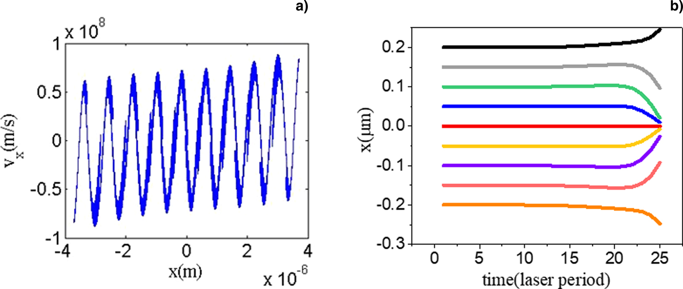
The trajectories of the electrons with initial position at node (x ₀ =  ± 0.2 µm), antinode (x ₀ = 0 µm), near the node (x ₀ =  ± 0.15 µm), near the antinode (x ₀ =  ± 0.05 µm), and the medium (x ₀ =  ± 0.1 µm) are shown in Figure 3b for the case with γ₀ = 2 and a ₀ = 0.68. While traveling through the LSWF, the electrons with initial position at antinode (red line) remain the same position in the x axis during the whole process, because the ponderomotive force is always zero in the antinode plane. Electrons between antinode and node move toward the antinode, while electrons at nodes move inversely to low field regions deviated from the central antinode due to the opposite directions of ponderomotive forces, which are shown in black and orange lines. These results validate the electron convergence at the antinodes planes as described above.

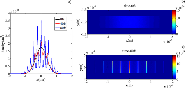
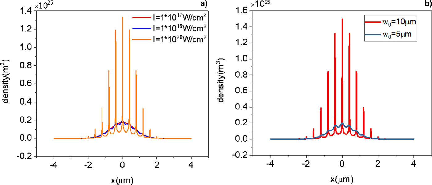
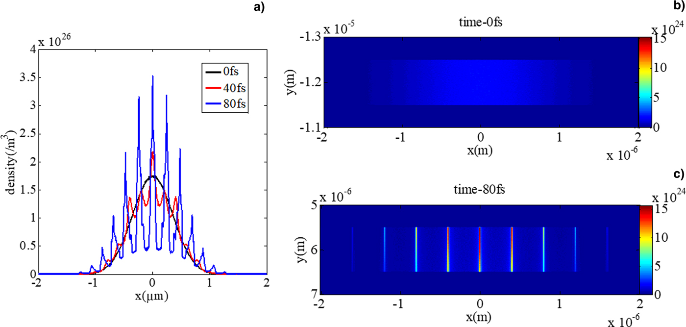
The interaction between electrons and the LSWF is interesting, and it is a potential technology to access electron density modulator. Therefore, the parameters for this electron beam with laser standing waves are worthy of exploration. Figure 4 shows the evolution of the electron density at γ₀ = 2, a ₀ = 0.68. No transverse divergence occurs and the density along the x axis with the initial Gaussian distribution transforms into discrete electron peaks at 40 and 80 fs gradually, as shown in the red and blue lines, respectively. The latter has a higher density in each peak, while the whole structure remains Gaussian. Figure 5a shows the electron density after the interaction for the same high energy of γ₀ = 100 with different laser intensities. At a relatively weak laser intensity of 10¹⁷ W/cm², the final electron distribution through the LSWF is almost unchanged as the same as beginning. By increasing the laser intensity to 10¹⁹ W/cm² (a ₀ = 2.16), a fraction of the electrons begins to move to specific phases. Further increasing the laser intensity to 10²⁰ W/cm², sharp density peaks emerged. These results illustrate that the higher the intensity of the LSWF, the more efficient the effect of electron modulation would be. A threshold intensity exists for the initial energy; however, when using a higher intensity exceeding the threshold value, one could use a shorter beam waist, which will be discussed in the following.

Fig. 4.

Evolution of electron density at γ₀ = 2, a ₀ = 0.68. (a) The y-direction integral curve of electron density distributed in the x axis at different evolution times. (b), (c) The electron-density distribution in simulation box at initial moment and 80 fs, respectively.

Fig. 5.

Electron density along the laser propagating axis after the interaction (a) with different laser intensities for the same γ₀ = 100, w ₀ = 5 μm and (b) with different w ₀ for the same γ₀ = 100, I = 1 × 10¹⁹ W/cm² (a ₀ = 2.16).

The interaction length affects the modulation. The effective modulation length of the LSWF varies with the intensity of the laser. At the same electron initial energy and laser intensity but different beam waists, the electron density after the interaction differs, for example, different laser beam waist diameters of 5 and 10 µm for the same γ₀ = 100, I = 1 × 10¹⁹ W/cm². As Figure 5b shows, the electrons are incompletely separated after the LSWF with a 5-μm beam diameter, accompanied by a high electron density pedestal. However, when doubling the beam diameter to 10 µm, the peak density increases almost 10 times and the density pedestal vanishes but divides into sharp peaks. The whole density remains Gaussian as the initial setting without spatial divergence, causing the electron transverse motion to be limited in the distance of the electron beam length in the x direction. According to Eq. (4), the x motion of electron is simply derived as

(5)$$\eqalign{x = &\displaystyle{{2ke^2a_0^2} \over {{{\rm \varepsilon}} _0m^2c{{\rm \omega}} ^2}} \times \exp \left[ {-\displaystyle{{2(y^2 + z^2)} \over {w_0^2}}} \right] \times sin(2kx) \times \int {[tsin^2({{\rm \omega}} t)]dt} \cr {\rm}={\rm } &\displaystyle{{2ke^2a_0^2} \over {{{\rm \varepsilon}} _0m^2c{{\rm \omega}} ^2}} \times \exp \left[ {-\displaystyle{{2(y^2 + z^2)} \over {w_0^2}}} \right] \times sin(2kx) \cr \times& \left[ {\displaystyle{{t^2} \over 4}-\displaystyle{{tsin(2{{\rm \omega}} t)} \over {4{{\rm \omega}}}} -\displaystyle{{\cos (2{{\rm \omega}} t)} \over {8{{\rm \omega}}^2}}} \right].} $$

The interaction time could be simply estimated as t = w ₀/v ₀, where v ₀ is the initial velocity of electron in the y direction. Therefore, the laser intensity and the beam waist affect the splitting effect together according to Eq. (5). Considering the two factors discussed above, a good electron beam modulator needs to have a long interaction length or sufficiently high field intensity.