



%20--%3e%3c!DOCTYPE%20svg%20PUBLIC%20'-//W3C//DTD%20SVG%201.0//EN'%20'http://www.w3.org/TR/2001/REC-SVG-20010904/DTD/svg10.dtd'%3e%3csvg%20version='1.0'%20id='Layer_1'%20xmlns='http://www.w3.org/2000/svg'%20xmlns:xlink='http://www.w3.org/1999/xlink'%20x='0px'%20y='0px'%20width='64px'%20height='64px'%20viewBox='5.5%20-3.5%2064%2064'%20enable-background='new%205.5%20-3.5%2064%2064'%20xml:space='preserve'%3e%3cg%3e%3ccircle%20fill='%23FFFFFF'%20fill-opacity='0'%20cx='37.785'%20cy='28.501'%20r='28.836'/%3e%3cpath%20fill='%23595959'%20d='M37.441-3.5c8.951,0,16.572,3.125,22.857,9.372c3.008,3.009,5.295,6.448,6.857,10.314%20c1.561,3.867,2.344,7.971,2.344,12.314c0,4.381-0.773,8.486-2.314,12.313c-1.543,3.828-3.82,7.21-6.828,10.143%20c-3.123,3.085-6.666,5.448-10.629,7.086c-3.961,1.638-8.057,2.457-12.285,2.457s-8.276-0.808-12.143-2.429%20c-3.866-1.618-7.333-3.961-10.4-7.027c-3.067-3.066-5.4-6.524-7-10.372S5.5,32.767,5.5,28.5c0-4.229,0.809-8.295,2.428-12.2%20c1.619-3.905,3.972-7.4,7.057-10.486C21.08-0.394,28.565-3.5,37.441-3.5z%20M37.557,2.272c-7.314,0-13.467,2.553-18.458,7.657%20c-2.515,2.553-4.448,5.419-5.8,8.6c-1.354,3.181-2.029,6.505-2.029,9.972c0,3.429,0.675,6.734,2.029,9.913%20c1.353,3.183,3.285,6.021,5.8,8.516c2.514,2.496,5.351,4.399,8.515,5.715c3.161,1.314,6.476,1.971,9.943,1.971%20c3.428,0,6.75-0.665,9.973-1.999c3.219-1.335,6.121-3.257,8.713-5.771c4.99-4.876,7.484-10.99,7.484-18.344%20c0-3.543-0.648-6.895-1.943-10.057c-1.293-3.162-3.18-5.98-5.654-8.458C50.984,4.844,44.795,2.272,37.557,2.272z%20M37.156,23.187%20l-4.287,2.229c-0.458-0.951-1.019-1.619-1.685-2c-0.667-0.38-1.286-0.571-1.858-0.571c-2.856,0-4.286,1.885-4.286,5.657%20c0,1.714,0.362,3.084,1.085,4.113c0.724,1.029,1.791,1.544,3.201,1.544c1.867,0,3.181-0.915,3.944-2.743l3.942,2%20c-0.838,1.563-2,2.791-3.486,3.686c-1.484,0.896-3.123,1.343-4.914,1.343c-2.857,0-5.163-0.875-6.915-2.629%20c-1.752-1.752-2.628-4.19-2.628-7.313c0-3.048,0.886-5.466,2.657-7.257c1.771-1.79,4.009-2.686,6.715-2.686%20C32.604,18.558,35.441,20.101,37.156,23.187z%20M55.613,23.187l-4.229,2.229c-0.457-0.951-1.02-1.619-1.686-2%20c-0.668-0.38-1.307-0.571-1.914-0.571c-2.857,0-4.287,1.885-4.287,5.657c0,1.714,0.363,3.084,1.086,4.113%20c0.723,1.029,1.789,1.544,3.201,1.544c1.865,0,3.18-0.915,3.941-2.743l4,2c-0.875,1.563-2.057,2.791-3.541,3.686%20c-1.486,0.896-3.105,1.343-4.857,1.343c-2.896,0-5.209-0.875-6.941-2.629c-1.736-1.752-2.602-4.19-2.602-7.313%20c0-3.048,0.885-5.466,2.658-7.257c1.77-1.79,4.008-2.686,6.713-2.686C51.117,18.558,53.938,20.101,55.613,23.187z'/%3e%3c/g%3e%3c/svg%3e)
%20--%3e%3c!DOCTYPE%20svg%20PUBLIC%20'-//W3C//DTD%20SVG%201.0//EN'%20'http://www.w3.org/TR/2001/REC-SVG-20010904/DTD/svg10.dtd'%3e%3csvg%20version='1.0'%20id='Layer_1'%20xmlns='http://www.w3.org/2000/svg'%20xmlns:xlink='http://www.w3.org/1999/xlink'%20x='0px'%20y='0px'%20width='64px'%20height='64px'%20viewBox='5.5%20-3.5%2064%2064'%20enable-background='new%205.5%20-3.5%2064%2064'%20xml:space='preserve'%3e%3cg%3e%3ccircle%20fill='%23FFFFFF'%20fill-opacity='0'%20cx='37.637'%20cy='28.806'%20r='28.276'/%3e%3cg%3e%3cpath%20fill='%23595959'%20d='M37.443-3.5c8.988,0,16.57,3.085,22.742,9.257C66.393,11.967,69.5,19.548,69.5,28.5c0,8.991-3.049,16.476-9.145,22.456%20C53.879,57.319,46.242,60.5,37.443,60.5c-8.649,0-16.153-3.144-22.514-9.43C8.644,44.784,5.5,37.262,5.5,28.5%20c0-8.761,3.144-16.342,9.429-22.742C21.101-0.415,28.604-3.5,37.443-3.5z%20M37.557,2.272c-7.276,0-13.428,2.553-18.457,7.657%20c-5.22,5.334-7.829,11.525-7.829,18.572c0,7.086,2.59,13.22,7.77,18.398c5.181,5.182,11.352,7.771,18.514,7.771%20c7.123,0,13.334-2.607,18.629-7.828c5.029-4.838,7.543-10.952,7.543-18.343c0-7.276-2.553-13.465-7.656-18.571%20C50.967,4.824,44.795,2.272,37.557,2.272z%20M46.129,20.557v13.085h-3.656v15.542h-9.944V33.643h-3.656V20.557%20c0-0.572,0.2-1.057,0.599-1.457c0.401-0.399,0.887-0.6,1.457-0.6h13.144c0.533,0,1.01,0.2,1.428,0.6%20C45.918,19.5,46.129,19.986,46.129,20.557z%20M33.042,12.329c0-3.008,1.485-4.514,4.458-4.514s4.457,1.504,4.457,4.514%20c0,2.971-1.486,4.457-4.457,4.457S33.042,15.3,33.042,12.329z'/%3e%3c/g%3e%3c/g%3e%3c/svg%3e)
1. Introduction
The scattering of acoustic waves into Kelvin–Helmholtz instability waves at the nozzle-exit section of jets via the receptivity process, a process by which external disturbances trigger the growth of instabilities in a shear flow, is a key process in several jet flow configurations. For instance, it plays an important role when jets are excited by acoustic waves to control their turbulent development or to reduce their radiated noise, as was the case in Sato (Reference Sato1960), Crow & Champagne (Reference Crow and Champagne1971) and Kibens (Reference Kibens1980), and when aeroacoustic resonance loops establish in the jet flow. On the latter issue, the receptivity process has been recognized to close the feedback loops generating intense acoustic tonal components in screeching and impinging jets for more than seventy years since the pioneering studies of Powell (Reference Powell1953a,Reference Powellb), as reported in the reviews of Raman (Reference Raman1999) and Edgington-Mitchell (Reference Edgington-Mitchell2019). Recently, it was also shown in Bogey (Reference Bogey2022a) to promote the development of instability waves near the nozzle of non-screeching jets with fully laminar nozzle-exit conditions in the specific frequency ranges of the upstream-propagating guided jet waves essentially confined in the flow, described for the first time by Tam & Hu (Reference Tam and Hu1989) and later by Towne et al. (Reference Towne, Cavalieri, Jordan, Colonius, Schmidt, Jaunet and Brès2017) and Bogey (Reference Bogey2021), among others.
The efficiency of the receptivity process in shear flows has been investigated in the past by several researchers using mathematical methods. For instance, Tam (Reference Tam1978) studied the excitation of instability waves in two-dimensional subsonic compressible shear layers of finite thickness by a beam of sound waves, in the absence of a scattering surface, using Green's functions. The effectiveness of the excitation was found to depend on the angle of incidence and the width of the wave beam, and to increase with the Mach number. In particular, it turned out to be greatest for a narrow beam of waves aiming at a angle to the flow direction decreasing with the Mach number, over a range between 30 $^\circ$ and 80
 $^\circ$ for Mach number 0.6, for instance. The receptivity process was also investigated in a shear layer of a vortex-sheet type behind an infinitely thin flat plate by Bechert (Reference Bechert1988), and by Kerschen (Reference Kerschen1996) and Li & Lyu (Reference Li and Lyu2023) using the Wiener–Hopf technique, just to mention a few. Transfer functions describing the receptivity to acoustic disturbances were determined. Recently, resolvent analyses were also conducted from the mean flow fields of jets to seek the sets of external forcing and response modes that are optimal with respect to the energetic gain between them. They were applied to subsonic and supersonic jets in Schmidt et al. (Reference Schmidt, Towne, Rigas, Colonius and Brès2018) and Pickering et al. (Reference Pickering, Rigas, Nogueira, Cavalieri, Schmidt and Colonius2020).
Results on the receptivity of a shear layer to acoustic waves behind a trailing edge or a nozzle lip have also been obtained using other approaches. Barone & Lele (Reference Barone and Lele2005) examined the receptivity of compressible supersonic mixing layers downstream of a splitter plate of finite width capped with a rounded trailing edge using an adjoint analysis. Receptivity was noted to be a function of the source type, frequency and location. Imai & Asai (Reference Imai and Asai2009) explored experimentally the receptivity of a laminar shear layer separating from a rear edge of a boundary-layer plate. They quantified the dependency of the receptivity coefficient on the rear-edge curvature and on the frequency of the acoustic disturbances. Karami et al. (Reference Karami, Stegeman, Ooi, Theofilis and Soria2020) studied numerically the receptivity of two under-expanded supersonic impinging jet flows emanating from an infinite-lipped nozzle by introducing acoustic pulses in the mean flow fields obtained by large-eddy simulations (LES). The effects of the angle of incidence with respect to the jet centreline, of the azimuthal mode number and the frequency of the waves hitting the nozzle, and of the nozzle-to-plate distance were addressed by computing transfer functions between the input acoustic signals and the output vortical signals at the nozzle lip. For a nozzle-to-plate distance of five jet diameters, in particular, the jet receptivity to acoustic disturbances was found to be high for incidence angles between  $15^{\circ }$ and
 $50^{\circ }$, and for angles greater than
 $80^{\circ }$ from the jet centreline. In their theoretical work, Mancinelli et al. (Reference Mancinelli, Jaunet, Jordan and Towne2021) also proposed an approach to identify the reflection coefficients of the upstream-propagating waves at the nozzle exit to model the resonance mechanisms in screeching jets.
For impinging jets, the frequencies and strengths of the feedback loops are sensitive to the external geometry of the nozzle and to the presence of reflective surfaces upstream of the jets, as was illustrated in the experiments of Weightman et al. (Reference Weightman, Amili, Honnery, Edgington-Mitchell and Soria2019) and in the LES of Karami & Soria (Reference Karami and Soria2021). In Weightman et al. (Reference Weightman, Amili, Honnery, Edgington-Mitchell and Soria2019), intriguingly, a switch of the dominant azimuthal modes was observed between thin- and infinite-lipped nozzles. It was attributed to the fact that the closure path in the thin-lip case involves a reflection of the acoustic waves from the outer surface of the nozzle base back to the nozzle lip. For screeching jets, the screech mode staging, frequencies and amplitudes can also change with the nozzle-lip geometry and roughness, as was highlighted very recently in Alapati & Srinivasan (Reference Alapati and Srinivasan2024). In particular, the intensities of the feedback loops have been known since the work of Powell (Reference Powell1954) to depend on the thickness of the nozzle lip, on which the coupling between the upstream-propagating acoustic waves and the near-nozzle shear-layer instability waves occurs. Although somewhat mode-dependent, the inclusion of a thicker lip usually results in stronger screech tones, whereas very thin lips may lead to screech cessation. These trends were observed in the experiments of Norum (Reference Norum1983), Ponton & Seiner (Reference Ponton and Seiner1992) and Raman (Reference Raman1997), and in the numerical study of Shen & Tam (Reference Shen and Tam2000). They strongly suggest that increasing the nozzle-lip thickness results in a greater efficiency of the receptivity process. The gain in efficiency is, however, difficult to quantify because thickening the nozzle lip alters the entrainment field in the near-nozzle region, which most likely also affects the feedback loop properties.
Therefore, the increase of the efficiency of the receptivity of jets to acoustic disturbances as the nozzle lip is thicker is investigated in the present paper using numerical simulations. For that purpose, acoustic pulses are introduced in isothermal round free jets at Mach numbers ranging from 0.4 up to 1.3, issuing from straight pipe nozzles with lips of different thicknesses. The latter vary between  $\delta _{lip} = 0.01r_0$ and
 $\delta _{lip} = 0.93r_0$, where
 $r_0$ is the nozzle radius. At the initial time of the simulations, the jet flow is modelled by specifying a boundary-layer velocity profile all over the computational domain, both upstream and downstream of the nozzle exit. Acoustic pulses of very low amplitude are placed outside the nozzle, inside the flow on the jet axis, or outside with angles of incidence between
 $5^{\circ }$ and
 $90^{\circ }$ with respect to the downstream direction, in order to create linear sound waves in the domain. These waves travel up to the nozzle lip where they are reflected, which leads to the generation of instability waves growing exponentially in the jet mixing layers. In this work, the gain in efficiency of the jet receptivity with the increase of the nozzle-lip thickness will be determined directly from the amplitude of the instability waves measured near the nozzle. It will be characterized by power laws. The influence of the location of the acoustic pulse inside or outside the jet flow, of the angle of incidence of the acoustic disturbances on the nozzle-lip section, of the azimuthal mode number of the disturbances, of the pulse spatial extent, and of the shape of the boundary-layer profile, will then be discussed. Given the Mach number range considered, the effects of the jet Mach number could also be pointed out.
The paper is organized as follows. The characteristics of the jet flows and of the acoustic pulses, the simulation parameters and the procedure used to calculate the gain in efficiency of the jet receptivity are presented in § 2. The results obtained for a pulse inside the jet flow and for pulses outside the flow, for the axisymmetric azimuthal mode but also for non-axisymmetric ones, are provided in § 3. Concluding remarks are given in § 4. Finally, results obtained for pulses of different half-widths and with boundary-layer profiles of different shapes are reported in two appendices.
2. Parameters
2.1. Jet flow and acoustic pulse characteristics
In this study, numerical simulations are performed for isothermal round free jets at Mach numbers  $M=u_j/c_a=0.4$,
 $0.6$,
 $0.9$ and
 $1.3$, and at Reynolds number
 $Re_D=u_jD/\nu =10^5$, where
 $u_j$,
 $c_a$,
 $D$ and
 $\nu$ are the jet velocity, the speed of sound in the ambient medium, the nozzle diameter and the kinematic molecular viscosity, respectively. The jets originate from a pipe nozzle of radius
 $r_0=D/2$ and length
 $2 r_0$ into a medium at ambient temperature and pressure
 $T_a=293$ K and
 $p_a=10^5$ Pa. The nozzle ends at
 $z=0$ in a lip with a straight section of thickness
 $\delta _{lip}$, and sharp corners.
At initial time  $t=0$ of the simulations, a Blasius laminar boundary-layer profile is imposed for the axial velocity
 $u_z$ from the pipe inlet down the outflow boundary (Bogey & Bailly Reference Bogey and Bailly2010), i.e. both upstream and downstream of the nozzle exit. It is referred to as the BL profile (Bogey & Sabatini Reference Bogey and Sabatini2019) in what follows. For the present jets, the profile has a thickness of
 $0.1r_{0}$, as represented in figure 1, yielding a momentum thickness
 $\delta _{\theta }=0.012 r_0$ and a Reynolds number
 $Re_{\theta }=u_j\delta _{\theta }/\nu =600$. Radial and azimuthal velocities are set to zero, pressure is equal to
 $p_a$, and temperature is determined by a Crocco–Busemann relation.
The BL boundary-layer profile of axial velocity  $u_z/u_j$ for the present jets.

These flow conditions were previously specified in the nozzle of untripped jets computed by LES (Bogey Reference Bogey2021, Reference Bogey2022a). In Bogey (Reference Bogey2022a), in particular, linear stability analyses (Michalke Reference Michalke1984) were performed from the LES mean flow profiles downstream of the nozzle using a procedure solving the compressible Rayleigh equation (Bogey & Sabatini Reference Bogey and Sabatini2019), in which viscosity is not taken into account given that  $Re_{\theta } > 500$ (Morris Reference Morris1983, Reference Morris2010). This procedure is applied to the boundary-layer profiles in this study. The instability growth rates
 $-{\rm Im}(k_z)r_0$ obtained for the azimuthal modes
 $n_{\theta }=0$ for
 $M=0.6$,
 $n_{\theta }=0-2$ for
 $M=0.9$, and
 $n_{\theta }=0$ for
 $M=1.3$, where
 $k_z$ is the complex wavenumber of the instability waves, are represented in figures 2(a–c) as functions of
 $St_{\theta }=f\delta _{\theta }/u_j$, where
 $f$ is the frequency. With increasing Mach number, the amplification rates and the most unstable Strouhal numbers decrease, as expected (Michalke Reference Michalke1984; Morris Reference Morris2010). For
 $M=0.9$, the growth rates for the four azimuthal modes are very similar, the strongest ones being found for
 $n_{\theta }=0$. For comparison, the instability growth rates calculated in Bogey (Reference Bogey2022a) at
 $z=0.6r_0$ for
 $n_{\theta }=0\unicode{x2013}2$ for a jet at
 $M=0.9$ with the same nozzle-exit profiles as the jets in this work are also shown. Again, they do not depend significantly on the mode number. The highest growth rates are reached at
 $St_{\theta }=0.013$ for
 $n_{\theta }=0$. At this frequency, the phase velocity of the instability waves was noted to be equal to
 $0.5u_j$.
Instability growth rates obtained for (a)  $M=0.6$, (b)
 $M=0.9$ and (c)
 $M=1.3$ as functions of
 $St_{\theta }$, (solid lines) for the BL boundary-layer profile and (dashed lines) for the mean flow profiles at
 $z=0.6r_0$ for an untripped jet (Bogey Reference Bogey2022a): (black)
 $n_{\theta }=0$, (red)
 $n_{\theta }=1$ and (blue)
 $n_{\theta }=2$.

In this study, four nozzle-lip thicknesses are considered, as shown in figures 3(a–d). They vary approximately from  $\delta _{lip} = 0.01r_0$ up to
 $\delta _{lip} = 0.9r_0$, following a geometric progression with a common ratio of 4. More precisely, they are equal to
 $\delta lip(0)/4=0.014r_0$,
 $\delta lip(0)=0.058r_0$,
 $4 \delta lip(0)=0.23r_0$ and
 $16\delta lip(0)=0.93r_0$, where
 $\delta lip(0)$ is the value in several former jet LES (Bogey Reference Bogey2018, Reference Bogey2021, Reference Bogey2022a; Bogey & Sabatini Reference Bogey and Sabatini2019). In what follows, they will be referred to as dlip1, dlip2, dlip3 and dlip4, from the thinnest to the thickest lips.
Representations of the nozzle lips, the positions of the acoustic pulses and the geometrical parameters in the present study: (a) dlip1, (b) dlip2, (c) dlip3 and (d) dlip4.

To generate pressure waves in the computational domain, an acoustic pulse is added onto the mean flow field at  $t=0$. The pulse is introduced outside the nozzle at a distance
 $d=2r_0$ from the nozzle-lip inner corner at
 $z=0$ and
 $r=r_0$, for angles
 $\varphi =-30^{\circ }$,
 $5^{\circ }$,
 $15^{\circ }$,
 $30^{\circ }$,
 $60^{\circ }$,
 $75^{\circ }$ and
 $90^{\circ }$ between the line
 $r=r_0$ and the line passing through the inner corner and the pulse position. Thus the pulse is located inside the flow on the jet axis jet in the first case, and outside the flow in the six others. The pulse positions are denoted as
 $P_{axis}$,
 $P_{5^{\circ }}$,
 $P_{15^{\circ }}$,
 $P_{30^{\circ }}$,
 $P_{60^{\circ }}$,
 $P_{75^{\circ }}$ and
 $P_{90^{\circ }}$, respectively. They are represented in figures 3(a–d) and in the left-hand columns of figures 4, 5, 8, 9 and 10 in § 3, and of figures 20 and 21 in Appendix A.
Pressure fluctuations obtained with dlip1 for an axisymmetric pulse with  $b=0.2r_0$ located at
 $\bullet$
 $P_{axis}$ for (a–e)
 $M=0.4$, (f–j)
 $M=0.6$, (k–o)
 $M=0.9$ and (p–t)
 $M=1.3$, between
 $t=t_{d/c_a}$ and
 $t_{d/c_a}+4r_0/u_j$ in increments of
 $r_0/u_j$, from left to right. The colour scale levels range from
 $-0.06A$ to
 $0.06A$, from blue to red.

Pressure fluctuations obtained with dlip4 for an axisymmetric pulse with  $b=0.2r_0$ located at
 $\bullet$
 $P_{axis}$; same jet Mach numbers, times and colour scale as in figure 4.

The pulse is axisymmetric in most cases, but is non-axisymmetric and characterized by an azimuthal mode number  $n_{\theta }=1,2$ in a few. Axisymmetric pulses as well as pulses for
 $n_{\theta }=1,2$ were also considered in the receptivity study of Karami et al. (Reference Karami, Stegeman, Ooi, Theofilis and Soria2020) for supersonic impinging jets. Overall, similar results were obtained in the three cases. In an azimuthal section, the pulse is Gaussian and has a half-width
 $b=0.2r_0$. The amplitude of the pulse
 $A$ is set to the very low value
 $A=10^{-5} p_a$ to avoid nonlinear effects during the propagation of the acoustic waves and during the growth of the instability waves just downstream of the nozzle. The absence of nonlinear effects on the present results was verified by performing simulations with
 $A=10^{-6} p_a$. The solutions obtained with
 $A=10^{-5} p_a$ and
 $A=10^{-6} p_a$ were found to be superimposed.
The different cases studied in the main body of this paper, each using the four nozzle-lip thicknesses, are summarized in table 1. For the four Mach numbers, simulations are performed with axisymmetric acoustic pulses for the seven pulse positions defined above. For  $M=0.9$, non-axisymmetric pulses with azimuthal mode numbers
 $n_{\theta }=1, 2, 3$ are also considered at the positions
 $P_{15^{\circ }}$. Finally, additional simulations for
 $M=0.9$ are presented in two appendices. They deal with axisymmetric pulses of half-widths
 $b=0.1r_0$ and
 $0.4r_0$ located at
 $P_{axis}$ and
 $P_{30^{\circ }}$ in Appendix A, and with an axisymmetric pulse placed at
 $P_{30^{\circ }}$ outside two jets with non-laminar boundary-layer mean-velocity profiles in Appendix B.
Jet boundary layers and Mach numbers, azimuthal mode numbers, half-widths and positions of the acoustic pulses.

For each of the 16 sets of ( $M$,
 $\delta _{lip}$) and 8 sets of (non-laminar boundary-layer type,
 $\delta _{lip}$), simulations are also made without pulse, leading to a total number of 168 computations. The results obtained with and without pulse are subtracted to remove from the solutions the initial transient of the jet flow and the fluctuations that would be obtained naturally without pulse. This allows us to isolate and extract the response of the jet flow to the acoustic disturbances, which will be used to quantify the efficiency of this receptivity process as explained in § 2.3.
2.2. Numerical methods and parameters
The computations are carried out by solving the three-dimensional compressible Navier–Stokes equations in cylindrical coordinates  $(r,\theta,z)$ using the same framework as in recent jet simulations (Bogey Reference Bogey2018, Reference Bogey2021, Reference Bogey2022a,Reference Bogeyb; Bogey & Sabatini Reference Bogey and Sabatini2019). The axis singularity is taken into account by the method of Mohseni & Colonius (Reference Mohseni and Colonius2000). In order to alleviate the time-step restriction near the cylindrical origin, the derivatives in the azimuthal direction around the axis are calculated at resolutions coarser than permitted by the grid (Bogey, de Cacqueray & Bailly Reference Bogey, de Cacqueray and Bailly2011). Fourth-order eleven-point centred finite differences are used for spatial discretization, and a second-order six-stage Runge–Kutta algorithm is implemented for time integration (Bogey & Bailly Reference Bogey and Bailly2004). A sixth-order eleven-point centred filter (Bogey, de Cacqueray & Bailly Reference Bogey, de Cacqueray and Bailly2009) is applied explicitly to the flow variables every time step to remove grid-to-grid oscillations. Non-centred finite differences and filters are also used near the pipe walls and the grid boundaries (Berland et al. Reference Berland, Bogey, Marsden and Bailly2007). At the boundaries, the radiation conditions of Tam & Dong (Reference Tam and Dong1996) are applied with the addition of sponge zones based on grid stretching at the lateral and outflow boundaries.
Four grids are used, depending on the nozzle-lip thickness. They derive from the one constructed in a grid-sensitivity study for jet LES (Bogey Reference Bogey2018). They are identical to each other in the radial direction between  $r=0$ and
 $r=r_0$, and in the azimuthal and axial directions along which there are
 $N_{\theta }=256$ and
 $N_z=859$ points, respectively. Excluding the 30-point and 100-point lateral and outflow sponge zones, they all extend radially out to
 $r=L_r = 4r_0$ and axially down to
 $z=L_z=6r_0$. In the radial direction, there are 96 points between
 $r=0$ and
 $r=r_0$. The mesh spacing
 $\Delta r$ is equal to
 $0.014r_0$ on the jet axis, to
 $0.0036r_0$ between
 $r=r_0$ and
 $r=r_0+\delta _{lip}$, and to
 $0.033r_0$ at
 $r=L_r$. As the value of
 $\delta _{lip}$ increases, the grid spacing at
 $r=3r_0$ decreases from
 $\Delta r=0.024r_0$ for dlip1 down to
 $\Delta r=0.016r_0$ for dlip4, and the number of points varies between
 $N_r=336$ and
 $N_r=588$. In the axial direction, there are 169 points between
 $z=-2r_0$ and
 $z=0$ along the pipe nozzle. The mesh spacing
 $\Delta z$ is minimum and equal to
 $0.0072r_0$ between
 $z=-r_0$ and
 $z=0$. Farther downstream, it increases at a constant stretching rate and reaches
 $\Delta z=0.014r_0$ at
 $z=L_z$. As a result, the acoustic pulses imposed at
 $t=0$ are well discretized, and all contain more than 6.7 grid points in their half-widths. This value corresponds to the ratio
 $b/\Delta r$ obtained in one of the cases considered in Appendix A, for
 $b=0.1r_0$ and the grid spacing
 $\Delta r=0.015r_0$ at position
 $P_{30^{\circ }}$ for dlip1.
Finally, the simulations are performed with an OpenMP-based in-house solver on single nodes with 16 cores, between  $t=0$ and
 $t=t_{max}$ using a time step
 $\Delta t=0.7 \times \Delta r(r=r_0)/c_a$, ensuring numerical stability in all cases. Among the data stored, pressure is recorded in the azimuthal plane at
 $\theta =0$ at a sampling frequency corresponding to Strouhal number
 $St_D=fD/u_j=6.4$, in particular at seven times varying between
 $t_{d/c_a}=d/c_a$ and
 $t_{max}=t_{d/c_a}+6r_0/u_j$ in increments of
 $r_0/u_j$. The number of iterations ranges from 2608 for
 $M=1.3$ up to 6702 for
 $M=0.40$. Thus the total cost of the study is of the order of 60 000 CPU hours.
2.3. Definition of the gain in receptivity efficiency
In this work, the objective is not to investigate the efficiency of the receptivity process of the jets to the acoustic disturbances. This efficiency depends indeed on several parameters such as the jet Mach number, the nozzle-exit boundary-layer velocity profile, the angle of incidence, and the wavelength of the acoustic disturbances and the nozzle-lip geometry. It can be quantified by computing transfer functions between input and output signals, as performed in the simulations of Karami et al. (Reference Karami, Stegeman, Ooi, Theofilis and Soria2020) and in the jet control experiments of Maia et al. (Reference Maia, Jordan, Cavalieri, Martini, Sasaki and Silvestre2021), for instance. The calculation of these functions may, however, be limited by the spatial and temporal resolutions and durations of the signals, especially when the input disturbances result from acoustic pulses. Moreover, even if the output signals are acquired at a point very close to the nozzle, they are amplified and distorted during the propagation of the shear-layer instability waves from the nozzle to that point. This will necessarily affect the transfer functions computed between the input and output signals.
The aim here is rather to determine the increase of the efficiency of the receptivity process as the nozzle lip is thicker. This can be done directly from the amplitudes of the instability waves growing downstream of the nozzle-lip inner corner after the acoustic waves hit the nozzle, without computing transfer functions. In practice, for a given case, the gain in receptivity efficiency between the simulations carried out using the nozzle-lip thicknesses  $\delta _{lip}$ and dlip1 is evaluated as
 \begin{equation} G(\delta_{lip}) = \frac{\max (\,p'(r=r_0,t=t_{z_{WP}},\delta_{lip}))}{\max(\,p'(r=r_0,t=t_{z_{WP}},dlip1))}, \end{equation}
where the pressure fluctuation  $p'$ is unusually defined as the difference between the pressure values obtained with and without pulse, Thus it corresponds to the response of the jet flow to the acoustic disturbances as mentioned in § 2.1. No azimuthal decomposition of the pressure fields is performed in this study because the acoustic disturbances and the resulting instability waves have the same azimuthal organization. This has been checked in preliminary tests. Finally, the maximum value of
 $p'$ is used to estimate the amplitude of the instability waves, because in most cases it is higher, in absolute value, than the minimum value, as will be exemplified later in figures 6, 11, 18 and 22. Similar trends would, however, be obtained using the minimum value of
 $p'$ to compute the gain
 $G$.
Pressure fluctuations obtained at  $r=r_0$ and
 $t=t_{z_{WP}}$ for an axisymmetric pulse with
 $b=0.2r_0$ located at
 $P_{axis}$ for
 $M=0.9$: (black) dlip1, (red) dlip2, (blue) dlip3 and (green) dlip4.

The time  $t_{z_{WP}}$ is taken slightly after the acoustic waves reach the nozzle lip, when the instability wave excited by the reflected waves typically lies between
 $z=0.5r_0$ and
 $z=r_0$. At that time, the amplitude of the instability wave is sufficiently high to overcome that of the possibly remaining acoustic pressure waves, but is still low to grow exponentially due to a linear mechanism. The time
 $t_{z_{WP}}$ is estimated in each case, so that it coincides with the time when the peak amplitude of the shear-layer instability wave packet at
 $r=r_0$ arrives at the axial position
 $z_{WP}$. Thus the gain
 $G$ is calculated from instability waves located at the same distances from the nozzle exit. The values of
 $z_{WP}$ chosen in this study are reported in table 2. They vary with the jet Mach number and with the position of the pulse inside or outside of the jet to avoid in all cases, at time
 $t_{z_{WP}}$, the presence of strong acoustic waves at
 $z=z_{WP}$ where the amplitude of the instability waves is measured. When this condition is satisfied, the gain in receptivity efficiency has been found not to depend significantly on
 $z_{WP}$.
Axial positions  $z_{WP}$ where the peak amplitudes of the shear-layer instability wave packets are measured.

For a given Mach number and a given pulse, all the parameters in the simulations are identical except for the nozzle-lip thickness. Furthermore, the propagation of the incident acoustic waves and the growth of the instability waves between  $z=0$ and
 $z=z_{WP}$ are both governed by linear mechanisms. Therefore, the variations of the amplitudes of the instability waves at
 $z=z_{WP}$ with the nozzle-lip thickness, hence the values of the gain
 $G$, can result only from differences in the efficiency of the scattering of the acoustic disturbances into instability waves at the nozzle lip.
In what follows, the increase of the receptivity efficiency will be characterized systematically by approximating the values of  $G(\delta _{lip})$ obtained for dlip1, dlip2, dlip3 and dlip4 by power functions using a curve-fitting method, such as
 \begin{equation} G(\delta_{lip}) \simeq K\left(\frac{\delta_{lip}}{dlip1}\right)^e, \end{equation}
where the amplitude  $K$ and the exponent
 $e$ are real numbers. Given the normalization of the gain
 $G$ imposing
 $G(dlip1)=1$, only the values of the exponent
 $e$ of the power law will be of interest.
3. Results
The gain in receptivity efficiency is investigated first when the pulse is initially inside the jet, then when it is located outside. In the first case, the disturbances hitting the nozzle lip are upstream-propagating pressure waves that can be more or less confined in the jet flow, as happens for the guided jet waves (Tam & Hu Reference Tam and Hu1989; Towne et al. Reference Towne, Cavalieri, Jordan, Colonius, Schmidt, Jaunet and Brès2017; Jordan et al. Reference Jordan, Jaunet, Towne, Cavalieri, Colonius, Schmidt and Agarwal2018; Bogey Reference Bogey2021) recently shown to play a key role in the occurrence of resonance phenomena in jets (Edgington-Mitchell Reference Edgington-Mitchell2019). In the second case, they are free-stream sound waves. The pulse has a half-width  $b=0.2r_0$ in all the simulations in this section. It is axisymmetric in §§ 3.1 and 3.2, and can be non-axisymmetric in § 3.3.
Results obtained for pulses with half-widths  $b=0.1r_0$ and
 $b=0.4r_0$ and using non-laminar boundary-layer mean-velocity profiles for Mach number
 $M=0.9$ are provided in Appendices A and B. They are very similar to those reported in this section. This suggests that the increase of the receptivity efficiency does not depend much on the spatial extent of the acoustic pulse or on the shape of the boundary-layer velocity profile.
3.1. Acoustic pulse inside the jet
The pressure fields obtained in a  $(z,r)$ cross-section for a pulse located inside the jet at
 $P_{axis}$ with the thinnest and the thickest nozzle lips are represented in figures 4 and 5 at five times between
 $t_{d/c_a}$ and
 $t_{d/c_a}+4r_0/u_j$, from left to right. In both figures, the jet Mach number increases from 0.4 up to 1.3, from top to bottom. Since the pressure fields are axisymmetric, only the upper part with
 $r\geq 0$ is shown.
At  $t=t_{d/c_a}$, in all the left-hand pictures, a wave has been transmitted to the outside of the flow through the jet shear layer, and radiates in the ambient medium in all directions. It is extended into the jet by an oblique wave propagating in the upstream direction at a phase velocity close to the ambient sound speed. This wave moving against the flow in the potential jet core can be observed easily, for example, in figures 4(l) and 5(l) for
 $M=0.9$, but also in figures 4(q,r) and 5(q,r) for
 $M=1.3$. In the supersonic case, it forms an angle with respect to the upstream direction in agreement with the angle
 $\psi$ predicted by Tam & Hu (Reference Tam and Hu1989) for guided jet waves with subsonic phase velocities in a supersonic jet. It also looks like the upstream-propagating waves extracted by Bogey & Gojon (Reference Bogey and Gojon2017) in the potential core of supersonic impinging jets generating tones. Therefore, the oblique wave inside the present jets most likely corresponds to a guided jet wave resulting from the reflection of the incident pulse on the shear layer, according to the mechanism described theoretically in Nogueira et al. (Reference Nogueira, Cavalieri, Martini, Towne, Jordan and Edgington-Mitchell2024) by solving an acoustic-scattering problem for planar vortex sheets.
The pressure disturbances travelling upstream in the shear-layer region hit the nozzle lip slightly after  $t_{d/c_a}$ for
 $M=0.4$, between
 $t_{d/c_a}$ and
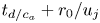 $t_{d/c_a}+r_0/u_j$ for
 $M=0.6$, slightly before
 $t_{d/c_a}+r_0/u_j$ for
 $M=0.9$ and
 $t_{d/c_a}+2r_0/u_j$ for
 $M=1.3$. They are clearly reflected back by the nozzle for dlip4, but this is not obvious for dlip1, e.g. in figures 4(b) and 5(b) for
 $M=0.4$. An acoustic wave is also found to propagate inside the jet in the upstream direction with a phase speed of
 $u_j-c_a$ for the three subsonic Mach numbers, but not for the supersonic one, as expected. This wave can be seen upstream of the pulse position in the left-hand pictures of the figures for the subsonic cases.
After the upstream-propagating pressure wave has impacted the nozzle, an instability wave packet develops downstream of the nozzle-lip inner corner. For a time delay of approximately  $2r_0/u_j$ after the impact, the wave packet is located near
 $z=r_0$; see figures 5(n,t), for instance. This location is consistent with a convection velocity close to
 $0.5u_j$. For a given Mach number, the wave packet appears stronger for dlip4 than for dlip1. For
 $M=1.3$, in particular, it is hardly detectable in figure 4(t) for dlip1, but is well visible in figure 5(t) for dlip4.
To illustrate the variations of the wave-packet properties with the nozzle-lip thickness, the pressure fluctuations obtained at  $r=r_0$ and
 $t=t_{z_{WP}}$ for
 $M=0.9$ with the four lip thicknesses are represented in figure 6. In the four cases, a wave packet is found to peak at the position
 $z=z_{WP}=0.9r_0$ specified in table 2. As the nozzle-lip thickness is larger, its shape does not seem to change much, but its amplitude increases significantly. Consequently, the peak pressure values obtained for dlip2, dlip3 and dlip4 are 1.6, 3.1 and 4.7 higher than that for dlip1.
Regarding the spectral content of the instability wave packet, its oscillatory part exhibits a wavelength close to  $0.5r_0$. Assuming that the wave packet is convected a phase velocity of
 $0.5u_j$, this yields a Strouhal number
 $St_{\theta }=f\delta _{\theta }/u_j=0.012$. This value is consistent with
 $St_{\theta }=0.013$ predicted in Bogey (Reference Bogey2022a) using linear stability analysis for the most amplified instability waves just downstream of the nozzle for a jet at
 $M=0.9$ with a BL exit profile of thickness
 $0.1r_0$ like the present jets, as shown in figure 2(b) in § 2.1.
Moreover, the times  $t_{WP}$ when the wave packets peak at
 $z=z_{WP}$ are all very close to
 $t_{d/c_a}+2.86 r_0/u_j$ in the four cases, differing by less than
 $0.02r_0/u_j$ from each other. A similar result is noted for the three other Mach numbers. This suggests that the thickening of the nozzle lip does not generate any significant additional time delay during the receptivity process when the acoustic source is located inside the jet flow.
Finally, the gains in receptivity efficiency  $G$ obtained for the four Mach numbers as a thicker nozzle lip is used, calculated from the wave packet amplitudes at
 $t=t_{z_{WP}}$ according to (2.1), are plotted in figure 7 as a function of
 $\delta _{lip}/r_0$. They are very similar for
 $M=0.4$ and
 $M=0.6$, but are stronger for higher Mach numbers. Between the thinnest and thickest nozzle lips, for example, they reach values 2.9 for
 $M=0.4$, 3.1 for
 $M=0.6$, 4.7 for
 $M=0.9$, and 5.6 for
 $M=1.3$. For each Mach number, in addition, the variations of the gains with
 $\delta _{lip}$ are shown to approximately follow a power law. The exponents of the corresponding power functions (2.2) determined by curve fitting are
 $e=0.26$, 0.28, 0.36 and 0.42 from
 $M=0.4$ up to
 $M=1.3$. These values reflect the fact that the efficiency of the jet receptivity process increases more rapidly with the nozzle-lip thickness for a higher Mach number. The reason for this will be discussed in the next section.
Variations with  $\delta _{lip}/r_0$ of the gain in receptivity efficiency
 $G$ obtained for an axisymmetric pulse with
 $b=0.2r_0$ located at
 $P_{axis}$ for (black)
 $M=0.4$, (red)
 $M=0.6$, (blue)
 $M=0.9$ and (green)
 $M=1.3$; (circles) simulations and (lines) power functions.

3.2. Acoustic pulse outside the jet
For a pulse located outside the jet, different trends are observed depending on the angle of incidence of the acoustic waves, for  $\varphi \leq 60^{\circ }$ and for
 $\varphi \geq 75^{\circ }$. To highlight this, pressure fields are first shown for pulses located at
 $P_{30^{\circ }}$ and at
 $P_{75^{\circ }}$.
The pressure fluctuations obtained for a pulse at  $P_{30^{\circ }}$ with dlip1 and dlip4 are represented in figures 8 and 9, respectively, at four times between
 $t_{d/c_a}$ and
 $t_{d/c_a}+3r_0/u_j$, from left to right, and for jet Mach numbers increasing from 0.4 up to 1.3, from top to bottom. At
 $t=t_{d/c_a}$, the acoustic wave generated by the pulse has reached the nozzle lip, as expected. As was noted for the pulse located inside the jet in the previous section, a wave is clearly reflected by the nozzle in the downstream direction for dlip4 in figure 9 but not for dlip1 in figure 8. At subsequent times, an instability wave packet appears downstream of the nozzle-lip inner corner, and grows in amplitude as it is convected by the jet flow. For each Mach number, at a given time, the wave packet is at a similar location for the two nozzle lips, but is stronger for the thickest one. The strengthening of the wave packet for a thicker nozzle lip seems particularly marked at a high Mach number. This can be seen, for instance, by comparing the magnitudes of the instability waves emerging near
 $z=r_0$ in figures 8(o) and 9(o) for
 $M=1.3$.
Pressure fluctuations obtained with dlip1 for an axisymmetric pulse with  $b=0.2r_0$ located at
 $\bullet$
 $P_{30^{\circ }}$ for (a–d)
 $M=0.4$, (e–h)
 $M=0.6$, (i–l)
 $M=0.9$ and (m–p)
 $M=1.3$, between
 $t=t_{d/c_a}$ and
 $t_{d/c_a}+3r_0/u_j$ in increments of
 $r_0/u_j$, from left to right. The colour scale levels range from
 $-0.5A$ to
 $0.5A$, from blue to red.

Pressure fluctuations obtained with dlip4 for an axisymmetric pulse with  $b=0.2r_0$ located at
 $\bullet$
 $P_{30^{\circ }}$; same jet Mach numbers, times and colour scale as in figure 8.

The pressure fields obtained for a pulse located at  $P_{75^{\circ }}$ with dlip1 and dlip4 for
 $M=0.9$ are displayed in figures 10(a–d) and 10(e–h), respectively, at four times between
 $t_{d/c_a}$ and
 $t_{d/c_a}+3r_0/u_j$, from left to right. As in figures 8 and 9 for a pulse at
 $P_{30^{\circ }}$, the acoustic waves attain the nozzle-lip inner corner at
 $t=t_{d/c_a}$, and instability waves then develop in the mixing layer downstream of the corner. Contrary to previously, however, the incident waves are reflected by the nozzle mainly in the sideline direction and not in the downstream direction. More importantly, the amplitudes of the shear-layer instability waves seem not to increase but to decrease as a thicker nozzle lip is used. This appears to be the case when looking at, for instance, the instability wave packets around
 $z=0.5r_0$ in figures 10(b) and 10(f).
Pressure fluctuations obtained with (a–d) dlip1 and (e–h) dlip4 for an axisymmetric pulse with  $b=0.2r_0$ located at
 $\bullet$
 $P_{75^{\circ }}$ for
 $M=0.9$ between
 $t=t_{d/c_a}$ and
 $t_{d/c_a}+3r_0/u_j$ in increments of
 $r_0/u_j$, from left to right. The colour scale levels range from
 $-0.5A$ to
 $0.5A$, from blue to red.

The pressure fluctuations obtained at  $r=r_0$ and
 $t=t_{z_{WP}}$ for the six pulse positions outside the jet flow for
 $M=0.9$ are represented in figures 11(a–f). In all cases, instability wave packets, peaking at
 $z=z_{WP}=0.75r_0$ by construction according to table 2, are found. They have very similar shapes, and all exhibit an oscillatory part with a wavelength close to
 $0.5r_0$, typical of the wavelength of the most amplified instability waves, as was observed for the pulse located at
 $P_{axis}$ in figure 6. Their amplitudes depend greatly on the position of the pulse and on the nozzle-lip thickness. As the nozzle lip is thicker, the wave packet peak amplitude increases for the pulse positions
 $P_{5^{\circ }}$,
 $P_{15^{\circ }}$,
 $P_{30^{\circ }}$ and
 $P_{60^{\circ }}$ in figures 11(a–d), in the same way as for a pulse inside the jet in figure 6. On the contrary, the peak amplitude decreases in the two other cases, slightly for
 $P_{75^{\circ }}$ in figure 11(e), and strongly for
 $P_{90^{\circ }}$ in figure 11(f). Thus a thicker nozzle lip improves the efficiency of the jet receptivity to free-stream acoustic disturbances with angles of incidence
 $\varphi \leq 60^{\circ }$, but reduces it for
 $\varphi \geq 75^{\circ }$, i.e. for waves propagating with a grazing incidence with respect to the nozzle-lip final straight section.
Pressure fluctuations obtained at  $r=r_0$ and
 $t=t_{z_{WP}}$ for an axisymmetric pulse with
 $b=0.2r_0$ located at (a)
 $P_{5^{\circ }}$, (b)
 $P_{15^{\circ }}$, (c)
 $P_{30^{\circ }}$, (d)
 $P_{60^{\circ }}$, (e)
 $P_{75^{\circ }}$ and (f)
 $P_{90^{\circ }}$, for
 $M=0.9$: (black) dlip1, (red) dlip2, (blue) dlip3 and (green) dlip4.

For a given Mach number, the peak amplitudes of the instability waves for the different pulse positions can be compared because the pulses are introduced at the same distance from the nozzle-lip inner corner, and the wave amplitudes are measured at the same axial position; refer to table 2. They are represented as functions of the angle of incidence in figures 12(a–c) for  $M=0.6$, 0.9 and 1.3. The variations of the wave packet amplitude are similar for the three Mach numbers and for the
 $M=0.4$ case, not shown for brevity. They differ according to the nozzle-lip thickness. For dlip1 and dlip2, the wave packet amplitude grows monotonically with the angle of incidence. For
 $M=1.3$ in figure 12(c), the result obtained using dlip1 is in very good qualitative agreement with the magnitude of the receptivity coefficient predicted by Kerschen (Reference Kerschen1996) for
 $M=1.5$ for a vortex sheet behind a infinitely thin flat plate. A similar sensitivity to the angular position of the source was found by Barone & Lele (Reference Barone and Lele2005) in their adjoint-based study of the receptivity of a supersonic mixing layer downstream of a splitter plate of finite width for low frequencies. For dlip3 and dlip4, in contrast, the amplitude of the instability wave increases up to
 $\varphi =30^{\circ }$ and then decreases for larger angles. This trend is consistent with trends reported in Karami et al. (Reference Karami, Stegeman, Ooi, Theofilis and Soria2020) for a supersonic jet emanating from an infinite-lipped nozzle, impinging a plate at a distance of five diameters from the nozzle exit. It is also in line with the angular variations of the effectiveness of the excitation of instability waves in a two-dimensional shear layer at
 $M = 0.6$ by a narrow beam of sound waves, explored by Tam (Reference Tam1978). Therefore, the dependency of the jet receptivity to acoustic disturbances on the incidence angle basically changes when the nozzle lip is thicker. In particular, a greater receptivity is observed for angles near
 $\varphi =30^{\circ }$, which can be attributed to the forcing of the shear layer by the waves reflected by the final straight section of the nozzle.
Variations as a function of  $\varphi$ of the peak pressure fluctuations obtained at
 $r=r_0$ and
 $t=t_{z_{WP}}$ for an axisymmetric pulse with
 $b=0.2r_0$ for (a)
 $M=0.6$, (b)
 $M=0.9$ and (c)
 $M=1.3$: (black) dlip1, (red) dlip2, (blue) dlip3 and (green) dlip4; (triangles) magnitude of the receptivity coefficient obtained by Kerschen (Reference Kerschen1996) for
 $M=1.5$ for a vortex sheet behind an infinitely thin plate, adjusted in amplitude.

To check for time delays during the receptivity process, the times  $t_{WP}$ obtained for
 $M=0.9$ when the shear-layer wave packets peak at
 $z=z_{WP}=0.75r_0$ are represented in figure 13 as functions of the nozzle-lip thickness for the six pulse positions. Overall, they decrease with the angle of incidence, which will be illustrated below. Regarding their variations with the nozzle-lip thickness, they are rather limited for
 $\varphi \leq 30^{\circ }$, but are more pronounced for larger angles. In particular, the times
 $t_{WP}$ are significantly reduced when
 $\delta _{lip}/r_0$ increases for
 $\varphi = 60^{\circ }$ and
 $75^{\circ }$. This is most likely due to the fact that for thick nozzle lips, the sound waves reflected by the nozzle-lip solid surface play a major role in the excitation of the instability waves.
Variations with  $\delta _{lip}/r_0$ of the time
 $t_{WP}$ obtained for
 $M=0.9$ for an axisymmetric pulse with
 $b=0.2r_0$ located at (red)
 $P_{5^{\circ }}$, (blue)
 $P_{15^{\circ }}$, (green)
 $P_{30^{\circ }}$, (yellow)
 $P_{60^{\circ }}$, (cyan)
 $P_{75^{\circ }}$ and (grey)
 $P_{90^{\circ }}$.

To quantify the sensitivity of the time  $t_{WP}$ to the incidence angle for a given nozzle-lip thickness, the differences in time
 $t_{WP}-t_{WP}(\varphi =90^{\circ }$) obtained using dlip1 for the four Mach numbers are shown in figures 14(a,b) as functions of
 $\varphi$, normalized by the jet velocity and the speed of sound, respectively. In all cases, the difference decreases with the angle
 $\varphi$. This implies that when the incidence angle of the acoustic disturbances moves away from
 $90^{\circ }$ towards smaller values, the generation of the shear-layer instability waves occurs with an increasing time delay, which does not seem to depend much on the Mach number according to figure 14(b). This result is consistent with the variations of the phase of the receptivity coefficient provided in Kerschen (Reference Kerschen1996) for a infinitely thin flat plate and a vortex sheet for
 $M=1.5$.
Variations as a function of  $\varphi$ of the difference in time
 $t_{WP}-t_{WP}(\varphi =90^{\circ })$ obtained using dlip1 for an axisymmetric pulse with
 $b=0.2r_0$ for (black)
 $M=0.4$, (red)
 $M=0.6$, (blue)
 $M=0.9$ and (green)
 $M=1.3$, normalized by (a)
 $u_j/r_0$ and (b)
 $c_a/r_0$.

The gains in receptivity efficiency  $G$ obtained as the nozzle-lip thickness increases, calculated for the different pulse positions using (2.1), are depicted in figures 15(a–f) as functions of
 $\delta _{lip}/r_0$. As mentioned previously, different trends are observed depending on the pulse position. For
 $\varphi \leq 60^{\circ }$, the gains are greater than 1 for all Mach numbers, whereas for
 $\varphi \geq 75^{\circ }$ they are lower than 1, except when the pulse is at
 $P_{75^{\circ }}$ for
 $M=1.3$. In the first case, the gains are stronger for a higher Mach number, and approximately double between
 $M=0.4$ and
 $M=1.3$. This can be explained by the result reported in Tam (Reference Tam1978) that the excitation of instability waves in shear layers by acoustic waves is more effective as the Mach number increases, the acoustic waves being the waves reflected by the nozzle lip in the present case. In all cases, moreover, the gains appear to follow power laws, whose exponents will be provided later.
Variations with  $\delta _{lip}/r_0$ of the gain in receptivity efficiency
 $G$ obtained for an axisymmetric pulse with
 $b=0.2r_0$ located at (a)
 $P_{5^{\circ }}$, (b)
 $P_{15^{\circ }}$, (c)
 $P_{30^{\circ }}$, (d)
 $P_{60^{\circ }}$, (e)
 $P_{75^{\circ }}$ and (f)
 $P_{90^{\circ }}$, for (black)
 $M=0.4$, (red)
 $M=0.6$, (blue)
 $M=0.9$ and (green)
 $M=1.3$; (circles) simulations and (lines) power functions.

To characterize the variations of the gain in receptivity efficiency with the angle of incidence, the gains  $G$ obtained for dlip2, dlip3 and dlip4 are represented as a function of
 $\varphi$ in figures 16(a–c) for
 $M=0.6$, 0.9 and 1.3. The results for
 $M=0.4$ are not shown because they are very similar to those for
 $M=0.6$. For all Mach numbers, the gains are maximum for
 $\varphi =5^{\circ }$, remain high but slightly decrease up to
 $\varphi =30^{\circ }$, and fall down for
 $\varphi >30^{\circ }$, reaching values close to 1 for
 $\varphi =75^{\circ }$. For dlip4, for instance, the gains calculated with respect to dlip1 vary only from 2.7 down to 2.3 for
 $M=0.4$, from 3.8 down to 3.1 for
 $M=0.9$, and from 5.3 down to 4.5 for
 $M=1.3$ between
 $\varphi =5^{\circ }$ and
 $30^{\circ }$, whereas values of 1.4, 1.6 and 2.5 are respectively found for
 $\varphi =60^{\circ }$. Moreover, the curves can be approximated by two functions depending on the nozzle-lip thickness, namely
 $1+\alpha \cos (\varphi )$ for dlip2, and
 $\alpha \cos (\varphi )$ for dlip3 and dlip4, using adjusted values for
 $\alpha$, as can be seen in figure 16(c) for
 $M=1.3$, for instance.
Variations as a function of  $\varphi$ of the gain in receptivity efficiency
 $G$ obtained for an axisymmetric pulse with
 $b=0.2r_0$ for (a)
 $M=0.6$, (b)
 $M=0.9$ and (c)
 $M=1.3$, for (red) dlip2, (blue) dlip3 and (green) dlip4; (triangles) gains obtained with a pulse at
 $P_{axis}$ plotted at
 $\varphi =0$; (dashed lines)
 $1+\alpha \cos (\varphi )$, and (dash-dotted lines)
 $\alpha \cos (\varphi )$, with adjusted values for
 $\alpha$.
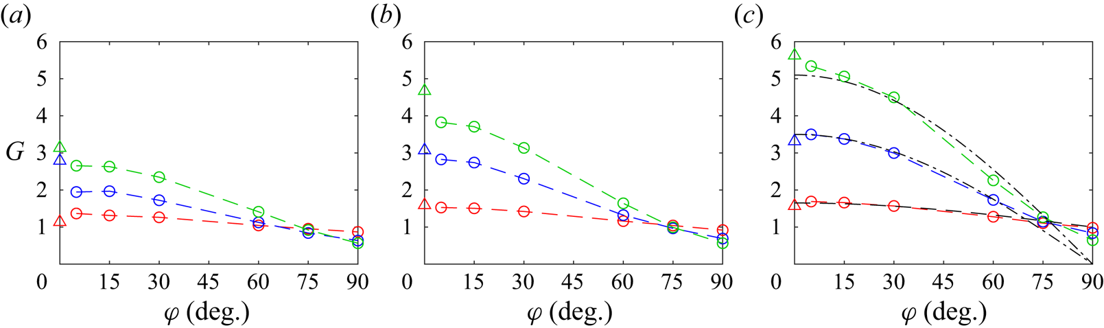
It can be noted that the values of the gains for  $\varphi =5^{\circ }$ are close to, and most often just lower than, those determined for a pulse located on the jet axis in § 3.1, arbitrarily plotted at
 $\varphi =0$ in the figure. This seems consistent with the fact that the pressure waves hitting the nozzle-lip inner corner in the latter case propagate in the upstream direction, with an incidence angle that can be considered as nil, as illustrated in figures 4 and 5. Consequently, the gain in the efficiency of the jet receptivity to acoustic disturbances when the nozzle-lip thickness increases appears to depend mainly on the angle of incidence of the disturbances, whether they be generated in the jet flow or outside.
Finally, the exponents of the power functions (2.2) estimated by curve fitting from the gains  $G$ for the seven pulse positions, inside and outside the jet flow, are shown in figure 17 as a function of the Mach number. For all positions, their values rise with the Mach number as the gains increase faster with the nozzle-lip thickness for a higher jet velocity. More importantly, the values of the exponents are maximum for the pulse position
 $P_{axis}$ and remain significant but slightly decrease between
 $P_{5^{\circ }}$ and
 $P_{30^{\circ }}$. Then they are much lower for
 $P_{60^{\circ }}$, and even become generally negative for
 $P_{75^{\circ }}$ and
 $P_{90^{\circ }}$, as increasing the nozzle-lip thickness reduces the jet receptivity in the two latter cases. Again, these results suggest that the improvement of the efficiency of the scattering of the acoustic disturbances into instability waves for a thicker nozzle lip depends mainly on the angle of incidence of the disturbances, and is progressively stronger when this angle is smaller and tends to zero. Thus the greater improvement is obtained for pressure waves generated in the flow, propagating in the upstream direction with a support both inside and outside the shear layer, i.e. on both sides of the line passing through the nozzle-lip inner corner.
Mach number variations of the exponent  $e$ of the power functions obtained for the gain in receptivity efficiency
 $G$ for an axisymmetric pulse with
 $b=0.2r_0$ located at (black)
 $P_{axis}$, (red)
 $P_{5^{\circ }}$, (blue)
 $P_{15^{\circ }}$, (green)
 $P_{30^{\circ }}$, (yellow)
 $P_{60^{\circ }}$, (cyan)
 $P_{75^{\circ }}$ and (grey)
 $P_{90^{\circ }}$; (circles) simulations and (lines) fitted curves.

3.3. Influence of the azimuthal mode number
The influence of the azimuthal mode number of the acoustic disturbances exciting the jet on the receptivity process is examined from the results provided by the simulations performed for  $M=0.9$ using pulses with
 $n_{\theta }=1$ and 2 located outside the jet at
 $P_{15^{\circ }}$, as mentioned in table 1.
The pressure fluctuations obtained at  $r=r_0$,
 $\theta =0$ and
 $t=t_{z_{WP}}$ using the different nozzle lips for the two azimuthal mode numbers are represented in figures 18(a,b). In the same way as for the axisymmetric pulse in figure 11(b), an instability wave packet is found, peaking at
 $z=z_{WP}=0.75r_0$. In all cases, its amplitude increases when the nozzle lip is thicker. For a given nozzle-lip thickness, it decreases with the azimuthal mode number. For dlip4, for instance, one finds a peak amplitude
 $p'/A=0.97$ for
 $n_{\theta }=0$,
 $p'/A=0.87$ for
 $n_{\theta }=1$, and
 $p'/A=0.62$ for
 $n_{\theta }=2$. The differences between the instability growth rates predicted just downstream of the nozzle lip for
 $n_{\theta }=0$, 1 and 2 using linear stability analysis, shown in figure 2(b), also lead to a reduction of the instability wave amplitudes between
 $z=0$ and
 $z=z_{WP}$ with increasing
 $n_{\theta }$, but to a much lesser degree. This suggests that the jet receptivity to acoustic disturbances is weaker for sound waves with a higher azimuthal mode number.
Pressure fluctuations obtained for  $M=0.9$ at
 $r=r_0$,
 $\theta =0$ and
 $t=t_{z_{WP}}$ for a pulse with
 $b=0.2r_0$ located at
 $P_{15^{\circ }}$, for (a)
 $n_{\theta }=1$ and (b)
 $n_{\theta }=2$, for (black) dlip1, (red) dlip2, (blue) dlip3 and (green) dlip4.

The gains in receptivity efficiency  $G$ obtained with increasing nozzle-lip thickness for the pulses with
 $n_{\theta }=0$, 1 and 2 at
 $P_{15^{\circ }}$ are plotted in figure 19 as a function of
 $\delta _{lip}/r_0$. The three curves are very close to each other, indicating that the improvement of the efficiency of the jet receptivity to the acoustic waves is nearly insensitive to the azimuthal mode number. Thus for resonant jets, especially for screeching and impinging jets, changing the nozzle-lip thickness alone can be expected not to affect the strengths of the resonance mechanisms differently depending on their associated azimuthal modes, and hence not to modify the azimuthal organization of the jets.
Variations with  $\delta _{lip}/r_0$ of the gain in receptivity efficiency
 $G$ obtained for
 $M=0.9$ for pulses located at
 $P_{15^{\circ }}$ with
 $b=0.2r_0$ for (black)
 $n_{\theta }=0$, (red)
 $n_{\theta }=1$ and (blue)
 $n_{\theta }=2$; (circles) simulations and (lines) power functions.

4. Conclusion
In the present study, the variations of the efficiency of the receptivity process of round jets with Blasius laminar (BL) boundary-layer profiles to axisymmetric acoustic waves as functions of the nozzle-lip thickness, the angle of incidence of the waves, and the position where they are generated, inside or outside the flow, have been quantified using numerical simulations for jet Mach numbers between 0.4 and 1.3.
The magnitudes of the Kelvin–Helmholtz instability waves developing in the jet shear layer after the acoustic waves hit the nozzle, hence the jet receptivity efficiency, are shown to increase with the nozzle-lip thickness for guided jet waves travelling upstream in the potential core, and for free-stream sound waves with incidence angles with respect to the jet direction lower than  $75^{\circ }$. The increase is stronger in the first case than in the second, and is weaker when the angle of incidence of the free-stream sound waves is larger. For free-stream sound waves with incidence angles approaching zero, reaching the nozzle-lip final section nearly perpendicularly, however, the gain in efficiency of the jet receptivity is lower but relatively close to that obtained for the guided jet waves. The improvement of the jet receptivity efficiency when a thicker nozzle lip is used is also shown to be greater at a higher Mach number. Moreover, for a Mach number of 0.9, it does not appear to change appreciably when non-axisymmetric azimuthal modes and different spatial extents are considered for the acoustic disturbances, and when the nozzle-exit mean-velocity profile does not correspond to a BL profile.
The consequences of these trends on the feedback loops establishing in jets, notably in impinging and screeching jets, are multiple. Obviously, in line with previous studies in the literature, increasing the nozzle-lip thickness of the jets can be expected to strengthen the feedback loops, which are closed by upstream-propagating guided jet waves or free-stream sound waves in most cases, thus leading to more intense tones in the acoustic field. Given the effects of the incidence angle of the pressure waves and of the position where the waves are generated on the present results, however, thickening the nozzle lip may promote the predominance of the feedback loops closed by guided jet waves over those involving free-stream sound waves, when these two kinds of loops coexist in a jet. Inversely, reducing the nozzle-lip thickness may prevent the establishment of the former feedback loops. Considering the results obtained in this study for different jet velocities, these changes are most likely to be observed at high Mach numbers, in particular for screeching jets in which guided jet waves play the upstream part of the feedback loops producing screech tones. Finally, the simulations performed using non-axisymmetric acoustic disturbances suggest that for resonant jets, a change in the nozzle-lip thickness alone cannot lead to a different azimuthal organization of the jets.
The present results have been obtained for rectangular nozzle lips with sharp corners, and different results could be found for curved nozzle lips and for bevelled corners. In these two cases, the efficiency of the jet receptivity to acoustic disturbances is probably lower than for the nozzle lips in this work. The gain in efficiency as the nozzle-lip thickness increases may also be weaker. This could be investigated in future studies.
Regarding the efficiency of the jet receptivity to free-stream sound waves for a given nozzle-lip thickness, it has been shown to be highest for incidence angles near  $\varphi =90^{\circ }$ for thin nozzle lips, but for angles near
 $\varphi =30^{\circ }$ for thick lips, i.e. when the generation of the shear-layer instability waves mainly involves, respectively, waves reaching the nozzle-lip inner corner and waves reflected by the nozzle-lip final straight section. This could be taken into account when a loudspeaker is placed in the near field of a jet to acoustically excite the shear-layer instability waves downstream of the nozzle and force their development at certain frequencies and azimuthal modes, for flow control or noise reduction purposes, for instance.
Acknowledgements
This work was granted access to the HPC resources of PMCS2I (Pôle de Modélisation et de Calcul en Sciences de l'Ingénieur et de l'Information) of Ecole Centrale de Lyon, and P2CHPD (Pôle de Calcul Hautes Performances Dédiés) of Université Lyon I, and to the resources of IDRIS (Institut du Développement et des Ressources en Informatique Scientifique) and TGCC (Très Grand Centre de calcul du CEA) under the allocation 2023-2a0204 made by GENCI (Grand Equipement National de Calcul Intensif). It was performed within the framework of the LABEX CeLyA (ANR-10-LABX-0060) of Université de Lyon, within the program ‘Investissements d'Avenir’ (ANR-16-IDEX-0005) operated by the French National Research Agency (ANR).
Declaration of interests
The author reports no conflict of interest.
Appendix A. Influence of the pulse half-width
In this appendix, results obtained in the simulations reported in table 3, performed for a jet at  $M=0.9$ with the same boundary-layer profile as the jets in table 1, using acoustic pulses of half-widths
 $b=0.1r_0$ and
 $0.4r_0$ located at
 $P_{axis}$ and
 $P_{30^{\circ }}$, are presented. They are compared with those for the pulse with
 $b=0.2r_0$ provided in §§ 3.1 and 3.2.
Jet boundary layers and Mach numbers, azimuthal mode numbers, half-widths and positions of the acoustic pulses.

The pressure fields calculated for pulses with  $b=0.1r_0$ and
 $0.4r_0$ using dlip3 are shown in figure 20 between
 $t_{d/c_a}$ and
 $t_{d/c_a}+4r_0/u_j$ for the pulse position
 $P_{axis}$, and in figure 21 between
 $t_{d/c_a}$ and
 $t_{d/c_a}+3r_0/u_j$ for
 $P_{30^{\circ }}$. For both positions, the difference in length of the acoustic waves according to the pulse half-width appears clearly, and instability waves develop downstream of the nozzle-lip inner corner after they reach the nozzle. In figures 20(a,b), in particular, the two types of waves moving upstream in the jet potential core for the pulse position
 $P_{axis}$, namely one coming straight from
 $P_{axis}$, the other resulting from the reflection of acoustic waves on the jet shear layer, as discussed in § 3.1, can be seen very distinctly. The second wave is oblique and travels at a velocity close to
 $c_a$, and passes across the first wave propagating at
 $c_a-u_j$ from right to left between the two images.
Pressure fluctuations obtained with dlip3 for  $M=0.9$ for pulses with (a–e)
 $b=0.1r_0$ and ( f–j)
 $b=0.4r_0$ located at
 $\bullet$
 $P_{axis}$ between
 $t=t_{d/c_a}$ and
 $t_{d/c_a}+4r_0/u_j$ in increments of
 $r_0/u_j$, from left to right. The colour scale levels range from
 $-0.06A$ to
 $0.06A$, from blue to red.

Pressure fluctuations obtained with dlip3 for  $M=0.9$ for pulses with (a–d)
 $b=0.1r_0$ and (e–h)
 $b=0.4r_0$ located at
 $\bullet$
 $P_{30^{\circ }}$ between
 $t=t_{d/c_a}$ and
 $t_{d/c_a}+3r_0/u_j$ in increments of
 $r_0/u_j$, from left to right. The colour scale levels range from
 $-0.5A$ to
 $0.5A$, from blue to red.

The pressure fluctuations obtained at  $r=r_0$ and
 $t=t_{z_{WP}}$ for the two pulse positions are represented in figures 22(a,b). The instability wave packets peak at
 $z=z_{WP}=0.9r_0$ for
 $P_{axis}$ and at
 $z=z_{WP}=0.75r_0$ for
 $P_{30^{\circ }}$, in agreement with table 2. In both cases, their amplitudes vary with the pulse half-width, but their shapes do not change much, with one exception. The exception is for the case
 $P_{axis}$ and
 $b=0.4r_0$ in figure 22(a). It can be explained by the presence of acoustic components of significant amplitude at
 $r=r_0$ in this case, as observed in figure 20(h), for example. The dominant wavelength in the wave packet slightly increases with the pulse half-width, but remains close to
 $0.5r_0$. Therefore, the wavelength dominating in the shear layer just downstream of the nozzle lip does not depend much on the pulse half-width. As reported in § 3.1, it corresponds to the wavelength of the most amplified instability waves expected according to linear stability analysis (Bogey Reference Bogey2022a).
Pressure fluctuations obtained with dlip3 for  $M=0.9$ at
 $r=r_0$ and
 $t=t_{z_{WP}}$ for pulses located at (a)
 $P_{axis}$ and (b)
 $P_{30^{\circ }}$, with (black)
 $b=0.1r_0$, (red)
 $b=0.2r_0$ and (blue)
 $b=0.4r_0$.

Finally, the gains in receptivity efficiency  $G$ due to the increase of the nozzle-lip thickness computed for the two pulse positions using (2.1) are plotted as a function of
 $\delta _{lip}/r_0$ in figures 23(a,b). For both positions, the values of the gains are very similar for the three pulse half-widths. This suggests that the results obtained in this study regarding the improvement of the jet receptivity as a thicker nozzle lip is used do not depend on the half-width of the pulses introduced in the simulations.
Variations with  $\delta _{lip}/r_0$ of the gain in receptivity efficiency
 $G$ obtained for
 $M=0.9$ for pulses located at (a)
 $P_{axis}$ and (b)
 $P_{30^{\circ }}$, with (black)
 $b=0.1r_0$, (red)
 $b=0.2r_0$ and (blue)
 $b=0.4r_0$; (circles) simulations and (lines) power functions.

Appendix B. Influence of the boundary-layer profile
In this appendix, two jets at  $M=0.9$ with boundary-layer velocity profiles different from the BL profile are considered. The profiles correspond to the transitional boundary-layer profiles T1 and T2 with shape factors
 $H=1.88$ and
 $1.52$ defined in Bogey & Sabatini (Reference Bogey and Sabatini2019), displayed in figure 24(a). They have the same momentum thickness
 $\delta _{\theta }=0.012 r_0$ as the BL profile used in all other simulations. An axisymmetric acoustic pulse of half-width
 $b=0.2r_0$ located at
 $P_{30^{\circ }}$ is introduced in the two cases, as documented in table 4.
Representation of (a) the axial velocity  $u_z/u_j$ and (b) the variations with
 $\delta _{lip}/r_0$ of the gain in receptivity efficiency
 $G$ obtained for
 $M=0.9$ for an axisymmetric pulse at
 $P_{30^{\circ }}$ with
 $b=0.2r_0$, using the (black) BL, (red) T1 and (blue) T2 profiles; (circles) simulations and (lines) power functions.

Jet boundary layers and Mach numbers, azimuthal mode numbers, half-widths and positions of the acoustic pulses.

The gains in receptivity efficiency  $G$ obtained when the nozzle lip is thicker from the instability wave amplitudes at
 $t=t_{z_{WP}}$ for the boundary-layer profiles BL, T1 and T2 are plotted in figure 24(b) as a function of
 $\delta _{lip}/r_0$. They are quite similar in the three cases. Therefore, they seem little sensitive to the shape of the nozzle-exit mean-velocity profiles. Obviously, in real jets with transitional or turbulent boundary layers, velocity disturbances of high amplitude are found in the nozzle-exit section, which is not the case in the present simulations. They can be expected to alter the jet receptivity to external acoustic waves, which would be interesting to investigate in future studies.


 Open access

