



1. Introduction
1.1. Setting
Since the early 1990s, stochastic differential equations (SDEs) with Markovian switching have attracted considerable interest. These models comprise two key components: (i) a continuous-time dynamical system that follows one of finitely many underlying Markovian dynamics, with transitions dictated by (ii) an underlying continuous-time Markov chain. Such random switching processes find broad applications in fields like financial engineering, risk management, and operations research [Reference Bardet, Guérin and Malrieu3, Reference Cloez and Hairer8, Reference Ji and Chizeck12, Reference Kunwai and Zhu18, Reference Mao and Yuan23, Reference Shao30, Reference Shao31, Reference Xi36, Reference Xi37, Reference Xi and Zhu38, Reference Yin and Zhu39, Reference Zong, Wu, Yin and Jin41].
We study the following stable SDE with Markovian switching: the first component
 $(X_t)_{t\geqslant 0}$
satisfies
 \begin{equation} \mathrm{d}X_t = g(X_t,R_t)\,\mathrm{d}t + \sigma\,\mathrm{d}Z_t, \quad (X_0,R_0) \in \mathbb{R}^d\times\mathbb{S},\end{equation}
where
 $(Z_t)_{t\geqslant 0}$
is a d-dimensional rotationally invariant
 $\alpha$
-stable process with
 $\alpha \in (1,2)$
and
 $\sigma$
is a nondegenerate constant matrix, the switching part
 $(R_t)_{t\geqslant 0}$
is a continuous-time Markov chain with a finite state space
 $\mathbb{S}=\{1,2,\ldots,N\}$
and an irreducible transition rate matrix
 $Q=(q_{ij})_{1\leqslant i,j \leqslant N}$
. The entries of Q satisfy
 $q_{ij} \geqslant 0$
for all
 $i\neq j$
and
 $q_{ii}=-\sum_{j\neq i} q_{ij}$
for all
 $i\in \mathbb{S}$
, and the transition probability for
 $(R_t)_{t\geqslant 0}$
is given by
 $\mathrm{e}^{Qt}$
[Reference Mao and Yuan23, Theorem 1.44], which implies that, for any
 $u,v \in \mathbb{S}$
,
 \begin{align*} \mathbb{P}(R_{t+\Delta}=v \mid R_t=u) = \left\{\begin{array}{ll} q_{uv}\Delta + o(\Delta) &\quad \text{if } v \neq u, \\[3pt] 1+q_{uv}\Delta + o(\Delta) &\quad \text{if } v=u \end{array} \right.\end{align*}
for some small enough
 $\Delta>0$
, where
 $a=o(\Delta)$
means
 $\lim_{\Delta \to 0} {a}/{\Delta}=0$
.
We impose the following assumptions on the coefficient g in SDE (1.1).
Assumption 1.1.
-
(i) There exist
 $\{c_i,i \in \mathbb{S}\}$
with
$c_i \in \mathbb{R}$
such that, for all
$x,y\in \mathbb{R}^d$
and
$i\in \mathbb{S}$
, (1.2)
\begin{equation} \langle x, \nabla g(y,i)x \rangle \leqslant c_i |x|^2. \end{equation}
-
(ii) For
$i\in \mathbb{S}$
,
$g(\cdot,i)\in \mathcal{C}^2(\mathbb{R}^d,\mathbb{R}^d)$
and
$\nabla^m g(\cdot,i)$
(
$m=0,1,2$
) are Lipschitz continuous.





Under Assumption 1.1, the system in (1.1) admits a unique strong solution
 $(X_t,R_t)_{t\geqslant 0}$
for any initial value
 $(X_0,R_0)\in \mathbb{R}^d \times \mathbb{S}$
(see [Reference Mao and Yuan23] and [Reference Xi and Zhu38, Theorem 2.1]). Conditioned on
 $R_t=i$
, the first component, denoted by
 $X_t^{(i)}$
, follows
 $\mathrm{d}X_t^{(i)} = g(X_t^{(i)}, i)\,\mathrm{d}t + \sigma\,\mathrm{d}Z_t$
. Crucially, the constants
 $\{c_{\ell},\ell\in \mathbb{S}\}$
take values in
 $\mathbb{R}$
, rather than
 $(\! -\infty,0)$
; this is a pivotal condition for the coefficient g: for some switching state
 $i\in \mathbb{S}$
with
 $c_i>0$
, the corresponding
 $X_t^{(i)}$
may exhibit explosive behavior as
 $t \to \infty$
, but the switching component
 $(R_t)_{t\geqslant 0}$
can transition to a state
 $j\neq i$
with
 $c_j<0$
, which acts to stabilize the process
 $(X_t)_{t\geqslant 0}$
. Thus, the switching component
 $(R_t)_{t\geqslant 0}$
regulates the dynamics by alternating between different stable SDEs
 $(X_t^{(i)})_{t\geqslant 0}$
with
 $i\in \mathbb{S}$
.
To approximate the law of the process
 $(X_t,R_t)_{t\geqslant 0}$
in SDE (1.1), we construct an Euler–Maruyama (EM) scheme with step size
 $\gamma$
. For
 $(Y_0,R_0)=(X_0,R_0)$
and
 $n\in \mathbb{N}_0=\mathbb{N}_+ \cup \{0\}$
with
 $\mathbb{N}_+=\{1,2,\ldots\}$
, the EM scheme reads
 $Y_{t_{n+1}} = Y_{t_n} + \gamma g(Y_{t_n},R_{t_n})+\sigma\Delta Z_{\gamma}$
, where
 $t_n=n\gamma$
,
 $\Delta Z_{\gamma}=Z_{t_{n+1}}-Z_{t_n}$
, and
 $(R_{t_n})_{n\in \mathbb{N}_0}$
is a Markov chain with one-step transition probability matrix
 $\mathrm{e}^{\gamma Q}$
.
1.2. Related works
Since the transition rate matrix Q is constant, the switching process
 $(R_t)_{\geqslant 0}$
is a continuous-time Markov chain that is independent of the rotationally invariant
 $\alpha$
-stable process
 $(Z_t)_{t\geqslant 0}$
. For more details about SDEs with Markovian switching, we refer the reader to [Reference Mao and Yuan23, Reference Yin and Zhu39]. Extensive research has established fundamental results on the stability, ergodicity, and asymptotic behavior of such processes [Reference Bao, Shao and Yuan2, Reference Cloez and Hairer8, Reference Kunwai and Zhu18, Reference Li and Xi19, Reference Mao22, Reference Nguyen, Yin and Zhu27, Reference Shao30, Reference Shao31, Reference Xi35–Reference Xi and Zhu38, Reference Yuan and Mao40, Reference Zong, Wu, Yin and Jin41].
Recent studies have made significant progress in analyzing regime-switching processes through various approaches. [Reference Kunwai and Zhu18, Reference Xi and Zhu38] employed coupling techniques and Radon–Nikodym derivatives to investigate both Feller and strong Feller properties along with exponential ergodicity for regime-switching jump processes with countable state spaces. Based on the strong Feller property and irreducibility, [Reference Cloez and Hairer8, Reference Li and Xi19, Reference Shao30] developed verifiable criteria for the ergodicity of random switching processes driven by Brownian motion or pure jump processes. Stability properties were thoroughly examined in [Reference Ji and Chizeck12, Reference Mao22, Reference Mao and Yuan23, Reference Yin and Zhu39], while asymptotic behavior was considered in [Reference Bardet, Guérin and Malrieu3, Reference Xi36, Reference Xi37, Reference Yin and Zhu39]. [Reference Xi35] used the Radon–Nikodym derivative and constructed an auxiliary process to derive fundamental properties, including Feller and strong Feller properties and ergodicity, for state-dependent switching diffusion processes.
1.2.1. EM scheme for SDEs with regime switching.
Closed-form expressions for the laws or ergodic measures of SDEs are generally unavailable, with notable exceptions including one-dimensional diffusions [Reference Klebaner16, p. 171] and Langevin SDEs [Reference Fang, Shao and Xu10, p. 555]. The EM scheme provides a practical approximation for these measures. Recent advances include the following: [Reference Fang, Shao and Xu10] used Malliavin calculus and Stein’s equation to investigate the Wasserstein-1 distance for diffusions and their constant step-size EM schemes; [Reference Bras, Pagés and Panloup4, Reference Pagès and Panloup28] applied Malliavin calculus and the Lindeberg principle to discuss the Wasserstein-1 and total variation distances for diffusions and their various step-size EM schemes; and [Reference Chen, Deng, Schilling and Xu5, Reference Chen, Jin, Xiao and Xu7] were concerned with constant and variable step-size EM schemes for stable SDEs and obtained the convergence rate in Wasserstein-1 distance. Additionally, strong convergence properties were established in [Reference Liu and Mao20, Reference Shao31, Reference Yuan and Mao40].
While explicit solutions for SDEs with Markovian switching remain elusive, the EM scheme provides an effective approximation tool. Previous studies [Reference Bao, Shao and Yuan2, Reference Shao31, Reference Yin and Zhu39, Reference Yuan and Mao40] established convergence results for random switching diffusions using the EM scheme. Recently, [Reference Chen, Jin, Shen and Su6, Reference Jin, Shen and Su14] used constant and decreasing step-size EM schemes to approximate the law for regime-switching jump processes, though limited to dissipative drift conditions and excluding rotationally invariant
 $\alpha$
-stable processes. This paper extends their framework to SDEs driven by d-dimensional rotationally invariant
 $\alpha$
-stable processes (
 $\alpha \in (1,2)$
), analyzing both the EM approximation and its asymptotic properties.
1.2.2. Central limit theorem and moderate deviation principle for empirical measures.
Propositions A.1 and A.2 establish exponential ergodicities for both the original process
 $(X_t,R_t)_{t\geqslant 0}$
and its EM scheme
 $(Y_{t_n},R_{t_n})_{n\in \mathbb{N}_0}$
with ergodic measures
 $\mu$
and
 $\mu_{\gamma}$
respectively. By the Birkhoff ergodic theorem, the empirical measures
 $\mathcal{E}_T^{(x,k)}$
and
 $\mathcal{E}_{n,\gamma}^{(x,k)}$
(definitions in (2.1) and (2.2) respectively) converge almost surely to
 $\mu$
and
 $\mu_{\gamma}$
, i.e.
 $\lim_{T\to \infty} \mathcal{E}_T^{(x,k)} = \mu$
and
 $\lim_{n\to \infty} \mathcal{E}_{n,\gamma}^{(x,k)} = \mu_{\gamma}$
almost surely, as shown in [Reference Da and Zabczyk9]. For diffusion processes, prior work has investigated limit theorems for empirical measures: [Reference Jin, Pang, Xu and Xu13] derived central limit theorems (CLTs) and moderate deviation principles (MDPs) for both the diffusion and its EM scheme, while [Reference Lu, Tan and Xu21] established the CLT and Cramér-type moderate deviation for the EM approximation. In the case of
 $\alpha\in (1,2)$
, it is natural to investigate whether analogous CLT and MDP results hold for the regime-switching process
 $(X_t,R_t)_{t\geqslant 0}$
and its EM scheme
 $(Y_{t_n},R_{t_n})_{n\in \mathbb{N}_0}$
.
1.3. Preliminaries
For any given real number
 $\kappa$
, define the matrix
 $Q_{c,\kappa}$
as
 \begin{align} Q_{c,\kappa} = Q + \kappa\operatorname{diag}(c_1,\ldots,c_N), \end{align}
where
 $\operatorname{diag}(c_1,\ldots,c_N)$
is the diagonal matrix formed by the vector
 $(c_1,\ldots,c_N)$
, and the constants
 $c_1,\ldots,c_N$
are defined in (1.2).
Assumption 1.2. There exist two constants
 $\kappa_1 \in (1,\alpha)$
and
 $\kappa_2\in (0,\kappa_1/4]$
such that the matrices
 $-Q_{c,\kappa_1}$
and
 $-Q_{c,\kappa_2}$
are both nonsingular M-matrices.
It follows from [Reference Shao31, Lemma 2.1] or [Reference Bardet, Guérin and Malrieu3, Proposition 4.1] that the following lemma holds.
Lemma 1.1. Under Assumptions 1.1 and 1.2, and for the matrix
 $Q_{c,4}$
defined in (1.3), let
 \begin{equation} \eta = -\max_{\theta\in\operatorname{spec}(Q_{c,4})}\operatorname{Re}(\theta), \end{equation}
where
 $\operatorname{spec}(Q_{c,4})$
denotes the spectrum of matrix
 $Q_{c,4}$
, and
 $\operatorname{Re}(\theta)$
is the real part of
 $\theta$
. Assume that
 $\eta>0$
. Then, for
 $\{c_{\ell}, \ell \in \mathbb{S} \}$
in (1.2), there exists some constant
 $C>0$
such that
 \begin{equation*} \mathbb{E}\exp\bigg(4\int_0^t c_{R_s}\,\mathrm{d}s\bigg) \leqslant C\mathrm{e}^{-\eta t} \quad \textit{for all } t\geqslant 0. \end{equation*}
Remark 1.1. The parameter
 $\kappa_1$
in Assumption 1.2 is crucial for obtaining the convergence rate of the EM approximation (see more details in Theorem 2.1) and for the moment estimates (see Lemma 3.2). Assume that
 $\eta>0$
. Lemma 1.1 plays an important role in estimating Jacobi flows for the process
 $(X_t,R_t)_{t\geqslant 0}$
(see Lemma C.1 for further details).
1.4. Notation
Denote by
 $(X_t^{x,k},R_t^{k})$
the solution to the system (1.1) with initial value
 $(X_0,R_0)=(x,k)$
, and define its semigroup
 $P_{t}$
by
 $P_{t} \, f(x,k)=\mathbb{E} f(X_t^{x,k},R_t^{k})$
for any bounded Borel function
 $f\in \mathcal{B}_\mathrm{b}(\mathbb{R}^d\times \mathbb{S},\mathbb{R})$
and
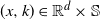 $(x,k)\in \mathbb{R}^d\times \mathbb{S}$
. For the EM scheme
 $(Y_{t_n}^{x,k},R_{t_n}^{k})$
initialized at
 $(Y_0,R_0)=(x,k)$
, let
 $\bar{P}_{\gamma}$
be its transition semigroup
 $\bar{P}_{\gamma}f(x,k)= \mathbb{E} f(Y_{\gamma}^{x,k},R_{\gamma}^k)$
, with
 $\bar{P}_{\gamma}^m=\bar{P}_{\gamma} \circ \bar{P}_{\gamma}^{m-1}$
for integers
 $m\geqslant 2$
.
Let M be a matrix, and denote its transpose by
 $M^*$
. We write
 $M\geqslant 0$
if all entries of M are nonnegative, and
 $M\gg 0$
if all entries are strictly positive. For a vector M,
 $M_i$
represents its ith component. The Hilbert–Schmidt norm of an
 $\mathbb{R}^{d\times d}$
matrix
 $M=(M_{ij})_{d\times d}$
is given by
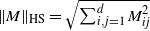 $\| M \|_\textrm{HS}=\sqrt{\sum_{i,j=1}^d M_{ij}^2}$
.
Since the state space for the process
 $(X_t,R_t)_{t\geqslant 0}$
is
 $\mathbb{R}^d \times \mathbb{S}$
, and for
 $f(\cdot,\cdot) \in \mathcal{C}^m(\mathbb{R}^d \times \mathbb{S})$
with integers
 $m\geqslant 1$
,
 $\nabla^m f(x,k)$
refers to the mth-order partial derivative with respective to x (with k fixed), and
 $\nabla_u f$
represents the directional derivative along the direction
 $u\in \mathbb{R}^d$
. For
 $f\in \mathcal{C}^2(\mathbb{R}^d \times \mathbb{S},\mathbb{R})$
, define
 \begin{align*} \|\nabla^i f\|_{\infty} & = \sup_{k\in\mathbb{S}}\|\nabla^i f(\cdot,k)\|_{\infty} = \sup_{(x,k)\in\mathbb{R}^d\times\mathbb{S}}|\nabla^i f(x,k)|, \quad i=0,1; \nonumber \\[2pt] \|\nabla^2 f\|_{\infty} & = \sup_{k\in\mathbb{S}}\|\nabla^2 f(\cdot,k)\|_\textrm{HS} = \sup_{(x,k)\in\mathbb{R}^d\times\mathbb{S}}\|\nabla^2 f(x,k)\|_\textrm{HS}.\end{align*}
For a
 $\tau$
-Hölder continuous function f defined on A with
 $\tau\in (0,1]$
, define
 \begin{align*}[f]_{\tau;A} = \sup_{x,y\in A, x\neq y}\frac{|f(x)-f(y)|}{|x-y|^{\tau}}. \end{align*}
Let
 $\mathcal{G}=\{h\in\mathcal{C}^2(\mathbb{R}^d\times\mathbb{S},\mathbb{R})\colon\|\nabla^i h\|_{\infty}<\infty$
with
 $i=1,2\}$
. We introduce a metric
 $\operatorname{dist}(\cdot,\cdot)$
on
 $\mathbb{R}^d \times \mathbb{S}$
as follows (see [Reference Yin and Zhu39, (9.6)] or [Reference Shao31, p. 3229]):
 \begin{align*} \operatorname{dist}((x,i),(y,j))=|x-y|+d(i,j), \qquad \text{where } d(i,j) = \left\{ \begin{array}{ll} 1 &\quad \text{if } j\neq i, \\[2pt] 0 &\quad \text{if } j = i. \end{array} \right.\end{align*}
Let
 $\mathcal{B}(\mathbb{R}^d \times \mathbb{S})$
be the collection of Borel sets on
 $\mathbb{R}^d \times \mathbb{S}$
, and
 $\mathcal P$
denote the space of probability measures on
 $(\mathbb{R}^d\times \mathbb{S},\mathcal{B}(\mathbb{R}^d\times \mathbb{S}))$
; define
 \begin{equation*} \mathcal P_0 = \bigg\{\mu_1\in\mathcal P\colon\mu_1(h) = \int_{\mathbb{R}^d\times\mathbb{S}}h(x,k)\,\mathrm{d}\mu_1(x,k) < \infty \text{ for any } h\in\mathcal G\bigg\}.\end{equation*}
For
 $\mu_1, \mu_2\in\mathcal P_0$
, we define the distance
 $d_{\mathcal{G}}(\mu_1,\mu_2)$
as
 \begin{equation} d_{\mathcal{G}}(\mu_1,\mu_2) = \sup_{h\in\mathcal{G}}\bigg\{ \int_{\mathbb{R}^d\times\mathbb{S}}h(x,k)\,\mathrm{d}\mu_1(x,k) - \int_{\mathbb{R}^d\times\mathbb{S}}h(x,k)\,\mathrm{d}\mu_2(x,k)\bigg\}.\end{equation}
Clearly,
 $d_{\mathcal{G}}(\cdot,\cdot)$
is a metric on
 $\mathcal P_0$
. For any random vector X, denote its law by
 $\mathcal{L}(X)$
.
A sequence of random variables
 $\{Y_n, n\geqslant 1 \}$
is said to converge weakly (or converge in distribution) to a limit
 $Y_{\infty}$
; we write
 $Y_n \Rightarrow Y_{\infty}$
if
 $\lim_{n \rightarrow \infty} \mathbb{E} f(Y_{n})=\mathbb{E} f(Y_{\infty})$
for all bounded continuous functions f. Additionally,
 $Y_n \stackrel{\mathrm{p}}{\longrightarrow} Y_{\infty}$
means convergence in probability, namely,
 $\lim_{n\to \infty} \mathbb{P}(|Y_n - Y_{\infty}|>\delta)=0$
for all
 $\delta > 0$
.
For a given probability measure
 $\nu$
, define
 $L^2(\nu)$
as the Hilbert space induced by
 $\nu$
with inner product
 $\langle f_1, f_2\rangle_{\nu} = \int f_1 f_2\,\mathrm{d}\nu \textrm{ for } f_1,f_2 \in L^2(\nu)$
.
1.5. Strategy
We conclude this section by outlining the proof strategy for our main results. The main results presented in Section 2 include the EM approximation, CLT, and MDP for empirical measures of an SDE and its EM scheme, with detailed proofs provided in Sections 3, 4, and 5 respectively. Our approach involves approximating the law of the process
 $(X_t,R_t)_{t\geqslant 0}$
by its EM scheme
 $(Y_{t_n},R_{t_n})_{n\in \mathbb{N}_0}$
, and establishing the convergence rate under the metric
 $d_{\mathcal{G}}$
, as shown in Theorem 2.1. Applying the Lindeberg principle from [Reference Pagès and Panloup28], we know that
 \begin{align*} d_{\mathcal{G}}\big(\mathcal{L}\big(X_{t_n}^{x,k},R_{t_n}^{k}\big), \mathcal{L}\big(Y_{t_n}^{x,k},R_{t_n}^{k}\big)\big) & = \sup_{h\in\mathcal{G}}\{P_{t_n}h(x,k) - \bar{P}_{t_n}h(x,k)\} \nonumber \\[2pt] & = \sup_{h\in\mathcal{G}}\Bigg\{\sum_{i=1}^{n}\bar{P}_{t_{i-1}} \circ (P_{\gamma}-\bar{P}_{\gamma}) \circ P_{t_n-t_i}h(x,k)\Bigg\}.\end{align*}
The term
 $(P_{\gamma}-\bar{P}_{\gamma})f(x,k)$
with
 $f(x,k)=P_{t_n-t_i} h(x,k)$
plays a crucial role in estimating
 $d_{\mathcal{G}}\big(\mathcal{L}\big(X_{t_n}^{x,k},R_{t_n}^{k}\big),\mathcal{L}\big(Y_{t_n}^{x,k},R_{t_n}^{k}\big)\big)$
. We refer to this term as the one-step difference between the process
 $(X_t,R_t)_{t\geqslant 0}$
and its EM scheme
 $(Y_{t_n},R_{t_n})_{n\in \mathbb{N}_0}$
; this is given in Lemma 3.3, whose proof is provided in Appendix B. After estimating the one-step difference, gradient estimates for the semigroup
 $P_{t}$
are also essential (see Lemma 3.1), and their proofs can be found in Appendix C. Additionally, moment estimates for the process
 $(X_t,R_t)_{t\geqslant 0}$
and its EM scheme
 $(Y_{t_n},R_{t_n})_{n\in \mathbb{N}_0}$
are given in Lemma 3.2 with proofs in Appendix A, obtained by the Lyapunov condition and the generator comparison. Finally, we employ various types of Stein’s equations to prove the CLT and MDP for empirical measures of the SDE and its EM scheme.
2. Main results and an example
2.1. Main results
Our first main result concerns the EM approximation, which quantifies the error between the laws of the SDE
 $(X_t,R_t)_{t\geqslant 0}$
and its EM scheme
 $(Y_{t_n},R_{t_n})_{n\in \mathbb{N}_0}$
; the proof is provided in Section 3.
Theorem 2.1. Under Assumptions 1.1 and 1.2, with
 $\eta>0$
defined in (1.4), there exists some positive constant C, independent of
 $\gamma$
, x, k, and
 $t_n$
, such that
 \begin{equation*} d_{\mathcal{G}}\big(\mathcal{L}\big(X_{t_n}^{x,k},R_{t_n}^{k}\big),\mathcal{L}\big(Y_{t_n}^{x,k},R_{t_n}^{k}\big)\big) \leqslant C(1+|x|^{\kappa_1})\gamma^{{\kappa_1}/{\alpha}}, \end{equation*}
where the distance
 $d_{\mathcal{G}}$
is defined in (1.5), and the constant
 $\kappa_1$
is from Assumption 1.2.
Remark 2.1. When the state space
 $\mathbb{S}=\{1\}$
and
 $c_1<0$
with
 $c_1$
defined in (1.2), we know that Assumption 1.2 holds for any
 $\kappa_1 \in (1,\alpha)$
. In this case, the process
 $(X_t,R_t)_{t\geqslant 0}$
reduces to a stable SDE
 $(X_t)_{t\geqslant 0}$
without Markovian switching. The convergence rate for the EM scheme aligns precisely with those in [Reference Chen, Deng, Schilling and Xu5, Theorem 1.3] and [Reference Chen, Jin, Xiao and Xu7, Theorem 1.9].
Our second set of main results establishes the CLT and MDP for the long-term behavior of the process
 $(X_t,R_t)_{t\geqslant 0}$
and its EM scheme
 $(Y_{t_n},R_{t_n})_{n\in \mathbb{N}_0}$
; proofs of these results can be found in Sections 4 and 5 respectively.
For any
 $(x,k)\in \mathbb{R}^d\times \mathbb{S}$
and
 $T>0$
, the empirical measure
 $\mathcal{E}_T^{(x,k)}$
of the process
 $(X_t,R_t)_{t\geqslant 0}$
is defined by
 \begin{equation} \mathcal{E}_T^{(x,k)}(A) = \frac{1}{T}\int_0^T\delta_{(X_s^{x,k},R_s^k)}(A)\,\mathrm{d}s, \quad A \in \mathcal{B}(\mathbb{R}^d\times \mathbb{S}),\end{equation}
where
 $\delta_{y}(\! \cdot \!)$
is the Dirac delta measure defined as
 $\delta_{y}(A)=1$
if
 $y\in A$
and
 $\delta_{y}(A)=0$
otherwise. It is straightforward to verify that, for any continuously differentiable bounded Borel-measurable function
 $h\in \mathcal{C}^1_\mathrm{b}(\mathbb{R}^d\times \mathbb{S},\mathbb{R})$
,
 $\mathcal{E}_T^{(x,k)}(h) = ({1}/{T})\int_0^T h(X_s^{x,k},R_s^k)\,\mathrm{d}s$
.
For any
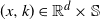 $(x,k)\in \mathbb{R}^d\times \mathbb{S}$
and
 $n\in \mathbb{N}_+$
, the empirical measure
 $\mathcal{E}_{n,\gamma}^{(x,k)}$
of the EM scheme
 $(Y_{t_n},R_{t_n})_{n\in \mathbb{N}_0}$
is defined by
 \begin{equation} \mathcal{E}_{n,\gamma}^{(x,k)}(A) = \frac{1}{n}\sum_{i=0}^{n-1}\delta_{(Y_{t_i}^{x,k},R_{t_i}^k)}(A), \quad A \in \mathcal{B}(\mathbb{R}^d\times \mathbb{S}).\end{equation}
It is easy to verify that, for any
 $h\in\mathcal{C}^1_\mathrm{b}(\mathbb{R}^d\times\mathbb{S},\mathbb{R})$
,
 $\mathcal{E}_{n,\gamma}^{(x,k)}(h) = ({1}/{n})\sum_{i=0}^{n-1}h\big(Y_{t_i}^{x,k},R_{t_i}^k\big)$
.
Theorem 2.2. (Central limit theorem.) Under Assumptions 1.1 and 1.2, with
 $\eta>0$
defined in (1.4), for
 $h\in\mathcal{C}_\mathrm{b}^1(\mathbb{R}^d\times\mathbb{S},\mathbb{R})$
and
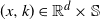 $(x,k)\in\mathbb{R}^d\times\mathbb{S}$
, the term
 $\sqrt{t}\big[\mathcal{E}_t^{(x,k)}(h)-\mu(h)\big]$
converges weakly to the Gaussian distribution
 $\mathcal{N}(0,\mathcal{V}(f_h))$
as
 $t\to\infty$
, where
 $\mathcal{V}(f_h)$
is given by
 \begin{align} \mathcal{V}(f_h) & = \int_{\mathbb{R}^d\times\mathbb{S}}\int_{\mathbb{R}_0^d}|f_h(x+\sigma z,k)-f_h(x,k)|^2\,\nu(\mathrm{d}z)\, \mathrm{d}\mu(x,k) \nonumber \\[3pt] & \quad + \int_{\mathbb{R}^d\times\mathbb{S}}\int_{\mathbb{R}_0}|f_h(x,k+\ell(k,\tilde{z}))-f_h(x,k)|^2\, \mathrm{d}\tilde{z}\,\mathrm{d}\mu(x,k), \end{align}
where
 $\mu$
is the ergodic measure for the process
 $(X_t,R_t)_{t\geqslant 0}$
,
 $f_h$
is the solution to Stein’s equation (4.5),
 $\ell$
is defined in (4.1), and
 $\nu$
is the Lévy measure in (4.2).
Theorem 2.3. (Moderate deviation principle.) Under Assumptions 1.1 and 1.2, with
 $\eta>0$
defined in (1.4), for any
 $h\in\mathcal{C}_\mathrm{b}^1(\mathbb{R}^d\times\mathbb{S},\mathbb{R})$
,
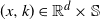 $(x,k)\in\mathbb{R}^d\times\mathbb{S}$
, and any measurable set
 $A\subseteq \mathbb{R}$
, we have
 \begin{align*} -\inf_{z\in\it{\unicode{x00C5}}}\frac{z^2}{2\mathcal{V}(f_h)} & \leqslant \liminf_{t\to\infty}\frac{1}{a_t^2}\log\mathbb{P}\bigg( \frac{\sqrt{t}}{a_t}\big[\mathcal{E}_t^{(x,k)}(h)-\mu(h)\big]\in A\bigg) \nonumber \\[3pt] & \leqslant \limsup_{t\to\infty}\frac{1}{a_t^2}\log\mathbb{P}\bigg( \frac{\sqrt{t}}{a_t}\big[\mathcal{E}_t^{(x,k)}(h)-\mu(h)\big]\in A\bigg) \leqslant -\inf_{z\in\bar{A}}\frac{z^2}{2\mathcal{V}(f_h)}, \end{align*}
where
 $\mu$
is the ergodic measure for the process
 $(X_t,R_t)_{t\geqslant 0}$
, sets
 $\bar{A}$
and
 $\it{\unicode{x00C5}}$
denote the closure and interior of A respectively, the function
 $a_t$
satisfies
 $a_t\to \infty$
and
 $t^{-1/2}a_t\to 0$
as
 $t\to \infty$
, and
 $\mathcal{V}(f_h)$
is defined in (2.3).
Theorem 2.4. (CLT and MDP.) Under Assumptions 1.1 and 1.2, with
 $\eta>0$
defined in (1.4), let
 $\mu_{\gamma}$
be the ergodic measure for the EM scheme
 $(Y_{t_n},R_{t_n})_{n\in \mathbb{N}_0}$
. For
 $h\in\mathcal{C}_\mathrm{b}^1(\mathbb{R}^d\times\mathbb{S},\mathbb{R})$
and
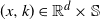 $(x,k)\in\mathbb{R}^d\times\mathbb{S}$
,
-
(i) The term
$\sqrt{n}\big[\mathcal{E}_{n,\gamma}^{(x,k)}(h)-\mu_{\gamma}(h)\big]$
converges weakly to the Gaussian distribution
$\mathcal{N}(0$
,
$\widetilde{\mathcal{V}}(f_{\gamma,h}))$
as
$n\to\infty$
, where
$\widetilde{\mathcal{V}}(f_{\gamma,h})$
is given by (2.4)with
\begin{equation} \widetilde{\mathcal{V}}(f_{\gamma,h}) = \langle f_{\gamma,h},f_{\gamma,h}\rangle_{\mu_{\gamma}} - \langle\bar{P}_{\gamma}f_{\gamma,h},\bar{P}_{\gamma}f_{\gamma,h}\rangle_{\mu_{\gamma}}, \end{equation}
$f_{\gamma,h}$
the solution to Stein’s equation (5.1). Moreover, the term
$\widetilde{\mathcal{V}}(f_{\gamma,h})$
can also be expressed as
\begin{equation*} \widetilde{\mathcal{V}}(f_{\gamma,h}) = \langle h-\mu_{\gamma}(h),h-\mu_{\gamma}(h)\rangle_{\mu_{\gamma}} + \sum_{i=1}^{\infty}\langle\bar{P}_{\gamma}^i h,h-\mu_{\gamma}(h)\rangle_{\mu_{\gamma}}. \end{equation*}
-
(ii) For any measurable set
$A\subseteq \mathbb{R}$
, we know that where
\begin{align*} -\inf_{z\in\it{\unicode{x00C5}}}\frac{z^2}{2\widetilde{\mathcal{V}}(f_{\gamma,h})} & \leqslant \liminf_{n\to\infty}\frac{1}{a_n^2}\log\mathbb{P}\bigg( \frac{\sqrt{n}}{a_n}\big[\mathcal{E}_{n,\gamma}^{(x,k)}(h)-\mu_{\gamma}(h)\big]\in A\bigg) \\[2pt] & \leqslant \limsup_{n\to\infty}\frac{1}{a_n^2}\log\mathbb{P}\bigg( \frac{\sqrt{n}}{a_n}\big[\mathcal{E}_{n,\gamma}^{(x,k)}(h)-\mu_{\gamma}(h)\big]\in A\bigg) \leqslant -\inf_{z\in\bar{A}}\frac{z^2}{2\widetilde{\mathcal{V}}(f_{\gamma,h})}, \end{align*}
$\bar{A}$
and
$\it{\unicode{x00C5}}$
are the closure and interior of the set A respectively, the function
$a_n$
satisfies
$a_n\to\infty$
and
$n^{-1/2}a_n\to 0$
as
$n\to\infty$
, and
$\widetilde{\mathcal{V}}(f_{\gamma,h})$
is defined in (2.4).



2.2. An example
We begin by recalling several equivalent characterizations of nonsingular M-matrices; detailed treatments can be found in [Reference Shao30, Proposition 2.4] and [Reference Mao22, Lemma 4.2].
Lemma 2.1. The following statements are equivalent:
-
(i) The matrix A is a nonsingular
$d\times d$
M-matrix. -
(ii) All of the principal minors of matrix A are positive, i.e.
\begin{align*} \begin{vmatrix} a_{11} &\quad \cdots &\quad a_{1i} \\[2pt] \vdots &\quad \ddots &\quad \vdots \\[2pt] a_{i1} &\quad \cdots &\quad a_{ii} \end{vmatrix} > 0 \quad \text{for every } i= 1,2,\ldots,d. \end{align*}
-
(iii) Every real eigenvalue of matrix A is positive.
-
(iv) The matrix A is semi-positive, i.e. there exists a vector
$x\gg 0$
such that
$Ax \gg 0$
.


Example 2.1. We consider a one-dimensional SDE driven by the rotationally invariant
 $\alpha$
-stable process
 $(\alpha \in (1,2))$
with Markovian switching:
 \begin{align} \mathrm{d}X_t = g(X_t,R_t)\,\mathrm{d}t + \mathrm{d}Z_t, \quad (X_0,R_0)\in\mathbb{R}\times\mathbb{S}, \end{align}
where the state space of
 $(R_t)_{t\geqslant 0}$
is
 $\mathbb{S} = \{1,2\}$
and the corresponding matrix Q is
 \begin{align*} Q = \begin{pmatrix} -1 &\quad 1 \nonumber \\[1pt] 3 &\quad -3 \end{pmatrix} \! . \end{align*}
Let the coefficients be
 $g(x,1)=x/20$
and
 $g(x,2)=-x$
. For the parameters
 $c_1={1}/{20}$
and
 $c_2=-1$
derived from (1.2), the matrix
 $-Q_{c,\kappa}$
in (1.3) takes the form
 \begin{align*} -Q_{c,\kappa_1} = \begin{pmatrix} 1-({\kappa_1}/{20}) &\quad -1 \nonumber \\[2pt] -3 &\quad 3+\kappa_1 \end{pmatrix} \! , \end{align*}
which constitutes a nonsingular M-matrix for any
 $\kappa_1\in (1,\alpha)$
by Lemma 2.1, verifying Assumption 1.2. Moreover, spectral analysis reveals that
 $Q_{c,4}$
has eigenvalues with strictly negative real parts, ensuring the existence of
 $\eta>0$
as defined in (1.4).
The EM scheme is defined by
 $(Y_0,R_0)=(X_0,R_0)$
and
 \begin{equation} Y_{t_{n+1}} = Y_{t_n} + \gamma g(Y_{t_n},R_{t_n}) + \sigma\Delta Z_{\gamma}, \end{equation}
while the embedded Markov chain
 $(R_{t_n})_{n\in \mathbb{N}_0}$
evolves according to the transition matrix
 $\mathrm{e}^{\gamma Q}$
.
Thus, all the conditions in Theorem 2.1 hold, so we can get the approximation between the process
 $(X_t,R_t)_{t\geqslant 0}$
in (2.5) and its EM scheme
 $(Y_{t_n},R_{t_n})_{n\in \mathbb{N}_0}$
in (2.6). For any
 $(x,k)\in\mathbb{R}\times\mathbb{S}$
and
 $n\in\mathbb{N}_0$
, there exists a positive constant C, independent of
 $\gamma$
, x, k, and
 $t_n$
, such that
 \begin{equation*} d_{\mathcal{G}}\big(\mathcal{L}\big(X_{t_n}^{x,k},R_{t_n}^{k}\big),\mathcal{L}\big(Y_{t_n}^{x,k},R_{t_n}^{k}\big)\big) \leqslant C(1+|x|^{\kappa_1})\gamma^{{\kappa_1}/{\alpha}}, \end{equation*}
where the parameter
 $\kappa_1\in (1,\alpha)$
.
3. Proof of Theorem 2.1
We begin by establishing gradient estimates for the semigroup
 $P_{t}$
associated with the process
 $(X_t,R_t)_{t\geqslant 0}$
, whose proofs via Jacobi flow techniques are detailed in Appendix C.
Lemma 3.1. Under Assumptions 1.1 and 1.2, with
 $\eta>0$
defined in (1.4), for
 $h\in\mathcal{G}$
there exists some positive constant C, independent of x, k, and t, such that
 $\|\nabla^i P_{t}h(x,k)\|_{\infty} \leqslant C\mathrm{e}^{-{\eta t}/{8}}$
for
 $i=1,2$
.
We next establish moment estimates for both the process
 $(X_t,R_t)_{t\geqslant 0}$
and its EM scheme
 $(Y_{t_n},R_{t_n})_{n\in \mathbb{N}_0}$
.
Lemma 3.2. Under Assumptions 1.1 and 1.2, there exists some positive constant C, independent of n,
 $\gamma$
, t, x, and k, such that, for
 $0 \leqslant p\leqslant \kappa_1<\alpha$
,
-
(i)
$\mathbb{E}|X_t^{x,k}|^p \leqslant C(1+|x|^p)$
for all
$t\geqslant 0$
; -
(ii)
$\mathbb{E}|Y_{t_n}^{x,k}|^p \leqslant C(1+|x|^p)$
for all
$n\in\mathbb{N}_0$
; -
(iii)
$\mathbb{E}|X_t^{x,k}-x|^p \leqslant C(1+|x|^p)(t^{{p}/{\alpha}}\vee t^p)$
for all
$t\geqslant 0$
; -
(iv)
$\mathbb{E}|X_{\gamma}^{x,k}-Y_{\gamma}^{x,k}|^p \leqslant C(1+|x|^p)\gamma^{p(1+({1}/{\alpha}))}$
; -
(v)
$\mathbb{E}|Y_{\gamma}^{x,k}-x|^p \leqslant C(1+|x|^p)\gamma^{{p}/{\alpha}}$
.







The one-step difference between the process
 $(X_t,R_t)_{t\geqslant 0}$
and its EM scheme
 $(Y_{t_n},R_{t_n})_{n\in \mathbb{N}_0}$
plays a crucial role in proving our main results; its proof can be found in Appendix B.
Lemma 3.3. Under Assumptions 1.1 and 1.2, for
 $f\in\mathcal{C}^2(\mathbb{R}^d\times\mathbb{S},\mathbb{R})$
satisfying
 $\|\nabla^j f\|_{\infty}\leqslant C$
with
 $j=1,2$
, there exists some positive constant C. independent of
 $\gamma$
, x, and k, such that
 \begin{equation*} |P_{\gamma}f(x,k)-\bar{P}_{\gamma}f(x,k)| \leqslant C(\|\nabla f\|_{\infty}+\|\nabla^2 f\|_{\infty})(1+|x|^{\kappa_1})\gamma^{1+({\kappa_1}/{\alpha})}. \end{equation*}
Proof of Theorem
2.1. From the definition of
 $d_{\mathcal{G}}$
in (1.5) and the Lindeberg principle in [Reference Pagès and Panloup28], we know that
 \begin{align*} d_{\mathcal{G}}\big(\mathcal{L}\big(X_{t_n}^{x,k},R_{t_n}^{k}\big),\mathcal{L}\big(Y_{t_n}^{x,k},R_{t_n}^{k}\big)\big) & = \sup_{h\in\mathcal{G}}\{P_{t_n}h(x,k) - \bar{P}_{t_n}h(x,k)\} \nonumber \\[3pt] & = \sup_{h\in\mathcal{G}}\Bigg\{\sum_{i=1}^{n}\bar{P}_{t_{i-1}} \circ (P_{\gamma}-\bar{P}_{\gamma}) \circ P_{t_n-t_i}h(x,k)\Bigg\}. \end{align*}
Let
 $f(x,k)=P_{t_n-t_i}h(x,k)$
with
 $\|\nabla h\|_{\infty}+\|\nabla^2 h\|_{\infty}\leqslant C$
. It follows from Lemma 3.1 that
 $\|\nabla^j f\|_{\infty}\leqslant C$
with
 $j=1,2$
; combining this with Lemma 3.3, we obtain
 \begin{align*} |(P_{\gamma}-\bar{P}_{\gamma}) \circ P_{t_n-t_i}h(x,k)| & = |(P_{\gamma}-\bar{P}_{\gamma}) \, f(x,k)| \nonumber \\[3pt] & \leqslant C(\|\nabla f\|_{\infty}+\|\nabla^2 f\|_{\infty})(1+|x|^{\kappa_1})\gamma^{1+({\kappa_1}/{\alpha})}. \end{align*}
Using Lemma 3.1 again implies that
 \begin{equation*} |P_{t_n}h(x,k) - \bar{P}_{t_n}h(x,k)| \leqslant \sum_{i=1}^n C\mathrm{e}^{-{\eta}(t_n-t_i)/8}\mathbb{E}\big(1+\big|Y_{t_{i-1}}^{x,k}\big|^{\kappa_1}\big) \gamma^{1+({\kappa_1}/{\alpha})} \leqslant C(1+|x|^{\kappa_1})\gamma^{{\kappa_1}/{\alpha}}, \end{equation*}
where the estimate for
 $\mathbb{E}\big|Y_{t_{i-1}}^{x,k}\big|^{\kappa_1}$
is from Lemma 3.2, and the last inequality holds from the fact that
 \begin{equation*} \sum_{i=1}^n\mathrm{e}^{-{\eta}(t_n-t_i)/8}\gamma^{1+({\kappa_1}/{\alpha})} = \sum_{i=1}^n\mathrm{e}^{-{\eta}(n-i)\gamma/8}\gamma^{1+({\kappa_1}/{\alpha})} \leqslant C\gamma^{{\kappa_1}/{\alpha}}. \end{equation*}
The proof is complete.
4. Proof of Theorems 2.2 and 2.3
We employ Skorokhod’s representation for the continuous-time Markov chain
 $(R_t)_{t\geqslant 0}$
in terms of the Poisson random measure, as detailed in [Reference Skorokhod32, pp. 103--104], [Reference Yin and Zhu39, p. 29], or [Reference Shao31, p. 3219]. We construct a family of intervals
 $\{\Delta_{ij}\colon i,j \in \mathbb{S} \}$
on the half line in the following manner:
 \begin{align*} \Delta_{12} & = [0,q_{12}), \quad \Delta_{13} = [q_{12},q_{12}+q_{13}), \quad \ldots, \quad \Delta_{1N} = \big[\textstyle\sum_{j=2}^{N-1}q_{1j},q_1\big), \nonumber \\[2pt] \Delta_{21} & = [q_1,q_1+q_{21}), \quad \Delta_{23} = [q_1+q_{21},q_1+q_{21}+q_{23}), \quad \ldots, \nonumber \\[2pt] & \ \vdots\end{align*}
where
 $q_i=-q_{ii}$
for all
 $i\in \mathbb{S}$
. Therefore, we obtain a sequence of consecutive, left-closed, right-open intervals
 $\{\Delta_{ij}, i,j\in\mathbb{S}\}$
, each having length
 $q_{ij}$
. For convenience, we set
 $\Delta_{ii}=\emptyset$
and
 $\Delta_{ij}=\emptyset$
if
 $q_{ij}=0$
. Define a function
 $\ell\colon\mathbb{S}\times\mathbb{R}\to\mathbb{R}$
by
 \begin{equation} \ell(i,z) = \sum_{j \in \mathbb{S}}(j-i)\mathbf{1}_{\{z\in\Delta_{ij}\}}.\end{equation}
Then the continuous-time Markov chain
 $(R_t)_{t\geqslant 0}$
can be expressed (see [Reference Shao31, (2.1)]) as
 \begin{equation*} \mathrm{d}R_t = \int_{\mathbb{R}_0}\ell(R_{t-},z)\,N_1(\mathrm{d}t,\mathrm{d}z) = \int_{[0,M]}\ell(R_{t-},z)\,N_1(\mathrm{d}t,\mathrm{d}z),\end{equation*}
where
 $\mathbb{R}_0=\mathbb{R} \setminus \{0\}$
,
 $N_1(\cdot,\cdot)$
is the Poisson process with
 $\mathbb{E} N_1(\mathrm{d}t,\mathrm{d}z)=\mathrm{d}z\,\mathrm{d}t$
, and
 $M=N$
 $(N-1)H$
with
 $H=\max_{i\in\mathbb{S}}\{-q_{ii}\}$
.
It follows from the Lévy–Itô decomposition [Reference Applebaum1, Theorem 2.4.16] that the continuous part
 $(X_t)_{t\geqslant 0}$
can be expressed as
 \begin{equation*} \mathrm{d}X_t = g(X_t,R_t)\,\mathrm{d}t + \int_{0<|z|<1}\sigma z\,\widetilde{N}_2(\mathrm{d}t,\mathrm{d}z) + \int_{|z|\geqslant 1}\sigma z\,N_2(\mathrm{d}t,\mathrm{d}z),\end{equation*}
where
 $N_2(\cdot,\cdot)$
is also a Poisson process with Lévy measure
 \begin{equation} \nu(\mathrm{d}z) = \frac{d_{\alpha}}{|z|^{d+\alpha}}\,\mathrm{d}z\end{equation}
and
 $d_{\alpha}=\alpha 2^{\alpha-1}\pi^{-{d}/{2}}\Gamma(({d+\alpha})/{2})/\Gamma(1-({\alpha}/{2}))$
, and
 $\widetilde{N}_2(\cdot,\cdot)$
is the corresponding compensated Poisson measure.
Denote by
 $\mathcal{A}$
the generator for the process
 $(X_t,R_t)_{t\geqslant 0}$
[Reference Cloez and Hairer8, Reference Mao and Yuan23, Reference Shao31, Reference Xi37, Reference Yin and Zhu39]. For a function
 $\psi \in \mathcal{D}(\mathcal{A})$
, where
 $\mathcal{D}(\mathcal{A})$
is the domain of generator
 $\mathcal{A}$
, and for any
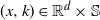 $(x,k)\in \mathbb{R}^d \times \mathbb{S}$
, we know that
 \begin{equation} \mathcal{A}\psi(x,k) = \langle\nabla\psi(x,k), g(x,k)\rangle + \mathcal{J}\psi(x,k) + Q\psi(x,k),\end{equation}
where the operator
 $\mathcal{J}$
is defined as
 \begin{equation} \mathcal{J}\psi(x,k) = \int_{\mathbb{R}^d_0}[\psi(x+\sigma z,k) - \psi(x,k) - \langle\nabla\psi(x,k),\sigma z\rangle\mathbf{1}_{\{|z|\leqslant 1\}}]\frac{d_{\alpha}}{|z|^{d+\alpha}}\,\mathrm{d}z,\end{equation}
with
 $\mathbb{R}^d_0=\mathbb{R}^d \setminus \{0\}$
, and
 $Q\psi(x,k)$
given by
 \begin{equation*} Q\psi(x,k) = \sum_{j\neq k}q_{kj}[\psi(x,j)-\psi(x,k)] = \sum_{j\in\mathbb{S}}q_{kj}\psi(x,j) = [Q\psi(x,\cdot)]_k,\end{equation*}
where
 $[Q \psi(x,\cdot)]_k$
is the kth element of the vector
 $Q \psi(x,\cdot)$
.
We now consider the following Stein equation: for any function
 $h\in \mathcal{C}_\mathrm{b}^1(\mathbb{R}^d \times \mathbb{S},\mathbb{R})$
,
 \begin{equation} \mathcal{A}f_h(x,k) = h(x,k)-\mu(h),\end{equation}
where
 $\mathcal{A}$
and
 $\mu$
are respectively the infinitesimal generator and invariant measure for the process
 $(X_t,R_t)_{t\geqslant 0}$
. The following regularity results hold for the solution
 $f_h$
.
Lemma 4.1. Under Assumptions 1.1 and ‘1.2, with
 $\eta>0$
defined in (1.4), let
 $h\in\mathcal{C}_\mathrm{b}^1(\mathbb{R}^d\times\mathbb{S},\mathbb{R})$
and
 $f_h$
be the solution to Stein’s equation (4.5). For any
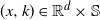 $(x,k)\in\mathbb{R}^d\times\mathbb{S}$
, there exists some positive constant C such that
 $|f_h(x,k)| \leqslant C(1+|x|^{\kappa_2})$
and
 $\|\nabla f_h(x,k)\|_{\infty} \leqslant C$
, where the constant
 $\kappa_2$
is specified in Assumption 1.2.
4.1. Proof of Theorem 2.2
We prove Theorem 2.2 by Itô’s formula and the martingale CLT. The verification of the martingale CLT conditions is highly nontrivial.
Proof of Theorem
2.2. For the process
 $(X_t,R_t)_{t\geqslant 0}$
in the system in (1.1) with
 $(X_0,R_0)=(x,k)$
, by Itô’s formula for
 $f_h$
, which is the solution of Stein’s equation (4.5), we have
 \begin{align*} f_h(X_t^{x,k},R_t^k)-f_h(x,k) & = \int_0^t\mathcal{A}f_h(X_s^{x,k},R_s^k)\,\mathrm{d}s + \mathcal{M}_{1,t} + \mathcal{M}_{2,t} \nonumber \\[2pt] & = \int_0^t[h(X_s^{x,k},R_s^k)-\mu(h)]\,\mathrm{d}s + \mathcal{M}_{1,t} + \mathcal{M}_{2,t}, \end{align*}
where
 $\mathcal{M}_{1,t}$
and
 $\mathcal{M}_{2,t}$
are martingales:
 \begin{align*} \mathcal{M}_{1,t} & = \int_0^t\int_{\mathbb{R}_0^d}\big[f_h\big(X_{s-}^{x,k}+\sigma z,R_{s-}^k\big) - f_h\big(X_{s-}^{x,k},R_{s-}^k\big)\big]\,\widetilde{N}_2(\mathrm{d}s,\mathrm{d}z), \\[2pt] \mathcal{M}_{2,t} & = \int_0^t\int_{\mathbb{R}_0}\big[f_h\big(X_{s-}^{x,k},R_{s-}^k+\ell(R_{s-}^k,\tilde{z})\big) - f_h\big(X_{s-}^{x,k},R_{s-}^k\big)\big]\,\widetilde{N}_1(\mathrm{d}s,\mathrm{d}\tilde{z}), \end{align*}
with
 $\widetilde{N}_1$
the compensated Poisson measure for
 $N_1$
, and
 $\ell$
as defined in (4.1). This implies that
 \begin{align*} \sqrt{t}\bigg[\frac{1}{t}\int_0^t\delta_{(X_s^{x,k},R_s^k)}(h)\,\mathrm{d}s - \mu(h)\bigg] & = \frac{1}{\sqrt{t}\,}\int_0^t\big[h\big(X_s^{x,k},R_s^k\big)-\mu(h)\big]\,\mathrm{d}s \\[4pt] & = \frac{1}{\sqrt{t}\,}\big[f_h\big(X_t^{x,k},R_t^k\big)-f_h(x,k)\big] - \frac{1}{\sqrt{t}\,}(\mathcal{M}_{1,t}+\mathcal{M}_{2,t}). \end{align*}
From the estimates for
 $|f_h(x,k)|$
and
 $\mathbb{E}|X_t^{x,k}|^{\kappa_2}$
in Lemmas 4.1 and 3.2 respectively, we get
 \begin{equation*} |\mathbb{E}f_h\big(X_t^{x,k},R_t^k\big)| \leqslant \mathbb{E}(1+|X_t^{x,k}|^{\kappa_2}) \leqslant C(1+|x|^{\kappa_2}), \end{equation*}
which implies that
 $\mathbb{E}|({1}/{\sqrt{t}})[f_h(X_t^{x,k},R_t^k)-f_h(x,k)]| \to 0$
as
 $t \to \infty$
. It follows from the estimates for
 $|f_h(x,k)|$
and
 $\|\nabla f_h\|_{\infty}$
in Lemma 4.1 that
 \begin{align*} & \int_{\mathbb{R}_0^d}|f_h(x+\sigma z)-f_h(x)|^2\,\nu(\mathrm{d}z) \nonumber \\[3pt] & \qquad = \int_{0<|z|\leqslant 1}\bigg|\int_0^1\langle\nabla f_h(x+r\sigma z),\sigma z\rangle\, \mathrm{d}r\bigg|^2\, \nu(\mathrm{d}z) + \int_{|z|>1}|f_h(x+\sigma z)-f_h(x)|^2\,\nu(\mathrm{d}z) \nonumber \\[3pt] & \qquad \leqslant C\int_{0<|z|\leqslant 1}|z|^2\,\nu(\mathrm{d}z) + C\int_{|z|>1}(1+|x|^{2\kappa_2}+|z|^{2\kappa_2})\, \nu(\mathrm{d}z) \nonumber \\[3pt] & \qquad \leqslant C(1+|x|^{2\kappa_2}), \end{align*}
where the last two inequalities hold since
 $2\kappa_2<\kappa_1<\alpha$
and
 $\int_{\mathbb{R}_0^d}(1\wedge|z|^{\kappa_1})\,\nu(\mathrm{d}z)<\infty$
. Combining this with
 \begin{equation*} \int_{[0,M]}|f_h(x,k+\ell(k,\tilde{z}))-f_h(x,k)|^2\,\mathrm{d}\tilde{z} \leqslant C(1+|x|^{2\kappa_2}) \end{equation*}
implies that
 \begin{align} \mathcal{V}(f_h) & \, :\!= \, \int_{\mathbb{R}^d\times\mathbb{S}}\int_{\mathbb{R}_0^d}|f_h(x+\sigma z,k)-f_h(x,k)|^2\,\nu(\mathrm{d}z)\, \mathrm{d}\mu(x,k) \nonumber \\[3pt] & \quad + \int_{\mathbb{R}^d\times\mathbb{S}}\int_{\mathbb{R}_0}|f_h(x,k+\ell(k,\tilde{z}))-f_h(x,k)|^2\, \mathrm{d}\tilde{z}\,\mathrm{d}\mu(x,k) \nonumber \\[3pt] & \leqslant C\mu(1+|x|^{2\kappa_2}) < \infty, \end{align}
where the inequality holds since
 $2\kappa_2<\kappa_1$
and
 $\mu(|x|^{\kappa_1})<\infty$
in Proposition A.1.
To make the notation simpler, for
 $i=1,2,\ldots,\lfloor t \rfloor$
we write
 \begin{align*} U_i & = \int_{i-1}^i\int_{\mathbb{R}_0^d}\Big[f_h\Big(X_{s-}^{x,k}+\sigma z,R_{s-}^k\Big) - f_h\Big(X_{s-}^{x,k},R_{s-}^k\Big)\Big]\,\widetilde{N}_2(\mathrm{d}s,\mathrm{d}z) \nonumber \\[3pt] & \quad + \int_{i-1}^i\int_{\mathbb{R}_0}\Big[f_h\Big(X_{s-}^{x,k},R_{s-}^k+\ell(R_{s-}^k,\tilde{z})\Big) - f_h\Big(X_{s-}^{x,k},R_{s-}^k\Big)\Big]\,\widetilde{N}_1(\mathrm{d}s,\mathrm{d}\tilde{z}), \nonumber \\[3pt] U_{\lfloor t\rfloor+1} & = \int_{\lfloor t\rfloor}^t\int_{\mathbb{R}_0^d}\Big[f_h\Big(X_{s-}^{x,k}+\sigma z,R_{s-}^k\Big) - f_h\Big(X_{s-}^{x,k},R_{s-}^k\Big)\Big]\,\widetilde{N}_2(\mathrm{d}s,\mathrm{d}z) \nonumber \\[3pt] & \quad + \int_{\lfloor t\rfloor}^t\int_{\mathbb{R}_0}\Big[f_h\Big(X_{s-}^{x,k},R_{s-}^k+\ell(R_{s-}^k,\tilde{z})\Big) - f_h\Big(X_{s-}^{x,k},R_{s-}^k\Big)\Big]\,\widetilde{N}_1(\mathrm{d}s,\mathrm{d}\tilde{z}). \end{align*}
Then,
 \begin{equation*} \frac{1}{\sqrt{t}\,}(\mathcal{M}_{1,t}+\mathcal{M}_{2,t}) = \frac{1}{\sqrt{t}\,}\sum_{i=1}^{\lfloor t\rfloor + 1}U_i. \end{equation*}
We know that the
 $U_i$
are martingale differences and
 $\mathbb{E} U_i^2 <\infty$
, which can be obtained similarly with (4.6) for all
 $i=1,2,\ldots,\lfloor t\rfloor+1$
. We claim that
 \begin{align} \lim_{t\to\infty}\mathbb{E}\bigg(\max_{1\leqslant i\leqslant\lfloor t\rfloor+1} \frac{1}{\mathcal{V}(f_h)t}|U_i|^2\bigg) = 0, \nonumber \\[-30pt] \end{align}
 \begin{align} \lim_{t\to\infty}\mathbb{E}\Bigg|\sum_{i=1}^{\lfloor t\rfloor+1}\frac{1}{\mathcal{V}(f_h)t}|U_i|^2-1\Bigg|^2 = 0. \end{align}
We know that (4.7) and (4.8) imply that
 \begin{equation*} \mathbb{E}\bigg(\max_{1\leqslant i\leqslant\lfloor t\rfloor+1}\frac{1}{\sqrt{\mathcal{V}(f_h)t}\,}|U_i|\bigg) \to 0 \quad \text{and} \quad \sum_{i=1}^{\lfloor t\rfloor+1}\frac{1}{\mathcal{V}(f_h)t}|U_i|^2 \stackrel{\mathrm{p}}{\longrightarrow} 1 \end{equation*}
as t tends to infinity. Applying the martingale CLT in [Reference Sethuraman29, Theorem 2], due to [Reference Mcleish24], we have
 \begin{equation*} \frac{1}{\sqrt{\mathcal{V}(f_h)t}\,}\sum_{i=1}^{\lfloor t\rfloor+1}U_i \Rightarrow \mathcal{N} (0,1) \quad \text{as } t \to \infty. \end{equation*}
Then, we know that
 \begin{equation*} \sqrt{t}\bigg[\frac{1}{t}\int_0^t\delta_{(X_s^{x,k},R_s^k)}(h)\,\mathrm{d}s - \mu(h)\bigg] \Rightarrow \mathcal{N}(0,\mathcal{V}(f_h)) \quad \text{as } t \to \infty. \end{equation*}
It remains to show (4.7) and (4.8). For (4.7), we have
 \begin{align*} \mathbb{E}\Big(\max_{1\leqslant i\leqslant\lfloor t\rfloor+1}|U_i|^2\Big) & = \mathbb{E}\Big(\max_{1\leqslant i\leqslant\lfloor t\rfloor+1}(|U_i|^2\mathbf{1}_{\{|U_i|^2\leqslant \sqrt{t}\}} + |U_i|^2\mathbf{1}_{\{|U_i|^2 > \sqrt{t}\}})\Big) \nonumber \\[3pt] & \leqslant \mathbb{E}\Big(\max_{1\leqslant i\leqslant\lfloor t\rfloor+1}|U_i|^2\mathbf{1}_{\{|U_i|^2\leqslant\sqrt{t}\}}\Big) + \mathbb{E}\Big(\max_{1\leqslant i\leqslant\lfloor t\rfloor+1}|U_i|^2\mathbf{1}_{\{|U_i|^2>\sqrt{t}\}}\Big) \nonumber \\[3pt] & \leqslant \sqrt{t} + (\lfloor t\rfloor+1)\max_{1\leqslant i\leqslant\lfloor t\rfloor+1} \mathbb{E}\big[|U_i|^2\mathbf{1}_{\{|U_i|^2>\sqrt{t}\}}\big]. \end{align*}
Thus, as
 $t \to \infty$
, we obtain
 \begin{equation*} \mathbb{E}\bigg(\max_{1\leqslant i\leqslant\lfloor t\rfloor+1}\frac{1}{\mathcal{V}(f_h)t}|U_i|^2\bigg) \leqslant \frac{1}{\mathcal{V}(f_h)t}\Big(\sqrt{t} + (\lfloor t\rfloor+1)\max_{1\leqslant i\leqslant\lfloor t\rfloor+1}\mathbb{E}[|U_i|^2\mathbf{1}_{\{|U_i|^2>\sqrt{t}\}}]\Big) \to 0. \end{equation*}
It is easy to verify (4.8) by proving the equation
 \begin{equation} \lim_{t\to\infty}\mathbb{E}\Bigg|\sum_{i=1}^{\lfloor t\rfloor+1}\frac{1}{\mathcal{V}(f_h)t}|U_i|^2 - \frac{\lfloor t\rfloor+1}{t}\Bigg|^2 = 0. \end{equation}
Observe that
 \begin{align*} & \mathbb{E}\Bigg|\sum_{i=1}^{\lfloor t\rfloor+1}\frac{1}{\mathcal{V}(f_h)t}|U_i|^2 - \frac{\lfloor t\rfloor+1}{t}\Bigg|^2 \nonumber \\[3pt] & \quad = \mathbb{E}\Bigg|\frac{1}{t}\sum_{i=1}^{\lfloor t\rfloor+1} \bigg(\frac{1}{\mathcal{V}(f_h)}|U_i|^2-1\bigg)\Bigg|^2 \nonumber \\[3pt] & \quad = \underbrace{\frac{1}{t^2}\sum_{i=1}^{\lfloor t\rfloor+1} \mathbb{E}\bigg(\frac{1}{\mathcal{V}(f_h)}|U_i|^2-1\bigg)^2}_{\mathrm{I}} + \underbrace{\frac{2}{t^2}\sum_{i < j}\mathbb{E}\bigg[\bigg(\frac{1}{\mathcal{V}(f_h)}|U_i|^2-1\bigg) \bigg(\frac{1}{\mathcal{V}(f_h)}|U_j|^2-1\bigg)\bigg]}_{\mathrm{II}}. \end{align*}
Using Kunita’s inequality (see [Reference Applebaum1, Theorem 4.4.23]), with similar calculations for (4.6), there exists some constant
 $C>0$
such that
 \begin{align*} \mathbb{E}|U_i|^4 & \leqslant C\mathbb{E}\Bigg|\int_{i-1}^i\int_{\mathbb{R}_0^d}\big|f_h\big(X_{s-}^{x,k}+\sigma z,R_{s-}^k\big) - f_h\big(X_{s-}^{x,k},R_{s-}^k\big)\big|^2\,\nu(\mathrm{d}z)\,\mathrm{d}s\Bigg|^2 \nonumber \\[3pt] & \quad + C\mathbb{E}\int_{i-1}^i\int_{\mathbb{R}_0^d}\big|f_h\big(X_{s-}^{x,k}+\sigma z,R_{s-}^k\big) - f_h\big(X_{s-}^{x,k},R_{s-}^k\big)\big|^4\,\nu(\mathrm{d}z)\,\mathrm{d}s \nonumber \\[3pt] & \quad + C\mathbb{E}\bigg|\int_{i-1}^i\int_{[0,M]}\big|f_h\big(X_{s-}^{x,k},R_{s-}^k + \ell\big(R_{s-}^k,\tilde{z}\big)\big) - f_h\big(X_{s-}^{x,k},R_{s-}^k\big)\big|^2\, \mathrm{d}\tilde{z}\,\mathrm{d}s\bigg|^2 \nonumber \\[3pt] & \quad + C\mathbb{E}\int_{i-1}^i\int_{[0,M]}\big|f_h\big(X_{s-}^{x,k},R_{s-}^k + \ell\big(R_{s-}^k,\tilde{z}\big)\big) - f_h\big(X_{s-}^{x,k},R_{s-}^k\big)\big|^4\, \mathrm{d}\tilde{z}\,\mathrm{d}s \nonumber \\[3pt] & \leqslant C\mathbb{E}\big(1+|X_{i-1}^{x,k}|^{4\kappa_2}\big) \leqslant C(1+|x|^{4\kappa_2}), \end{align*}
where the second inequality holds from the fact
 $4\kappa_2 \leqslant \kappa_1$
and the last inequality holds from the estimate
 $\mathbb{E}|X_{i-1}^{x,k}|^{4\kappa_2}$
in Lemma 3.2. Combining this with Lemma 3.2 and the fact that
 $4\kappa_2 \leqslant \kappa_1<\alpha$
, we know that
 \begin{align*} \mathbb{E}\bigg(\frac{1}{\mathcal{V}(f_h)}|U_i|^2-1\bigg)^2 & = \mathbb{E}\bigg[\frac{1}{\mathcal{V}^2(f_h)}|U_i|^4 - \frac{2}{\mathcal{V}(f_h)}|U_i|^2+1\bigg] \\[3pt] & \leqslant C\big(1+\mathbb{E}|X_i^{x,k}|^{4\kappa_2}\big) \leqslant C\big(1+|x|^{4\kappa_2}\big), \end{align*}
which implies that
 \begin{equation*} \mathrm{I} = \frac{1}{t^2}\sum_{i=1}^{\lfloor t\rfloor+1}\mathbb{E}\bigg(\frac{1}{\mathcal{V}(f_h)}|U_i|^2-1\bigg)^2 \to 0 \quad \text{as } t \to \infty. \end{equation*}
As for II, for each i, it holds that, for some positive constant C,
 \begin{align*} \Bigg|\sum_{j=i+1}^{\lfloor t\rfloor+1}\mathbb{E}\bigg[\bigg(\frac{1}{\mathcal{V}(f_h)}|U_j|^2-1\bigg) \mid \mathcal{F}_{i}\bigg]\Bigg| & = \frac{1}{\mathcal{V}(f_h)}\Bigg|\sum_{j=i+1}^{\lfloor t\rfloor+1}\mathbb{E}\big[(|U_j|^2-\mathcal{V}(f_h)) \mid \mathcal{F}_{i}\big]\Bigg| \\ & \leqslant \int_{0}^{\lfloor t\rfloor+1}\Big(1+|X_i^{x,k}|^{2\kappa_2}\Big)\mathrm{e}^{-cs}\,\mathrm{d}s \leqslant C\Big(1+|X_i^{x,k}|^{2\kappa_2}\Big), \end{align*}
where
 $\mathcal{F}_{i}$
is the filtration generated by the process
 $(X_t,R_t)_{t\geqslant 0}$
at time
 $t=i$
, and the first inequality is by Proposition A.1 and the fact that
 $2\kappa_2<\kappa_1$
. Hence, we can obtain that
 \begin{align*} |\mathrm{II}| & = \frac{2}{t^2}\Bigg|\sum_{i=1}^{\lfloor t\rfloor}\sum_{j=i+1}^{\lfloor t\rfloor+1} \mathbb{E}\bigg\{\bigg(\frac{1}{\mathcal{V}(f_h)}|U_i|^2-1\bigg) \mathbb{E}\bigg[\bigg(\frac{1}{\mathcal{V}(f_h)}|U_j|^2-1\bigg) \mid \mathcal{F}_{i}\bigg]\bigg\}\Bigg| \\ & \leqslant \frac{C}{t^2}\sum_{i=1}^{\lfloor t\rfloor} \mathbb{E}\bigg\{\bigg|\frac{1}{\mathcal{V}(f_h)}|U_i|^2-1\bigg|\big(1+|X_i^{x,k}|^{2\kappa_2}\big)\bigg\} \\ & \leqslant \frac{C}{t^2}\sum_{i=1}^{\lfloor t\rfloor}\bigg[ \mathbb{E}\bigg|\frac{1}{\mathcal{V}(f_h)}|U_i|^2-1\bigg|^2\bigg]^{1/2} \big[1+\mathbb{E}|X_i^{x,k}|^{4\kappa_2}\big]^{1/2} \to 0 \quad \text{as } t \to \infty. \end{align*}
Combining the estimates for I and II, (4.9) holds. The proof is complete.
4.2. Proof of Theorem 2.3
We shall prove the MDP by the criterion in [Reference Wu34, Theorem 2.6].
Proof of Theorem
2.3. According to the criterion for MDP in [Reference Wu34, Theorem 2.6], we need to show that the semigroup
 $P_t$
associated with the process
 $(X_t,R_t)_{t\geqslant 0}$
is strong Feller, topologically irreducible, and satisfies a Lyapunov condition. The process
 $(X_t,R_t)_{t\geqslant 0}$
defined in (1.1) is strong Feller and irreducible, which can be obtained from the discussions in [Reference Xi35, Theorems 3.2 and 4.5], [Reference Yin and Zhu39, Theorem 2.24], and [Reference Xi37, Theorems 5.6 and 6.3], and the Lyapunov condition is implied by (A.4).
For
 $h\in\mathcal{C}_\mathrm{b}^1(\mathbb{R}^d\times\mathbb{S},\mathbb{R})$
, it follows from [Reference Wu34, Theorem 2.6] that
 \begin{equation*} \mathbb{P}\bigg(\frac{1}{a_t\sqrt{t}\,}\int_0^t[h(X_s^{x,k},R_s^k)-\mu(h)]\,\mathrm{d}s \in \ \cdot \,\bigg) \end{equation*}
satisfies the large deviation principle with speed
 $a_t^{-2}$
and rate function
 $I_h(z)={z^2}/{2\mathcal{H}(h)}$
, with
 $\mathcal{H}(h) = 2\int_0^{\infty}\langle P_t h,h-\mu(h)\rangle_{\mu}\,\mathrm{d}t$
, that is,
 \begin{align*} -\inf_{z\in\it{\unicode{x00C5}}}I_h(z) & \leqslant \liminf_{t\to\infty}\frac{1}{a_t^2}\log\mathbb{P}\bigg( \frac{\sqrt{t}}{a_t}\big[\mathcal E^{x,k}_t(h)-\mu(h)\big] \in A\bigg) \\ & \leqslant \limsup_{t\to\infty}\frac{1}{a_t^2}\log\mathbb{P}\bigg( \frac{\sqrt{t}}{a_t}\big[\mathcal E^{x,k}_t(h)-\mu(h)\big] \in A\bigg) \leqslant -\inf_{z\in\bar{A}}I_h(z), \end{align*}
where
 $\bar{A}$
and
 $\it{\unicode{x00C5}}$
are the closure and interior of set A respectively.
We claim that
 \begin{equation} \mathcal{H}(h) = \mathcal{V}(f_h), \end{equation}
where
 $f_h$
is the solution to Stein’s equation (4.5). Then the desired result holds.
Now, we show that the claim (4.10) holds. With some calculations, we have
 \begin{align*} & \frac{1}{t}\mathbb{E}^{\mu}\bigg(\int_0^t\Big[h\big(X_s^{x,k},R_s^k\big)-\mu(h)\Big]\,\mathrm{d}s\bigg)^2 \\[3pt] & \qquad = \frac{2}{t}\mathbb{E}^{\mu}\bigg(\int_0^t\int_0^u\Big[h\big(X_s^{x,k},R_s^k\big)-\mu(h)\Big]\Big[h\big(X_u^{x,k},R_u^k\big)-\mu(h)\Big]\, \mathrm{d}s\,\mathrm{d}u\bigg) \\ & \qquad = \frac{2}{t}\int_0^t\int_0^u\mathbb{E}^{\mu}\Big\{h\big(X_s^{x,k},R_s^k\big)\mathbb{E}\Big\{\Big[h\big(X_u^{x,k},R_u^k\big)-\mu(h)\Big] \mid \mathcal{F}_s\Big\}\Big\}\,\mathrm{d}s\,\mathrm{d}u, \end{align*}
where
 $\mathcal{F}_s$
is the filtration generated by the process
 $(X_t,R_t)_{t\geqslant 0}$
at time
 $t=s$
; the second equality holds from conditional probability and the fact that
 \begin{multline*} \int_0^t\int_0^u\mathbb{E}^{\mu}\Big\{\mu(h)\mathbb{E}\big\{\big[h\big(X_u^{x,k},R_u^k\big)-\mu(h)\big] \mid \mathcal{F}_s\big\}\big\}\, \mathrm{d}s\,\mathrm{d}u \\ = \mu(h)\int_0^t\int_0^u\mathbb{E}^{\mu}\big\{h\big(X_u^{x,k},R_u^k\big)-\mu(h)\big\}\,\mathrm{d}s\,\mathrm{d}u = 0. \end{multline*}
Furthermore, for all
 $0\leqslant s \leqslant u<\infty$
, we have
 \begin{align*} & \mathbb{E}^{\mu}\big\{h\big(X_s^{x,k},R_s^k\big)\mathbb{E}\big\{\big[h\big(X_u^{x,k},R_u^k\big)-\mu(h)\big] \mid \mathcal{F}_s\big\}\big\} \\ & \qquad = \mathbb{E}^{\mu}\big\{h\big(X_s^{x,k},R_s^k\big)\big[P_{u-s}h\big(X_s^{x,k},R_s^k\big) - \mu(h)\big]\big\} \\ & \qquad = \int_{\mathbb{R}^d\times\mathbb{S}}h(y,k)\big[P_{u-s}h(y,k)-\mu(h)\big]\,\mathrm{d}\mu(y,k), \end{align*}
which implies that
 \begin{align*} & \frac{2}{t}\int_0^t\int_0^u\mathbb{E}^{\mu}\big\{h\big(X_s^{x,k},R_s^k\big)\mathbb{E}\big\{\big[h(X_u^{x,k},R_u^k)-\mu(h)\big] \mid \mathcal{F}_s\big\}\big\}\,\mathrm{d}s\,\mathrm{d}u \\ & \qquad = \int_{\mathbb{R}^d\times\mathbb{S}}h(y,k)\frac{2}{t}\int_0^t\int_0^u \big[P_{u-s}h(y,k)-\mu(h)\big]\,\mathrm{d}s\,\mathrm{d}u\,\mathrm{d}\mu(y,k) \\ & \qquad = \int_{\mathbb{R}^d\times\mathbb{S}}h(y,k)\frac{2}{t}\int_0^t\int_0^u \big[P_{\tilde{s}}h(y,k)-\mu(h)\big]\, \mathrm{d}\tilde{s}\,\mathrm{d}u\,\mathrm{d}\mu(y,k). \end{align*}
Using L’Hôpital’s rule, we have
 \begin{multline*} \lim_{t\to\infty}\int_{\mathbb{R}^d\times\mathbb{S}}h(y,k)\frac{2}{t}\int_0^t\int_0^u [P_{\tilde{s}}h(y,k)-\mu(h)]\,\mathrm{d}\tilde{s}\,\mathrm{d}u\,\mathrm{d}\mu(y,k) \\ = 2\int_{\mathbb{R}^d\times\mathbb{S}}h(y,k)\int_0^{\infty}[P_{\tilde{s}}h(y,k)-\mu(h)]\, \mathrm{d}\tilde{s}\,\mathrm{d}\mu(y,k), \end{multline*}
that is,
 \begin{equation} \frac{1}{t}\mathbb{E}^{\mu}\bigg(\int_0^t\big[h(X_s^{x,k},R_s^k)- \mu(h)\big]\,\mathrm{d}s\bigg)^2 \to \mathcal{H}(h) \quad \text{as } t \to \infty. \end{equation}
Indeed,
 $\mathcal{H}(h)$
can also be expressed as
 \begin{equation*} \mathcal{H}(h) = 2\int_0^{\infty}\langle P_th,h-\mu(h)\rangle_{\mu}\,\mathrm{d}t = 2\int_0^{\infty}\langle P_th-\mu(h),h\rangle_{\mu}\,\mathrm{d}t. \end{equation*}
Using Itô’s formula and Stein’s equation (4.5), we have
 \begin{align*} f_h(X_t^{x,k},R_t^k)-f_h(x,k) & = \int_0^t\mathcal{A}f_h\big(X_s^{x,k},R_s^k\big)\,\mathrm{d}s + \mathcal{M}_{1,t} + \mathcal{M}_{2,t} \\ & = \int_0^t\big[h\big(X_s^{x,k},R_s^k\big)-\mu(h)\big]\,\mathrm{d}s + \mathcal{M}_{1,t} + \mathcal{M}_{2,t}. \end{align*}
Combining this with the ergodic theorem and the fact that
 $\mathbb{E}\big|[f_h(X_t^{x,k},R_t^k)-f_h(x,k)]/{\sqrt{t}}\big|\to0$
as
 $t\to\infty$
yields
 \begin{align} & \frac{1}{t}\mathbb{E}^{\mu}\bigg(\int_0^t\big[h\big(X_s^{x,k},R_s^k\big)-\mu(h)\big]\,\mathrm{d}s\bigg)^2 \nonumber \\ & \quad = \mathbb{E}^{\mu}\bigg(\frac{1}{\sqrt{t}\,}\big[f_h\big(X_t^{x,k},R_t^k\big) - f_h(x,k) - \mathcal{M}_{1,t} - \mathcal{M}_{2,t}\big]\bigg)^2 \to \mathcal{V}(f_h) \quad \text{as } t\to\infty. \end{align}
Thus, we know that
 $\mathcal{H}(h)=\mathcal{V}(f_h)$
by (4.11) and (4.12), so the claim (4.10) holds. The proof is complete.
5. Proof of Theorem 2.4
In order to determine the variance in Theorem 2.4, we need to study the second Stein equation
 \begin{equation} \mathcal{A}_{\gamma} f_{\gamma,h}(x,k)=h(x,k)-\mu_{\gamma}(h),\end{equation}
where
 $\mathcal{A}_{\gamma}$
is defined as
 \begin{equation} \mathcal{A}_{\gamma} f_{\gamma,h}(x,k)=\bar{P}_{\gamma} f_{\gamma,h}(x,k)-f_{\gamma,h}(x,k).\end{equation}
It is easy to verify that the solution of the equation (5.1) is
 \begin{equation} f_{\gamma,h}(x,k) = -\sum_{i=0}^{\infty} \bar{P}^i_{\gamma}(h(x,k)-\mu_{\gamma}(h)),\end{equation}
because
 $\bar{P}_{\gamma}f_{\gamma,h}(x,k) = -\sum_{i=1}^{\infty}\bar{P}^i_{\gamma}(h(x,k)-\mu_{\gamma}(h))$
.
Proof of Theorem
2.4. (i) From Proposition A.2, we know that the EM scheme
 $(Y_{t_n}^{x,k},R_{t_n}^k)_{n\in \mathbb{N}_0}$
is exponentially ergodic under the weighted total variation distance
 $\|\cdot\|_{\mathrm{1+V^{(1)}}}$
and
 $\mu_{\gamma}(V^{(1)})\leqslant C$
with
 $V^{(1)}$
as in (A.1). It follows from [Reference Jones15, Theorem 9] that, for any function h satisfying
 $|h|\leqslant V^{(1)}$
and any initial distribution
 $(Y_{0},R_0)$
,
 $\sqrt{n}\big[\mathcal{E}_{n,\gamma}^{x,k}(h) - \mu_{\gamma}(h)\big] \Rightarrow \mathcal{N}(0,\sigma_h^2)$
with
 \begin{equation} \sigma_h^2 = \langle h-\mu_{\gamma}(h),h-\mu_{\gamma}(h)\rangle_{\mu_{\gamma}} + 2\sum_{i=1}^{\infty}\langle\bar{P}^i_{\gamma}h,h-\mu_{\gamma}(h)\rangle_{\mu_{\gamma}}. \end{equation}
We give some calculations for the variance of
 $\sqrt{n}\big[\mathcal{E}_{n,\gamma}^{x,k}(h)-\mu_{\gamma}(h)\big]$
. Since
 $\mathbb{E}\big[\sqrt{n}\big(\mathcal{E}_{n,\gamma}^{x,k}(h)-\mu_{\gamma}(h)\big)\big]=0$
, we have
 \begin{align} & \mathbb{E}\big|\sqrt{n}\big[\mathcal{E}_{n,\gamma}^{x,k}(h)-\mu_{\gamma}(h)\big]\big|^2 \nonumber \\ & \qquad = \mathbb{E}\Bigg|\frac{1}{\sqrt{n}\,}\sum_{i=0}^{n-1}\big[h\big(Y^{x,k}_{t_i},R^{k}_{t_i}\big) - \mu_{\gamma}(h)\big]\Bigg|^2 \nonumber \\ & \qquad = \frac{1}{n}\sum_{i=0}^{n-1}\mathbb{E}\big|h\big(Y^{x,k}_{t_i},R^{k}_{t_i}\big)-\mu_{\gamma}(h)\big|^2 \nonumber \\ & \qquad\quad + \frac{2}{n}\sum_{i=1}^{n-1}\sum_{j=0}^{i-1} \mathbb{E}\big\{\big[h\big(Y^{x,k}_{t_i},R^{k}_{t_i}\big)-\mu_{\gamma}(h)\big] \big[h\big(Y^{x,k}_{t_j},R^{k}_{t_j}\big)-\mu_{\gamma}(h)\big]\big\}. \end{align}
We aim to deal with the second term on the right-hand side of (5.5). By the conditional expectation, we have
 \begin{align} & \frac{2}{n}\sum_{i=1}^{n-1}\sum_{j=0}^{i-1} \mathbb{E}\big\{\big[h\big(Y^{x,k}_{t_i},R^{k}_{t_i}\big)-\mu_{\gamma}(h)\big] \big[h\big(Y^{x,k}_{t_j},R^{k}_{t_j}\big) - \mu_{\gamma}(h)\big]\big\} \nonumber \\ & \quad = \frac{2}{n}\sum_{i=1}^{n-1}\sum_{j=0}^{i-1} \mathbb{E}\big\{\big[h\big(Y^{x,k}_{t_j},R^{k}_{t_j}\big)-\mu_{\gamma}(h)\big] \mathbb{E}\big[\big(h\big(Y^{x,k}_{t_i},R^{k}_{t_i}\big)-\mu_{\gamma}(h)\big) \mid \bar{\mathcal{F}}_{t_j}\big]\big\} \nonumber \\ & \quad = \frac{2}{n}\sum_{j=0}^{n-2}\mathbb{E}\Bigg\{\big[h\big(Y^{x,k}_{t_j},R^{k}_{t_j}\big)-\mu_{\gamma}(h)\big] \mathbb{E}\Bigg[\sum_{i=j+1}^{n-1}\big(h\big(Y^{x,k}_{t_i},R^{k}_{t_i}\big)-\mu_{\gamma}(h)\big) \mid \bar{\mathcal{F}}_{t_j}\Bigg]\Bigg\} \nonumber \\ & \quad = \frac{2}{n}\sum_{j=0}^{n-2}\mathbb{E}\Bigg\{\big[h\big(Y^{x,k}_{t_j},R^{k}_{t_j}\big)-\mu_{\gamma}(h)\big] \Bigg[\sum_{i=1}^{n-1-j}\bar{P}_{\gamma}^i\big(h\big(Y^{x,k}_{t_j},R^{k}_{t_j}\big)-\mu_{\gamma}(h)\big) \mid \bar{\mathcal{F}}_{t_j}\Bigg]\Bigg\} \nonumber \\ & \quad \to 2\sum_{i=1}^{\infty}\langle\bar{P}^i_{\gamma}[h(x,k)-\mu_{\gamma}(h)], h(x,k)-\mu_{\gamma}(h)\rangle_{\mu_{\gamma}} \quad \text{as } n\to \infty, \end{align}
where
 $\bar{\mathcal{F}}_s$
is the filtration generated by the EM scheme
 $(Y_{t_n},R_{t_n})_{n\in \mathbb{N}_0}$
at time s.
Combining (5.5) and (5.6), as
 $n\to \infty$
we know that
 \begin{equation*} \mathbb{E}\big|\sqrt{n}\big[\mathcal{E}_{n,\gamma}^{x,k}(h)-\mu_{\gamma}(h)\big]\big|^2 \to \langle h-\mu_{\gamma}(h),h-\mu_{\gamma}(h)\rangle_{\mu_{\gamma}} + 2\sum_{i=1}^{\infty}\langle\bar{P}^i_{\gamma}h,h-\mu_{\gamma}(h)\rangle_{\mu_{\gamma}}, \end{equation*}
which implies that (5.4) holds.
Since
 $\langle\mu_{\gamma}(h),h-\mu_{\gamma}(h)\rangle_{\mu_{\gamma}}=0$
, using (5.3) it is easy to verify that
 \begin{align*} \widetilde{\mathcal{V}}(f_{\gamma,h}) & = \langle f_{\gamma,h},f_{\gamma,h}\rangle_{\mu_{\gamma}} - \langle\bar{P}_{\gamma}f_{\gamma,h},\bar{P}_{\gamma}f_{\gamma,h}\rangle_{\mu_{\gamma}} \\ & = \langle h-\mu_{\gamma}(h),h-\mu_{\gamma}(h)\rangle_{\mu_{\gamma}} + 2\sum_{i=1}^{\infty} \big\langle\bar{P}^i_{\gamma}h,h-\mu_{\gamma}(h)\big\rangle_{\mu_{\gamma}} = \sigma_h^2. \end{align*}
(ii) It follows from Proposition A.2 that the EM scheme
 $\big(Y_{t_n}^{x,k},R_{t_n}^k\big)_{n\in \mathbb{N}_0}$
has exponential ergodicity. It follows from [Reference Wu34, Remark 2.17] that
 $\bar{P}^n_{\gamma}$
has a spectral gap near its largest eigenvalue 1, which implies that 1 is an isolated eigenvalue. Since
 $\bar{P}^i_{\gamma} c=c$
for all
 $i \in \mathbb{N}_0$
, 1 is an eigenvalue of
 $\bar{P}^i_{\gamma}$
for all
 $i \in \mathbb{N}_0$
. If there exists some function
 $\hat{f}$
satisfying
 $0\neq \hat{f}(x,k) \leqslant 1+V^{(1)}(x,k)$
for all
 $x\in \mathbb{R}^d$
such that
 $\bar{P}^{k_1}_{\gamma} \hat{f}=\lambda \hat{f}$
for some
 $k_1 \in \mathbb{N}_0$
and
 $\lambda\in\mathbb{C}$
with
 $|\lambda|=1$
, then
 $\lambda^{\tilde{n}}\hat{f}=\bar{P}^{\tilde{n}k_1}_{\gamma}\hat{f}\to\mu_{\gamma}(\hat{f})$
as
 $\tilde{n} \to \infty$
, so that
 $\hat{f}$
has to be constant and
 $\lambda=1$
. Thus, 1 is a simple eigenvalue and the only eigenvalue with modulus 1 for
 $\bar{P}_{\gamma}^n$
.
For
 $h\in \mathcal{C}_\mathrm{b}^1(\mathbb{R}^d \times \mathbb{S},\mathbb{R})$
, it follows from [Reference Wu33, Theorem 2.1] that
 \begin{equation*} \mathbb{P}\bigg(\frac{\sqrt{n}}{a_n}\big[\mathcal{E}_{n,\gamma}^{x,k}(h)-\mu_{\gamma}(h)\big] \in \ \cdot \,\bigg) \end{equation*}
satisfies the large deviation principle with speed
 $a_n^{-2}$
and rate function
 $I_h(z)={z^2}/{2\widetilde{\mathcal{V}}(f_{\gamma,h})}$
, with
 $\widetilde{\mathcal{V}}(f_{\gamma,h})$
as in (2.4), that is,
 \begin{align*} -\inf_{z\in\it{\unicode{x00C5}}}\frac{z^2}{2\widetilde{\mathcal{V}}(f_{\gamma,h})} & \leqslant \liminf_{n\to\infty}\frac{1}{a_n^2}\log\mathbb{P}\bigg(\frac{\sqrt{n}}{a_n} \big[\mathcal{E}_{n,\gamma}^{x,k}(h)-\mu_{\gamma}(h)\big] \in A\bigg) \\ & \leqslant \limsup_{n\to\infty}\frac{1}{a_n^2}\log\mathbb{P}\bigg(\frac{\sqrt{n}}{a_n} \big[\mathcal{E}_{n,\gamma}^{x,k}(h)-\mu_{\gamma}(h)\big] \in A\bigg) \leqslant -\inf_{z\in\bar{A}}\frac{z^2}{2\widetilde{\mathcal{V}}(f_{\gamma,h})}, \end{align*}
where
 $\bar{A}$
and
 $\it{\unicode{x00C5}}$
are the closure and interior of set A respectively. The proof is complete.
Appendix A. Exponential ergodicity and moment estimates
In this section we first show that the process
 $(X_t,R_t)_{t \geqslant 0}$
and its EM scheme
 $(Y_{t_n},R_{t_n})_{n \in \mathbb{N}_0}$
both have exponential ergodicities under the weighted total variation distance, and then give the moment estimates.
A.1. Exponential ergodicity
Proposition A.1. Under Assumptions 1.1 and 1.2, the process
 $(X_t,R_t)_{t \geqslant 0}$
is exponentially ergodic with ergodic measure
 $\mu$
. More precisely, for any
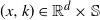 $(x,k)\in \mathbb{R}^d \times \mathbb{S}$
, there exist some positive constants c and C, independent of x, k, and t, satisfying
 \begin{equation*} \sup_{\psi\leqslant 1+|\cdot|^{\kappa_j}}\{P_{t} \psi(x,k) -\mu(\psi)\} \leqslant C(1+|x|^{\kappa_j})\mathrm{e}^{-ct}, \end{equation*}
where the
 $\kappa_j$
with
 $j\in \{1,2\}$
are as in Assumption 1.2. In addition,
 $\mu(|x|^{\kappa_j})\leqslant C$
.
To get the exponential ergodicity for the EM scheme
 $(Y_{t_n},R_{t_n})_{n\in \mathbb{N}_0}$
, we need the following relationship between
 $\mathcal{A}$
and
 $\mathcal{A}_{\gamma}$
defined in (4.3) and (5.2) respectively.
Lemma A.1. For
 $\psi\in\mathcal{C}^2(\mathbb{R}^d,\mathbb{R}) \cap \mathcal{D}(\mathcal{A}) \cap \mathcal{D}(\mathcal{A}_{\gamma})$
,
 $\mathcal{A}_{\gamma}\psi(x,k) = \gamma\mathcal{A}\psi(x,k) + \mathcal{R}_1 + \mathcal{R}_2 + \mathcal{R}_3 + \mathcal{R}_4$
, where the remainders are defined as
 \begin{align*} \mathcal{R}_1 & = (\mathrm{e}^{\gamma Q}-\mathrm{I}_d-\gamma Q)\psi(x,k), \\ \mathcal{R}_2 & = (\mathrm{e}^{\gamma Q}-\mathrm{I}_d) \mathbb{E}\big[\psi\big(Y_{\gamma}^{x,k},k\big)-\psi(x,k)\big], \\ \mathcal{R}_3 & = \int_0^1\langle\nabla\psi(x+r\gamma g(x,k),k)-\nabla\psi(x,k),\gamma g(x,k)\rangle\, \mathrm{d}r, \\ \mathcal{R}_4 & = \mathbb{E}\int_0^{\gamma}[\mathcal{J}\psi(x+\gamma g(x,k)+\sigma Z_s,k) - \mathcal{J}\psi(x,k)]\,\mathrm{d}s, \end{align*}
with the operator
 $\mathcal{J}$
defined in (4.4), and
 \begin{equation*} \mathbb{E}\big[\psi\big(Y_{\gamma}^{x,k},k\big)-\psi(x,k)\big] = \gamma\mathcal{J}\psi(x,k) + \gamma\langle\nabla\psi(x,k),g(x,k)\rangle + \mathcal{R}_3 + \mathcal{R}_4. \end{equation*}
Proposition A.2. Under Assumptions 1.1 and 1.2, the EM scheme
 $(Y_{t_n},R_{t_n})_{n \in \mathbb{N}_0}$
is exponentially ergodic with ergodic measure
 $\mu_{\gamma}$
. More precisely, for any
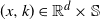 $(x,k)\in \mathbb{R}^d \times \mathbb{S}$
, there exist some positive constants c and C, independent of x, k, and
 $t_n$
, satisfying
 \begin{equation*} \sup_{\psi\leqslant 1+|\cdot|^{\kappa_1}}\{\bar{P}_{t_n}\psi(x,k)-\mu_{\gamma}(\psi)\} \leqslant C(1+|x|^{\kappa_1})\mathrm{e}^{-ct_n}, \end{equation*}
where the constant
 $\kappa_1$
is as in Assumption 1.2.
Under Assumption 1.2, the matrices
 $-Q_{c,\kappa_j}$
with
 $j=1,2$
are both nonsingular M-matrices with some constants
 $\kappa_1 \in (1,\alpha)$
and
 $\kappa_2\in (0,\kappa_1/4]$
; it follows from Lemma 2.1(iv) that there exist vectors
 $\xi^{(j)}=\big(\xi_1^{(j)},\ldots,\xi_N^{(j)}\big)\gg 0$
such that the vectors
 $\beta^{(j)} \, :\!= \, -Q_{c,\kappa_j} \xi^{(j)} \gg 0$
.
Letting
 $\bar{c}^{(j)} = \min_{i\in\mathbb{S}}\big\{{\beta_i^{(j)}}/{2\xi_i^{(j)}}\big\}$
, we know that
 $\bar{c}^{(j)}>0$
for
 $j=1,2$
. For the constants
 $\kappa_1 \in (1,\alpha)$
and
 $\kappa_2\in(0,\kappa_1/4]$
in Assumption 1.2, let the Lyapunov function be
 \begin{equation} V^{(j)}(x,i) = (1+|x|^2)^{\kappa_j/2}\xi_i^{(j)} = V^{(j)}(x) \xi_i^{(j)},\end{equation}
with
 $V^{(j)}(x)=(1+|x|^2)^{\kappa_j/2}$
and
 $j\in \{1,2\}$
.
Proof of Proposition
A.1. First, we show that the Lyapunov condition holds. For
 $V^{(j)}(x,i)$
in (A.1), using Taylor’s expansion and Young’s inequality, for any
 $\varepsilon>0$
there exists some positive constant
 $C(\varepsilon)$
such that
 \begin{align} & \int_{\mathbb{R}^d_0}\big[V^{(j)}(x+\sigma z,i)-V^{(j)}(x,i) - \langle\nabla V^{(j)}(x,i),\sigma z\rangle\mathbf{1}_{\{|z|\leqslant 1\}}\big] \frac{d_{\alpha}}{|z|^{d+\alpha}}\,\mathrm{d}z \nonumber \\ & \qquad = \int_{|z|>1}[V^{(j)}(x+\sigma z,i)-V^{(j)}(x,i)]\frac{d_{\alpha}}{|z|^{d+\alpha}}\,\mathrm{d}z \nonumber \\ & \qquad\quad + \int_{0<|z|\leqslant 1}\big[V^{(j)}(x+\sigma z,i)-V^{(j)}(x,i) - \langle\nabla V^{(j)}(x,i),\sigma z\rangle\mathbf{1}_{\{|z|\leqslant 1\}}\big] \frac{d_{\alpha}}{|z|^{d+\alpha}}\,\mathrm{d}z \nonumber \\ & \qquad \leqslant \frac{d_{\alpha}\kappa_j(3-\kappa_j)\sqrt{d}\sigma_{d-1}}{2(2-\alpha)}\xi_i^{(j)} + d_{\alpha}\kappa_j\sigma_{d-1}\bigg(\frac{|x|^{\kappa_j-1}}{\alpha-1} + \frac{1}{\alpha-\kappa_j}\bigg)\xi_i^{(j)} \nonumber \\ & \qquad \leqslant \varepsilon V^{(j)}(x,i) + C(\varepsilon), \end{align}
where
 $\sigma_{d-1}=2\pi^{{d}/{2}}/\Gamma({d}/{2})$
. In addition, under Assumption 1.1 and using Young’s inequality, for any
 $\varepsilon>0$
there exists some positive constant
 $C(\varepsilon)$
such that
 \begin{align} & \langle g(x,i),\nabla V^{(j)}(x,i)\rangle \nonumber \\ & \quad = \kappa_j(1+|x|^2)^{\kappa_j/2-1}\xi_i^{(j)}\langle g(x,i)-g(0,i),x\rangle + \kappa_j(1+|x|^2)^{\kappa_j/2-1}\xi_i^{(j)}\langle g(0,i),x\rangle \nonumber \\ & \quad \leqslant \kappa_j(1+|x|^2)^{\kappa_j/2-1}\xi_i^{(j)}c_i|x|^2 + |g(0,i)|\kappa_j(1+|x|^2)^{\kappa_j/2-1}|x|\xi_i^{(j)} \nonumber \\ & \quad = \kappa_j(1+|x|^2)^{\kappa_j/2}\xi_i^{(j)}c_i - \kappa_j(1+|x|^2)^{\kappa_j/2-1}\xi_i^{(j)}c_i + |g(0,i)|\kappa_j(1+|x|^2)^{\kappa_j/2-1}|x|\xi_i^{(j)} \nonumber \\ & \quad \leqslant \kappa_j c_i V^{(j)}(x,i)+\varepsilon V^{(j)}(x,i) + C(\varepsilon). \end{align}
Combining (4.3), (A.2), and (A.3) yields
 \begin{align} \mathcal{A}V^{(j)}(x,i) & \leqslant \kappa_j c_i V^{(j)}(x,i)+QV^{(j)}(x,i)+2\varepsilon V^{(j)}(x,i) + 2C(\varepsilon) \nonumber \\ & \leqslant \big[(Q+\kappa_j\operatorname{diag}(c_1,\ldots,c_N))\xi^{(j)}\big]_iV^{(j)}(x) + 2\varepsilon V^{(j)}(x,i) + 2C(\varepsilon) \nonumber \\ & = -\beta_i^{(j)}V^{(j)}(x) + 2\varepsilon V^{(j)}(x,i) + 2C(\varepsilon) \nonumber \\ & \leqslant -\bar{c}^{(j)}V^{(j)}(x,i) + C, \end{align}
where the last inequality holds since
 $\varepsilon={\beta_i^{(j)}}/{4\xi_i^{(j)}}$
. This implies (see [Reference Gurvich11, Proof of Lemma 7.2]) that
 \begin{equation} \mathbb{E}V^{(j)}\big(X_t^{x,k},R_t^{k}\big) \leqslant \mathrm{e}^{-\bar{c}^{(j)}t}V^{(j)}(x,k) + C\big(1-\mathrm{e}^{-\bar{c}^{(j)}t}\big). \end{equation}
Second, the process
 $(X_t,R_t)_{t\geqslant 0}$
defined in (1.1) is strong Feller and irreducible, which can be obtained from the discussions in [Reference Xi35, Theorems 3.2 and 4.5], [Reference Yin and Zhu39, Theorem 2.24], and [Reference Xi37, Theorems 5.6 and 6.3]. Combining the above Lyapunov condition, strong Feller, and irreducibility, it follows from [Reference Meyn and Tweedie26, Theorem 6.1] or [Reference Xi35, Theorem 5.4] that the process
 $(X_t,R_t)_{t\geqslant 0}$
is exponentially ergodic with ergodic measure
 $\mu$
. Furthermore, there exist some positive constants c and C, both independent of x, k, and t, satisfying
 \begin{equation*} \sup_{\psi\leqslant 1+V^{(j)}}\{P_{t}\psi(x,k)-\mu(\psi)\} \leqslant C\big(1+V^{(j)}(x,k)\big)\mathrm{e}^{-ct}. \end{equation*}
Finally, we take expectations with respect to the ergodic measure
 $\mu$
on both sides of (A.5), and knowing that, for
 $t=1$
,
 $\mu(V^{(j)}) \leqslant \mathrm{e}^{-\bar{c}^{(j)}}\mu(V^{(j)})+C$
, this implies that
 $\mu(V^{(j)})\leqslant C$
for some constant
 $C>0$
. The proof is complete.
Proof of Proposition
A.2. Let
 $V^{(1)}$
be as defined in (A.1). It follows from Lemma A.1 that
 \begin{equation*} \mathcal{A}_{\gamma}V^{(1)}(x,k) = \gamma\mathcal{A}V^{(1)}(x,k) + \mathcal{R}_{V^{(1)},1} + \mathcal{R}_{V^{(1)},2} + \mathcal{R}_{V^{(1)},3} + \mathcal{R}_{V^{(1)},4}, \end{equation*}
where
 \begin{align*} \mathcal{R}_{V^{(1)},1} & = (\mathrm{e}^{\gamma Q}-\mathrm{I}_d-\gamma Q)V^{(1)}(x,k), \\ \mathcal{R}_{V^{(1)},2} & = (\mathrm{e}^{\gamma Q}-\mathrm{I}_d)\mathbb{E}\big[V^{(1)}\big(Y_{\gamma}^{x,k},k\big)-V^{(1)}(x,k)\big], \\ \mathcal{R}_{V^{(1)},3} & = \int_0^1\langle\nabla V^{(1)}(x+r\gamma g(x,k),k)-\nabla V^{(1)}(x,k),\gamma g(x,k)\rangle\,\mathrm{d}r, \\ \mathcal{R}_{V^{(1)},4} & = \mathbb{E}\int_0^\gamma[\mathcal{J}V^{(1)}(x+\gamma g(x,k)+\sigma Z_s,k) - \mathcal{J}V^{(1)}(x,k)]\,\mathrm{d}s \end{align*}
and
 \begin{equation*} \mathbb{E}\big[V^{(1)}\big(Y_{\gamma}^{x,k},k\big)-V^{(1)}(x,k)\big] = \gamma\mathcal{J}V^{(1)}(x,k) + \gamma\langle\nabla V^{(1)}(x,k),g(x,k)\rangle + \mathcal{R}_{V^{(1)},3} + \mathcal{R}_{V^{(1)},4}. \end{equation*}
We need to give estimates for the remainders
 $\mathcal{R}_{V^{(1)},i}$
,
 $i=1,2,3,4$
.
For the term
 $\mathcal{R}_{V^{(1)},1}$
and for small enough
 $\gamma>0$
, we know that
 \begin{equation} |\mathcal{R}_{V^{(1)},1}| \leqslant C\gamma^2V^{(1)}(x,k). \end{equation}
For
 $\kappa_1 \in (1,\alpha)$
in Assumption 1.2 and using the interpolation inequality in [Reference Krylov17, Theorem 3.2.1], we know that, for any
 $x\in \mathbb{R}^d$
,
 \begin{equation*} [\nabla V]_{\kappa_1-1;B_1(x)} \leqslant C\varepsilon^{1-\kappa_1}[V^{(1)}]_{1;B_1(x)} + C\varepsilon^{2-\kappa}\|\nabla^2 V^{(1)}\|_{\infty}, \end{equation*}
where
 $B_1(x)=\{z\colon|z-x|\leqslant 1\}$
. Taking
 $\varepsilon=1+|x|$
, we have
 $[\nabla V^{(1)}]_{\kappa_1-1;\mathbb{R}^d} \leqslant C$
, so
 \begin{align} |\mathcal{R}_{V^{(1)},3}| & = \bigg|\int_0^1\bigg\langle \frac{\nabla V^{(1)}(x+r\gamma g(x,k),k)-\nabla V^{(1)}(x,k)}{|r\gamma g(x,k)|^{\kappa_1-1}} |r\gamma g(x,k)|^{\kappa_1-1}, \gamma g(x,k)\bigg\rangle\,\mathrm{d}r\bigg| \nonumber \\ & \leqslant C|\gamma g(x,k)|^{\kappa_1} \leqslant C\gamma^{\kappa_1} V^{(1)}(x,k). \end{align}
Since
 \begin{equation*} \mathcal{R}_{V^{(1)},4} = \mathbb{E}\int_0^\gamma \frac{\mathcal{J}V^{(1)}(x+\gamma g(x,k)+\sigma Z_{s},k)-\mathcal{J}V^{(1)}(x,k)} {|\gamma g(x,k)+\sigma Z_s|^{2-\alpha}}|\gamma g(x,k)+\sigma Z_s|^{2-\alpha}\,\mathrm{d}s, \end{equation*}
for small enough
 $\gamma>0$
we have
 \begin{equation} |\mathcal{R}_{V^{(1)},4}| \leqslant C(1+|x|^{2-\alpha})\gamma^{{2}/{\alpha}} \leqslant C\gamma^{{2}/{\alpha}}V^{(1)}(x,k), \end{equation}
where the second inequality holds from [Reference Chen, Jin, Xiao and Xu7, Lemma 3.1] and the fact that
 $3-\alpha>{2}/{\alpha}$
for
 $\alpha \in (1,2)$
.
Since
 \begin{align*} \mathcal{R}_{V^{(1)},2} & = (\mathrm{e}^{\gamma Q}-\mathrm{I}_d)\mathbb{E}\big[V^{(1)}\big(Y_{\gamma}^{x,k},k\big)-V^{(1)}(x,k)\big] \\ & = (\mathrm{e}^{\gamma Q}-\mathrm{I}_d)\mathbb{E}\{\gamma\mathcal{J}V^{(1)}(x,k) + \gamma\langle\nabla V^{(1)}(x,k),g(x,k)\rangle + \mathcal{R}_{V^{(1)},3} + \mathcal{R}_{V^{(1)},4}\}, \end{align*}
it follows from (A.2) and the estimates for
 $|\mathcal{R}_{V^{(1)},3}|$
and
 $|\mathcal{R}_{V^{(1)},4}|$
that, for small enough
 $\gamma>0$
,
 \begin{align} |\mathcal{R}_{V^{(1)},2}| & \leqslant C\gamma\{\gamma[\varepsilon V^{(1)}(x,k)+C(\varepsilon)] + \gamma V^{(1)}(x,k) + \gamma^{\kappa_1}V^{(1)}(x,k) + \gamma^{{2}/{\alpha}}V^{(1)}(x,k)\} \nonumber \\ & \leqslant C\gamma^2 V^{(1)}(x,k) + C\gamma^2. \end{align}
Combining (A.6), (A.7), (A.8), and (A.9), for small enough
 $\gamma>0$
we know that
 \begin{align*} |(\mathcal{A}_{\gamma} - \gamma\mathcal{A})V^{(1)}(x,k)| & \leqslant |\mathcal{R}_{V^{(1)},1}| + |\mathcal{R}_{V^{(1)},2}| + |\mathcal{R}_{V^{(1)},3}| + |\mathcal{R}_{V^{(1)},4}| \\ & \leqslant C(\gamma^2+\gamma^{\kappa_1} + \gamma^{{2}/{\alpha}}) V^{(1)}(x,k)+C\gamma^2, \end{align*}
and thus
 $|(\mathcal{A}_{\gamma} - \gamma\mathcal{A})V^{(1)}(x,k)| \leqslant C\gamma^{\kappa_1\wedge{2}/{\alpha}}V^{(1)}(x,k) + C\gamma^2$
. It then follows from (A.5) that
 \begin{align*} \mathbb{E}V^{(1)}\big(Y_{t_{n-1},t_{n}}^{x,k},R_{t_{n-1},t_{n}}^k\big) & = \mathbb{E}\big[V^{(1)}\big(Y_{t_{n-1},t_{n}}^{x,k},R_{t_{n-1},t_{n}}^k\big) - V^{(1)}(x,k)\big] + V^{(1)}(x,k) \\ & = \mathbb{E}\mathcal{A}_{\gamma}V^{(1)}(x,k) + V^{(1)}(x,k) \\ & \leqslant \mathbb{E}\big[\gamma\mathcal{A}V^{(1)}(x,k) + C\gamma^{\kappa_1\wedge{2}/{\alpha}}V^{(1)}(x,k) + C\gamma^2\big] + V^{(1)}(x,k) \\ & \leqslant (1-\bar{c}^{(1)}\gamma + C\gamma^{\kappa_1\wedge{2}/{\alpha}})V^{(1)}(x,k) + C\gamma. \end{align*}
Then, for small enough
 $\gamma>0$
, there exists some positive constant C, independent of n,
 $\gamma$
, x, and k, such that
 \begin{equation} \mathbb{E}V^{(1)}\big(Y_{t_{n}}^{x,k},R_{t_{n}}^k\big) \leqslant \bigg(1-\frac{\bar{c}^{(1)}}{2}\gamma\bigg)\mathbb{E}V^{(1)}\big(Y_{t_{n-1}}^{x,k},R_{t_{n-1}}^k\big)+C\gamma. \end{equation}
From standard discussions in [Reference Meyn and Tweedie25, Reference Meyn and Tweedie26], there exist some positive constants c and C such that
 \begin{equation*} \sup_{\psi \leqslant 1+V^{(1)}}\{\bar{P}_{t_n} \psi(x,k) -\mu_{\gamma}(\psi)\} \leqslant C(1+V^{(1)}(x))\mathrm{e}^{-ct_n}, \end{equation*}
which implies the desired result.
Proof of Lemma
A.1. For
 $\psi\in\mathcal{C}^2(\mathbb{R}^d,\mathbb{R}) \cap \mathcal{D}(\mathcal{A}) \cap \mathcal{D}(\mathcal{A}_{\gamma})$
, we have
 \begin{align} \mathcal{A}_{\gamma}\psi(x,k) & = \mathbb{E}\big[\psi\big(Y_{\gamma}^{x,k},R_{\gamma}^k\big)-\psi(x,k)\big] \nonumber \\ & = \mathbb{E}\big[\psi\big(Y_{\gamma}^{x,k},R_{\gamma}^k\big)-\psi\big(Y_{\gamma}^{x,k},k\big)\big] + \mathbb{E}[\psi\big(Y_{\gamma}^{x,k},k\big)-\psi(x,k)]. \end{align}
By the conditional expectation, it follows from [Reference Mao and Yuan23, Theorem 1.44] that
 \begin{align} & \mathbb{E}\big[\psi\big(Y_{\gamma}^{x,k},R_{\gamma}^k\big) - \psi\big(Y_{\gamma}^{x,k},k\big)\big] \nonumber \\ & \qquad = \mathbb{E}\big\{\mathbb{E}\big[\psi\big(Y_{\gamma}^{x,k},R_{\gamma}^k\big) - \psi\big(Y_{\gamma}^{x,k},k\big)\big] \mid \hat{\mathcal{F}}_{\gamma}\big\} \nonumber \\ & \qquad = (\mathrm{e}^{\gamma Q}-\mathrm{I}_d)\mathbb{E}\psi\big(Y_{\gamma}^{x,k},k\big) \nonumber \\ & \qquad = (\mathrm{e}^{\gamma Q}-\mathrm{I}_d)\psi(x,k) + (\mathrm{e}^{\gamma Q}-\mathrm{I}_d)\mathbb{E}\big[\psi\big(Y_{\gamma}^{x,k},k\big)-\psi(x,k)\big] \nonumber \\ & \qquad = \gamma Q\psi(x,k) + (\mathrm{e}^{\gamma Q}-\mathrm{I}_d-\gamma Q)\psi(x,k) + (\mathrm{e}^{\gamma Q}-\mathrm{I}_d)\mathbb{E}\big[\psi\big(Y_{\gamma}^{x,k},k\big)-\psi(x,k)\big] \nonumber \\ & \qquad = \gamma Q\psi(x,k) + \mathcal{R}_1 + \mathcal{R}_2, \end{align}
where
 $\hat{\mathcal{F}}_{\gamma}$
is the filtration generated by the
 $\alpha$
-stable process
 $(Z_t)_{t\geqslant 0}$
at time
 $t=\gamma$
. Using Itô’s formula and Taylor’s expansion, we obtain
 \begin{align} & \mathbb{E}\big[\psi\big(Y_{\gamma}^{x,k},k\big)-\psi(x,k)\big] \nonumber \\ & \qquad = \mathbb{E}[\psi(x+\gamma g(x,k)+\sigma Z_{\gamma},k) - \psi(x+\gamma g(x,k),k) + \psi(x+\gamma g(x,k),k)-\psi(x,k)] \nonumber \\ & \qquad = \mathbb{E}\int_0^{\gamma}\mathcal{J}\psi(x+\gamma g(x,k)+\sigma Z_s,k)\,\mathrm{d}s + \gamma\langle\nabla\psi(x,k),g(x,k)\rangle \nonumber \\ & \qquad\quad + \int_0^1\langle\nabla\psi(x+r\gamma g(x,k),k) - \nabla\psi(x,k),\gamma g(x,k)\rangle\,\mathrm{d}r \nonumber \\ & \qquad = \gamma\mathcal{J}\psi(x,k) + \mathbb{E}\int_0^{\gamma}[\mathcal{J}\psi(x+\gamma g(x,k)+\sigma Z_s,k) - \mathcal{J}\psi(x,k)]\,\mathrm{d}s \nonumber \\ & \qquad\quad + \gamma\langle\nabla\psi(x,k),g(x,k)\rangle + \mathcal{R}_3. \end{align}
Combining (4.3), (A.11), (A.12), and (A.13), we get the desired result.
A.2. Moment estimates
Moment estimates for the process
 $(X_t,R_t)_{t\geqslant 0}$
can be obtained from the Lyapunov condition in Appendix A.1. Combining this with the generator comparison in Lemma A.1 yields moment estimates for the EM scheme
 $(Y_{t_n},R_{t_n})_{n\in \mathbb{N}_0}$
.
Proof of Lemma 3.2.
-
(i) The moment estimate for the process
$(X_t^{x,k},R_t^{k})_{t\geqslant 0}$
holds from (A.5), i.e. for
$\kappa_1\in (1,\alpha)$
in Assumption 1.2, (A.14)which implies the desired estimate.
\begin{equation} \mathbb{E}|X_t^{x,k}|^{\kappa_1} \leqslant C\mathbb{E}V^{(1)}(X_t^{x,k},R_t^{k}) \leqslant C\mathrm{e}^{-\bar{c}^{(1)}t}V^{(1)}(x,k) + C(1-\mathrm{e}^{-\bar{c}^{(1)}t}), \end{equation}
-
(ii) By induction, it follows from (A.10) that there exists some positive constant C, independent of n, such that
\begin{equation*} \mathbb{E}V^{(1)}\big(Y_{t_{n}}^{x,k},R_{t_{n}}^k\big) \leqslant \bigg(1-\frac{\bar{c}}{2}\gamma\bigg)^n V^{(1)}(x,k) + C\gamma\sum_{j=1}^{n-1}\bigg(1-\frac{\bar{c}}{2}\gamma\bigg)^j \leqslant C(1+V^{(1)}(x,k)). \end{equation*}
-
(iii) Recall that
$X_t^{x,k} = x + \int_0^t g(X_s^{x,k},R_s^{k})\,\mathrm{d}s + \sigma Z_t$
, so for
$0\leqslant p\leqslant \kappa_1<\alpha$
, using the Hölder and Cramér–Rao inequalities, we get (A.15)where the inequality holds from the linear growth condition for g and the estimate for
\begin{equation} \mathbb{E}|X_t^{x,k}-x|^p = \mathbb{E}\bigg|\int_0^t g\big(X_s^{x,k},R_s^{k}\big)\,\mathrm{d}s + \sigma Z_t\bigg|^p \leqslant C(1+|x|^p)(t^{{p}/{\alpha}} \vee t^p), \end{equation}
$\mathbb{E}|X_t^{x,k}|^{\kappa_1}$
in (A.14).
-
(iv) Since
$X_{\gamma}^{x,k}-Y_{\gamma}^{x,k} = \int_{0}^{\gamma}[g(X_{s}^{x,k},R_{s}^k)-g(x,k)]\,\mathrm{d}s$
, using the Hölder inequality we get, for
$0\leqslant p\leqslant \kappa_1<\alpha$
, where the last inequality holds from the estimate for
\begin{align*} \mathbb{E}\big|X_{\gamma}^{x,k}-Y_{\gamma}^{x,k}\big|^p & = \mathbb{E}\bigg|\int_{0}^{\gamma}\big[g(X_{s}^{x,k},R_{s}^k)-g\big(x,R_{s}^k\big) + g\big(x,R_{s}^k\big)-g\big(x,k\big)\big]\, \mathrm{d}s\bigg|^p \\ & \leqslant C\mathbb{E}\bigg|\int_{0}^{\gamma}|X_{s}^{x,k}-x|\,\mathrm{d}s\bigg|^p + C(1+|x|^p)\mathbb{E}\bigg|\int_{0}^{\gamma}\mathbf{1}_{\{R_{s}^k\neq k\}}\,\mathrm{d}s\bigg|^p \\ & \leqslant C\gamma^{p-1}\int_{0}^{\gamma}\mathbb{E}|X_{s}^{x,k}-x|^p\,\mathrm{d}s + C(1+|x|^p)\gamma^{p-1}\int_{0}^{\gamma}\mathbb{P}(R_{s}^k \neq k)\,\mathrm{d}s \\ & \leqslant C(1+|x|^p)\gamma^{p(1+({1}/{\alpha}))}, \end{align*}
$\mathbb{E}|X_s^{x,k}-x|^p$
in (A.15) and the fact
$\mathbb{P}(R_{s}^k \neq k) \leqslant Cs$
with
$s\leqslant \gamma$
; indeed,
$\mathbb{P}(R_{s}^k \neq k)=1-\mathbb{P}(R_{s}^k=k)=1-(\mathrm{e}^{sQ})_{kk} \leqslant Cs$
for some small
$s\leqslant \gamma$
.
-
(v) Recalling that
$Y_{\gamma}^{x,k} = x + \gamma g(x,k)+\sigma Z_{\gamma}$
, it is obvious that for
$0 \leqslant p \leqslant \kappa_1<\alpha$
there exits some positive constant C such that
$\mathbb{E}|Y_{\gamma}^{x,k}-x|^p \leqslant C\gamma^{{p}/{\alpha}}(1+|x|^p)$
. The proof is complete.















Appendix B. One-step difference
Proof of Lemma
3.3. For
 $f\in \mathcal{C}^2(\mathbb{R}^d,\mathbb{R})$
satisfying
 $\|\nabla f\|_{\infty}+\|\nabla^2 f\|_{\infty}<\infty$
, we know that
 \begin{align} & (P_{\gamma}-\bar{P}_{\gamma})f(x,k) \nonumber \\ & \qquad = \mathbb{E}f\big(X_{\gamma}^{x,k},R_{\gamma}^k\big) - \mathbb{E}f\big(Y_{\gamma}^{x,k},R_{\gamma}^k\big) \nonumber \\ & \qquad = \mathbb{E}\big\langle\nabla f(x,k),X_{\gamma}^{x,k}-Y_{\gamma}^{x,k}\big\rangle + \mathbb{E}\big\langle\nabla f\big(x,R_{\gamma}^k\big) - \nabla f(x,k),X_{\gamma}^{x,k}-Y_{\gamma}^{x,k}\big\rangle \nonumber \\ & \qquad \quad + \mathbb{E}\int_0^1\big\langle\nabla f\big(Y_{\gamma}^{x,k} + r\big[X_{\gamma}^{x,k}-Y_{\gamma}^{x,k}\big], R_{\gamma}^k\big) - \nabla f\big(x,R_{\gamma}^k\big),X_{\gamma}^{x,k}-Y_{\gamma}^{x,k}\big\rangle\,\mathrm{d}r \nonumber \\ & \qquad = \mathrm{I} + \mathrm{II} + \mathrm{III}. \end{align}
We first give the estimate for I. Recall that
 \begin{equation} \mathbb{E}\big[X_{\gamma}^{x,k}-Y_{\gamma}^{x,k}\big] = \int_{0}^{\gamma}\mathbb{E}\big[g\big(X_{s}^{x,k},R_{s}^{k}\big)-g(x,k)\big]\,\mathrm{d}s = \int_{0}^{\gamma}\int_{0}^s\mathbb{E}\mathcal{A}g\big(X_{u}^{x,k},R_{u}^{k}\big)\,\mathrm{d}u\,\mathrm{d}s, \end{equation}
where
 $\mathcal{A}$
is defined in (4.3). Under Assumption 1.1(ii), we claim that
 \begin{equation} |\mathcal{A}g(x,k)| \leqslant C(1+|x|), \end{equation}
which implies that
 \begin{equation*} \big|\mathbb{E}\big[X_{\gamma}^{x,k}-Y_{\gamma}^{x,k}\big]\big| \leqslant C\int_{0}^{\gamma}\int_{0}^s\mathbb{E}\big(1+|X_{u}^{x,k}|\big)\,\mathrm{d}u\,\mathrm{d}s \leqslant C(1+|x|)\gamma^2, \end{equation*}
where the moment estimate for
 $\mathbb{E}|X_{u}^{x,k}|$
is from Lemma 3.2. This yields that
 \begin{equation} |\mathrm{I}| \leqslant C\|\nabla f\|_{\infty}(1+|x|)\gamma^2. \end{equation}
For the second term II, by the conditional expectation we know that
 \begin{align*} \mathbb{E}\big\langle\nabla f\big(x,R_{\gamma}^k\big)-\nabla f(x,k),X_{\gamma}^{x,k} &-Y_{\gamma}^{x,k}\big\rangle \\ &= \mathbb{E}\big\{\big\langle\nabla f\big(x,R_{\gamma}^k\big)-\nabla f(x,k), \mathbb{E}\big[X_{\gamma}^{x,k}-Y_{\gamma}^{x,k} \mid R_{\gamma}^k\big]\big\rangle\big\}; \end{align*}
it follows from (B.2) and the linear growth condition for g that
 \begin{equation*} \big|\mathbb{E}\big[X_{\gamma}^{x,k}-Y_{\gamma}^{x,k} \mid R_{\gamma}^k\big]\big| = \bigg|\int_{0}^{\gamma}C\mathbb{E}\big(1+\big|X_{s}^{x,k}\big|\big)\,\mathrm{d}s\bigg| \leqslant C(1+|x|)\gamma. \end{equation*}
In addition,
 $|\mathbb{E}[\nabla f(x,R_{\gamma}^k)-\nabla f(x,k)]| = |[\mathrm{e}^{\gamma Q}-\mathrm{I}_d]\nabla f(x,k)| \leqslant C\|\nabla f\|_{\infty}\gamma$
. Thus, we have
 \begin{equation} |\mathrm{II}| \leqslant C\|\nabla f\|_{\infty}(1+|x|)\gamma^2. \end{equation}
For the last term III, we know that
 \begin{align*} & \bigg|\mathbb{E}\int_0^1\big\langle\nabla f\big(Y_{\gamma}^{x,k}+r\big[X_{\gamma}^{x,k}-Y_{\gamma}^{x,k}\big], R_{\gamma}^k\big)-\nabla f\big(x,R_{\gamma}^k\big),X_{\gamma}^{x,k}-Y_{\gamma}^{x,k}\big\rangle\,\mathrm{d}r\bigg| \\ & \qquad \leqslant \mathbb{E}\int_0^1 \frac{\big|\nabla f\big(Y_{\gamma}^{x,k}+r\big[X_{\gamma}^{x,k}-Y_{\gamma}^{x,k}\big],R_{\gamma}^k\big) - \nabla f\big(x,R_{\gamma}^k\big)\big|} {\big|Y_{\gamma}^{x,k}-x+r\big[X_{\gamma}^{x,k}-Y_{\gamma}^{x,k}\big]\big|^{\kappa_1-1}} \\ & \quad\qquad \times \big(\big|Y_{\gamma}^{x,k}-x + r\big[X_{\gamma}^{x,k}-Y_{\gamma}^{x,k}\big]\big|^{\kappa_1-1}\big)\big|X_{\gamma}^{x,k}-Y_{\gamma}^{x,k}\big|\, \mathrm{d}r \\ & \qquad \leqslant C(\|\nabla f\|_{\infty} + \|\nabla^2 f\|_{\infty}) \mathbb{E}\big(\big|Y_{\gamma}^{x,k}-x\big|^{\kappa_1-1}\big|X_{\gamma}^{x,k}-Y_{\gamma}^{x,k}\big| + \big|X_{\gamma}^{x,k}-Y_{\gamma}^{x,k}\big|^{\kappa_1}\big), \end{align*}
where the last inequality holds from the fact that, for any
 $x,y \in \mathbb{R}^d$
,
 $k\in \mathbb{S}$
, and
 $\tau \in (0,1)$
,
 \begin{equation*} |\nabla f(x,k)-\nabla f(y,k)| \leqslant C(\|\nabla f\|_{\infty}+\|\nabla^2 f \|_{\infty})|x-y|^{\tau}. \end{equation*}
By the Hölder inequality, we obtain
 \begin{align*} \mathbb{E}\big[\big|Y_{\gamma}^{x,k}-x\big|^{\kappa_1-1}\big|X_{\gamma}^{x,k}-Y_{\gamma}^{x,k}\big|\big] & \leqslant \big[\mathbb{E}\big|Y_{\gamma}^{x,k}-x\big|^{p(\kappa_1-1)}\big]^{{1}/{p}} \big[\mathbb{E}\big|X_{\gamma}^{x,k}-Y_{\gamma}^{x,k}\big|^q\big]^{{1}/{q}} \\ & \leqslant C(1+|x|^{\kappa_1})\gamma^{1+({\kappa_1}/{\alpha})}, \end{align*}
where
 \begin{align*}p=\frac{1}{2}\bigg(\frac{\alpha}{\alpha-1}+\frac{\alpha}{\kappa_1-1}\bigg). \end{align*}
This implies that
 \begin{equation} |\mathrm{III}| \leqslant C(\|\nabla f\|_{\infty} + \|\nabla^2 f\|_{\infty}) (1+|x|^{\kappa_1})\gamma^{1+({\kappa_1}/{\alpha})}. \end{equation}
The desired inequality holds from (B.1), (B.4), (B.5), and (B.6).
It remains to show the claim (B.3). Recall that
 \begin{align} \mathcal{A}g(x,k) & = \langle\nabla g(x,k),g(x,k)\rangle + Qg(x,k) + \int_{|z|>1}[g(x+\sigma z,k)-g(x,k)]\frac{d_{\alpha}}{|z|^{d+\alpha}}\,\mathrm{d}z \nonumber \\ & \quad + \int_{0<|z|\leqslant 1}[g(x+\sigma z,k)-g(x,k)-\langle\nabla g(x,k),\sigma z\rangle] \frac{d_{\alpha}}{|z|^{d+\alpha}}\,\mathrm{d}z. \end{align}
Since
 $\|\nabla g\|_{\infty} \leqslant C$
, we know that g satisfies the linear growth condition and
 \begin{equation} |\langle \nabla g(x,k), g(x,k) \rangle + Qg(x,k)| \leqslant C(1+|x|). \end{equation}
In addition, under
 $\|\nabla g\|_{\infty} +\|\nabla^2 g\|_{\infty}\leqslant C$
, by the Taylor expansion,
 \begin{equation*} \int_{|z|>1}[g(x+\sigma z,k)-g(x,k)]\frac{d_{\alpha}}{|z|^{d+\alpha}}\,\mathrm{d}z = \int_{|z|>1}\int_0^1\langle\sigma z,\nabla g(x+r\sigma z,k)\rangle\,\mathrm{d}r \frac{d_{\alpha}}{|z|^{d+\alpha}}\,\mathrm{d}z \end{equation*}
and
 \begin{multline*} \int_{0<|z|\leqslant 1}[g(x+\sigma z,k)-g(x,k)-\langle\nabla g(x,k),\sigma z\rangle] \frac{d_{\alpha}}{|z|^{d+\alpha}}\,\mathrm{d}z \\ = \int_{0<|z|\leqslant 1}\int_0^1\int_0^1\langle r\sigma z(\sigma z)^*, \nabla^2 g(x+\tilde{r}r\sigma z,k)\rangle_\mathrm{HS}\,\mathrm{d}\tilde{r}\,\mathrm{d}r \frac{d_{\alpha}}{|z|^{d+\alpha}}\,\mathrm{d}z. \end{multline*}
This implies that
 \begin{align*} \bigg|\int_{|z|>1}[g(x+\sigma z,k)-g(x,k)]\frac{d_{\alpha}}{|z|^{d+\alpha}}\,\mathrm{d}z\bigg| & \leqslant C, \\ \bigg|\int_{0<|z|\leqslant 1}[g(x+\sigma z,k)-g(x,k)-\langle\nabla g(x,k),\sigma z\rangle] \frac{d_{\alpha}}{|z|^{d+\alpha}}\,\mathrm{d}z\bigg| & \leqslant C. \end{align*}
Combining these with (B.7) and (B.8), the claim in (B.3) holds. The proof is complete.
Appendix C. Regularities for Stein’s equation
Letting
 $(X_0, R_0)=(x,k)$
, the Jacobi flow of
 $X_t$
along the direction
 $u \in \mathbb{R}^d$
is defined as
 \begin{equation*} \nabla_{u} X^{x,k}_{t} = \lim_{\varepsilon\rightarrow0}\frac{X^{x+\varepsilon u,k}_t - X^{x,k}_t}{\varepsilon}, \quad t \geqslant 0.\end{equation*}
Lemma C.1. Under Assumptions 1.1 and 1.2, with
 $\eta>0$
defined in (1.4), for
 $u_1,u_2 \in \mathbb{R}^d$
satisfying
 $|u_1|=|u_2|=1$
and
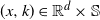 $(x,k)\in \mathbb{R}^d \times \mathbb{S}$
, there exists some positive constant C, independent of x, k, and t, such that
 $\mathbb{E}|\nabla_{u_1}X^{x,k}_t|^{4} \leqslant C\exp(\! -\eta t)$
and
 $\mathbb{E}|\nabla_{u_2}\nabla_{u_1}X^{x,k}_t|^2 \leqslant C\exp(\! -\eta t/4)$
.
The proof of Lemma C.1 is deferred to the end of this section.
Proof of Lemma
3.1. For any
 $u_1 \in \mathbb{R}^d$
satisfying
 $|u_1|=1$
,
 \begin{equation*} \nabla_{u_1}P_{t}h(x,k) = \nabla_{u_1}\mathbb{E}h\big(X_t^{x,k},R_t^{k}\big) = \mathbb{E}\big[\nabla h\big(X_t^{x,k},R_t^{k}\big)\nabla_{u_1}X_t^{x,k}\big]. \end{equation*}
Then, using Lemma C.1 and
 $\|\nabla h\|_{\infty}<\infty$
, there exists some positive constant C, independent of t, x, and k, such that
 \begin{align*} \|\nabla P_{t}h(x,k)\|_{\infty} & = \sup_{(x,k)\in\mathbb{R}^d\times\mathbb{S}}|\nabla_{u_1}P_{t}h(x,k)| \\ & \leqslant \|\nabla h\|_{\infty}\sup_{(x,k)\in\mathbb{R}^d\times\mathbb{S}}\mathbb{E}[|\nabla_{u_1}X_t^{x,k}|] \leqslant C\mathrm{e}^{-{\eta t}/{4}}. \end{align*}
For any
 $u_i \in \mathbb{R}^d$
with
 $i=1,2$
satisfying
 $|u_1|=|u_2|=1$
, we know that
 \begin{equation*} \nabla_{u_2}\nabla_{u_1}P_{t}h(x,k) = \mathbb{E}\big[\nabla h\big(X_t^{x,k},R_t^{k}\big)\nabla_{u_2}\nabla_{u_1}X_t^{x,k} + \nabla^2 h\big(X_t^{x,k},R_t^{k}\big)\nabla_{u_2}X_t^{x,k}\nabla_{u_1}X_t^{x,k}\big]. \end{equation*}
Using Lemma C.1 and
 $\|\nabla^i h\|_{\infty}<\infty$
with
 $i=1,2$
, there then exists some positive constant C, independent of t, x, and k, such that
 $|\nabla_{u_2}\nabla_{u_1}P_{t}h(x,k)| \leqslant C\mathrm{e}^{-{\eta t}/{8}}$
, which implies the estimate for
 $\|\nabla^2 P_{t}h(x,k)\|_{\infty}$
. The proof is complete.
Proof of Lemma
4.1. With arguments similar to [Reference Jin, Shen and Su14, Proposition 3.2], the solution
 $f_h$
of the Stein equation (4.5) can be expressed as
 $f_h(x,k) = -\int_{0}^{+\infty}[P_t h(x,k) -\mu(h)]\,\mathrm{d}t$
, where
 $P_t$
is the semigroup of the process
 $(X_t,R_t)_{t\geqslant 0}$
.
By the exponential ergodicity of the process
 $(X_t,R_t)_{t\geqslant 0}$
in Proposition A.1, there exists some positive constant C such that
 \begin{equation*} |f_h(x,k)| \leqslant \int_{0}^{+\infty}|P_t h(x,k)-\mu(h)|\,\mathrm{d}t \leqslant C(1+|x|^{\kappa_2}). \end{equation*}
For any
 $u_1\in \mathbb{R}^d$
, we know that
 \begin{equation*} \nabla_{u_1}f_h(x,k) = -\int_{0}^{+\infty}\nabla_{u_1}\mathbb{E}h\big(X_t^{x,k},R_t^k\big)\,\mathrm{d}t = -\int_{0}^{+\infty}\mathbb{E}\big[\nabla h\big(X_t^{x,k},R_t^k\big)\nabla_{u_1}X_t^{x,k}\big]\,\mathrm{d}t. \end{equation*}
Combining this with Lemma C.1 and the fact that
 $\|\nabla h\|_{\infty} \leqslant C$
, we get that
 $\|\nabla f_h(x,k)\|_{\infty} \leqslant C$
. The proof is complete.
Proof of Lemma
C.1. For any
 $u_1\in \mathbb{R}^d$
with
 $|u_1|=1$
, we have
 $\nabla_{u_1} X_0^{x,k}=u_1$
and
 \begin{equation*} \mathrm{d}\nabla_{u_1}X_t^{x,k} = \nabla g\big(X_t^{x,k},R_t^{k}\big)\nabla_{u_1}X_t^{x,k}\,\mathrm{d}t, \end{equation*}
which implies that
 \begin{equation*} \mathrm{d}|\nabla_{u_1}X_t^{x,k}|^{4} = \langle 4\nabla_{u_1}X_t^{x,k}|\nabla_{u_1}X_t^{x,k}|^{2}, \nabla g(X_t^{x,k},R_t^{x})\nabla_{u_1}X_t^{x,k}\rangle\,\mathrm{d}t \leqslant 4c_{R_t^{k}}|\nabla_{u_1}X_t^{x,k}|^{4}\,\mathrm{d}t, \end{equation*}
where the last inequality holds from (1.2). This can be estimated as
 \begin{equation} |\nabla_{u_1}X_t^{x,k}|^{4} \leqslant \exp\bigg(\int_0^t4c_{R_u^{k}}\,\mathrm{d}u\bigg), \end{equation}
and it follows from Lemma 1.1 that
 $\mathbb{E}|\nabla_{u_1}X_t^{x,k}|^{4} \leqslant C\exp(\! -\eta t)$
.
For any
 $u_1,u_2 \in \mathbb{R}^d$
with
 $|u_1|=|u_2|=1$
, we know that
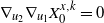 $\nabla_{u_2}\nabla_{u_1}X_0^{x,k}=0$
and
 \begin{equation*} \mathrm{d}\nabla_{u_2}\nabla_{u_1}X_t^{x,k} = \nabla g\big(X_t^{x,k},R_t^{k}\big)\nabla_{u_2}\nabla_{u_1}X_t^{x,k}\,\mathrm{d}t + \nabla^2g\big(X_t^{x,k},R_t^{k}\big)\nabla_{u_2}X_t^{x,k}\nabla_{u_1}X_t^{x,k}\,\mathrm{d}t. \end{equation*}
using Itô’s formula and Young’s inequality, for any
 $a>0$
we have
 \begin{align*} \mathrm{d}|\nabla_{u_2}\nabla_{u_1}X_t^{x,k}|^2 & = \big\langle2\nabla_{u_2}\nabla_{u_1}X_t^{x,k},\nabla g\big(X_t^{x,k},R_t^{k}\big)\nabla_{u_2}\nabla_{u_1}X_t^{x,k} \\ & \quad + \nabla^2g\big(X_t^{x,k},R_t^{k}\big)\nabla_{u_2}X_t^{x,k}\nabla_{u_1}X_t^{x,k}\big\rangle\,\mathrm{d}t \\ & \leqslant (2c_{R_t^{k}}+a)|\nabla_{u_2}\nabla_{u_1}X_t^{x,k}|^2\,\mathrm{d}t + C|\nabla_{u_2}X_t^{x,k}|^2|\nabla_{u_1}X_t^{x,k}|^2\,\mathrm{d}t, \end{align*}
which can be estimated as
 \begin{equation*} |\nabla_{u_2}\nabla_{u_1}X_t^{x,k}|^2 \leqslant C\int_0^t\exp\bigg(\int_s^t[2c_{R_u^{k}}+a]\,\mathrm{d}u\bigg) |\nabla_{u_2}X_s^{x,k}|^2|\nabla_{u_1}X_s^{x,k}|^2\,\mathrm{d}s. \end{equation*}
Combining this with (C.1), we know that
 \begin{align*} |\nabla_{u_2}\nabla_{u_1}X_t^{x,k}|^2 & \leqslant C\int_0^t\exp\bigg(\int_s^t[2c_{R_u^{k}}+a]\,\mathrm{d}u\bigg) \exp\bigg(\int_0^s4c_{R_u^{k}}\,\mathrm{d}u\bigg)\,\mathrm{d}s \\ & = C\int_0^t\mathrm{e}^{a(t-s)}\exp\bigg(\int_0^t2c_{R_u^{k}}\,\mathrm{d}u\bigg) \exp\bigg(\int_0^s2c_{R_u^{k}}\,\mathrm{d}u\bigg)\,\mathrm{d}s, \end{align*}
which implies that
 \begin{align*} \mathbb{E}|\nabla_{u_2}\nabla_{u_1}X_t^{x,k}|^2 & \leqslant C\int_0^t\mathrm{e}^{a(t-s)}\bigg[ \mathbb{E}\exp\bigg(\int_0^t4c_{R_u^{k}}\,\mathrm{d}u\bigg)\bigg]^{1/2} \bigg[\mathbb{E}\exp\bigg(\int_0^s4c_{R_u^{k}}\,\mathrm{d}u\bigg)\bigg]^{1/2}\,\mathrm{d}s \\ & \leqslant C\int_0^t\mathrm{e}^{a(t-s)}\exp\bigg({-}\frac{\eta}{2}t\bigg) \exp\bigg({-}\frac{\eta}{2}s\bigg)\,\mathrm{d}s \leqslant C\mathrm{e}^{-{\eta t}/{4}}, \end{align*}
where the second inequality holds from Lemma 1.1 and the last inequality holds by
 $a=\eta/4$
. The proof is complete.
Acknowledgements
We wish to thank the editors and referees for their helpful comments.
Funding Information
X. Jin is supported by the National Natural Science Foundation of China (grant no. 12401176), and the Fundamental Research Funds for the Central Universities (grant no. JZ2025HGTB0178).
Competing Interests
There were no competing interests to declare which arose during the preparation or publication process of this article.



