I. INTRODUCTION
At the onset of a cone indentation contact, due to the tip acuity and its stress/strain concentration beneath the tip of indenter, the contact may cause a finite amount of plastic yield even at small-scale indentation loading. Accordingly, the plastic flow would play an important role not only in elastoplastic but also in viscoelastic-plastic cone indentation contact problems. In elastoplastic regime, the Meyer’s contact hardness H M is uniquely described in terms of the so-called plasticity index of E′tan β/Y that is defined as the indentation strain (tan β) divided by the strain at the elastic limit (Y/E′) using the elastic modulus E′ (= E/(1−ν 2); E is Young’s modulus and ν is Poisson’s ratio), inclined face angle β of a cone indenter, and the plastic yield stress Y.Reference Johnson1 The Meyer hardness H M equals H M (elastic) = E′tan β/2 in the elastic extreme of the plasticity index less than 1 and reaches H M (plastic) = C·Y (C: the constraint factor), when the index exceeds about 50, where the contact behavior becomes very plastic and ductile. Strain hardening (work hardening) adds a further complication to the elastoplastic contact problems, requiring the concept of the representative yield stress Y R at the representative strain ε R to uniquely describe the normalized hardness H M/Y R as a function of E′tan β/Y R.Reference Johnson1, Reference Tabor2 Such complication associated with strain-hardening makes it difficult to determine the yield stress Y from the contact hardness observed in experiments, though the elastic modulus E′ is successfully determined from the unloading stiffness S using the elastic approximation of 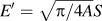 , if the projected contact area A is properly evaluated.Reference Oliver and Pharr3
A cone indenter pressed into contact with a viscoelastic body, such as an ordinary organic polymer, would cause the plastic yield along with the time-dependent viscoelastic deformation and flow. The irreversible deformation and flow associated with the simultaneous combination of plastic yield and viscous flow makes the contact problems crucially more complicated, leading to one of very intractable indentation contact problems. By way of example, the time (t) dependent stress relaxation function E′(t) is always as well as significantly underestimated, and the creep compliance function D′(t) is highly overestimated unless we properly eliminate the plastic yield from the indentation contact data.
The present authors have invented an instrumented indentation microscope that enables to make the in-situ measurement of indentation contact area (A) along with the indentation load (P) and the penetration depth (h), as reported in the literature.Reference Miyajima and Sakai4–Reference Hakiri, Matsuda and Sakai6 Using the indentation microscope, we can determine the contact hardness as well as the elastic modulus not only of bulk materials but also of coating/substrate composites without making any undesirable assumptions and approximations for estimating the indentation contact area. However, due to the fact that we have not been able to determine in experiments the indentation contact area A in the conventional instrumented indentation test systems, the current experimental works of indentation contact mechanics have always been conducted within the penetration-depth-based framework.
The major objective of this study is to propose the contact-area-based mechanics for a cone indentation contact, instead of the conventional penetration-depth-based analysis, to afford a sound theoretical basis to the experimental analysis for the instrumented indentation microscope. These theoretical considerations on elastoplastic as well as linear viscoelastic deformation and flow will be followed and supported with the numerical finite element analyses (FEA).
II. THEORETICAL CONSIDERATIONS
A. Indentation load P versus contact area A hysteresis relationship
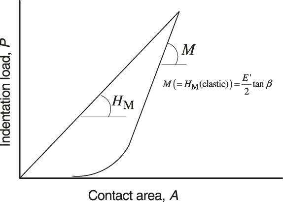
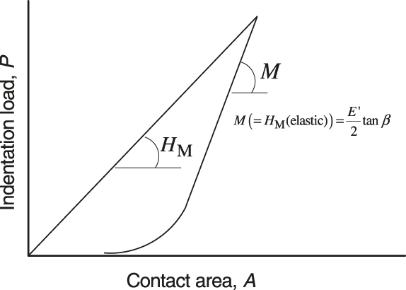
Due to the geometrical similarity of cone indentation contact, the Meyer hardness H M defined by the indentation load P divided by the projected contact area A, i.e., H M = P/A, is independent of the depth of penetration, namely independent of the contact area, if the indentation size effect is insignificant. This fact implies that the P–A relationship in its loading path will be linear with the slope of H M. Accordingly, the P–A loading relation measured on the instrumented indentation microscope directly yields H M without using any of approximations and assumptions, as schematically shown in Fig. 1.
Schematic of indentation load P versus contact area A diagram (P–A diagram).
The Sneddon’s elastic formula of the P–A relation for a conical indentation contact isReference Sneddon7
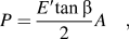
in terms of the elastic modulus E′ and the inclined face-angle β of the cone indenter. The Meyer hardness of the elastic body H M (elastic) as the mean contact pressure of P/A, therefore, is related to the elastic modulus, as follows;

In the conventional penetration-depth-based contact mechanics, since the contact deformation is well approximated to be purely elastic at the onset of unloading, one can successfully utilize the unloading stiffness S (= dP/dh) at the peak indentation load along the unloading P–h path to estimate E′ through the relation of
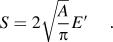
Let us consider the same unloading process in a P–A diagram like as in a P–h diagram. It is easy to show that the unloading modulus M defined by the slope of P–A unloading path, i.e., M = dP/dA at the peak indentation load (see Fig. 1), is readily related to S in the following formula;
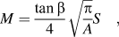
for conical indentation contact. Substituting Eq. (3) into Eq. (4) results in
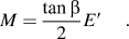
The unloading modulus M, therefore, equals the elastic Meyer hardness, H M (elastic) [Eq. (2)]. The fact of this coincidence between Eqs. (2) and (5) is a result of the elastic approximation included in Eq. (3) at the onset of indentation unloading, as schematically shown in Fig. 1. Accordingly, it will be practically significant that the experimentally observed P–A loading and unloading paths directly yield the Meyer hardness H M and the elastic modulus E′ from the respective linear slopes without any elastic approximations and assumptions that have always been required in the conventional P–h-based analysis to estimate the contact area A. This is the major reason why the present authors emphasize the scientific significances for inventing an instrumented indentation microscope and examining a contact-area-based indentation contact mechanics.
B. Elastoplastic contact area
Consider an elastoplastic body having the elastic modulus of E′ and the plastic yield stress Y. A conical indenter with the inclined face-angle of β is supposed to be pressed into contact with this elastoplastic body at an applied indentation load of P, resulting in the projected elastoplastic contact area of A. From the definition of the Meyer hardness H M, the contact area induced by the load P is simply given by

The contact area A includes all of the essential information on the elastic/plastic deformation.
Consider the indentation contact problem for an ideally elastic body with the elastic modulus of E′. This elastic body is equivalent to the above elastoplastic body with an infinite yield stress. The contact area A e of this elastic body under the given indentation load P is, therefore from Eq. (1), expressed byReference Johnson1, Reference Sneddon7

The contact area A e includes the elastic information of the body indented.
In contrast to this elastic extreme, in the plastic extreme of the present elastoplastic body with an infinite elastic modulus, i.e., a rigid-perfectly plastic body with the yield stress Y, the contact hardness is well related to the yield stress Y through the constraint factor C, as H M(= H M(plastic)) = C·Y, and then the plastic contact area A p of this rigid-perfectly plastic body can be given byReference Johnson1

for the given indentation load, P. The expression of Eq. (8) survives even for plastic bodies with strain hardening by replacing Y with its representative value of Y R.Reference Sakai, Akatsu, Numata and Matsuda8
It will be well expected that the elastoplastic contact area A will be reduced to the elastic contact area A e, i.e., A = A e, when the yield stress Y increases to infinity and/or the elastic modulus E′ decreases to a value small enough in its elastic extreme. In a similar way, A will meet A p, i.e., A = A p, in the plastic extreme with an infinite elastic modulus, and/or an infinitesimal yield stress. The most critical question in the present context: “Is the contact area A of an elastoplastic body with E′ and Y simply given by the sum of the elastic contact area A e of the perfectly elastic body with E′ and the plastic contact area A p of the purely plastic body with Y?” In other words, “Is the equality of

at a given indentation load P acceptable or not?” In fact, the relation given in Eq. (9) naturally yields A = A e in the perfectly elastic regime, where A p reduces to zero, while A = A p in the purely plastic extreme due to the diminishment of the elastic deformation, i.e., A e = 0.
The current theoretical/analytical framework of elastoplastic indentation contact mechanics, however, fails not only to give a proof for the validity of Eq. (9) but also to point out the scientific flaws included in this simple relationship of A = A e + A p. In the present work, therefore, to circumvent this difficulty, the authors utilized the numerical FEA results in the literature, the details of which have been reported in Ref. Reference Sakai, Akatsu, Numata and Matsuda8.
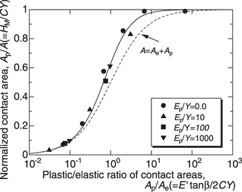
Figure 2 shows the FEA results (the several symbols with a best-fitted solid line) as their normalized plots of A p/A versus A p/A e. This best fitted solid line for the normalized plastic contact area A p/A is well described by the following semiempirical formula;
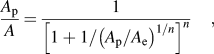
FEA results for the normalized plastic contact area, A p/A plotted against the plastic/elastic ratio of contact areas A p/A e, being equivalent to the Johnson’s hardness plot of H M/Y versus E′tan β/Y. The solid line is the semiempirical relation [Eq. (10) with n = 2/3]. The dashed line indicates the simple sum of A = A e + A p [Eqs. (9) and (11)].

in terms of the plastic/elastic ratio A p/A e of the contact areas and the empirically best-fitted exponent of n = 2/3. In contrast, the simple sum of Eq. (9) combined with Eqs. (6)–(8) leads to the following formula,
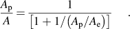
Accordingly, Eq. (10) with n = 1 straightforwardly results in Eq. (11). The dashed line in Fig. 2 indicates the relation of Eq. (11). As clearly seen in Fig. 2, the FEA results are always larger than the relation of A = A e + A p; meaning that the total contact area A is always smaller than the sum of the elastic and the plastic contact areas of A e + A p, i.e., A ≤ A e + A p. The principle of minimum energy requirement may well support this inequality, since the energy required to create the contact area A of the elastoplastic body with E′ and Y at a given indentation load of P must be less than the energies required to separately create the contact area A e of the purely elastic body with E′, and the contact area A p of the fully plastic body with Y, due to the elastic/plastic interaction that takes place in the elastoplastic body. The fact of the inequality, A ≤ A e + A p, defines the following correction factor, f, as the ratio of A to A e + A p:

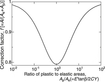
where the correction factor is always less than 1.0, i.e., f ≤ 1.0, and given by
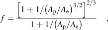
in terms of the ratio A p/A e. The correction factor f of Eq. (13) is plotted in Fig. 3 as a function of A p/A e, indicating that the correction factor f has a minimum value of about 0.8 at A p/A e = 1.0 and increasingly reaches to 1.0 both in the elastic contact of A p/A e ≪ 1.0 and the plastic contact of A p/A e ≫ 1.0. In other words, we need the largest correction for the simple sum of A = A e + A p, when the elastic contact deformation equals the plastic one, i.e., A e = A p.
The correction factor f(= A/(A e + A p)) as a function of the elastic/plastic ratio of contact areas A p/A e [see Eq. (13)].

The empirical fact of n = 2/3 for the FEA results suggests that, instead of the simple sum for the contact areas, A = A e + A p, the total volume of contact impression V at the indentation load P is well approximated by the simple sum of the impression volumes of V e and V p of the purely elastic and the purely plastic bodies, respectively, at the same indentation load P, i.e., V = V e + V p. Due to the geometrical similarity of cone/pyramid indentation, the volumetric sum of V = V e + V p readily results in A 3/2 = A e3/2 + A p3/2, and then straightforwardly leads to Eq. (10) with n = 2/3.
Once we notice the fact that Eqs. (6) and (8) result in

and the fact that Eqs. (7) and (8) lead to

we have an important finding that the FEA result plotted in Fig. 2 (the closed symbols with a best-fitted solid line) is an alternative expression for the so-called Johnson’s hardness plot of the normalized contact hardness H M/Y versus the plasticity index of E′tan β/Y.Reference Johnson1 Accordingly, in other words, the Johnson plot of H M/Y versus E′tan β/Y (i.e., H M/Y monotonically increases with the increase in E′tan β/Y and reaches the constraint factor of C in a fully ductile contact) indicates that the ratio of the plastic to the total contact areas A p/A(= H M/CY) monotonically increase from 0 to 1.0 with the increase in the plastic deformation of A p/A e(= E′tan β/2CY) from 0 (perfectly elastic) to infinity (fully ductile).
Once we know the elastic modulus E′ of the elastoplastic body from the unloading modulus M in the P–A diagram as demonstrated in Fig. 1 and then determine the elastic contact area A e using Eq. (7), therefore, it will be straightforward for us to determine the plastic contact area A p by utilizing Eqs. (7) and (12), as follows;
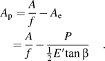
It should be noticed in Eq. (16) that the elastoplastic contact area A at the indentation load P must be observable prior to determining in experiment the plastic contact area A p. The constraint-factor-multiplied yield stress CY (or CY R) can then be determined through the formula of CY = P/A p, resulting in the Y-value by approximating C = 2.7 ∼ 3.0.Reference Sakai, Akatsu, Numata and Matsuda8
III. DETERMINATION OF THE LINEAR VISCOELASTIC FUNCTIONS THROUGH ELIMINATING PLASTIC DEFORMATION/FLOW IN CONE/PYRAMID INDENTATION CONTACTS
Consider a time-dependent mechanical behavior when a cone indenter is pressed into contact with a linear viscoelastic body. During the progressively growing penetration with time t, its contact area A ve(t) also grows, and the distribution of contact pressure changes with time, resulting in the time-dependent indentation load P(t). Using the principle of elastic-to-viscoelastic correspondence,Reference Shames and Cozzarelli9–Reference Sakai and Shimizu13 the Sneddon’s elastic solution of Eq. (1) is simply rewritten into the following hereditary integral in a linear viscoelastic regime through the replacement of the elastic modulus E′ with the stress relaxation function E′(t−t′) and the elastic contact area A(= A e) with the viscoelastic contact area A ve(t′);

An alternative of Eq. (17) is given in the following formula in terms of the creep compliance function, D′(t−t′);

where D′(t) is linked to E′(t) through the complementary relationship of 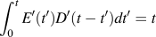 . Furthermore, the time-dependent Poisson’s ratio ν(t) has the relationship to E′(t) through
 in the Laplace space, where
 ,
 , and
 are, respectively, the Laplace transforms of the normal and shear relaxation moduli of E′(t) and G(t), and the viscoelastic Poisson’s ratio of ν(t). It is worthy of note that the Laplace transform of Eq. (17) leads to the Sneddon’s elastic formula [see Eq. (1)] in its Laplace-space, i.e.,
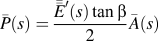 , in terms of the Carson’s modulus
 (the s-multiplied transform of E′(t)) defined by
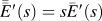 .Reference Shames and Cozzarelli9, Reference Roylance10
The most critical issue in viscoelastic-plastic contact problems for cone indentation is the plastic yield that may be induced beneath the tip of indenter. The time-dependent contact area A(t) includes not only the viscoelastic component A ve(t) but also the plastic one A p(t), resulting in A(t) > A ve(t). Accordingly, when we use Eqs. (17) and (18) in determining E′(t) and D′(t) by substituting the observed contact area A(t) into A ve(t), we always and significantly underestimate E′(t), and overestimate D′(t), indicating that the quantification of plastic yield is very essential in viscoelastic-plastic indentation contact problems.
The detailed procedures are summarized in what follows to properly eliminate the plastic contact area A p(t) from the observed contact area A(t) to yield the viscoelastic contact area A ve(t), and then to determine the viscoelastic functions.
A. The indentation load relaxation test under a stepwise contact area:
Consider a stepwise penetration at time t = 0 to keep a constant contact area of A 0 for t′ > 0 (this cannot be conducted in the conventional instrumented indentation apparatuses but can be done by the use of the instrumented indentation microscope).Reference Miyajima and Sakai4–Reference Hakiri, Matsuda and Sakai6 In this test, using the elastoplastic relation of A e = A/f − A p, the following viscoelastic contact area A ve(t) is simply given by

Equation (19) indicates that A ve(t′) is time-independent, for the plastic contact area A p(t′) has been fixed to the constant value of P(0)/(C·Y) for t′ ≥ 0 due to the load relaxation P(t) as well as the relaxation of mean contact pressure p m(t)(= P(t)/A 0), being always smaller than their initial values, i.e., P(t) ≤ P(0) and p m(t) ≤ p m(0).
Substituting the stepwise contact area of A ve(t′) = A ve(0)H(t′) into Eq. (17), we have the following formula for the stress relaxation function;
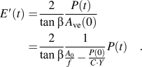
B. The indentation load relaxation test for a stepwise depth of penetration
In the conventional instrumented indentation tests, instead of applying a stepwise contact area to a specimen, we can apply a stepwise depth of penetration. In general, in this test configuration for a fixed depth of penetration, if the Poisson’s ratio is not 0.5, the contact area progressively increases with time during load relaxation.Reference Sakai14 Accordingly, we must rewrite Eq. (19) into
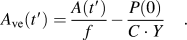
Substituting Eq. (21) into Eq. (17), and then making its Laplace transform, the Laplace-transformed stress relaxation function  is
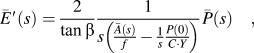
where s is the variable in the Laplace-space.  and
 are the Laplace transforms of A(t) and P(t), respectively. It is rather straightforward to obtain the stress relaxation function from the Laplace transform inversion of Eq. (22) in a numerical manner.
C. The indentation creep test for stepwise loading
A stepwise indentation loading of P(t′) = P 0H(t′) combined with Eq. (18) along with the relation of
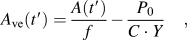
results in
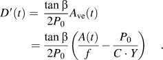
It must be noticed in Eq. (23) that the plastic contact area is assumed to be constant (P 0/(C·Y)) during the creep, for the creep deformation under a constant load of P 0 results in the contact stresses of P 0/A(t), that is always smaller than the initial contact stress of P 0/A(0) due to the growing contact area A(t) in creep deformation. Accordingly, no further postplastic yields is assumed to evolve for t > 0. This assumption will be acceptable to perfectly plastic and strain hardening materials. However, as addressed by Vanlandingham et al.,Reference Vanlandingham, Chang, Drzal, White and Chang15 due to the postplastic yield during the constant-load creeping of glassy polymers and strain-softening materials, the assumption of constant plastic yield (P 0/C·Y) in Eq. (23), in general, may allow an experimental uncertainty in determining the creep compliance function D′(t).
D. The indentation test for a constant rate of loading
Consider a load controlling penetration test with a constant rate of loading given by P(t′) = k Pt′ for t′ ≥ 0. Equation (18) combined with the following relationship,
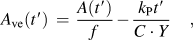
yields the following formula,
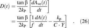
E. The indentation test for a constant rate of penetration
A constant rate of penetration with h(t′) = k ht′ for t′ ≥ 0 leads to a rather complicated contact behavior, where both of the load P(t) and the contact area A(t) are time-dependent, requiring the use of the Laplace-transform of Eq. (17), and then results in,
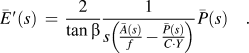
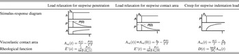
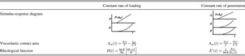
The Laplace-transform inversion of Eq. (27) finally yields the stress relaxation function of E′(t) in a numerical manner. The contact-area-based analyses discussed in this section are summarized in Tables I and II.
Viscoelastic stimulus- response diagrams and their constitutive equations.

 are the transformed E′(t), P(t), A ve(t).
Viscoelastic stimulus-response diagrams and their constitutive equations.

 are the transformed E′(t), P(t), A ve(t).
IV. FINITE ELEMENT STUDY ON THE VISCOELASTIC-PLASTIC CONTACT PROBLEMS
The theoretical considerations addressed in Section III are examined in this section through numerical FEA studies, where the inclined face-angle of the cone indenter is fixed to the Vickers–Berkovich-equivalent angle of 19.7° with the ANSYS code (Version 10.0).16 The contact friction is taken into account as the frictional coefficient ranging from 0.0 to 0.3.
A. Elastoplastic study
The elastoplastic FEA-models with the Von Mises criterion cover from purely elastic to fully ductile natures in the range of 1 ≤ E′/Y ≤ 1000 and the normalized coefficient of linear strain hardening of 0 ≤ E p/Y ≤ 1000, where the plastic hardening modulus E p is defined by σ = Y + E p·ε p at the stresses σ larger than Y for the plastic strains ε p. The conventional constitutive expression for linear strain hardening has been given by σ = Y + E Y(ε − Y/E) for σ ≥ Y in terms of the total strain ε using the modulus of linear hardening E Y. The strain hardening modulus E p, therefore, is related to E Y through the relation of 1/E p = 1/E Y − 1/E based on the incremental elastoplastic theory of dε = dε e + dε p, where ε e indicates the elastic strain.Reference Sakai, Akatsu, Numata and Matsuda8
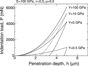
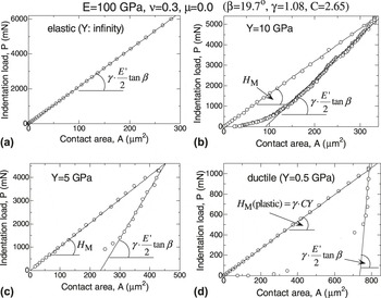
Examples of the P–h loading/unloading hysteresis relations are shown in Fig. 4, and their P–A hysteresis relations are given in Fig. 5. The P–A plots clearly indicate that the slope of the loading linear line yields the contact hardness, and the initial unloading modulus M directly represents the elastic hardness of M = (H M (elastic)) = γ(E′tan β/2), where the frontal factor γ = 1.08 (for ν = 0.3) is the correction factor reported by Hay et al.Reference Hay, Bolshakov and Pharr17 It should also be noticed that the loading slope H M of the very ductile model [Fig. 5(d); E = 100 GPa, Y = 0.5 GPa, E p = 0.0 GPa, ν = 0.3] coincides with its plastic value, H M (plastic) = γ·CY (γ = 1.08 and C = 2.65). Furthermore, the intensive examinations confirmed that the strain hardening and the contact friction have no effects on the unloading stiffness M. We can, therefore, determine in experiments the elastic modulus E′ from the unloading modulus M, even if strain hardening and/or contact friction is significant.
FEA results of the P–h loading/unloading hysteresis relations for the elastoplastic models having the Young’s modulus E = 100 GPa with various values of the yield stress Y.

FEA results of the P–A loading/unloading hysteresis relations for the elastoplastic models shown in Fig. 4.

B. Viscoelastic-plastic study
A simple viscoelastic–plastic body was examined; a viscous dashpot with the steady-state viscosity η is connected in series to an elastic-perfectly plastic component with the elastic modulus E′ and the yield stress Y, where the Von Mises criterion is assumed for plastic yielding. The material characteristics of η, E, Y, ν, and τ(= η/E′) are supposed to be 1.87 × 10¹³ Pa·s, 70 GPa, 5 GPa, 0.5, and 200 s, respectively. This set of material characteristics is rather close to that of a soda-lime silicate glass (SL-glass) at its glass-transition temperature, although the stress relaxation spectrum of SL-glass is more complicated.Reference Sakai and Shimizu13 The Poisson’s ratio is assumed to be 0.5 for simplicity, otherwise it becomes time-dependent during viscoelastic deformation and flow.Reference Roylance10, Reference Sakai14
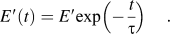
When the applied stress or the induced stresses σ are smaller than Y, i.e., σ < Y, the model is equivalent to the so-called Maxwell linear viscoelastic liquid, and its stress relaxation function E′(t) is given by
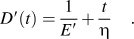
The creep compliance function D′(t) is, in a similar manner, expressed by
As mentioned in Section I, however, the cone indentation generates plastic deformation beneath the tip of indenter even at the onset of indentation contact. Accordingly, prior to determining the viscoelastic functions of E′(t) and D′(t), we must eliminate the plastic deformation from the indentation observables of P(t), A(t), h(t), etc. through the procedures demonstrated in Section III. In this section, two of the specific rheological tests are examined; (i) a stress relaxation test for a stepwise penetration of h(t′) = h 0H(t′) and (ii) a test for a constant rate of indentation loading of P(t′) = k P·t′.
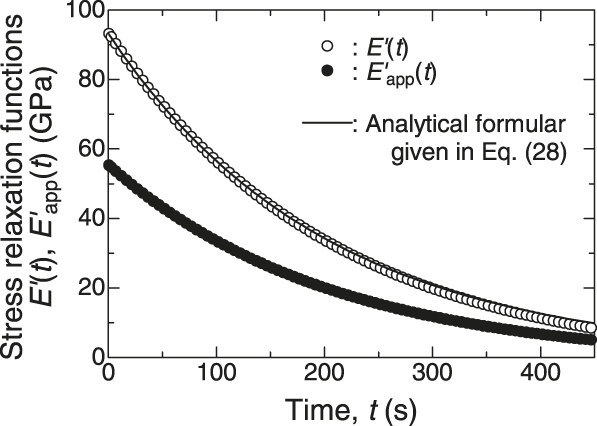
Figure 6 shows the numerical FEA results of the stress relaxation test under a stepwise penetration of h 0 = 5.0 μm for the stress relaxation functions of E′(t) (the open circles) calculated from the viscoelastic contact area of A ve(t), as well as the apparent modulus E′app(t) (the closed circles) determined by the use of the observed contact area A(t).
FEA results for the stress relaxation functions E′(t) calculated from the viscoelastic contact area A ve and the apparent modulus E′app(t) from the total contact area A. The significant discrepancy between E′(t) and E′app(t) is resulted from the plastic deformation and flow. The solid line indicates the analytical result of the present Maxwellian liquid [Eq. (28)].
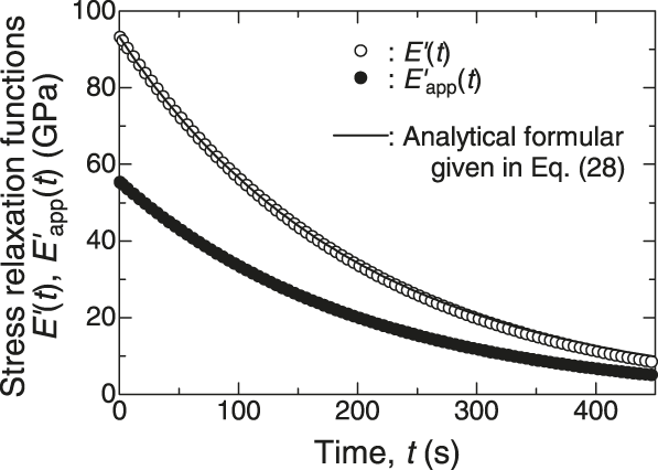
In the present numerical relaxation test, the contact area A(t) was always time-independent during the stress relaxation. Accordingly, the test is equivalent to the stepwise constant area test, and we can simply use Eq. (19) to eliminate the plastic deformation and then to determine the viscoelastic contact area of A ve. It should be noticed that this time-independent contact area is realized only for viscoelastic liquids with the Poisson’s ratio of 0.5 (incompressible liquids).Reference Sakai14 If the Poisson’s ratio is smaller than 0.5, it is actually time-dependent and monotonically increases to the value of 0.5 during the stress relaxation.Reference Roylance10, Reference Sakai14 This time-dependent Poisson’s effect, in turn, results in the time-dependent contact area of A(t) during the stress relaxation even under a fixed penetration of h 0, where we need to use Eqs. (21) and (22) to determine the stress relaxation function E′(t).
In Fig. 6, the stress relaxation modulus E′(t) was determined by the use of Eq. (20), whereas the apparent relaxation modulus, E′app(t), was calculated simply using the observed contact area A(t) that includes plastic deformation. As clearly seen in Fig. 6, the FEA-derived E′(t) satisfactory coincides with the analytical stress relaxation modulus [Eq. (28) with E′ = 93.3 GPa and τ = 200 s; the solid line in Fig. 6]. Figure 6 also clearly indicates a significant underestimate of the relaxation modulus whenever we neglect the plastic effect.
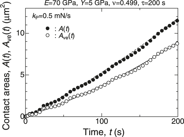
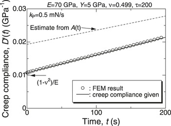
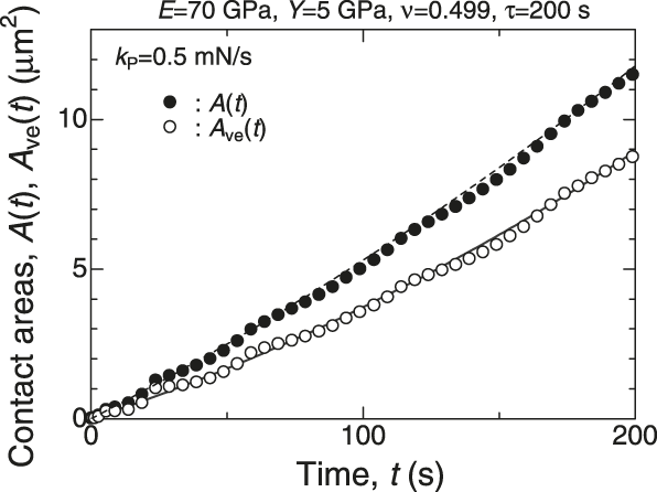
The FEA results for a constant rate of indentation loading with k p = 0.50 mN/s are shown in Fig. 7, where the growing contact areas A(t) (the closed circles) and A ve(t) (the open circles) are plotted against time t. We utilized Eq. (25) in determining the viscoelastic contact area A ve(t). Accordingly, in Fig. 7, the discrepancy between A(t) and A ve(t) indicates the amount of plastic deformation of k pt/C·Y. The creep compliance function D′(t) can then be calculated from the first-derivative of the area curve, dA ve(t)/dt, in Fig. 7 with Eq. (26), the result being plotted in Fig. 8 (the open circles). The solid line along the open circles indicates the analytical creep function of the FEA model [see Eq. (29) with E′ = 93.3 GPa and η = 1.87 × 10¹³ Pa·s]. The dashed line in Fig. 8 is the apparent creep curve estimated from the first derivative of the plastic-effect-included contact area A(t) (the closed circles in Fig. 7). As clearly shown in Fig. 8, when we neglect the plastic deformation, the creep compliance function is always as well as significantly overestimated.
FEA results for the evolutions of the contact areas in a constant-rate-of-loading test. Plastic yielding results in the progressively increasing discrepancy between A(t) (total contact area) and A ve(t) (viscoelastic contact area).
Creep compliance function D′(t) (the open circles) calculated from A ve(t) shown in Fig. 7. The solid line is the analytical relation of the present Maxwellian liquid [Eq. (29)]. The dashed line calculated from the total contact area A(t) always as well as significantly overestimates the compliance function due to the plastic deformation/flow.

V. CONCLUDING REMARKS
Nobody can determine the characteristic mechanical properties and functions in indentation tests, if the induced contact area A is unknown. The conventional instrumented indentation test systems, however, can only measure the induced penetration depth h. The indentation-induced contact profile may sink in or pile up that is dependent on the elastoplastic/viscoelastic nature of the material indented. Accordingly, in general, there is a crucial difficulty in estimating the contact area A from the penetration depth h.
The instrumented indentation microscope invented by the present authors can measure the in-situ contact area, leading to the way to the quantitative characterization of mechanical properties without any of undesirable assumptions and approximations associated with contact-area-estimate. In this article, the authors intensively discussed the contact-area-based indentation contact mechanics instead of the traditional penetration-depth-based analysis. In particular, the role of plasticity was examined in a quantitative manner in the elastoplastic indentation regime, and then the results were extended to the viscoelastic-plastic indentation contact problems.
In time-independent elastoplastic regime, the authors showed that the indentation load P versus contact area A relationship for a cone indentation is basically linear both for the loading and the unloading paths. The slope of the loading linear path directly yields the Meyer hardness H M, and the slope of the unloading line, i.e., the unloading modulus M, is related to the elastic modulus E′ through the relation of M = E′tan β/2, from which we can determine E′ in a precise manner without any of approximations and assumptions. To examine the contribution of the elastic deformation and the plastic flow to the total contact area A, the relationships of A to the purely elastic and the purely plastic contact areas of A e and A p were theoretically discussed and then demonstrated that the normalized relation between A p/A versus A p/A e is equivalent to the Johnson’s hardness plot of H M/Y versus E′tan β/Y.
In time-dependent linear viscoelastic regime, by extending the concept of A e and A p, a detailed discussion was made how to eliminate the plastic deformation/flow from the total contact area A(t) to yield the viscoelastic contact area A ve(t) prior to determining in experiments the linear viscoelastic parameters and functions.
FEA-based numerical studies were conducted not only in elastoplastic but also in viscoelastic-plastic regimes to confirm/support the theoretical considerations given in this work.
ACKNOWLEDGMENT
The authors acknowledge Dr. T. Miyajima (AIST, Japan) for his contributions to developing the instrumented indentation microscope.