1 Introduction
Ship internal wave wakes are commonly analysed by means of linear theory, assuming a source, pressure or thin-ship representation (Hudimac Reference Hudimac1961; Crapper Reference Crapper1967; Keller & Munk Reference Keller and Munk1970; Yih & Zhu Reference Yih and Zhu1989; Yeung & Ngyuen Reference Yeung and Ngyuen1999). The dead water resistance – the drag force due to the internal wave wake – on a semi-submerged slender prolate spheroid has been calculated assuming linear waves (Miloh & Tulin Reference Miloh and Tulin1989; Tulin & Miloh Reference Tulin and Miloh1991; Miloh, Tulin & Zilman Reference Miloh, Tulin and Zilman1993). The nonlinear internal wave wake in a two-layer fluid including the effect of the free surface due to a pressure distribution moving along the free surface was investigated by Parau, Vanden-Broeck & Cooker (Reference Parau, Vanden-Broeck and Cooker2007). Wave wake amplitudes, velocities and strain rates obtained from field measurements were found to compare poorly with the available linear prediction methods (Watson, Chapman & Apel Reference Watson, Chapman and Apel1992). Accurate evaluations of the internal ship wake are of interest from a detection point of view as well as for obtaining the dead water resistance. The wakes are also relevant for other purposes. Examples include the wave loads on infrastructures such as submerged floating tunnels, the construction of which is under consideration in fjords, inlets or coastal waters in Norway, Italy, Japan and China.
It seems that Tulin, Yao & Wang (Reference Tulin, Yao and Wang2000) provide the most updated calculations of the dead water wave wake, which they also compare with laboratory measurements. A direct comparison with their results is made in § 5.4. However, the ship model they used has a relative volume that is 10 times smaller compared with the observed ship described in our paper, where the pycnocline depth is the reference length. It is evident that the dead water cases investigated by Tulin et al. are well within the linear range, since nonlinear effects of interfacial elevations
 $\unicode[STIX]{x1D702}/h_{0}$
of a few per cent are small (where
 $\unicode[STIX]{x1D702}$
is the elevation and
 $h_{0}$
is the average depth of the pycnocline), while the interfacial excursions described in the present observations and calculations are indeed in the nonlinear range. A set of model scale experiments presented in Mercier, Vasseur & Dauxious (Reference Mercier, Vasseur and Dauxious2011), relevant to the special two-dimensional case, has emphasized the role of nonlinearity and non-stationarity in the dead water problem. In their experiments, the non-stationarity occurred in the subcritical range (Froude number
 $Fr<1$
), see their figure 11, while stationary conditions were found in the supercritical range
 $(Fr>1)$
which is relevant to the present paper. In response to the non-stationarity found by Mercier et al. in their two-dimensional experiments, for
 $Fr<1$
, Grue (Reference Grue2015b
) carried out strongly nonlinear calculations in three dimensions for the subcritical and transcritical ranges, finding upstream solitary wave generation in a wave tank of finite width and thereby an oscillatory force in the transcritical range. However, in a very wide tank, no upstream waves were found, and a steady state was reached for all
 $Fr$
. Therefore, the unsteadiness observed in the experiments by Mercier et al. is connected to the limitations of the two-dimensional nature of the experiments. Regarding potential unsteadiness of supercritical dead water, Vosper et al. (Reference Vosper, Castro, Snyder and Mobbs1999) performed experiments on flow separation effects behind bluff bodies, obtaining unsteadiness for
 $U/Nh<0.4$
(where
 $U$
is the towing speed,
 $N$
is the constant buoyancy frequency throughout the fluid and
 $h$
is the height of the obstacle). In the present field observations of the wake behind a large ship moving at
 $U=6.6~\text{m}~\text{s}^{-1}$
, the buoyancy frequency is
 $N\simeq 0.14~\text{s}^{-1}$
within the pycnocline and the ship draught is
 $h=9~\text{m}$
, giving
 $U/Nh\sim 5.2$
which is in a different range. Bluff bodies like a cone or hemisphere used by Vosper et al. are different from an elongated ship such as in our investigation. Flow separation effects were not seen in the present observations.
A method to properly account for the complex ship geometry is a major weakness in internal ship wave wake calculations. Further, a proper representation of the nonlinearity of the internal wave motion is required. The observations presented in the present paper have ship draught comparable to the depth of the pycnocline, this ratio defining the degree of nonlinearity of the wave motion. Finite excursions of the pycnocline mean that the usual assumption of linear motion breaks down. For supercritical motion we account here for both the complex ship geometry as well as the nonlinear interaction between the body and the pycnocline. The effect of nonlinearity on the wave wake characteristics and resistance force is evaluated.
A set of recent field measurements of the internal wave wake of a cargo ship in the Saguenay Fjord in Quebec, Canada, is used for comparison, giving an additional reference for the nonlinear computations. In the observations, camera technology surveiling the sea surface from above is combined with velocity (acoustic Doppler current profiler), salinity, temperature and density measurements (CTD). The recording arrangements were prepared for a continuous measurement of the internal waves that may occur in the fjord. Besides the internal waves caused by the passing ship, the background conditions including the stratification and the current shear of the sea were quantified. The nonlinear calculations are further compared with observations in the Loch Linnhe experiment, published in Watson et al. (Reference Watson, Chapman and Apel1992).
In the present nonlinear model, a two-layer fluid is assumed, where potential flow represents the motion in each layer. Jump conditions in the velocity and potentials across the pycnocline account for the interaction between the density gradient and the ambient pressure field, see (2.10)—(2.12). Solution of the field variables is obtained by a set of coupled integral equations over the exact position of the ship hull, sea surface and interface, and follows the method derived in Grue (Reference Grue2015a ,Reference Grue b ). The method obtains the interfacial wave amplitudes, surface currents and strain rates of the wave wake, as well as the resistance force. The nonlinear wave pattern is compared with asymptotic patterns, where the latter are evaluated for two- and three-layer fluids (e.g. Keller & Munk Reference Keller and Munk1970). The fundamental differences between the nonlinear and linear calculations are illustrated by varying the ship draught from a small value up to a draught comparable to the middle depth of the pycnocline. An excellent match is found between the nonlinear calculations and the wave wake properties observed behind the ship in the Canadian fjord, while the linear calculations are inferior.
The paper is organized as follows. Section 2 describes the strongly nonlinear interfacial method. Calculations of the wave wake and the dead water resistance are presented in § 3, while the field observations, measurement methods, recordings of the internal wave wake and the background conditions are given in § 4. The observations and calculations are compared in § 4. Conclusions are given in § 6.
2 Strongly nonlinear two-layer model
The two-layer model in three dimensions is strongly nonlinear, where internal waves of mode one are modelled. The wavelength is assumed to be much longer than the width of the pycnocline in a realistic fluid, such as in a layered stratification in the field. The model has been developed and tested with successful comparison with laboratory experiments on transient interfacial wave formation at a geometry in the lower layer (Grue Reference Grue2015a ). It was further extended to model the dead water problem at subcritical speed (Grue Reference Grue2015b ). The interfacial method is a generalization of a fully nonlinear method developed for a single-layer fluid, see Clamond & Grue (Reference Clamond and Grue2001, § 6), Grue (Reference Grue2002, § 6), Fructus, Clamond & Grue (Reference Fructus, Clamond, Grue and Kristiansen2005) and Fructus & Grue (Reference Fructus and Grue2007).
This section specifies the mathematical problem and solution for the case of a two-layer fluid. The upper layer has density
 $\unicode[STIX]{x1D70C}_{0}$
, thickness
 $h_{0}$
at rest and is referred to as fluid 0. This is overlying a lower fluid 1 of density
 $\unicode[STIX]{x1D70C}_{1}$
and depth
 $h_{1}$
. Incompressible and irrotational motion in each of the layers is assumed. The motion is governed by the Laplacian potentials
 $\unicode[STIX]{x1D719}_{0}$
and
 $\unicode[STIX]{x1D719}_{1}$
in the two layers, where index 0 refers to layer 0 and index 1 to layer 1. Let
 $\boldsymbol{x}=(x_{1},x_{2})$
denote horizontal coordinates in the plane that coincides with the centre of the pycnocline at rest,
 $y$
the vertical coordinate and
 $t$
time. The ship is moving at velocity
 $\boldsymbol{U}=U\boldsymbol{i}$
along the upper boundary of the upper fluid, where
 $\boldsymbol{i}=\unicode[STIX]{x1D735}x_{1}$
. The position of the ship hull is mathematically described by
 $y=h_{0}+\unicode[STIX]{x1D6FD}(\boldsymbol{x},t)$
, where
 $\unicode[STIX]{x1D6FD}(\boldsymbol{x},t)$
, a prescribed function of
 $\boldsymbol{x}$
and
 $t$
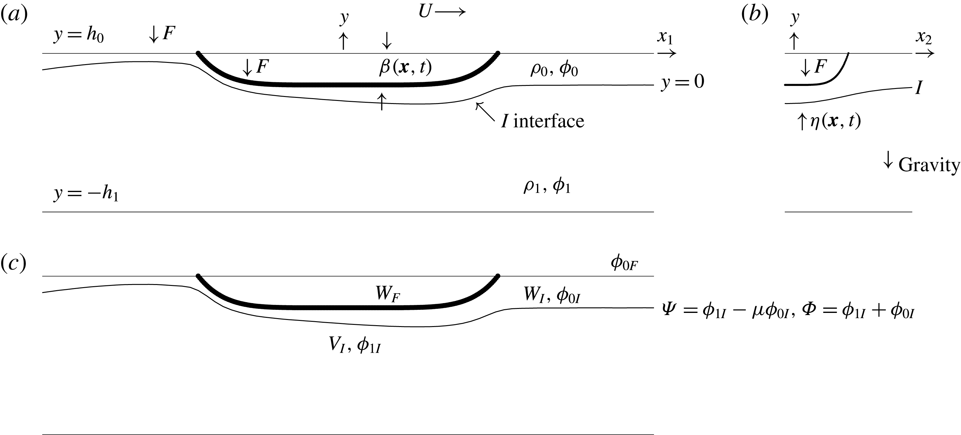
, determines the hull shape and is specified in (3.1) below. A definition sketch is found in figure 1. Following Grue (Reference Grue2015b
) we denote by
 $F$
the upper boundary of the upper fluid 0. The kinematic boundary condition along the ship hull is given by
 $\unicode[STIX]{x2202}\unicode[STIX]{x1D6FD}/\unicode[STIX]{x2202}t+W_{F}=0$
, where the normal velocity
 $W_{F}=\boldsymbol{U}\boldsymbol{\cdot }\unicode[STIX]{x1D735}_{H}\unicode[STIX]{x1D6FD}$
is connected to the fluid motion by
 $$\begin{eqnarray}\displaystyle W_{F}=\frac{\unicode[STIX]{x2202}\unicode[STIX]{x1D719}_{0}}{\unicode[STIX]{x2202}n}\sqrt{1+|\unicode[STIX]{x1D735}_{H}\unicode[STIX]{x1D6FD}|^{2}}=-\frac{\unicode[STIX]{x2202}\unicode[STIX]{x1D719}_{0}}{\unicode[STIX]{x2202}y}+\unicode[STIX]{x1D735}_{H}\unicode[STIX]{x1D6FD}\boldsymbol{\cdot }\unicode[STIX]{x1D735}_{H}\unicode[STIX]{x1D719}_{0}\quad \text{at }y=h_{0}+\unicode[STIX]{x1D6FD}. & & \displaystyle\end{eqnarray}$$
Here,
 $\unicode[STIX]{x1D735}_{H}=(\unicode[STIX]{x2202}/\unicode[STIX]{x2202}x_{1},\unicode[STIX]{x2202}/\unicode[STIX]{x2202}x_{2})$
denotes the horizontal gradient. The normal vector points into fluid 0. The potential evaluated at the position of the ship hull is introduced by
 $\unicode[STIX]{x1D719}_{0F}(\boldsymbol{x},t)=\unicode[STIX]{x1D719}(\boldsymbol{x},y=h_{0}+\unicode[STIX]{x1D6FD}(\boldsymbol{x},t),t)$
. The Froude number of the surface waves based on the ship length is
 $U/\sqrt{gl_{0}}\ll 1$
(where
 $g$
is the acceleration of gravity) and means that the rigid-lid condition can be applied along
 $F$
, outside the ship model, where
 $y=h_{0}$
. The relative roles of the internal and surface waves can be evaluated by calculating the wave resistance. This is further discussed in § 3.1, finding that the surface wave amplitude due to the observed ship is less than 4 % of the internal wave amplitude, where also the dead water resistance exceeds that of the surface waves.
Sketch of the two-fluid model. (a) Centre plane section, side view. (b) Mid ship section, frontal view. (c) Flow variables.

The Froude number in relation to the internal wave mode is defined by
 $Fr=U/c_{0}$
, where
 $c_{0}$
denotes the interfacial (internal) long-wave speed of the two-fluid system, given by
 $c_{0}^{2}=g^{\prime }h_{0}/(\unicode[STIX]{x1D70C}_{0}/\unicode[STIX]{x1D70C}_{1}+h_{0}/h_{1})$
, where
 $g^{\prime }=g(\unicode[STIX]{x1D70C}_{1}-\unicode[STIX]{x1D70C}_{0})/\unicode[STIX]{x1D70C}_{1}$
denotes reduced gravity. Let the interface be denoted by
 $I$
and its motion described by the elevation
 $y=\unicode[STIX]{x1D702}(x_{1},x_{2},t)$
, where
 $y=0$
determines the interface at rest. Values of the potentials along
 $I$
are introduced by
 $\unicode[STIX]{x1D719}_{0I}(\boldsymbol{x},t)=\unicode[STIX]{x1D719}_{0}(\boldsymbol{x},y=\unicode[STIX]{x1D702},t)$
and
 $\unicode[STIX]{x1D719}_{1I}(\boldsymbol{x},t)=\unicode[STIX]{x1D719}_{1}(\boldsymbol{x},y=\unicode[STIX]{x1D702},t)$
at
 $I$
. Scaled normal velocities along
 $I$
are introduced by
 $$\begin{eqnarray}\displaystyle W_{I}=\frac{\unicode[STIX]{x2202}\unicode[STIX]{x1D719}_{0}}{\unicode[STIX]{x2202}n}\sqrt{1+|\unicode[STIX]{x1D735}_{H}\unicode[STIX]{x1D702}|^{2}}\quad \text{and}\quad V_{I}=\frac{\unicode[STIX]{x2202}\unicode[STIX]{x1D719}_{1}}{\unicode[STIX]{x2202}n}\sqrt{1+|\unicode[STIX]{x1D735}_{H}\unicode[STIX]{x1D702}|^{2}}\quad \text{at }I & & \displaystyle\end{eqnarray}$$
for the upper and lower fluid respectively, where
 $n$
points into the upper fluid 0 (see figure 1).
Solution of the Laplacian potentials
 $\unicode[STIX]{x1D719}_{0}$
and
 $\unicode[STIX]{x1D719}_{1}$
is expressed by a set of integral equations, see Grue (Reference Grue2015a
,Reference Grue
b
). The velocities
 $W_{I}$
,
 $V_{I}$
along
 $I$
and potential
 $\unicode[STIX]{x1D719}_{0F}$
along
 $F$
are obtained using the method of successive approximations (e.g. Mikhlin Reference Mikhlin1957):
 $$\begin{eqnarray}\displaystyle \left.\begin{array}{@{}c@{}}W_{I}=W_{I}^{(1)}+W_{I}^{(2)}+W_{I}^{(3)}+\cdots \,,\quad V_{I}=V_{I}^{(1)}+V_{I}^{(2)}+V_{I}^{(3)}+\cdots \,,\\ \unicode[STIX]{x1D719}_{0F}=\unicode[STIX]{x1D719}_{0F}^{(1)}+\unicode[STIX]{x1D719}_{0F}^{(2)}+\unicode[STIX]{x1D719}_{0F}^{(3)}+\cdots \,.\end{array}\right\} & & \displaystyle\end{eqnarray}$$
The leading linear approximation of the set of equations is obtained by the triple
 $(W_{I}^{(1)},V_{I}^{(1)},\unicode[STIX]{x1D719}_{0F}^{(1)})$
. The quadratic approximation, obtained by
 $(W_{I}^{(1)}+W_{I}^{(2)},V_{I}^{(1)}+V_{I}^{(2)},\unicode[STIX]{x1D719}_{0F}^{(1)}+\unicode[STIX]{x1D719}_{0F}^{(2)})$
, includes the leading coupling between the variables
 $\unicode[STIX]{x1D719}_{0}$
and
 $\unicode[STIX]{x2202}\unicode[STIX]{x1D719}_{0}/\unicode[STIX]{x2202}n$
, and
 $\unicode[STIX]{x1D719}_{1}$
and
 $\unicode[STIX]{x2202}\unicode[STIX]{x1D719}_{1}/\unicode[STIX]{x2202}n$
, as well as the excursions
 $\unicode[STIX]{x1D702}$
along
 $I$
and
 $\unicode[STIX]{x1D6FD}$
along
 $F$
, where
 $\unicode[STIX]{x1D6FD}$
is prescribed. The cubic approximation, obtained by
 $(W_{I}^{(1)}+W_{I}^{(2)}+W_{I}^{(3)},V_{I}^{(1)}+V_{I}^{(2)}+V_{I}^{(3)},\unicode[STIX]{x1D719}_{0F}^{(1)}+\unicode[STIX]{x1D719}_{0F}^{(2)}+\unicode[STIX]{x1D719}_{0F}^{(3)})$
, includes cubic couplings between the potentials, normal velocities and excursions along
 $I$
and the body geometry. The quadratic and cubic contributions have been implemented and tested in the two-dimensional case, where reference solutions for solitary waves of very large amplitude exist. Further, interfacial wave generation by a moving geometry in two dimensions has been tested. We refer to Grue (Reference Grue2015a
, figures 2–5, table 1), where it is documented that the expansions of the variables given in (2.3) above converge very rapidly for interfacial elevations up to the thinner layer depth (
 $h_{0}$
). Thus, for
 $\unicode[STIX]{x1D702}/h_{0}\sim 1$
the examples provided in Grue (Reference Grue2015a
) document that
 $|W_{I}^{(3)}|/|W_{I}^{(1)}+W_{I}^{(2)}+W_{I}^{(3)}|\simeq |W_{I}^{(3)}|/|W_{I}|\ll 1$
,
 $|V_{I}^{(3)}|/|V_{I}^{(1)}+V_{I}^{(2)}+V_{I}^{(3)}|\simeq |V_{I}^{(3)}|/|V_{I}|\ll 1$
. This means that
 $W_{I}^{(1)}+W_{I}^{(2)}$
and
 $V_{I}^{(1)}+V_{I}^{(2)}$
represent the full nonlinearity in the calculations for elevations up to
 $\unicode[STIX]{x1D702}/h_{0}\sim 1$
. This result contributes considerably to the computational speed and requirements of RAM. The evaluations of
 $W_{I}^{(1)}+W_{I}^{(2)}$
,
 $V_{I}^{(1)}+V_{I}^{(2)}$
imply an order of magnitude fewer products compared with
 $W_{I}^{(1)}+W_{I}^{(2)}+W_{I}^{(3)}$
,
 $V_{I}^{(1)}+V_{I}^{(2)}+V_{I}^{(3)}$
. As a result, computations can be performed for relatively large horizontal domains, where the opposite is true for evaluations including the cubic terms, where the correction terms provide contributions that are approximately zero.
Explicit expressions of the linear and quadratic contributions are obtained by use of the Fourier transform:
 $$\begin{eqnarray}\displaystyle & \displaystyle {\mathcal{F}}(W_{I}^{(1)})=-kT_{0}{\mathcal{F}}(\unicode[STIX]{x1D719}_{0I})-\frac{{\mathcal{F}}(W_{F})}{C_{0}}, & \displaystyle\end{eqnarray}$$
 $$\begin{eqnarray}\displaystyle & \displaystyle {\mathcal{F}}(W_{I}^{(2)})=kT_{0}{\mathcal{F}}(\unicode[STIX]{x1D702}W_{I}^{(1)})-\text{i}\boldsymbol{k}\boldsymbol{\cdot }{\mathcal{F}}(\unicode[STIX]{x1D702}\unicode[STIX]{x1D735}_{H}\unicode[STIX]{x1D719}_{0I})+\frac{\text{i}\boldsymbol{k}\boldsymbol{\cdot }{\mathcal{F}}(\unicode[STIX]{x1D6FD}\unicode[STIX]{x1D735}_{H}\unicode[STIX]{x1D719}_{0F})}{C_{0}}, & \displaystyle\end{eqnarray}$$
 $$\begin{eqnarray}\displaystyle & \displaystyle {\mathcal{F}}(V_{I}^{(1)})=kT_{1}{\mathcal{F}}(\unicode[STIX]{x1D719}_{1I}), & \displaystyle\end{eqnarray}$$
 $$\begin{eqnarray}\displaystyle & \displaystyle {\mathcal{F}}(V_{I}^{(2)})=-kT_{1}(\unicode[STIX]{x1D702}V_{I}^{(1)})-\text{i}\boldsymbol{k}\boldsymbol{\cdot }{\mathcal{F}}(\unicode[STIX]{x1D702}\unicode[STIX]{x1D735}_{H}\unicode[STIX]{x1D719}_{1I}), & \displaystyle\end{eqnarray}$$
 $$\begin{eqnarray}\displaystyle & \displaystyle {\mathcal{F}}(\unicode[STIX]{x1D719}_{0F}^{(1)})=\frac{{\mathcal{F}}(\unicode[STIX]{x1D719}_{0I})}{C_{0}}-\frac{T_{0}\,{\mathcal{F}}(W_{F})}{k}, & \displaystyle\end{eqnarray}$$
 $$\begin{eqnarray}\displaystyle & \displaystyle {\mathcal{F}}(\unicode[STIX]{x1D719}_{0F}^{(2)})=-\frac{{\mathcal{F}}(\unicode[STIX]{x1D702}W_{I}^{(1)})}{C_{0}}+\frac{T_{0}\,\text{i}\boldsymbol{k}}{k}\boldsymbol{\cdot }{\mathcal{F}}(\unicode[STIX]{x1D6FD}\unicode[STIX]{x1D735}_{H}\unicode[STIX]{x1D719}_{0F})-{\mathcal{F}}(\unicode[STIX]{x1D6FD}W_{F}). & \displaystyle\end{eqnarray}$$
Expressions for
 $W_{I}^{(3)}$
and
 $V_{I}^{(3)}$
are given in appendix D. Here,
 ${\mathcal{F}}$
denotes Fourier transform,
 ${\mathcal{F}}^{-1}$
inverse transform,
 $\boldsymbol{k}=(k_{1},k_{2})$
wavenumber vector in Fourier space and
 $k=|\boldsymbol{k}|$
. Further,
 $T_{0}=\tanh (kh_{0})$
,
 $T_{1}=\tanh (kh_{1})$
and
 $C_{0}=\cosh (kh_{0})$
. In (2.5) and (2.9),
 $\unicode[STIX]{x1D719}_{0F}=\unicode[STIX]{x1D719}_{0F}^{(1)}+\unicode[STIX]{x1D719}_{0F}^{(2)}$
. In the strongly nonlinear calculations presented below, the quadratic approximation is used. Linear calculations are obtained by using the triple
 $(W_{I}^{(1)},V_{I}^{(1)},\unicode[STIX]{x1D719}_{0F}^{(1)})$
.
The interfacial motion is expressed by the difference and sum potentials along the interface:
 $$\begin{eqnarray}\displaystyle \unicode[STIX]{x1D6F9}(\boldsymbol{x},t)=\unicode[STIX]{x1D719}_{1I}(\boldsymbol{x},t)-\unicode[STIX]{x1D707}\unicode[STIX]{x1D719}_{0I}(\boldsymbol{x},t)\quad \text{and}\quad \unicode[STIX]{x1D6F7}(\boldsymbol{x},t)=\unicode[STIX]{x1D719}_{1I}(\boldsymbol{x},t)+\unicode[STIX]{x1D719}_{0I}(\boldsymbol{x},t)\quad \text{at }I,\qquad \quad & & \displaystyle\end{eqnarray}$$
where
 $\unicode[STIX]{x1D707}=\unicode[STIX]{x1D70C}_{0}/\unicode[STIX]{x1D70C}_{1}$
denotes the density ratio. It should be noted that the jump function in (2.10a
) accounts for interactions between the density jump and ambient pressure fields. The interfacial elevation and jump in potential along
 $I$
are integrated forward in time using the kinematic and dynamic boundary conditions at the interface, giving
 $$\begin{eqnarray}\displaystyle \unicode[STIX]{x1D702}_{t}=V_{I}=W_{I},\quad \unicode[STIX]{x1D6F9}_{t}+g^{\prime }\unicode[STIX]{x1D702}={\mathcal{N}}{\mathcal{L}}_{2},\quad \text{ both at }I, & & \displaystyle\end{eqnarray}$$
where
 $g^{\prime }$
is defined below (2.1). The right-hand side of (2.11b
) is
 $$\begin{eqnarray}\displaystyle \hspace{-12.0pt}\mathscr{N}\mathscr{L}_{2} & = & \displaystyle -\frac{|\unicode[STIX]{x1D735}_{H}\unicode[STIX]{x1D719}_{1I}|^{2}-\unicode[STIX]{x1D707}|\unicode[STIX]{x1D735}_{H}\unicode[STIX]{x1D719}_{0I}|^{2}-(1-\unicode[STIX]{x1D707})W_{I}^{2}}{2+2|\unicode[STIX]{x1D735}_{H}\unicode[STIX]{x1D702}|^{2}}\nonumber\\ \displaystyle & & \displaystyle -\,\frac{-2W_{I}\unicode[STIX]{x1D735}_{H}\unicode[STIX]{x1D702}\boldsymbol{\cdot }\unicode[STIX]{x1D735}_{H}(\unicode[STIX]{x1D719}_{1I}-\unicode[STIX]{x1D707}\unicode[STIX]{x1D719}_{0I})+|\unicode[STIX]{x1D735}_{H}\unicode[STIX]{x1D702}\times \unicode[STIX]{x1D735}_{H}\unicode[STIX]{x1D719}_{1I}|^{2}-\unicode[STIX]{x1D707}|\unicode[STIX]{x1D735}_{H}\unicode[STIX]{x1D702}\times \unicode[STIX]{x1D735}_{H}\unicode[STIX]{x1D719}_{0I}|^{2}}{2+2|\unicode[STIX]{x1D735}_{H}\unicode[STIX]{x1D702}|^{2}},\nonumber\\ \displaystyle & & \displaystyle\end{eqnarray}$$
and is evaluated in the nonlinear calculations. In the linear calculations,
 $\mathscr{N}\mathscr{L}_{2}$
is put to zero. Successive approximations of the potential sum
 $\unicode[STIX]{x1D719}_{0I}+\unicode[STIX]{x1D719}_{1I}=\unicode[STIX]{x1D6F7}=\unicode[STIX]{x1D6F7}^{(1)}+\unicode[STIX]{x1D6F7}^{(2)}+\cdots$
are obtained by applying continuity of the normal velocity along the interface, using the expansions for
 $V_{I}$
and
 $W_{I}$
. The potentials
 $\unicode[STIX]{x1D719}_{0I}$
and
 $\unicode[STIX]{x1D719}_{1I}$
are then obtained. An RK4 scheme is used for time integration of the Fourier transformed versions of (2.11). The numerical method and implementation are described in Grue (Reference Grue2015a
,Reference Grue
b
).
3 Wave wake and resistance
The ship geometry is modelled by
 $$\begin{eqnarray}\displaystyle \unicode[STIX]{x1D6FD}(x_{1},x_{2},t)=-d_{0}\left(1-\left(\frac{x_{1}-x_{1,0}(t)}{l_{0}/2}\right)^{6}-\left(\frac{x_{2}}{w_{0}/2}\right)^{6}\right), & & \displaystyle\end{eqnarray}$$
where
 $l_{0}$
denotes the ship length,
 $w_{0}$
the width,
 $d_{0}$
the draught and
 $x_{1,0}(t)$
the prescribed position of the ship where
 $U={\dot{x}}_{1,0}$
(note that
 $\unicode[STIX]{x1D6FD}\leqslant 0$
). We perform computations relevant to a set of field observations of the wave wake generated by a cargo ship moving along a Canadian fjord; see the description in § 4.1 below. In the observations, an upper mixed layer of depth 5 m is separated from a deep lower salty layer by a 5 m thick pycnocline localized at an average depth of 7.5 m. Applying the two-fluid model, we shall use
 $h_{0}=7.5~\text{m}$
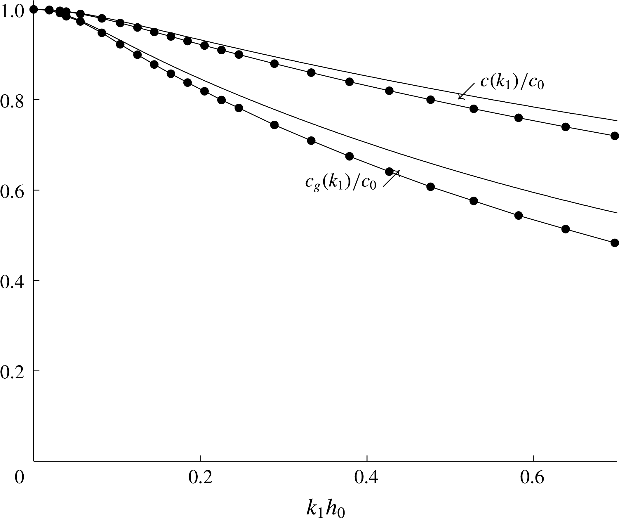
as the depth of the upper layer in the two-layer fluid. This is also the reference length for the computations. Wave propagation characteristics comparing two- and three-layer fluids, where in the latter the finite thickness of the pycnocline is accounted for, are described in appendix B, with results illustrated in figure 13, finding only minor differences between the wave phase speeds and group velocities of the two- and three-layer fluids for
 $k_{1}h_{0}<0.7$
(where
 $k_{1}$
is the wavenumber along the
 $x_{1}$
-direction). The asymptotic wave wake patterns of the two- and three-layer fluids are compared in figure 14(b) for the background density conditions in the Canadian fjord. We note that a two-layer representation of internal waves moving along a pycnocline of small or moderately finite thickness is further justified by the wave tank experiments by Grue et al. (Reference Grue, Jensen, Rusås and Sveen1999) and the three-layer calculations by Fructus & Grue (Reference Fructus and Grue2004).
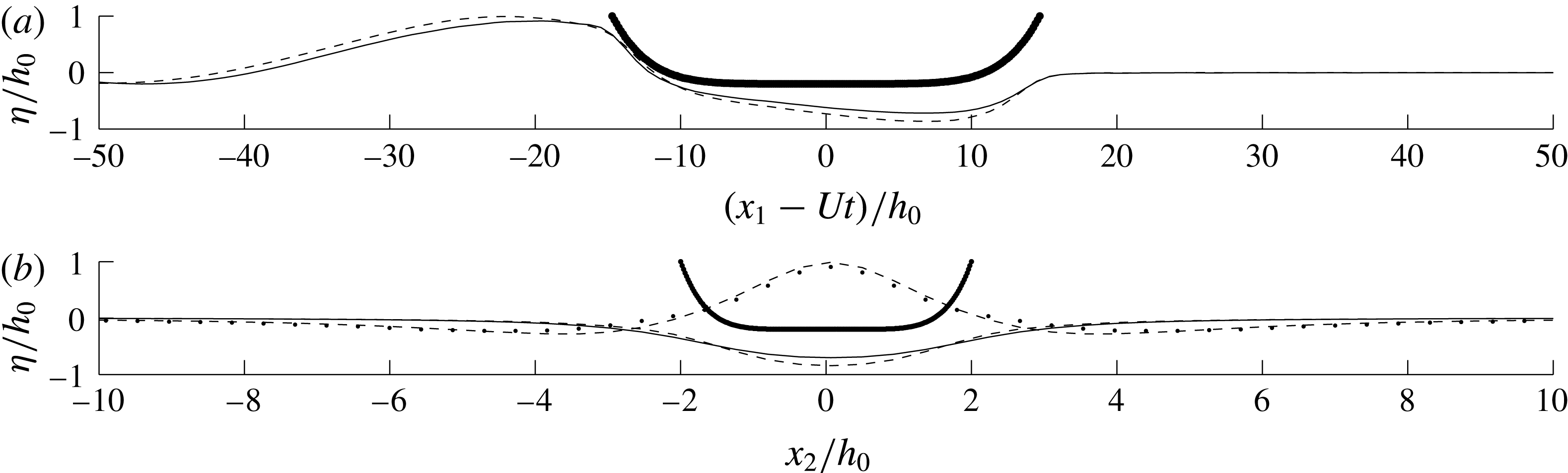
(a) The elevations
 $\unicode[STIX]{x1D702}_{NL}$
(—-) and
 $\unicode[STIX]{x1D702}_{LIN}$
(- - -) at the centre plane section (
 $x_{2}=0$
).(b) The elevations
 $\unicode[STIX]{x1D702}_{NL}$
(—-) and
 $\unicode[STIX]{x1D702}_{LIN}$
(- - -) at the lateral section at
 $(x_{1}-Ut)/h_{0}=9.6$
;
 $\unicode[STIX]{x1D702}_{NL}$
(
 $\cdots \,$
) and
 $\unicode[STIX]{x1D702}_{LIN}$
(- - -) at
 $(x_{1}-Ut)/h_{0}=-20.3$
. Section of the ship geometry at
 $(x_{1}-Ut)/h_{0}=0$
;
 $Fr=6.6$
,
 $(l_{0},w_{0},d_{0})=(29.4h_{0},4h_{0},1.2h_{0})$
; same computations as in figure 3(a,b).

The observed ship has the following dimensions: length 221 m, width 23 m and draught 9 m. The corresponding non-dimensional length and width are
 $l/h_{0}=29.4$
and
 $w/h_{0}=3$
respectively. The draught of 9 m corresponds to a non-dimensional draught of
 $d_{0}/h_{0}=1.2$
. In the computations, the degree of nonlinearity is investigated by varying this parameter in the range
 $d_{0}/h_{0}\sim 0.1{-}1.2$
. A ship draught of
 $d_{0}/h_{0}=0.1$
gives a wave wake well within the linear regime, while
 $d_{0}/h_{0}=1.2$
gives a strongly nonlinear interaction between the body and the interface, corresponding to the ship in the observation. The volume of the numerical ship, with dimensions
 $(l_{0},w_{0},d_{0})=(29.4h_{0},4h_{0},1.2h_{0})$
, becomes
 $V_{0}=43\,000~\text{m}^{3}$
(with
 $h_{0}=7.5~\text{m}$
), corresponding to the volume of the ship in the observation. Non-vertical ship walls at the waterline are assumed with the present mathematical and numerical formulation. In order to keep the sectional area of the ship, and thereby the volume, the width of the ship at the waterline is somewhat greater than the vertically averaged width. In the supercritical flow conditions, the interface is pushed down below the ship. Calculations of the steady motion may thus be performed for ship draughts that slightly exceed the interfacial level at rest where the nonlinear and linear interfaces below the ship are shown in figure 2. This is not true in the initial ramp-up phase in the calculations with
 $d_{0}/h_{0}$
slightly exceeding 1. The interface rapidly converges to the supercritical position, however. Alternatively, the draught may be gradually increased up to its final value. This has not been necessary. In the present formulation the local draught of the ship geometry is assumed to be a single-valued function of the horizontal coordinate; however, the body coordinates may be generalized to be locally ‘overhanging’, following the generalizations presented in Clamond & Grue (Reference Clamond and Grue2001, appendix B.3) in two dimensions. Steady trim and pitch effects can be accounted for iteratively; however, they are quite small for a free-surface Froude number of
 $U/\sqrt{gl_{0}}=0.14$
, such as for the present observed ship.
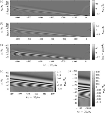
(a) Nonlinear elevation (
 $\unicode[STIX]{x1D702}_{NL}$
), (b) linear elevation (
 $\unicode[STIX]{x1D702}_{LIN}$
), (c) difference (
 $\unicode[STIX]{x1D702}_{NL}-\unicode[STIX]{x1D702}_{LIN}$
) of ship wake;
 $Fr=6.6$
,
 $tc_{0}/h_{0}=100$
. (d) Nonlinear elevation
 $\unicode[STIX]{x1D702}_{NL}$
far downstream, at
 $tc_{0}/h_{0}=135$
, and (e)
 $\unicode[STIX]{x1D702}_{NL}$
at
 $tc_{0}/h_{0}=195$
. Ship dimensions
 $(l_{0},w_{0},d_{0})=(29.4h_{0},4h_{0},1.2h_{0})$
. Centre position of ship model at
 $(x_{1}-Ut=0,x_{2}=0)$
.

Ship wakes are calculated for Froude numbers
 $Fr=U/c_{0}$
in the range 4–12, where
 $c_{0}$
is defined below (2.1). A numerical wave tank of (length, width) of
 $(L_{1}=700h_{0},L_{2}=260h_{0})$
is discretized with
 $(N_{1},N_{2})=(864,600)$
nodes along the respective directions. This means that
 $(\unicode[STIX]{x0394}x_{1}/h_{0},\unicode[STIX]{x0394}x_{2}/h_{0})=(0.81,0.43)$
. The nonlinear (
 $\unicode[STIX]{x1D702}_{NL}$
) and linear (
 $\unicode[STIX]{x1D702}_{LIN}$
) elevations in the wave wake are obtained for the ship model with draught
 $d_{0}/h_{0}=1.2$
moving along the
 $x_{1}$
-direction at
 $Fr=6.6$
. The running time is
 $t=100h_{0}/c_{0}$
; see figures 3(a,b). The depth ratio is
 $h_{1}/h_{0}=18$
, and
 $\unicode[STIX]{x0394}\unicode[STIX]{x1D70C}/\unicode[STIX]{x1D70C}\ll 1$
. The results illustrate that the difference
 $\unicode[STIX]{x1D702}_{NL}-\unicode[STIX]{x1D702}_{LIN}$
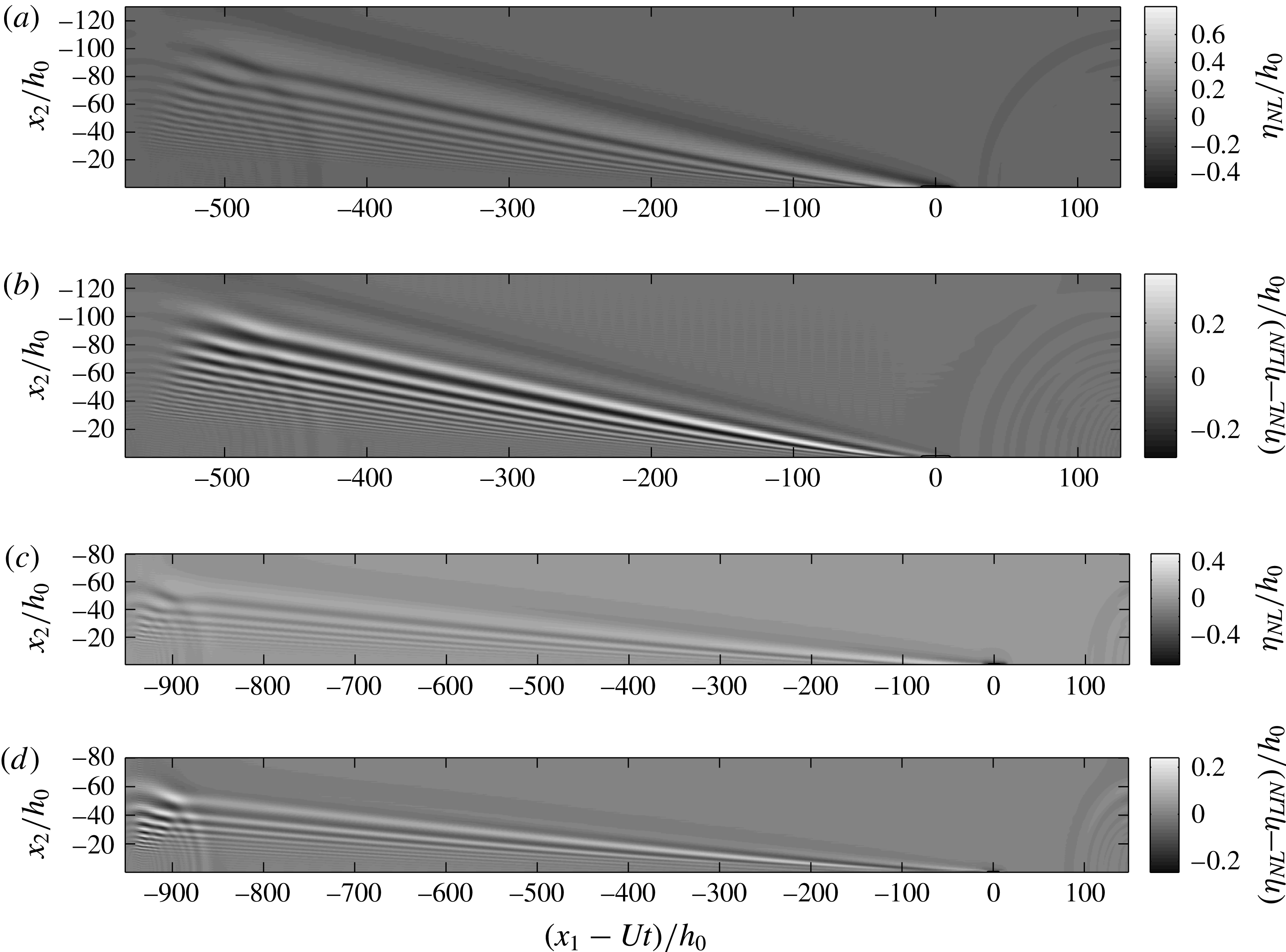
is comparable to the nonlinear elevation; see figures 3(c), 4(a)–(d), for
 $Fr\sim 4{-}12$
. Computations of the far downstream wave wake, for longer running times of
 $tc_{0}/h_{0}=135$
and
 $tc_{0}/h_{0}=195$
, are performed using wider and shorter wave tanks, and discretizations of respectively
 $(L_{1},L_{2})=(500h_{0},250h_{0})$
,
 $(N_{1},N_{2})=(720,720)$
(figure 3
d) and
 $(L_{1},L_{2})=(400h_{0},400h_{0})$
,
 $(N_{1},N_{2})=(500,1040)$
(figure 3
e). In these calculations the ship model is stopped after having traversed the distance
 $L_{1}$
.
(a) Nonlinear elevation (
 $\unicode[STIX]{x1D702}_{NL}$
) and (b) difference
 $\unicode[STIX]{x1D702}_{NL}-\unicode[STIX]{x1D702}_{LIN}$
of wave wake, for
 $Fr=4$
,
 $tc_{0}/h_{0}=140$
, for ship model of
 $(l_{0},w_{0},d_{0})=(29.4h_{0},4h_{0},0.8h_{0})$
. (c,d) The same for
 $Fr=12$
,
 $tc_{0}/h_{0}=80$
and ship model of
 $(l_{0},w_{0},d_{0})=(29.4h_{0},4h_{0},1.2h_{0})$
.

Wave wake elevations of numerical ships with draughts in the range
 $d_{0}/h_{0}\sim 0.1{-}1.2$
and Froude numbers of
 $Fr=4$
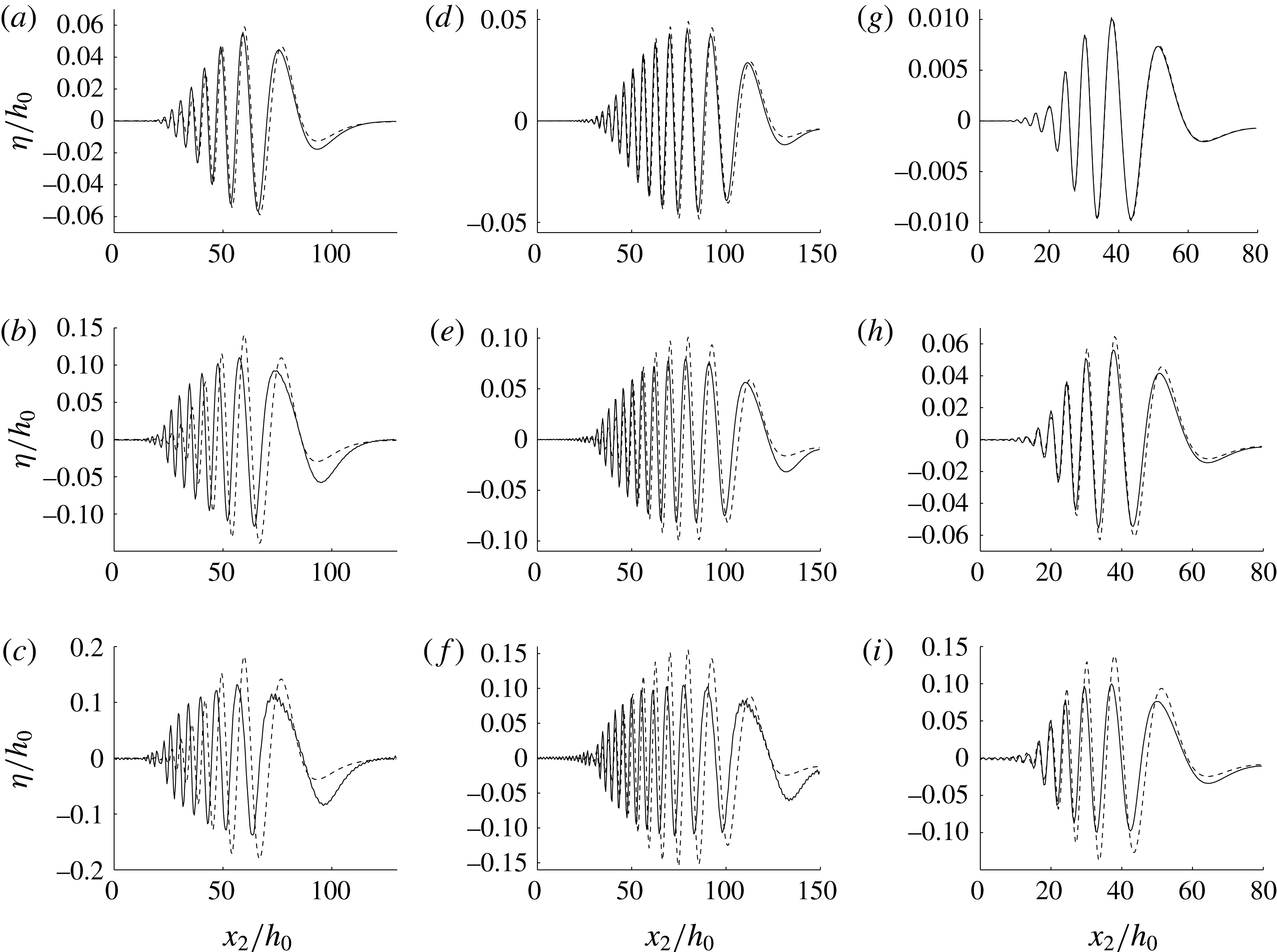
, 6.6 and 12 are obtained. The snapshots in figure 5 show the laterally moving wave train, where
 $\unicode[STIX]{x1D702}$
is a function of the lateral coordinate
 $x_{2}$
, at far downstream positions
 $x_{1}-Ut$
. An overprediction of the wave heights by up to 50 % is a main inferiority of the linear predictions. This occurs when the ship draught is comparable to the upper layer depth
 $(d_{0}/h_{0}\sim 1)$
. In figure 5(f), for
 $Fr=6.6$
and draught
 $d_{0}/h_{0}=1.2$
, the wave height is up to
 $0.2h_{0}$
in the nonlinear prediction and
 $0.3h_{0}$
in the linear prediction. The overprediction by the linear method is 39 % in figure 5(i), for
 $Fr=12$
,
 $d_{0}/h_{0}=1.2$
, and 34 % in figure 5(c), for
 $Fr=4$
,
 $d_{0}/h_{0}=0.9$
.
Nonlinear (solid line) and linear (dashed line) lateral elevation of wave wake at fixed downstream positions for increasing ship draught and Froude number: (a)–(c)
 $(x_{1}-Ut)/h_{0}=92.6$
,
 $Fr=4$
, ship draught
 $d_{0}/h_{0}=0.3,0.7,0.9$
; (d)–(f)
 $(x_{1}-Ut)/h_{0}=133.3$
,
 $Fr=6.6$
, ship draught
 $d_{0}/h_{0}=0.4,0.8,1.2$
; (g)–(i)
 $(x_{1}-Ut)/h_{0}=66.6$
,
 $Fr=12$
, ship draught
 $d_{0}/h_{0}=0.1,0.6,1.2$
. The ship model has length
 $l_{0}=29.4h_{0}$
and width
 $w_{0}=4h_{0}$
.

What is even more important is the representation of the leading part of the diverging wave train, where the nonlinear leading trough is pronounced, while its linear counterpart totally misrepresents the wave and also moves too slowly. The appreciable leading nonlinear trough including its forerunning slope is very important in the interpretation of what is identified as the leading diverging wave in the field observation described below. This is found to move at supercritical speed; see the discussion in § 5.2.
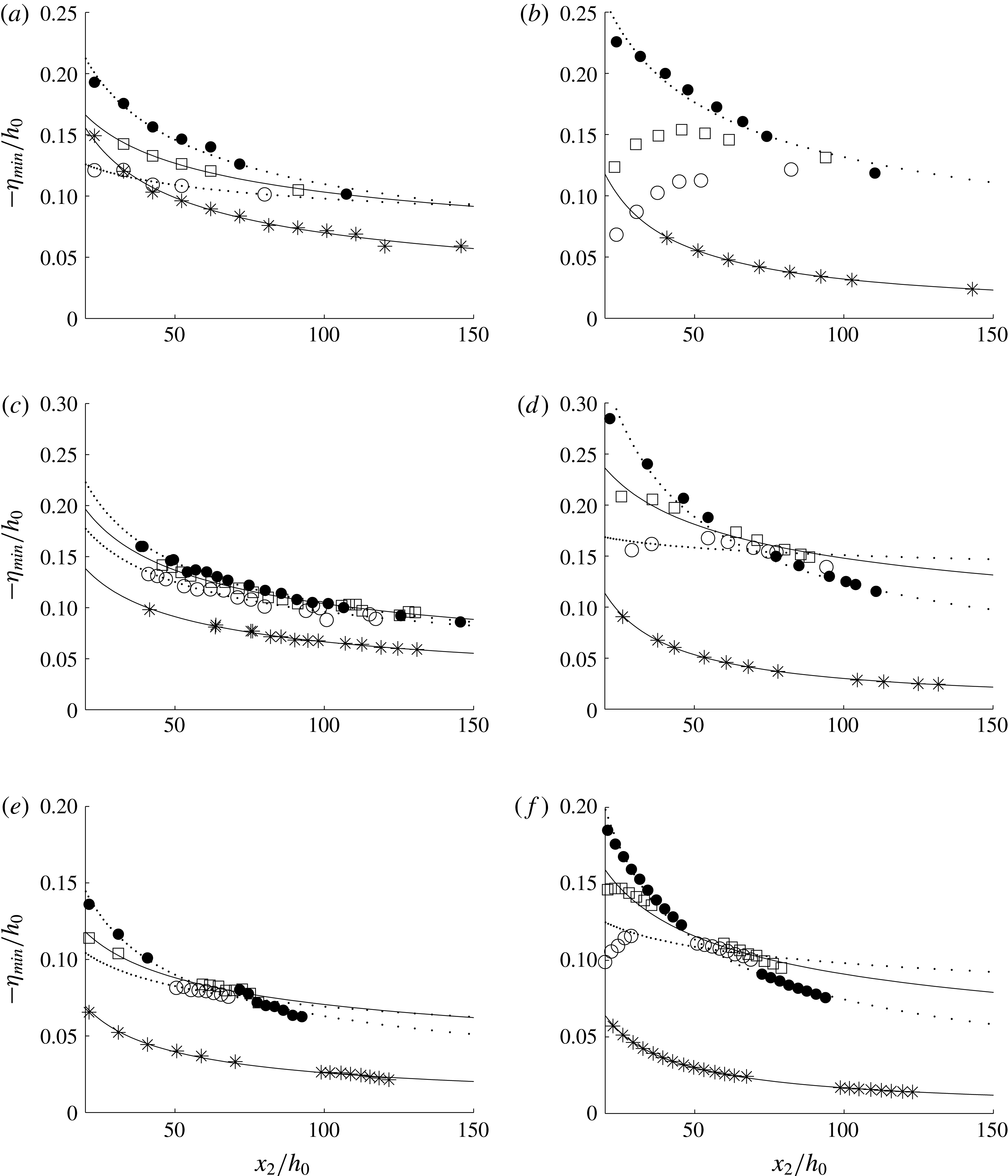
The negative excursions along the first four troughs are obtained for a ship draught of
 $d_{0}/h_{0}=0.8$
and
 $Fr=4$
, and
 $d_{0}/h_{0}=1.2$
and
 $Fr=6.6$
and 12. The depressions are obtained as functions of the lateral coordinate; see figure 6. Following studies on ship-generated surface wave wakes, the wave height of the diverging waves exhibits an algebraic decay in the lateral coordinate according to
 $x_{2}^{-\unicode[STIX]{x1D6FC}}$
, where the exponent
 $\unicode[STIX]{x1D6FC}$
is in the range between
 $0.2$
and
 $1.06$
; see Doctors & Zilman (Reference Doctors and Zilman2004). The trough amplitudes,
 $\unicode[STIX]{x1D702}_{min}$
, in the present numerical experiments are similarly compared with
 $$\begin{eqnarray}\displaystyle \unicode[STIX]{x1D702}_{min}/h_{0}=-B(x_{2}/h_{0})^{-\unicode[STIX]{x1D6FC}}, & & \displaystyle\end{eqnarray}$$
where
 $B$
and
 $\unicode[STIX]{x1D6FC}$
are fitted. The exponent
 $\unicode[STIX]{x1D6FC}$
is in the range 0.46–0.61 for the leading trough, and in the range 0.41–0.52 for the second trough, both resulting from the nonlinear calculations. The decay is weaker for the third and fourth troughs, with
 $\unicode[STIX]{x1D6FC}\sim 0.30{-}0.40$
and
 ${\sim}0.16{-}0.38$
respectively. Values of the coefficient
 $B$
are obtained as well. The results in table 1 may be used to obtain trough amplitudes at any lateral
 $x_{2}$
and downstream position
 $x_{1}$
. Linearly calculated depressions along the wave troughs are inferior, as seen in figure 6 and table 1.
Nonlinear (left plots) and linear (right plots) elevation,
 $\unicode[STIX]{x1D702}_{min}$
, along troughs 1 to 4 in ship wake, versus lateral coordinate,
 $x_{2}$
: (a,b)
 $Fr=4$
, ship dimensions
 $(l_{0},w_{0},d_{0})=(29.4h_{0},4h_{0},0.8h_{0})$
; (c,d)
 $Fr=6.6$
, ship dimensions
 $(l_{0},w_{0},d_{0})=(29.4h_{0},4h_{0},1.2h_{0})$
; (e,f)
 $Fr=12$
, ship dimensions
 $(l_{0},w_{0},d_{0})=(29.4h_{0},4h_{0},1.2h_{0})$
; trough 1 (*), trough 2 (●), trough 3 (▫), trough 4 (○). Solid and dotted lines: fits of
 $\unicode[STIX]{x1D702}_{min}/h_{0}=-B(x_{2}/h_{0})^{-\unicode[STIX]{x1D6FC}}$
.

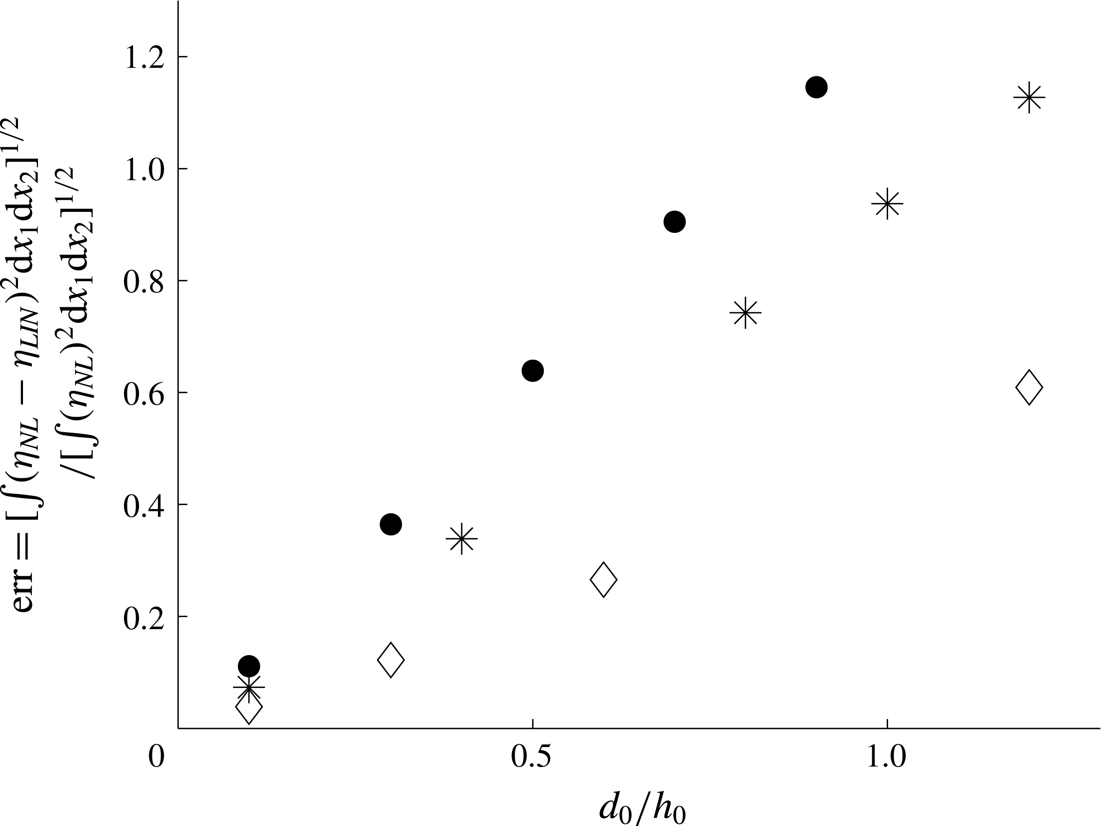
Root mean square (r.m.s.) values of the difference between the nonlinear and linear wave wake are compared with r.m.s. values of
 $\unicode[STIX]{x1D702}_{NL}$
; i.e. we divide
 $[\int _{\boldsymbol{x}}(\unicode[STIX]{x1D702}_{NL}-\unicode[STIX]{x1D702}_{LIN})^{2}\,\text{d}x_{1}\,\text{d}x_{2}]^{1/2}$
by
 $[\int _{\boldsymbol{x}}(\unicode[STIX]{x1D702}_{NL})^{2}\,\text{d}x_{1}\,\text{d}x_{2}]^{1/2}$
, where integration is carried out over the entire computational domain, after each run. The r.m.s. ratio, a function of the ship draught ratio (
 $d_{0}/h_{0}$
) and Froude number, is of order unity when
 $d_{0}/h_{0}\sim 1$
and
 $Fr=4$
and
 $Fr=6.6$
(figure 7). The relative difference reduces with increasing Froude number. Linear calculations are in general good only for very small draughts of the ship.
The r.m.s. value of
 $\unicode[STIX]{x1D702}_{NL}-\unicode[STIX]{x1D702}_{LIN}$
divided by the r.m.s. value of
 $\unicode[STIX]{x1D702}_{NL}$
versus the ship draught
 $d_{0}/h_{0}$
for
 $Fr=4$
(●),
 $Fr=6.6$
(*) and
 $Fr=12$
(♢).

Values
 $(\unicode[STIX]{x1D6FC},B)$
of fitted curves,
 $\unicode[STIX]{x1D702}_{min}/h_{0}=-B(x_{2}/h_{0})^{-\unicode[STIX]{x1D6FC}}$
, of troughs 1–4, obtained by nonlinear (NL) and linear (LIN) predictions. Ship model with
 $(l_{0},w_{0},d_{0})=(29.4h_{0},4h_{0},1.2h_{0})$
for
 $Fr=6.6$
and 12, and
 $(l_{0},w_{0},d_{0})=(29.4h_{0},4h_{0},0.8h_{0})$
for
 $Fr=4$
.

3.1 Internal wave resistance force
The pressure force on the ship along the motion direction due to the internal wave wake is given by
 $F_{1}=\int _{F}-pn_{1}\,\text{d}S$
, where integration is over the wetted body surface. The normal vector component along the
 $x_{1}$
-direction,
 $n_{1}$
, points into the fluid, and
 $n_{1}\,\text{d}S=\unicode[STIX]{x2202}\unicode[STIX]{x1D6FD}/\unicode[STIX]{x2202}x_{1}\,\text{d}\boldsymbol{x}$
. The pressure is given by the Bernoulli equation,
 $p=-\unicode[STIX]{x1D70C}_{0}(\unicode[STIX]{x2202}\unicode[STIX]{x1D719}_{0}/\unicode[STIX]{x2202}t+(1/2)|\unicode[STIX]{x1D735}\unicode[STIX]{x1D719}_{0}|^{2}+gy)+\text{const}$
. By use of Gauss’ theorem and the transport theorem the time-dependent force may be obtained by, see Grue (Reference Grue2015b
, equation (27)),
 $$\begin{eqnarray}\displaystyle F_{1}=-\unicode[STIX]{x1D70C}_{0}\frac{\text{d}}{\text{d}t}\int _{F}\frac{\unicode[STIX]{x2202}\unicode[STIX]{x1D719}_{0F}}{\unicode[STIX]{x2202}x_{1}}\,\unicode[STIX]{x1D6FD}\,\text{d}\boldsymbol{x}-\unicode[STIX]{x1D70C}_{0}U\int _{F}\frac{\unicode[STIX]{x2202}\unicode[STIX]{x1D719}_{0}}{\unicode[STIX]{x2202}x_{1}}\frac{\unicode[STIX]{x2202}\unicode[STIX]{x1D6FD}}{\unicode[STIX]{x2202}x_{1}}\,\text{d}\boldsymbol{x}+\frac{\unicode[STIX]{x1D70C}_{0}}{2}\int _{F}|\unicode[STIX]{x1D735}\unicode[STIX]{x1D719}_{0}|^{2}\frac{\unicode[STIX]{x2202}\unicode[STIX]{x1D6FD}}{\unicode[STIX]{x2202}x_{1}}\,\text{d}\boldsymbol{x}. & & \displaystyle\end{eqnarray}$$
This expression is used in the evaluations. The force attains, after a transient start-up, a steady value, and is obtained in non-dimensional terms by the internal wave resistance coefficient defined by
 $C_{R}=2F_{1}/\unicode[STIX]{x1D70C}_{0}SU^{2}$
, where
 $S$
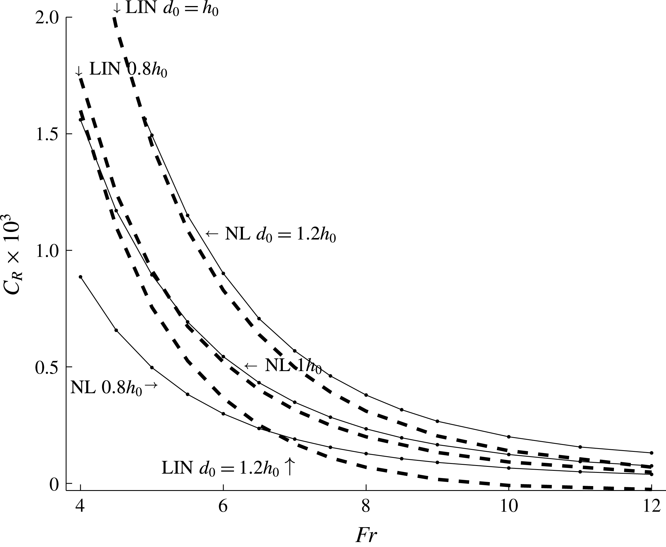
denotes the wetted surface area of the ship. The nonlinear calculations give a resistance coefficient of
 $C_{R}\sim 1.5\times 10^{-3}$
for the points
 $Fr=4,d_{0}=h_{0}$
and
 $Fr=5,d_{0}=1.2h_{0}$
. A resistance of
 $C_{R}\simeq 0.9\times 10^{-3}$
is obtained for the smaller draught of
 $d_{0}=0.8h_{0}$
and
 $Fr=4$
. The
 $C_{R}$
decays with increasing
 $Fr$
; see figure 8. We note that an internal wave resistance coefficient of
 $C_{R}\simeq 1.5\times 10^{-3}$
compares with the frictional drag coefficient, where the latter is
 $C_{F}\simeq 1.5\times 10^{-3}$
for a Reynolds number of
 $Re=Ul_{0}/\unicode[STIX]{x1D708}\simeq 1.5\times 10^{9}$
, where
 $U\simeq 6.6~\text{m}~\text{s}^{-1}$
and
 $l_{0}=221~\text{m}$
have been used; see Newman (Reference Newman1977, figure 2.12, p. 31). The wave wake resistance is thus comparable to the frictional resistance for
 $Fr\sim 4{-}6$
and ship draught
 $d_{0}\sim h_{0}$
. The frictional resistance dominates for ships with smaller draughts moving at higher
 $Fr$
.
Nonlinear (NL) (solid line) and linear (LIN) (dashed line) internal wave resistance coefficient
 $C_{R}=2F_{1}/\unicode[STIX]{x1D70C}SU^{2}$
versus
 $Fr$
, for draughts
 $d_{0}=0.8h_{0}$
,
 $1h_{0}$
and
 $1.2h_{0}$
, and
 $(l_{0},w_{0})=(29.4h_{0},4h_{0})$
.

A linear calculation using the potential
 $\unicode[STIX]{x1D719}_{0F}^{(1)}$
and its gradients gives a resistance force that exceeds the nonlinear calculation by almost 100 % for ship draughts of
 $d_{0}=h_{0}$
and
 $d_{0}=0.8h_{0}$
. For the larger draught of
 $d_{0}=1.2h_{0}$
, the resistance evaluation using
 $\unicode[STIX]{x1D719}_{0F}^{(1)}$
is approximately 50 % or less of the nonlinear force and even becomes negative for
 $Fr>9$
, however.
The relative roles of the internal and surface waves may eventually be judged by the wave resistance. Figure 8 gives a nonlinear internal wave resistance coefficient of
 $C_{R}\simeq 0.8\times 10^{-3}$
for
 $Fr=6.6$
and
 $d_{0}/h_{0}=1.2$
corresponding to the ship in the observation. According to Newman (Reference Newman1977, figure 6.18, p. 283), the resistance coefficient due to the surface ship waves is
 $0.5\times 10^{-3}$
for
 $U/\sqrt{gl_{0}}=0.14$
(where
 $l_{0}$
is the ship length). This implies that the corresponding energy flux of the internal waves provides an upper bound for the energy flux of the surface waves, giving the following relation:
 $g^{\prime }|A_{internal}|^{2}c_{g,internal}>g|A_{surface}|^{2}c_{g,surface}$
(where
 $A_{internal}$
is the characteristic internal wave amplitude,
 $A_{surface}$
is the characteristic surface wave amplitude,
 $c_{g,internal}$
is the group velocity of the internal waves and
 $c_{g,surface}$
is the group velocity of the surface waves). This gives
 $|A_{surface}/A_{internal}|<(\unicode[STIX]{x0394}\unicode[STIX]{x1D70C}/\unicode[STIX]{x1D70C})^{3/4}\simeq 0.04$
. This means that a characteristic surface wave amplitude is less than 4 % of a characteristic internal wave amplitude for the observed ship. The total resistance coefficient on the ship also increases from
 $1.5\times 10^{-3}+0.5\times 10^{-3}$
to
 $1.5\times 10^{-3}+0.5\times 10^{-3}+0.8\times 10^{-3}$
due to the internal wave drag, i.e. an increase of 40 %. This, in fact, affects the manoeuvrability of the ship.
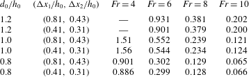
The dead water resistance coefficient
 $C_{R}$
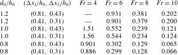
obtained by two different resolutions illustrates the convergence and accuracy of the method (table 2).
Internal wave resistance coefficient
 $C_{R}\times 10^{3}$
obtained by two different resolutions:
 $(\unicode[STIX]{x0394}x_{1}/h_{0},\unicode[STIX]{x0394}x_{2}/h_{0})=(0.81,0.43)$
and
 $(0.41,0.31)$
.
4 Field observations
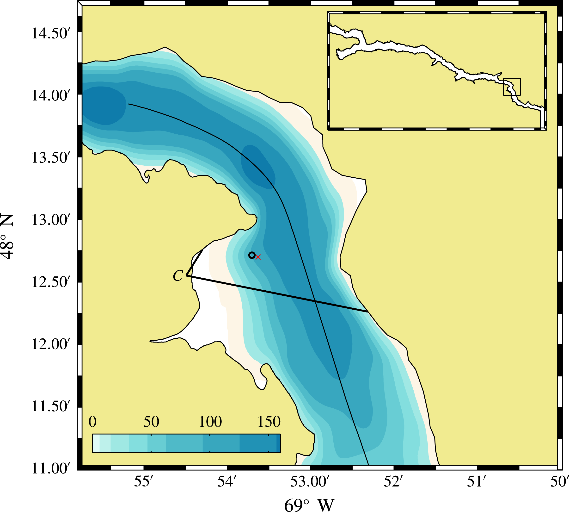
A two-week-long field experiment was carried out in June 2013 to observe the propagation of nonlinear internal waves and their reflection off a steep cliff in the Saguenay Fjord in Eastern Canada (figure 9). The experiment was motivated by the preliminary observations of internal wave reflection made by Bourgault, Janes & Galbraith (Reference Bourgault, Janes and Galbraith2011) in this environment. One piece of evidence of the generation and propagation of an internal wave train caused by the passage of a cargo ship was observed during the experiment, and the details of this event are presented here. More information about the general oceanography of this fjord can be found in Bourgault et al. (Reference Bourgault, Janes and Galbraith2011), Bourgault, Galbraith & Winkler (Reference Bourgault, Galbraith and Winkler2012) and Belzile, Galbraith & Bourgault (Reference Belzile, Galbraith and Bourgault2016) and references therein.
Map of the Saguenay Fjord and the bathymetry (in m). The symbol ‘C’ indicates the location of the time-lapse camera and its field of view (solid lines), and the circle indicates the position of the mooring. The curved solid line in the middle of the fjord is the Arctic ship track on 13 June obtained from the Automatic Identification System database. The red cross next to the mooring shows the position where a CTD cast was obtained at 20:30 UTC and used for comparison with the thermistor chain data (see figure 10 a,b for details).

In situ measurements were collected from a mooring equipped with a downward-looking 300 kHz Workhorse Sentinel acoustic Doppler current profiler (ADCP) manufactured by Teledyne RD Instruments. The ADCP was mounted on a gimbal installed inside a doughnut-like surface buoy in order to minimize pitch and roll caused by surface waves. Both pitch and roll stayed within
 $1^{\circ }$
for the duration of the internal ship wake event reported here. The ADCP pinging rate was 1.72 Hz and it recorded 10 s ensembles in 1 m vertical bin sizes. The compass calibration yielded an uncertainty of
 $\pm 7.8^{\circ }$
. The mooring was anchored in 80 m depth at
 $48^{\circ }~12.642^{\prime }~\text{N}$
,
 $69^{\circ }~53.719^{\prime }~\text{W}$
(figure 9). A GPS was installed on the buoy to measure its displacements.
The mooring was also equipped with eight temperature recorders (TR-1060 by RBR) and three temperature–depth recorders (TDR-2050) evenly distributed between 3.5 m and 38.5 m (3.5 m separation between each recorder). The three temperature–depth recorders were located at the top (3.5 m), middle (21.0 m) and end (38.5 m) of the temperature chain. The ADCP also recorded surface temperature at 0.5 m depth. Each RBR thermistor recorded at 1 Hz, while the ADCP recorded temperature in 10 s ensembles. Temperature–salinity profiles were also routinely carried out around the bay with a Seabird 19plus CTD profiler deployed from a small Zodiac.
Shore-based time-lapse photography also captured sea-surface patterns caused by internal waves, fronts and eddies in a way similar to that presented in Bourgault et al. (Reference Bourgault, Janes and Galbraith2011) and Richards et al. (Reference Richards, Bourgault, Galbraith, Hay and Kelley2013). We used a Canon EOS 40D with 10.1 megapixels located at
 $48^{\circ }~12.552^{\prime }~\text{N}$
,
 $69^{\circ }~54.492^{\prime }~\text{W}$
and altitude
 $H=50.5~\text{m}$
(figure 9). The camera recorded one image per minute. The images were calibrated to remove lens distortion and each image was stabilized against a reference image to remove small camera movements between successive images that may be caused by wind gusts. The calibrated and stabilized images were then georectified following Pawlowicz (Reference Pawlowicz2003), see also Bourgault (Reference Bourgault2008), using a series of 12 ground control points seen on site (boulders, capes, wharf, etc.). The r.m.s. difference between the ground control points and the georectified pixels is 10 m. The georectified image resolution is highly anisotropic with a much higher resolution in the horizontal field of view than in the vertical field of view due to the high obliquity of the images. The image resolution orthogonal to the line of sight and at the distance the ship passed, roughly 1 km away from the camera, is approximately 1 m. At the same distance, the resolution along the line of sight is approximately 20 m and steadily increases towards the camera.
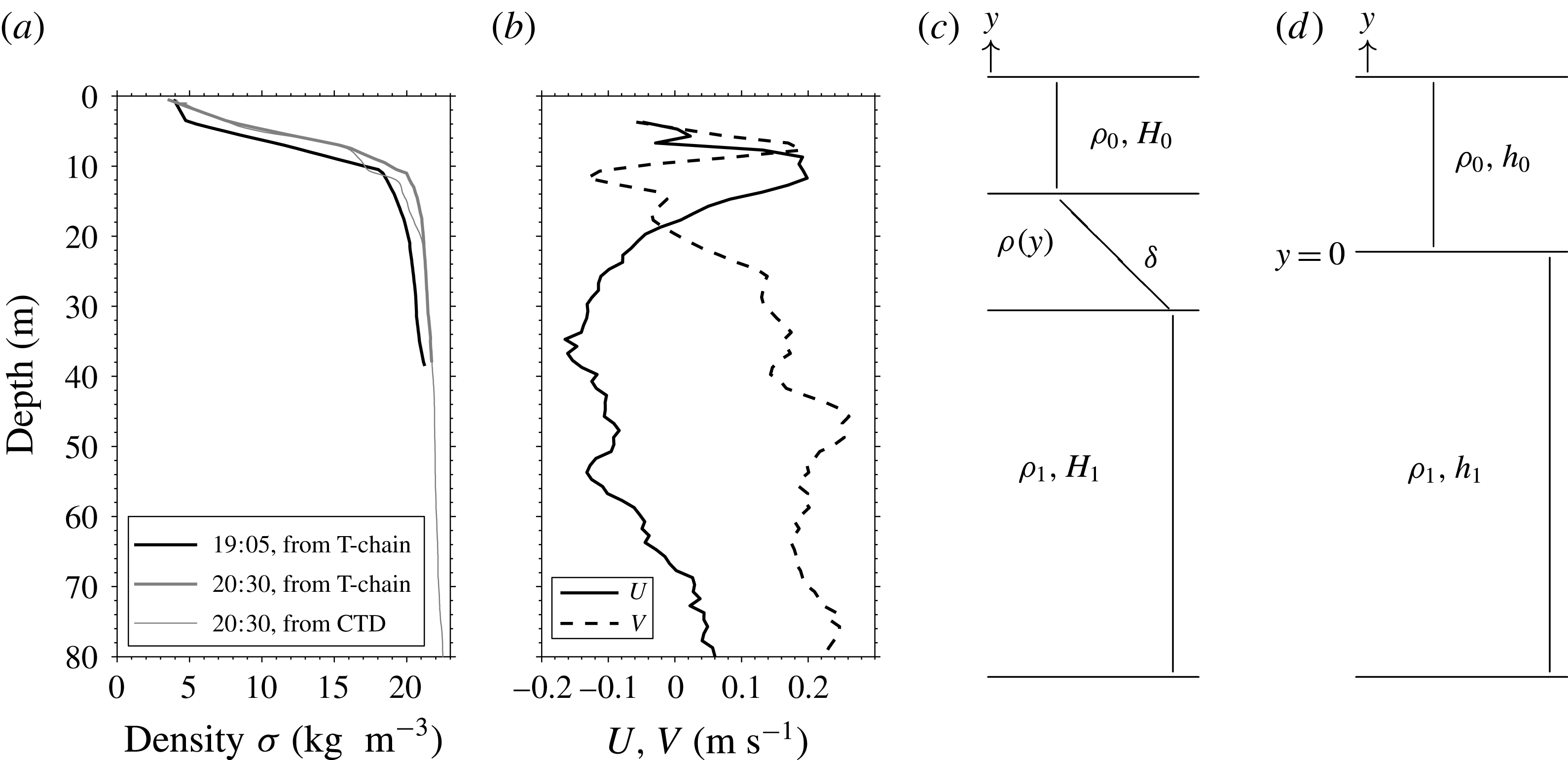
The background density structure is typical for this subarctic fjord, with a thin brackish surface layer overlying a thick salty bottom layer. These two layers are separated by a 5 m thick pycnocline located between 5 and 10 m and characterized by a density jump of
 $\unicode[STIX]{x0394}\unicode[STIX]{x1D70C}=15~\text{kg}~\text{m}^{-3}$
; see figure 10(a). The background conditions in the fjord, such as local velocity shear (figure 10
b), are further elaborated in appendix A.
Background conditions at the mooring site prior to the arrival of the internal wake. (a) The density profile at 19:05 UTC inferred from the thermistor chain and the T–S relationship (thick black). For comparison a CTD cast was obtained at 20:30 UTC next to the mooring (see figure 9 for the position of that cast) and is shown here (thin grey) along with the density inferred from the thermistors at the same moment (thick grey). (b) The eastward (solid) and northward (dashed) velocity profiles averaged over 15 min between 18:50 and 19:05. The uncertainty in this 15 min average is
 $\pm 0.01~\text{m}~\text{s}^{-1}$
. (c) Sketch of the theoretical three-layer fluid. (d) Two-layer fluid.

4.1 Internal wake
On 13 June, during calm conditions, a cargo ship was observed by the camera between 19:05 UTC and 19:08 UTC, moving south/south-east. According to the Canadian shipping traffic atlas (Simard et al.
Reference Simard, Roy, Giard and Yayla2014), this ship was the Arctic (Maritime Mobile Service Identity no. 316056000), with the following dimensions: length 221 m, width 23 m and draught 9 m. The Automatic Identification System (AIS) file provided 13 data points of position and speed between 19:05 and 19:07 UTC (see her track on figure 9). During this period, her mean speed over ground and standard deviation was
 $U_{ais}=6.57\pm 0.06~\text{m}~\text{s}^{-1}$
.
The information on ship length and speed provides an independent means to evaluate the accuracy of measurements taken from the georectified images. The ship length measured from the georectified images was very accurate, with
 $l_{img}=221\pm 1~\text{m}$
. The speed over ground determined from the four images where the ship was seen between 19:05 and 19:08 yielded
 $U_{img}=6.9\pm 0.3~\text{m}~\text{s}^{-1}$
. These measurements are consistent with the AIS data file.
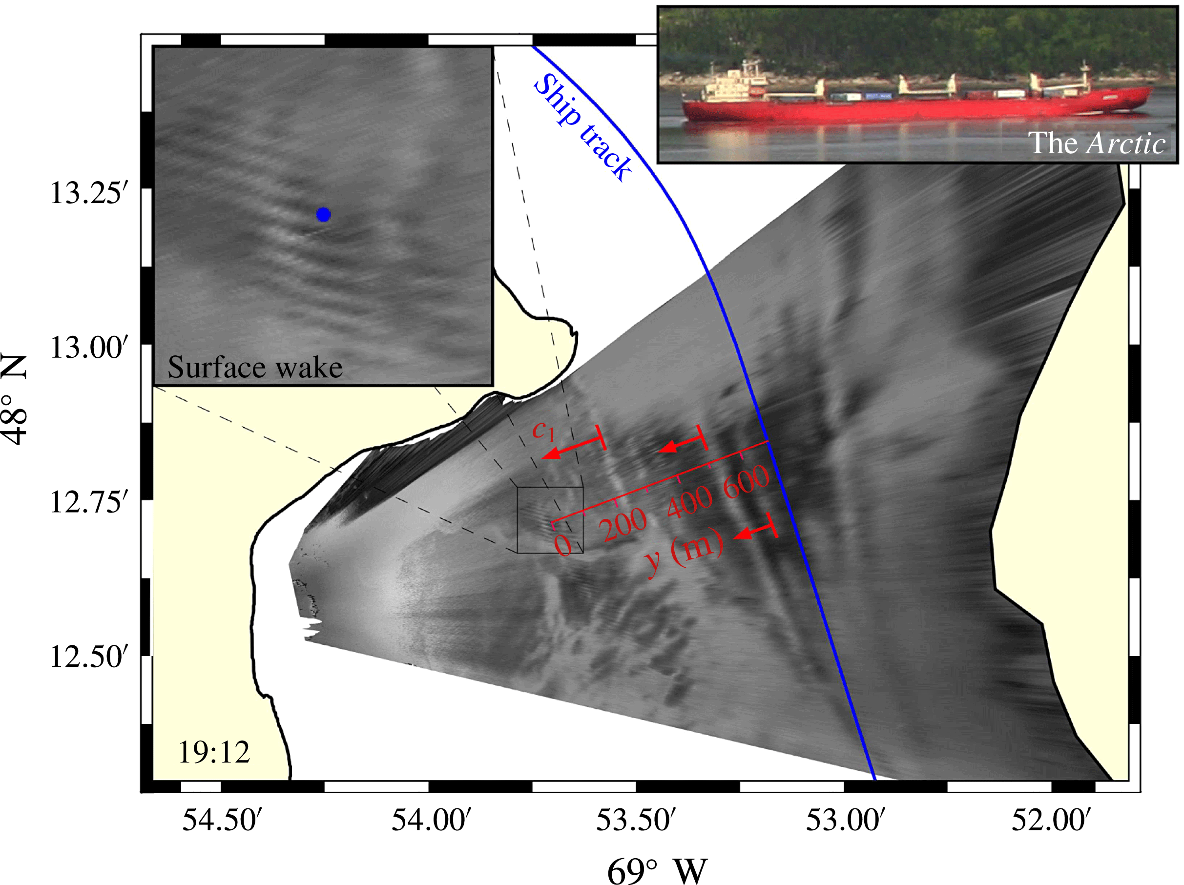
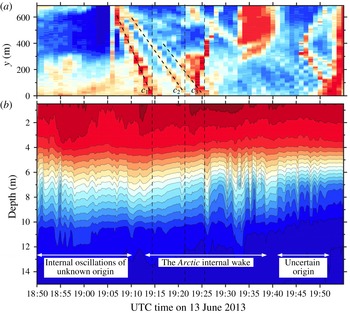
The georectified images showed that the passage of the ship created a V-like sea-surface wake that resembled the sea-surface signature of internal waves (figure 11). Measurements at the mooring confirmed that the surface propagating bands were coincident with 1–2 m isopycnal displacements riding on the pycnocline (figure 12). The ADCP did not clearly measure the waves due to too coarse temporal and vertical resolution.
Georectified image showing the sea-surface signature of the internal ship wake and the track caused by the Arctic. The leading beam (
 $c_{1}$
) and other beams are indicated by red lines and the mooring site is indicated by a blue circle.

Hovmöller diagrams (time–space) of (a) sea-surface patterns along the transect line running across the fjord orthogonal to the ship wake and going through the mooring location and (b) the density signal, inferred from the temperature measurements (see text) recorded at the mooring (
 $1~\text{kg}~\text{m}^{-3}$
per contour line). The phase speeds were determined by a best linear fit to the manually digitized beam seen in this image and identified as red lines labelled
 $c_{1}$
to
 $c_{3}$
. The values are
 $c_{1}=1.1\pm 0.04~\text{m}~\text{s}^{-1}$
,
 $c_{2}=0.69\pm 0.02~\text{m}~\text{s}^{-1}$
and
 $c_{3}=0.62\pm 0.02~\text{m}~\text{s}^{-1}$
.

A Hovmöller diagram of the pixel intensity re-interpolated along a transect line running across the fjord and taken orthogonal to the ship wake and going through the mooring location reveals the wave beams formed (figure 12). In this representation, the beam slope corresponds to the wave phase speed. A close inspection of the figure reveals a series of three prominent beams that have appeared after the passage of the ship. The first and fastest beam, identified as
 $c_{1}$
on the figure, has a phase speed of
 $c_{1}=1.1\pm 0.04~\text{m}~\text{s}^{-1}$
. The following two beams are coincident with vertical displacements of the isopycnals and have phase speeds of
 $c_{2}=0.69\pm 0.02~\text{m}~\text{s}^{-1}$
and
 $c_{3}=0.62\pm 0.02~\text{m}~\text{s}^{-1}$
respectively. Although only three wave beams are seen on the particular transect shown in figure 12, close inspection of the animated sequence of images reveals that up to 7–8 sea-surface bands are created by the passage of the ship (see the movie provided as supplementary material available at http://dx.doi.org/10.1017/jfm.2016.518).
5 Observation and theory compared
5.1 Wave heights of the wave wake
The linear long-wave speed of the two-layer fluid, see figure 10(d), is
 $c_{0}^{2lay}\simeq 1.0~\text{m}~\text{s}^{-1}$
, with
 $h_{0}=7.5~\text{m}$
,
 $h_{1}/h_{0}=18$
,
 $\unicode[STIX]{x0394}\unicode[STIX]{x1D70C}/\unicode[STIX]{x1D70C}\simeq 0.015$
, corresponding to the conditions in the field observation in the Saguenay Fjord, described in § 4 above. With a ship speed of approximately
 $6.6~\text{m}~\text{s}^{-1}$
this gives a Froude number of
 $Fr\simeq 6.6$
. We also evaluate the wave propagation speed of a three-layer fluid, accounting for a finite width of the pycnocline, for comparison with the two-layer fluid; see appendix B and figure 13. Differences in the wave speeds in the two- and three-layer fluids are small or moderate for the relatively long waves generated by the ship. The total water depth in the computations is 142.5 m (
 $h_{1}/h_{0}=18$
). The numerical vessel given in (3.1) has length, draught and displaced volume corresponding to the ship in the observation; see § 4.1. The non-dimensional draught is
 $d_{0}/h_{0}=1.2$
; see also further description of the geometry in the second paragraph in § 3.
Wave phase speed
 $c(k_{1})$
and group velocity
 $c_{g}(k_{1})$
, both normalized by the linear long-wave speeds of the respective density profiles. Two-layer configuration with
 $h_{1}/h_{0}=18$
(solid line) and three-layer configuration with
 $H_{1}/H_{0}=27.5$
,
 $\unicode[STIX]{x1D6FF}/H_{0}=1$
(solid line with dots).

The ship waves were observed at an off-track position of 687 m, corresponding to a lateral distance of
 $91.6h_{0}$
using
 $h_{0}=7.5~\text{m}$
as reference depth in the two-layer calculations. A series of three prominent wave beams riding on the pycnocline were measured after the passage of the ship, where isopycnal displacements were in the range 1–2 m; see § 4.1 and figure 12. It should be noted that altogether 7–8 sea-surface bands were observed. According to the nonlinear calculations in figure 5(f), see also figure 6(c), a wave train of eight waves has a wave height of
 $0.2h_{0}$
, corresponding to 1.5 m, with
 $h_{0}=7.5~\text{m}$
, fitting very well to the observation. A tail of smaller heights follows behind the main train. We note that, at the large off-track position of 687 m, the theoretical amplitude calculations assuming a thin pycnocline fit with the amplitude observations obtained for a pycnocline of 5 m thickness. This comparison indicates that a finite pycnocline thickness only implies a small variation in the algebraic decay compared with a very thin pycnocline. The comparison shows the usefulness of the power law in (3.2) for the internal wave wake regardless of pycnocline details. In contrast, the linear calculations predict a train of four waves of height
 $0.3h_{0}$
, corresponding to 2.3 m, which is taller than the observed value. We may also consult the results of the wave troughs in figure 6(c), where the nonlinear calculations show negative excursions of
 ${\sim}0.1h_{0}$
(0.75 m) along the second, third and fourth troughs, at a lateral distance of
 $91.6h_{0}$
. The similar linear calculations in figure 6(d) show, however, that the third and fourth wave troughs have depressions of
 ${\sim}0.15h_{0}$
(1.1 m) at
 $x_{2}=91.6h_{0}$
, i.e. 50 % higher than the nonlinear wave troughs. The excellent comparison between the nonlinear calculations and the observations of the far-field amplitude confirms the usefulness of the strongly nonlinear two-layer model. Conversely, the linear far-field amplitudes overpredict the observation. The number of waves is also lower than measured.
5.2 Wave speeds of the wave wake
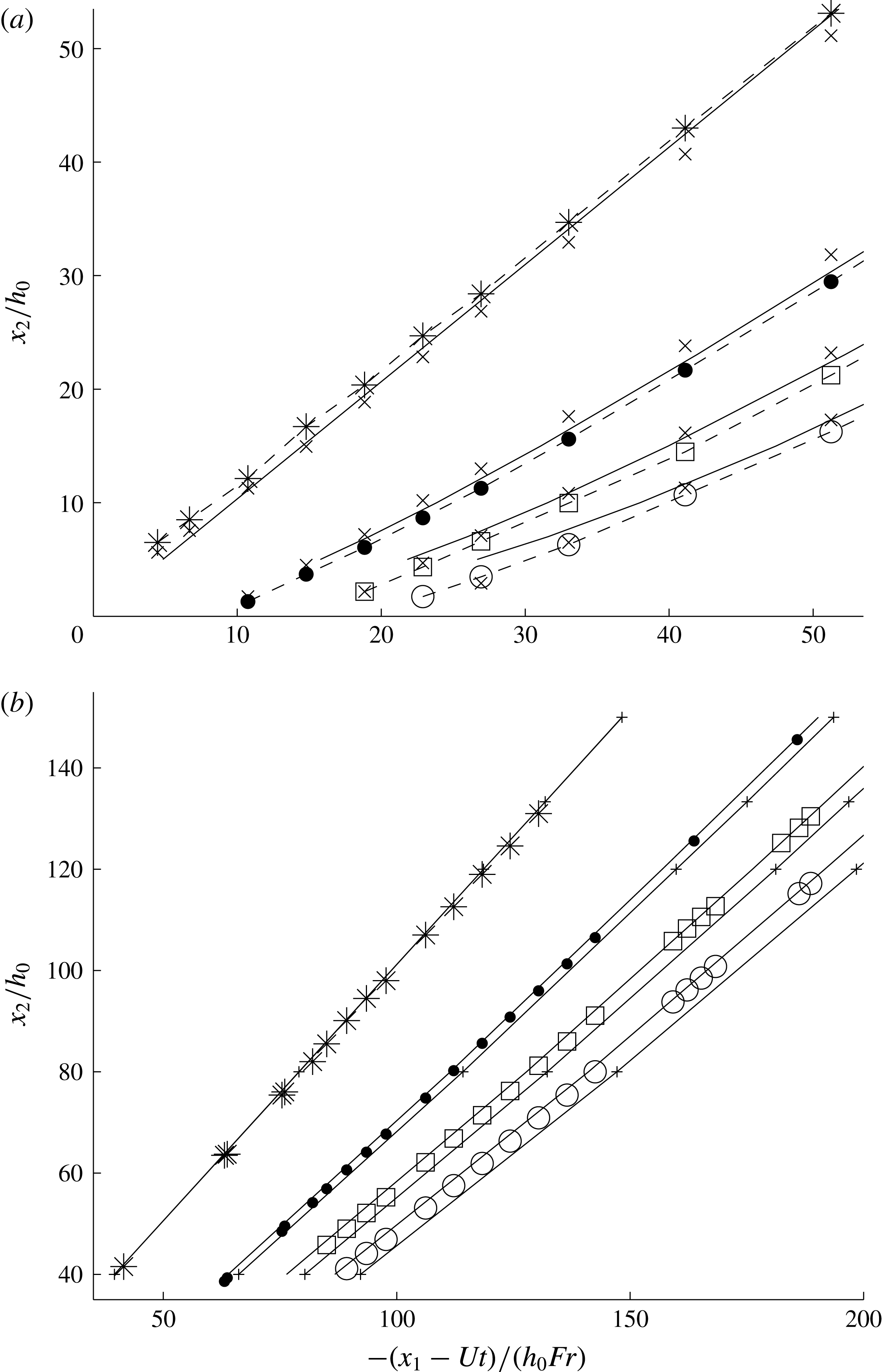
Nonlinear two-layer calculations of the wave trough pattern behind the complex ship geometry are presented together with the asymptotic patterns, where in the latter a disturbance located at the origin is assumed. The asymptotic patterns are evaluated for the two- and three-layer fluids using the equations given in appendix C. In the case of
 $Fr=4$
, the leading trough is systematically ahead of the asymptotic wave, while the subsequent troughs are behind the asymptotic waves, in the nonlinear calculations. In the linear calculations, the leading trough is behind the asymptotic pattern, while the second linear trough is ahead of the asymptotic one (figure 14
a). We note that a linear calculation of the wave pattern behind the ship geometry gives a leading wave trough slightly behind the leading nonlinear trough, while the subsequent linear wave troughs are slightly ahead of the nonlinear troughs (figure 5
c,f,i). These small differences are important. It should be noted that Tulin et al. (Reference Tulin, Yao and Wang2000) have presented a set of calculations accounting for the complex shape of their smaller model geometry. Their calculations fit exactly to the asymptotic pattern, even close to the geometry, where they calculate the positions of the crests and not the troughs. For
 $Fr=6.6$
, relevant to the conditions in the observations, the nonlinear evaluation of the trough pattern exhibits a close fit to the asymptotic pattern, however. Apart from the leading trough, the asymptotic troughs of the three-layer fluid are somewhat behind the troughs of the two-layer fluid (figure 14
b).
Trough positions of the wave wake: (a)
 $Fr=4$
,
 $d_{0}=0.8h_{0}$
,
 $h_{1}/h_{0}=18$
, nonlinear calculations, trough 1 (– – *), trough 2 (– – ●), trough 3 (– – ▫), trough 4 (– – ○); linear calculations,
 $\times$
; asymptotics (——); (b) nonlinear calculations (symbols), asymptotics for two-layer fluid (——), three-layer fluid with
 $H_{1}/H_{0}=27.5$
,
 $\unicode[STIX]{x1D6FF}/H_{0}=1$
(solid line with small
 $+$
) for
 $Fr=6.6$
,
 $d_{0}=1.2h_{0}$
.

For
 $Fr=6.6$
, the nonlinearly calculated wake angle fits very well to that of the asymptotic pattern, of
 $\sin ^{-1}(1/Fr)$
(e.g. Keller & Munk Reference Keller and Munk1970). In figure 14(b), the leading trough thus propagates laterally along the
 $x_{2}$
-axis with a speed of
 $c_{0}/\text{cos}(1/Fr)$
, in both the nonlinear and the asymptotic calculations, where
 $c_{0}$
denotes the long-wave speed of the two- or three-layer system. Figure 14(b) may be used to evaluate the lateral speeds of the wave beams in the observations, at the off-track recording position of 687 m, corresponding to
 $x_{2}=91.6h_{0}$
. The calculations are compared with the speeds of beams 1, 2 and 3, which in the field observation are respectively
 $c_{1}=1.1\pm 0.04~\text{m}~\text{s}^{-1}$
,
 $c_{2}=0.69\pm 0.02~\text{m}~\text{s}^{-1}$
and
 $c_{3}=0.62\pm 0.02~\text{m}~\text{s}^{-1}$
; see figure 12. Non-dimensional speeds are obtained by dividing by the linear long-wave speed of the stratified fjord assuming the three-layer model (appendix B), giving
 $c_{0}^{3lay}\simeq 0.97~\text{m}~\text{s}^{-1}$
; see table 3. The observed speeds of beams 2 and 3 fit very well to the calculated speeds of troughs 2 and 3.
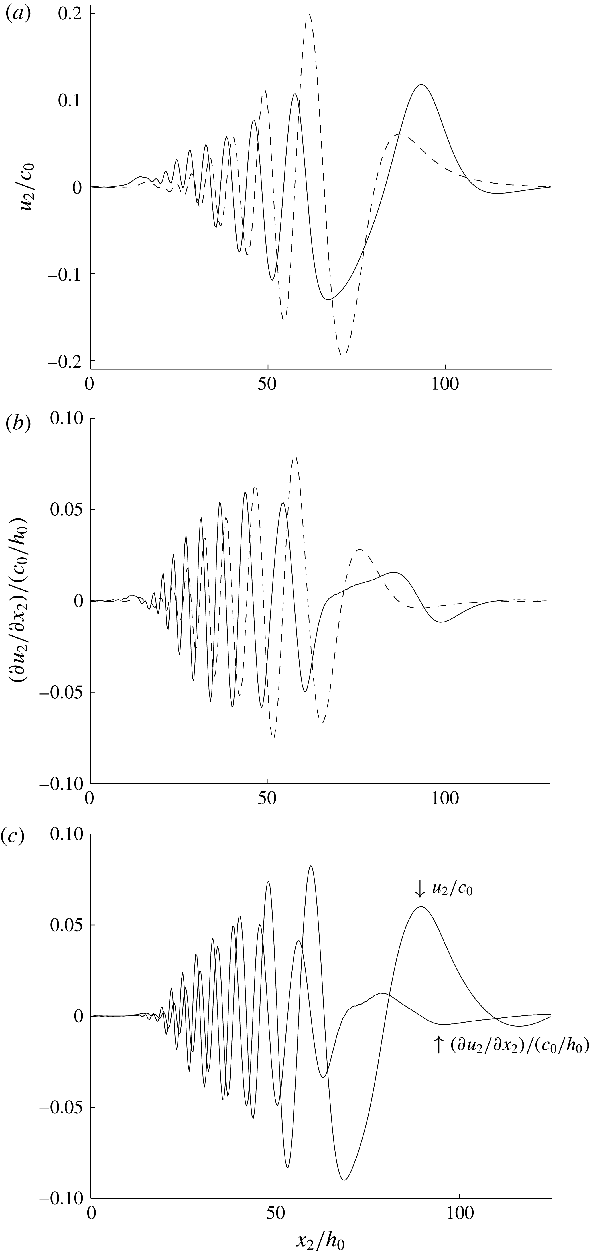
The speed of the observed leading beam is supercritical, however. This is moving faster than the leading trough. In the surface signatures of the internal waves it is not entirely clear what is observed. We have therefore evaluated the lateral surface velocity,
 $u_{2}$
, and its lateral derivative,
 $\unicode[STIX]{x2202}u_{2}/\unicode[STIX]{x2202}x_{2}$
, where the leading minimum of the latter is 7 % ahead of the leading maximum of
 $u_{2}$
, indicating a supercritical speed of the leading trough slope; see figure 15(c).
Nonlinear (——) and linear (– – –) (a) lateral surface velocity
 $u_{2}$
at
 $y=h_{0}$
, (b) strain rate
 $\unicode[STIX]{x2202}u_{2}/\unicode[STIX]{x2202}x_{2}$
at
 $y=h_{0}$
, both at
 $x_{1}-Ut=-500h_{0}$
, defined from the mean position of the ship;
 $Fr=5.7$
, ship model with length
 $38.8h_{0}$
, width
 $6.8h_{0}$
, draught
 $h_{0}$
; (c)
 $u_{2}$
and
 $\unicode[STIX]{x2202}u_{2}/\unicode[STIX]{x2202}x_{2}$
at
 $y=h_{0}$
at
 $x_{1}-Ut=582h_{0}$
; same calculation as in figure 3(d) for
 $Fr=6.6$
.

Observed travel speeds of beams 1–3 (column 2) and divided by
 $c_{0}^{3lay}$
(column 3). Trough speeds by three- and two-layer calculations (columns 4 and 5). Column 6: position of leading minimum of
 $\unicode[STIX]{x2202}u_{2}/\unicode[STIX]{x2202}x_{2}$
divided by position of leading maximum of
 $u_{2}$
at
 $x_{2}\simeq 91.6h_{0}$
. Nonlinear calculation.

5.3 Comparison with observations in Watson et al. (Reference Watson, Chapman and Apel1992)
Watson et al. (Reference Watson, Chapman and Apel1992) analysed a set of field experiments on ship-generated internal wave wakes performed in Loch Linnhe, Scotland. Results for one of the vessels in these experiments having the shallowest draught among the test ships, Sir Tristram, are compared with the present nonlinear model calculations. The ship had a waterline length of 116 m, width of 20 m and maximum draught of 3.9 m. The stratification in the measurements gave a linear long-wave speed of
 $c_{0}=0.35~\text{m}~\text{s}^{-1}$
of the waves of mode 1 and is here used to put the observational results for the velocities in the wake in non-dimensional form; see Watson et al. (Reference Watson, Chapman and Apel1992, figures 6 and 7). In the observations, a midlevel of the pycnocline corresponds to approximately 3 m. This is used as reference level for the two-layer model calculations, i.e. we use
 $h_{0}=3~\text{m}$
. The numerical ship of shape given by (3.1) has dimensions
 $(\text{length},\text{width},\text{draught})=(38.7h_{0},6.7h_{0},1.3h_{0})$
.
In their experimental run 12-2, the ship speed was
 $2~\text{m}~\text{s}^{-1}$
, meaning that
 $Fr\simeq 5.7$
. Their recordings at an off-track distance of 169 m correspond to
 $x_{2}\simeq 56h_{0}$
. The downstream positions of the wave troughs may be estimated from the Keller–Munk relations in (C 2)–(C 3) in appendix C, giving downstream positions of the four leading troughs in the range
 $x_{1}\sim 320h_{0}{-}680h_{0}$
. Watson et al., in their figure 10, measured the cross-track velocity near the surface, in the leading part of the laterally moving train of mode 1 waves, in the range
 $u_{2}=\pm 3~\text{cm}~\text{s}^{-1}$
. In non-dimensional terms this means
 $u_{2}/c_{0}=\pm 0.09$
. The calculation in figure 15(a), giving
 $u_{2}/c_{0}$
in the range between
 $-0.13$
and
 $+0.1$
, is somewhat larger than in the experiment. We note that a linear calculation is more than 100 % larger than in the field observation. The strain rate observed in Watson et al. (Reference Watson, Chapman and Apel1992) is in the range
 $\unicode[STIX]{x2202}u_{2}/\unicode[STIX]{x2202}x_{2}=\pm 0.007~\text{s}^{-1}$
, giving in non-dimensional terms
 $(\unicode[STIX]{x2202}u_{2}/\unicode[STIX]{x2202}x_{2})/(c_{0}/h_{0})=\pm 0.06$
. The nonlinear calculations of the strain rate in figure 15(b) correspond very well to these observations, confirming another reference of the nonlinear calculations. The leading minimum of
 $\unicode[STIX]{x2202}u_{2}/\unicode[STIX]{x2202}x_{2}$
is 6 % ahead of the leading maximum of
 $u_{2}$
in the figure. Compared with the nonlinear calculation, the linear strain rate is vanishingly small in the leading front. Behind the leading front it exceeds the observation and nonlinear calculation by 50 %, however.
5.4 Comparison with Tulin et al. (Reference Tulin, Yao and Wang2000)
Assuming
 $Fr\gg 1$
, Tulin et al. (Reference Tulin, Yao and Wang2000) derived a strip theory for slender ships. The method may be characterized as a
 $2(1/2)$
-D method. The first step is to obtain a standard double-body flow in infinite fluid, where the velocity about the ship is stratification free. Then, the vorticity equation is solved section-wise (their (49)). However, all nonlinear terms – the terms (a) and (b) in their notation containing the advection terms in the vorticity equation – are deleted. They account for the reduced gravity and shear through the pycnocline where their final vorticity equation contains a leading-order quadratic coupling (their (52)). They also rederived the usual far-field wave system (Keller & Munk Reference Keller and Munk1970).
The ship model used in Tulin et al.’s physical laboratory and numerical experiments was a half prolate spheroid of length
 $L=45~\text{cm}$
and draught (and radius)
 $D$
, with
 $D/L=0.097$
. In their case 41b, the midlevel of the pycnocline is
 $h_{0}/D=1.28$
, which means that
 $L/h_{0}=8.05$
. Further, the mid-section of the model has an area of
 $(\unicode[STIX]{x03C0}/2)D^{2}\simeq 0.97h_{0}^{2}$
. We shall compare with this case.
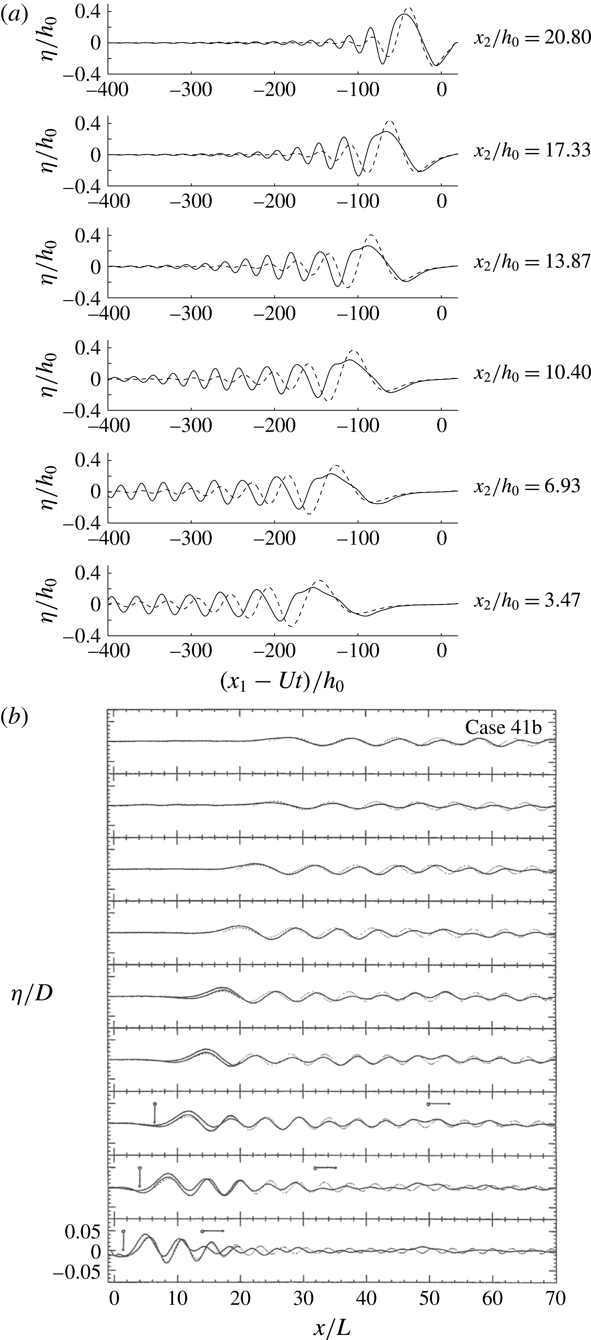
Comparison between the present calculations and Tulin et al.’s case 41b;
 $Fr=4.8$
. (a) Present nonlinear (——) and linear (– – –) downstream wave cuts at transverse distances from the ship track from
 $x_{2}/h_{0}=3.47$
to
 $x_{2}/h_{0}=20.80$
with increments
 $\unicode[STIX]{x0394}x_{2}/h_{0}=3.47$
; present ship model. (b) Reproduction of Tulin et al. (Reference Tulin, Yao and Wang2000, figure 10(a)); half prolate spheroid with radius
 $D$
at mid-section and length
 $L=D/0.097$
,
 $D/h_{0}=0.78$
and same lateral increment between wave cuts.

The ship in the present observations and numerical calculations has a length of
 $l_{0}/h_{0}=29.4$
and average sectional area of
 $3.46h_{0}^{2}$
. Both are 3–4 times larger compared with Tulin et al.’s cases. The ship volume relative to the pycnocline depth cubed is more than 10 times larger compared with the models used by Tulin et al. Thus, the internal wave wake is also much stronger in our case where nonlinear effects are essential, both in the field observation and in the numerics. The opposite is true for the cases considered by Tulin et al. where the wave wake is well within the linear regime. A direct comparison with Tulin et al.’s case 41b for
 $Fr=4.8$
shows that their downstream elevations
 $\unicode[STIX]{x1D702}/D$
are in the range between
 $+0.04$
and
 $-0.03$
, which means that
 $\unicode[STIX]{x1D702}/h_{0}\sim +0.03$
to
 $-0.025$
, see figure 16(b), while in our computations, for the relatively much larger ship, the downstream relative elevation is more than 10 times larger, with
 $\unicode[STIX]{x1D702}/h_{0}$
in the range between
 $+0.4$
and
 $-0.3$
, where also the effect of nonlinearity is very important; see figure 16(a). We note that in Tulin et al.’s case 41b the leading wave trough is absent (their figures 9a, 10a), while in our calculations it is always present, even for the ship models of small draught; see our figures 6 and 14. In the observation, the signature of the leading wave slope, moving faster than the linear long-wave speed, is observed and calculated. This is what defines the opening angle in the observation. This is not reported by Tulin et al. at all.
Tulin et al.’s case 25c has
 $Fr=6.5$
and
 $D/h_{0}=1.28$
(and
 $h_{0}/D=0.78$
). These parameters correspond to the speed and draught of the ship in the present observation, while, however, Tulin et al.’s model has a relative volume that is 10 times smaller compared with the ship described in our paper. Their calculations of the far-field wave elevations shown in their figure 10(b) are in the range
 $\unicode[STIX]{x1D702}/D\sim \pm 0.025$
(
 $\unicode[STIX]{x1D702}/h_{0}\sim \pm 0.03$
) at an off-track distance of
 $x_{2}/D=40.35$
(
 $x_{2}/h_{0}=51.65$
). For comparison, our nonlinear calculations in figure 6(c) are approximately five times larger, while the linear calculations in figure 6(d) are seven times larger, at a similar off-track distance. At the off-track position of
 $x_{2}/h_{0}=91.6$
our nonlinearly calculated and observed trough excursions are
 ${\sim}0.1h_{0}$
, and the linearly calculated troughs are
 ${\sim}0.15h_{0}$
, much greater than in Tulin et al. It is evident that the cases investigated by Tulin et al. are well within the linear range, since the nonlinear correction to the interfacial elevations
 $\unicode[STIX]{x1D702}/h_{0}$
is tiny. Finally, the comparisons with the results in Tulin et al. (Reference Tulin, Yao and Wang2000) show that the nonlinearity of the dead water wake depends on several parameters, including the relative ship draught
 $d_{0}/h_{0}$
and the relative ship volume
 $V_{0}/h_{0}^{3}$
, where the effect of nonlinearity is measured by the interfacial excursions relative to the average pycnocline depth
 $h_{0}$
.
6 Conclusions
Properties of ship-generated internal wave wakes, including the wave amplitudes, induced surface currents and shear rate, as well as the resistance force, are analysed. This is done by means of a strongly nonlinear two-layer model in three dimensions with comparison with field observations and linear calculations. The ship speed is supercritical in the range
 $Fr=U/c_{0}\sim 4{-}12$
, where
 $U$
denotes the ship speed and
 $c_{0}$
is the linear internal long-wave speed. The complex ship geometry is accounted for. The degree of nonlinearity is determined by the ratio between the ship draught (
 $d_{0}$
) and the average depth of the pycnocline (
 $h_{0}$
) and is explored in the range
 $d_{0}/h_{0}\sim 0.1{-}1.2$
. The relevance of the two-layer calculations to the field conditions, where the pycnocline thickness is small or moderately finite, can be justified by existing laboratory measurements (e.g. Grue et al.
Reference Grue, Jensen, Rusås and Sveen1999) and calculations accounting for the continuous density variation (e.g. Fructus & Grue Reference Fructus and Grue2004).
Notable differences between the nonlinear and linear representations of the local flow at the ship as well as in the wave wake are found. The r.m.s. value of the difference between the nonlinear and linear interfacial elevations divided by the r.m.s. value of the nonlinear elevation is found to grow linearly with
 $d_{0}/h_{0}$
. This r.m.s. ratio becomes unity, meaning that the error is 100 %, for
 $d_{0}/h_{0}\sim 1$
and Froude number
 $Fr\sim 4{-}6.6$
. The relative error reduces with increasing Froude number. Calculations for
 $d_{0}/h_{0}\sim 1$
show that the amplitude of the far downstream waves is overpredicted by up to 50 % by the linear method. The nonlinear trough amplitudes decay algebraically in the lateral coordinate with decay exponents in the range 0.16–0.61, where the first four waves are investigated. The first linear trough amplitude is much smaller than the nonlinear one. The second linear trough amplitude is much larger than the nonlinear one, however. The third and fourth linear trough amplitudes grow with the lateral coordinate when this is moderate, up to a maximum that is up to 50 % larger than the corresponding nonlinear amplitudes, and then exhibit a decay in the lateral coordinate. The nonlinear leading trough is systematically somewhat ahead of the classical asymptotic pattern originating from a point disturbance for
 $Fr=4$
, while the succeeding troughs are behind the asymptotic pattern. For the larger Froude numbers of
 $Fr=6.6$
and 12, the nonlinear and asymptotic troughs are rather close, however. The nonlinear internal wave resistance compares with the frictional force for
 $Fr\sim 4{-}6$
, and exceeds the surface wave resistance and increases by 40 % the total drag on an observed ship moving at
 $Fr=6.6$
. A linear force prediction is useless for ship draughts comparable to the depth of the pycnocline.
The calculations are compared with a set of field observations of the internal wave wake of a 221 m long cargo ship of dead weight 43 000 tonnes moving with speed
 $6.6~\text{m}~\text{s}^{-1}$
along a Canadian fjord. The reference length and speed of the two-layer model are determined from the midlevel and density jump of the pycnocline of the sea. In the observations, three prominent beams (waves) of 1–2 m isopycnal displacement riding on the pycnocline were measured, at an off-track distance of approximately 700 m. The calculated phase speeds of the second and third waves fit very well to those observed in the Canadian fjord, while the leading wave in the observation moves at a slightly supercritical speed. The leading slope of the nonlinearly calculated surface velocity moving 7 % ahead of the leading trough may provide some explanation of the observation, where a linear calculation is inferior. The nonlinear computations obtained a wave train of eight waves of height 1.5 m at a similar lateral position, where the excursions fit very well to the field observation. Linear calculations gave a train of four waves of height 2.3 m, however, overpredicting the amplitude. By the calculations we also evaluate the surface velocity and strain rate of the wave wake relevant to one of the ships in the Loch Linnhe experiment, where in particular the strain rates show excellent comparison between the calculations and measurements published in Watson et al. (Reference Watson, Chapman and Apel1992). The linear predictions are quite erroneous. Through comparison with the results in Tulin et al. (Reference Tulin, Yao and Wang2000) it is evident that the nonlinearity of the dead water wake depends on several parameters, including the relative ship draught
 $d_{0}/h_{0}$
and the relative ship volume
 $V_{0}/h_{0}^{3}$
(where
 $h_{0}$
is the average pycnocline depth).
Acknowledgement
This research was initiated at the Conference on Nonlinear Effects in Internal Waves, Cornell University, USA, 8–14 June 2014. J.G. was funded by the Research Council of Norway, NFR191204/V30.
Supplementary material
Supplementary material is available at http://dx.doi.org/10.1017/jfm.2016.518.
Appendix A. Background conditions in the Saguenay Fjord
In the field observations (§ 4), the density field was inferred from the mooring temperature chain using a second-order polynomial fit relating temperature to salinity from 13 CTD profiles collected at various places around the bay between 20:05 and 23:54 UTC (i.e. after the internal wake event) on 13 June (not shown). There is a certain scatter in the data cloud, such that inferring salinity, and thus density, from the temperature measurements alone is accurate to within
 $\pm 0.6~\text{kg}~\text{m}^{-3}$
. Relative to the density jump across the pycnocline of approximately
 $\unicode[STIX]{x0394}\unicode[STIX]{x1D70C}=15~\text{kg}~\text{m}^{-3}$
the relative error introduced is approximately 4 %. One CTD cast was obtained close to the mooring at 20 : 30 UTC (see figure 9 for the position), i.e. after the passage of the ship internal wake, and is shown in figure 10(a) for comparison with the density inferred from the thermistor chain.
The background density structure is typical for this subarctic fjord, with a thin brackish surface layer overlying a thick salty bottom layer. These two layers are separated by a 5 m thick pycnocline located between 5 and 10 m and characterized with buoyancy frequency squared:
 $$\begin{eqnarray}N_{pyc}^{2}=-\frac{g}{\unicode[STIX]{x1D70C}_{0}}\frac{\unicode[STIX]{x2202}\unicode[STIX]{x1D70C}}{\unicode[STIX]{x2202}y}=0.019\pm 0.009~~\text{s}^{-2},\end{eqnarray}$$
where
 $y$
is the vertical axis (positive upward),
 $g=9.81~\text{m}~\text{s}^{-2}$
is the gravitational acceleration and
 $\unicode[STIX]{x1D70C}_{0}=1020~\text{kg}~\text{m}^{-3}$
is a reference density. This corresponds to a buoyancy period of
 $\unicode[STIX]{x1D70F}=2\unicode[STIX]{x03C0}/N=45~\text{s}$
. In terms of
 $N^{2}$
, this background stratification is approximately 25 times greater than the stratification measured in the same area in early July 2007 by Bourgault et al. (Reference Bourgault, Janes and Galbraith2011). They reported
 $N^{2}=7.8\times 10^{-4}~\text{s}^{-2}$
.
The background currents are complex and vertically sheared throughout the water column. The maximum shear layer coincides with the pycnocline (between 5 and 10 m) and is characterized with shear squared, calculated at 3.5 m resolution to match the thermistor vertical spacing:
 $$\begin{eqnarray}S_{pyc}^{2}=\left(\frac{\unicode[STIX]{x2202}\bar{u}}{\unicode[STIX]{x2202}y}\right)^{2}+\left(\frac{\unicode[STIX]{x2202}\bar{v}}{\unicode[STIX]{x2202}y}\right)^{2}=0.006\pm 0.002~\text{s}^{-2},\end{eqnarray}$$
where
 $\bar{u}$
and
 $\bar{v}$
are 15 min averages taken between 18:50 and 19:05 of the eastward and northward velocity component respectively. The pycnocline is therefore characterized with a Richardson number
 $\mathit{Ri}_{pyc}\equiv N_{pyc}^{2}/S_{pyc}^{2}$
between 1 and 7.
It should be noted that the circulation in the bay is quite complex, with the presence of multiple eddies of various sizes and rotational directions, as seen in movies of the sea-surface patterns. The currents at the mooring location may therefore not be representative of the currents in the middle of the channel along the ship track where the internal wake was generated. A close inspection of the movie of the georectified images suggests that the ship may have been steaming against a surface current such that her speed over the surface water may have been higher than the speed over ground
 $U_{ais}$
presented above. However, since the background currents are strongly vertically sheared (figure 10
b) the surface current alone may not either be representative of the sub-surface currents at the depth where the internal wake was generated and elsewhere along the wave propagation, where the currents slowly modify the wave propagation speed. For these reasons of strong lateral and vertical heterogeneity of the currents, it is difficult to determine the background currents of the fjord precisely. The best that can be done is to add an additional uncertainty of approximately
 $0.2~\text{m}~\text{s}^{-1}$
to the current values measured at the mooring at that time (figure 10
b). In other words, this uncertainty indicates that the currents along the ship trace may have been in any direction, with their range assumed to be comparable to the range recorded at the mooring.
Appendix B. Dispersion relations: two- and three-layer fluids
The dispersion relation for a two-layer fluid, with an upper layer of constant density
 $\unicode[STIX]{x1D70C}_{0}$
and depth of
 $h_{0}$
at rest, and a lower layer of constant density
 $\unicode[STIX]{x1D70C}_{1}$
and depth
 $h_{1}$
at rest, see figure 10(d), reads (see Phillips Reference Phillips1966, p. 169; Grue Reference Grue2015a
, equation (3.7))
 $$\begin{eqnarray}\displaystyle (ck_{1})^{2}=g^{\prime }k_{1}/((\unicode[STIX]{x1D70C}_{0}/\unicode[STIX]{x1D70C}_{1})\coth (k_{1}h_{0})+\coth (k_{1}h_{1})), & & \displaystyle\end{eqnarray}$$
where
 $k_{1}$
denotes the wavenumber and
 $c(k_{1})$
the wave speed. The linear long-wave speed obtained for
 $k_{1}\rightarrow 0$
is given in the main text below (2.1). The two-layer model is compared with a three-layer model. In the latter, a mixed upper layer of constant density
 $\unicode[STIX]{x1D70C}_{0}$
and depth
 $H_{0}$
is separated from a mixed lower layer of density
 $\unicode[STIX]{x1D70C}_{1}$
and depth
 $H_{1}$
by a pycnocline of thickness
 $\unicode[STIX]{x1D6FF}$
and constant buoyancy frequency
 $N_{0}$
; see figure 10(c). The dispersion relation becomes (see Fructus & Grue Reference Fructus and Grue2004, equation (4.2))
 $$\begin{eqnarray}\displaystyle K_{\unicode[STIX]{x1D6FF}}^{2}-k_{1}[\coth (k_{1}H_{0})+\coth (k_{1}H_{1})]K_{\unicode[STIX]{x1D6FF}}\cot (K_{\unicode[STIX]{x1D6FF}}\unicode[STIX]{x1D6FF})-k_{1}^{2}\coth (k_{1}H_{0})\coth (k_{1}H_{1})=0, & & \displaystyle\end{eqnarray}$$
where
 $K_{\unicode[STIX]{x1D6FF}}=\sqrt{N_{0}^{2}/c^{2}-k_{1}^{2}}$
. The limit
 $k_{1}\rightarrow 0$
of (B 2) obtains the linear long-wave speed of the three-layer fluid by
 $Y=N_{0}\unicode[STIX]{x1D6FF}/c_{0}^{3lay}$
, where
 $Y$
is the solution of
 $Y^{2}-(\unicode[STIX]{x1D6FF}/H_{0}+\unicode[STIX]{x1D6FF}/H_{1})Y\cot (Y)-\unicode[STIX]{x1D6FF}^{2}/(H_{0}H_{1})=0.$
The wave phase speed
 $c(k_{1})/c_{0}$
and group velocity
 $c_{g}(k_{1})/c_{0}$
for the two- and three-layer fluids show small to moderate differences for
 $k_{1}h_{0}$
up to 0.7 (figure 13).
Appendix C. Asymptotic wave wake pattern
The wave patterns obtained for the two- and three-layer fluids are compared with the nonlinear interfacial calculations. The constant wave phase is given by
 $k_{1}x_{1}+k_{2}x_{2}-\unicode[STIX]{x1D714}t=k(x_{1}\cos \unicode[STIX]{x1D6FD}_{0}+x_{2}\sin \unicode[STIX]{x1D6FD}_{0}-ct)=\unicode[STIX]{x1D712}_{0}$
, where
 $(k_{1},k_{2})$
denotes the horizontal wavenumber vector,
 $k=\sqrt{k_{1}^{2}+k_{2}^{2}}$
,
 $\unicode[STIX]{x1D6FD}_{0}$
is the wave angle with respect to the
 $x_{1}$
-axis,
 $\unicode[STIX]{x1D712}_{0}=0,-2\unicode[STIX]{x03C0},-4\unicode[STIX]{x03C0}\ldots$
are the constant phases,
 $\unicode[STIX]{x1D714}$
is the wave frequency and
 $t$
is time. Obtaining the gradient
 $(\unicode[STIX]{x2202}/\unicode[STIX]{x2202}k_{1},\unicode[STIX]{x2202}/\unicode[STIX]{x2202}k_{2})$
of the phase function gives
 $x_{1}-c_{g}\cos \unicode[STIX]{x1D6FD}_{0}\,t=0$
,
 $x_{2}-c_{g}\sin \unicode[STIX]{x1D6FD}_{0}\,t=0$
, where
 $c_{g}=\unicode[STIX]{x2202}\unicode[STIX]{x1D714}/\unicode[STIX]{x2202}k$
denotes the group velocity and where
 $\unicode[STIX]{x2202}c/\unicode[STIX]{x2202}k_{1}=c_{g}\cos \unicode[STIX]{x1D6FD}_{0}$
and
 $\unicode[STIX]{x2202}c/\unicode[STIX]{x2202}k_{2}=c_{g}\sin \unicode[STIX]{x1D6FD}_{0}$
are used. The wave angle is determined using the fact that the wave motion, in a frame of reference moving with the ship speed
 $U$
, is stationary. A lateral current
 $-V$
along the
 $x_{2}$
-axis is accounted for. This gives
 $$\begin{eqnarray}\displaystyle Uk_{1}+Vk_{2}-\unicode[STIX]{x1D714}=k(U\cos \unicode[STIX]{x1D6FD}_{0}+V\sin \unicode[STIX]{x1D6FD}_{0}-c)=0. & & \displaystyle\end{eqnarray}$$
Combination of the equations gives
 $$\begin{eqnarray}\displaystyle & \displaystyle (x_{2}-Vt)\,k\,(c-c_{g})=-\unicode[STIX]{x1D712}_{0}c_{g}\sqrt{1-c^{2}/U^{2}}+\unicode[STIX]{x1D712}_{0}V(1-cc_{g}/U^{2}), & \displaystyle\end{eqnarray}$$
 $$\begin{eqnarray}\displaystyle & \displaystyle (x_{1}-Ut)\,k\,(c-c_{g})=\unicode[STIX]{x1D712}_{0}U(1-cc_{g}/U^{2})+\unicode[STIX]{x1D712}_{0}c_{g}(V/U)\sqrt{1-c^{2}/U^{2}}. & \displaystyle\end{eqnarray}$$
Equations (C 2)–(C 3) account for a lateral current
 $V$
that is assumed to be small compared with
 $U$
((C 1) is exact) and generalize the equations derived by Keller & Munk (Reference Keller and Munk1970, equations (12)–(13)) for the internal ship wave wake pattern.
Appendix D. Expressions for
 $W_{I}^{(3)}$
and
$V_{I}^{(3)}$


The normal velocities
 $W_{I},V_{I}$
defined in (2.2) are obtained by a set of integral equations solving the Laplace equation in fluids 0 and 1; see Grue (Reference Grue2015a
,Reference Grue
b
). Solutions to these equations are obtained by the method of successive approximations, where
 $W_{I}=W_{I}^{(1)}+W_{I}^{(2)}+W_{I}^{(3)}+\ldots$
and
 $V_{I}=V_{I}^{(1)}+V_{I}^{(2)}+V_{I}^{(3)}+\ldots$
; see § 2. The functions
 $W_{I}^{(1)}$
and
 $W_{I}^{(2)}$
are obtained in (2.4)–(2.5), and
 $V_{I}^{(1)}$
and
 $V_{I}^{(2)}$
are obtained in (2.6)–(2.7). The function
 $W_{I}^{(3)}$
is obtained by
 $$\begin{eqnarray}\displaystyle {\hat{W}}_{I}^{(3)} & = & \displaystyle \frac{k}{1+e_{0}}({\hat{W}}_{I}^{(3,1)}+{\hat{W}}_{I}^{(3,2)}+{\hat{W}}_{I}^{(3,3)}+{\hat{W}}_{I}^{(3,4)}),\end{eqnarray}$$
 $$\begin{eqnarray}\displaystyle {\hat{W}}_{I}^{(3,1)} & = & \displaystyle -e_{0}{\mathcal{F}}[\unicode[STIX]{x1D702}(W_{I}-W_{I}^{(1)})]-{\mathcal{F}}\{\unicode[STIX]{x1D702}{\mathcal{F}}^{-1}[e_{0}({\hat{W}}_{I}-{\hat{W}}_{I}^{(1)})]\},\end{eqnarray}$$
 $$\begin{eqnarray}\displaystyle {\hat{W}}_{I}^{(3,2)} & = & \displaystyle -{\textstyle \frac{1}{2}}k(1+e_{0}){\mathcal{F}}(\unicode[STIX]{x1D702}^{2}W_{I})+{\mathcal{F}}\{\unicode[STIX]{x1D702}{\mathcal{F}}^{-1}[k(1-e_{0}){\mathcal{F}}(\unicode[STIX]{x1D702}W_{I})]\}\nonumber\\ \displaystyle & & \displaystyle -\,{\textstyle \frac{1}{2}}{\mathcal{F}}\{\unicode[STIX]{x1D702}^{2}{\mathcal{F}}^{-1}[k(1+e_{0})\hat{W_{I}}]\},\end{eqnarray}$$
 $$\begin{eqnarray}\displaystyle {\hat{W}}_{I}^{(3,3)} & = & \displaystyle -{\textstyle \frac{1}{2}}e_{0}\text{i}\boldsymbol{k}\boldsymbol{\cdot }{\mathcal{F}}(\unicode[STIX]{x1D702}^{2}\unicode[STIX]{x1D735}_{H}\unicode[STIX]{x1D719}_{0I})-{\mathcal{F}}\{\unicode[STIX]{x1D702}{\mathcal{F}}^{-1}[e_{0}\text{i}\boldsymbol{k}\boldsymbol{\cdot }{\mathcal{F}}(\unicode[STIX]{x1D702}\unicode[STIX]{x1D735}_{H}\unicode[STIX]{x1D719}_{0I})]\}\nonumber\\ \displaystyle & & \displaystyle +\,{\textstyle \frac{1}{2}}{\mathcal{F}}[\unicode[STIX]{x1D702}^{2}{\mathcal{F}}^{-1}(e_{0}k^{2}\unicode[STIX]{x1D719}_{0I})],\end{eqnarray}$$
 $$\begin{eqnarray}\displaystyle {\hat{W}}^{(3,4)} & = & \displaystyle {\mathcal{F}}(\unicode[STIX]{x1D702}^{2}{\mathcal{F}}^{-1}[k\sqrt{e_{0}}{\hat{W}}_{F}])+k\sqrt{e_{0}}{\mathcal{F}}(\unicode[STIX]{x1D6FD}^{2}W_{F})\nonumber\\ \displaystyle & & \displaystyle -\,{\mathcal{F}}(\unicode[STIX]{x1D702}{\mathcal{F}}^{-1}[2\sqrt{e_{0}}\text{i}\boldsymbol{k}\boldsymbol{\cdot }{\mathcal{F}}(\unicode[STIX]{x1D6FD}\unicode[STIX]{x1D735}_{H}\unicode[STIX]{x1D719}_{0F})]),\end{eqnarray}$$
where a hat denotes Fourier transform and
 $e_{0}=\text{e}^{-2kh_{0}}$
. The function
 $V_{I}^{(3)}$
is given by
 $$\begin{eqnarray}\displaystyle \hat{V_{I}}^{(3)} & = & \displaystyle \frac{k}{1+e_{1}}(\hat{V_{I}}^{(3,1)}+\hat{V_{I}}^{(3,2)}+\hat{V_{I}}^{(3,3)}),\end{eqnarray}$$
 $$\begin{eqnarray}\displaystyle \hat{V_{I}}^{(3,1)} & = & \displaystyle e_{1}{\mathcal{F}}[\unicode[STIX]{x1D702}(V_{I}-V_{I}^{(1)})]+{\mathcal{F}}\{\unicode[STIX]{x1D702}{\mathcal{F}}^{-1}[e_{1}(\hat{V_{I}}-\hat{V}_{I}^{(1)})]\},\end{eqnarray}$$
 $$\begin{eqnarray}\displaystyle \hat{V_{I}}^{(3,2)} & = & \displaystyle -{\textstyle \frac{1}{2}}k(1+e_{1}){\mathcal{F}}(\unicode[STIX]{x1D702}^{2}V_{I})+{\mathcal{F}}\{\unicode[STIX]{x1D702}{\mathcal{F}}^{-1}[k(1-e_{1}){\mathcal{F}}(\unicode[STIX]{x1D702}V_{I})]\}\nonumber\\ \displaystyle & & \displaystyle -\,{\textstyle \frac{1}{2}}{\mathcal{F}}\{\unicode[STIX]{x1D702}^{2}{\mathcal{F}}^{-1}[k(1+e_{1})\hat{V_{I}}]\},\end{eqnarray}$$
 $$\begin{eqnarray}\displaystyle \hat{V_{I}}^{(3,3)} & = & \displaystyle {\textstyle \frac{1}{2}}e_{1}\text{i}\boldsymbol{k}\boldsymbol{\cdot }{\mathcal{F}}(\unicode[STIX]{x1D702}^{2}\unicode[STIX]{x1D735}_{H}\unicode[STIX]{x1D719}_{1I})+{\mathcal{F}}\{\unicode[STIX]{x1D702}{\mathcal{F}}^{-1}[e_{1}\text{i}\boldsymbol{k}\boldsymbol{\cdot }{\mathcal{F}}(\unicode[STIX]{x1D702}\unicode[STIX]{x1D735}_{H}\unicode[STIX]{x1D719}_{1I})]\}\nonumber\\ \displaystyle & & \displaystyle -{\textstyle \frac{1}{2}}{\mathcal{F}}[\unicode[STIX]{x1D702}^{2}{\mathcal{F}}^{-1}(e_{1}k^{2}\hat{\unicode[STIX]{x1D719}}_{1I})],\end{eqnarray}$$
where
 $e_{1}=\text{e}^{-2kh_{1}}$
.