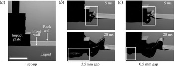
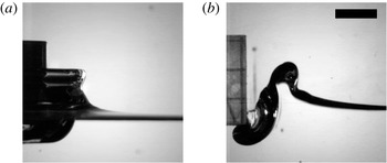
1 Introduction
1.1 Motivation and problem background
While research on water impact was originally motivated by landing on sea (von Karman Reference von Karman1929), its more general practical importance, ranging from the slamming of ships to the impact of water waves on coastal structures, has been recognized in a number of review articles from Szebehely (Reference Szebehely1960) to Peseux, Gornet & Donguy (Reference Peseux, Gornet and Donguy2005). While other impact phenomena – impacts of liquid drops, solid spheres, wedges, cones and disks – share the same qualitative features, we will focus on the flat rectangular plate impact. Among the variety of impacts between liquids and solids, it represents the utmost classical case where the complexities of other configurations, e.g. moving contact lines, are absent and therefore one can focus on the key aspects of the phenomena – abrupt changes in the fluid flow and free surface (ejecta) – considered in the present manuscript.
Under the condition when the impact velocity
 $V_{0}$
is much lower than the speed of sound
 $c_{0}$
in the liquid phase of density
 $\unicode[STIX]{x1D70C}$
, the acoustic wave carries away energy that is negligible not only compared to the kinetic energy of the liquid added mass
 $\unicode[STIX]{x03C0}w^{2}\unicode[STIX]{x1D70C}\,V_{0}^{2}/2$
for the plate of half-width
 $w$
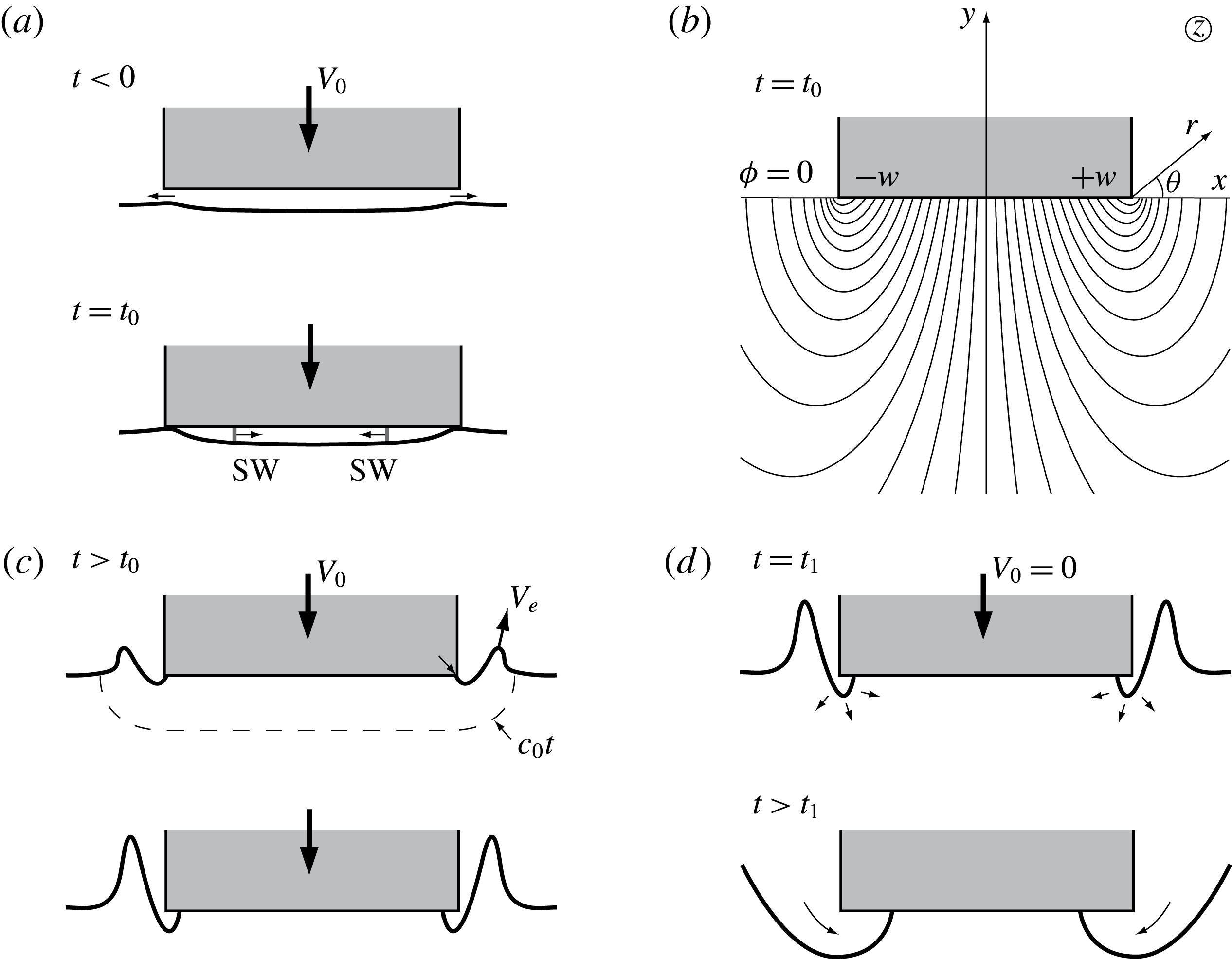
, but also to the total (kinetic and potential due to gravity and surface tension) energy of the liquid ejected due to splash. Hence, in the initial acoustic stage the flow quickly relaxes to the incompressible solution, i.e. the hydraulic stage we are going to focus on here. The incompressible inviscid solution right after the impact of the plate on a semi-infinite body of quiescent liquid shown in figure 1(b) is well-known (Batchelor Reference Batchelor1967). Since physically for
 $t\rightarrow +0$
the sudden acceleration of the liquid from rest to a finite velocity in a step-wise manner
 $\boldsymbol{v}\sim H(t)$
can be balanced only by the pressure gradient (impulse)
 $p\sim H^{\prime }(t)=\unicode[STIX]{x1D6FF}_{D}(t)$
and not by liquid viscosity and inertia (and gravity), the Navier–Stokes equations (NSEs) reduce to
 $\unicode[STIX]{x2202}\boldsymbol{v}/\unicode[STIX]{x2202}t=-\unicode[STIX]{x1D735}p/\unicode[STIX]{x1D70C}$
, which together with the incompressibility condition
 $\unicode[STIX]{x1D735}\boldsymbol{\cdot }\boldsymbol{v}=0$
lead to the existence of a velocity potential
 $\unicode[STIX]{x1D719}$
. The latter is a solution of the Hilbert problem on the lower half-plane
 $\mathbb{H}^{-}$
for a bounded harmonic function
 $\unicode[STIX]{x1D719}$
constructed from the knowledge of its values and its normal derivatives at the boundary (Mikhlin Reference Mikhlin1964):
 $$\begin{eqnarray}\displaystyle \unicode[STIX]{x0394}\unicode[STIX]{x1D719} & = & \displaystyle 0,\quad (x,y)\in \mathbb{H}^{-},\end{eqnarray}$$
 $$\begin{eqnarray}\displaystyle y=0:\unicode[STIX]{x1D719}_{y} & = & \displaystyle -V_{0},x\in [-w,w];\unicode[STIX]{x1D719}=0,x\notin [-w,w].\end{eqnarray}$$
 $f$
right after impact:
 $$\begin{eqnarray}f(z)=\unicode[STIX]{x1D719}+\text{i}\unicode[STIX]{x1D713}=\text{i}V_{0}(z-\sqrt{z^{2}-w^{2}}),\quad \text{where }z=x+\text{i}y,\end{eqnarray}$$
with the streamlines
 $\unicode[STIX]{x1D713}$
shown in figure 1(b). A point to make about (1.2) is that the ideal fluid flow is set instantaneously and is thereafter steady for negligible penetration depths at
 $t>0$
, except for the near-edge velocity field and the ejecta, which are evolving, as illustrated in figure 1(c).
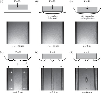
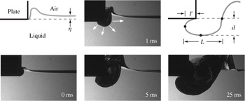
Key stages of water impact: (a) air entrapment, (b) establishing flow field
 $\unicode[STIX]{x1D713}(x,y)$
, (c) ejecta formation, (d) air pocketing.

The picture would be incomplete without other key features of a realistic water impact at finite penetration depth and in the presence of atmosphere: air entrapment due to a non-zero initial separation from the water surface (since for all the air to be forced out the air escape velocity would have be infinite, which is physically impossible), cf. figure 1(a), and air pocketing due to a sudden halt at some finite depth of penetration, e.g. due to buoyancy in the case of a free-falling body or intentional deceleration of a landing aircraft with external forces to avoid submerging upon impact, shown in figure 1(d). This sudden halt or deceleration of the body upon impact has usually been omitted in previous works (Yakimov Reference Yakimov1973; Chuang Reference Chuang1966), but represents an integral part of the impact phenomena.
1.2 Key questions
Of particular interest here are the aspects of the flat plate impact phenomena usually neglected in previous studies, which can be investigated in the present paper by scaled experiments, namely realistic effects such as viscosity and surface tension influencing the physics of impact. The need to look at these effects can be understood from the inviscid potential flow solution (1.2), which raises several issues near the plate edge. First, the velocity field
 $u+\text{i}\,v=\overline{\text{d}f/\text{d}z}$
is singular there:
 $$\begin{eqnarray}\boldsymbol{v}=(u,v)=a/\sqrt{2r}[-\sin (\unicode[STIX]{x1D703}/2),\cos (\unicode[STIX]{x1D703}/2)],\quad \text{ where }r\ll w\text{ and }a=V_{0}\sqrt{w},\end{eqnarray}$$
where
 $u$
and
 $v$
are
 $x$
- and
 $y$
-velocity components, respectively, and
 $(r,\unicode[STIX]{x1D703})$
the polar system positioned at the plate edge, indicated in figure 1(b). As can be gleaned from the streamlines in that figure, the fluid makes a right angle turn around the plate edge with the vertical velocity component being unbounded at the fluid interface as
 $r\rightarrow 0$
and hence the question arises as to how neglected viscosity and surface tension regularize this singularity.
The velocity divergence (1.3) also brings the second issue: the fluid interface must instantly stretch to infinity, which is non-physical and results from neglecting important physics. For example, surface tension would not permit infinite stretching of the interface as it would require an infinite amount of energy and thus violate energy conservation (Krechetnikov Reference Krechetnikov2014b
), hence invalidating the argument of Iafrati & Korobkin (Reference Iafrati and Korobkin2004) that surface tension can be considered as a second-order effect, i.e. represents a regular perturbation to the flow with zero surface tension. Instead, surface tension
 $\unicode[STIX]{x1D70E}$
is certainly needed to resolve the singularity of infinitely stretched interface, i.e. the limit
 $\unicode[STIX]{x1D70E}\rightarrow 0$
is singular in the sense of perturbation theory. As a remedy to the unbounded velocity field near the plate edge in the inviscid potential approximation, Iafrati & Korobkin (Reference Iafrati and Korobkin2004) suggested imposing the Kutta–Joukowsky (KJ) condition, namely that the flow must leave the plate tangentially, which in turn forces the interface to be tangent to the plate as well. Indeed, if the velocity vector leaves the plate edge tangentially, then
 $v=0$
, but the kinematic boundary condition written in the Cartesian coordinates:
 $$\begin{eqnarray}y=\unicode[STIX]{x1D702}(t,x):~\unicode[STIX]{x1D702}_{t}+u\unicode[STIX]{x1D702}_{x}=v,\end{eqnarray}$$
permits free surface growth in time,
 $\unicode[STIX]{x1D702}_{t}>0$
, if the apparent contact angle is non-zero,
 $\unicode[STIX]{x1D702}_{x}\neq 0$
. However, this entails fluid penetration into the upper half-plane, which in turn implies that the vertical velocity component
 $v$
is non-zero, thus leading to a contradiction.
Third, the absence of an independent length scale near the plate edge motivated the use of the Yakimov (Reference Yakimov1973) scaling near the edge, i.e. that during the initial stage the local flow is self-similar with the ensuing time-stretched variables
 $$\begin{eqnarray}\boldsymbol{v}(r,\unicode[STIX]{x1D703})=t^{-1/3}\widetilde{\boldsymbol{v}}(\widetilde{r},\unicode[STIX]{x1D703}),\quad \widetilde{r}=a^{-2/3}t^{-2/3}r,\end{eqnarray}$$
which was arrived at from the above velocity scaling (1.3) near the plate edge, but, as we will discuss in § 3.5, neither applies in the bulk flow for any Reynolds and Weber numbers nor at the interface for the moderate Reynolds and Weber numbers studied here.
And, lastly, the fourth issue is that the inviscid theory (1.1)–(1.2) was developed under the idealistic assumption that the plate is infinitely thin and penetrated an infinitesimally short distance. Such an assumption is, however, impractical as finite thickness of the impactor is necessary to avoid its deformation, but also makes the impact of a plate initially floating on the liquid surface not an ideal experiment as well due to the menisci always present at the plate edges meaning that the liquid surface is initially non-horizontal (see also the discussion in § 3.4). Addressing the above four issues will naturally lead to understanding of the limits of applicability of the inviscid solution (1.2). Also, direct measurements of the free surface profiles will enable us to verify the available theoretical scalings for the ejecta, i.e.
 $y\sim x^{-1/2}$
for an outer surface profile in the inviscid approximation as a simple consequence of (1.3) and
 $y\sim x^{3/2}$
for an inner surface profile in the Stokes regime (Krechetnikov Reference Krechetnikov2014b
), as well as to test self-similarity of the ejecta.
1.3 The idea of experiments and paper outline
To address the above questions, the experimental set-up should be capable of resolving the following key features illustrated in figure 1: (a) at the time instant
 $t_{0}$
sudden impact of a blunt body at finite velocity
 $V_{0}$
accompanied by air trapping; (b) establishment of the flow field in the liquid phase corresponding to the classical solution (1.2); (c) formation of a liquid jet (ejecta) thrown out around the plate edges and abrupt deceleration of the impactor at some finite depth of penetration, which may lead to (d) air pocketing upon sudden stop at the time instant
 $t_{1}$
. The detailed discussion of the physical mechanisms at each of the stages will be given in the context of the respective processes in §§ 3–6.
With the above general understanding, the idea of our experiments is as follows. We considered the problem when the impactor penetrates at constant speed over some shallow depth
 $h$
, so that during the short time of penetration we can compare with the classical theory valid for negligible penetration depth (also assumed in subsequent studies, e.g. Iafrati & Korobkin Reference Iafrati and Korobkin2004), which is of the key interest here (e.g. ejecta formation, KJ condition, Yakimov’s scaling – all these phenomena are tied up to the early times). With the same set-up we also aimed to study the effect of deceleration in the most interesting regime when air pocketing takes place. Hence, given that the four key elements of the story – near the plate edge flow field (§ 3), ejecta formation (§ 4), air entrapment (§ 5) and pocketing (§ 6) – are intertwined, for the sake of continuity they are presented here as a single story.
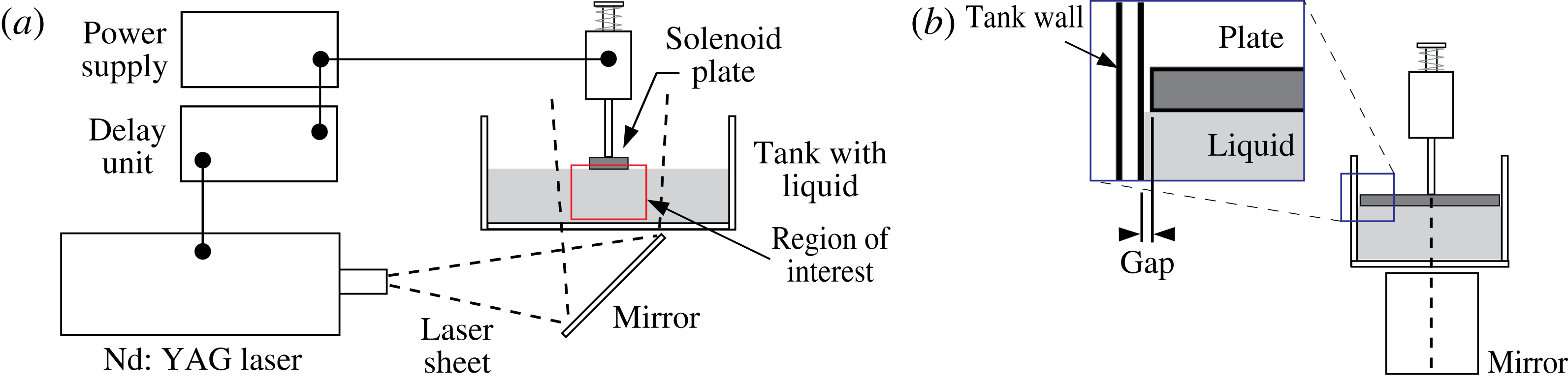
Schematic diagram of the water impact apparatus. (a) The ‘front view’ used for visualization of the flow field and liquid surface (either by particle image velocimetry (PIV) or high-speed camera). The region of interest is typically beneath the plate and near the edges. For imaging the underside of the plate, the laser is not used. Instead, the mirror is rotated toward the camera and the image reflected by the mirror is recorded. (b) The ‘side view’ highlights that the impact plates span nearly the width of the tank to achieve the desired optical access (see the Appendix). Only small gaps (substantially less than the capillary length) are present between the plates and the tank walls.

2 Experimental set-up and procedure
2.1 Impact apparatus hardware
Experiments were carried out with the apparatus sketched in figure 2. Rigid (stainless steel) rectangular plates of a half-width
 $w=5{-}25~\text{mm}$
and total length
 $l=70~\text{mm}$
, with razor-sharp edges machined to
 $0.001~\text{in.}$
accuracy, were attached to the plunger of an electromagnetic solenoid. The travel of the plunger was guided by a Delrin bearing that ran along two polished stainless steel optical posts (not shown in figure 2). The entire solenoid assembly was mounted to a long-travel linear translation stage having a Vernier scale, allowing us to control the depth of impact
 $h$
with reproducible positioning above the liquid surface (
 $\pm 0.05~\text{mm}$
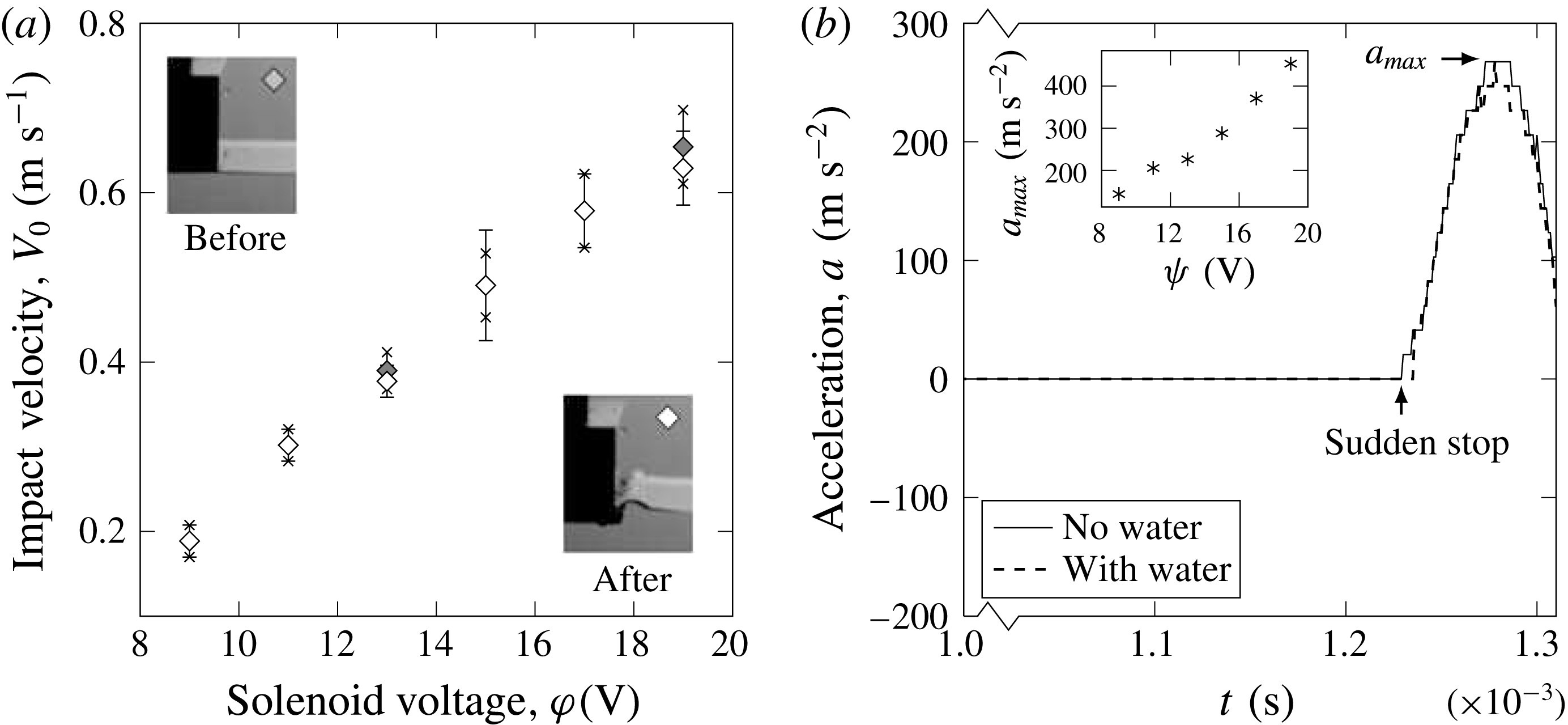
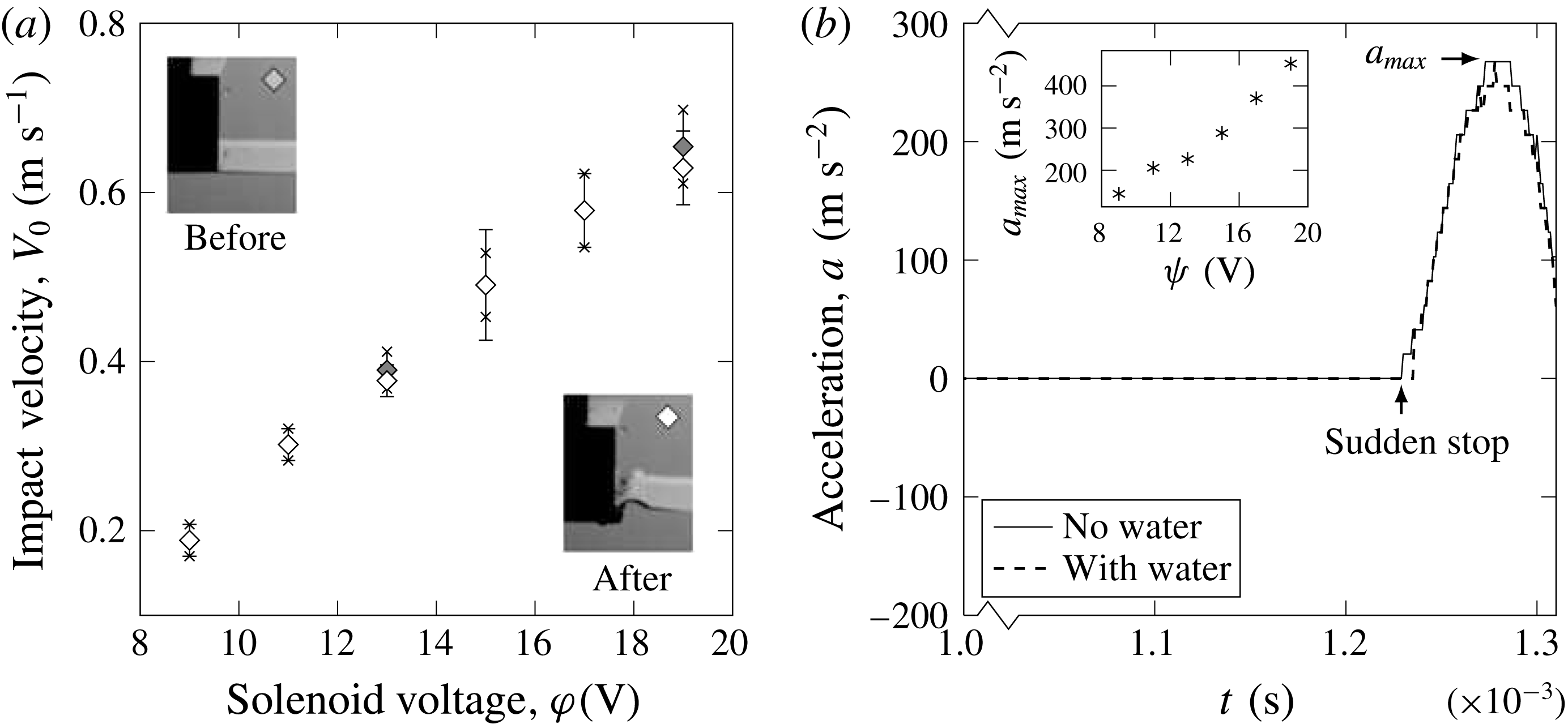
) after cleaning the working liquid off the bottom of the impact plate between each impact event. By adjusting the voltage supplied to the solenoid from a laboratory power supply (GW Instek GPD-3303), the velocity
 $V_{0}$
of the plate at impact could be varied in the range of
 $0.1-1.0~\text{m}~\text{s}^{-1}$
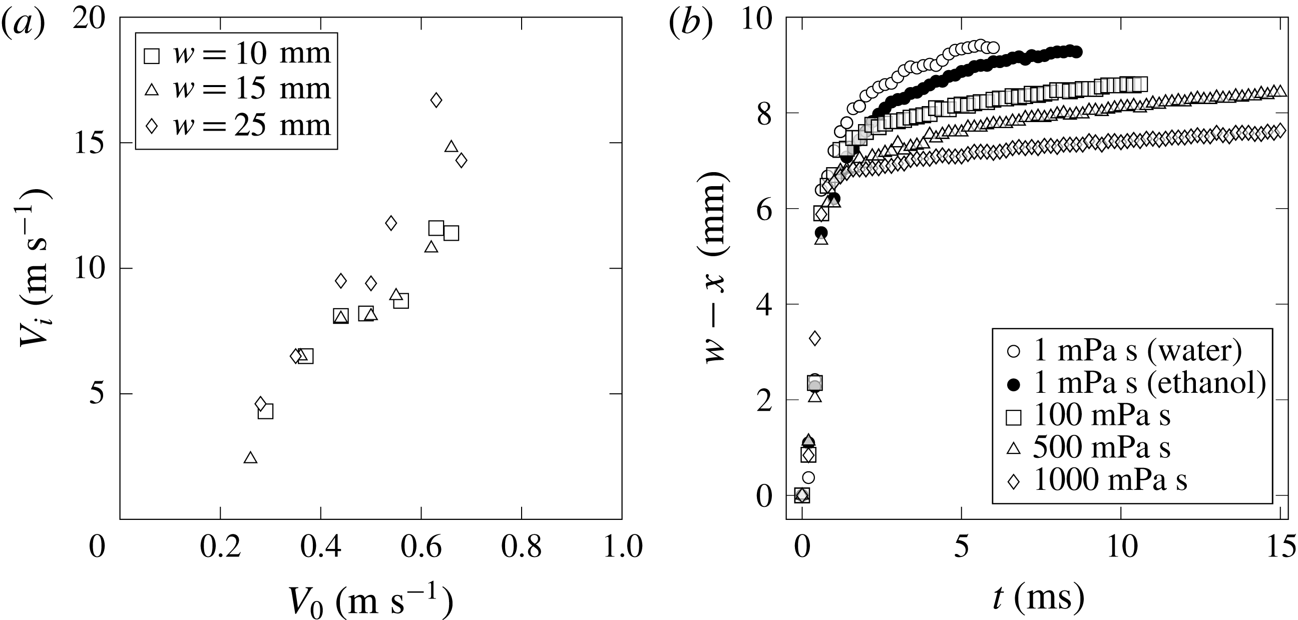
, as shown in figure 3(a). We found that by machining the impact plates of equal weight but varying the half-width
 $w$
, the impact velocity was both repeatable and a sole function of the supplied voltage (figure 3). The use of a solenoid to drive the impact plate has the advantage of ensuring a constant plate velocity during the impact and liquid penetration stages, cf. figure 3(a), as well as an abrupt deceleration comparable in magnitude
 $O(10-100\,g)$
to that in other experiments and realistic impact events (Lewison & Maclean Reference Lewison and Maclean1968; Lin & Shieh Reference Lin and Shieh1997b
; Ermanyuk & Gavrilov Reference Ermanyuk and Gavrilov2011), producing in our situation air pocketing phenomena depicted in figure 1(d). The constancy of the velocity before and during penetration is confirmed from high-speed movies of each impact event, in which a marker located on the plate/plunger is tracked by an image analysis program, and from direct accelerometer measurements in figure 3(b). Constant velocity during impact and penetration is in contrast to experiments where objects fall under their own weight and, depending on the inertia of the object, can be significantly slowed down by the impact event, the drag and buoyancy forces that result. Since the flow quickly relaxes to the incompressible (hydraulic stage) solution, we can justify the (realistic) finite size and depth of the tank, as the reflected acoustic waves do not affect the ejecta formation in view of the insignificant energy associated with such waves. With optical access discussed in the Appendix, our set-up enables us to capture all aspects of an impact event for quantitative analysis. This includes the velocity field beneath the plate and in the vicinity of the plate edge, formation and evolution of the ejecta along with air entrapment during impact and air pocketing after the sudden deceleration of the plate.
Characterization of solenoid velocity and deceleration. (a) Solenoid voltage
 $\unicode[STIX]{x1D711}$
is adjusted to change the impact plate velocity
 $V_{0}$
. Measurements of the plate velocity immediately before and after impact demonstrate that
 $V_{0}$
is constant as also evidenced with the record of acceleration in (b), made with a DeltaTron accelerometer (type 4513 by Brüel and Kjær). All experiments, in which the impact plate is not photographed directly using the high-speed camera (e.g. PIV), involve a procedure of recording a marker on the solenoid plunger to extract the velocity of the impact plate and the time of impact.
It should be mentioned that our apparatus differs from those in recent literature. For example, the set-up in Ermanyuk & Ohkusu (Reference Ermanyuk and Ohkusu2005) and Ermanyuk & Gavrilov (Reference Ermanyuk and Gavrilov2011) is for a free-fall impact of a circular disk, while the set-up in Bergmann et al. (Reference Bergmann, van der Meer, Gekle, van der Bos and Lohse2009) and Peters, van der Meer & Gordillo (Reference Peters, van der Meer and Gordillo2013) is for pulling a circular disk with a linear motor from beneath the tank, i.e. there is a rod which moves through (and hence disturbs) the water surface. In our case, we move the rectangular plate with a solenoid, hitting the water surface which is disturbed only naturally, i.e. first with the displaced air and then with the plate itself. The only instance in the literature in which a plate is abruptly decelerated in the liquid, independent of the hydrodynamic forces on the object, is reported in Huera-Huarte, Jeon & Gharib (Reference Huera-Huarte, Jeon and Gharib2011): the plates in these experiments are stopped by a carrier system guiding the plates well after the significant impact forces of interest have been measured.
2.2 Fluid properties and experimental conditions
In our experiments performed in air at room temperature we can vary the impact speed
 $V_{0}$
, plate half-width
 $w$
and impact depth
 $h$
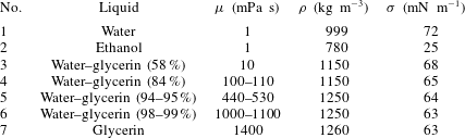
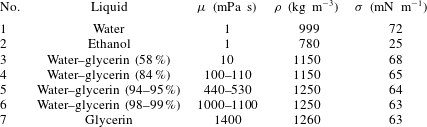
, while the choice of liquid in table 1 sets the density
 $\unicode[STIX]{x1D70C}$
, dynamic viscosity
 $\unicode[STIX]{x1D707}=\unicode[STIX]{x1D70C}\,\unicode[STIX]{x1D708}$
and surface tension
 $\unicode[STIX]{x1D70E}$
. All the liquid solutions were prepared fresh with deionized water to avoid the effects of contamination with surface-active substances and thus guarantee constancy of the surface tension and wettability, although for the relatively high-speed phenomena we study the effects of surface tension varying along the interface should be negligible compared to, say, water wave experiments (Henderson, Segur & Carter Reference Henderson, Segur and Carter2010). Thus, with
 $l$
and
 $h$
fixed, Buckingham’s Pi theorem gives three dimensionless groups relevant to the impact experiments: the Reynolds
 $Re=\unicode[STIX]{x1D70C}\,V_{0}\,w/\unicode[STIX]{x1D707}$
, Weber
 $We=\unicode[STIX]{x1D70C}V_{0}^{2}w/\unicode[STIX]{x1D70E}$
and Froude
 $Fr=V_{0}^{2}/(g\,w)$
numbers. The relative contribution of viscous and surface tension forces can be measured either with the Ohnesorge
 $Oh=\sqrt{We}/Re=\unicode[STIX]{x1D707}/\sqrt{\unicode[STIX]{x1D70C}\,\unicode[STIX]{x1D70E}\,w}$
or Morton
 $Mo=g\,\unicode[STIX]{x1D707}^{4}/\unicode[STIX]{x1D70C}\,\unicode[STIX]{x1D70E}^{3}$
numbers, clearly not independent of
 $Re$
and
 $We$
. For the range of values for
 $V_{0}=0.1-1~\text{m}~\text{s}^{-1}$
and
 $w=5{-}25~\text{mm}$
used in our experiments, and the liquid properties shown in table 1, we find that our range of Reynolds numbers is
 $0.5<Re<25\,000$
. This suggests that viscous effects should only play a significant role for the most viscous fluids tested and for the smallest impact velocities. The corresponding range of Weber number spans
 $1<We<800$
, suggesting that the (global) influence of surface tension will be noticeable at low impact velocities.
Physical properties of liquids used in impact experiments.
Note that since we are interested in the early stages of the water impact, the associated accelerations
 $\unicode[STIX]{x2202}\boldsymbol{v}/\unicode[STIX]{x2202}t$
are considerably higher than gravity, so that the Froude and Morton numbers drop out from most of our analysis, except for the air pocketing study in § 6. Indeed, gravity is neglected in the formulation (1.1) on the ground that the entire flow field is brought into motion simultaneously (due to incompressibility) by the pressure impulse
 $p\sim \unicode[STIX]{x1D6FF}_{D}(t)$
. With the natural non-dimensionalization
 $r\rightarrow w\,r$
,
 $\boldsymbol{v}\rightarrow V_{0}\,\boldsymbol{v}$
,
 $t\rightarrow (w/V_{0})\,t$
and further scaling near the plate edge at early times
 $t\rightarrow \unicode[STIX]{x1D705}\,t$
,
 $r\rightarrow \unicode[STIX]{x1D716}\,r$
,
 $\boldsymbol{v}\rightarrow \unicode[STIX]{x1D6FF}\,\boldsymbol{v}$
(where
 $\unicode[STIX]{x1D705}\ll 1$
,
 $\unicode[STIX]{x1D716}\ll 1$
and
 $\unicode[STIX]{x1D6FF}=\unicode[STIX]{x1D716}^{-1/2}$
per equation (1.3)) all the resulting non-dimensional variables are
 $O(1)$
, the gravity term in the NSEs becomes
 $\unicode[STIX]{x1D716}^{1/2}\unicode[STIX]{x1D705}/Fr$
, from where we conclude that gravity effect is negligible for short times
 $\unicode[STIX]{x1D705}\ll 1$
and distances
 $r\ll 1$
. In dimensional terms, gravity becomes relevant at the times
 $t\geqslant w^{3/2}\,V_{0}^{-1}r^{-1/2}~Fr$
; e.g. for
 $V_{0}=1~\text{m}~\text{s}^{-1}$
,
 $w=1~\text{cm}$
we find
 $t\geqslant O(0.1)~\text{s}$
, which is well beyond the short times of interest for us; close to the edge,
 $r\ll w$
, this minimal time becomes even longer owing to higher fluid acceleration. The irrelevance of gravity at early times has been also recognized in the literature (Iafrati & Korobkin Reference Iafrati and Korobkin2004; Peters et al.
Reference Peters, van der Meer and Gordillo2013).
3 Results: flow field
3.1 Previous efforts
There are few contributions on visualization of the flow field in flat plate impact as the main focus of previous experiments was on loads and, hence, pressure distributions (Chuang Reference Chuang1966). However, the details of the velocity vector field (compared to measurements of scalar functions – pressure or surface elevation) may provide further insights into the physical origin of the pressure peaks and ejecta formation as well as allow one to test various assumptions made in theoretical models, in particular how the singularity near the plate edge is resolved and if there is self-similarity of the velocity field.
Despite the lack of such measurements for flat plate impact, it is worth mentioning earlier attempts at visualizing the velocity field in impact phenomena by Richardson (Reference Richardson1948) on the qualitative flow field around an impacting solid sphere using the Edgerton stroboscope; by Hughes (Reference Hughes1972) also with a stroboscope on quantitative, though scarce and only for one set of impact conditions, measurements of particle paths and total velocity isolines in a wedge impact; and by Lin & Shieh (Reference Lin and Shieh1997a ,Reference Lin and Shieh b ), on the impact of a cylinder, who presented noisy quantitative data as a proof of concept rather than with a goal to study the physics of the phenomena. Also, recently, Nila, Vepa & Paepegem (Reference Nila, Vepa, Vanlanduit and Paepegem2013), Panciroli & Porfiri (Reference Panciroli and Porfiri2013) and Jalalisendi, Zhao & Porfiri (Reference Jalalisendi, Zhao and Porfiri2017) used PIV measurements of the velocity field in the wedge impact to reconstruct pressure and thus infer loads from the NSEs with a Poisson-based solver as a substitute for pressure sensors, which are intrusive.
3.2 Global flow field
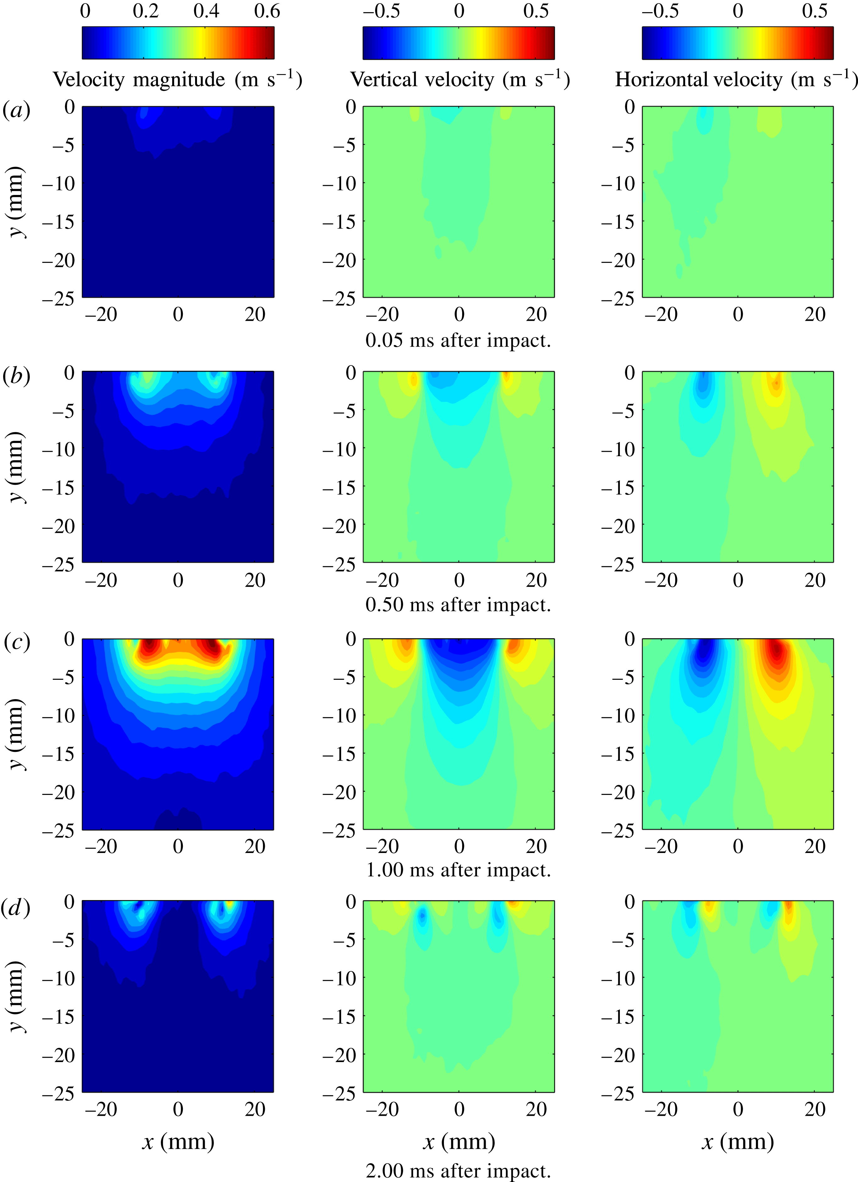
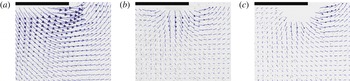
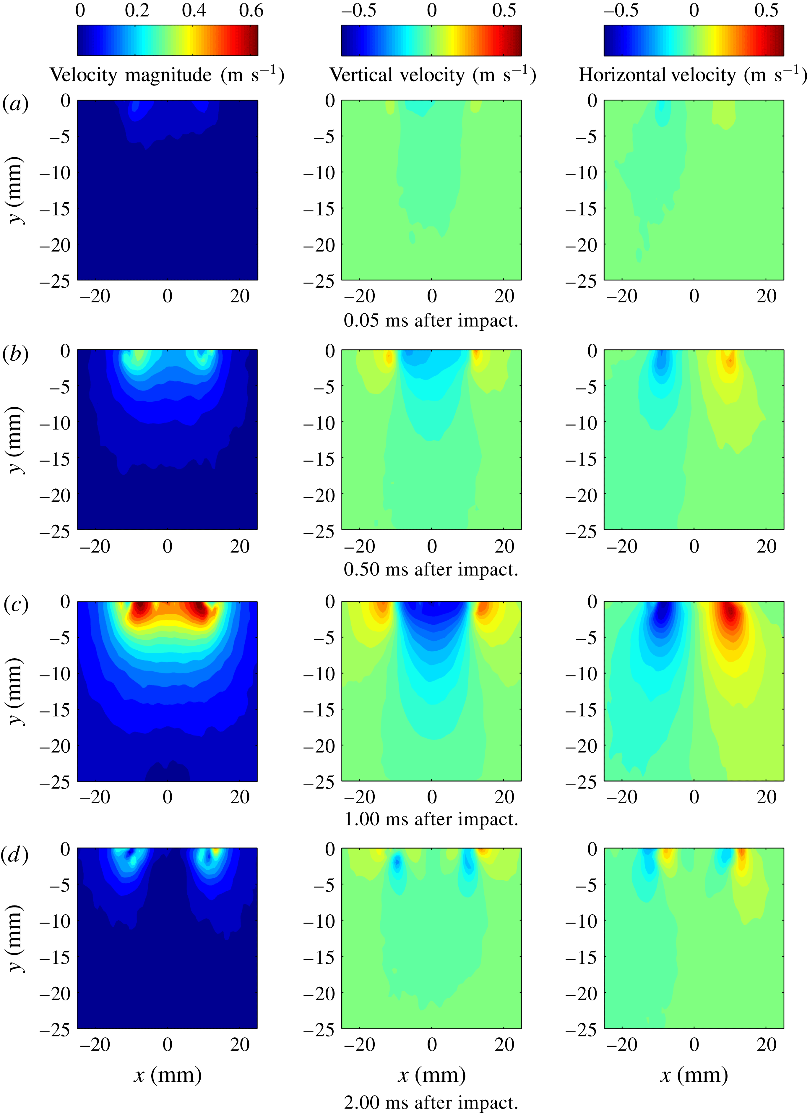
While PIV is commonly used to analyse steady flow fields, the water impact event is far from steady, taking place over of the order of several milliseconds. However, given the repeatability of the impact process – a characteristic that our experimental set-up possesses in the studied range of physical conditions (Appendix) – and capability to adjust the delay time of the first image (the first laser pulse), we were able to sweep through an entire impact event to build a time history, such as shown in figure 4.
PIV results showing the velocity magnitude and velocity components
 $v$
and
 $u$
(left to right), from individual water impact events for
 $w=10~\text{mm}$
,
 $V_{0}=0.5~\text{m}~\text{s}^{-1}$
and
 $h=1~\text{mm}$
.
The PIV velocity field measured
 $1~\text{ms}$
after the impact:
 $w=10~\text{mm}$
,
 $V_{0}=0.5~\text{m}~\text{s}^{-1}$
. The plate impacts water in this case. (a) Velocity magnitude
 $|\boldsymbol{v}|$
, (b)
 $v$
and (c)
 $u$
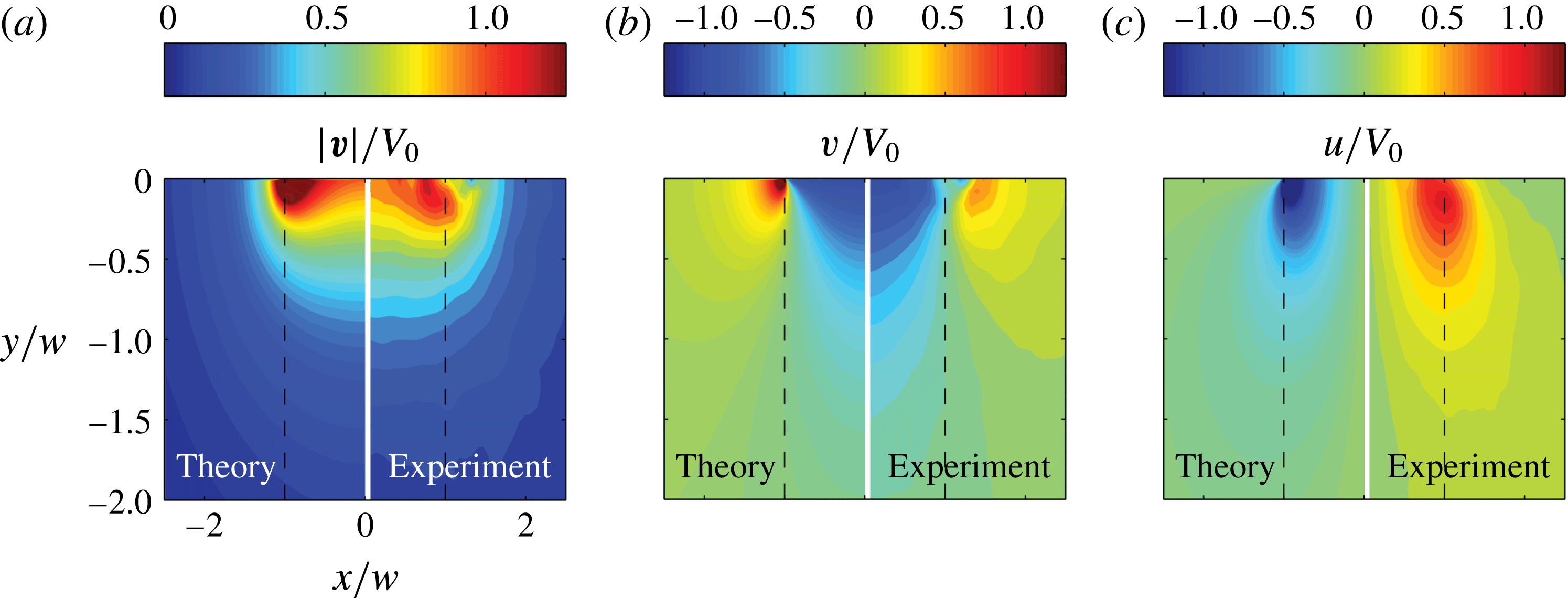
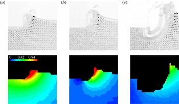
contour plots are shown side by side with the predictions from the inviscid theory (1.2).
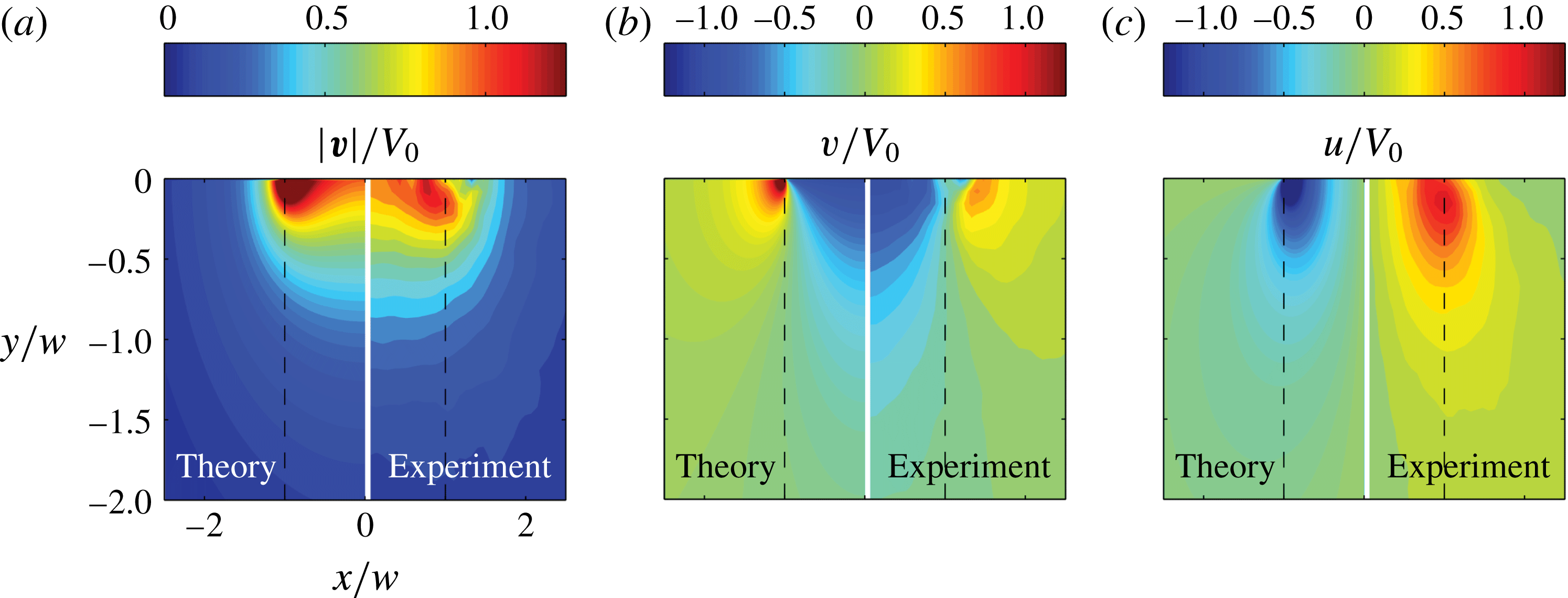
Figure 4 shows the basic stages of the impact process. In the moments shortly after the touchdown (a), the fluid possesses little (if any) velocity. After the impact (b), the flow field begins to take on the attributes described by the inviscid impact theory (1.2), see figure 1(b). Specifically, the velocity scalar magnitude is highest at the corners of the plate indicating that the liquid is driven toward the plate edges and then abruptly turned upward. If we look further in time, as in figure 4(c), the magnitudes of the velocity components increase as the plate penetrates into the liquid. As is obvious from (a) and (b), the flow does not develop instantly into the inviscid solution (1.2) as predicted by the ideal flow theory: since the event in (b) occurs considerably after the compressible effects propagate (
 $\unicode[STIX]{x0394}t_{c}=O(10^{-2})\,\text{ms}$
for the impact conditions in figure 4), such non-instant time development is caused by the trapped air which provides cushioning between the impactor and the liquid. Finally, when the plate has reached its limit of travel it is abruptly decelerated, along with most of the fluid, as seen in figure 4(d). But near the edge of the plate we can see the pocket of air – the horizontal velocity component reverses direction between (c) and (d). From further examination of figure 4 we can notice that during the initial stage (a), when the phenomena are most sensitive to any small misalignments and instabilities, the vertical velocity is symmetric, which means that the contact near both left and right plate edges is made simultaneously, while the horizontal velocity is not, which could be due to the asymmetry of the escaping trapped air layer caused by instabilities, e.g. of Kelvin–Helmholtz type. At later times the symmetry of the horizontal speed is recovered in (c), so that the flow field becomes symmetric. At the deceleration stage, because of its short time scale we are in the near-acoustic regime, see figure 3(b), which again becomes sensitive to any misalignments and instabilities, thus making the now-reversed flow field slightly asymmetric, see figure 4(d).
A direct comparison between the measured velocity field and that predicted by the inviscid theory (1.2) is provided in figure 5 and shows a remarkable similarity. This is perhaps not too surprising as the liquid was water for this set of measurements with
 $Re=5000$
. For a more quantitative comparison between liquids and better observation of any effect of viscosity let us consider the velocity profile
 $u(y)$
for a fixed time
 $t$
and value of
 $x$
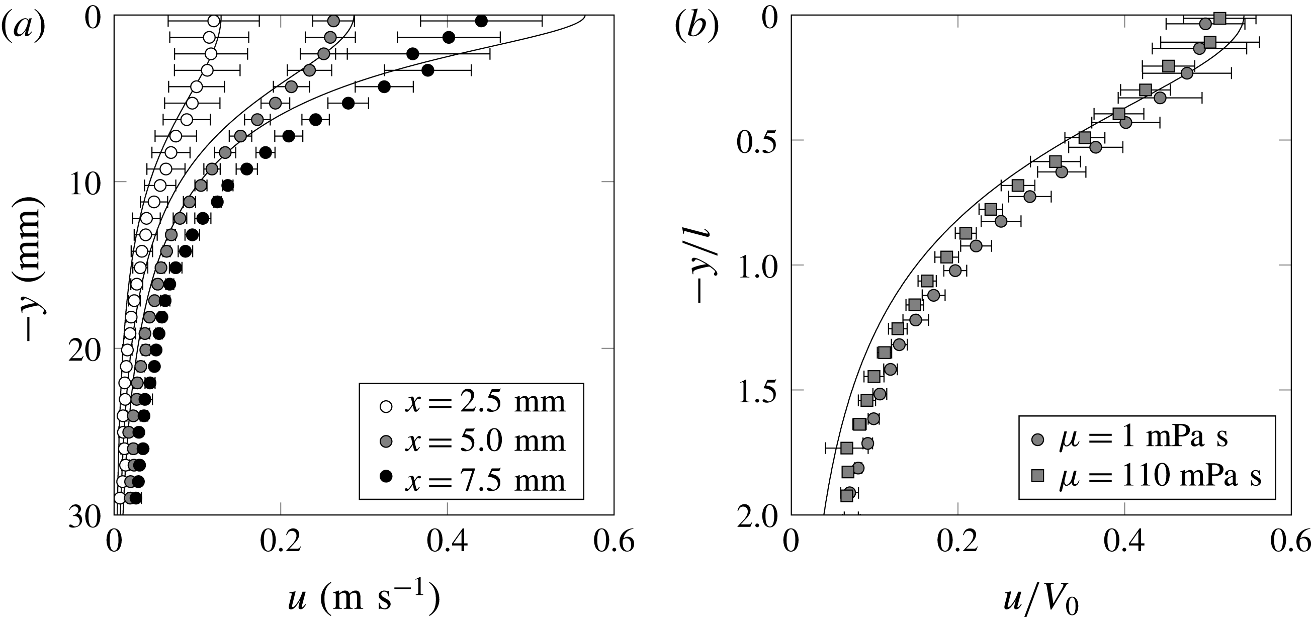
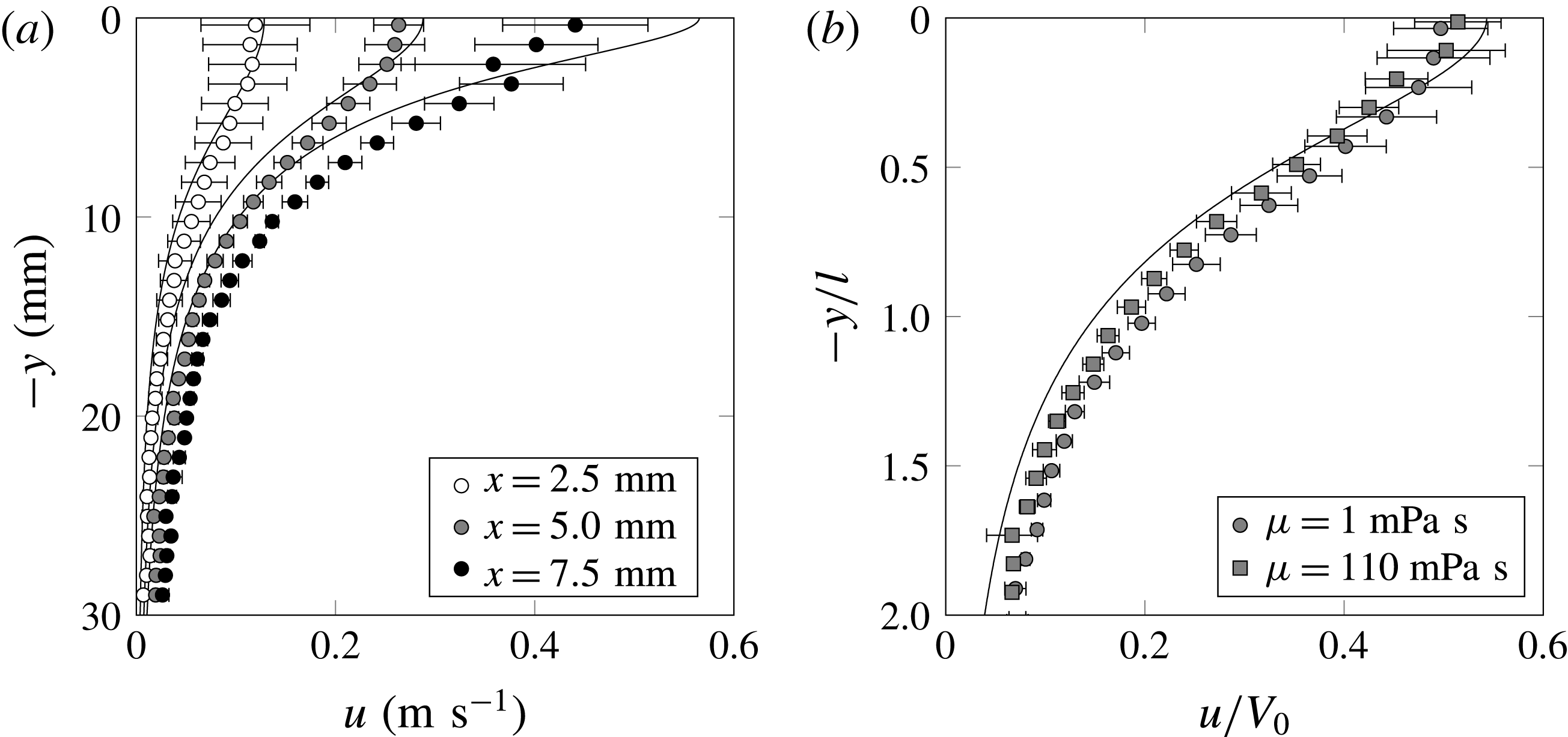
(refer to figure 1(b) for the coordinate system used). Figure 6(a) shows
 $u(y)$
for three values of
 $x$
for the case of water. There is reasonable agreement in the shape of the measured and theoretical profiles of
 $u(y)$
. However, we also observe that for small values of
 $y$
(close to the plate), the measured values of
 $u$
are less than predicted and for large values of
 $y$
they are greater than predicted. While the former discrepancy is likely due, in part, to the boundary layer that exists on the underside of the plate, the latter can be attributed, in part, to a non-negligible vertical penetration of the plate not accounted in the theory (1.2), which gives the ideal solution for
 $t\rightarrow +0$
only.
Velocity profile
 $u(y)$
for the plate
 $w=10~\text{mm}$
at
 $t=1~\text{ms}$
; here
 $x$
is the coordinate measured from the plate centre. (a) The
 $u(y)$
profiles for water only: there is reasonable agreement with the inviscid theory, based on the overlap of the data points and solid line (theory), for a range of
 $x$
extending to within a few millimetres of the plate edge. (b) This agreement persists for a factor of nearly 100 increase in liquid viscosity, but we find that
 $u(y)<u_{inv}$
near the plate and
 $u(y)>u_{inv}$
far from the plate. Profiles are shown at
 $x=5.0~\text{mm}$
only.
If we compare the results for two different liquids, with a factor of
 $O(10^{2})$
difference in viscosity, the agreement is also reasonable, as per figure 6(b). Here we plot
 $u(y)$
for
 $x/w=0.5$
, i.e. half-way between the plate centre and the edge. We notice that there does not appear to be a significant variation in
 $u(y)$
despite the large change in viscosity from
 $\text{Re}=50$
in the case of the glycerol solution to
 $\text{Re}=5000$
in the case of water used in figure 6(b), i.e. the Reynolds numbers are moderate to large in both cases. These measurements are well outside the boundary layer that grows on the underside of the plate as a consequence of the pressure-driven flow of liquid toward the edge and the no-slip condition imposed on the bottom surface of the plate. This boundary layer extends beneath and away from the plate to a depth
 $l_{\unicode[STIX]{x1D708}}=\sqrt{\unicode[STIX]{x1D708}\,t}$
: under the given experimental conditions this layer is
 $\mathit{O}(30~\unicode[STIX]{x03BC}\text{m})$
thick for water and
 $\mathit{O}(300~\unicode[STIX]{x03BC}\text{m})$
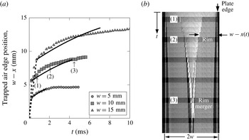
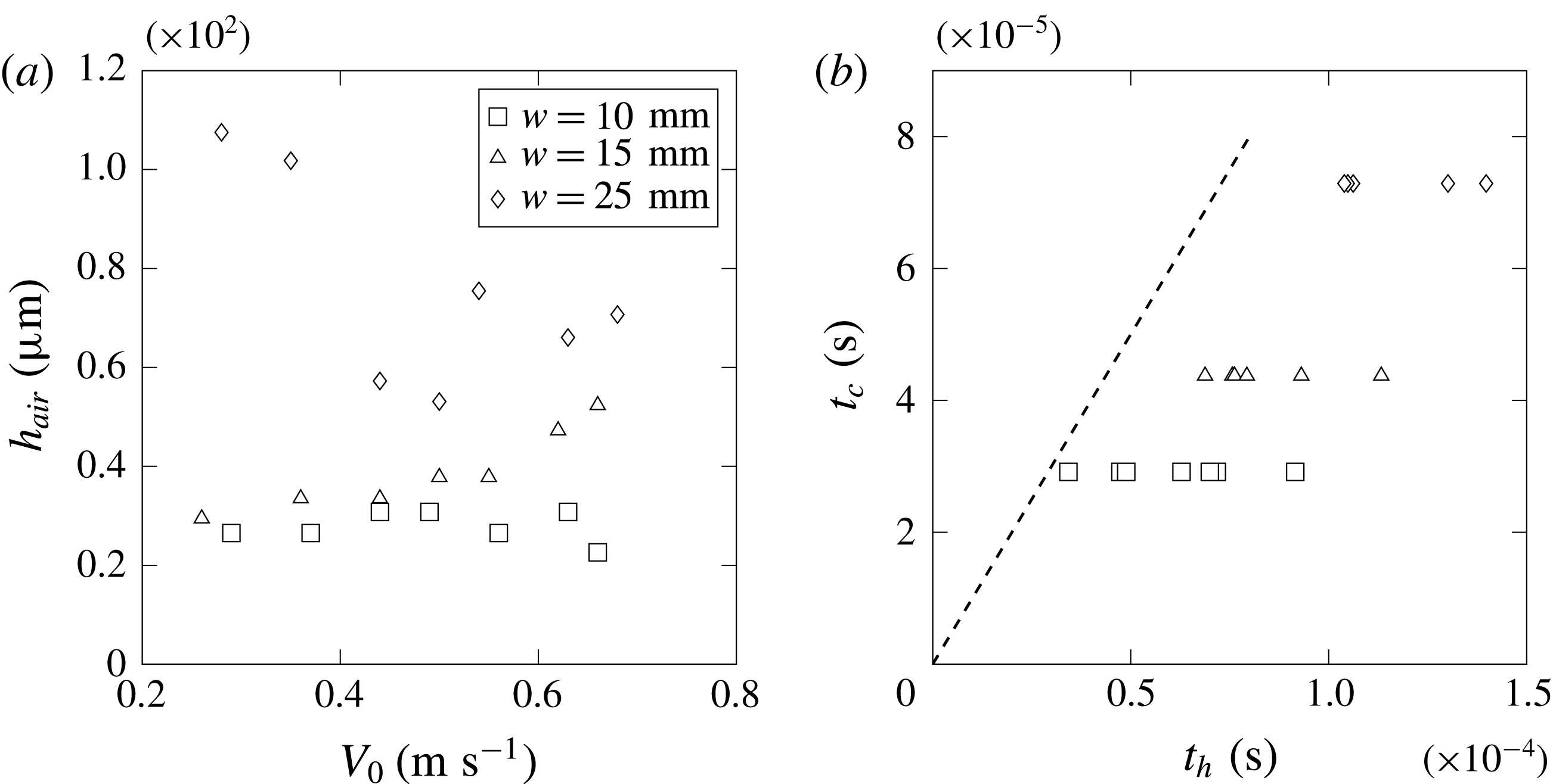
for the water–glycerin solution used in figure 6(b). These values are below the resolution of the system at this magnification. The boundary layer picture is further complicated by the thin layer of trapped air that prevents immediate contact of the liquid with the plate surface (§ 5).
3.3 Local velocity field
In an effort to investigate the flow field near the edge, we performed a set of tests using higher magnification lenses on the PIV camera as well as changing the plate width
 $w$
and impact speed
 $V_{0}$
. Given that the characteristic time is defined as
 $\unicode[STIX]{x1D70F}=w/V_{0}$
, in order to experimentally achieve the conditions
 $\widetilde{t}=t/\unicode[STIX]{x1D70F}\ll 1$
and
 $r/w\ll 1$
, we can decrease the impact velocity and/or increase the plate width. Challenges exist with both approaches. Decreasing
 $V_{0}$
reduces the magnitude of the velocity field after impact. Hence, increased laser pulse delays are needed to obtain accurate velocity information using PIV. For a shorter duration impact event (due to the decreased
 $V_{0}$
), this translates into fewer snapshots that can be captured to form a sequence. On the other hand, increasing
 $w$
provides more information closer to the edge (i.e. smaller
 $r/w$
regions can be accessed optically), but also increases the impact
 $We$
, which in turn creates a narrower, more vertically directed ejecta as it is equivalent to increasing the impact velocity
 $V_{0}$
. This makes gathering velocity field information near the inner ejecta profile difficult as well. In what follows, results for variations in both experimental conditions – impact velocity and plate width – will be presented for water as the impacted liquid.
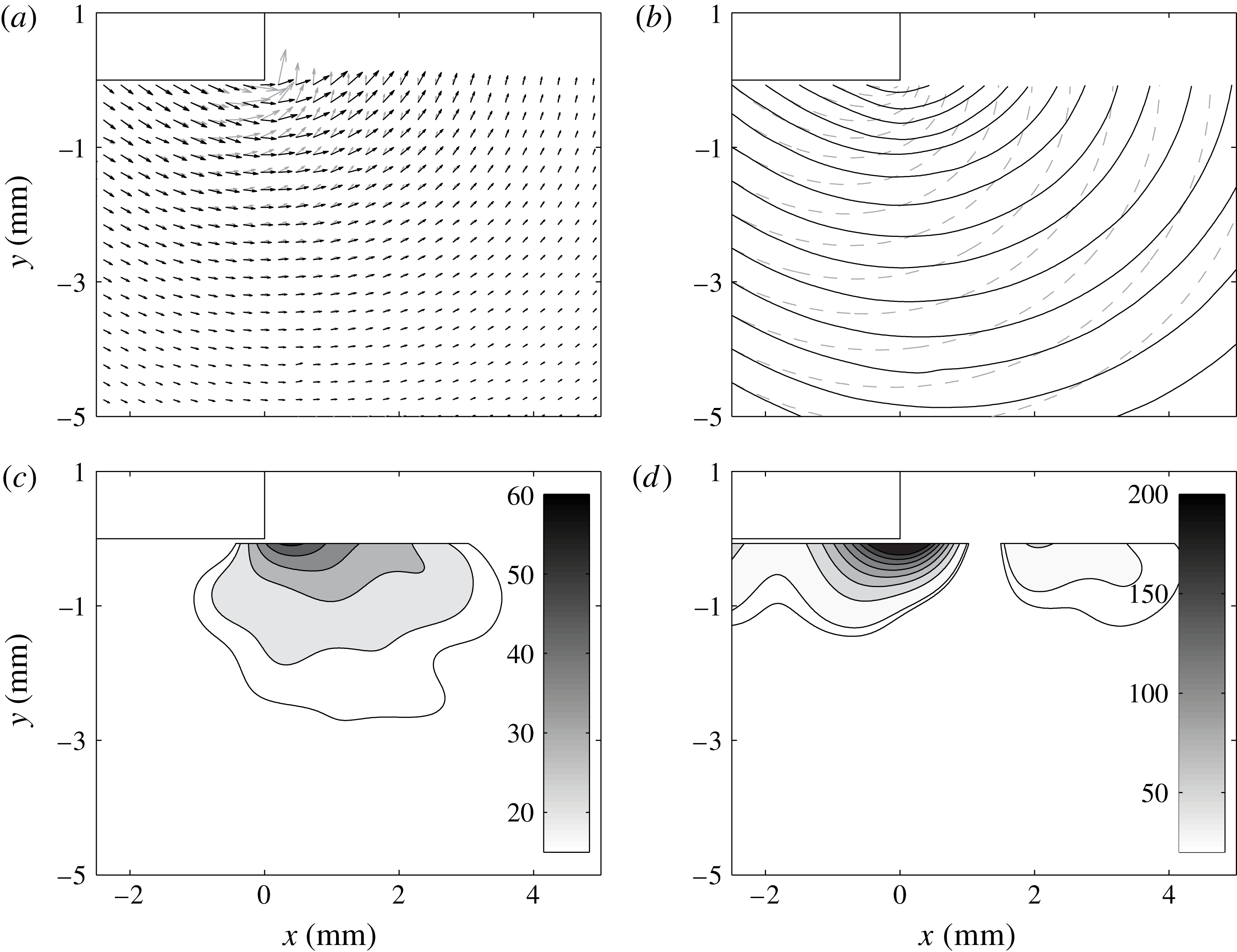
A direct comparison of the velocity vector angle and magnitude, and streamlines trajectory between the inviscid theory (1.2) (grey, dashed) and PIV measurements (black, solid). Considerable disagreement exists near the edge where the liquid must negotiate the turn at the corner without a singularity – hence the more shallow (i.e. smaller angle measured with respect to the free surface) velocity vectors (a) and streamlines (b) compared to the theory. The difference in angle (measured in degrees) between theory and experiment is shown in the contour plot of (c). The per cent difference (d) between the magnitude of the theoretical and experimental velocity vectors shows that significant disagreement is contained in a region near the plate edge. Experimental conditions correspond to water impact with a plate of dimension
 $w=10~\text{mm}$
and impact velocity of
 $V_{0}=0.18~\text{m}~\text{s}^{-1}$
resulting in
 $We=5$
. The velocity field corresponds to
 $2~\text{ms}$
after impact (dimensionless time of
 $\widetilde{t}=0.04$
, where
 $\widetilde{t}=t/\unicode[STIX]{x1D70F}$
).
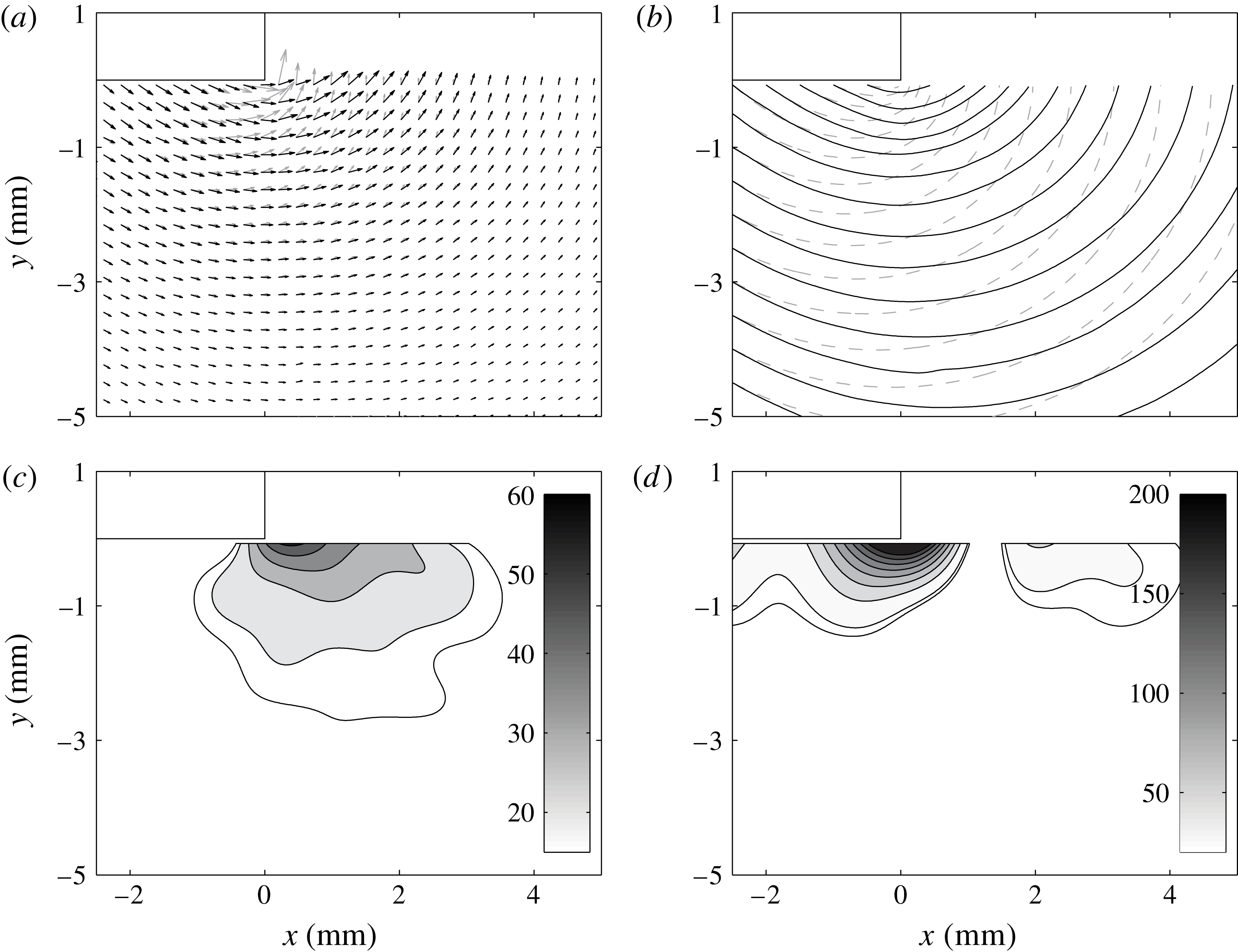
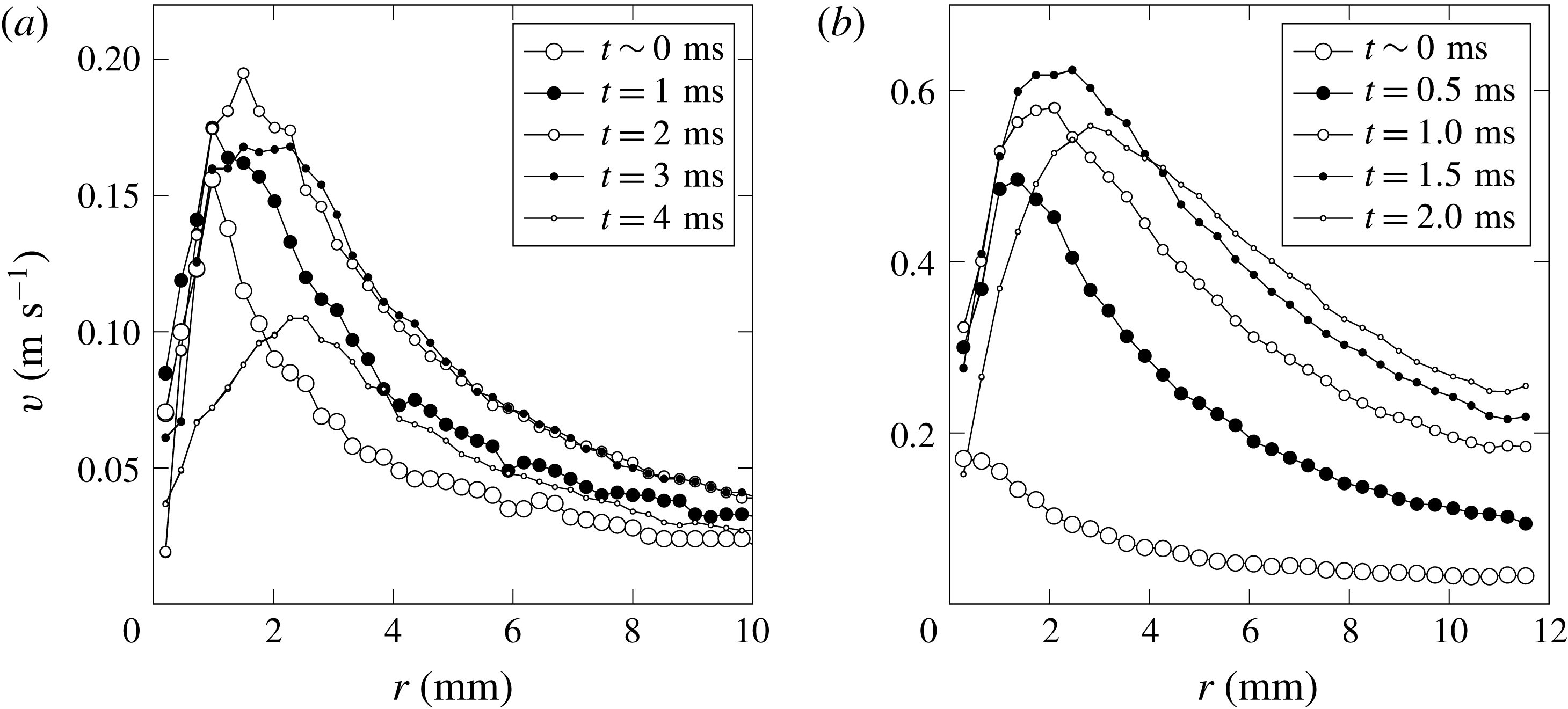
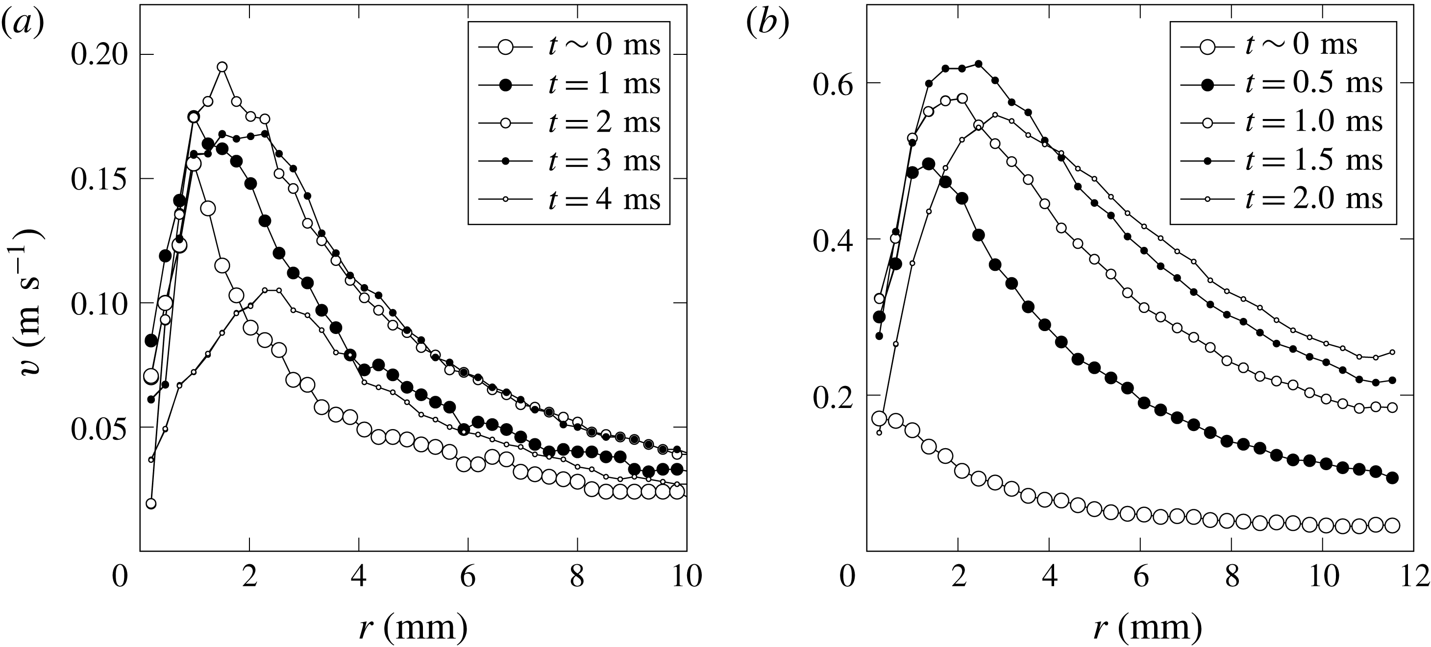
A basic illustrative example of the quantitative near-edge velocity field is provided in figure 7, which allows us to test the existing theory for the scaling of the velocity field in space and time below. Figure 8 shows for two plate sizes the variation of the vertical component of the liquid velocity with position from the edge and time after the impact, at a depth corresponding to the level of the impact plate bottom,
 $\unicode[STIX]{x1D703}=0^{\circ }$
. At any given time, the velocity first increases and then decreases as
 $r$
increases. This is consistent with the observed ejecta development.
Dimensional plots of the vertical velocity component
 $v$
as a function of
 $r$
for
 $\unicode[STIX]{x1D703}=0^{\circ }$
(i.e. near the pre-impact free surface, and at the depth of the bottom of the plate) for five values of
 $t$
after impact: (a)
 $w=10~\text{mm}$
and
 $V_{0}=0.18~\text{m}~\text{s}^{-1}$
, (b)
 $w=25~\text{mm}$
and
 $V_{0}=0.54~\text{m}~\text{s}^{-1}$
. The start of the abrupt decelerations of the plates is captured in the last profile of each sequence exhibiting a dramatic reduction in the velocities. For the narrower plate (a), the dimensional range of time is
 $0\leqslant t<4~\text{ms}$
, whereas for the wider plate (b), it is
 $0\leqslant t<2~\text{ms}$
. The dimensional times for (a) correspond to
 $\widetilde{t}=t/\unicode[STIX]{x1D70F}$
of 0.000, 0.018, 0.036, 0.054, 0.072, and for (b) 0.000, 0.011, 0.022, 0.032 and 0.043. The range of dimensionless times corresponding to the impact event for the larger plate is shorter than that for the smaller plate.
As the velocity field near the edge is predicted by (1.2) to scale with
 $r$
as
 $\boldsymbol{v}\sim r^{-1/2}$
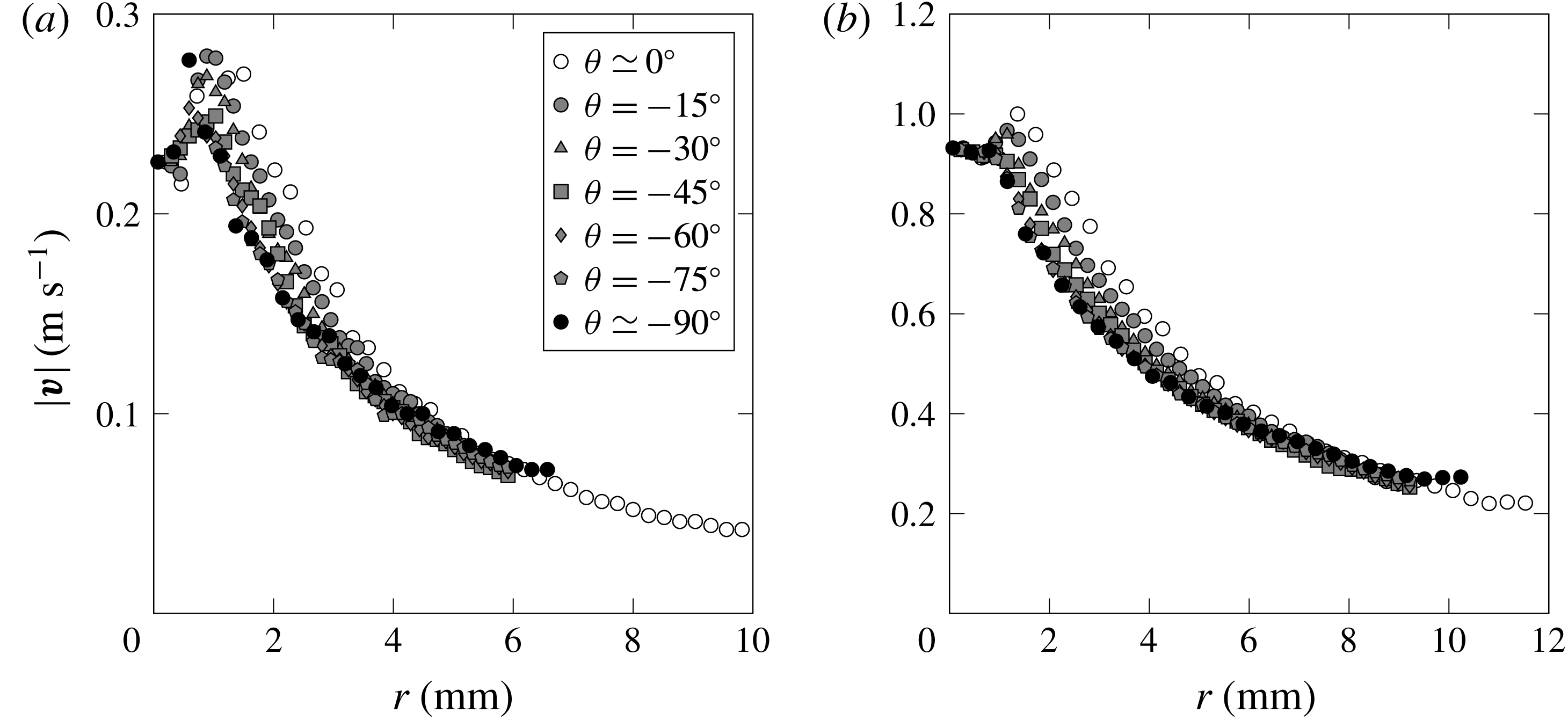
, it is necessary for comparison to extract the velocity magnitude along rays (in the
 $r$
direction) at constant values of
 $\unicode[STIX]{x1D703}$
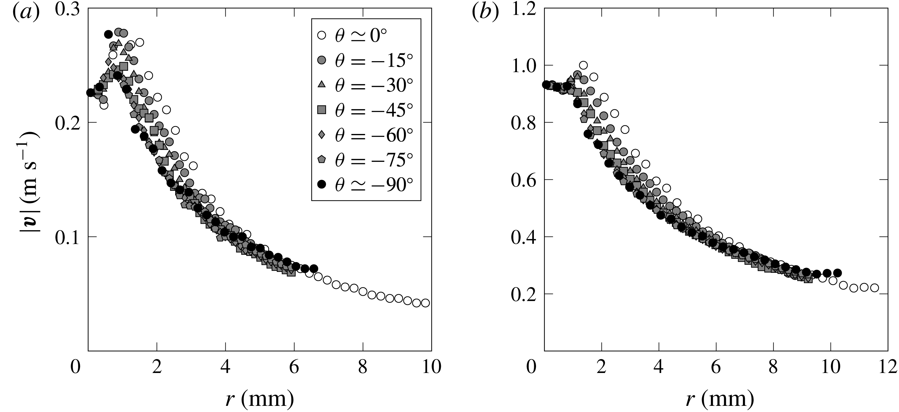
from the PIV measurements, as illustrated in figure 9. Here we see that the magnitude of velocity near the edge of the plate is nearly independent of ray angle as anticipated by the inviscid solution (1.3). In an effort to quantify and display the relationship between
 $|\boldsymbol{v}|$
and
 $r$
, we have chosen to provide a series of plots for
 $|\boldsymbol{v}|$
versus
 $r$
, for the two impact plates sizes and velocities.
Variation in velocity magnitude
 $|\boldsymbol{v}|$
in the radial direction from the plate corner for various values of the angle
 $\unicode[STIX]{x1D703}$
in the impact on water: (a)
 $\widetilde{t}=0.054$
;
 $w=10~\text{mm}$
,
 $V_{0}=0.18~\text{m}~\text{s}^{-1}$
,
 $We=5$
, (b)
 $\widetilde{t}=0.032$
;
 $w=25~\text{mm}$
,
 $V_{0}=0.54~\text{m}~\text{s}^{-1}$
,
 $We=90$
. The velocity profiles are essentially independent of angle
 $\unicode[STIX]{x1D703}$
. Near the plate,
 $r<1~\text{mm}$
, the velocity increases with
 $r$
.
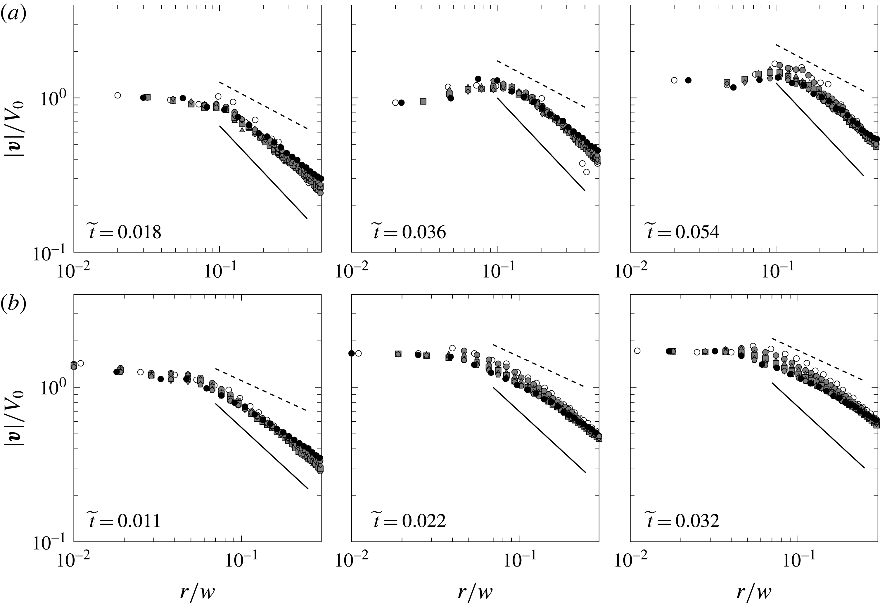
Detailed view of the velocity data in log axes: dimensionless velocity in the normalized radial direction for
 $We=5$
and
 $Re=1800$
corresponding to
 $w=10~\text{mm}$
and
 $V_{0}=0.18~\text{m}~\text{s}^{-1}$
(a);
 $We=90$
and
 $Re=5400$
corresponding to
 $w=25~\text{mm}$
and
 $V_{0}=0.5~\text{m}~\text{s}^{-1}$
(b). Only the portion of the flow field for which
 $r/w<0.35$
is shown. The solid and dashed lines have slopes of
 $-1$
and
 $-1/2$
, respectively, and are added for comparison. Marker symbols are the same as in figure 9.

With the goal of comparing the velocity scaling with the short distance from the edge
 $r\rightarrow 0$
to the inviscid theory, we restrict the field of view to
 $r/w<0.35$
for the log–log plots in figure 10 so that the exponent associated with the decrease in velocity with
 $r$
can be observed more clearly. The solid lines and dashed lines correspond to a slope of
 $-1$
and
 $-1/2$
, respectively, and are provided for comparison to the data. The top row of plots presents PIV data for the impact experiments corresponding to
 $We=5$
, while the bottom row to
 $We=90$
. From left to right the plots are in increasing order of dimensionless time
 $\widetilde{t}=t/\unicode[STIX]{x1D70F}$
. We can see that at the later times closest to the plate there is a region of increasing velocity. This is most apparent in the low
 $We$
plots. Following this is a region of decreasing velocity as we move away from the plate edge: the velocity profiles converge for large
 $r/w$
since the influence of viscosity and surface tension is weakened at such distances. However, for the same reason the growth of
 $\boldsymbol{v}$
is slowed down and one observes a substantial scatter near the plate edge,
 $r/w\rightarrow 0$
, where the effects of viscosity and surface tension are pronounced. Also, the bottom row exhibits a thinner boundary layer near the plate because of the higher Reynolds number. From figure 10 it transpires that
 $\boldsymbol{v}\sim r^{-1/2}$
corresponding to the inviscid theory is observed only transiently for a very narrow range of distances.
We first recognize that the actual velocity field may deviate from the inviscid theory owing to the existence of a trapped air layer beneath the impact plate. Yet, the effect of this air layer is not readily quantifiable, as we do not know the exact shape of the layer at impact or during penetration, and how this may influence the fluid flow around the corner of the plate. Second, while we are considering the results from experiments for the reduced
 $r/w$
scale made as small as possible, ideally probing
 $r/w\ll 1$
to compare with theory, in reality we are limited to investigating a region
 $r/w<1$
with the smallest range for PIV measurements of the order of
 $r/w\sim 10^{-2}$
. So the natural question is how applicable are the theoretical predictions of equation (1.3) to the data we obtain? To address this question, let us consider a comparison between the velocity profile
 $v(x,y=0)$
for the two impact
 $We$
cases and the two forms of the inviscid flow theory – the full solution (1.2) valid for all
 $r$
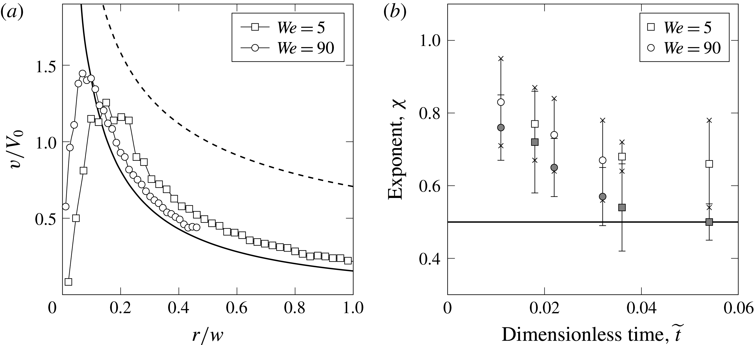
and the near-edge result (1.3) in figure 11(a). From this figure we can observe that the data in the range of
 $r/w>0.1$
appear to match the full inviscid flow theory (1.2) reasonably well, both in magnitude and in dependence on
 $r$
. Other than that, there is poor agreement between the data and the near-edge asymptotics (1.3): certainly, the power law near the edge
 $\boldsymbol{v}\sim r^{-1/2}$
is not observed, which is expected from deviations in figure 7, since real physical effects near the plate edge – air entrapment, viscosity, wetting and surface tension – modify the flow field at the leading order due to the singular perturbation nature of the problem (cf. § 1.2).
(a) A comparison of the inviscid velocity profiles
 $v(r,\unicode[STIX]{x1D703}=0^{\circ })$
against PIV measurements for
 $We=5$
and
 $We=90$
. The solid line is from the full inviscid flow solution (1.2) and the dashed line is from asymptotics (1.3). We can immediately recognize that there is reasonable agreement between the full solution and the data, with the exception of
 $r/w<0.1$
. (b) The exponent
 $\unicode[STIX]{x1D712}$
associated with the decay in velocity magnitude along the radial location for various values of
 $\unicode[STIX]{x1D703}$
and for several instants in time
 $\widetilde{t}$
. We have used the velocity field information from PIV measurements to find
 $\boldsymbol{v}(r)$
. Beyond the peak in velocity magnitude, the values appear to decrease as
 $r^{-\unicode[STIX]{x1D712}}$
, where
 $r^{-1/2}$
is predicted by inviscid theory. Open symbols are based on
 $0.07<r/w<0.35$
(wide plate) and
 $0.1<r/w<0.35$
(narrow plate). Grey-filled symbols use a reduced range with an upper limit of
 $r/w=0.2$
.

Quantitative analysis of the slopes of the velocity profiles in figure 10 is shown in figure 11(b) as the
 $r^{-\unicode[STIX]{x1D712}}$
velocity dependence. The marker value
 $\unicode[STIX]{x1D712}$
for each time
 $\widetilde{t}$
is the average exponent for all curves of constant
 $\unicode[STIX]{x1D703}$
near the edges so as to correspond to
 $r\rightarrow 0$
. The error bars for the data points in figure 11(b) illustrate the range of values for each
 $\widetilde{t}$
. In general, the exponents all fall above
 $-1/2$
and below
 $-1$
, with the former being the prediction from the inviscid flow theory near the edge. Note, however, that by using only smaller values of
 $r/w$
the values of the exponents
 $\unicode[STIX]{x1D712}$
will decrease as the slope of the profiles tends to become shallower. For example, compare the grey-filled and open symbols in figure 11(b), where the former are obtained by extracting the slopes for the data with a reduced range in which the upper limit of
 $r/w$
set as
 $0.2$
instead of
 $0.35$
. Values from measurements presented in figure 11(b) suggest that
 $\unicode[STIX]{x1D712}\sim 0.6{-}0.8$
. Although the full inviscid solution (1.2) does not have power-law behaviour (note the change in slope in figure 11
a) if we were to fit a power-law trend to the portion of the curve between
 $0.05<r/w<0.35$
we would find that it behaves as
 $r^{-0.80}$
. As follows from figure 11(a), the region where
 $\boldsymbol{v}\sim r^{-1/2}$
would be observable,
 $r/w\ll 1$
, simply does not exist as the velocity profile falls due to physical effects as opposed to continue growing with
 $r\rightarrow 0$
according to (1.3).
3.4 The Kutta–Joukowsky condition
An important insight can be gained by measuring the angle at which the fluid interface departs from the plate edge shown in figure 12. As we can see from figure 12(a), the initial departure is very far from being horizontal and thus from being consistent with the KJ condition, but for later times it attenuates to nearly perfect wetting (
 $\unicode[STIX]{x1D717}=0$
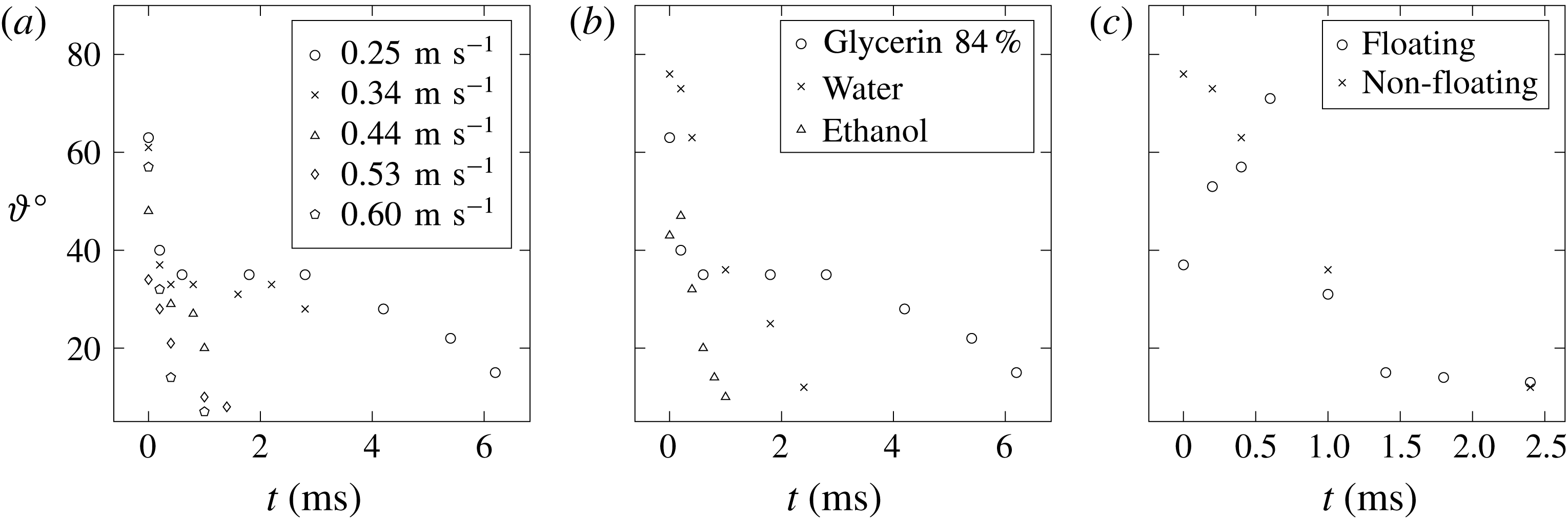
) at a rate increasing with the impact speed. The initial direction of the departing velocity vectors in figure 12(b) is correlated with the wettability of the liquid with respect to the solid (stainless steel): the apparent static contact angle
 $\unicode[STIX]{x1D717}$
ranges from
 $72^{\circ }$
for water down to
 $27^{\circ }$
for high concentration glycerin consistent with the data reported by Moldovan et al. (Reference Moldovan, Bota, Boerasu, Dorobantu, Bojin, Buzatu and Enachescu2013), and to
 $15^{\circ }$
for ethanol, i.e. static wetting is never perfect for our choice of liquids. Figure 12(b), comparing the dynamics for three different liquids, suggests that wettability may affect the departure angle in a dynamic way, though non-monotonicity of the behaviour at later times (water wets less than glycerin, which in turn wets less than ethanol) points out that differences in viscosity and surface tension may have a significant dynamic effect as well. Figure 12(c) shows the difference in the departure angle evolution between impacts of a floating and non-floating plates, which indicates how the edge condition affects the splashing. While the non-floating case studied in this paper follows the behaviour in figure 12(a), the floating plate with razor-sharp edge aligned with the initially undisturbed water surface has a much smaller (though non-negligible) departure angle of the static interface (when the plate is not moving), but after the impact the angle increases, approaching that of the non-floating case, and then attenuates with time as in the latter case. Such a noticeable difference in the initial evolution of the contact angle (and hence ejecta) is consonant with the earlier observations of Yakimov (Reference Yakimov1973) and Ermanyuk & Ohkusu (Reference Ermanyuk and Ohkusu2005), who found that the presence of a trapped air is analogous to the effect of hydrophobicity and significantly affects the ejecta development. Another example of how wetting properties alter the splashing is given by Duez et al. (Reference Duez, Ybert, Clanet and Bocquet2007) in the context of water impact by spheres penetrating at substantial depth.
On the angle
 $\unicode[STIX]{x1D717}$
at which the fluid interface departs the plate. (a) Variation of
 $\unicode[STIX]{x1D717}$
with time and impact velocity
 $V_{0}$
for the
 $100~\text{mPa}~\text{s}$
water–glycerol solution. (b) Difference in the departure angle evolution between impacts on glycerin, water and ethanol. (c) Difference in the departure angle evolution between impacts of a floating and non-floating flat plates on water.

Given the above observations, several comments are in order. In the inviscid approximation studies, e.g. by Zhao, Faltinsen & Aarnes (Reference Zhao, Faltinsen, Aarnes and Rood1996) and Iafrati & Korobkin (Reference Iafrati and Korobkin2004, Reference Iafrati and Korobkin2008, Reference Iafrati and Korobkin2011), an additional constraint – the KJ-type condition – was enforced at the plate edge requiring that the free surface leaves the plate edge tangentially for
 $t\geqslant 0$
, which in turn implies that the flow does not make a sharp right angle turn upon leaving the plate edge, in contrast to the inviscid complex variable solution (1.2). However, having ascertained that the solution of (1.1) is unique, we conclude that, as opposed to the mechanism for imposing the KJ condition in the airfoil theory – variation of circulation around airfoil (which makes the effect of the KJ condition global) – introduction of such an extra condition would either overdetermine the system or change the boundary condition (1.1b
), so that it would be a physically different problem. Thereby, the resolution of the edge singularity in the water impact problem lies outside the realm of the inviscid formulation (Krechetnikov Reference Krechetnikov2018), which can be appreciated from the following considerations.
First, recall that in the problems of vortex shedding (such as in the airfoil theory or when an object with sharp edges moves through a fluid), the KJ condition in the potential inviscid approximation – streamline leaving the trailing edge tangentially – is imposed to prevent the velocity at the trailing edge from becoming infinite. The KJ condition in such problems is viable as allowed by non-uniqueness of the solution of the corresponding boundary-value problem and physically enabled by viscosity leading to the boundary layer separation. From Bernoulli’s equation (or, in the unsteady cases, the Cauchy–Lagrange integral) in the bulk, this implies that the pressure must be bounded as well. When
 $t>0$
, in the problem of a plate suddenly moving in its normal direction, the vortex will be shed from the edge, which leaves the plate tangentially (Jones Reference Jones2003; Semenov & Wu Reference Semenov and Wu2018) provided the KJ condition is satisfied. In the water entry problem, on the other hand, it is directly assumed (e.g. Iafrati & Korobkin (Reference Iafrati and Korobkin2004)) that the flow direction is tangential to the body surface at the plate, and is a result of ensuring finite velocity at this point, but not finite pressure. Indeed, in the water impact problem, despite the fact that the velocity at
 $t=0+$
is infinite near the plate edge, the pressure is still continuous in space and approaches that of the atmosphere as can be seen from the impulsive pressure on the bottom of the plate
 $\int p~\text{d}t\sim \sqrt{w^{2}-x^{2}}\rightarrow 0$
near the plate edges
 $x\rightarrow \pm w$
.
However, requiring boundedness of the velocity in the inviscid potential formulation is not always possible as it depends on the nature of the problem at hand. Even in the airfoil theory, when the airfoil is a flat plate with both leading and trailing edges being sharp, the KJ condition removes the singularity at the trailing edge only, while at the leading edge the velocity is still singular. Another classical example is the incompressible flow outside an angle
 $\unicode[STIX]{x1D703}>\unicode[STIX]{x03C0}$
formed by two intersecting planes (Landau & Lifshitz Reference Landau and Lifshitz1987) with the singularity being
 $\boldsymbol{v}\sim r^{n-1}$
,
 $n=\unicode[STIX]{x03C0}/\unicode[STIX]{x1D703}$
. The water impact problem belongs to the latter class of problems and, in fact, the velocity unboundedness
 $\boldsymbol{v}\sim r^{-1/2}$
follows exactly from the problem of the flow outside an angle of
 $2\unicode[STIX]{x03C0}$
(i.e. around the plate edge). The same behaviour is also observed in the teapot phenomenon (Keller Reference Keller1957): as the liquid flows around a spout lip, its velocity is the greatest at the lip, which means that the pressure inside the liquid stream is then the lowest and hence the surrounding air at atmospheric (and thus higher) pressure will push the liquid against the lip. Effectively, the liquid is capable of making a sharp turn. Also, in the problem of gliding on water, where there are two jets leaving from the leading and trailing edge (Sedov Reference Sedov1965), under certain conditions the spray jet leaves the leading edge not necessarily tangentially (Green Reference Green1936).
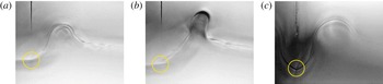
The free surface does not necessarily leave the plate edge (still during the penetration stage) tangentially as assumed in the KJ condition – the point where the free surface leaves the impactor is encircled. Wide plate of
 $w=25~\text{mm}$
was used. Impact conditions: (a) water,
 $t=2.4~\text{ms}$
,
 $V_{0}=0.14~\text{m}~\text{s}^{-1}$
; (b) water,
 $t=2.2~\text{ms}$
,
 $V_{0}=0.28~\text{m}~\text{s}^{-1}$
; (c) water–glycerol solution with
 $\unicode[STIX]{x1D707}=100~\text{mPa}~\text{s}$
,
 $t=4.6~\text{ms}$
,
 $V_{0}=0.28~\text{m}~\text{s}^{-1}$
. Capillary waves distinctly seen in (a) destroy self-similarity. The spatial resolution is higher than
 $O(10^{-2})~\text{mm}$
, which is considerably below the viscous length scale
 $l_{\unicode[STIX]{x1D708}}=O(10^{-1})~\text{mm}$
in (a,b) and
 $l_{\unicode[STIX]{x1D708}}=O(10^{0})~\text{mm}$
in (c).

In our context, the KJ condition is used (and needed) only in the approximation, which neglects viscosity and surface tension – therefore, the (expected zero) departing angle should be measured at the distances from the edge where such an inviscid approximation is valid. Both viscosity and surface tension introduce corresponding length scales
 $l_{\unicode[STIX]{x1D708}}$
and
 $l_{\unicode[STIX]{x1D70E}}$
to be determined below and in § 4.2, respectively, so the classical inviscid theory should be applicable at the distances larger than
 $\max \{l_{\unicode[STIX]{x1D708}},l_{\unicode[STIX]{x1D70E}}\}$
. Viscosity exhibits itself in a boundary layer (wall jet) growing as
 $l_{\unicode[STIX]{x1D708}}=\sqrt{\unicode[STIX]{x1D708}\,t}$
, which comes from its diffusive character. There is no fundamental principle which requires viscous flows to leave the edge tangentially, which are known to be able to make sharp turns (Moffatt Reference Moffatt1964). In particular, the slow Stokes flow in the immediate neighbourhood of the plate edge,
 $r\rightarrow 0$
, permits the interface to assume the non-zero departing angle dictated by wetting properties between liquid, air and the plate; then viscosity smooths out the corner flow so that the outer inviscid flow follows an effectively smooth surface making a turn dictated by the wetting properties – there is no infinite velocity in this case, so that the inviscid flow is regularized. Apparently, this is different from simply enforcing the tangential departure (the KJ condition), since the latter does not encode the information about a non-zero departing angle
 $\unicode[STIX]{x1D717}$
the ejecta should follow.
The resolution of at least
 $10^{-2}~\text{mm}$
of our imaging is well below
 $\max \{l_{\unicode[STIX]{x1D708}},l_{\unicode[STIX]{x1D70E}}\}$
, so that we can resolve the transition between the inner (viscous) solution and the outer (inviscid) region and thus indeed assert that the departing angle is non-zero for the purpose of the inviscid theory (figure 13). As follows from the discussion in § 4.2, both
 $l_{\unicode[STIX]{x1D708}},l_{\unicode[STIX]{x1D70E}}\rightarrow 0$
as
 $t\rightarrow 0$
. Compared to the incompressible inviscid potential theory in which the flow is set instantaneously for
 $t=0^{+}$
due to infinite sound speed, in real experiments nothing has moved for
 $t=0^{+}$
in view of finite speed of sound, etc. In fact, because of the cushioning effect of trapped air, the pressure impulse lasts a finite time
 $O(w/c_{air})$
, cf. Chuang (Reference Chuang1966), that is longer than acoustic time in the impacted liquid
 $w/c_{0}$
. Hence, the idealized solution (1.2) at
 $t=0^{+}$
is observable only as a global approximation (i.e. not valid locally near the plate edges) over some short range of intermediate times after the acoustic stage (figure 4). Since in the real experiment at
 $t=+0$
no fluid has turned yet, no hypothetical vortex shedding could take place as needed to justify the KJ condition in the initially vortex-free flow. We generally do not observe tangential departure for positive times as well thus invalidating application of the KJ condition in the regime of finite
 $Re$
and
 $We$
number flows explored here. The overall conclusion is that the near-edge singularity of the solution (1.2) is resolved by viscosity and surface tension as opposed to by a KJ condition; in other words, these physical effects do not enable the KJ condition in contrast to, for example, the flow around an airfoil or around a plate moving in the fluid (Jones Reference Jones2003), in which viscosity is responsible for the tangential boundary layer separation. Having said that, applying the KJ condition in numerical experiments for large scale applications
 $w\gg \max \{l_{\unicode[STIX]{x1D708}},l_{\unicode[STIX]{x1D70E}}\}$
should have little quantitative effect on loads and other global characteristics, which is physically because the kinetic energy and impulse of the singular near-edge region are negligible due to its infinitesimally small mass despite the divergent velocity field (1.3). This can also be demonstrated mathematically using the global measure (e.g.
 $L^{2}$
-norm) of the solution of (1.1), which after integration by parts produces the direct link to the boundary data
 $\Vert \boldsymbol{v}\Vert ^{2}=\int _{\mathbb{H}^{-}}|\unicode[STIX]{x1D735}\unicode[STIX]{x1D719}|^{2}~\text{d}\boldsymbol{x}=\unicode[STIX]{x1D719}\,\unicode[STIX]{x1D735}\unicode[STIX]{x1D719}|_{y=0}$
, where we took into account (1.1a
). Hence, any local near-edge non-singular perturbation of the boundary condition (1.1b
) will not change
 $\Vert \boldsymbol{v}\Vert ^{2}$
appreciably. However, as suggested by our observations, the condition at the plate edge should have a significant effect on the local velocity field and ejecta evolution, especially if one were to compare an inviscid solution to the finite
 $Re$
and
 $We$
numbers data (Iafrati & Korobkin Reference Iafrati and Korobkin2004).
3.5 Test of Yakimov’s scaling
Having the time-sequenced PIV information at our disposal, we can also test the validity of Yakimov’s scaling based on the measured velocity field near the plate edge. To do this, we use the magnitude of the velocity field close to the edge, i.e.
 $r/w<1$
, along the radial direction for three angles:
 $\unicode[STIX]{x1D703}=0^{\circ },-45^{\circ },-90^{\circ }$
. The magnitudes of the velocity field and the radial dimension are scaled as follows. If the velocity field varies as
 $|\boldsymbol{v}|/V_{0}\sim r^{-\unicode[STIX]{x1D712}}$
, then based on Yakimov’s argument, i.e. that
 $\boldsymbol{v}\sim \text{d}\boldsymbol{r}/\text{d}t\sim r^{-\unicode[STIX]{x1D712}}$
, we should plot the scaled fields as
 $(|\boldsymbol{v}|/V_{0})\,t^{\unicode[STIX]{x1D712}/(1+\unicode[STIX]{x1D712})}$
versus
 $(r/w)\,t^{-1/(1+\unicode[STIX]{x1D712})}$
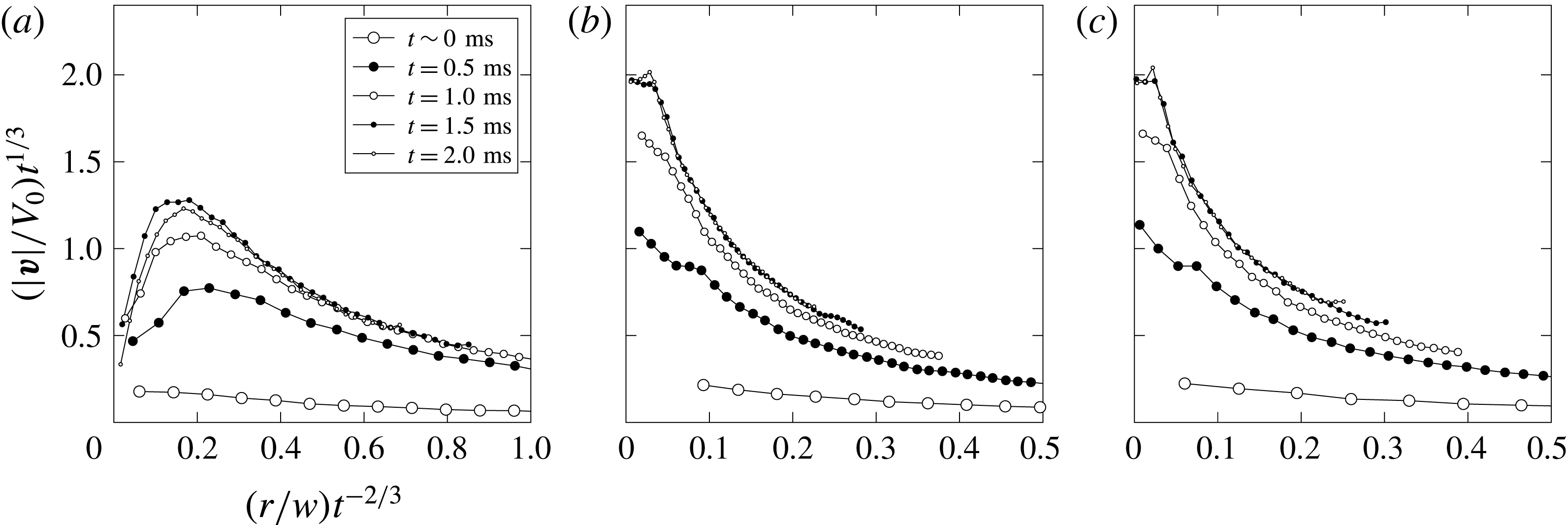
to see if there is indeed a collapse of the data. The results are shown in figure 14, where the data are scaled according to Yakimov’s choice
 $\unicode[STIX]{x1D712}=1/2$
, specifically
 $\boldsymbol{v}\sim r^{-1/2}$
from which
 $\boldsymbol{v}\,t^{1/3}$
and
 $r\,t^{-2/3}$
follow. The scaled data, even after ruling out the earliest curves (for which the uncertainty in time is the largest) and the curves for the largest values of dimensional time, do not support that Yakimov’s scaling is valid, which is explained below.
Scaled velocity profiles for
 $We=90$
(large impact plate,
 $w=25~\text{mm}$
,
 $\unicode[STIX]{x1D707}=1~\text{mPa}~\text{s}$
) and angle
 $\unicode[STIX]{x1D703}$
: (a)
 $0^{\circ }$
, (b)
 $-45^{\circ }$
, (c)
 $-90^{\circ }$
. Scaling is obtained by considering the velocity field to vary as
 $\boldsymbol{v}\sim r^{-\unicode[STIX]{x1D712}}$
, from which we obtain
 $\boldsymbol{v}\,t^{\unicode[STIX]{x1D712}/(1+\unicode[STIX]{x1D712})}$
and
 $r\,t^{-1/(1+\unicode[STIX]{x1D712})}$
with the value of
 $\unicode[STIX]{x1D712}=1/2$
corresponding to Yakimov’s scaling (1.5).

First, it is worth noting that Yakimov (Reference Yakimov1973), who was the first to study the local behaviour of the free interface close to the edge of a flat bottomed cylinder entering water with the aim of understanding the effect of the surrounding air density on the ejecta, developed his scaling based on the simple dimensional argument and the inviscid asymptotics (1.3). Namely, given that the velocity near the plate edge behaves as
 $\boldsymbol{v}\sim r^{-1/2}$
for
 $r\ll w$
and that (naively)
 $\boldsymbol{v}=\text{d}\boldsymbol{r}/\text{d}t$
, Yakimov posited that
 $r/t^{2/3}$
must be a self-similar variable, which in the subsequent studies was tacitly assumed to be valid in the bulk flow as well. Of course, imposing the KJ condition to avoid the singular velocity field and thus modifying the flow field near the plate edge necessarily destroys Yakimov’s argument for his scaling (1.5) based on the singular velocity (1.3). As recently pointed out (Krechetnikov Reference Krechetnikov2014b
), the assumption that
 $\boldsymbol{v}=\text{d}\boldsymbol{r}/\text{d}t$
, which Yakimov’s scaling is based upon, is the equation for pathlines (a Lagrangian concept) and therefore application of Yakimov’s scaling deduced from Lagrangian considerations to Eulerian variables is not appropriate, since these two descriptions – Lagrangian and Eulerian – generally do not coincide in the unsteady case to which our problem belongs. However, at the interface, which is a material line, each point moves with the same velocity as the fluid in view of the kinematic boundary condition (1.4) and thus one arrives at the Yakimov scaling (1.5), which explains why its comparison with experimental measurements of the interfacial motion (Peters et al.
Reference Peters, van der Meer and Gordillo2013) is in reasonable agreement.
The self-similar variables introduced by Yakimov were adopted in a number of recent studies (Oliver Reference Oliver2002; Iafrati & Korobkin Reference Iafrati and Korobkin2004; Peters et al.
Reference Peters, van der Meer and Gordillo2013) and claimed to be tested at the free interface against potential flow numerical simulations (Iafrati & Korobkin Reference Iafrati and Korobkin2008, Reference Iafrati and Korobkin2011) and experimental data (Yakimov Reference Yakimov1973; Iafrati & Korobkin Reference Iafrati and Korobkin2004; Peters et al.
Reference Peters, van der Meer and Gordillo2013), but not against the actual velocity field in the bulk. While it is remarkable that the scaling for the free surface profile
 $y\sim t\,x^{-1/2}$
(which is a simple consequence of
 $\boldsymbol{v}\sim r^{-1/2}$
and
 $y\sim v\,t$
, i.e. arrived at without Yakimov’s scaling) is consistent with what Yakimov’s scaling (1.5) would predict at the free surface, this does not mean that the latter scaling is valid in the bulk, in particular because in the limit
 $t\rightarrow 0$
it does not allow one to recover the inviscid formulation from the NSEs (Krechetnikov Reference Krechetnikov2014b
). Despite the above criticism, the asymptotics
 $\boldsymbol{v}\sim r^{-1/2}$
and Yakimov’s scaling may be observable at the interface for high enough Reynolds and Weber numbers in the intermediate range of distances from the edge
 $\max \{l_{\unicode[STIX]{x1D708}},l_{\unicode[STIX]{x1D70E}}\}\ll r\ll w$
, where
 $l_{\unicode[STIX]{x1D708}}$
and
 $l_{\unicode[STIX]{x1D70E}}$
are the length scales at which viscous and surface tension effects, respectively, prevail (cf. discussion in § 4.2) and thus destroy the solution (1.3).
Lastly, it is notable that, while for
 $r\ll w$
the plate can be seen as semi-infinite, equation (1.3) illustrates how taking this limit (and thus separating spatial scales) does not remove dependence on the corresponding remote scale: near the plate edge,
 $r\ll w$
, the solution is self-similar, but the dependence on the disparate scale
 $w$
does not vanish – this behaviour comes from the elliptic character of the problem in which all boundary conditions affect the solution everywhere (Krechetnikov Reference Krechetnikov2014a
,Reference Krechetnikov
b
), which is different from, say, the Prandtl boundary layer on semi-infinite plate due to the parabolic character of the latter. Therefore, from the point of view of intermediate asymptotics (Barenblatt Reference Barenblatt1996), the self-similarity observed in (1.3) is of the second kind, i.e. when the comparatively large parameter
 $w\gg r$
still has an
 $O(1)$
effect on the solution.
4 Results: free surface evolution
4.1 Previous efforts
In contrast to the lack of previous efforts to measure velocity fields in the flat bottomed impacts, free surface deflection measurements were attempted many times starting with the work of Yakimov (Reference Yakimov1973) on the impact of a cylinder end (same as a circular disk impact), though with no time stamps, which complicates any comparison against theory, albeit only heuristically (Iafrati & Korobkin Reference Iafrati and Korobkin2004); Lin & Shieh (Reference Lin and Shieh1997a ,Reference Lin and Shieh b ) on cylinder impact, who provided only qualitative profiles; Greenhow & Lin (Reference Greenhow and Lin1983) on wedge and cylinder impact; and Peters et al. (Reference Peters, van der Meer and Gordillo2013) on a round disk impact who compared a single point of the ejecta profile with numerical simulations after introducing heuristic time shifts and neglecting a substantial portion of the ejecta. The bottom line is that no high fidelity data sets exist in the literature, which in part is due to the difficulty at visualizing and accurately measuring the velocity field and free surface deformations, especially in the highly singular near-edge region. These are overcome in our experimental approach.
4.2 Origin of ejecta and general observations
To understand the origin of ejecta in the water impact, it is instructive first to think in terms of mass conservation in a compressible impact. Once the plate hits the surface, at time
 $t>0$
the fluid is affected only at the distance
 $c_{0}\,t$
. Two effects are happening at the same time: fluid is being both compressed and displaced. Since the affected volume
 $2\,c_{0}\,t\,w$
is finite, as illustrated in figure 1(c), one can estimate the displaced volume as
 $2\,V_{0}\,t\,w$
, which based on mass conservation is approximately equal to the volume lost through ejecta
 $2\,V_{e}\,t\,c_{0}\,t$
, thus giving
 $V_{e}\sim V_{0}\,w/(c_{0}\,t)$
for short times. This qualitative mass conservation consideration, neglecting the liquid compression, suggests the following: the closer the time to the impact event the higher the ejecta speed, which is consistent with many observations of various impact phenomena; the wider the plate (or the blunter the impacting object), the faster the ejecta; the more compressible/stretchable the liquid (smaller
 $c_{0}$
) the smaller the affected volume and hence faster the ejecta. Of course, for small enough
 $c_{0}$
one has to take into account the compression of the displaced liquid, which in turn will affect the mass lost through ejecta. In the limit of an incompressible flow,
 $c_{0}\rightarrow +\infty$
, the same consideration applies with the only difference that the affected fluid volume is, strictly speaking, infinite because of the infinite speed of sound propagation. In reality, however, the affected volume is still finite, which can be seen from the decay rate of the velocity field:
 $u-\text{i}\,v=\text{d}f/\text{d}z\sim (w/z)^{2}$
for
 $|z|\rightarrow \infty$
. This, in fact, explains why the added mass even in the incompressible impact is finite (Lavrentiev & Schabat Reference Lavrentiev and Schabat1967).
From the dynamical point of view, in the inviscid potential approximation the constancy of the pressure at the fluid interface implies that the pressure gradient
 $\unicode[STIX]{x1D735}p$
must be orthogonal to the interface and so is the fluid particle acceleration as well (Logvinovich Reference Logvinovich1973). This is consistent with the solution (1.2): the flow must turn around the plate edge and the associated (near) singular velocity field is crucial for the existence of the ejecta. To appreciate that, let us look at the mechanism behind the ejecta evolution for
 $t\rightarrow 0+$
, i.e. when the viscous boundary layer has not had time to develop yet and the interface (with surface tension) is still almost undisturbed. Then we can linearize the governing equations around the flat interface
 $y=0$
, so that the initial condition on the interface is
 $\unicode[STIX]{x1D702}|_{t=0}=0$
, and arrive at
 $$\begin{eqnarray}y=0:\unicode[STIX]{x1D702}_{t}=\unicode[STIX]{x1D719}_{y}\quad \text{and}\quad \unicode[STIX]{x1D719}_{t}=-g\,\unicode[STIX]{x1D702}+(\unicode[STIX]{x1D70E}/\unicode[STIX]{x1D70C})\unicode[STIX]{x1D702}_{xx}.\end{eqnarray}$$
It is known from water wave theory that this system leads to the wave-type equation for
 $\unicode[STIX]{x1D702}$
. Given that the velocity field (1.3) is singular at
 $x\rightarrow 0$
, the first of equations (4.1) provides the second initial condition
 $\unicode[STIX]{x1D702}_{t}|_{t=0}\sim x^{-1/2}$
, i.e. it works as a significant initial kick to the interface at the plate edge, which then grows, propagating to the right. Following from (4.1) the qualitatively equivalent wave equation
 $\unicode[STIX]{x1D702}_{tt}=c^{2}\unicode[STIX]{x1D702}_{xx}$
, where
 $c$
is proportional to
 $\unicode[STIX]{x1D70E}^{1/2}$
for short wavelengths corresponding to the early times of ejecta evolution, augmented with the natural boundary condition
 $\unicode[STIX]{x1D702}(t,0)=0$
at the plate edge produces a solution:
 $$\begin{eqnarray}\unicode[STIX]{x1D702}(t,x)=\left\{\begin{array}{@{}cc@{}}\displaystyle \frac{1}{2c}\int _{x-ct}^{x+ct}\unicode[STIX]{x1D713}(s)~\text{d}s=\sqrt{x+c\,t}-\sqrt{x-c\,t}, & x>ct,\\ \displaystyle \frac{1}{2c}\int _{ct-x}^{ct+x}\unicode[STIX]{x1D713}(s)~\text{d}s=\sqrt{ct+x}-\sqrt{ct-x}, & \text{and }x<ct,\end{array}\right.\end{eqnarray}$$
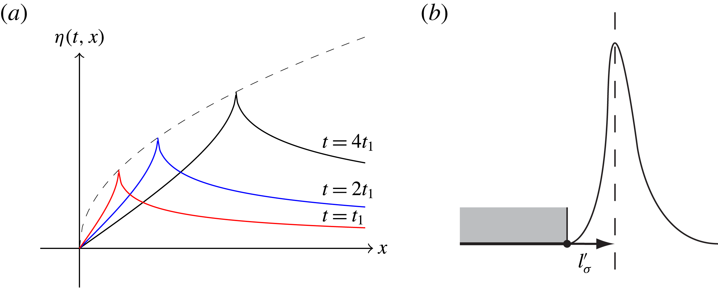
which is plotted in figure 15(a) showing that the ejecta tip propagates along the envelope
 ${\sim}x^{1/2}$
shown with dashed curve. From this simple qualitative analysis we conclude that without surface tension the ejecta would not propagate to the right and, in fact, it would be infinitely extended as
 $\unicode[STIX]{x1D702}\sim x^{-1/2}$
following the distribution of the initial velocity (1.3). Thus, surface tension has a regularizing effect. Of course, since the actual velocity distribution is not as singular as
 $r^{-1/2}$
, cf. § 3.3, the ejecta tip will no longer be a cusp.
On the effects of surface tension: (a) origin of ejecta, (b) determining
 $l_{\unicode[STIX]{x1D70E}}^{\prime }$
.

The dispersion relation corresponding to (4.1) for a monochromatic interfacial wave
 $\unicode[STIX]{x1D702}\sim \text{e}^{\text{i}(k\,x-\unicode[STIX]{x1D714}t)}$
in the deep water limit (to which our case belongs)
 $$\begin{eqnarray}\unicode[STIX]{x1D714}^{2}=g\,k+(\unicode[STIX]{x1D70E}/\unicode[STIX]{x1D70C})\,k^{3},\quad k=2\unicode[STIX]{x03C0}/\unicode[STIX]{x1D706},\end{eqnarray}$$
in the short wave limit
 $\unicode[STIX]{x1D706}\rightarrow 0$
gives the velocity
 $$\begin{eqnarray}v_{g}=\text{d}\unicode[STIX]{x1D714}/\text{d}k={\textstyle \frac{3}{2}}\sqrt{\unicode[STIX]{x1D70E}/\unicode[STIX]{x1D70C}}k^{1/2},\end{eqnarray}$$
which is calculated here as a group velocity since the ejecta at early times is represented by a spectrum of wavelengths in view of its singular character. In the absence of viscosity, at very early times the surface tension alone (since gravity is irrelevant) dictates the linear wave-like evolution of the interface as per the above discussion. Since gravity is irrelevant at early times and the interface deflects in the linear regime, there is no time-independent surface tension length scale – as a result, similar to the viscous diffusion problem, the characteristic surface tension length scale
 $l_{\unicode[STIX]{x1D70E}}$
necessarily depends on time as follows from (4.3):
 $$\begin{eqnarray}l_{\unicode[STIX]{x1D70E}}\sim 2\unicode[STIX]{x03C0}(\unicode[STIX]{x1D70E}/\unicode[STIX]{x1D70C})^{1/3}t^{2/3},\end{eqnarray}$$
which is due to the hyperbolic (non-dissipative) character of surface tension effects – the initial ejecta is singular and consists of many wavelengths, with
 $l_{\unicode[STIX]{x1D70E}}$
being the characteristic one. Since
 $l_{\unicode[STIX]{x1D70E}}\sim t^{2/3}$
versus
 $l_{\unicode[STIX]{x1D708}}\sim t^{1/2}$
, the viscous effects propagate faster at short times until
 $t^{\ast }\sim \unicode[STIX]{x1D708}^{3}(\unicode[STIX]{x1D70C}/\unicode[STIX]{x1D70E})^{2}$
and
 $l_{\unicode[STIX]{x1D70E}}^{\ast }\sim \unicode[STIX]{x1D707}^{2}/(\unicode[STIX]{x1D70C}\,\unicode[STIX]{x1D70E})$
, after which surface tension takes over and there appears a time-independent length scale.
Another length scale emerges when the associated capillary pressure becomes of the same order as viscous stresses – the singular velocity (1.3) tends to stretch the interface, but the latter is attached to the plate edge, so there is a small portion of the interface with high curvature at the plate edge, see figure 15(b). If near the edge
 $\boldsymbol{v}\sim V_{0}(w/r)^{1/2}$
as predicted by inviscid theory (1.3) defining the outer potential flow, then capillary pressure can balance the viscous stresses at the critical distance
 $l_{\unicode[STIX]{x1D70E}}^{\prime }$
determined from
 $$\begin{eqnarray}\unicode[STIX]{x1D707}V_{0}\sqrt{w/r^{3}}\sim \unicode[STIX]{x1D70E}/r\Rightarrow l_{\unicode[STIX]{x1D70E}}^{\prime }\sim \unicode[STIX]{x1D707}^{2}V_{0}^{2}w/\unicode[STIX]{x1D70E}^{2}=l_{\unicode[STIX]{x1D70E}}^{\ast }\,We,\end{eqnarray}$$
e.g. for
 $V_{0}=1~\text{m}~\text{s}^{-1}$
and water
 $l_{\unicode[STIX]{x1D70E}}^{\prime }=10^{-5}~\text{m}$
, but for water–glycerol (58 %) we get
 $l_{\unicode[STIX]{x1D70E}}^{\prime }=1~\text{mm}$
. Given that the observed velocity (figure 10) is less singular than
 $\boldsymbol{v}\sim r^{-1/2}$
, the actual critical distance
 $l_{\unicode[STIX]{x1D70E}}^{\prime }$
could be larger than predicted above.
To set terminology to be used in the following discussion, we remind the reader that since the near-edge velocity asymptotics is
 $\boldsymbol{v}\sim r^{-1/2}$
for
 $r\ll w$
, the theoretically expected free surface profile should scale as
 $y\sim x^{-1/2}$
, which we call an outer profile in this near-edge region. Because the outer profile clearly does not meet the plate edge and thus real physical effects interfere to modify the free surface close to the plate edge, we will call the latter part of the free surface an inner surface profile. As shown in Krechetnikov (Reference Krechetnikov2014b
) the scaling here is
 $y\sim x^{3/2}$
valid in the Stokes approximation. Finally, away from the plate edge,
 $r\gg w$
, the velocity should scale as
 $\boldsymbol{v}\sim r^{-2}$
as follows from (1.2) and therefore the free surface should scale as
 $y\sim x^{-2}$
in this far-field region.
4.3 Experimental procedure
The fact that the above theoretical free surface scalings intended to be tested here are valid for
 $\widetilde{t}=t/\unicode[STIX]{x1D70F}\ll 1$
, where
 $\unicode[STIX]{x1D70F}=w/V_{0}$
is a characteristic time introduced before, leads to a challenge from an experimental standpoint, as resolving the ejecta at both short times (requiring high-speed imaging) and over small distances (requiring high magnification) is not straightforward when both
 $x/w$
and
 $t/\unicode[STIX]{x1D70F}$
are required to be small. Thus, we have to choose
 $w$
to be as large and
 $V_{0}$
as small as possible. The later requirement in turn leads to smaller deflections of the surface profile which are more difficult to resolve. A further condition that limits the time for observation of the surface profile evolution is the shallow depth of penetration
 $h$
of the impact plate. Considering
 $t_{h}=h/V_{0}$
to be this time scale, we find that our observations are restricted to a dimensionless time given by
 $\widetilde{t}_{h}=h/w$
. Taking these conditions into account, we chose
 $w=25~\text{mm}$
,
 $h=1~\text{mm}$
and
 $V_{0}=0.25~\text{m}~\text{s}^{-1}$
for detailed profile measurements. Liquids 1, 4 and 6 were used in these experiments so that for a fixed impact speed the Weber number does not vary much. However, significant changes in liquid viscosity produce a wide range of Reynolds numbers.
A high-speed camera (Phantom v5.2) with a macro lens and an extension tube was used to image the surface in the neighbourhood of
 $0<x\leqslant 2.5~\text{mm}$
. In order to obtain a reasonable resolution for this field of view we were limited to frame rate of
 $5000~\text{fps}$
, i.e.
 $\unicode[STIX]{x0394}t=0.2~\text{ms}$
between each pair of still images. The result is that we can image the surface profile within the distances
 $0<x/w\leqslant 0.1$
from the plate edge, with
 $\unicode[STIX]{x1D70F}\sim 100~\text{ms}$
so that these profiles correspond to dimensionless times in the range of
 $\widetilde{t}=0.002{-}0.04$
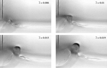
producing 5–10 useful images for each experiment due to the rapid rise in the free surface after impact. A representative sequence of images is shown in figure 16. Surface profiles are extracted from the high-speed movie frames with the origin of the
 $xy$
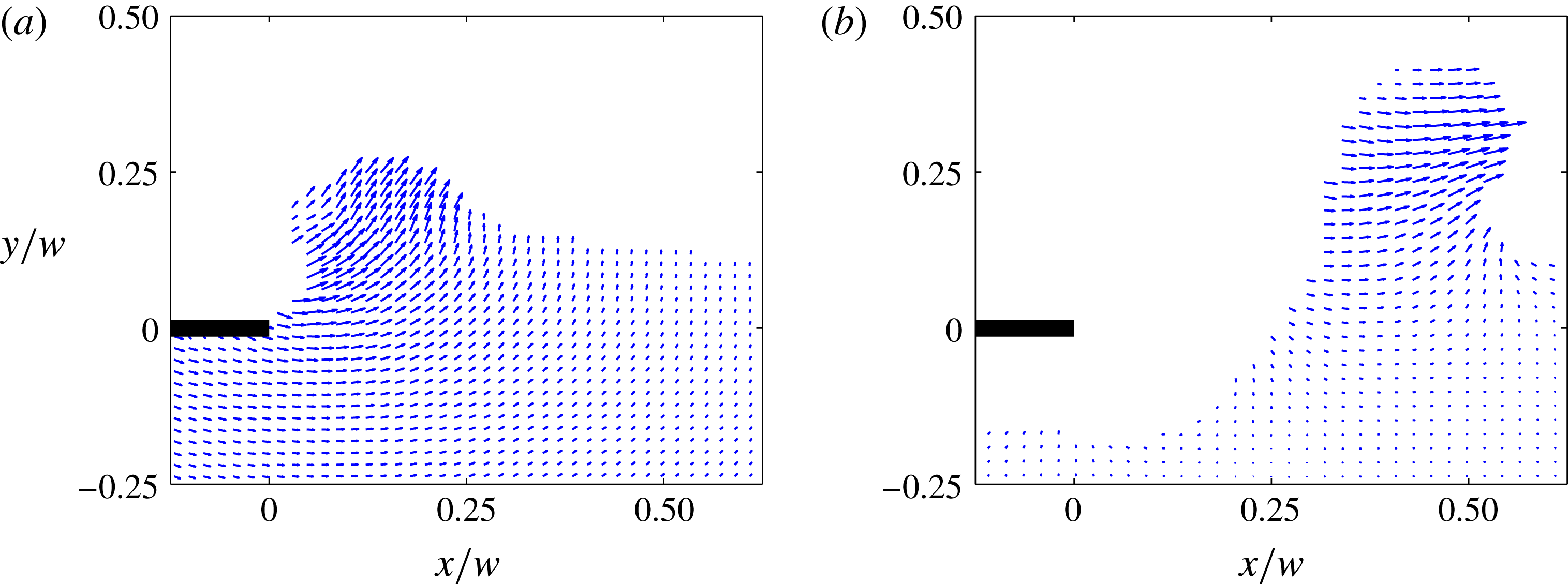
coordinate system corresponding to the location of the impact plate corner when it first makes contact with the liquid surface. The improved optical access (Appendix) is not only useful for bright-field imaging with the high-speed camera, but also allows PIV measurements within the otherwise-concealed portions of the ejected liquid (figure 17). As opposed to the inviscid theory (1.2), which gives no
 $x$
-component of velocity at the free interface as per (1.3) for
 $\unicode[STIX]{x1D703}=0$
, the ejecta clearly has the horizontal velocity as well, which is due to non-zero surface tension as per the discussion in § 4.2.
Ejecta evolution near the edge of the impact plate imaged using a high-speed camera (water,
 $w=25~\text{mm}$
and
 $V_{0}=0.28~\text{m}~\text{s}^{-1}$
) at shallow depth of focus and long distance focal length in order to image the free surface in the middle section of the impactor plate away from the tank walls. Each photo shows a region near the plate edge
 $5~\text{mm}$
wide and
 $3~\text{mm}$
tall. The dark line near the left-hand edge is a vertical scratch in the aluminium impact plate used to focus the camera and locate the corner. This scratch does not extend to the bottom edge of the plate to avoid any influence on the shape of the ejecta.

Improved optical access using the reduced wall–plate gap enables PIV measurements within the ejected liquid. Representative images of PIV inside the ejected liquid for two different times corresponding to the case of
 $w=10~\text{mm}$
and
 $V_{0}=0.3~\text{m}~\text{s}^{-1}$
: (a) before abrupt deceleration of the plate (
 $t=2.5~\text{ms}$
), and (b) after abrupt deceleration of the plate (
 $t=12.5~\text{ms}$
), cf. figure 3(b), and during air pocket formation. The lengths of the largest vectors correspond to velocity magnitudes of (a)
 $0.5~\text{m}~\text{s}^{-1}$
and (b)
 $0.4~\text{m}~\text{s}^{-1}$
. The empty region beneath the plate in (b) is void of velocity vectors because of the air pocket in that region.

4.4 Self-similarity analysis
One of the key questions we intended to address in this work is whether the surface profiles are self-similar, although now obviously not following Yakimov’s scaling
 $(x,y)\sim t^{2/3}$
. An example of extracted profiles is provided in figure 18(a) for the impact on water at four dimensionless times such that the condition
 $\widetilde{t}<h/w\ll 1$
is satisfied. As anticipated, despite the fact that the location of the plate edge changes as the plate penetrates further into the liquid, the depth of penetration stays considerably smaller than the peak elevation of the ejecta due to the rapid growth of the latter. Here, in figure 18(a), the data have been normalized by the plate width to demonstrate that the profiles are confined within a small region near the plate edge, i.e.
 $x/w\leqslant 0.1$
. The surface profiles appear similar in structure, albeit scaled with time, reminiscent of the Yakimov (Reference Yakimov1973) qualitative comment regarding his own photographs. The location of maximum height of the ejected liquid is shown as a white dot. We can extract the
 $x_{m}$
and
 $y_{m}$
coordinates of this peak point for each profile in the complete sequence of images of which only four are given in figure 18(a). When these peak coordinates are plotted as a function of time, they appear to suggest a power-law scaling
 $(\widetilde{x}_{m},\widetilde{y}_{m})\rightarrow (x_{m},y_{m})\,t^{\unicode[STIX]{x1D6FC}}$
with an exponent
 $\unicode[STIX]{x1D6FC}$
somewhere in between
 $2/3$
(corresponding to Yakimov’s scaling) and
 $\text{1}$
, see inset in figure 18(b).
Analysis of surface profiles for water impact under the conditions of
 $w=25~\text{mm}$
,
 $h=1~\text{mm}$
and
 $V_{0}=0.25~\text{m}~\text{s}^{-1}$
. (a) Surface profiles in the physical space for water impact. The white dot identifies the location of maximum height of the profile. Only a select number of images are presented for illustrative purposes. (b) Collapsed surface profiles in the scaled space for the least-square fit time scaling exponent
 $\unicode[STIX]{x1D6FC}\simeq 0.75$
. The axes are the scaled dimensions
 $\widetilde{x}$
and
 $\widetilde{y}$
(taken from a
 $2.5~\text{mm}\times 2.5~\text{mm}$
region). Inset shows scaling of the peaks of the surface profiles. The
 $x$
and
 $y$
location of the maximum height of each profile for the impact conditions of (a) is plotted as a function of time. The data appear to follow a power-law trend with an exponent between
 $2/3$
(solid line) and 1 (dashed line).

Rather than to scale the coordinates of the peak point alone, we can also find a least-square fit scaling exponent
 $\unicode[STIX]{x1D6FC}$
for the entire (including inner and outer) measured profile illustrated in figure 18(b) with the
 $x$
and
 $y$
coordinates transformed as
 $$\begin{eqnarray}(x/w)\rightarrow (x/w)(\unicode[STIX]{x1D70F}/t)^{\unicode[STIX]{x1D6FC}},\quad (y/w)\rightarrow (y/w)(\unicode[STIX]{x1D70F}/t)^{\unicode[STIX]{x1D6FC}},\end{eqnarray}$$
where
 $\unicode[STIX]{x1D70F}=w/V_{0}$
as before. The best collapse is produced using
 $\unicode[STIX]{x1D6FC}=0.75$
, consistent with the scaling of the peaks in the inset of figure 18(b). The fact that the free surface profiles collapse in this self-similar fashion suggests that the velocity field, e.g. in figure 14(a), must collapse as well since the free surface and velocity at it are related by the kinematic condition (1.4): indeed, if the free surface profile is self-similar, this property must be respected by the kinematic boundary condition (1.4) and therefore if
 $(x,f)\sim t^{\unicode[STIX]{x1D6FC}}$
, then necessarily
 $(u,v)\sim t^{1-\unicode[STIX]{x1D6FC}}$
. However, as we saw in figure 14(a), the collapse does not happen with Yakimov’s exponent
 $2/3$
, but rather with a different value of
 $\unicode[STIX]{x1D6FC}$
.
4.5 Further physical observations
Typical surface profiles of the liquid ejected near the edge after impact (plate size
 $w=25~\text{mm}$
). (a) Variable
 $\unicode[STIX]{x1D707}$
: profiles for three values of liquid viscosity (surface tension differences are insignificant). (b) Variable
 $\unicode[STIX]{x1D70E}$
: profiles for two values of surface tension (viscosity differences are insignificant). All profiles correspond to
 $\widetilde{t}=0.01$
. The profiles in (a) are all for the impact velocity
 $V_{0}=0.28~\text{m}~\text{s}^{-1}$
. In (b), the
 $\unicode[STIX]{x1D70E}=72~\text{mN}~\text{m}^{-1}$
data set (water) is repeated from (a), but the
 $\unicode[STIX]{x1D70E}=25~\text{mN}~\text{m}^{-1}$
data set (ethanol) corresponds to
 $V_{0}=0.22~\text{m}~\text{s}^{-1}$
(the lower impact velocity is chosen to match the ejecta height with that for water – this difference in
 $V_{0}$
is not responsible for the difference in shape).

We can extend the above test of scaling to liquids with higher viscosity. Figure 19(a) shows three curves that correspond to the same dimensionless time after impact,
 $\widetilde{t}\simeq 0.01$
. The plot, however, has been left in dimensional form to highlight the differences in spatial dimensions associated with shapes resulting from changes in viscosity. At this magnified field of view we can notice that the shapes of the profiles very near the edge (
 $x\leqslant 0.25~\text{mm}$
) do not seem to vary significantly, unlike portions of the profiles further from the edge. In the neighbourhood of
 $x\simeq 0.5~\text{mm}$
the profiles become much steeper for the more viscous liquids. From figure 19(b) we can see that reducing the surface tension, while holding viscosity fixed, also leads to differences in ejecta profile giving rise to more narrow ejecta. The above observations can be qualitatively explained with the analysis in § 4.2. First, the group velocity
 $v_{g}$
is diverging in the short-wavelength limit (4.4) thus justifying the higher horizontal velocity of the ejecta at early times, cf. inset in figure 18(b) showing that
 $x\sim t^{\unicode[STIX]{x1D6FC}}$
with
 $2/3<\unicode[STIX]{x1D6FC}<1$
and thus
 $\text{d}x/\text{d}t\sim t^{\unicode[STIX]{x1D6FC}-1}\rightarrow \infty$
as
 $t\rightarrow 0$
. As time progresses, the ‘effective’ wavelength of ejecta increases and the gravity takes over with the resulting slower group speed
 $v_{g}=1/2\sqrt{g/k}$
. The hyperbolic character of the interface evolution explains wave steepening in the nonlinear regime in figure 18(a), for example. Higher surface tension naturally leads to smoother (less singular) ejecta and a higher speed of propagation as seen in figure 19(b). Inclusion of viscous dissipation explains the observed slowing down and diffusion (spreading) of the ejecta in figure 19(a).
We have discovered that these differences in the overall shape of the ejecta due to the influence of viscosity and surface tension (figure 19), also affect the power-law exponent that best collapses the ejecta shapes. This behaviour is shown in figure 20 in which each data point represents a best-fit time scaling exponent for a unique impact event. For each liquid, a range of impact speeds was tested resulting in a range of Weber numbers
 $We\leqslant 150$
(and a corresponding range in Reynolds numbers of
 $10<Re\leqslant 15\,000$
). As follows from our quantification of the velocity field in the bulk near the plate edge (§ 3.3), Yakimov’s scaling does not apply for any significant range of
 $r$
. Despite the inevitable experimental errors associated with the accuracy of identifying the free interface in space/time and the standard deviation when collapsing the profiles, there are still noticeable deviations from Yakimov’s exponent.
Time scaling exponent for a range of
 $We$
numbers and liquid viscosities. Values of
 $\unicode[STIX]{x1D6FC}$
were determined using the surface profiles extracted from high-speed images corresponding to
 $\widetilde{t}<1$
. Correspondence of the left-most points for water with Yakimov’s scaling is purely coincidental, which becomes obvious given the left-most point for ethanol and low Weber numbers.

Therefore, we are led to conclude that the free surface self-similarity is not exact, but only approximate, which is easy to understand from the theoretical viewpoint. Indeed, while in the absence of viscosity and surface tension, i.e. when both
 $Re$
and
 $We\rightarrow \infty$
, near the plate edge
 $r/w\ll 1$
one must expect self-similar behaviour of the free surface as there is no independent geometric length scale, at finite
 $Re$
and
 $We$
numbers viscosity and surface tension introduce two independent viscous
 $\unicode[STIX]{x1D707}/(\unicode[STIX]{x1D70C}\,V_{0})$
and surface tension (4.6) length scales, which destroy the self-similarity. Also, for later times, when accelerations become moderate, gravity sets its own length scale
 $V_{0}^{2}/g$
. How gravity and surface tension destroy self-similarity can be seen from the inviscid problem formulation (1.1), where the boundary condition at
 $y=0$
in the semi-infinite plate setting is replaced by
 $$\begin{eqnarray}\unicode[STIX]{x1D719}_{y}=-V_{0},\quad x\leqslant 0\quad \text{and}\quad \unicode[STIX]{x1D719}_{t}+\frac{1}{2}|\unicode[STIX]{x1D735}\unicode[STIX]{x1D719}|^{2}=\frac{\unicode[STIX]{x1D70E}}{\unicode[STIX]{x1D70C}}\frac{\unicode[STIX]{x1D702}_{xx}}{(1+\unicode[STIX]{x1D702}_{x}^{2})^{3/2}}-g\,\unicode[STIX]{x1D702},\quad x>0\end{eqnarray}$$
together with the kinematic condition (1.4). Application of the affine transformation to both independent and dependent variables shows absence of self-similarity when either
 $\unicode[STIX]{x1D70E}\neq 0$
or
 $g\neq 0$
. In particular, the presence of surface tension leads to existence of capillary waves, e.g. in figure 13(a,b), destroying self-similarity. This is similar to the experiment of Gekle et al. (Reference Gekle, van der Bos, Bergmann, van der Meer and Lohse2008) on dragging a smooth finite-length cylinder through a water surface to create a cavity, the surface of which experiences ripples (capillary waves) originating from the cavity corner point as the cylinder top passes the water surface.
Free surface profiles with the
 $\unicode[STIX]{x1D707}=1000~\text{mPa}~\text{s}$
fluid – testing the near-edge power law
 $y\sim x^{3/2}$
(solid) when the apparent angle at which the interface departs the plate edge is
 ${\sim}0^{\circ }$
: (a) profiles in the physical space, (b) collapsed profiles in the scaled space with inset showing near-edge power-law asymptotics on the logarithmic scale. Note that in panel (a) the
 $x$
and
 $y$
-scales are not equal and the inset in panel (b) contains extra profiles for intermediate times
 $t=3,5,7~\text{ms}$
marked by empty circles; symbols for other times in panel (b) are the same as in panel (a). Outer profiles are shown to decay a bit faster than
 $y\sim x^{-1/2}$
(dashed).

Testing the far-field surface profile power law
 $y\sim x^{-2}$
(solid) with the
 $\unicode[STIX]{x1D707}=1~\text{mPa}~\text{s}$
fluid. (a) Profiles in the physical space. (b) Far-field profiles collapsed in the logarithmic space. Note that in panel (b) the outer profiles are collapsed with
 $\unicode[STIX]{x1D6FC}=1.5$
while the inner ones are not, thus indicating that the corresponding scaling time exponents
 $\unicode[STIX]{x1D6FC}$
are different.

To complete our discussion of the free surface evolution for early times near the edge, we use the measured profiles to determine how the free surface deflection
 $y$
scales with position
 $x$
. For the expected scaling
 $y\sim x^{-1/2}$
of the outer profile (see § 1.2), while in the case of the
 $\unicode[STIX]{x1D707}=10^{3}~\text{mPa}~\text{s}$
fluid the scaling exponent is indeed close to
 $-1/2$
, as follows from the inset in figure 21(b), this is purely coincidental. For example, in the case of impact on water shown in figure 18, the corresponding exponent is
 $-1.6$
, i.e. the profile decays much faster – this is the consequence of the fact that the scaling (1.3) for the velocity field near the plate edge is not observed, as discussed in § 3.3. To test the inner profile scaling for the Stokes region (Krechetnikov Reference Krechetnikov2014b
), we used the
 $\unicode[STIX]{x1D707}=10^{3}~\text{mPa}~\text{s}$
fluid so that the boundary layer thickness is of the order of
 $l_{\unicode[STIX]{x1D708}}=1{-}3~\text{mm}$
for the experimental conditions in figure 21. From the inset in figure 21(b) we can see that the inner surface profile in the Stokes approximation indeed scales as
 $y\sim x^{3/2}$
in accordance with the prediction by Krechetnikov (Reference Krechetnikov2014b
). Finally, we tested the far-field free surface profiles: figure 22 shows an example of collapsing profiles measured on a scale comparable to or larger than the plate width in figure 22(a). Clearly, as per figure 22(b), the profiles indeed collapse at far-field distances, but with the self-similarity exponent different from that for the near-edge profile (the data to the left in figure 22(b) do not collapse). An important observation is the rate of decay of these profiles in the far-field region
 ${\sim}(x/w)^{-2}$
(shown with solid line) in accordance with the prediction from the complete inviscid theory (1.2).
5 Results: air entrapment
5.1 Previous efforts
The air trapping upon impact was mentioned in early experimental studies on water impact (Chuang Reference Chuang1966; Verhagen Reference Verhagen1967) and continues to be the subject of more recent works, particularly as the phenomenon is important for correcting the dynamic loads experienced by objects upon impact. While Chuang (Reference Chuang1966) studied plate impact and observed air trapping indirectly via bubble formation after the impact, Verhagen (Reference Verhagen1967), also in the plate impact experiments, observed air trapping directly, but no quantitative measurements were conducted. Ermanyuk & Gavrilov (Reference Ermanyuk and Gavrilov2011), who studied qualitatively air trapping in the disk impact, showed that air trapping occurs regardless of the curvature of the solid impactor bottom, whether it be concave or convex (though still sufficiently small). Only in recent years was air trapping studied quantitatively by Thoroddsen, Etoh & Takehara (Reference Thoroddsen, Etoh and Takehara2003) in the liquid drop impact on a liquid surface, by Marston, Vakarelski & Thoroddsen (Reference Marston, Vakarelski and Thoroddsen2011) and Hicks et al. (Reference Hicks, Ermanyuk, Gavrilov and Purvis2012) in the impact of a rigid sphere on liquid, and by Liu, Tan & Xu (Reference Liu, Tan and Xu2013) in the liquid drop impact on a solid surface. However, no measurements were done for air entrapment in the rectangular plate impact – the classical problem in which the air cushioning effect was originally observed (Chuang Reference Chuang1966).
The trapped circular sheets of air investigated by Thoroddsen et al. (Reference Thoroddsen, Etoh and Takehara2003) and Marston et al. (Reference Marston, Vakarelski and Thoroddsen2011) were shown to retract to form an air bubble from which the volume of trapped air could be estimated. Retraction rates, during the stage when the sheets of air are relatively flat, were found to be well described by a simplified inertial retraction model developed by Thoroddsen et al. (Reference Thoroddsen, Etoh and Takehara2003) and Marston et al. (Reference Marston, Vakarelski and Thoroddsen2011), in which the behaviour of the retracting air sheet after the abrupt initial retraction is believed to be dictated by a competition between the inertia of the sheet rim and surface tension forces acting on it (Taylor Reference Taylor1959; Culick Reference Culick1960), for low viscosity fluids. The resulting retraction rate is determined by the thickness of the air layer which changes with time during retraction, but can be accounted for by conservation of volume. A similar treatment has been provided to describe the retraction of low viscosity droplets initially flattened by impact (Bartolo, Josserand & Bonn Reference Bartolo, Josserand and Bonn2005). The above studies of trapped air retraction also found that the air volume increases with impacting sphere diameter, but decreases with (increasing) impact speed. Hicks et al. (Reference Hicks, Ermanyuk, Gavrilov and Purvis2012) observed the same general trends for large-radius spherical segment impactors. While the air trapping phenomenon is far from being fully understood – especially the effects of viscosity, surface tension, and compressibility – certain progress has been made with formal modelling: an account of previous studies is given by Wilson (Reference Wilson1991).
5.2 On the physics of air entrapment
As noted by von Karman (Reference von Karman1929), plate impact in the absence of air necessitates taking into account compressibility, even when the impact velocity
 $V_{0}$
is negligible compared to that of sound
 $c_{0}$
in the liquid phase, because the flat plate gets in contact with the liquid surface at more than one point simultaneously with the resulting hammering pressure (coinciding with the pressure variation in a plane acoustic wave)
 $$\begin{eqnarray}\unicode[STIX]{x0394}p=\unicode[STIX]{x1D70C}\,c_{0}V_{0},\end{eqnarray}$$
which was also derived rigorously by Galin (Reference Galin1947). However, it was found experimentally by Chuang (Reference Chuang1966) that the presence of air and the resulting trapping of air reduced the impact pressure predicted by formula (5.1) thus diminishing the effect of liquid compressibility, which justifies the term ‘air cushioning’. This fact is consistent with the observations in figure 4(a) that indeed liquid compressibility can be neglected as the depth of the noticeably disturbed fluid, i.e. where the velocity field is established, is of the order of
 $5~\text{mm}$
as opposed to
 $5~\text{cm}$
based on the acoustic estimate
 $c_{0}\,\unicode[STIX]{x0394}t$
for the conditions in that figure. Hence, here we are dealing with the hydraulic stage only.
With reference to figure 1(a), the basic mechanism behind air trapping is as follows. First, Bernoulli’s equation suggests that when the plate approaches the water surface, the peak of the pressure is at the plate centre as the air has a stagnation point there, which results in the largest deflection (dimple) and depresses the free surface causing it to rise away from the centre. This effect is enhanced by the fact that near each of the plate edges the velocity of the escaping air is at its maximum, which lowers the pressure and thus the water surface there rises even more resulting in the first contact with the plate near the corners. Once the air gap decreases, the air velocity in the throat approaches the speed of sound (in air) and thus, as envisaged by Wilson (Reference Wilson1991) with reference to Verhagen (Reference Verhagen1967), the air flow may ‘choke’, i.e. the air speed cannot increase beyond that of sound and hence the air mass flow rate cannot increase. Verhagen (Reference Verhagen1967) further suggested that two shock waves would then form and propagate from the plate edges towards the plate centre, as sketched in figure 1(a). However, as opposed to the standard flow choking phenomena occurring due to the decreasing ambient (downstream) pressure while the upstream pressure is fixed (Loitsyanskii Reference Loitsyanskii1966) – namely, once the flow speed at the throat reaches the sound speed, no changes downstream can affect the flow behaviour upstream – we deal with the situation when it is the upstream pressure (in the gap) that increases thus making it possible to surpass the sound speed in the throat, which should, however, now be at minimum according to the steady nozzle flow theory. The unsteadiness of the collapsing throat (and hence nozzle) in our case may, nevertheless, be responsible for the flow choking phenomena as we allude to in § 5.3. Similarly, when a solid object impacts on a liquid forming a cavity, an air jet is pushed out, necessarily attaining supersonic speeds upon closing (Gekle et al. Reference Gekle, Peters, Gordillo, van der Meer and Lohse2010).
Frames from an impact event sequence filmed with a high-speed camera (water,
 $w=10~\text{mm}$
,
 $V_{0}=0.1~\text{m}~\text{s}^{-1}$
). The motion of the air phase is visualized using dry ice fog above the liquid surface (dark grey). (a) As the plate descends prior to impact, air beneath the plate is driven out. The horizontal component of the displaced air velocity increases as the plate–liquid gap decreases. Time between frames is
 $\unicode[STIX]{x0394}t=1~\text{ms}$
with impact at frame 5. (b) Penetration of the plate into the liquid. The air beneath the plate is trapped. Time between frames is
 $\unicode[STIX]{x0394}t=0.1~\text{ms}$
. (c) Air pocketing after abrupt deceleration of the plate. Although difficult to visualize, there is air flow into the growing pocket. Also the air layer beneath the plate retracts forming a cavity at the plate bottom centre. Time between frames is
 $\unicode[STIX]{x0394}t=1~\text{ms}$
.

The flow of air from beneath the impact plate as it approaches the liquid surface can be seen in sequence (a) of figure 23. Here, dry ice fog (dark grey) has been placed into the tank above the water surface. The fog has completely evaporated in the vicinity of the plate giving it the appearance of normal air (light grey). As the plate descends (figure 23
a frames 1 to 4), the air squeezed out from beneath the plate speeds up as can be gleaned from the change in angle of the light grey region. Upon impact and contact with the liquid surface (figure 23
a frame 5), the air flow from beneath the plate ceases. It is interesting to note that the air ‘jet’ in figure 23(a) frame 5 is in the same direction as the subsequent ejecta formed as soon as the plate starts penetrating the liquid phase, see sequence (b). One may call this a coincidence as the physical mechanisms behind the formation of ejecta and the pushed out air are different: the air jet is formed owing to squeezing the gap between the plate and the water surface, while the ejecta appears due to the near-singular velocity field induced in the impacted liquid, cf. the discussion in § 4.2. Nevertheless, at the macroscopic level both the air jet in figure 23(a) frame 5 and the ejecta in (b) depart at almost
 $45^{\circ }$
, which suggests the following way to look at the phenomena. Namely, the air jet appears from a point source at the intersection of two flat dense media interfaces (the vertical side of the impactor plate and the horizontal water surface) and hence the solution must be symmetric with the air jet propagating along the bisectrix. Physically, the air jet follows the bisectrix due to the viscous boundary layer formed in air along the water surface. Next, the subsequent ejecta follows the same bisectrix because the pressure is the lowest along this line based on Bernoulli’s equation (since the air velocity is the highest along the bisectrix). The noticeable motion of the air in sequence (b) is caused by the residual rotational air flow developed prior to impact. On the observed time scale of the liquid ejection, the latter can affect the surrounding air only up to the distance
 ${\sim}\sqrt{\unicode[STIX]{x1D708}_{air}\,\unicode[STIX]{x0394}t}=O(10^{-1})~\text{mm}$
based on the solution of the first Stokes problem, i.e. the effect is negligible and hence most of the air motion in panel (b) is indeed due to the initially displaced air from beneath the plate. Finally, sequence (c) shows development of an air pocket once the plate is abruptly stopped.
Images of entrapment and retraction of a layer of air beneath the plate in the impact on water with
 $w=10~\text{mm}$
,
 $V_{0}=0.5~\text{m}~\text{s}^{-1}$
,
 $h=1~\text{mm}$
. Corresponding front view drawings illustrate the trapping event. (a) Well ahead of impact, the free surface is undeformed. (b) As the plate approaches the surface, the pressure increase needed to force air toward the edge causes the surface to deflect down near the centre of the plate. (c) At the moment of impact the plate makes contact with the deformed liquid surface at its edges. (d) After the abrupt deceleration, the trapped air sheet retracts rapidly at first, followed by a slower retraction (e) and then collection of the air into a cylinder-like ‘line’ that (f) eventually breaks up into bubbles.

A series of representative images and schematic drawings depicting the formation and dynamics of the trapped air layer as seen from beneath a flat plate is shown in figure 24. Although, these images were acquired from impact on water, all the other liquids tested exhibited the same general behaviour. At the start of the plate motion, far from the liquid surface, see figure 24(a), there is no significant deflection of the free surface. Although the location of initial contact in figure 24(b) cannot be accurately measured from the front view images owing to the front and back wall menisci, from the underside of the plate we can observe that no other points of contact are made except for at the plate edge.
During the stage of plate penetration, no dramatic changes to the trapped air layer are observed from below, and the only point of contact with the liquid still appears to be at the plate edge, see figure 24(c). However, when the plate abruptly stops we see that the edge of the trapped air layer retracts rapidly as indicated by the arrows in figure 24(d). With time, this edge continues to retract but at a decreasing rate. The edge of the retracting air layer also appears to form a rim (reminiscent of a growing cylinder-like blob on a retracting liquid sheet). The edge continues to retract until all of the trapped air forms a cylinder-like ‘line’ beneath the centre of the plate, as can be seen in figure 24(e). This air line then breaks up into bubbles owing to an imminent Rayleigh–Plateau instability observed in figure 24(f).
Figure 24(e,f) exhibits a thin line of bubbles observed for low viscosity liquids only (water and ethanol) and formed when the trapped air edge (contact line) first rapidly accelerates, reaching a peak of a very high speed, and then decelerates to a constant low speed, see figure 25(a). Since the bubble formation is not observed at higher viscosities and it is a higher viscosity fluid (liquid) which is displacing the lower viscosity fluid (air), it cannot be caused by viscous fingering (Saffman–Taylor instability). Hence, the only explanation is a Rayleigh–Taylor instability (or its impulsive limit – a Richtmyer–Meshkov instability in view of nearly impulsive accelerations involved). Indeed, figure 24(c) indicates that during the fast retraction regime the trapped air edge is corrugated, which is due to being prone to the Rayleigh–Taylor mechanism. Since the instability is fully developed and hence nonlinear, bubbles may detach from the highly corrugated contact line. The non-symmetry of the bubble formation in figure 24(e–f) is due to the regime when nonlinearity is present, but still weak, which renders bubble separation irregular. For higher impact velocities leading to more vigorous initial acceleration of the trapped air edge (contact line), we observe bubbles on both sides, but, because the instability is fully developed, the appearance of bubbles is no longer in a regular pattern.
Measurements of the air retraction in water for
 $V_{0}=0.5~\text{m}~\text{s}^{-1}$
,
 $h=1~\text{mm}$
and
 $w=5,10,15~\text{mm}$
. (a) Time
 $t=0$
corresponds to the moment of abrupt deceleration of the plate. Each data point is measured from a sequential high-speed movie frame recorded at
 $4100~\text{fps}$
. It is observed that just after the plate stops there is a rapid retraction of the trapped air pocket edge,
 $V_{i}\simeq 20~\text{m}~\text{s}^{-1}$
. This is followed by a slowly decreasing edge retraction speed. A dimensional plot of the inertial retraction model (5.4) for the trapped air dynamics after abrupt deceleration and the initial rapid retraction stage based on the experimental conditions of figure 25 is provided: the solid lines represent the model results, and the dashed lines are to guide the eye to the origin. Direct comparison of the model with the data of figure 25 using a value of
 $C=1$
suggests that inertial retraction can predict the order of magnitude of the velocity, but the physics of the initial retraction process cannot be captured by such a simple model. (b) The image montage for the
 $w=10~\text{mm}$
case in (a) shows that a rim forms at the edge of the retracting pocket and these rims eventually merge to form a ‘line’ of air. Features marked as (1)–(3) in this montage are also marked at the corresponding times in (a).

The stability of the contact line in figure 24(d,e) is in stark contrast to the earlier observations of instability of an inner contact line at the edge of the enclosed air disk formed during impact of a water drop on a solid substrate (Liu et al. Reference Liu, Tan and Xu2013; Li & Thoroddsen Reference Li and Thoroddsen2015) and the impact of a rigid sphere (Hicks et al. Reference Hicks, Ermanyuk, Gavrilov and Purvis2012) or disk (Ermanyuk & Gavrilov Reference Ermanyuk and Gavrilov2011) onto a liquid. We do observe instability of the contact line in the stage of its rapid motion (with acceleration and deceleration and hence ascribable to a Rayleigh–Taylor mechanism) occurring due to the abrupt halt of the plate, which makes our phenomena analogous to the ones considered in the above cited papers. However, once the velocity of the contact line becomes nearly constant (i.e. no significant acceleration), the Saffman–Taylor mechanism stabilizes the contact line since it is more viscous fluid displacing a less viscous one – this is what we observe during the stage of retraction with almost constant velocity, e.g. figure 24(e), before the air line breaks via a Rayleigh–Plateau mechanism. Following the abrupt deceleration of the plate it also becomes apparent that the air is entrained beneath the plate near the edges, which is seen as the dark growing bands indicated with the black arrows in figure 24(d–f) and will be treated separately in § 6.
5.3 Retraction dynamics of the air layer: experiments
The trajectory of the edge of the trapped air layer is recorded for three plate sizes and shown in figure 25 along with a montage of cropped image sections (strips of the centre of each image in the retraction sequence) from which the edge position is measured and which highlights various stages of the retracting air layer evolution. It is apparent from figure 25(a) that, at the time of the impulsive deceleration, (1) the edge rapidly retracts at a speed of the order of
 $V_{i}\equiv 20~\text{m}~\text{s}^{-1}$
(consistent for all three plate sizes) for this particular set of physical conditions. This rapid retraction is then followed by (2) a period of decreasing edge speed toward a two orders of magnitude lower speed,
 $0.2~\text{m}~\text{s}^{-1}$
, with a noticeable rim on the edge of the air sheet until (3) the air layer is completely retracted to form a ‘line’ volume at the centre of the plate, which is half-cylinder-like due to the low Bond numbers at such length scales. Because of the optical access gained by the reduction of the plate–wall gap (Appendix), we can even see the final result of this retraction process in the front view movies (figure 23
c frames 4 and 5). The entire process of trapped air retraction, with the exception of the initial rapid movement, is reminiscent of a retracting liquid sheet (Taylor Reference Taylor1959; Culick Reference Culick1960), a fact to be used in § 5.4.
There are several more interesting features of the trapped air retraction phenomenon that we can quantify. First, we observe that the initial retraction velocity
 $V_{i}$
of the trapped air is a function of the impact velocity
 $V_{0}$
. This is demonstrated in figure 26(a) in which the results for impacts with a water surface are shown for a variety of plate sizes indicating a strong dependence of the initial air retraction velocity on the impact velocity
 $V_{0}$
. A weaker dependence, if any, on the plate size
 $w$
is observed.
The dynamics of air retraction. (a) Measurements of the initial air retraction velocity
 $V_{i}$
for a range of plate widths
 $w$
and
 $h=1~\text{mm}$
in the impact on a water surface indicate a strong dependence of the initial air retraction velocity
 $V_{i}$
on impact velocity
 $V_{0}$
. For the conditions shown,
 $V_{i}\simeq \text{20}\,V_{0}$
. (b) Trapped air edge position for
 $V_{0}=0.5~\text{m}~\text{s}^{-1}$
,
 $h=1~\text{mm}$
and
 $w=10~\text{mm}$
. Substantial increase in fluid viscosity alters the trajectory of the edge of the trapped air layer. Although it does not appear that the rapid initial retraction is affected by the variation of viscosity and surface tension, increasing viscosity causes the later retraction velocity to decrease; also lowering surface tension (ethanol) leads to a delayed retraction.

Second, there is a dependence of retraction velocity
 $V_{i}$
on fluid viscosity, as per figure 26(b), manifesting itself after the initial rapid retraction of the film, which appears to be the same over a substantial range of dynamic viscosities tested. We also note that for the more viscous fluids, the retracting edge of the air film does not form a distinct rim during the course of its retraction (Savva & Bush Reference Savva and Bush2009) in contrast to the observations for water. The effect of lowering surface tension, shown in figure 26(b), is in retarding the retraction at later times, which is expected as it is the surface tension force which pulls the film.
(a) Air layer thickness
 $h_{air}$
estimated from the volume of the trapped air. While there does not appear to be a general trend with impact speed, there is a noticeable dependence on plate width
 $w$
with wider plates trapping more air. All measurements are for water and
 $h=1~\text{mm}$
. (b) Comparison between the hydrodynamic time,
 $t_{h}=h_{air}/V_{0}$
, it takes for the plate to travel over the distance
 $h_{air}$
, and the acoustic time scale,
 $t_{c}=w/c_{air}$
, it takes for the shock wave formed in the narrowed gap between the plate and free surface to travel half-width
 $w$
, cf. figure 1(a). The dashed curve is for
 $t_{c}=t_{h}$
.

Third, while the volume of trapped air exhibits weak dependence on impact velocity
 $V_{0}$
, it is a stronger function of the plate width
 $w$
as shown in figure 27(a) using water as the impacted liquid. We can estimate the volume of trapped air
 $\text{Vol}_{air}$
from the width
 $2\,w_{air}$
of the half-cylinder ‘line’ that forms after retraction of the air layer and then equate to a uniform film of air with a thickness
 $h_{air}$
across the entire plate width
 $2\,w$
. Since compressibility of the trapped air upon impact is negligible for our physical conditions (Hicks et al.
Reference Hicks, Ermanyuk, Gavrilov and Purvis2012), the conservation of the trapped air volume
 $\text{Vol}_{air}$
is used to find
 $h_{air}$
:
 $$\begin{eqnarray}\text{Vol}_{air}\simeq \frac{\unicode[STIX]{x03C0}w_{air}^{2}}{2}\,l\simeq h_{air}\,2\,w\,l\rightarrow h_{air}\simeq \frac{\unicode[STIX]{x03C0}\,w_{air}^{2}}{4\,w}.\end{eqnarray}$$
Similar estimates of trapped air volume are available in the literature, but only for impact on liquid surfaces by disks (Hicks et al. Reference Hicks, Ermanyuk, Gavrilov and Purvis2012), spheres (Marston et al. Reference Marston, Vakarelski and Thoroddsen2011) and liquid droplets (Thoroddsen et al. Reference Thoroddsen, Etoh and Takehara2003). In those instances, the volume of air is observed to decrease with increasing impact velocity, which is expected based on incompressible mass conservation. Instead, in figure 27(a) we see a different trend for flat plates:
 $$\begin{eqnarray}\displaystyle w>w_{c}\Rightarrow h_{air}\downarrow \quad \text{when }V_{0}\uparrow & & \displaystyle\end{eqnarray}$$
 $$\begin{eqnarray}\displaystyle w<w_{c}\Rightarrow h_{air}\uparrow \quad \text{when }V_{0}\uparrow , & & \displaystyle\end{eqnarray}$$
 $t_{h}=h_{air}/V_{0}$
it takes for the plate to travel over the distance
 $h_{air}$
to the acoustic time scale
 $t_{c}=w/c_{air}$
it takes for the shock wave formed in the narrowed gap between the plate and free surface, cf. figure 1(a), to propagate from the gap back to the plate centre. If
 $t_{c}>t_{h}$
, then the air is continuously pushed out with increasing
 $V_{0}$
– see the data for the wide plate in figure 27(a). If, on the other hand,
 $t_{c}<t_{h}$
, then the unsteadiness of the collapsing gap leads to an effect akin to flow choking preventing the air mass flow rate to increase as
 $V_{0}$
increases as can be discerned from the data for narrow plates in figure 27(a). While the details of the mechanism behind the non-monotonic air mass flow rate behaviour are yet to be understood, we merely remark that the unique combination of the geometry and flow parameters in our experiments allows this (likely) compressible flow effect to be observable through the existence of a critical plate width
 $w_{c}$
at which
 $t_{c}\sim t_{h}$
. The plot in figure 27(b) proves that we are indeed in the regime where
 $t_{h}=O(t_{c})$
, but, of course, the
 $O(1)$
coefficient determining the exact transition between the two regimes specified by (5.3) depends on the exact shape of the air layer and other details. As figure 27(a) suggests, the transition happens somewhere in between
 $w=15~\text{mm}$
and
 $w=25~\text{mm}$
. Note that the dependence
 $w_{air}(V_{0})$
or
 $\text{Vol}_{air}(V_{0})$
follows that for
 $h_{air}(V_{0})$
in figure 27(a) because both these quantities are expressed in terms of
 $h_{air}$
, e.g.
 $w_{air}$
equals to
 $\sqrt{4\,w\,h_{air}/\unicode[STIX]{x03C0}}$
and hence is a function of the impact speed
 $V_{0}$
through the dependence of
 $h_{air}$
on
 $V_{0}$
.
5.4 Retraction dynamics of the air layer: model
To confirm that inertia might be the cause of the retraction of the air sheet observed in figure 25(a) after the period of rapid motion of its edge, we can develop a model invoking considerations similar to that by Thoroddsen et al. (Reference Thoroddsen, Etoh and Takehara2003) and Marston et al. (Reference Marston, Vakarelski and Thoroddsen2011), but for the rectangular geometry of our experiments. Taking the velocity of the edge as
 $u=-\text{d}x/\text{d}t$
, relating it to the trapped air thickness
 $u=C\sqrt{\unicode[STIX]{x1D70E}/(\unicode[STIX]{x1D70C}\,h_{air}(x))}$
as in the classical derivation of the Taylor–Culick-type retraction velocity, and using conservation of the trapped air volume
 $\text{Vol}_{air}$
to relate the thickness of the layer
 $\widetilde{h}_{air}(x)$
at any position
 $x$
(for notation see figure 24
d) to the thickness of the initial air layer
 $h_{air}$
, we obtain
 $$\begin{eqnarray}x^{1/2}(t)=x_{0}^{1/2}-\frac{C}{2}\left(\frac{\unicode[STIX]{x1D70E}}{\unicode[STIX]{x1D70C}\,h_{air}\,w}\right)^{1/2}(t-t_{0})\end{eqnarray}$$
in contrast to the exponential decay model of Thoroddsen et al. (Reference Thoroddsen, Etoh and Takehara2003) and Marston et al. (Reference Marston, Vakarelski and Thoroddsen2011) in the circular geometry. In (5.4) we kept the initial edge location
 $x_{0}$
and initial time
 $t_{0}$
as they do not correspond to
 $w$
and
 $0$
, respectively, owing to the initial rapid retraction. The lower limit of
 $x$
, at which equation (5.4) is still valid, is provided by the radius of the eventual air half-cylinder.
The trajectory of the trapped air edge, shown with solid lines figure 25(a), is calculated with (5.4) using the data for
 $h_{air}$
from figure 27(a) and the measured values of
 $x_{0}$
and
 $t_{0}$
from figure 25; note that we shifted the model results to begin after the initially rapid retraction. We plot the model predictions only up to the value of
 $w-x$
equivalent to the static line of air at the end of retraction using a value of
 $C=1$
in equation (5.4) (consistent with the order of magnitude based on available data in the literature), without an attempt to fit it to the data. Nevertheless, this simple model provides the correct magnitude for the location of the retracting sheet edge. But it fails, quite expectedly, to capture details of the transition from the rapid retraction of the edge to the inertial retraction (at early times), and the transition to zero velocity when the rims merge (at later times). A more advanced model would be necessary to account for the inertia that the edge possesses after the rapid initial acceleration, for the drag force that causes a decrease in velocity and for the deceleration experienced toward the end of retraction when rims merge.
Also of interest here is the origin of the rapid initial retraction, a unique feature observed in our experiments, as it seems uncoupled from the later stages characterized by slower retraction speeds separated by two orders of magnitude. If we consider the inertial retraction of the film when the air layer thickness is at its minimum, we would expect that the initial retraction velocity
 $V_{i}$
is of the order of
 $1~\text{m}~\text{s}^{-1}$
. Hence, the inertial mechanism cannot account for the observed magnitude of
 $V_{i}$
and the only obvious cause left is the abrupt deceleration of the flat plate from the impact speed
 $V_{0}$
to zero as per figure 3(b). This abrupt deceleration gives rise to a substantial negative gage pressure established beneath the plate, so that the difference between the lowered pressure at the centreline of the plate and the atmospheric one at the edge is responsible for the impulsive force that drives the rapid initial retraction.
6 Results: air pocketing
6.1 Previous efforts
Finally, air pocketing has not been reported before, as often in the water impact experiments the object penetrates the liquid phase at substantial depths so that there is cavity formation instead (Richardson Reference Richardson1948; Logvinovich & Yakimov Reference Logvinovich, Yakimov, Sedov and Stepanov1973; Glasheen & McMahon Reference Glasheen and McMahon1996; Lee, Longoria & Wilson Reference Lee, Longoria and Wilson1997; Leng Reference Leng2001; Bergmann et al. Reference Bergmann, van der Meer, Gekle, van der Bos and Lohse2009; LeGoff, Quere & Clanet Reference LeGoff, Quere and Clanet2013). This is in contrast to our experiments in which the impactor stops at finite shallow depth, thus replicating sea landing for a certain range of decelerations. Therefore, the mechanism behind the air pocket formation observed in our experiments, cf. figure 1(d), is different from that for the cavities formed at large penetration depths. Since the pocket does not close, we refer to the phenomenon as air pocketing as opposed to entrainment observed in other situations (Prosperetti & Oguz Reference Prosperetti and Oguz1997; Vandre, Carvalho & Kumar Reference Vandre, Carvalho and Kumar2014).
6.2 Dynamics of the entrained air cavity
Since the motion of the impact plate follows that of the solenoid plunger, a penetration depth
 $h$
is set while the plunger is prevented from further motion by the internal mechanical stop. As we see from figure 3(b), the deceleration happens over
 $O(10^{-4})~\text{s}$
, which brings us to the acoustic regime as the characteristic length scale affected by acoustic waves is
 $O(10)~\text{cm}$
, i.e. of the order of our set-up size – hence it is not hydraulic
 ${\sim}\unicode[STIX]{x1D70C}\,V_{0}^{2}=O(10^{3})~\text{Pa}$
, but acoustic pressure
 ${\sim}\unicode[STIX]{x1D70C}\,c_{0}V_{0}=O(10^{5})~\text{Pa}$
(though softened by the trapped air), which is relevant. Since the latter magnitude is comparable to
 $p_{atm}$
, just after the impact plate is abruptly brought to rest by the mechanical stop, we observe the development of the entrained air pocket along the entire length of the plate. A representative series of images of this phenomenon is shown in figure 28. For all liquids tested, this entrained air pocket is produced if the impact velocity is sufficiently large.
Images depicting the evolution of the entrained air region near the edge of the impact plate after it is abruptly decelerated. Conditions for the images:
 $V_{0}=0.64~\text{m}~\text{s}^{-1}$
,
 $h=1~\text{mm}$
and
 $w=10~\text{mm}$
. The pocket appears dark in these images, which is due to the curved air–water interface in the cavity near the front tank wall.

We can also visualize the flow field in the liquid in the vicinity of the air pocket using the PIV system (figure 29). This is done to compare the velocity at the surface of the air pocket with the velocity beneath the plate and that of the ejected liquid. Figure 29 shows three instances in time. For
 $t-t_{1}<0$
, the flow field beneath the plate corresponds to impact and penetration. The ejected liquid near the corner (red) has considerable velocity in excess of the velocity of the fluid directly beneath the plate. After the plate abruptly stops, the pocket begins to develop. Contours of the velocity magnitude suggest that the velocity of the growing pocket depth
 $d(t)$
is small in comparison to that of the ejected liquid which still continues its trajectory. We also note that during the pocket evolution the velocity of the liquid beneath the plate is negligible, indicating that after the abrupt deceleration all the kinetic energy attained by the added mass of liquid initially set into motion after the impact (not including the ejecta liquid) is lost, which is due to the negative pressure impulse, caused by the deceleration, reversing the flow as discussed in § 5. Figure 30 also shows the details of the velocity field around the growing air pocket. At inception, see figure 30(a), the velocity vectors still leave the plate as in the absence of the air pocket, but later on, see figure 30(b,c), the fluid is pushed away from the pocket, as is clearly indicated by the velocity vectors. In what follows we qualitatively and quantitatively describe the evolution of these air pockets and present a simple model to predict their maximum size.
PIV images (top row) and velocity magnitude contour plots (bottom row) before and during the entrained air pocket evolution: (a)
 $t-t_{1}<0$
, (b)
 $t-t_{1}=1~\text{ms}$
, (c)
 $t-t_{1}=10~\text{ms}$
. These images were taken in the impact on water experiments under the conditions of
 $w=10~\text{mm}$
,
 $h=1~\text{mm}$
and
 $V_{0}=0.64~\text{m}~\text{s}^{-1}$
. While these images are provided here for qualitative purposes, all the PIV measurements were taken with the same initial calibration and hence relative magnitudes are consistent. It is apparent that during impact the ejected liquid near the corner is imparted with a considerable velocity (red). After the abrupt deceleration of the plate, the air pocket develops. However, it appears that the speeds associated with the pocket growth are small (blue) compared to the velocity in the ejected liquid. Images are
 $15~\text{mm}$
square. The contour plots appear pixelated, which is a result of the grid size used in the PIV analysis software and masking out the air pocket region.
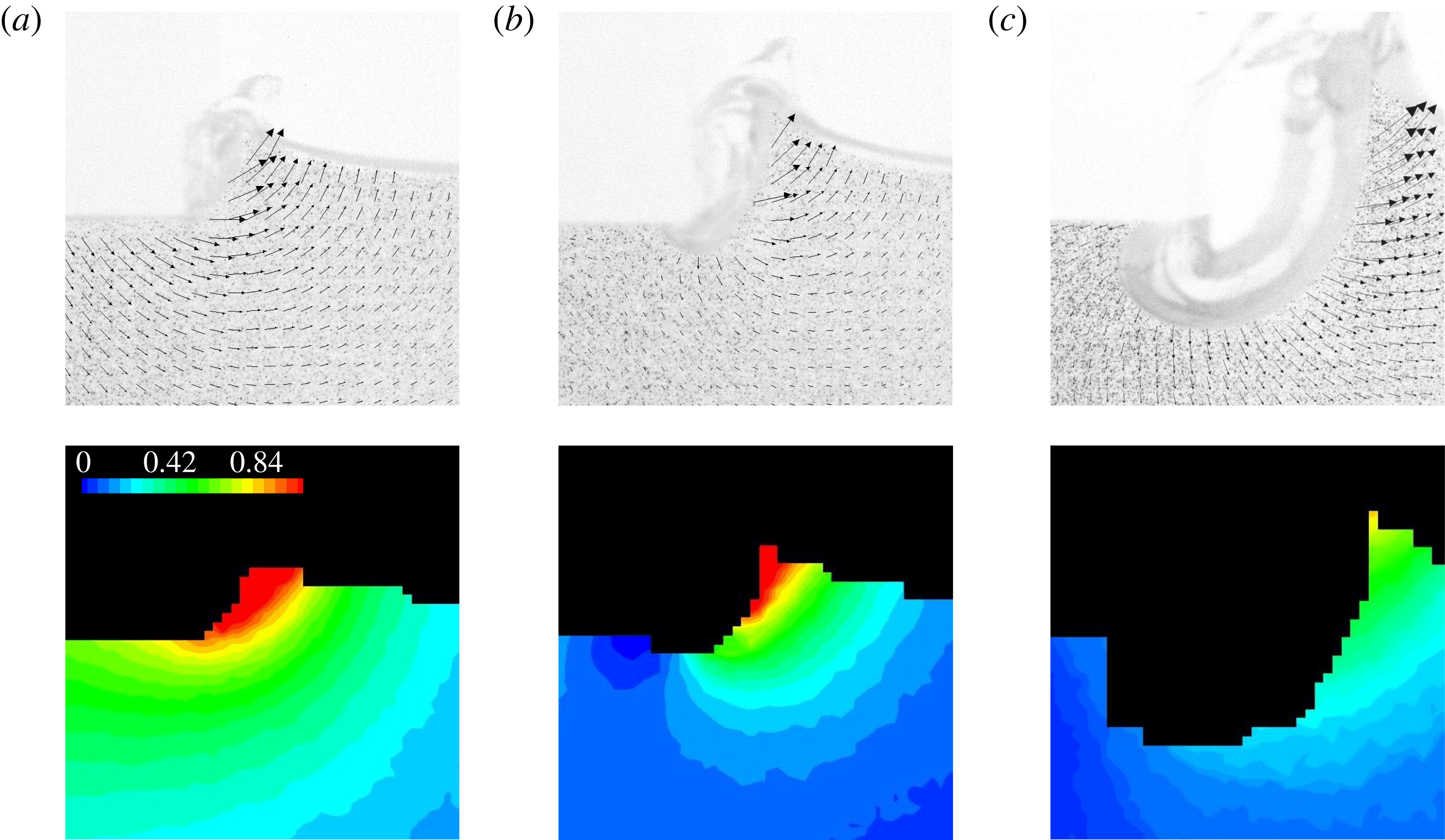
Typical PIV fields around the entrained air pocket growing at the plate edge after the plate penetration has stopped: time increases from panel (a) to panel (c).

6.3 Effects of geometry, viscosity and surface tension
Since the pocket begins to grow immediately after the abrupt deceleration of the impactor, we will label the initial time when the maximum penetration of the plate is achieved by
 $t_{1}$
, see figure 1(d). Herein we are interested in the basic shape and size of the cavity, and therefore we only measure the dimensions at a few locations that define these characteristics throughout the time evolution of the pocket (figure 28):
 $d$
is the maximum depth of the pocket,
 $l^{\prime }$
the extent to which the pocket has penetrated beneath the plate and
 $L$
the approximate width of the pocket. We can then define a pocket aspect ratio as
 $AR=L/d$
. The pocket will grow to a maximum size (characterized by a maximum depth
 $d_{max}$
) in a time
 $t_{cav}$
since the plate stop instant
 $t_{1}$
. Other maximum values (e.g.
 $l_{max}^{\prime }$
and
 $AR_{max}$
) will be taken at
 $t_{cav}$
as well. To better visualize the detailed growth of the air pocket up to the maximum size, the traced pocket edge for four representative impact events is shown in figure 31. Wettability is certainly involved in air pocketing phenomena as is seen from this figure: while for water the contact line is moving appreciably, for high concentration glycerin solutions it is pinned at the plate edge; in the latter case the apparent contact angle varies with time. After reaching the maximum depth the pocket starts to collapse receding from beneath the plate. Collapse of the pocket appears to coincide with the fall of the ejecta from its maximum elevation above the free surface. Notably, the time over which the pocket forms and collapses is nearly an order of magnitude greater than the time for the complete retraction of the trapped air layer beneath the plate, see § 5.
Traced profiles of the air pockets formed near the plate edge after abrupt deceleration of the impactor plate for four liquids – water and glycerol–water mixtures – are presented. In all cases a
 $w=20~\text{mm}$
plate was used with a
 $V_{0}=0.6~\text{m}~\text{s}^{-1}$
impact velocity (corresponding to
 $We\simeq 100$
) and impact depth
 $h=1~\text{mm}$
. The contour ‘water (
 $25.0~\text{ms}$
)’ in (b–d) is given for comparison against the maximum pocket contour in water (a).

From figure 31 we can extract the functional dependence
 $d(t,\unicode[STIX]{x1D707})$
to test the power-law scaling
 $d\sim t^{\unicode[STIX]{x1D6FC}}\,\unicode[STIX]{x1D707}^{\unicode[STIX]{x1D6FD}}$
. As can be gleaned from figure 32(a), the pocket depth scales with time as
 $d\sim t^{\unicode[STIX]{x1D6FD}}$
,
 $\unicode[STIX]{x1D6FD}=0.67-1$
(with the exception of the data for
 $1000~\text{mPa}~\text{s}$
), but the dependence on viscosity is weaker than power law, as per figure 32(b). The data for
 $d_{max}$
were extracted from
 $d(t_{cav})$
curves for a variety of impact conditions (i.e. plate size, impact speed and liquid viscosity) and are presented in figure 33. We can see that the maximum pocket depth increases with impact speed, increases moderately with plate width
 $w$
and decreases with increasing liquid viscosity. Just to guide the eye, region (i) contains most data points for
 $\unicode[STIX]{x1D707}=1{-}100~\text{mPa}~\text{s}$
, while regions (ii) and (iii) contain the majority of data points for
 $\unicode[STIX]{x1D707}=500~\text{mPa}~\text{s}$
and
 $\unicode[STIX]{x1D707}=1000~\text{mPa}~\text{s}$
, respectively.
Log–log plots to test
 $d(t,\unicode[STIX]{x1D707})$
dependence: plot of
 $\log d$
versus
 $\log t$
for four viscosities (a) shows that with the exception of the
 $1000~\text{mPa}~\text{s}$
data (which could be due to a drastic change in the wetting properties),
 $d$
scales with time approximately as
 $d\sim t^{\unicode[STIX]{x1D6FD}}$
with values of the exponent between
 $\unicode[STIX]{x1D6FD}=0.67$
(dotted) and
 $\unicode[STIX]{x1D6FD}=1$
(dashed line); plot of
 $\log d$
versus
 $\log \unicode[STIX]{x1D707}$
for five times (b) shows that the dependence on the viscosity is weaker than power law.
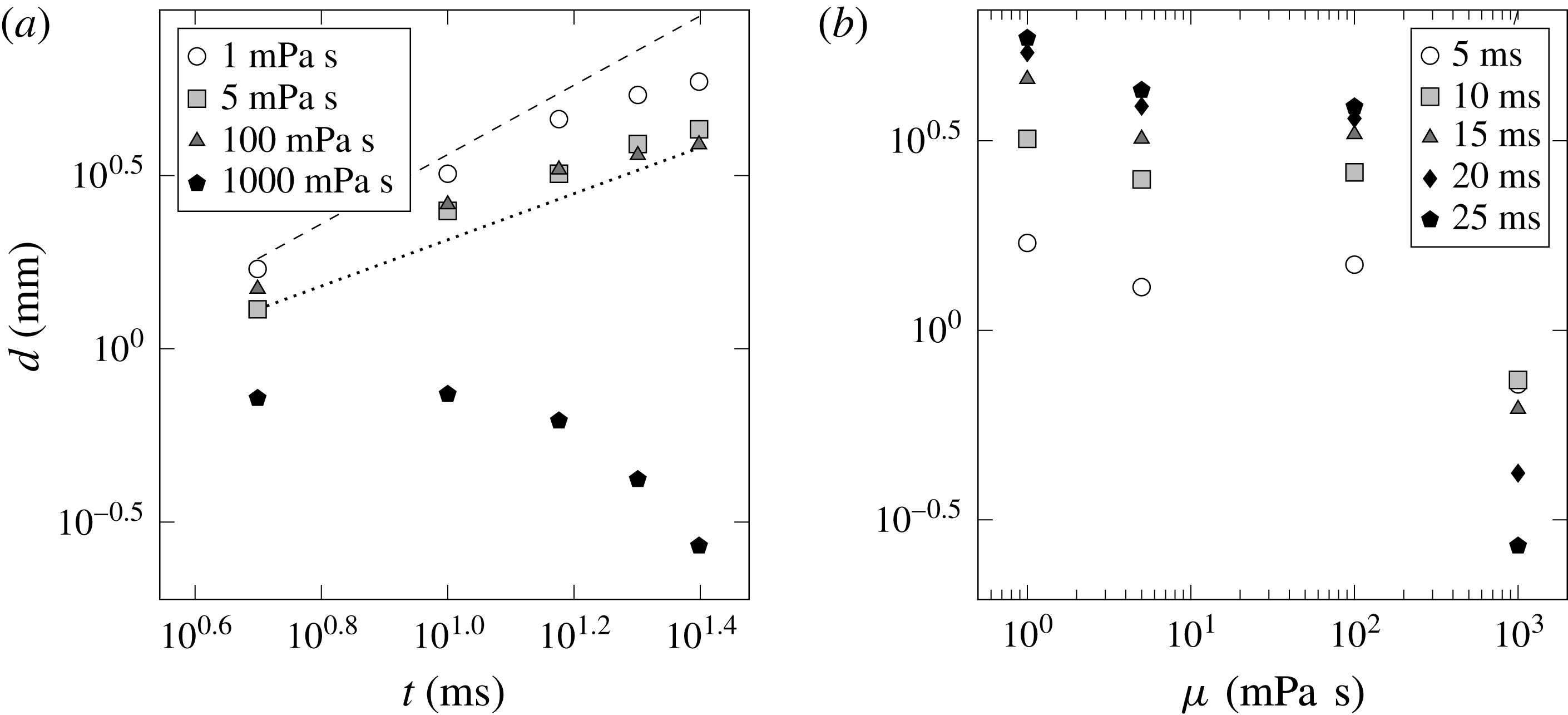
Dimensional plots of
 $d_{max}$
varying with
 $V_{0}$
and
 $h=1~\text{mm}$
. (a) All data for various
 $w$
,
 $\unicode[STIX]{x1D707}$
and
 $\unicode[STIX]{x1D70E}$
. (b) The trend for fixed liquid viscosity (
 $1~\text{mPa}~\text{s}$
) but varying plate size
 $w$
, where
 $w=5~\text{mm}$
(white),
 $10~\text{mm}$
(grey) and
 $25~\text{mm}$
(black). (c) By holding the plate dimension fixed (
 $w=5~\text{mm}$
), we can observe the effect of changing liquid viscosity over the range
 $\unicode[STIX]{x1D707}=1-1000~\text{mPa}~\text{s}$
. Two data sets are provided for
 $\unicode[STIX]{x1D707}=1~\text{mPa}~\text{s}$
, water (circles) and ethanol (triangles). Region (i) contains most data points for
 $\unicode[STIX]{x1D707}=1-100~\text{mPa}~\text{s}$
, while regions (ii) and (iii) contain the majority of data points for
 $\unicode[STIX]{x1D707}=500~\text{mPa}~\text{s}$
and
 $\unicode[STIX]{x1D707}=1000~\text{mPa}~\text{s}$
, respectively. (d) Effect of surface tension variation holding plate width
 $w=5~\text{mm}$
and liquid viscosity fixed.
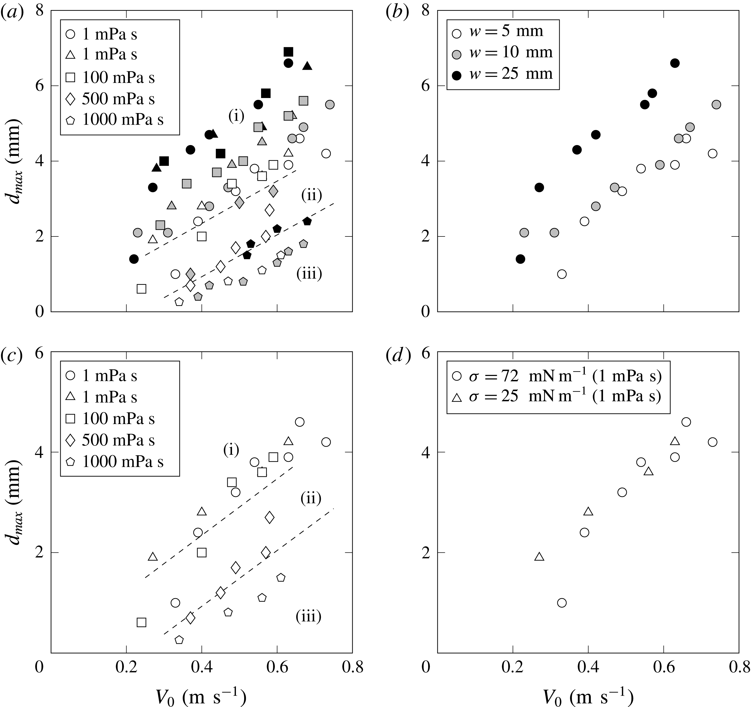
We can also consider the maximum penetration depth of the air pocket beneath the plate edge
 $l_{max}^{\prime }$
compared to the maximum pocket depth
 $d_{max}$
, which is reported in dimensional form in figure 34(a). Here we can see that
 $l_{max}^{\prime }$
tends to be less than
 $d_{max}$
(most points fall below the line with a slope of 1). Using the trends from figures 33 and 34(a) it is apparent that both
 $l_{max}^{\prime }$
and
 $d_{max}$
increase with
 $V_{0}$
. The effect of the liquid viscosity also becomes apparent by inspection of figure 33(c). Note that given all the measurements for the most viscous liquid tested (1000 mPa s) performed in the same range of impact speeds as for other liquids, both
 $d_{max}$
and
 $l_{max}^{\prime }$
are substantially smaller than the values for the less viscous liquids, i.e. increasing viscosity inhibits the growth of the air cavity. While LeGoff et al. (Reference LeGoff, Quere and Clanet2013) found in the experiments on a cavity formation in the impact of a solid spherical projectile that a dramatic increase in the liquid viscosity produced cavities that were wider and shallower than their low viscosity counterparts, we observe drastic changes in the cavity shape and size only for largest liquid viscosity
 $\unicode[STIX]{x1D707}=1000~\text{mPa}~\text{s}$
, as per figure 31(d), with little difference in the qualitative shapes of the cavities in the range
 $1\leqslant \unicode[STIX]{x1D707}\leqslant 100~\text{mPa}~\text{s}$
.
(a) Comparison of
 $l_{max}^{\prime }$
to
 $d_{max}$
suggesting similarity in magnitude. The solid line has a slope of 1. Symbols and shading are consistent with those detailed in figure 33. (b) A similar comparison of
 $L_{max}$
to
 $d_{max}$
, where the solid line now has a slope of 2, reinforces the observation that the maximum aspect ratio
 $AR_{max}$
is
 $\simeq 2$
. Inset shows
 $AR_{max}$
averaged over plate sizes
 $w$
for each fluid as a function of the Morton number.

Comparison of the model (6.3) with the experimental data. (a) Increase of
 $d_{max}/w$
with
 $V_{0}/w$
for all liquids and plate sizes tested. Symbol markers are described in figure 33. The solid line is that of equation (6.3), with a slope of
 $2/3$
on this log–log plot. (b) Effect of impact plate penetration distance
 $h$
on the size of the maximum depth of the air cavity. Here, only data for
 $w=10~\text{mm}$
are plotted, so we can better visualize the discrepancy between the model and the data. The solid line is based on equation (6.3). Inset shows variation in
 $d_{max}$
with fixed depths of impact
 $h$
. These measurements are for water only.
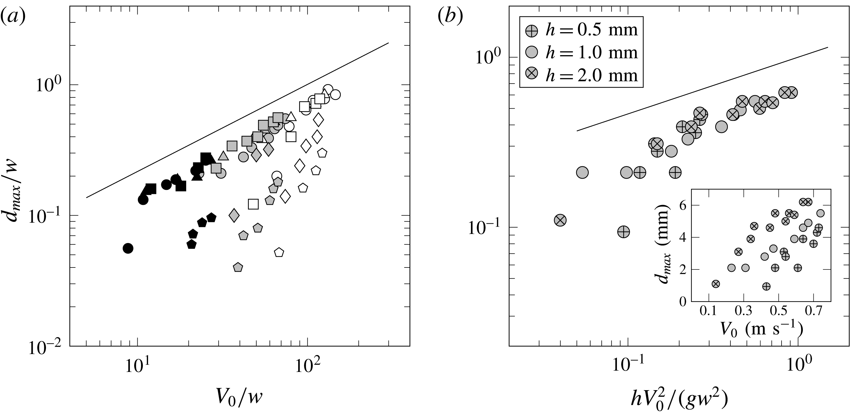
By changing the depth of the plate penetration
 $h$
we can notice its effect on the air pocket size from the inset in figure 35(b). To demonstrate the functional dependence, we measure
 $d_{max}$
for a range of impact speeds and for three different impact depths. Maximum pocket depth is found to increase with
 $h$
as observed in the inset of figure 35(b). Despite the changes in the air pocket size with liquid viscosity, the aspect ratio
 $AR_{max}$
remains largely unaffected, see inset in figure 34(b). This is also evident from figure 34(b), where the measurements of
 $L_{max}$
and
 $d_{max}$
fall along a line with slope 2.
6.4 Simple model and discussion
The natural question to ask is what is responsible for the formation of the entrained air pocket? As opposed to the deep cavities that form following the complete penetration of solid objects into liquids (Richardson Reference Richardson1948; Glasheen & McMahon Reference Glasheen and McMahon1996; Lee et al.
Reference Lee, Longoria and Wilson1997; Leng Reference Leng2001; Bergmann et al.
Reference Bergmann, van der Meer, Gekle, van der Bos and Lohse2009; LeGoff et al.
Reference LeGoff, Quere and Clanet2013), the air pockets produced in our experiments are initiated by the abrupt deceleration of the plate, which is similar to the phenomena in the water exit problem of accelerated lifting of immersed plates from quiescent water, cf. Ostapenko & Kovyrkina (Reference Ostapenko and Kovyrkina2017) and references therein. On the other hand, they also share features similar to transient impact cavities and splashes produced by droplets of liquid falling into deep pools of the same liquid. Although these splash phenomena are quite complex, the observed cavities are nearly hemispherical. Both Pumphrey & Elmore (Reference Pumphrey and Elmore1990) and Leng (Reference Leng2001) found that the maximum cavity depth could be predicted reasonably well using a model based on equating the kinetic energy of the falling drop to the gravitational potential energy of the cavity (while neglecting surface energy of the crater and the potential energy of the crown and ‘wave swell’) leading to
 $R_{max}/d\propto Fr^{1/4}$
. Here
 $R_{max}$
is the maximum depth of the hemispherical crater,
 $d$
the diameter of the splashing droplet and
 $Fr=V_{0}^{2}/(g\,d)$
. Despite neglecting energy losses due to viscous dissipation, reasonable agreement was found by the above authors in both the magnitude and scaling trends, though this model fails to predict the size of (smaller) cavities for viscous liquids (Leng Reference Leng2001).
It is worth highlighting the differences between these liquid drop–liquid pool impact experiments and our own, and then proceeding with the development of a predictive model for the air pocket size. The air pockets that we observed form well after the impact of a flat plate with the liquid surface, and only when the plate has penetrated to a set depth
 $h$
and abruptly stopped. Because of the mechanical stop, the plate has zero kinetic energy at the start of the air pocket evolution. Furthermore, the flow field rapidly reverses immediately after the abrupt deceleration – from the PIV measurements in figure 29(b) it appears as though the velocity of the fluid, except for the ejecta, is negligible at the start of cavity formation. But there is still considerable kinetic energy associated with the ejecta, formed prior to the development of the pocket.
Our method for determining a scaling for the maximum cavity depth invokes a balance between the kinetic energy of the ejected liquid and the potential gravitational and surface energies of the air pocket. Both of the latter energies will be evaluated when the cavity has reached its maximum depth, and the ejected liquid attained its apex and therefore has negligible velocity. Given such an energy balance neglecting dissipation, the predicted scaling is expected to apply only to the low viscosity liquids.
Considering half of the plate in view of symmetry, the following are the estimates for the various energy terms per unit length of the plate (dropping all numerical coefficients):
(i) the surface energy of the pocket – a cylinder of radius
 $d_{max}$
, based on the fact that the aspect ratio
$AR=O(1)$
, in agreement with figure 34(b) – per unit length is defined as
$SE_{cav}\sim \unicode[STIX]{x1D70E}\,d_{max}$
;
(ii) the kinetic energy of the ejected liquid defined as
$KE_{ej}\sim \unicode[STIX]{x1D70C}\,w\,h\,V_{0}^{2}$
, which is based on a simple estimate: the mass displaced by the impact plate during the penetration stage
$\unicode[STIX]{x1D70C}\,w\,h$
has been imparted with a velocity of the order of
$V_{0}$
;(iii) the gravitational potential energy of the cavity
$PE_{cav}\sim \unicode[STIX]{x1D70C}\,d_{max}^{2}\,g\,d_{max}$
, where, similar to Pumphrey & Elmore (Reference Pumphrey and Elmore1990), we used
$d_{max}$
to characterize the difference in elevation between the undisturbed free surface of the liquid pool and the centre of mass
$h+4\,d_{max}/(3\,\unicode[STIX]{x03C0})$
of the cavity, treated as a cylinder shaped pocket formed at a depth
$h\ll d_{max}$
as a result of the plate penetration.





The balance of the energy terms is then
 $$\begin{eqnarray}\unicode[STIX]{x1D70C}whV_{0}^{2}\sim \unicode[STIX]{x1D70C}gd_{max}^{3}+\unicode[STIX]{x1D70E}d_{max}.\end{eqnarray}$$
If we consider a ratio of the gravitational and surface energies,
 $\unicode[STIX]{x1D70C}\,g\,d_{max}^{2}/\unicode[STIX]{x1D70E}\equiv Bo$
(the Bond number), and use representative values from our experiments, e.g.
 $d_{max}\sim 3~\text{mm}$
, we find that
 $Bo\gg 1$
. So we can further simplify (6.1) by neglecting the effects of surface energy, which is consistent with the observations in figure 33(d) that variation in surface tension does not affect the entrained air pocket evolution. Therefore, equating the kinetic energy of the ejected mass and the potential energy of the pocket furnishes
 $$\begin{eqnarray}\unicode[STIX]{x1D70C}\,w\,h\,V_{0}^{2}\sim \unicode[STIX]{x1D70C}\,g\,d_{max}^{3}\rightarrow d_{max}/w\sim Fr^{1/3}(h/w)^{1/3},\end{eqnarray}$$
where now
 $Fr=V_{0}^{2}/(g\,w)$
. Equation (6.2) can also be written as
 $$\begin{eqnarray}d_{max}/w\sim (V_{0}/w)^{2/3}(h/g)^{1/3},\end{eqnarray}$$
which can be arrived at via dimensional analysis. The plot in figure 35(a) shows the dependence of
 $d_{max}/w$
on
 $V_{0}/w$
for a fixed impact depth of
 $h=1~\text{mm}$
and a variety of plate widths. It is apparent that the data for liquids with viscosity
 $1\leqslant \unicode[STIX]{x1D707}\leqslant 100~\text{mPa}~\text{s}$
tend to collapse together, while beyond this viscosity range separate trends emerge, e.g. notice the data for
 $\unicode[STIX]{x1D707}=500~\text{mPa}~\text{s}$
and
 $\unicode[STIX]{x1D707}=1000~\text{mPa}~\text{s}$
. This is expected: as the liquid viscosity increases, friction forces become significant preventing the inertia of the liquid from forming the deep pockets predicted by the inviscid estimate (6.2), see figure 31(d).
We can also test the scaling of
 $d_{max}$
with the impact plate penetration depth
 $h$
by re-plotting the raw data in the inset of figure 35(b) according to the scaling (6.3). This is shown in figure 35(b), where the solid line again representing the model lies above the measurements, which results from the energy unaccounted for in the balance of (6.2) due to viscous dissipation and the formation of air–liquid interface. Also, since the model underpredicts
 $d_{max}$
, as follows from figure 35, a possible effect is that of added mass: the larger the penetration depth
 $h$
, the larger the displaced liquid mass and hence, in addition to the negative gauge pressure mechanism, there is a simple effect of larger kinetic energy of downward moving fluid as evidenced by the velocity field in figure 30(b,c) and the obvious increase of
 $d_{max}$
with
 $h$
in the inset of figure 35(b). Basically, not all energy goes into
 $KE_{ej}$
, which is why the measured
 $d_{max}$
is lower than predicted by (6.3).
Finally, the energy model (6.3) does not explain figure 32 – one needs to understand the mechanism that controls the time rate at which energy is transferred from left to right in (6.2), apparently largely independent of dissipation in the range of viscosities
 $1{-}100~\text{mPa}~\text{s}$
. Since the hammering pressure
 $\unicode[STIX]{x0394}p$
drives the added mass of the liquid surrounding the cavity
 $m\sim \unicode[STIX]{x1D70C}\,d^{2}$
per unit length of the plate, Newton’s second law furnishes
 $$\begin{eqnarray}\text{d}(m\,v)/\text{d}t=\unicode[STIX]{x0394}p\,S(d),\end{eqnarray}$$
where
 $v\sim d^{\prime }(t)$
and the area
 $S$
on which the pressure acts is a function of
 $d$
. If we assume
 $\unicode[STIX]{x0394}p=\text{const.}$
and
 $S\sim d$
, then (6.4) gives
 $d\sim t$
, which is the upper bound on the growth observed in figure 32(a). However, the hammering pressure drops with time, e.g. due to viscous dissipation, which explains slightly slower growth of
 $d(t)$
observed experimentally.
7 Conclusions
We have presented a new experimental set-up that, as a result of overcoming the challenges with optical access, enabled us to study two-dimensional flat plate impact on water. Imaging of the flow field and ejecta resulting from impact was accomplished using high-speed photography and PIV. We demonstrated that in view of repeatability of the impact event it is possible to construct a time series of PIV flow fields without recourse to a high frame rate PIV system. The optical access of our set-up allowed us to resolve fine details of the flow field near the plate edge and even inside the ejecta.
PIV analysis of the flow field produced by plate impact shows that significant deviation from the inviscid flow theory exists near the plate edge. Over the range of
 $Re$
and
 $We$
numbers studied here, Yakimov’s scaling for the flow field is not observable simply because the region where
 $\boldsymbol{v}\sim r^{-1/2}$
does not exist and, moreover, the KJ condition proved to be not universally applicable. How velocity vectors depart from the plate edge depends, in particular, on the wetting properties between the plate material and liquid.
Free surface scaling near the edge in the Stokes regime and in the far field proved to conform with the existing theories. Probing the water impact phenomena at even higher
 $Re$
and
 $We$
numbers in the region close, but not right next, to the plate edge, might exhibit the singular
 $\boldsymbol{v}\sim r^{-1/2}$
and thus Yakimov’s scaling for the free surface. Right next to the plate edge, such experiments are expected to give similar results to ours as the same physical effects not accounted in the classical inviscid theory will be present as well. Our experiments also indicate that ejecta surface profiles are approximately self-similar with deviations from self-similar behaviour due to viscosity, surface tension and wetting properties. While the existence of self-similarity is conceptually analogous to the scaling suggested by Yakimov, the spatial scaling significantly deviates from his predictions with the approximate self-similarity exponent dependent on the impact conditions. Effects of viscosity and surface tension on the ejecta formation revealed that increasing the former flattens the ejecta, while decreasing the latter makes the ejecta thinner.
We have also investigated several interesting phenomena associated with the later stages of a flat plate impact that have not been explored in the literature before, specifically retraction of trapped air beneath impact plates and air pocketing at the impact plate edges. The non-monotonic dependence of the volume of trapped air with the impact speed is surmised here to be caused by the compressible flow effects in the unsteady nozzle regime, which are yet to be understood. The mechanism for the rapid initial retraction of the trapped air is a consequence of a negative pressure impulse generated upon the abrupt deceleration of the plate and the subsequent slower retraction can be described with an inertial model. The plate’s abrupt deceleration is also the cause of the air pocketing. The maximum depth of the resulting pocket has been predicted using an energy balance and the time evolution of the growing pocket was explained with the basic force balance, though the complete theoretical understanding including viscous and surface tension effects awaits further investigation.
Among other open questions is the effect of wetting on the angle at which the ejecta departs the plate. While we showed that the KJ condition is not universally applicable, i.e. the departure angle is non-zero and, in fact, a function of time, it would be interesting to understand how the variation of the static contact angle affects the dynamic departing angle, how the latter varies with wettability, and if there is any significant effect on the ejecta evolution. In spirit, such a study would be analogous to that of Duez et al. (Reference Duez, Ybert, Clanet and Bocquet2007), who established a relation between a threshold impact velocity for air entrainment and the wetting contact angle: despite the fact that the contact angle is dictated by microscopic phenomena, the latter have an effect on the macroscopic behaviour of the problem, in particular global splashing characteristics. In the case of water impact phenomena, the presence of a trapped air is analogous to the effect of hydrophobicity and is known to affect the ejecta development (Yakimov Reference Yakimov1973; Ermanyuk & Ohkusu Reference Ermanyuk and Ohkusu2005).
Acknowledgements
This work was partially supported by the National Science Foundation (NSF) CAREER award under grant no. 1054267 and the Natural Sciences and Engineering Research Council of Canada (NSERC) under grant no. 6186. The authors would also like to thank Mr M. Houlahan for the assistance with building the water tank, Mr H. Habibi for the help with accelerometric measurements, and anonymous referees for constructive feedback. R.K. is grateful to Professor V. Pukhnachev who sparked my interest in the water impact phenomena, Professor M. Tulin for encouraging conversations and for donating part of his research library, Professor B. Homsy for commenting on the earlier version of the manuscript and Dr A. Zelnikov for stimulating discussions.
Appendix. Optical access
(a) Front view image of the impact plate sitting just above the free surface of the liquid. The front and back walls are as indicated, and the scale bar represents a distance of
 $10~\text{mm}$
. The purpose of this image is to orient the reader to images and sequences provided in the text. Typically the camera is at a much shallower angle with respect to the liquid surface. (b,c) Sequences of images of a
 $w=10~\text{mm}$
impact plate striking the surface of water with a velocity of
 $V_{0}=0.35~\text{m}~\text{s}^{-1}$
(corresponding to
 $We=17$
). Each image is time stamped after the impact moment. (b) With a wall-to-plate gap of
 $3.5~\text{mm}$
the spacing is shown to obscure visualization of the impact event despite a nearly 2-D flow as evidenced by the regular appearance of the ejecta along the length of the plate, away from the walls. As early as
 $5~\text{ms}$
the flow field near the ejecta is distorted at the bottom corner of the plate. Later, the region of the flow field beneath the plate (highlighted at
 $20~\text{ms}$
) is screened by the air pocketing occurring along the front edge. (c) By reducing the wall-to-plate gap to
 $0.5~\text{mm}$
(less than the capillary length), a remarkable improvement in optical access is gained. We can view into the ejecta at early times, observe the flow field beneath the plate and capture a front view of the trapped air retraction event (highlighted at
 $20~\text{ms}$
).

To house the liquid for all impact experiments, a transparent long rectangular plastic tank, whose width (in the horizontal direction, i.e. between front and back walls) was nearly equal to the length of the impact plate (i.e.
 $\simeq 70~\text{mm}$
), was used. The narrow gaps separating the ends of the plate and front/back walls were made as small as
 $0.01~\text{mm}$
to minimize any significant flow of the displaced air through these sides of the plate: as is easy to estimate, viscosity of air impedes its motion through the gap of size
 $0.01~\text{mm}$
in approximately
 $10^{-2}~\text{ms}$
, i.e. on a much shorter time scale compared to our measurements. Hence, the air is forced to escape only through the long sides of the plate resulting in the two-dimensional (2-D) evolution of the trapped air layer discussed in § 5.3 and illustrated in figure 24. This also allows us to produce a nearly 2-D flow field in the middle section of the tank half-way between the front and back walls where the measurements are taken, so that the results would be directly comparable to existing 2-D theory. Figure 36(a) shows the field of view from a camera (which could be either a high-speed or PIV camera) looking along the length of the plate positioned just above the free surface. The 2-D geometry makes it possible to perform flow visualization inside the ejecta otherwise impracticable with a more traditional experimental set-up using circular disks or other axisymmetric impacting bodies (e.g. spheres, cylinders, cones). The dramatic difference between a circular disk (Peters et al.
Reference Peters, van der Meer and Gordillo2013) and the 2-D plates with small plate–wall gaps is displayed in figure 37: the much improved optical access constitutes a unique feature of our apparatus. Neither such a visualization can be accomplished with 2-D plates that leave too much of a gap between the front and back walls of the tank as highlighted in figure 36(b), which allows the splash to impede optical access into the region near the ejecta formation. The region beneath the impact plate and near the edge is also concealed. By reducing the gap to
 $0.01~\text{mm}$
, we greatly improve optical access to all regions as shown in figure 36(c).
The flow field and surface deformations resulting from impact are obtained using a PIV system (TSI, Inc.). A dual-pulse Nd:YAG laser (Evergreen
 $200~\text{mJ}$
) generates a laser light sheet that illuminates tracer particles beneath the middle of the plate. The time of the first laser pulse can be varied using a trigger-delay unit (BNC model 575) according to a step-rise voltage signal created when the impact plate, connected to a low voltage source, contacts the liquid containing a submerged electrode and a small amount of sodium chloride (NaCl),
 $\simeq 5~\text{g}~\text{L}^{-1}$
, added in order to make it conductive while the surface tension being affected by not more than one per cent (Jones & Ray Reference Jones and Ray1941). By adjusting the delay of the first laser pulse while holding all other variables (e.g. impact velocity), a time history of the flow field beneath the impact plate and of the surface shape can be built. Repeatability of PIV snapshots with the same time delay was verified and even in the extreme case when the time delay since the moment of impact is
 $50~\text{ms}$
, i.e. much later compared to the time scales of our experiments, the error associated with two PIV snapshots is only
 $5.7\,\%$
. For PIV snapshots taken for much shorter times
 $0{-}2~\text{ms}$
after impact, such as in most of our experiments, is even smaller.
A comparison of optical access for (a) a circular disk-shaped impact plate (
 $V_{0}=0.6~\text{m}~\text{s}^{-1}$
,
 $r=10~\text{mm}$
,
 $h=1~\text{mm}$
,
 $t=\text{5 ms}$
) and (b) a rectangular impact plate (
 $V_{0}=0.2~\text{m}~\text{s}^{-1}$
,
 $w=10~\text{mm}$
,
 $h=1~\text{mm}$
,
 $t=5~\text{ms}$
) spanning the tank width. Both are filmed using a high-speed camera. The axisymmetric impact plate produces an axisymmetric ejecta. However, the rectangular plate spanning the tank produces a 2-D flow field, thus providing optical access into the ejecta and splash. The scale bar represents
 $10~\text{mm}$
.

With minor modifications to the system, the PIV camera can be replaced with a high-speed digital camera (Phantom v5.2) and back lighting is provided by an LED source (IDT, Inc.) to produce bright-field imaging. Also, the mirror used to direct the PIV laser sheet can be employed to image the details of the impact event from below.