1 Introduction
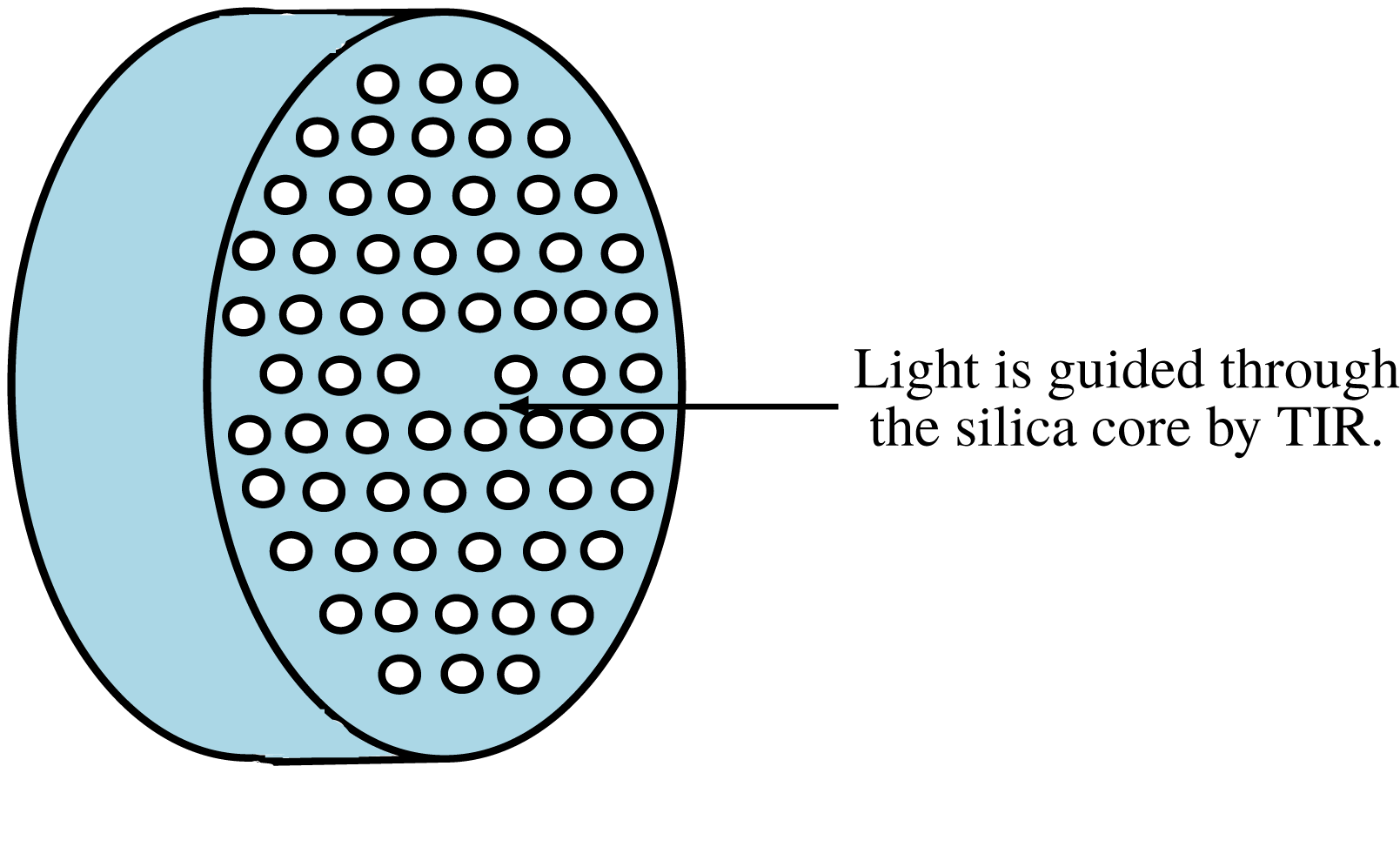
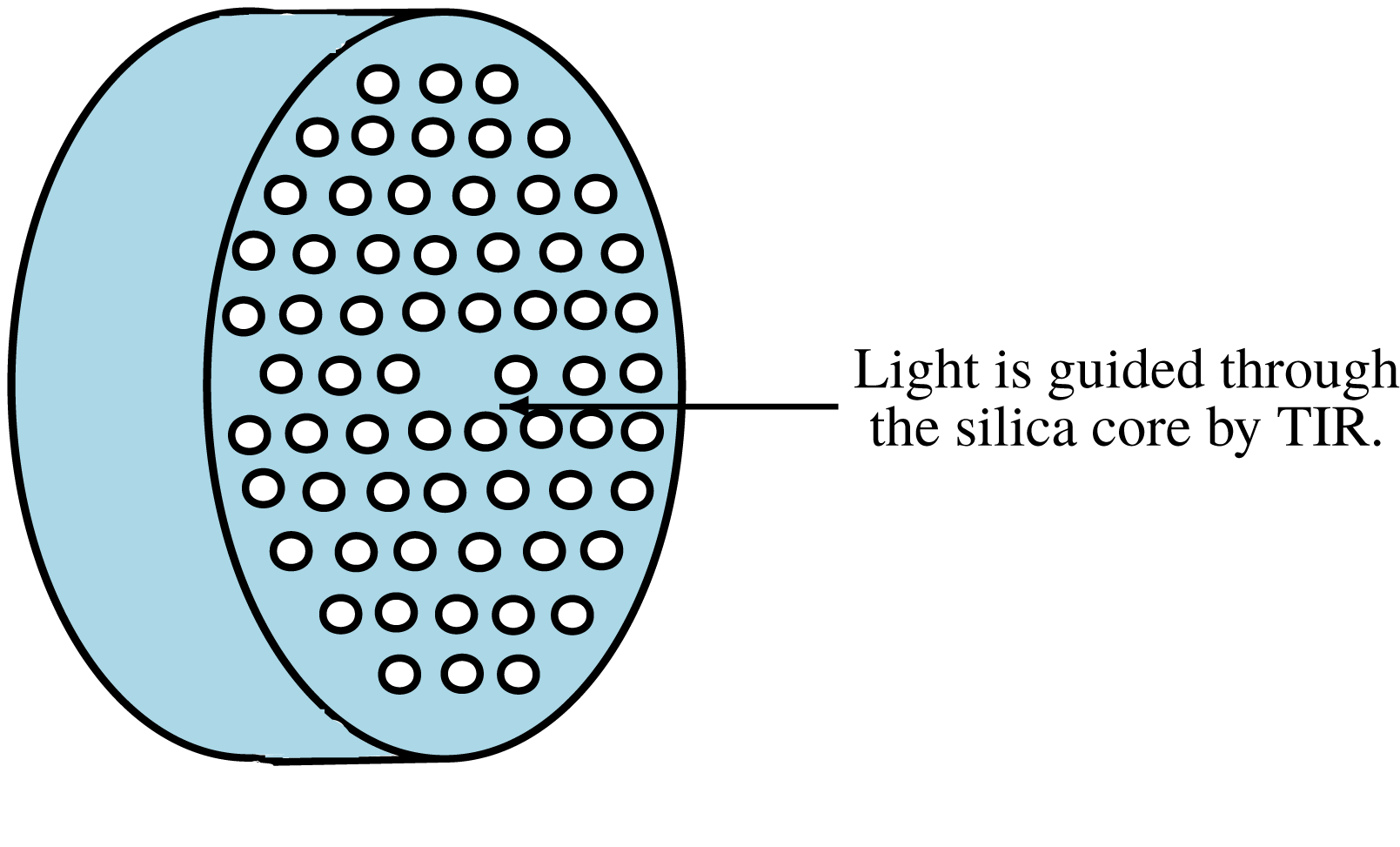
A conventional optical fibre is typically made from two different layers of glass: a doped inner core and an outer cladding of pure silica (Senior & Jamro Reference Senior and Jamro2009). Light travels along the fibre by the process of total internal reflection at the interface between the core and the cladding, which have different refractive indices. There is currently great interest in the fabrication of a relatively new type of microstructured optical fibre (MOF), made of a single material, with the cladding region containing an array of air holes that run along the entire fibre length, as illustrated by the example in figure 1 (Wynne Reference Wynne2006). These holes provide an effective difference in the refractive index, and thus light passing through the core is guided by total internal reflection in a similar manner to a conventional optical fibre. The air channels can be arranged in a multitude of patterns, and it is due to this flexibility that MOFs can be produced with adaptable optical properties (see, for example, Birks, Knight & Russell Reference Birks, Knight and Russell1997; Monro et al. Reference Monro, Richardson, Broderick and Bennett1999; Ranka, Windeler & Stentz Reference Ranka, Windeler and Stentz2000).
Schematic diagram of a segment of a microstructured optical fibre; air holes are arranged in a hexagonal lattice in the cladding region (Hansen et al. Reference Hansen, Broeng, Skovgaard, Folkenberg, Nielsen, Petersson, Hansen, Jakobsen, Simonsen and Limpert2005), running along the entire length of the fibre.
A MOF is constructed by heating a macroscopic silica preform (typically a few centimetres in diameter) and then drawing it down into a fibre, typically
 $125~\unicode[STIX]{x03BC}\text{m}$
in diameter, at a speed of
 $10{-}50~\text{m}~\text{min}^{-1}$
(Fitt et al.
Reference Fitt, Furusawa, Monro, Please and Richardson2002). To achieve the desired optical properties, the MOF must be constructed with a precise air-channel configuration. The fluid flow that arises during the manufacturing and drawing processes can lead to distortions in the preform that render the fibre useless even if one specifies the initial arrangement of the air channels. Unwanted side effects such as changes in the shape, size or location of the air holes or even complete closure of the air holes, have been experimentally observed (Ebendorff-Heidepriem & Monro Reference Ebendorff-Heidepriem and Monro2007; Ebendorff-Heidepriem, Moore & Monro Reference Ebendorff-Heidepriem, Moore and Monro2008). A mathematical model enabling the manufacturing process to be properly understood, controlled and optimized would resolve the current costly and time-consuming trial-and-error nature of the largely experimental fabrication process.
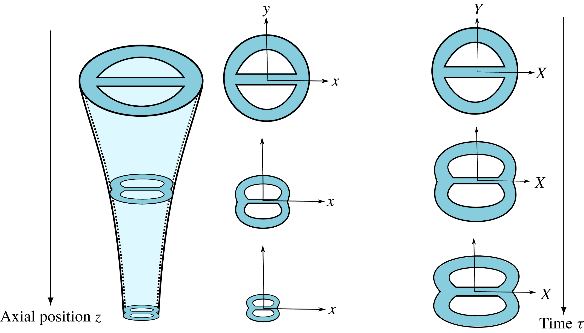
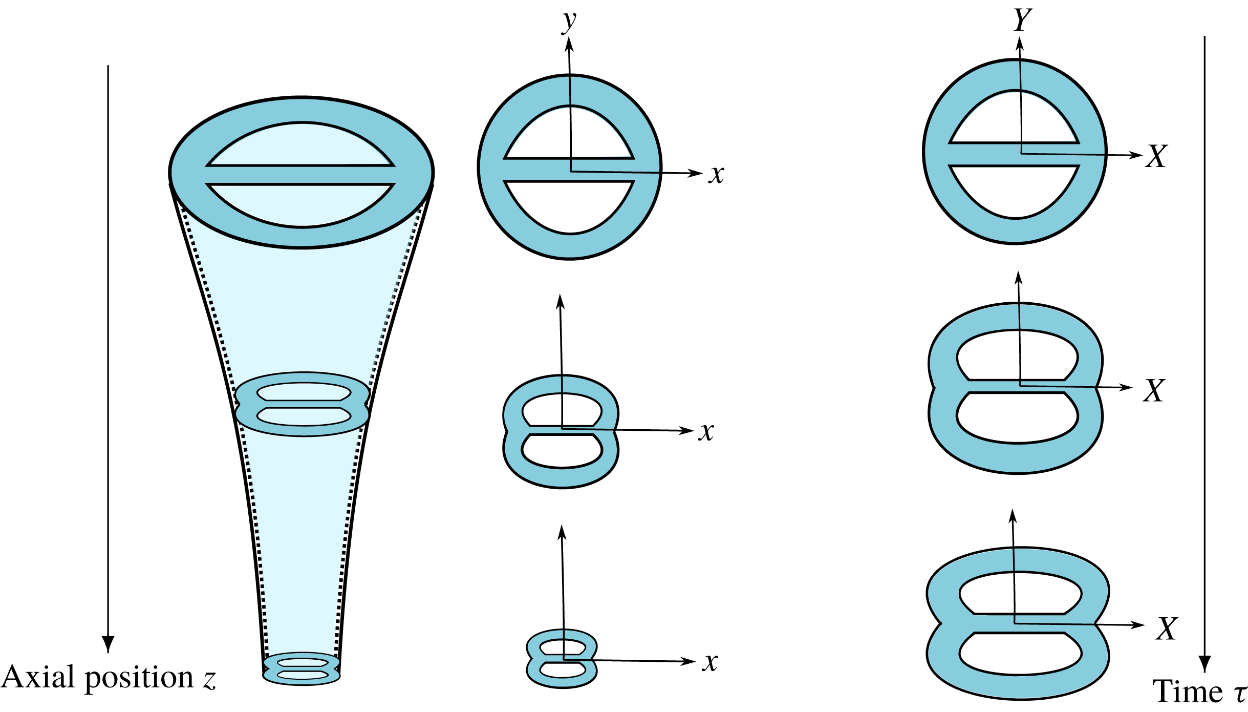
Predicting the full evolution of a MOF during the drawing process is a formidable challenge, but fortunately one can exploit various geometrical features to simplify the problem. If one assumes that the fibre cross-section is slowly varying in the axial direction then, in a suitable Lagrangian frame of reference, the shape evolution of the cross-section is reduced to a classical two-dimensional Stokes-flow free-boundary problem. (This asymptotic decoupling can also give a useful approximation to the real behaviour even when the axial variations are not so slow.) The transverse-flow problem is coupled with a one-dimensional axial-stretching problem, determining the size of the cross-section as a function of axial distance. The approach is illustrated schematically in figure 4, and has been used successfully in, for example, Dewynne, Ockendon & Wilmott (Reference Dewynne, Ockendon and Wilmott1989), Dewynne, Howell & Wilmott (Reference Dewynne, Howell and Wilmott1994) and Cummings & Howell (Reference Cummings and Howell1999) to describe the evolution of a fibre with arbitrary simply-connected cross-section. In Griffiths & Howell (Reference Griffiths and Howell2007, Reference Griffiths and Howell2008) the same insight is used to model the cross-sectional shape of a slender thin-walled viscous tube with uniform thickness at each cross-section, subject to deformations due to both axial stretching and surface tension. Stokes et al. (Reference Stokes, Buchak, Crowdy and Ebendorff-Heidepriem2014) build on the same ideas to present a general mathematical framework to model the pulling of slender optical fibres whose cross-section can have any geometry, including multiple holes.
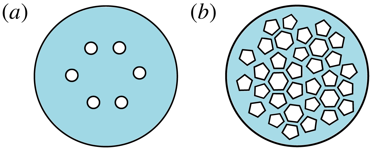
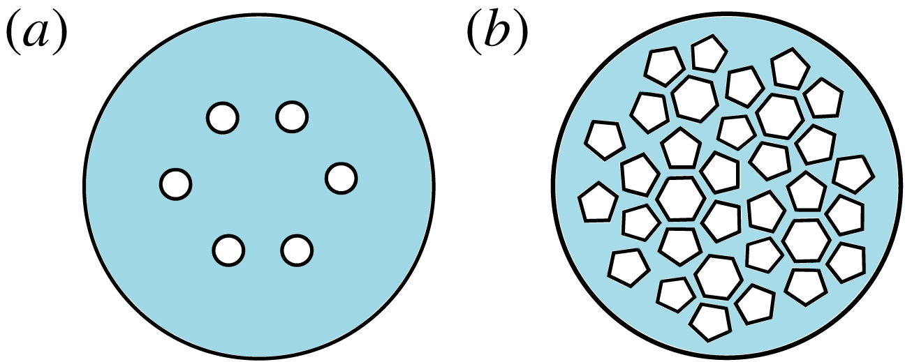
Schematic diagrams of the cross-sections of MOFs with air channels that are (a) well spaced and (b) closely spaced.
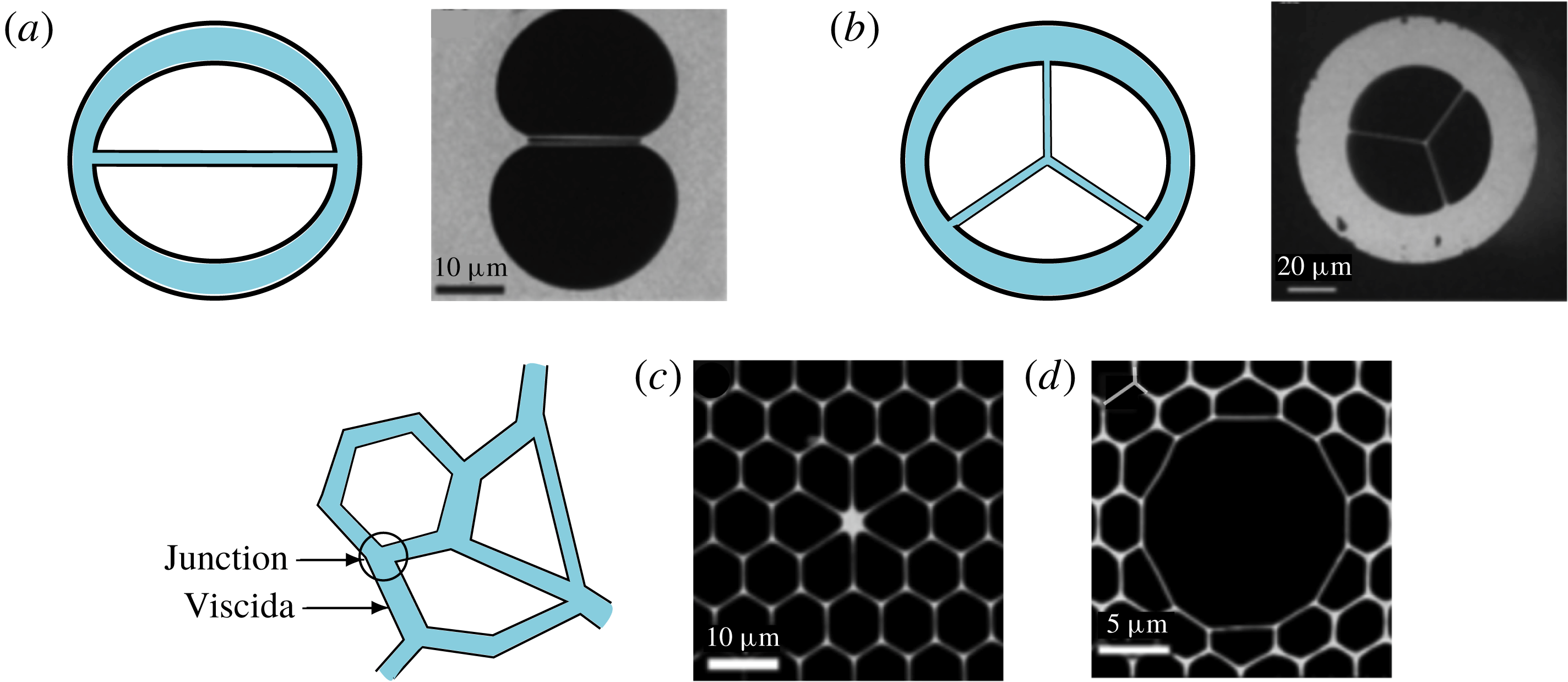
High-quality scanning electron microscope (SEM) images of the cross-section of (a) germanate double-nanoweb fibre, (b) germanate suspended-core fibre, (c) lead-silicate multi-component bandgap fibre and (d) lead-silicate highly nonlinear photonic crystal fibre; (a–c) have a solid core and (d) has a hollow core. All of these are examples of soft glass photonic crystal fibres made at the Max Planck Institute for the Science of Light (Russell Reference Russell2019). The blue figures are the equivalent schematic diagrams.
Having exploited the slenderness in the axial direction, it remains to solve the resulting two-dimensional Stokes-flow problem. Motivated by the fabrication process of MOFs, Buchak & Crowdy (Reference Buchak and Crowdy2016) present a numerical scheme to solve a two-dimensional Stokes-flow problem with multiple interacting free boundaries whose evolution is driven by surface tension. Similarly, a model for fibre evolution based upon complex-variable methods is presented in Tronnolone (Reference Tronnolone2016), where the focus is on the extrusion stage of the fabrication process. Modelling of fibre drawing with deformation of channels due to stretching, surface tension and pressurization has been treated in Chen et al. (Reference Chen, Stokes, Buchak, Crowdy and Ebendorff-Heidepriem2015). Finally, the model described in Buchak et al. (Reference Buchak, Crowdy, Stokes and Ebendorff-Heidepriem2015) uses two asymptotic approximations: that the fibre is slender and that the cross-section of the fibre is a circular disc with well-separated elliptical channels that are sufficiently far from the outer boundary. This approach regularizes the ill-posed inverse problem of the fabrication of MOFs.
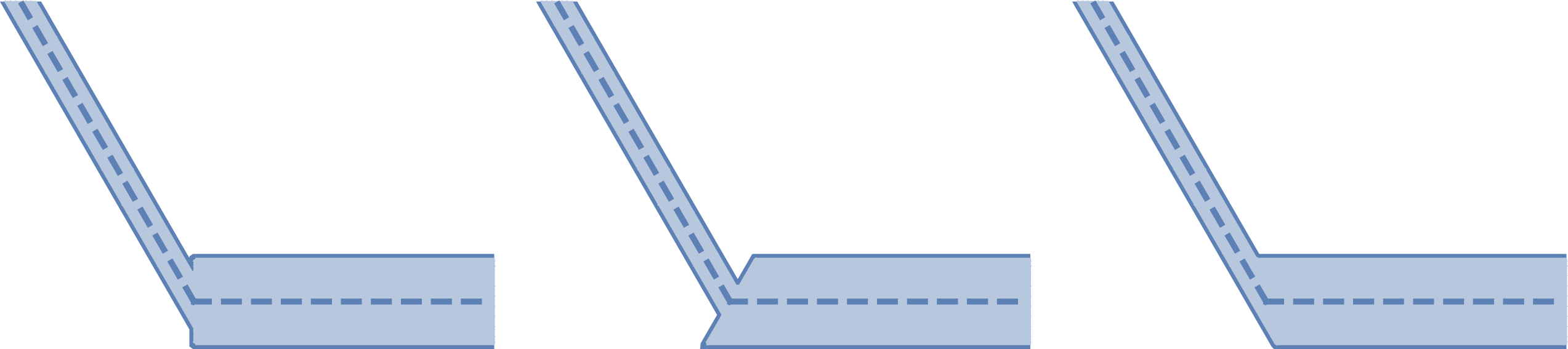
The approximate model derived by Buchak et al. (Reference Buchak, Crowdy, Stokes and Ebendorff-Heidepriem2015) is valid when the holes are well spaced (see figure 2 a). However, many MOFs lie at the opposite limit, in which the holes are very close together (see figure 2 b); typical real examples are shown in figure 3. Our focus in this paper is on such geometries, where it is no longer appropriate to model individual holes that are weakly coupled through a bulk Stokes flow. Instead, one can exploit the geometrical assumption that the holes are closely spaced, so that the cross-section can be thought of as being composed of a network of very thin sheets of glass, or viscidas (Buckmaster, Nachman & Ting Reference Buckmaster, Nachman and Ting1975; Buckmaster & Nachman Reference Buckmaster and Nachman1978), which are connected together at junctions (see schematics in figure 3). In this paper we develop such a theory by extending the model for a single viscida derived by Griffiths (Reference Griffiths2007) and Griffiths & Howell (Reference Griffiths and Howell2007, Reference Griffiths and Howell2008) to describe the behaviour at a junction where two or more viscidas meet and to allow for variations in thickness. The resulting coupled model is used to tackle a series of canonical problems that form the building blocks of the full problem of the evolution of a MOF cross-section with closely spaced holes.
Two-dimensional model to describe the shape evolution of the cross-section of a microstructured optical fibre.
We begin in § 2 by recapping the governing equations for a single surface-tension-driven viscida. In § 3 we study the behaviour at a junction where several viscidas meet. The case of two connected viscidas is modelled as a smoothed corner in a single viscida, and we show that a well-defined evolution law is obtained in the limit as the smoothing parameter tends to zero. This angle-evolution law is then generalized to an arbitrary number of interacting viscidas by performing a local moment balance. In § 4 we combine the ideas from §§ 2 and 3 to derive a coupled model for a system of viscidas connected at junctions. We work in detail through two examples containing two and three viscidas, respectively, before presenting a general theory for an arbitrary viscida network which, in theory, allows us to capture the behaviour of complex MOF cross-sections such as those depicted in figure 3. We use this theory in an example of a six-viscida configuration. In § 5, we extend the analysis to include variations in thickness along and between the viscidas. This apparently innocuous generalization exposes an interesting degeneracy in the modelling of a junction between viscidas of differing thicknesses. Finally, in § 6, we discuss our results and draw our conclusions.
2 Governing equations for a viscida
Consider a thin two-dimensional sheet of viscous liquid which is invariant in the
 $z$
-direction, whose thickness is given by
 $h(s,t)$
and whose centreline in the
 $(x,y)$
-plane makes an angle
 $\unicode[STIX]{x1D703}(s,t)$
with the
 $x$
-axis, where
 $s$
is arc-length and
 $t$
is time. Griffiths & Howell (Reference Griffiths and Howell2007) derived a model for the evolution of such a viscida by performing an asymptotic analysis in the limit where the aspect ratio
 $\unicode[STIX]{x1D716}$
of typical thickness
 $\overline{h}$
to typical length
 $\overline{L}$
tends to zero. Here we present the resulting leading-order dimensionless governing equations, in which lengths are made dimensionless with
 $\overline{L}$
, thickness with
 $\overline{h}=\unicode[STIX]{x1D716}\overline{L}$
and time with
 $\overline{h}\unicode[STIX]{x1D707}/\unicode[STIX]{x1D6FE}$
, where
 $\unicode[STIX]{x1D707}$
and
 $\unicode[STIX]{x1D6FE}$
denote the constant viscosity and surface tension, respectively.
A balance of forces and moments at each point along the viscida leads to the identity
 $$\begin{eqnarray}\frac{\unicode[STIX]{x2202}M}{\unicode[STIX]{x2202}s}=-A(t)\sin \unicode[STIX]{x1D703}-B(t)\cos \unicode[STIX]{x1D703},\end{eqnarray}$$
where
 $M(s,t)$
is the bending moment, while
 $A(t)$
and
 $B(t)$
are the spatially uniform net tensions in the
 $x$
- and
 $y$
-directions. These two functions must also be determined as part of the solution; the signs are chosen simply for convenience. The leading-order constitutive relation for the bending moment is
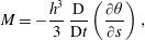 $$\begin{eqnarray}M=-\frac{h^{3}}{3}\,\frac{\text{D}}{\text{D}t}\left(\frac{\unicode[STIX]{x2202}\unicode[STIX]{x1D703}}{\unicode[STIX]{x2202}s}\right),\end{eqnarray}$$
where
 $\text{D}/\text{D}t$
is the material time derivative following a particular section through the viscida. Finally, an evolution equation for the thickness of the viscida arises from a balance between the viscous tension and the surface tension. The viscous tension in a two-dimensional thin viscous sheet is given (in dimensional variables) by
 $-4\unicode[STIX]{x1D707}\text{D}h/\text{D}t$
(Griffiths & Howell Reference Griffiths and Howell2007), while the net contribution of surface tension at the two free surfaces is
 $2\unicode[STIX]{x1D6FE}$
. A net tangential force balance thus leads to the dimensionless equation
 $$\begin{eqnarray}\frac{\text{D}h}{\text{D}t}=\frac{1}{2},\end{eqnarray}$$
which describes a constant rate of thickening of each material section under the action of surface tension.
In principle, equations (2.1)–(2.3) provide a closed system for
 $M(s,t)$
,
 $h(s,t)$
and
 $\unicode[STIX]{x1D703}(s,t)$
. Once
 $\unicode[STIX]{x1D703}$
has been determined, the position of the centreline may be expressed parametrically by
 $(x,y)=(x(s,t),y(s,t))$
, where
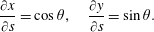 $$\begin{eqnarray}\frac{\unicode[STIX]{x2202}x}{\unicode[STIX]{x2202}s}=\cos \unicode[STIX]{x1D703},\quad \frac{\unicode[STIX]{x2202}y}{\unicode[STIX]{x2202}s}=\sin \unicode[STIX]{x1D703}.\end{eqnarray}$$
To solve the system (2.1)–(2.3), one requires initial conditions for
 $\unicode[STIX]{x1D703}(s,0)=\unicode[STIX]{x1D703}_{0}(s)$
and
 $h(s,0)=h_{0}(s)$
, as well as four boundary conditions, since the integration functions
 $A(t)$
and
 $B(t)$
must also be found as part of the solution. Suitable boundary conditions usually amount to specifying four out of: the position of each end of the viscida; the inclination angle
 $\unicode[STIX]{x1D703}$
and/or the bending moment
 $M$
applied at each end; and the tensions
 $A$
and
 $B$
. We will illustrate some typical examples below.
To facilitate computing the material derivatives in (2.2) and (2.3), we now move to a Lagrangian frame, with coordinates
 $(\unicode[STIX]{x1D709},\unicode[STIX]{x1D70F})$
such that
 $t=\unicode[STIX]{x1D70F}$
and
 $\unicode[STIX]{x1D709}$
labels a particular material section of the viscida. Enforcing local mass conservation provides a kinematic relation between
 $s$
and
 $\unicode[STIX]{x1D709}$
, namely
 $$\begin{eqnarray}\frac{\unicode[STIX]{x2202}s}{\unicode[STIX]{x2202}\unicode[STIX]{x1D709}}=\frac{h_{0}(\unicode[STIX]{x1D709})}{h(\unicode[STIX]{x1D709},\unicode[STIX]{x1D70F})}.\end{eqnarray}$$
In terms of the dimensionless Lagrangian framework, the thickness equation (2.3) becomes
 $$\begin{eqnarray}\frac{\unicode[STIX]{x2202}h}{\unicode[STIX]{x2202}\unicode[STIX]{x1D70F}}=\frac{1}{2},\end{eqnarray}$$
which may be integrated to give
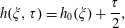 $$\begin{eqnarray}h(\unicode[STIX]{x1D709},\unicode[STIX]{x1D70F})=h_{0}(\unicode[STIX]{x1D709})+\frac{\unicode[STIX]{x1D70F}}{2},\end{eqnarray}$$
where
 $h_{0}(\unicode[STIX]{x1D709})=h(\unicode[STIX]{x1D709},0)$
. Thus, the bending moment may be written as
 $$\begin{eqnarray}M=-\frac{(h_{0}(\unicode[STIX]{x1D709})+\unicode[STIX]{x1D70F}/2)^{3}}{3}\frac{\unicode[STIX]{x2202}}{\unicode[STIX]{x2202}\unicode[STIX]{x1D70F}}\left(\frac{h_{0}(\unicode[STIX]{x1D709})+\unicode[STIX]{x1D70F}/2}{h_{0}(\unicode[STIX]{x1D709})}\frac{\unicode[STIX]{x2202}\unicode[STIX]{x1D703}}{\unicode[STIX]{x2202}\unicode[STIX]{x1D709}}\right),\end{eqnarray}$$
and the Lagrangian form of the evolution equation (2.1) is
 $$\begin{eqnarray}\frac{\unicode[STIX]{x2202}}{\unicode[STIX]{x2202}\unicode[STIX]{x1D709}}\left[(h_{0}(\unicode[STIX]{x1D709})+\unicode[STIX]{x1D70F}/2)^{3}\frac{\unicode[STIX]{x2202}}{\unicode[STIX]{x2202}\unicode[STIX]{x1D70F}}\left(\frac{h_{0}(\unicode[STIX]{x1D709})+\unicode[STIX]{x1D70F}/2}{h_{0}(\unicode[STIX]{x1D709})}\frac{\unicode[STIX]{x2202}\unicode[STIX]{x1D703}}{\unicode[STIX]{x2202}\unicode[STIX]{x1D709}}\right)\right]=\frac{3h_{0}(\unicode[STIX]{x1D709})[A(\unicode[STIX]{x1D70F})\sin \unicode[STIX]{x1D703}+B(\unicode[STIX]{x1D70F})\cos \unicode[STIX]{x1D703}]}{h_{0}(\unicode[STIX]{x1D709})+\unicode[STIX]{x1D70F}/2}.\end{eqnarray}$$
The Lagrangian spatial coordinate lies in the fixed range
 $\unicode[STIX]{x1D709}\in [0,1]$
(by our non-dimensionalization), and the evolving Eulerian length of the viscida is then given by
 $$\begin{eqnarray}L(\unicode[STIX]{x1D70F})=\int _{0}^{1}\frac{h_{0}(\unicode[STIX]{x1D709})\,\text{d}\unicode[STIX]{x1D709}}{h_{0}(\unicode[STIX]{x1D709})+\unicode[STIX]{x1D70F}/2}.\end{eqnarray}$$
Solutions of (2.9) were obtained by Griffiths & Howell (Reference Griffiths and Howell2007) for the case of a single spatially uniform viscida which forms a closed loop, so that
 $h_{0}(\unicode[STIX]{x1D709})\equiv 1$
and
 $\unicode[STIX]{x1D703}(\unicode[STIX]{x1D709},\unicode[STIX]{x1D70F})$
satisfies periodic boundary conditions
 $\unicode[STIX]{x1D703}(\unicode[STIX]{x1D709}+1,\unicode[STIX]{x1D70F})\equiv \unicode[STIX]{x1D703}(\unicode[STIX]{x1D709},\unicode[STIX]{x1D70F})+2\unicode[STIX]{x03C0}$
. In the following sections, we generalize this previous work in several ways. First we analyse situations where two or more spatially uniform viscidas are connected at a junction. We then use the results of this analysis to construct a general network model for a system of connected viscidas and junctions, as in the cross-section of a MOF consisting of closely spaced holes separated by thin glass struts. Finally, we consider the effects of thickness variations and, in particular, how they interact with angle variations in the vicinity of a junction.
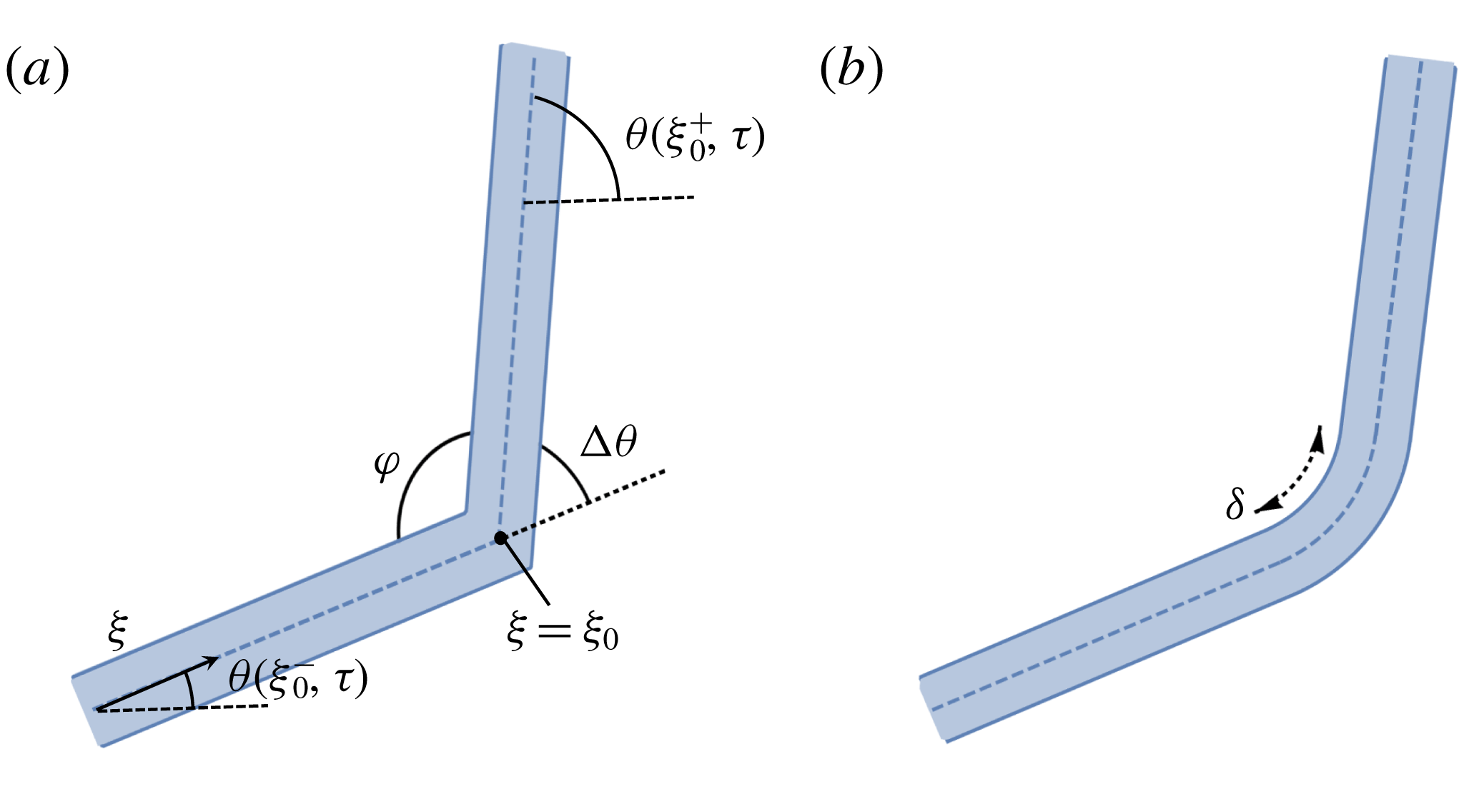
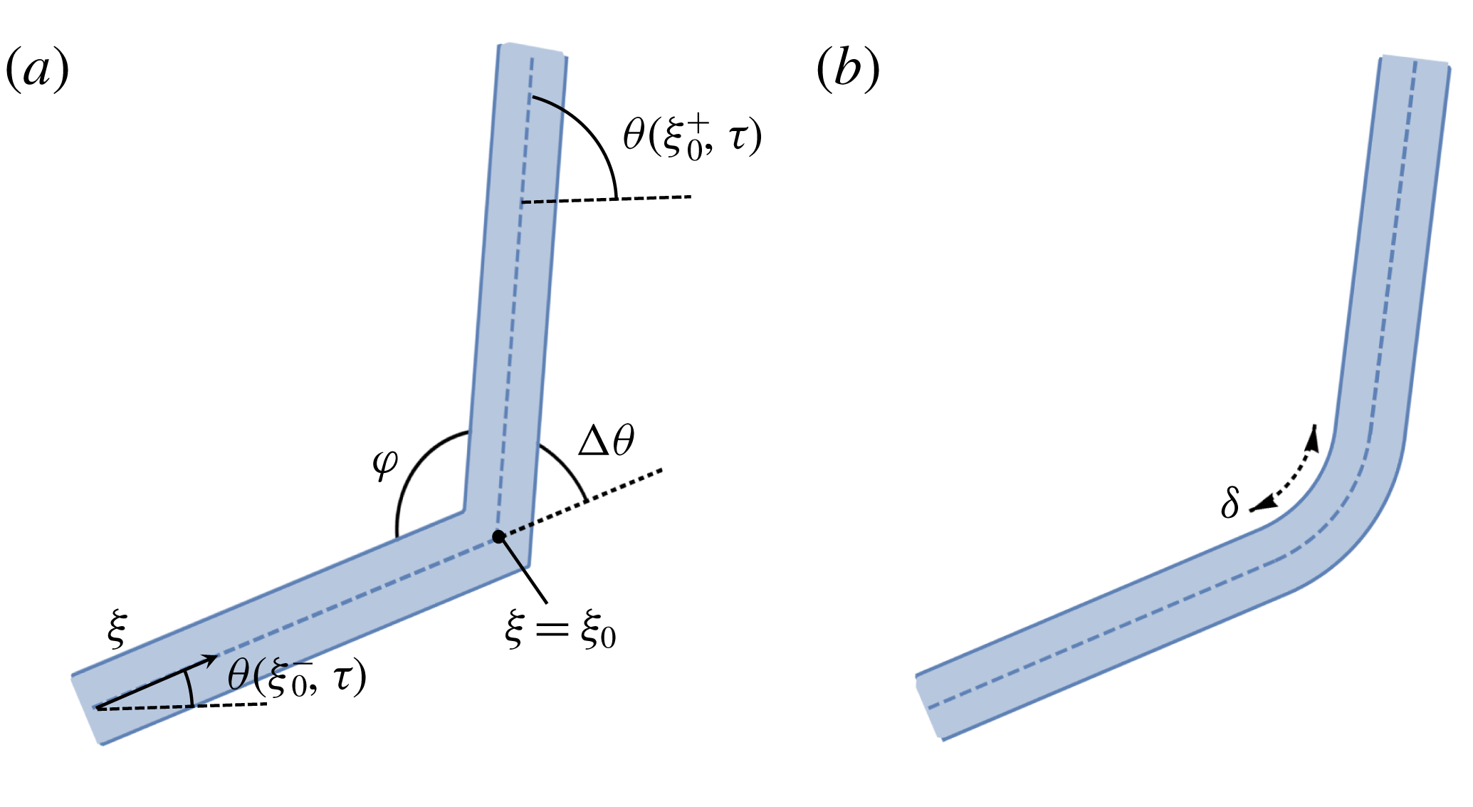
(a) A two-viscida junction with exterior angle
 $\unicode[STIX]{x0394}\unicode[STIX]{x1D703}=\unicode[STIX]{x1D703}(\unicode[STIX]{x1D709}_{0}^{+},\unicode[STIX]{x1D70F})-\unicode[STIX]{x1D703}(\unicode[STIX]{x1D709}_{0}^{-},\unicode[STIX]{x1D70F})$
and interior angle
 $\unicode[STIX]{x1D711}=\unicode[STIX]{x03C0}-\unicode[STIX]{x1D703}(\unicode[STIX]{x1D709}_{0}^{+},\unicode[STIX]{x1D70F})$
. (b) The same junction smoothed over a small length scale
 $\unicode[STIX]{x1D6FF}$
.
It is surprising at first glance that the evolution equation (2.9) makes sense whether solved forwards or backwards in time. In the ‘forward’ problem, we specify the initial geometry of the viscida and then track how it evolves, while the ‘backward’ problem consists of specifying a desired final shape of the viscida and then determining the initial conditions required to achieve it. As shown by Griffiths & Howell (Reference Griffiths and Howell2007), the resulting inverse problem is well posed until such (negative) time that either the viscida self-intersects or the thickness
 $h$
reaches zero.
3 The evolution of a viscida junction
3.1 A two-viscida junction
To gain an understanding of the general behaviour at a junction, we first analyse a join between two viscidas of uniform and equal thickness, as shown schematically in figure 5(a). Our aim is to determine the time evolution of the interior corner angle
 $\unicode[STIX]{x1D711}(\unicode[STIX]{x1D70F})=\unicode[STIX]{x03C0}+\unicode[STIX]{x1D703}(\unicode[STIX]{x1D709}_{0}^{-},\unicode[STIX]{x1D70F})-\unicode[STIX]{x1D703}(\unicode[STIX]{x1D709}_{0}^{+},\unicode[STIX]{x1D70F})$
made between the two connected viscidas. Our initial approach is to smooth the resulting corner, modelling the junction as a single viscida in which
 $\unicode[STIX]{x1D703}$
varies rapidly as a function of
 $\unicode[STIX]{x1D709}$
, over a small neighbourhood whose size is of order
 $\unicode[STIX]{x1D6FF}\ll 1$
, as in figure 5(b). The thin-viscida approximation remains valid locally provided
 $\unicode[STIX]{x1D716}\ll \unicode[STIX]{x1D6FF}$
; however, Griffiths & Howell (Reference Griffiths and Howell2007) showed that the problem may be solved for arbitrarily small
 $\unicode[STIX]{x1D6FF}$
without introducing any artefacts from the corner, and the solution approaches a well-defined limit as
 $\unicode[STIX]{x1D6FF}\rightarrow 0$
.
Since the initial thickness is assumed to be uniform, we have
 $h_{0}(\unicode[STIX]{x1D709})=1$
, so the thickness evolves as
 $h=1+\unicode[STIX]{x1D70F}/2$
from (2.7), and the evolution equation (2.9) is then simply
 $$\begin{eqnarray}\frac{\unicode[STIX]{x2202}}{\unicode[STIX]{x2202}\unicode[STIX]{x1D70F}}\left[(1+\unicode[STIX]{x1D70F}/2)\frac{\unicode[STIX]{x2202}^{2}\unicode[STIX]{x1D703}}{\unicode[STIX]{x2202}\unicode[STIX]{x1D709}^{2}}\right]=\frac{3A(\unicode[STIX]{x1D70F})}{(1+\unicode[STIX]{x1D70F}/2)^{4}}\sin \unicode[STIX]{x1D703}+\frac{3B(\unicode[STIX]{x1D70F})}{(1+\unicode[STIX]{x1D70F}/2)^{4}}\cos \unicode[STIX]{x1D703}.\end{eqnarray}$$
We rescale into the corner region via
 $\unicode[STIX]{x1D709}=\unicode[STIX]{x1D709}_{0}^{+}\unicode[STIX]{x1D6FF}\unicode[STIX]{x1D702}$
and define
 $\unicode[STIX]{x1D6E9}(\unicode[STIX]{x1D702},\unicode[STIX]{x1D70F}):=\unicode[STIX]{x1D703}(\unicode[STIX]{x1D6FF}\unicode[STIX]{x1D702},\unicode[STIX]{x1D70F})$
within this region. Substituting this local scaling into (3.1) and retaining only leading-order terms in
 $\unicode[STIX]{x1D6FF}$
gives
 $$\begin{eqnarray}\frac{\unicode[STIX]{x2202}}{\unicode[STIX]{x2202}\unicode[STIX]{x1D70F}}\left[(1+\unicode[STIX]{x1D70F}/2)\frac{\unicode[STIX]{x2202}^{2}\unicode[STIX]{x1D6E9}}{\unicode[STIX]{x2202}\unicode[STIX]{x1D702}^{2}}\right]=0,\end{eqnarray}$$
which is subject to the matching conditions
 $$\begin{eqnarray}\unicode[STIX]{x1D6E9}(\unicode[STIX]{x1D702},\unicode[STIX]{x1D70F})\rightarrow \unicode[STIX]{x1D703}(\unicode[STIX]{x1D709}_{0}^{\pm },\unicode[STIX]{x1D70F})\quad \text{as }\unicode[STIX]{x1D702}\rightarrow \pm \infty .\end{eqnarray}$$
We integrate (3.2) and apply the far-field conditions (3.3) to obtain
 $$\begin{eqnarray}\unicode[STIX]{x1D711}(\unicode[STIX]{x1D70F})=\unicode[STIX]{x03C0}-\frac{\unicode[STIX]{x03C0}-\unicode[STIX]{x1D711}(0)}{1+\unicode[STIX]{x1D70F}/2}.\end{eqnarray}$$
Therefore the junction angle straightens out with increasing
 $\unicode[STIX]{x1D70F}$
, approaching
 $\unicode[STIX]{x03C0}$
as
 $\unicode[STIX]{x1D70F}\rightarrow \infty$
. The result (3.4) also makes sense for inverse time provided
 $\unicode[STIX]{x1D70F}>-2$
, and we see that the internal angle sharpens for decreasing
 $\unicode[STIX]{x1D70F}$
, becoming zero when
 $\unicode[STIX]{x1D70F}=-2\unicode[STIX]{x1D711}(0)/\unicode[STIX]{x03C0}$
, corresponding to eventual self-intersection.
3.2 A junction of
 $n$
viscidas

We now attempt to extend our theory to describe the evolution of a junction where several viscidas meet. Let us first consider an alternative derivation of (3.4) governing the interior angle at a junction between two viscidas with uniform and equal thickness meeting with interior angle
 $\unicode[STIX]{x1D711}$
and exterior angle
 $\unicode[STIX]{x0394}\unicode[STIX]{x1D703}=\unicode[STIX]{x03C0}-\unicode[STIX]{x1D711}$
, as shown in figure 5(a). As above, we can treat the two viscidas as a single continuous viscida containing a local jump in the inclination angle
 $\unicode[STIX]{x1D703}$
, at
 $\unicode[STIX]{x1D709}=\unicode[STIX]{x1D709}_{0}$
, say. From (2.8), we know that the bending moment is given by
 $$\begin{eqnarray}M=-\frac{(1+\unicode[STIX]{x1D70F}/2)^{3}}{3}\frac{\unicode[STIX]{x2202}}{\unicode[STIX]{x2202}\unicode[STIX]{x1D70F}}\left[\left(1+\frac{\unicode[STIX]{x1D70F}}{2}\right)\frac{\unicode[STIX]{x2202}\unicode[STIX]{x1D703}}{\unicode[STIX]{x2202}\unicode[STIX]{x1D709}}\right].\end{eqnarray}$$
Since
 $\unicode[STIX]{x1D703}\sim \unicode[STIX]{x1D703}(\unicode[STIX]{x1D709}_{0}^{-},\unicode[STIX]{x1D70F})+\unicode[STIX]{x0394}\unicode[STIX]{x1D703}{\mathcal{H}}(\unicode[STIX]{x1D709}-\unicode[STIX]{x1D709}_{0})$
, near the corner, where
 ${\mathcal{H}}$
is the Heaviside function, the local bending moment behaves as
 $$\begin{eqnarray}M\sim -\frac{(1+\unicode[STIX]{x1D70F}/2)^{3}}{3}\frac{\unicode[STIX]{x2202}}{\unicode[STIX]{x2202}\unicode[STIX]{x1D70F}}\left[\left(1+\frac{\unicode[STIX]{x1D70F}}{2}\right)\unicode[STIX]{x0394}\unicode[STIX]{x1D703}\right]\unicode[STIX]{x1D6FF}(\unicode[STIX]{x1D709}-\unicode[STIX]{x1D709}_{0}),\end{eqnarray}$$
where
 $\unicode[STIX]{x1D6FF}(\unicode[STIX]{x1D709}-\unicode[STIX]{x1D709}_{0})$
denotes the Dirac delta function. To avoid an unbalanced point singularity in
 $M$
, we must therefore have
 $$\begin{eqnarray}\frac{\unicode[STIX]{x2202}}{\unicode[STIX]{x2202}\unicode[STIX]{x1D70F}}\left[\left(1+\frac{\unicode[STIX]{x1D70F}}{2}\right)\unicode[STIX]{x0394}\unicode[STIX]{x1D703}\right]=0,\end{eqnarray}$$
which upon integration with respect to
 $\unicode[STIX]{x1D70F}$
and use of
 $\unicode[STIX]{x1D711}=\unicode[STIX]{x03C0}-\unicode[STIX]{x0394}\unicode[STIX]{x1D703}$
, yields precisely the same angle evolution law (3.4) as found above by smoothing the corner.
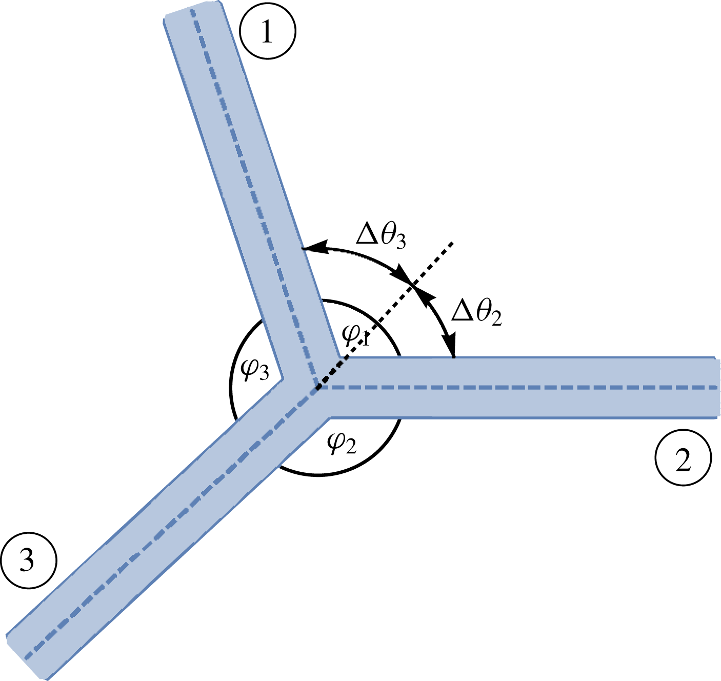
A junction between three viscidas of equal thicknesses. The behaviour is characterized by the evolution of the internal angles
 $\unicode[STIX]{x1D711}_{i}$
(
 $i=1,2,3$
).
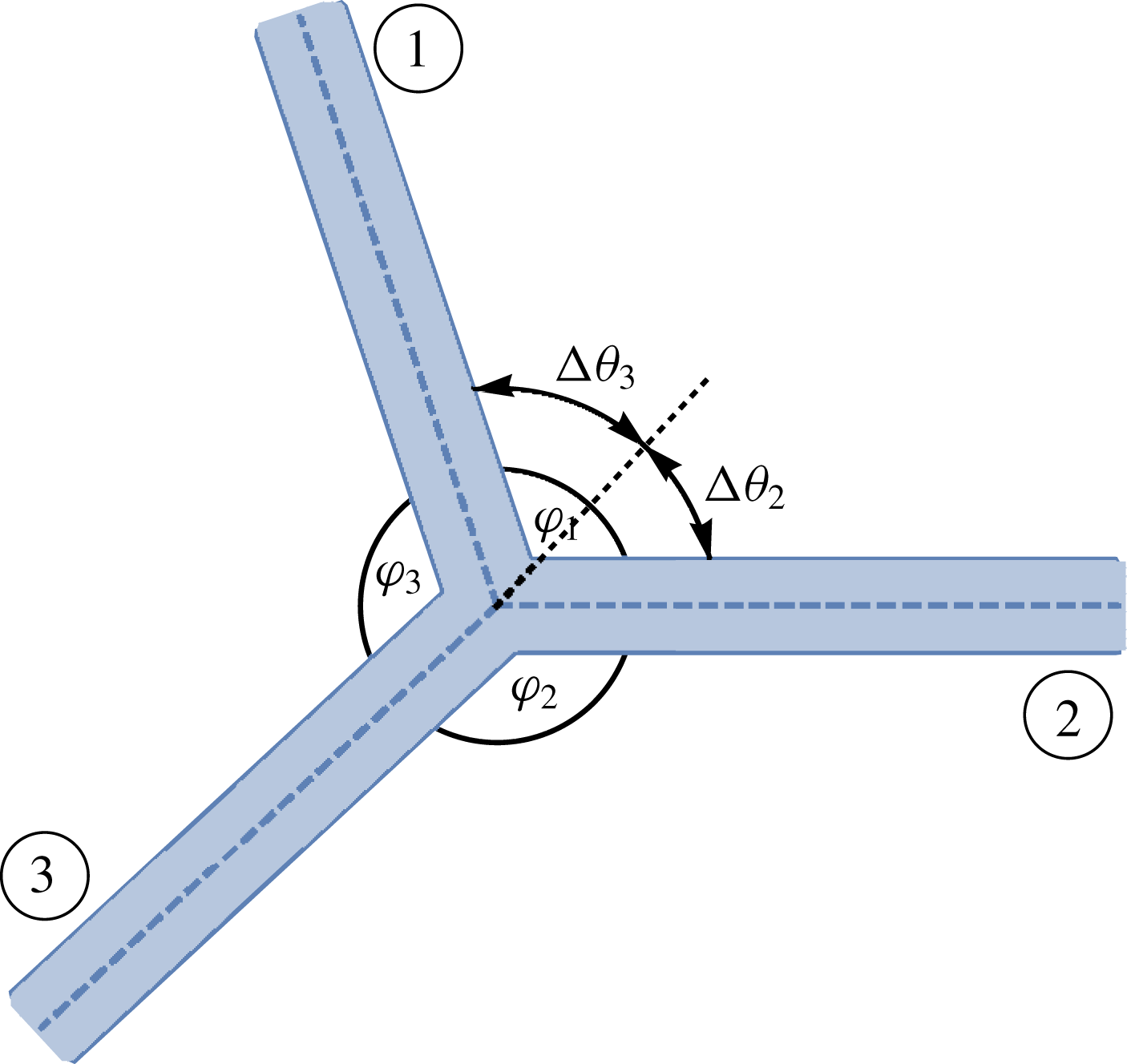
We now generalize the above argument to the case of a junction where three viscidas meet, as shown schematically in figure 6. Here the viscidas are labelled 1–3, with
 $\unicode[STIX]{x1D711}_{i}$
denoting the interior angle between viscida
 $i$
and viscida
 $i+1$
(mod 3). The bend through an exterior angle
 $\unicode[STIX]{x0394}\unicode[STIX]{x1D703}_{3}$
between viscidas 3 and 1 produces a point anticlockwise moment of magnitude
 $$\begin{eqnarray}M_{3}=-\frac{(1+\unicode[STIX]{x1D70F}/2)^{3}}{3}\frac{\unicode[STIX]{x2202}}{\unicode[STIX]{x2202}\unicode[STIX]{x1D70F}}\left[\left(1+\frac{\unicode[STIX]{x1D70F}}{2}\right)\unicode[STIX]{x0394}\unicode[STIX]{x1D703}_{3}\right].\end{eqnarray}$$
Similarly, the bend between viscidas 3 and 2 produces a point moment of magnitude
 $$\begin{eqnarray}M_{2}=\frac{(1+\unicode[STIX]{x1D70F}/2)^{3}}{3}\frac{\unicode[STIX]{x2202}}{\unicode[STIX]{x2202}\unicode[STIX]{x1D70F}}\left[\left(1+\frac{\unicode[STIX]{x1D70F}}{2}\right)\unicode[STIX]{x0394}\unicode[STIX]{x1D703}_{2}\right].\end{eqnarray}$$
To ensure that no unbalanced point moment acts on viscida 3, we must have
 $M_{3}+M_{2}=0$
, which may be simplified to
 $$\begin{eqnarray}\frac{\unicode[STIX]{x2202}}{\unicode[STIX]{x2202}\unicode[STIX]{x1D70F}}\left[\left(1+\frac{\unicode[STIX]{x1D70F}}{2}\right)(\unicode[STIX]{x1D711}_{3}-\unicode[STIX]{x1D711}_{2})\right]=0.\end{eqnarray}$$
Similarly, a balance of moments acting on each of viscidas 1 and 2 gives
 $$\begin{eqnarray}\frac{\unicode[STIX]{x2202}}{\unicode[STIX]{x2202}\unicode[STIX]{x1D70F}}\left[\left(1+\frac{\unicode[STIX]{x1D70F}}{2}\right)(\unicode[STIX]{x1D711}_{1}-\unicode[STIX]{x1D711}_{3})\right]=0\quad \text{and}\quad \frac{\unicode[STIX]{x2202}}{\unicode[STIX]{x2202}\unicode[STIX]{x1D70F}}\left[\left(1+\frac{\unicode[STIX]{x1D70F}}{2}\right)(\unicode[STIX]{x1D711}_{2}-\unicode[STIX]{x1D711}_{1})\right]=0.\end{eqnarray}$$
We also note that the interior angles must satisfy
 $$\begin{eqnarray}\unicode[STIX]{x1D711}_{1}+\unicode[STIX]{x1D711}_{2}+\unicode[STIX]{x1D711}_{3}=2\unicode[STIX]{x03C0}.\end{eqnarray}$$
Using (3.12) and combinations of (3.10) and (3.11), we find that
 $$\begin{eqnarray}\unicode[STIX]{x1D711}_{i}(\unicode[STIX]{x1D70F})=\frac{2\unicode[STIX]{x03C0}}{3}+\frac{\unicode[STIX]{x1D711}_{i}(0)-2\unicode[STIX]{x03C0}/3}{1+\unicode[STIX]{x1D70F}/2},\end{eqnarray}$$
where
 $i\in \{1,2,3\}$
. Therefore, the junction of three viscidas evolves in a way that ensures that, as
 $\unicode[STIX]{x1D70F}\rightarrow \infty$
, the interior angles
 $\unicode[STIX]{x1D711}_{1},\unicode[STIX]{x1D711}_{2},\unicode[STIX]{x1D711}_{3}$
all tend to
 $2\unicode[STIX]{x03C0}/3$
.
We hypothesize, based on the examples we have shown, that this method is generalizable for a junction of
 $n$
viscidas, for any
 $n\geqslant 2$
. Balancing moments at the
 $n$
-viscida junction yields, after some algebra,
 $$\begin{eqnarray}\frac{\unicode[STIX]{x2202}}{\unicode[STIX]{x2202}\unicode[STIX]{x1D70F}}\left[\left(1+\frac{\unicode[STIX]{x1D70F}}{2}\right)(\unicode[STIX]{x1D711}_{i}-\unicode[STIX]{x1D711}_{j})\right]=0,\end{eqnarray}$$
for all
 $1\leqslant i<j\leqslant n$
, where
 $\unicode[STIX]{x1D711}_{i}$
again labels the interior angle between viscidas
 $i$
and
 $i+1$
(mod
 $n$
). Also, in the general case, the relation (3.12) becomes
 $$\begin{eqnarray}\mathop{\sum }_{i=1}^{n}\unicode[STIX]{x1D711}_{i}=2\unicode[STIX]{x03C0},\end{eqnarray}$$
which in combination with (3.14), gives
 $$\begin{eqnarray}\unicode[STIX]{x1D711}_{i}(\unicode[STIX]{x1D70F})=\frac{2\unicode[STIX]{x03C0}}{n}+\frac{\unicode[STIX]{x1D711}_{i}(0)-2\unicode[STIX]{x03C0}/n}{1+\unicode[STIX]{x1D70F}/2}.\end{eqnarray}$$
Again, all the interior angles tend to the same value,
 $2\unicode[STIX]{x03C0}/n$
, as
 $\unicode[STIX]{x1D70F}\rightarrow \infty$
.
4 Modelling a viscida network
4.1 A two-viscida network
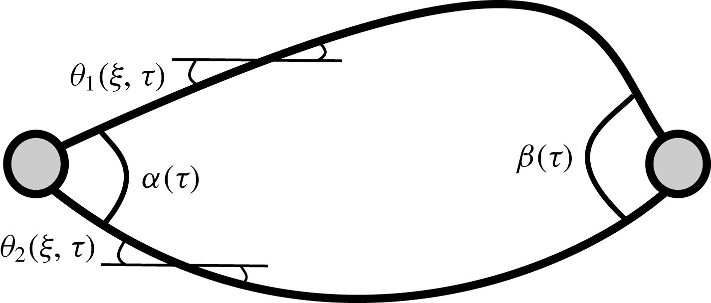
Schematic diagram of the two-viscida problem. The top viscida has a centreline described by
 $\unicode[STIX]{x1D703}_{1}(\unicode[STIX]{x1D709},\unicode[STIX]{x1D70F})$
and the bottom viscida has a centreline described by
 $\unicode[STIX]{x1D703}_{2}(\unicode[STIX]{x1D709},\unicode[STIX]{x1D70F})$
. The interior angle at
 $\unicode[STIX]{x1D709}=0$
for any time
 $\unicode[STIX]{x1D70F}$
is given by
 $\unicode[STIX]{x1D6FC}(\unicode[STIX]{x1D70F})$
and the angle at
 $\unicode[STIX]{x1D709}=1$
by
 $\unicode[STIX]{x1D6FD}(\unicode[STIX]{x1D70F})$
. The two nodes represent the viscida junctions.
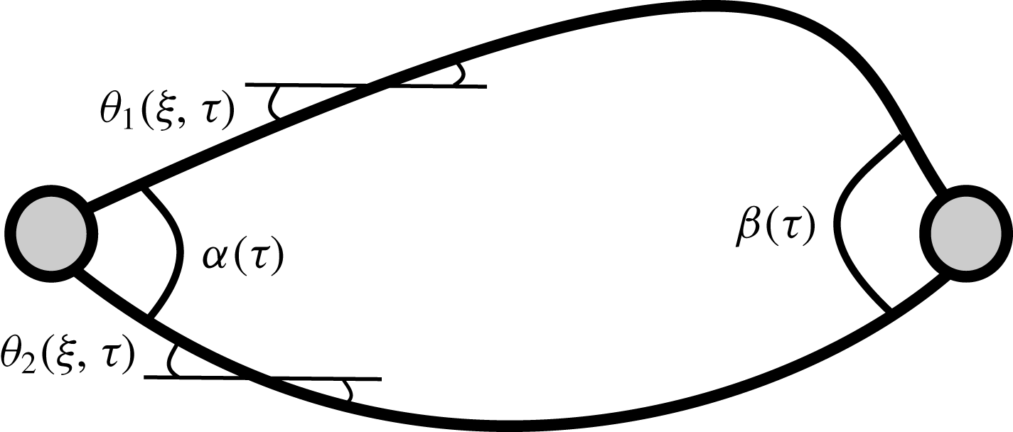
In this section, we analyse a set-up consisting of two interacting viscidas of equal and uniform thickness, connected by junctions at their ends, as illustrated in figure 7. By combining the governing equation (3.1) for each viscida with the angle evolution equation (3.4) for each node, we obtain a closed model for the coupled system of viscidas and junctions. The ideas developed in this section will be generalized below to a more general network of viscidas connected by junctions.
The inclination angle
 $\unicode[STIX]{x1D703}_{i}(\unicode[STIX]{x1D709},\unicode[STIX]{x1D70F})$
in viscida
 $i\in \{1,2\}$
satisfies (3.1), which we write in the form
 $$\begin{eqnarray}\frac{\unicode[STIX]{x2202}}{\unicode[STIX]{x2202}\unicode[STIX]{x1D70F}}\left[\left(1+\frac{\unicode[STIX]{x1D70F}}{2}\right)\frac{\unicode[STIX]{x2202}^{2}\unicode[STIX]{x1D703}_{i}}{\unicode[STIX]{x2202}\unicode[STIX]{x1D709}^{2}}\right]=A_{i}(\unicode[STIX]{x1D70F})\sin \unicode[STIX]{x1D703}_{i}+B_{i}(\unicode[STIX]{x1D70F})\cos \unicode[STIX]{x1D703}_{i},\end{eqnarray}$$
by absorbing factors
 $\pm 3/(1+\unicode[STIX]{x1D70F}/2)^{4}$
into the functions
 $A_{i}(\unicode[STIX]{x1D70F})$
and
 $B_{i}(\unicode[STIX]{x1D70F})$
. Since each equation (4.1) is second order in space and has two additional unknowns, eight boundary conditions are needed in total to close the problem.
To ensure that the ends join up, we impose
 $$\begin{eqnarray}\int _{0}^{1}\cos \unicode[STIX]{x1D703}_{1}\,\text{d}\unicode[STIX]{x1D709}=\int _{0}^{1}\cos \unicode[STIX]{x1D703}_{2}\,\text{d}\unicode[STIX]{x1D709}\quad \text{and}\quad \int _{0}^{1}\sin \unicode[STIX]{x1D703}_{1}\,\text{d}\unicode[STIX]{x1D709}=\int _{0}^{1}\sin \unicode[STIX]{x1D703}_{2}\,\text{d}\unicode[STIX]{x1D709}.\end{eqnarray}$$
It is further required that, at each junction, there is zero net bending moment, i.e.
 $M_{1}+M_{2}=0$
where the bending moment in each viscida is given by (3.5). Therefore we impose the boundary condition
 $$\begin{eqnarray}\frac{\unicode[STIX]{x2202}}{\unicode[STIX]{x2202}\unicode[STIX]{x1D70F}}\left[(1+\unicode[STIX]{x1D70F}/2)\left(\frac{\unicode[STIX]{x2202}\unicode[STIX]{x1D703}_{1}}{\unicode[STIX]{x2202}\unicode[STIX]{x1D709}}+\frac{\unicode[STIX]{x2202}\unicode[STIX]{x1D703}_{2}}{\unicode[STIX]{x2202}\unicode[STIX]{x1D709}}\right)\right]=0\quad \text{at }\unicode[STIX]{x1D709}=0,1.\end{eqnarray}$$
Equation (3.4) provides the evolution of the corners at
 $\unicode[STIX]{x1D709}=0,1$
,
 $$\begin{eqnarray}\displaystyle & \displaystyle \unicode[STIX]{x1D6FC}(\unicode[STIX]{x1D70F})=\unicode[STIX]{x03C0}+\frac{\unicode[STIX]{x1D6FC}(0)-\unicode[STIX]{x03C0}}{1+\unicode[STIX]{x1D70F}/2}=\unicode[STIX]{x1D703}_{1}(0,\unicode[STIX]{x1D70F})-\unicode[STIX]{x1D703}_{2}(0,\unicode[STIX]{x1D70F}), & \displaystyle\end{eqnarray}$$
 $$\begin{eqnarray}\displaystyle & \displaystyle \unicode[STIX]{x1D6FD}(\unicode[STIX]{x1D70F})=\unicode[STIX]{x03C0}+\frac{\unicode[STIX]{x1D6FD}(0)-\unicode[STIX]{x03C0}}{1+\unicode[STIX]{x1D70F}/2}=\unicode[STIX]{x1D703}_{2}(1,\unicode[STIX]{x1D70F})-\unicode[STIX]{x1D703}_{1}(1,\unicode[STIX]{x1D70F}), & \displaystyle\end{eqnarray}$$
respectively, where
 $\unicode[STIX]{x1D6FC}(0)$
is the initial internal angle at
 $\unicode[STIX]{x1D709}=0$
and
 $\unicode[STIX]{x1D6FD}(0)$
is the initial internal angle at
 $\unicode[STIX]{x1D709}=1$
. Force balances at
 $\unicode[STIX]{x1D709}=0,1$
imply that there must be zero resultant forces in the
 $x$
- and
 $y$
-direction, for all
 $\unicode[STIX]{x1D70F}$
, i.e.
 $$\begin{eqnarray}A_{1}(\unicode[STIX]{x1D70F})+A_{2}(\unicode[STIX]{x1D70F})=0\quad \text{and}\quad B_{1}(\unicode[STIX]{x1D70F})+B_{2}(\unicode[STIX]{x1D70F})=0.\end{eqnarray}$$
Equations (4.2)–(4.6) provide eight boundary conditions in total, and so appear to close the problem. However, there remains an indeterminate rigid-body motion: for example, one can easily see that the entire problem (4.1)–(4.6) is invariant under the transformation
 $\unicode[STIX]{x1D703}_{i}(\unicode[STIX]{x1D709},\unicode[STIX]{x1D70F})\mapsto \unicode[STIX]{x1D703}_{i}(\unicode[STIX]{x1D709},\unicode[STIX]{x1D70F})+\unicode[STIX]{x1D713}(\unicode[STIX]{x1D70F})$
for any function
 $\unicode[STIX]{x1D713}(\unicode[STIX]{x1D70F})$
. Therefore, we will find that three further conditions are needed to fix the arbitrary translation and rotation.
Upon integration of (4.1) with respect to
 $\unicode[STIX]{x1D709}$
, we obtain
 $$\begin{eqnarray}\frac{\unicode[STIX]{x2202}^{2}}{\unicode[STIX]{x2202}\unicode[STIX]{x1D709}\unicode[STIX]{x2202}\unicode[STIX]{x1D70F}}\left[\left(1+\frac{\unicode[STIX]{x1D70F}}{2}\right)\unicode[STIX]{x1D703}_{i}\right]=A_{i}(\unicode[STIX]{x1D70F})Y_{i}+B_{i}(\unicode[STIX]{x1D70F})X_{i}+C_{i}(\unicode[STIX]{x1D70F}),\end{eqnarray}$$
where
 $$\begin{eqnarray}\left(\begin{array}{@{}c@{}}X_{i}(\unicode[STIX]{x1D709},\unicode[STIX]{x1D70F})\\ Y_{i}(\unicode[STIX]{x1D709},\unicode[STIX]{x1D70F})\end{array}\right)=(1+\unicode[STIX]{x1D70F}/2)\left(\begin{array}{@{}c@{}}x_{i}(s,t)\\ y_{i}(s,t)\end{array}\right)=\left(\begin{array}{@{}c@{}}X_{0}(\unicode[STIX]{x1D70F})\\ Y_{0}(\unicode[STIX]{x1D70F})\end{array}\right)+\int _{0}^{\unicode[STIX]{x1D709}}\left(\begin{array}{@{}c@{}}\cos \unicode[STIX]{x1D703}_{i}(\hat{\unicode[STIX]{x1D709}},\unicode[STIX]{x1D70F})\\ \sin \unicode[STIX]{x1D703}_{i}(\hat{\unicode[STIX]{x1D709}},\unicode[STIX]{x1D70F})\end{array}\right)\text{d}\hat{\unicode[STIX]{x1D709}}\end{eqnarray}$$
gives the centreline of viscida
 $i\in \{1,2\}$
, expressed in Lagrangian variables. At
 $\unicode[STIX]{x1D709}=0$
, the two viscidas meet at a junction whose position
 $(X_{0}(\unicode[STIX]{x1D70F}),Y_{0}(\unicode[STIX]{x1D70F}))$
is thus far arbitrary. By applying (4.3) and (4.6) at
 $\unicode[STIX]{x1D709}=0$
, we deduce that
 $$\begin{eqnarray}C_{1}(\unicode[STIX]{x1D70F})+C_{2}(\unicode[STIX]{x1D70F})=0,\end{eqnarray}$$
and then the corresponding moment balance (4.3) at
 $\unicode[STIX]{x1D709}=1$
is satisfied identically: a manifestation of the rotational invariance alluded to above.
Integration once more with respect to
 $\unicode[STIX]{x1D709}$
gives
 $$\begin{eqnarray}\frac{\unicode[STIX]{x2202}}{\unicode[STIX]{x2202}\unicode[STIX]{x1D70F}}\left[\left(1+\frac{\unicode[STIX]{x1D70F}}{2}\right)\unicode[STIX]{x1D703}_{i}\right]=A_{i}(\unicode[STIX]{x1D70F})\int _{0}^{\unicode[STIX]{x1D709}}Y_{i}\,\text{d}\hat{\unicode[STIX]{x1D709}}+B_{i}(\unicode[STIX]{x1D70F})\int _{0}^{\unicode[STIX]{x1D709}}X_{i}\,\text{d}\hat{\unicode[STIX]{x1D709}}+C_{i}(\unicode[STIX]{x1D70F})\unicode[STIX]{x1D709}+D_{i}(\unicode[STIX]{x1D70F}),\end{eqnarray}$$
for
 $i\in \{1,2\}$
. If we subtract (4.10) with
 $i=1$
from (4.10) with
 $i=2$
and use the angle conditions (4.4) and (4.5) at
 $\unicode[STIX]{x1D709}=0$
and
 $\unicode[STIX]{x1D709}=1$
, we obtain the relations
 $$\begin{eqnarray}\displaystyle & \displaystyle D_{1}(\unicode[STIX]{x1D70F})-D_{2}(\unicode[STIX]{x1D70F})=\frac{\unicode[STIX]{x03C0}}{2}, & \displaystyle\end{eqnarray}$$
 $$\begin{eqnarray}\displaystyle & \displaystyle C_{1}(\unicode[STIX]{x1D70F})={\textstyle \frac{1}{2}}[A_{2}(\unicode[STIX]{x1D70F})\overline{Y_{2}}(\unicode[STIX]{x1D70F})+B_{2}(\unicode[STIX]{x1D70F})\overline{X_{2}}(\unicode[STIX]{x1D70F})-A_{1}(\unicode[STIX]{x1D70F})\overline{Y_{1}}(\unicode[STIX]{x1D70F})-B_{1}(\unicode[STIX]{x1D70F})\overline{X_{1}}(\unicode[STIX]{x1D70F})-\unicode[STIX]{x03C0}], & \displaystyle\end{eqnarray}$$
where the bar is used to denote the averaged value
 $$\begin{eqnarray}\overline{F}(\unicode[STIX]{x1D70F}):=\int _{0}^{1}F(\unicode[STIX]{x1D709},\unicode[STIX]{x1D70F})\,\text{d}\unicode[STIX]{x1D709}.\end{eqnarray}$$
At this point it is helpful to make some specific choices that eliminate the arbitrary rigid-body motion and simplify the problem somewhat. We fix the rotation by taking
 $D_{1}(\unicode[STIX]{x1D70F})+D_{2}(\unicode[STIX]{x1D70F})\equiv 0$
. We also assume that the net translation is chosen to fix the net centroid of the system, so that
 $\overline{X_{1}}(\unicode[STIX]{x1D70F})+\overline{X_{2}}(\unicode[STIX]{x1D70F})\equiv 0$
and
 $\overline{Y_{1}}(\unicode[STIX]{x1D70F})+\overline{Y_{2}}(\unicode[STIX]{x1D70F})\equiv 0$
. Given these specific choices, we can evaluate
 $$\begin{eqnarray}C_{1}=-\frac{\unicode[STIX]{x03C0}}{2},\quad C_{2}=\frac{\unicode[STIX]{x03C0}}{2},\quad D_{1}=\frac{\unicode[STIX]{x03C0}}{4},\quad D_{2}=-\frac{\unicode[STIX]{x03C0}}{4},\end{eqnarray}$$
as well as
 $$\begin{eqnarray}\displaystyle & \displaystyle \left(\begin{array}{@{}c@{}}X_{0}(\unicode[STIX]{x1D70F})\\ Y_{0}(\unicode[STIX]{x1D70F})\end{array}\right)=-\frac{1}{2}\int _{0}^{1}(1-\unicode[STIX]{x1D709})\left(\begin{array}{@{}c@{}}\cos \unicode[STIX]{x1D703}_{1}(\unicode[STIX]{x1D709},\unicode[STIX]{x1D70F})+\cos \unicode[STIX]{x1D703}_{2}(\unicode[STIX]{x1D709},\unicode[STIX]{x1D70F})\\ \sin \unicode[STIX]{x1D703}_{1}(\unicode[STIX]{x1D709},\unicode[STIX]{x1D70F})+\sin \unicode[STIX]{x1D703}_{2}(\unicode[STIX]{x1D709},\unicode[STIX]{x1D70F})\end{array}\right)\,\text{d}\unicode[STIX]{x1D709}, & \displaystyle\end{eqnarray}$$
 $$\begin{eqnarray}\displaystyle & \displaystyle \left(\begin{array}{@{}c@{}}X_{i}(1,\unicode[STIX]{x1D70F})\\ Y_{i}(1,\unicode[STIX]{x1D70F})\end{array}\right)=\frac{1}{2}\int _{0}^{1}\unicode[STIX]{x1D709}\left(\begin{array}{@{}c@{}}\cos \unicode[STIX]{x1D703}_{1}(\unicode[STIX]{x1D709},\unicode[STIX]{x1D70F})+\cos \unicode[STIX]{x1D703}_{2}(\unicode[STIX]{x1D709},\unicode[STIX]{x1D70F})\\ \sin \unicode[STIX]{x1D703}_{1}(\unicode[STIX]{x1D709},\unicode[STIX]{x1D70F})+\sin \unicode[STIX]{x1D703}_{2}(\unicode[STIX]{x1D709},\unicode[STIX]{x1D70F})\end{array}\right)\,\text{d}\unicode[STIX]{x1D709}. & \displaystyle\end{eqnarray}$$
 $$\begin{eqnarray}\frac{\unicode[STIX]{x2202}}{\unicode[STIX]{x2202}\unicode[STIX]{x1D70F}}\left[\left(1+\frac{\unicode[STIX]{x1D70F}}{2}\right)\unicode[STIX]{x1D703}_{i}\right]=(-1)^{i}\left[A_{1}(\unicode[STIX]{x1D70F})\int _{0}^{\unicode[STIX]{x1D709}}Y_{i}\,\text{d}\hat{\unicode[STIX]{x1D709}}+B_{1}(\unicode[STIX]{x1D70F})\int _{0}^{\unicode[STIX]{x1D709}}X_{i}\,\text{d}\hat{\unicode[STIX]{x1D709}}+\frac{\unicode[STIX]{x03C0}}{4}(1-2\unicode[STIX]{x1D709})\right],\end{eqnarray}$$
which can be solved numerically for
 $\unicode[STIX]{x1D703}_{i}$
once we have determined
 $A_{1}(\unicode[STIX]{x1D70F})$
and
 $B_{1}(\unicode[STIX]{x1D70F})$
.
To this end, we multiply (4.7) by
 $X_{i}$
for
 $i\in \{1,2\}$
and integrate over the viscida length to obtain
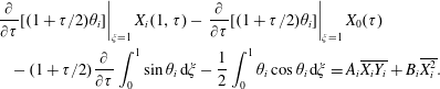 $$\begin{eqnarray}\displaystyle & & \displaystyle \left.\frac{\unicode[STIX]{x2202}}{\unicode[STIX]{x2202}\unicode[STIX]{x1D70F}}[(1+\unicode[STIX]{x1D70F}/2)\unicode[STIX]{x1D703}_{i}]\right|_{\unicode[STIX]{x1D709}=1}X_{i}(1,\unicode[STIX]{x1D70F})-\left.\frac{\unicode[STIX]{x2202}}{\unicode[STIX]{x2202}\unicode[STIX]{x1D70F}}[(1+\unicode[STIX]{x1D70F}/2)\unicode[STIX]{x1D703}_{i}]\right|_{\unicode[STIX]{x1D709}=1}X_{0}(\unicode[STIX]{x1D70F})\nonumber\\ \displaystyle & & \displaystyle \quad -\,(1+\unicode[STIX]{x1D70F}/2)\frac{\unicode[STIX]{x2202}}{\unicode[STIX]{x2202}\unicode[STIX]{x1D70F}}\int _{0}^{1}\sin \unicode[STIX]{x1D703}_{i}\,\text{d}\unicode[STIX]{x1D709}-\frac{1}{2}\int _{0}^{1}\unicode[STIX]{x1D703}_{i}\cos \unicode[STIX]{x1D703}_{i}\,\text{d}\unicode[STIX]{x1D709}=A_{i}\overline{X_{i}Y_{i}}+B_{i}\overline{X_{i}^{2}}.\end{eqnarray}$$
In a similar fashion, by multiplying (4.7) by
 $Y_{i}$
, integrating over the viscida length and using (4.2b
), we obtain
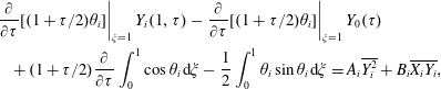 $$\begin{eqnarray}\displaystyle & & \displaystyle \left.\frac{\unicode[STIX]{x2202}}{\unicode[STIX]{x2202}\unicode[STIX]{x1D70F}}[(1+\unicode[STIX]{x1D70F}/2)\unicode[STIX]{x1D703}_{i}]\right|_{\unicode[STIX]{x1D709}=1}Y_{i}(1,\unicode[STIX]{x1D70F})-\left.\frac{\unicode[STIX]{x2202}}{\unicode[STIX]{x2202}\unicode[STIX]{x1D70F}}[(1+\unicode[STIX]{x1D70F}/2)\unicode[STIX]{x1D703}_{i}]\right|_{\unicode[STIX]{x1D709}=1}Y_{0}(\unicode[STIX]{x1D70F})\nonumber\\ \displaystyle & & \displaystyle \quad +\,(1+\unicode[STIX]{x1D70F}/2)\frac{\unicode[STIX]{x2202}}{\unicode[STIX]{x2202}\unicode[STIX]{x1D70F}}\int _{0}^{1}\cos \unicode[STIX]{x1D703}_{i}\,\text{d}\unicode[STIX]{x1D709}-\frac{1}{2}\int _{0}^{1}\unicode[STIX]{x1D703}_{i}\sin \unicode[STIX]{x1D703}_{i}\,\text{d}\unicode[STIX]{x1D709}=A_{i}\overline{Y_{i}^{2}}+B_{i}\overline{X_{i}Y_{i}},\end{eqnarray}$$
with
 $i\in \{1,2\}$
. We subtract the cases
 $i=1$
and
 $i=2$
of (4.17) and (4.18) and rearrange to obtain a linear system for
 $A_{1}$
and
 $B_{1}$
as follows:
 $$\begin{eqnarray}\displaystyle & & \displaystyle \left(\begin{array}{@{}cc@{}}\overline{X_{1}Y_{1}}+\overline{X_{2}Y_{2}} & \overline{X_{1}^{2}}+\overline{X_{2}^{2}}\\ \overline{Y_{1}^{2}}+\overline{Y_{2}^{2}} & \overline{X_{1}Y_{1}}+\overline{X_{2}Y_{2}}\end{array}\right)\left(\begin{array}{@{}c@{}}\vphantom{\overline{X_{1}^{2}}}A_{1}\\ \vphantom{\overline{X_{1}^{2}}}B_{1}\end{array}\right)\nonumber\\ \displaystyle & & \displaystyle \quad =\frac{1}{2}\int _{0}^{1}\left[\left(\begin{array}{@{}c@{}}\vphantom{\overline{X_{1}^{2}}}\cos \unicode[STIX]{x1D703}_{2}\\ \vphantom{\overline{X_{1}^{2}}}\sin \unicode[STIX]{x1D703}_{2}\end{array}\right)[\unicode[STIX]{x1D703}_{2}-\unicode[STIX]{x03C0}(\unicode[STIX]{x1D709}-1/2)]-\left(\begin{array}{@{}c@{}}\vphantom{\overline{X_{1}^{2}}}\cos \unicode[STIX]{x1D703}_{1}\\ \vphantom{\overline{X_{1}^{2}}}\sin \unicode[STIX]{x1D703}_{1}\end{array}\right)[\unicode[STIX]{x1D703}_{1}-\unicode[STIX]{x03C0}(1/2-\unicode[STIX]{x1D709})]\right]\text{d}\unicode[STIX]{x1D709}.\qquad\end{eqnarray}$$
With
 $A_{1}(\unicode[STIX]{x1D70F})$
and
 $B_{1}(\unicode[STIX]{x1D70F})$
determined at every time
 $\unicode[STIX]{x1D70F}$
by (4.19), the evolution equation (4.16) for
 $\unicode[STIX]{x1D703}_{i}(\unicode[STIX]{x1D709},\unicode[STIX]{x1D70F})$
is easily solved numerically, for example by using the method of lines. Before proceeding, we observe that the coupled problem (4.16), (4.19) admits an exact steady solution in which
 $$\begin{eqnarray}\unicode[STIX]{x1D703}_{1}(\unicode[STIX]{x1D709},\unicode[STIX]{x1D70F})=\unicode[STIX]{x03C0}\left({\textstyle \frac{1}{2}}-\unicode[STIX]{x1D709}\right),\quad \unicode[STIX]{x1D703}_{2}(\unicode[STIX]{x1D709},\unicode[STIX]{x1D70F})=\unicode[STIX]{x03C0}\left(\unicode[STIX]{x1D709}-{\textstyle \frac{1}{2}}\right).\end{eqnarray}$$
Clearly these forms render the right-hand side of (4.19) identically zero and thus give
 $A_{1}=B_{1}=0$
(since the matrix on the left-hand side of (4.19) is negative definite). Then the left- and right-hand sides of (4.16) are also identically equal. The solution (4.20) corresponds to a pair of semi-circular viscidas whose ends meet smoothly with an interior angle of
 $\unicode[STIX]{x03C0}$
, which is tantamount to a single complete circular viscida. We expect the system to converge to such a configuration for large positive values of
 $\unicode[STIX]{x1D70F}$
.
We illustrate the strategy developed above to solve for the evolution of a pair of symmetric coupled viscidas whose initial centreline geometries are defined by
 $$\begin{eqnarray}\unicode[STIX]{x1D703}_{1}(\unicode[STIX]{x1D709},0)=-\unicode[STIX]{x1D703}_{2}(\unicode[STIX]{x1D709},0)=\tanh (20(1/2-\unicode[STIX]{x1D709})).\end{eqnarray}$$
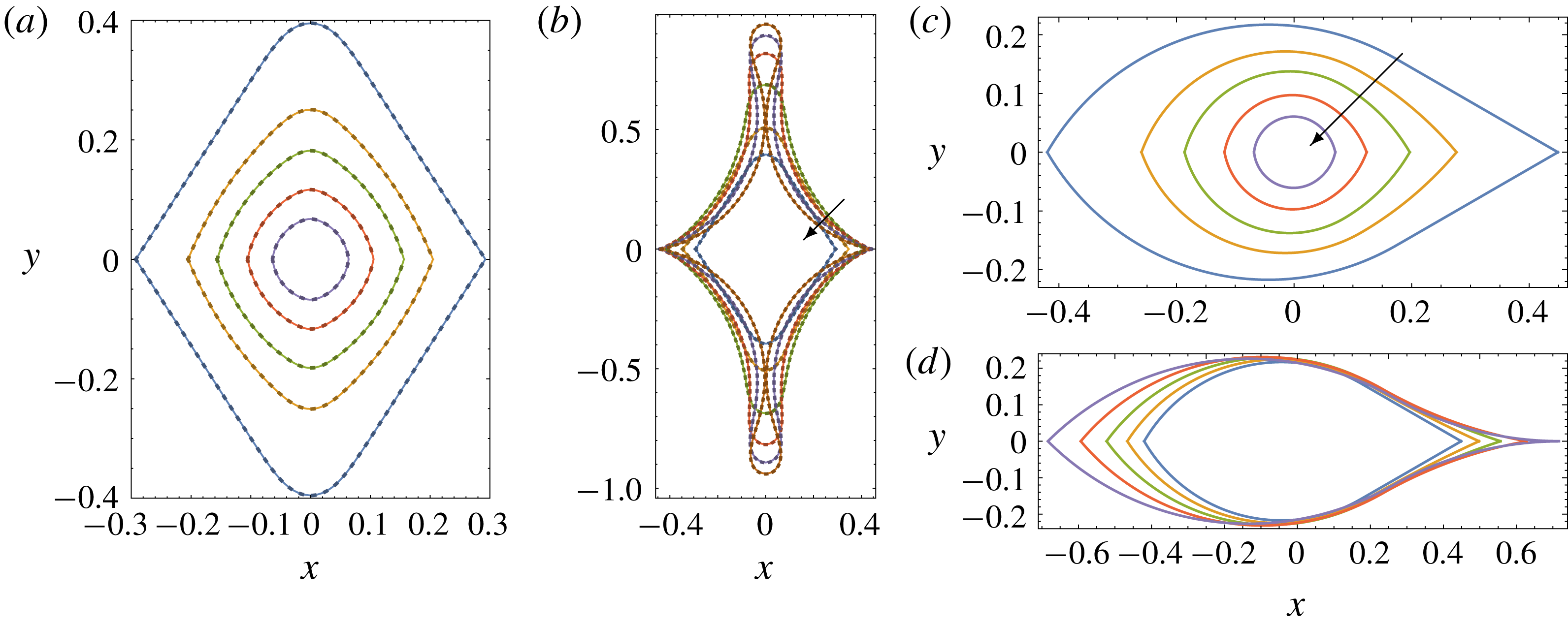
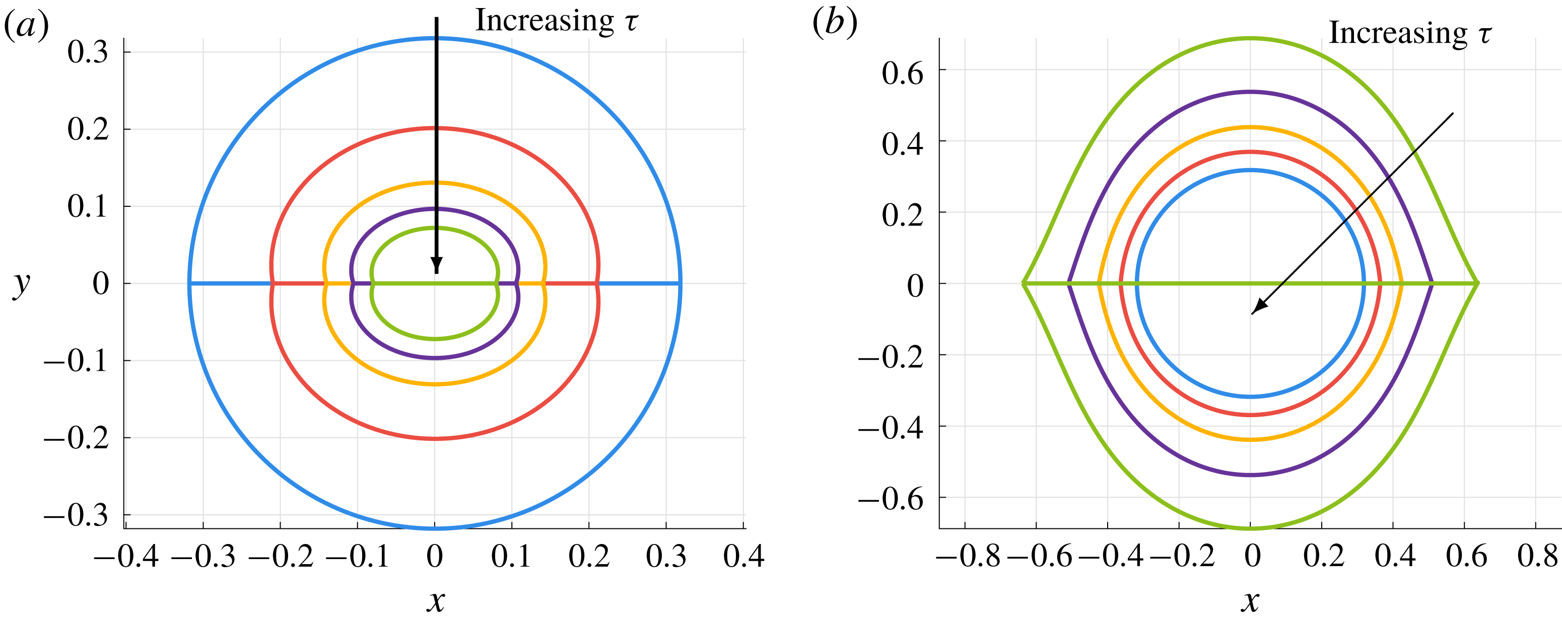
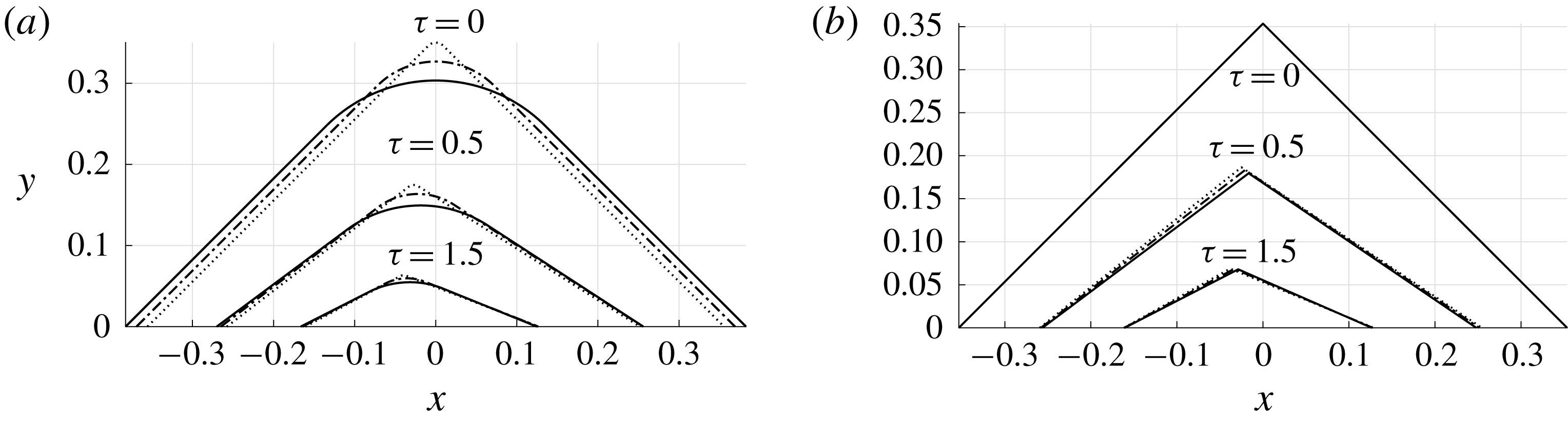
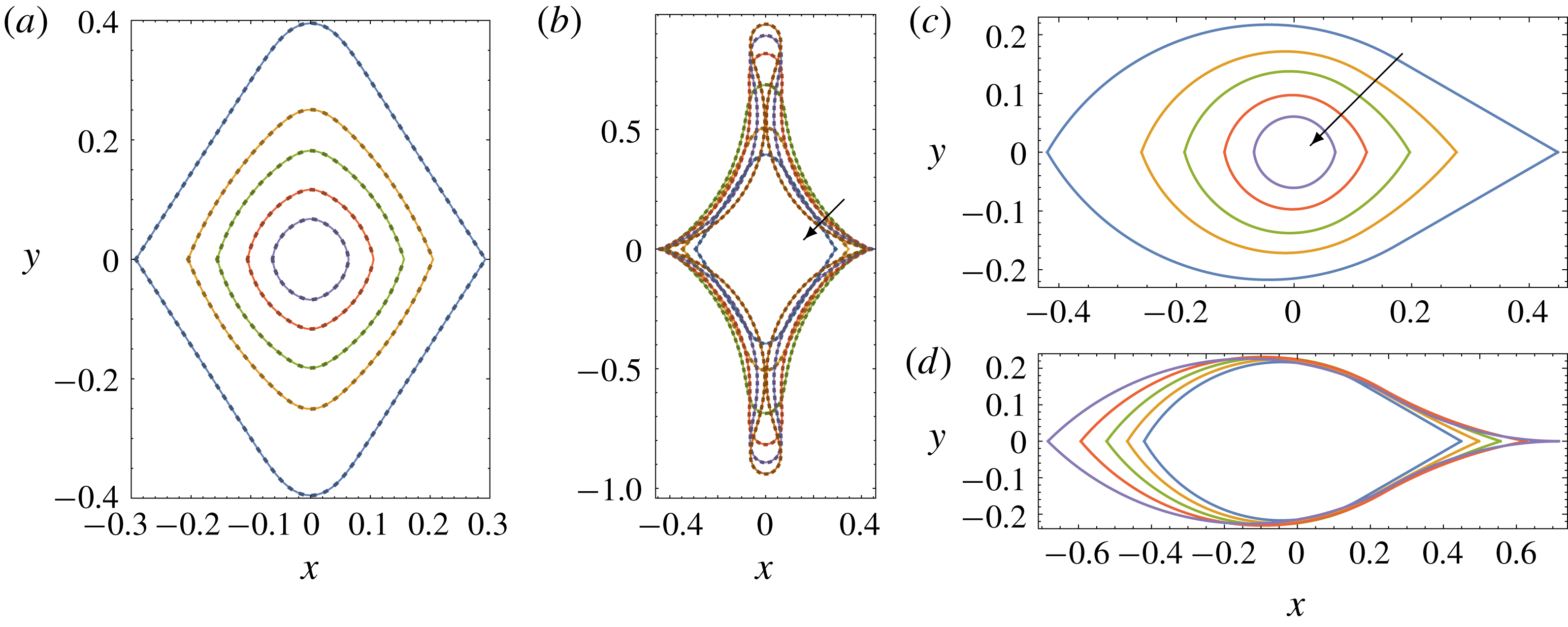
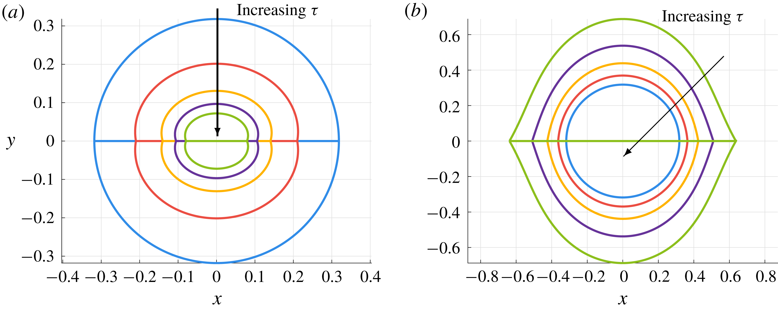
As demonstrated in figure 8(a,b), the reflectional symmetry is preserved, so that
 $\unicode[STIX]{x1D703}_{2}\equiv -\unicode[STIX]{x1D703}_{1}$
for all time. As
 $\unicode[STIX]{x1D70F}$
increases, the two-viscida system retracts under the action of surface tension and becomes increasingly circular, approaching the limiting solution (4.20) as expected. When the solution is calculated for negative time, the reverse happens, with each viscida becoming increasingly elongated and deformed, and a non-local self-intersection occurs when
 $\unicode[STIX]{x1D70F}\approx -1.16$
.
We note that the set-up shown in figure 7 may equivalently be viewed as a single closed-loop viscida containing two corners, rather than as a system of two viscidas whose ends are joined. Moreover, the initial condition (4.21) corresponds to a viscida centreline that is symmetric under rotation through
 $\unicode[STIX]{x03C0}$
. As shown by Griffiths & Howell (Reference Griffiths and Howell2007), this rotational invariance implies that the two tensions
 $A_{1}(\unicode[STIX]{x1D70F})$
and
 $B_{1}(\unicode[STIX]{x1D70F})$
must be identically zero, and we can therefore obtain the exact solution of the evolution equation (4.16) in this case, namely
 $$\begin{eqnarray}\unicode[STIX]{x1D703}_{1}(\unicode[STIX]{x1D709},\unicode[STIX]{x1D70F})=-\unicode[STIX]{x1D703}_{2}(\unicode[STIX]{x1D709},\unicode[STIX]{x1D70F})=\frac{\unicode[STIX]{x1D703}_{1}(\unicode[STIX]{x1D709},0)-\unicode[STIX]{x03C0}(1/2-\unicode[STIX]{x1D709})}{1+\unicode[STIX]{x1D70F}/2}+\unicode[STIX]{x03C0}(1/2-\unicode[STIX]{x1D709}).\end{eqnarray}$$
It is evident in figure 8(a,b) that our two-viscida solutions computed following the general approach described above agree essentially perfectly with the analytical solution (4.22), which is plotted using dotted curves.
Solutions of the system (4.16), (4.19) for two connected viscidas, plotted using Eulerian coordinates
 $(x,y)$
, with initial conditions given by (4.21) (a,b) and (4.23) (c,d). The times shown are (a)
 $\unicode[STIX]{x1D70F}\in \{0,1,2,4,8\}$
, (b)
 $\unicode[STIX]{x1D70F}\in \{-1.16,-1.1,-1.0,-0.8,-0.4,0\}$
, (c)
 $\unicode[STIX]{x1D70F}\in \{0,1,2,4,8\}$
, (d)
 $\unicode[STIX]{x1D70F}\in \{-2/3,-1/2,-1/3,-1/6,0\}$
, with the direction of increasing
 $\unicode[STIX]{x1D70F}$
indicated by an arrow in each panel. In (a,b), the dotted lines show the analytical result (4.22), which perfectly overlay the solid numerical curves.
Next we demonstrate our method on another two-viscida example, which has reflectional symmetry again, but not rotational symmetry. We impose the initial conditions
 $$\begin{eqnarray}\unicode[STIX]{x1D703}_{1}(\unicode[STIX]{x1D709},0)=-\unicode[STIX]{x1D703}_{2}(\unicode[STIX]{x1D709},0)=\left\{\begin{array}{@{}ll@{}}\displaystyle \frac{\unicode[STIX]{x03C0}}{3}-\left(\sqrt{3}+\frac{\unicode[STIX]{x03C0}}{2}-1\right)\unicode[STIX]{x1D709},\quad & \unicode[STIX]{x1D709}<{\displaystyle \frac{\unicode[STIX]{x03C0}}{2\sqrt{3}+\unicode[STIX]{x03C0}-2}},\\ \displaystyle -\frac{\unicode[STIX]{x03C0}}{6},\quad & \unicode[STIX]{x1D709}\geqslant {\displaystyle \frac{\unicode[STIX]{x03C0}}{2\sqrt{3}+\unicode[STIX]{x03C0}-2}},\end{array}\right.\end{eqnarray}$$
which describe a circular arc merged smoothly with a straight line, as can be seen in the ‘
 $t=0$
’ curves in figure 8(c,d). In this case, one can show that
 $A_{1}(\unicode[STIX]{x1D70F})$
is identically zero but
 $B_{1}(\unicode[STIX]{x1D70F})$
is strictly negative, so an analytical solution akin to (4.22) does not exist, and it is necessary to solve the system (4.16), (4.19) numerically.
The resulting solutions plotted in figure 8(c,d) again show the anticipated behaviour. As
 $\unicode[STIX]{x1D70F}$
increases, the corner angles increase towards
 $\unicode[STIX]{x03C0}$
and the system approaches a circular arc. As
 $\unicode[STIX]{x1D70F}$
decreases from zero, the corner angles sharpen, with a cusp forming at
 $\unicode[STIX]{x1D709}=1$
when
 $\unicode[STIX]{x1D70F}=-2/3$
, so that self-intersection would occur for
 $\unicode[STIX]{x1D70F}<-2/3$
.
4.2 A three-viscida network
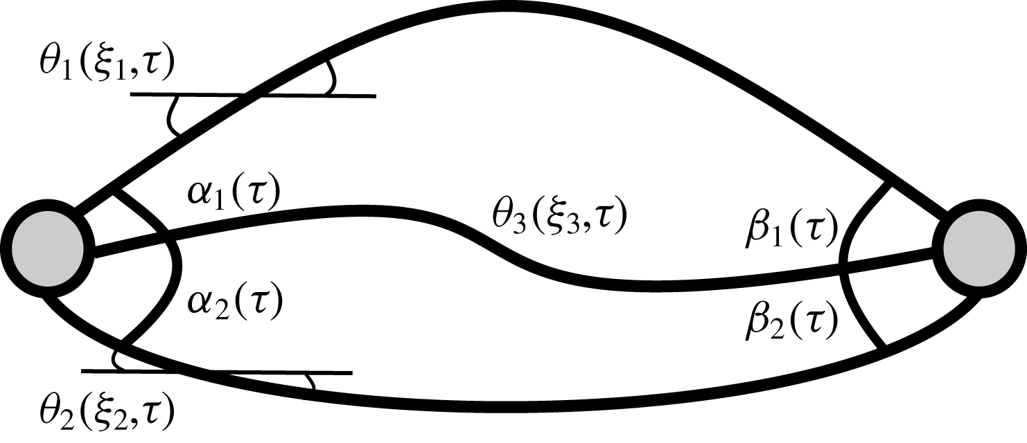
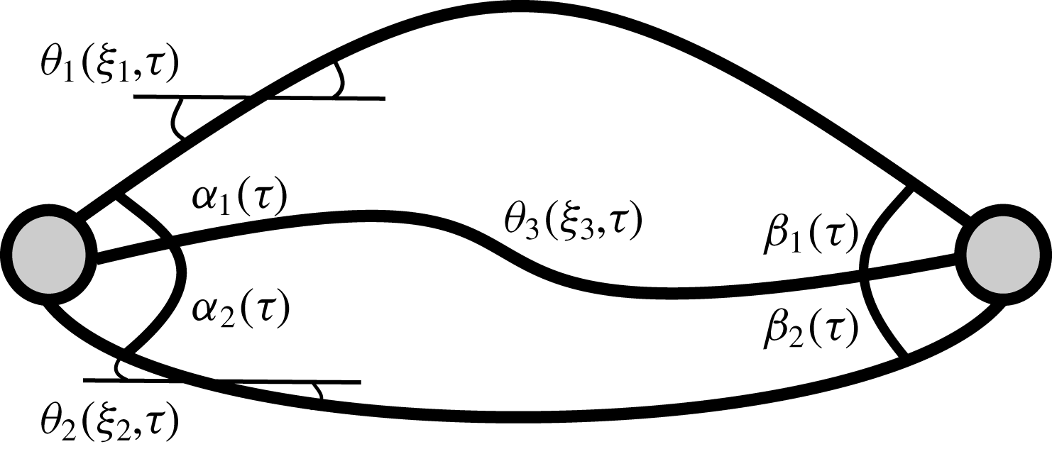
Next we analyse a network of three viscidas connected in the configuration illustrated in figure 9, with a three-way junction at either end. To describe such a situation, we must solve an evolution equation for each viscida, i.e.
 $$\begin{eqnarray}\frac{\unicode[STIX]{x2202}}{\unicode[STIX]{x2202}\unicode[STIX]{x1D70F}}\left[\left(1+\frac{\unicode[STIX]{x1D70F}}{2}\right)\frac{\unicode[STIX]{x2202}^{2}\unicode[STIX]{x1D703}_{i}}{\unicode[STIX]{x2202}\unicode[STIX]{x1D709}_{i}^{2}}\right]=A_{i}(\unicode[STIX]{x1D70F})\sin \unicode[STIX]{x1D703}_{i}+B_{i}(\unicode[STIX]{x1D70F})\cos \unicode[STIX]{x1D703}_{i},\end{eqnarray}$$
for
 $i\in \{1,2,3\}$
. We identify each spatial coordinate
 $\unicode[STIX]{x1D709}_{i}$
separately for clarity, since each viscida may have a different initial length, say
 $\ell _{i}$
. Twelve independent boundary conditions are required to solve for the three deflection angles
 $\unicode[STIX]{x1D703}_{i}(\unicode[STIX]{x1D709}_{i},\unicode[STIX]{x1D70F})$
and the six tensions
 $A_{i}(\unicode[STIX]{x1D70F})$
,
 $B_{i}(\unicode[STIX]{x1D70F})$
.
A system of three connected viscidas. The top, bottom and middle viscidas have centrelines described by
 $\unicode[STIX]{x1D703}_{1}(\unicode[STIX]{x1D709}_{1},\unicode[STIX]{x1D70F})$
,
 $\unicode[STIX]{x1D703}_{2}(\unicode[STIX]{x1D709}_{2},\unicode[STIX]{x1D70F})$
and
 $\unicode[STIX]{x1D703}_{3}(\unicode[STIX]{x1D709}_{3},\unicode[STIX]{x1D70F})$
, respectively. For
 $i\in \{1,2,3\}$
, the interior angles at
 $\unicode[STIX]{x1D709}_{i}=0$
are given by
 $\unicode[STIX]{x1D6FC}_{1,2}(\unicode[STIX]{x1D70F})$
, and the angles at
 $\unicode[STIX]{x1D709}_{i}=\ell _{i}$
are given by
 $\unicode[STIX]{x1D6FD}_{1,2}(\unicode[STIX]{x1D70F})$
. The two nodes represent the viscida junctions.
Since the ends must meet at the two junctions, we enforce
 $$\begin{eqnarray}\int _{0}^{\ell _{1}}\left(\begin{array}{@{}c@{}}\cos \unicode[STIX]{x1D703}_{1}\\ \sin \unicode[STIX]{x1D703}_{1}\end{array}\right)\,\text{d}\unicode[STIX]{x1D709}_{1}=\int _{0}^{\ell _{2}}\left(\begin{array}{@{}c@{}}\cos \unicode[STIX]{x1D703}_{2}\\ \sin \unicode[STIX]{x1D703}_{2}\end{array}\right)\,\text{d}\unicode[STIX]{x1D709}_{2}=\int _{0}^{\ell _{3}}\left(\begin{array}{@{}c@{}}\cos \unicode[STIX]{x1D703}_{3}\\ \sin \unicode[STIX]{x1D703}_{3}\end{array}\right)\text{d}\unicode[STIX]{x1D709}_{3}.\end{eqnarray}$$
The condition of zero net bending moment at each junction becomes, in this case,
 $$\begin{eqnarray}\frac{\unicode[STIX]{x2202}}{\unicode[STIX]{x2202}\unicode[STIX]{x1D70F}}\left[\left(1+\frac{\unicode[STIX]{x1D70F}}{2}\right)\left(\frac{\unicode[STIX]{x2202}\unicode[STIX]{x1D703}_{1}}{\unicode[STIX]{x2202}\unicode[STIX]{x1D709}_{1}}+\frac{\unicode[STIX]{x2202}\unicode[STIX]{x1D703}_{2}}{\unicode[STIX]{x2202}\unicode[STIX]{x1D709}_{2}}+\frac{\unicode[STIX]{x2202}\unicode[STIX]{x1D703}_{3}}{\unicode[STIX]{x2202}\unicode[STIX]{x1D709}_{3}}\right)\right]=0\quad \text{at }\unicode[STIX]{x1D709}_{j}=0,\ell _{j}\text{ for }j=1,2,3.\end{eqnarray}$$
Using (3.16) with
 $n=3$
, we write the evolution of the angles at the corners as
 $$\begin{eqnarray}\displaystyle & \displaystyle \unicode[STIX]{x1D6FC}_{i}(\unicode[STIX]{x1D70F})=\frac{2\unicode[STIX]{x03C0}}{3}+\frac{\unicode[STIX]{x1D6FC}_{i}(0)-2\unicode[STIX]{x03C0}/3}{1+\unicode[STIX]{x1D70F}/2}=(-1)^{i+1}[\unicode[STIX]{x1D703}_{i}(0,\unicode[STIX]{x1D70F})-\unicode[STIX]{x1D703}_{3}(0,\unicode[STIX]{x1D70F})], & \displaystyle\end{eqnarray}$$
 $$\begin{eqnarray}\displaystyle & \displaystyle \unicode[STIX]{x1D6FD}_{i}(\unicode[STIX]{x1D70F})=\frac{2\unicode[STIX]{x03C0}}{3}+\frac{\unicode[STIX]{x1D6FD}_{i}(0)-2\unicode[STIX]{x03C0}/3}{1+\unicode[STIX]{x1D70F}/2}=(-1)^{i+1}[\unicode[STIX]{x1D703}_{3}(\ell _{3},\unicode[STIX]{x1D70F})-\unicode[STIX]{x1D703}_{i}(\ell _{i},\unicode[STIX]{x1D70F})], & \displaystyle\end{eqnarray}$$
 $i\in \{1,2\}$
. Here
 $\unicode[STIX]{x1D6FC}_{1,2}(0)$
and
 $\unicode[STIX]{x1D6FD}_{1,2}(0)$
are the initial internal angles at each junction, as illustrated in figure 9. Force balances at
 $\unicode[STIX]{x1D709}_{i}=0,\ell _{i}$
for
 $i\in \{1,2,3\}$
imply that there must be zero resultant forces in the
 $x$
- and
 $y$
-directions, for all
 $\unicode[STIX]{x1D70F}$
, i.e.
 $$\begin{eqnarray}\mathop{\sum }_{i=1}^{3}A_{i}(\unicode[STIX]{x1D70F})=0\quad \text{and}\quad \mathop{\sum }_{i=1}^{3}B_{i}(\unicode[STIX]{x1D70F})=0.\end{eqnarray}$$
Equations (4.25)–(4.28) provide twelve boundary conditions for the system (4.24). However, as in § 4.1, the problem suffers from a rotational indeterminacy. By integrating the evolution equation (4.24) along the length of each viscida from
 $\unicode[STIX]{x1D709}_{i}=0$
to
 $\unicode[STIX]{x1D709}_{i}=\ell _{i}$
and applying the force balances (4.28), we see that the moment balance (4.26) is satisfied identically at
 $\unicode[STIX]{x1D709}_{i}=\ell _{i}$
if it is enforced at
 $\unicode[STIX]{x1D709}_{i}=0$
. Therefore one more condition must be imposed to determine all of the angles
 $\unicode[STIX]{x1D703}_{i}(\unicode[STIX]{x1D709}_{i},\unicode[STIX]{x1D70F})$
uniquely, and then a further two conditions are needed to fix the translation of the entire network. The details of the calculation to determine the evolution of the three-viscida network may be found in appendix A.
We illustrate the evolution of a three-viscida network with an initial configuration given by
 $$\begin{eqnarray}\displaystyle & \unicode[STIX]{x1D703}_{1}(\unicode[STIX]{x1D709}_{1},0)=\unicode[STIX]{x03C0}(1/2-\unicode[STIX]{x1D709}_{1}),\quad \text{for }0\leqslant \unicode[STIX]{x1D709}_{1}\leqslant 1, & \displaystyle\end{eqnarray}$$
 $$\begin{eqnarray}\displaystyle & \unicode[STIX]{x1D703}_{2}(\unicode[STIX]{x1D709}_{2},0)=\unicode[STIX]{x03C0}(\unicode[STIX]{x1D709}_{2}-1/2),\quad \text{for }0\leqslant \unicode[STIX]{x1D709}_{2}\leqslant 1, & \displaystyle\end{eqnarray}$$
 $$\begin{eqnarray}\displaystyle & \unicode[STIX]{x1D703}_{3}(\unicode[STIX]{x1D709}_{3},0)=0,\quad \text{for }0\leqslant \unicode[STIX]{x1D709}_{3}\leqslant 2/\unicode[STIX]{x03C0}, & \displaystyle\end{eqnarray}$$
For forward time, the internal angles formed at the junctions evolve towards
 $2\unicode[STIX]{x03C0}/3$
, while the outer viscidas want to approach circular arcs, but the specified (Lagrangian) lengths are incompatible with such a configuration. The system resolves this frustration by approaching two semi-circular arcs (similar to the initial condition), with the angle adjusting rapidly to satisfy the required angle conditions in boundary layers near the two junctions. The profile for negative time shows the cross-sectional profile that we should begin with to achieve a final circular tube cross-section with a central partitioning viscida.


4.3 A general viscida network model
We now combine the ideas presented so far to construct a general framework that describes the evolution of an arbitrary system of
 $N$
thin viscidas connected at
 $J$
junctions. In principle the resulting model can ultimately be used to describe the fabrication of a MOF.
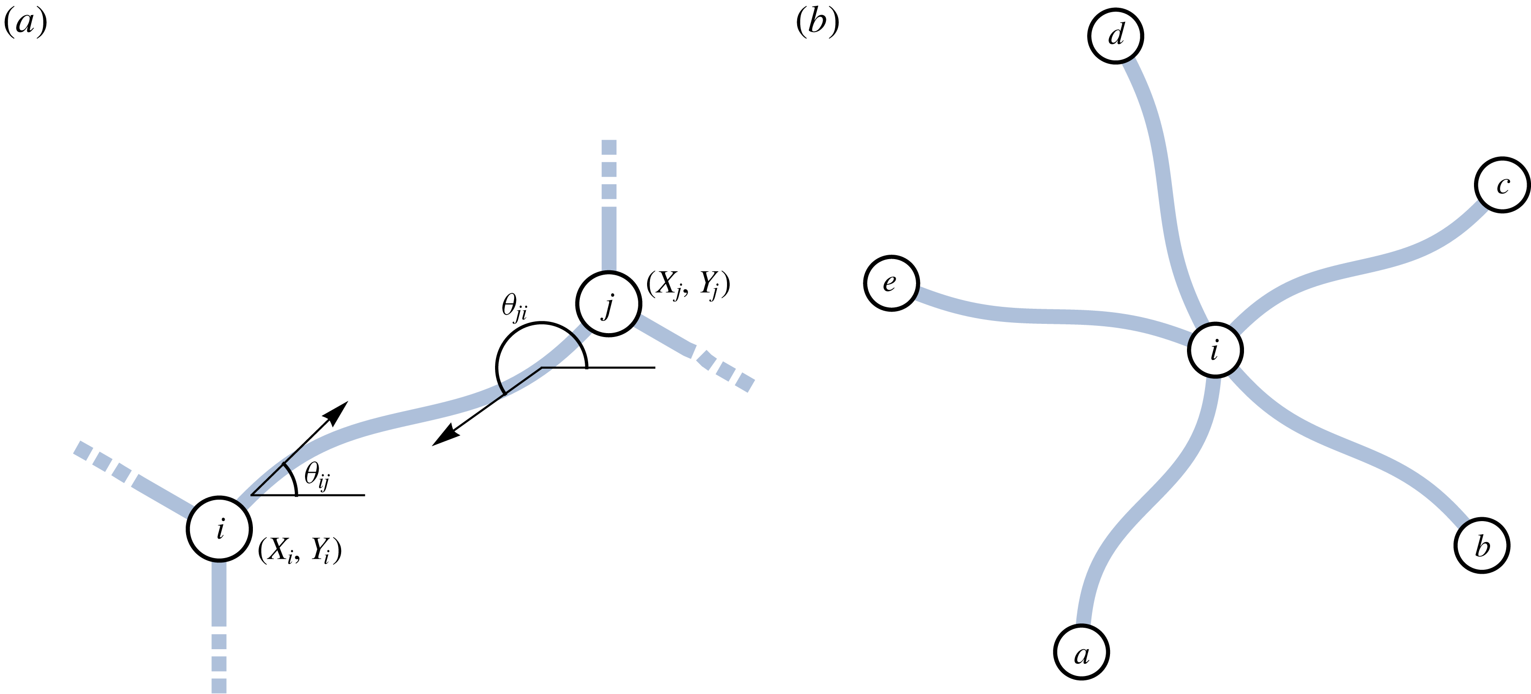
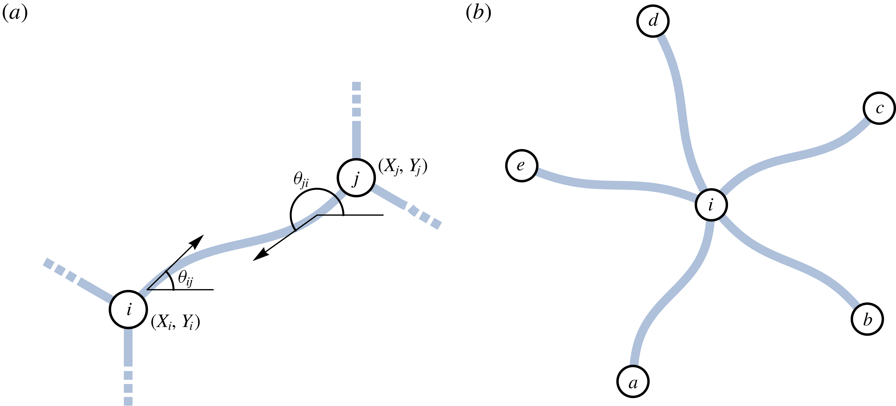
As shown schematically in figure 11(a), we describe the shape of a viscida that goes from junction
 $i$
to junction
 $j$
(with
 $1\leqslant i\neq j\leqslant J$
) by the inclination angle
 $\unicode[STIX]{x1D703}_{ij}(\unicode[STIX]{x1D709},\unicode[STIX]{x1D70F})$
. For each of the
 $N$
such viscidas, we have to solve a version of the evolution equation (4.1), i.e.
 $$\begin{eqnarray}\frac{\unicode[STIX]{x2202}}{\unicode[STIX]{x2202}\unicode[STIX]{x1D70F}}\left[\left(1+\frac{\unicode[STIX]{x1D70F}}{2}\right)\frac{\unicode[STIX]{x2202}^{2}\unicode[STIX]{x1D703}_{ij}}{\unicode[STIX]{x2202}\unicode[STIX]{x1D709}^{2}}\right]=A_{ij}(\unicode[STIX]{x1D70F})\sin \unicode[STIX]{x1D703}_{ij}+B_{ij}(\unicode[STIX]{x1D70F})\cos \unicode[STIX]{x1D703}_{ij},\end{eqnarray}$$
for
 $\unicode[STIX]{x1D709}\in (0,\ell _{ij})$
, where
 $\ell _{ij}$
is the viscida’s initial length and
 $(A_{ij},B_{ij})$
are the scaled tension components. Considering the same viscida instead as going from junction
 $j$
to junction
 $i$
, we deduce the symmetry conditions
 $$\begin{eqnarray}A_{ji}(\unicode[STIX]{x1D70F})\equiv -A_{ij}(\unicode[STIX]{x1D70F}),\quad B_{ji}(\unicode[STIX]{x1D70F})\equiv -B_{ij}(\unicode[STIX]{x1D70F}),\quad \ell _{ji}\equiv \ell _{ij},\end{eqnarray}$$
and
 $$\begin{eqnarray}\unicode[STIX]{x1D703}_{ji}(\unicode[STIX]{x1D709},\unicode[STIX]{x1D70F})\equiv \pm \unicode[STIX]{x03C0}+\unicode[STIX]{x1D703}_{ij}(\ell _{ij}-\unicode[STIX]{x1D709},\unicode[STIX]{x1D70F}).\end{eqnarray}$$
(a) Schematic of a viscida connecting two junctions labelled
 $i$
and
 $j$
. (b) A central junction
 $i$
connected to five others
 $\{a,b,c,d,e\}$
.
We note in passing that the set-up here appears to assume that there is only one viscida connecting each pair of junctions
 $(ij)$
and also that there are no viscidas that start and end at the same junction. Such cases can be dealt with either by introducing additional passive junctions (connecting two viscidas with interior angle
 $\unicode[STIX]{x03C0}$
) or by defining slightly more cumbersome notation, such as
 $\unicode[STIX]{x1D703}_{ij}^{k}$
, with the index
 $k$
enumerating all of the viscidas connecting junctions
 $i$
and
 $j$
. In either case, the arguments developed below follow through.
We denote the (anticlockwise) moment exerted on node
 $i$
by the viscida that connects it to node
 $j$
by
 $M_{ij}$
, which may be expressed in the form
 $$\begin{eqnarray}M_{ij}(\unicode[STIX]{x1D70F})=\left.\frac{\unicode[STIX]{x2202}}{\unicode[STIX]{x2202}\unicode[STIX]{x1D70F}}\left[(1+\unicode[STIX]{x1D70F}/2)\frac{\unicode[STIX]{x2202}\unicode[STIX]{x1D703}_{ij}}{\unicode[STIX]{x2202}\unicode[STIX]{x1D709}}\right]\right|_{\unicode[STIX]{x1D709}=0}.\end{eqnarray}$$
By integrating (4.30) between
 $\unicode[STIX]{x1D709}=0$
and
 $\unicode[STIX]{x1D709}=\ell _{ij}$
, and using the identity (4.32), we find a symmetry condition satisfied by
 $M_{ij}$
, namely
 $$\begin{eqnarray}M_{ij}(\unicode[STIX]{x1D70F})+M_{ji}(\unicode[STIX]{x1D70F})\equiv [X_{i}(\unicode[STIX]{x1D70F})-X_{j}(\unicode[STIX]{x1D70F})]\,B_{ij}(\unicode[STIX]{x1D70F})+[Y_{i}(\unicode[STIX]{x1D70F})-Y_{j}(\unicode[STIX]{x1D70F})]\,A_{ij}(\unicode[STIX]{x1D70F}),\end{eqnarray}$$
where
 $(X_{i},Y_{i})$
and
 $(X_{j},Y_{j})$
denote the positions of junction
 $i$
and junction
 $j$
, respectively.
Now, to impose the corner-evolution equation (3.16), we need to define the relevant interior angles between adjacent viscidas. To this end, let
 $v_{i}$
be an ordered list, enumerating the indices
 $j$
of the other junctions which are connected to junction
 $i$
, sorted in order of increasing
 $\unicode[STIX]{x1D703}_{ij}(0,0)$
; for example, in the scenario sketched in figure 11(b), we could take
 $v_{i}=\{a,b,c,d,e\}.$
Then the total number of viscidas connected at junction
 $i$
is
 $n_{i}=|v_{i}|$
, and the total number of viscidas in the network is
 $$\begin{eqnarray}N=\frac{1}{2}\mathop{\sum }_{i=1}^{J}n_{i}.\end{eqnarray}$$
It is also clear that
 $j\in v_{i}$
if and only if
 $i\in v_{j}$
.
We can now write the interior angles in terms of the differences between the angles corresponding to successive terms in the ordered list
 $v_{i}$
, i.e.
 $$\begin{eqnarray}\unicode[STIX]{x1D711}_{ik}(\unicode[STIX]{x1D70F})=\unicode[STIX]{x1D703}_{iv_{i}(k+1)}(0,\unicode[STIX]{x1D70F})-\unicode[STIX]{x1D703}_{iv_{i}(k)}(0,\unicode[STIX]{x1D70F}),\end{eqnarray}$$
where
 $v_{i}(k)$
denotes the
 $k$
th element in
 $v_{i}$
. Finally, applying the corner rule (3.16), we deduce that the angle with which each viscida leaves junction
 $i$
is given by
 $$\begin{eqnarray}\unicode[STIX]{x1D703}_{iv_{i}(k)}(0,\unicode[STIX]{x1D70F})=\unicode[STIX]{x1D6E9}_{i}(\unicode[STIX]{x1D70F})+\frac{\unicode[STIX]{x1D703}_{iv_{i}(k)}(0,0)}{1+\unicode[STIX]{x1D70F}/2}+\frac{(k-1)\unicode[STIX]{x03C0}\unicode[STIX]{x1D70F}}{n_{i}(1+\unicode[STIX]{x1D70F}/2)},\end{eqnarray}$$
where
 $\unicode[STIX]{x1D6E9}_{i}$
is an arbitrary function of
 $\unicode[STIX]{x1D70F}$
, which measures the net rotation of junction
 $i$
.
Let us suppose for a moment that we know the position
 $(X_{i}(\unicode[STIX]{x1D70F}),Y_{i}(\unicode[STIX]{x1D70F}))$
and rotation
 $\unicode[STIX]{x1D6E9}_{i}(\unicode[STIX]{x1D70F})$
of every junction
 $i=1,2,\ldots ,J$
. If so, then (4.37) determines the angle
 $\unicode[STIX]{x1D703}_{ij}$
at both ends of each viscida. In addition, the displacement between each pair of connected junctions is given by
 $$\begin{eqnarray}\int _{0}^{\ell _{ij}}\cos \unicode[STIX]{x1D703}_{ij}(\unicode[STIX]{x1D709},\unicode[STIX]{x1D70F})\,\text{d}\unicode[STIX]{x1D709}=X_{j}(\unicode[STIX]{x1D70F})-X_{i}(\unicode[STIX]{x1D70F}),\quad \int _{0}^{\ell _{ij}}\sin \unicode[STIX]{x1D703}_{ij}(\unicode[STIX]{x1D709},\unicode[STIX]{x1D70F})\,\text{d}\unicode[STIX]{x1D709}=Y_{j}(\unicode[STIX]{x1D70F})-Y_{i}(\unicode[STIX]{x1D70F}).\end{eqnarray}$$
In total, then, for each pair
 $(ij)$
with
 $j\in v_{i}$
, we have the four boundary conditions required to solve the evolution equation (4.30) uniquely for
 $A_{ij}(\unicode[STIX]{x1D70F})$
,
 $B_{ij}(\unicode[STIX]{x1D70F})$
and
 $\unicode[STIX]{x1D703}_{ij}(\unicode[STIX]{x1D709},\unicode[STIX]{x1D70F})$
.
Assuming we have solved for
 $\unicode[STIX]{x1D703}_{ij}(\unicode[STIX]{x1D709},\unicode[STIX]{x1D70F})$
, we can then evaluate all of the moments acting at each junction using (4.33). Finally, we impose force and moment balances at each junction, namely
 $$\begin{eqnarray}\mathop{\sum }_{j\in v_{i}}A_{ij}=\mathop{\sum }_{j\in v_{i}}B_{ij}=\mathop{\sum }_{j\in v_{i}}M_{ij}=0,\end{eqnarray}$$
for every
 $i=1,2,\ldots ,J$
. On the face of it, equation (4.39) provides the
 $3J$
equations required to determine the remaining unknowns
 $X_{i}$
,
 $Y_{i}$
and
 $\unicode[STIX]{x1D6E9}_{i}$
which we had temporarily imagined to be given. However, the problem suffers from a by now familiar degeneracy. By virtue of the symmetry conditions (4.31) and (4.34), it is easily shown that
 $$\begin{eqnarray}\mathop{\sum }_{i,j}A_{ij}\equiv \mathop{\sum }_{i,j}B_{ij}\equiv \mathop{\sum }_{i,j}M_{ij}\equiv 0,\end{eqnarray}$$
and therefore (4.39) actually provides only
 $3J-3$
independent equations, and there remain three degrees of freedom in the problem. To determine the solution uniquely, it is necessary to eliminate the arbitrary rigid-body motion, for example by fixing the position and rotation of a specific junction, say
 $X_{1}(\unicode[STIX]{x1D70F})=Y_{1}(\unicode[STIX]{x1D70F})=\unicode[STIX]{x1D6E9}_{1}(\unicode[STIX]{x1D70F})=0$
for all
 $\unicode[STIX]{x1D70F}$
.
We thus argue that the system of equations, boundary conditions and balance laws developed above results in a well-posed evolution problem for the shape of each viscida and the position and rotation of each junction. A general solution strategy is sketched out in appendix B.
We illustrate the general approach by solving for the evolution of a six-viscida tri-junction network, similar to the one shown in figure 3(b). We prescribe the initial configuration
 $$\begin{eqnarray}\unicode[STIX]{x1D703}_{23}(\unicode[STIX]{x1D709},0)=\frac{2\unicode[STIX]{x03C0}}{3}\unicode[STIX]{x1D709},\quad \unicode[STIX]{x1D703}_{34}(\unicode[STIX]{x1D709},0)=\frac{2\unicode[STIX]{x03C0}}{3}(\unicode[STIX]{x1D709}+1),\quad \unicode[STIX]{x1D703}_{42}(\unicode[STIX]{x1D709},0)=\frac{2\unicode[STIX]{x03C0}}{3}(\unicode[STIX]{x1D709}+2),\end{eqnarray}$$
for
 $0\leqslant \unicode[STIX]{x1D709}\leqslant 1$
, and
 $$\begin{eqnarray}\unicode[STIX]{x1D703}_{13}(\unicode[STIX]{x1D709},0)=\frac{\unicode[STIX]{x03C0}}{6},\quad \unicode[STIX]{x1D703}_{14}(\unicode[STIX]{x1D709},0)=\frac{5\unicode[STIX]{x03C0}}{6},\quad \unicode[STIX]{x1D703}_{15}(\unicode[STIX]{x1D709},0)=\frac{9\unicode[STIX]{x03C0}}{6},\end{eqnarray}$$
for
 $0\leqslant \unicode[STIX]{x1D709}\leqslant 3/2\unicode[STIX]{x03C0}$
, impose the angle-evolution equation (3.16) at each junction, and ensure that the ends join up by setting
 $$\begin{eqnarray}\displaystyle & (x_{13}(3/2\unicode[STIX]{x03C0},\unicode[STIX]{x1D70F}),y_{13}(3/2\unicode[STIX]{x03C0},\unicode[STIX]{x1D70F}))=(x_{23}(1,\unicode[STIX]{x1D70F}),y_{23}(1,\unicode[STIX]{x1D70F}))=(x_{34}(0,\unicode[STIX]{x1D70F}),y_{34}(0,\unicode[STIX]{x1D70F})),\qquad & \displaystyle\end{eqnarray}$$
 $$\begin{eqnarray}\displaystyle & (x_{14}(3/2\unicode[STIX]{x03C0},\unicode[STIX]{x1D70F}),y_{14}(3/2\unicode[STIX]{x03C0},\unicode[STIX]{x1D70F}))=(x_{34}(1,\unicode[STIX]{x1D70F}),y_{34}(1,\unicode[STIX]{x1D70F}))=(x_{42}(1,\unicode[STIX]{x1D70F}),y_{42}(1,\unicode[STIX]{x1D70F})),\qquad & \displaystyle\end{eqnarray}$$
 $$\begin{eqnarray}\displaystyle & (x_{12}(3/2\unicode[STIX]{x03C0},\unicode[STIX]{x1D70F}),y_{12}(3/2\unicode[STIX]{x03C0},\unicode[STIX]{x1D70F}))=(x_{42}(1,\unicode[STIX]{x1D70F}),y_{42}(1,\unicode[STIX]{x1D70F}))=(x_{23}(0,\unicode[STIX]{x1D70F}),y_{23}(0,\unicode[STIX]{x1D70F})),\qquad & \displaystyle\end{eqnarray}$$
 $$\begin{eqnarray}\displaystyle & (x_{12}(0,\unicode[STIX]{x1D70F}),y_{12}(0,\unicode[STIX]{x1D70F}))=(x_{13}(0,\unicode[STIX]{x1D70F}),y_{13}(0,\unicode[STIX]{x1D70F}))=(x_{14}(0,\unicode[STIX]{x1D70F}),y_{14}(0,\unicode[STIX]{x1D70F})).\qquad & \displaystyle\end{eqnarray}$$
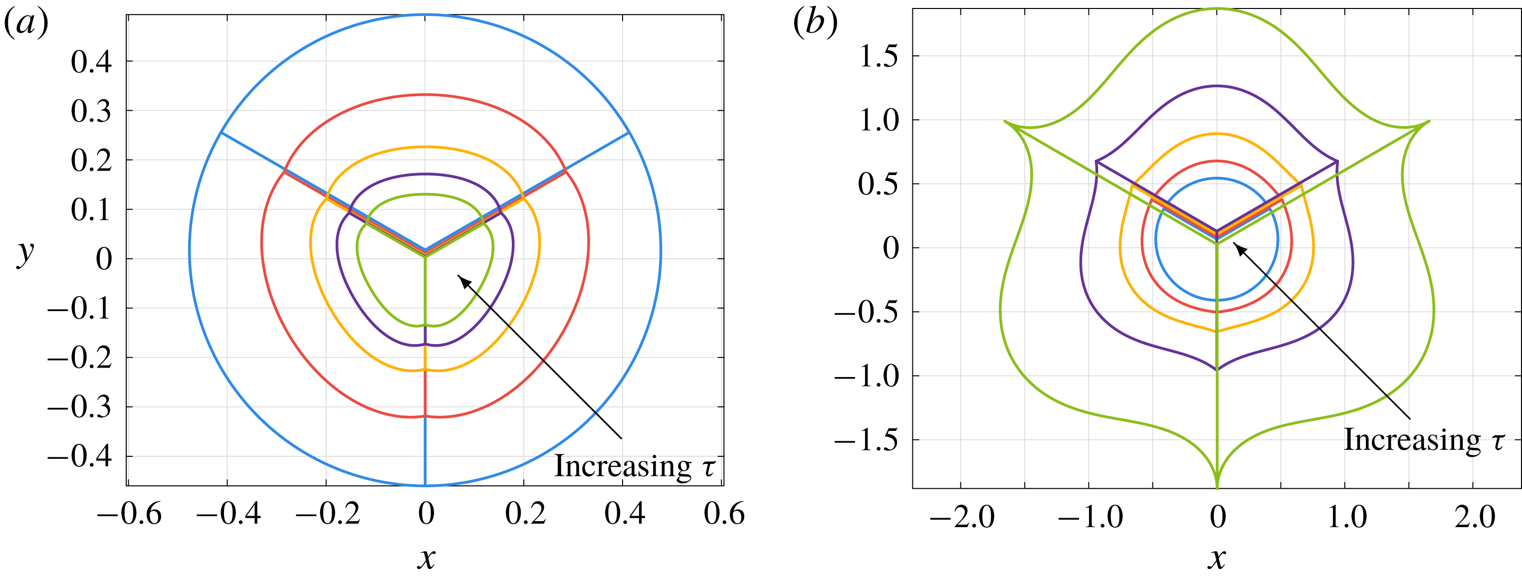
We show the evolution of such a profile for both forward and inverse time in figure 12. The rotational symmetry of the initial condition (4.41) is preserved by the dynamics, so the central struts remain straight and the interior angles at the centre remain equal to
 $2\unicode[STIX]{x03C0}/3$
for all time. The junctions at the edge become more symmetric as
 $\unicode[STIX]{x1D70F}$
increases, with all of the interior angles approaching
 $2\unicode[STIX]{x03C0}/3$
, but become increasingly asymmetric as
 $\unicode[STIX]{x1D70F}$
becomes increasingly negative. In either case, the evolution of the angles at the junctions imposes forces and moments on the curved viscidas and causes them to lose their initially circular shapes. At
 $\unicode[STIX]{x1D70F}=-3/2$
, the angles between the radial struts and the curved viscidas become zero, leading to self-intersection for
 $\unicode[STIX]{x1D70F}<-3/2$
.



5 Effects of varying thickness
5.1 Viscida evolution
Thus far in this paper, we have studied systems of thin viscidas that are joined together in a variety of configurations, to capture the complex network structure of the cross-section of a microstructured optical fibre. However, so far we have assumed throughout that every viscida in our network structure has equal and uniform thickness. In this section we return to the full equation of motion (2.9) to study the dynamics of a viscida with non-uniform initial thickness profile
 $h_{0}(\unicode[STIX]{x1D709})$
. In many of the real-life examples shown in figure 3, the connecting struts do not have uniform thickness. In particular, the honeycomb structure of figure 3(d) has struts that thicken as they approach junctions.
To explore the possible effects of thickness variations on the dynamics, we first consider the example of a single viscida with free ends at which no force or moment is applied. In this case, the evolution is governed by (2.9) with the tensions
 $A=B=0$
and zero-moment boundary conditions at the ends,
 $$\begin{eqnarray}\frac{\unicode[STIX]{x2202}}{\unicode[STIX]{x2202}\unicode[STIX]{x1D70F}}\left[\frac{h_{0}(\unicode[STIX]{x1D709})+\unicode[STIX]{x1D70F}/2}{h_{0}(\unicode[STIX]{x1D709})}\frac{\unicode[STIX]{x2202}\unicode[STIX]{x1D703}}{\unicode[STIX]{x2202}\unicode[STIX]{x1D709}}\right]=0\quad \text{at }\unicode[STIX]{x1D709}=0,1.\end{eqnarray}$$
We can therefore integrate (2.9) directly with respect to
 $\unicode[STIX]{x1D709}$
and
 $\unicode[STIX]{x1D70F}$
, subject to a specified initial centreline profile
 $\unicode[STIX]{x1D703}(\unicode[STIX]{x1D709},0)=\unicode[STIX]{x1D703}_{0}(\unicode[STIX]{x1D709})$
to give
 $$\begin{eqnarray}\unicode[STIX]{x1D703}(\unicode[STIX]{x1D709},\unicode[STIX]{x1D70F})=D(\unicode[STIX]{x1D70F})+\int _{0}^{\unicode[STIX]{x1D709}}\frac{h_{0}(\hat{\unicode[STIX]{x1D709}})}{h_{0}(\hat{\unicode[STIX]{x1D709}})+\unicode[STIX]{x1D70F}/2}\unicode[STIX]{x1D703}_{0}^{\prime }(\hat{\unicode[STIX]{x1D709}})\,\text{d}\hat{\unicode[STIX]{x1D709}},\end{eqnarray}$$
where
 $D(\unicode[STIX]{x1D70F})$
is an integration function. Two further integrations are required to evaluate the centreline profile, which is given by
 $$\begin{eqnarray}\displaystyle & \displaystyle x(\unicode[STIX]{x1D709},\unicode[STIX]{x1D70F})=x(0,\unicode[STIX]{x1D70F})+\int _{0}^{\unicode[STIX]{x1D709}}\frac{h_{0}(\hat{\unicode[STIX]{x1D709}})\cos \unicode[STIX]{x1D703}(\hat{\unicode[STIX]{x1D709}},\unicode[STIX]{x1D70F})}{h_{0}(\hat{\unicode[STIX]{x1D709}})+\unicode[STIX]{x1D70F}/2}\,\text{d}\hat{\unicode[STIX]{x1D709}}, & \displaystyle\end{eqnarray}$$
 $$\begin{eqnarray}\displaystyle & \displaystyle y(\unicode[STIX]{x1D709},\unicode[STIX]{x1D70F})=y(0,\unicode[STIX]{x1D70F})+\int _{0}^{\unicode[STIX]{x1D709}}\frac{h_{0}(\hat{\unicode[STIX]{x1D709}})\sin \unicode[STIX]{x1D703}(\hat{\unicode[STIX]{x1D709}},\unicode[STIX]{x1D70F})}{h_{0}(\hat{\unicode[STIX]{x1D709}})+\unicode[STIX]{x1D70F}/2}\,\text{d}\hat{\unicode[STIX]{x1D709}}. & \displaystyle\end{eqnarray}$$
 $D(\unicode[STIX]{x1D70F})$
,
 $x(0,\unicode[STIX]{x1D70F})$
and
 $y(0,\unicode[STIX]{x1D70F})$
, which correspond to rigid-body translations and rotations, by fixing the positions of the ends according to
 $$\begin{eqnarray}x(0,\unicode[STIX]{x1D70F})+\int _{0}^{1}\frac{(1-\unicode[STIX]{x1D709})h_{0}(\unicode[STIX]{x1D709})\cos \unicode[STIX]{x1D703}(\unicode[STIX]{x1D709},\unicode[STIX]{x1D70F})}{h_{0}(\unicode[STIX]{x1D709})+\unicode[STIX]{x1D70F}/2}\,\text{d}\unicode[STIX]{x1D709}=y(0,\unicode[STIX]{x1D70F})=y(1,\unicode[STIX]{x1D70F})=0.\end{eqnarray}$$
This choice results in the viscida having both ends lying on the
 $x$
-axis and the centroid at
 $x=0$
.
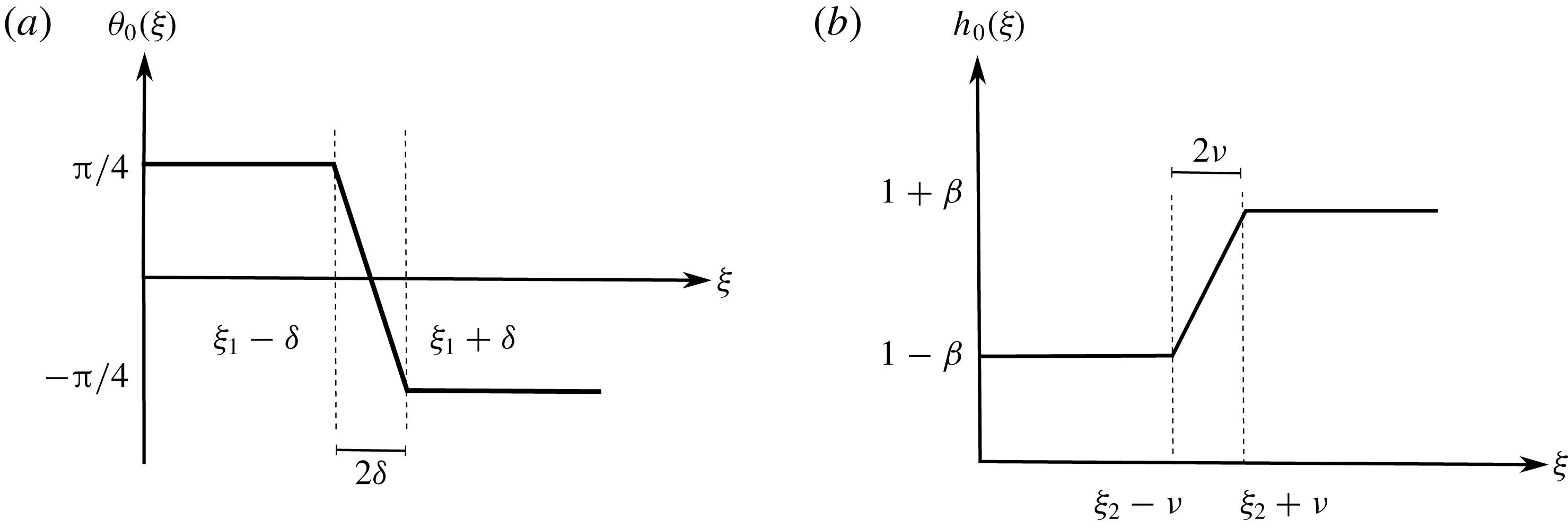
We calculate the solutions given by (5.2) and (5.3) for a free viscida with specific initial centreline and thickness configurations, given respectively by
 $$\begin{eqnarray}\unicode[STIX]{x1D703}_{0}(\unicode[STIX]{x1D709})=\left\{\begin{array}{@{}ll@{}}\displaystyle \frac{\unicode[STIX]{x03C0}}{4},\quad & 0\leqslant \unicode[STIX]{x1D709}\leqslant \unicode[STIX]{x1D709}_{1}-\unicode[STIX]{x1D6FF},\\ \displaystyle \frac{\unicode[STIX]{x03C0}}{4}\left(\frac{\unicode[STIX]{x1D709}_{1}-\unicode[STIX]{x1D709}}{\unicode[STIX]{x1D6FF}}\right),\quad & \unicode[STIX]{x1D709}_{1}-\unicode[STIX]{x1D6FF}<\unicode[STIX]{x1D709}<\unicode[STIX]{x1D709}_{1}+\unicode[STIX]{x1D6FF},\\ -\displaystyle \frac{\unicode[STIX]{x03C0}}{4},\quad & \unicode[STIX]{x1D709}_{1}+\unicode[STIX]{x1D6FF}\leqslant \unicode[STIX]{x1D709}\leqslant 1,\end{array}\right.\end{eqnarray}$$
and
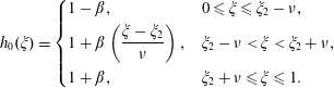 $$\begin{eqnarray}h_{0}(\unicode[STIX]{x1D709})=\left\{\begin{array}{@{}ll@{}}1-\unicode[STIX]{x1D6FD},\quad & 0\leqslant \unicode[STIX]{x1D709}\leqslant \unicode[STIX]{x1D709}_{2}-\unicode[STIX]{x1D708},\\ 1+\unicode[STIX]{x1D6FD}\displaystyle \left(\frac{\unicode[STIX]{x1D709}-\unicode[STIX]{x1D709}_{2}}{\unicode[STIX]{x1D708}}\right),\quad & \unicode[STIX]{x1D709}_{2}-\unicode[STIX]{x1D708}<\unicode[STIX]{x1D709}<\unicode[STIX]{x1D709}_{2}+\unicode[STIX]{x1D708},\\ 1+\unicode[STIX]{x1D6FD},\quad & \unicode[STIX]{x1D709}_{2}+\unicode[STIX]{x1D708}\leqslant \unicode[STIX]{x1D709}\leqslant 1.\end{array}\right.\end{eqnarray}$$
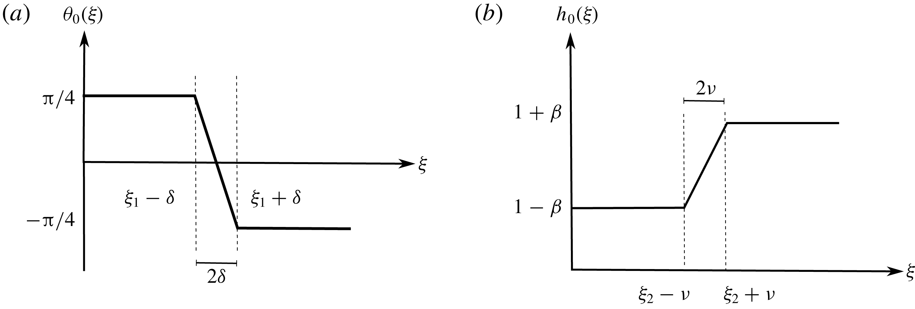
This formulation corresponds to an initial viscida whose angle transitions linearly from
 $\unicode[STIX]{x03C0}/4$
to
 $-\unicode[STIX]{x03C0}/4$
over a region of width
 $2\unicode[STIX]{x1D6FF}$
centred at
 $\unicode[STIX]{x1D709}=\unicode[STIX]{x1D709}_{1}$
and whose thickness varies linearly from
 $1-\unicode[STIX]{x1D6FD}$
to
 $1+\unicode[STIX]{x1D6FD}$
over a region of width
 $2\unicode[STIX]{x1D708}$
centred at
 $\unicode[STIX]{x1D709}=\unicode[STIX]{x1D709}_{2}$
. The functions defined by (5.5) and (5.6) are sketched in figure 13. We will take small values of
 $\unicode[STIX]{x1D6FF}$
and
 $\unicode[STIX]{x1D708}$
so that the transitions in both angle and thickness are localized.
Evolution of the centreline for a free viscida whose initial angle and thickness profiles are given by (5.5) and (5.6), with
 $\unicode[STIX]{x1D6FD}=0.3$
and
 $\unicode[STIX]{x1D709}_{1}=\unicode[STIX]{x1D709}_{2}=1/2$
. (a) We fix
 $\unicode[STIX]{x1D708}=0$
and vary
 $\unicode[STIX]{x1D6FF}\in \{0.01,0.08,0.15\}$
(dotted, dot-dashed and solid lines). (b) We fix
 $\unicode[STIX]{x1D6FF}=0$
and vary
 $\unicode[STIX]{x1D708}\in \{0.1,0.3,0.5\}$
.
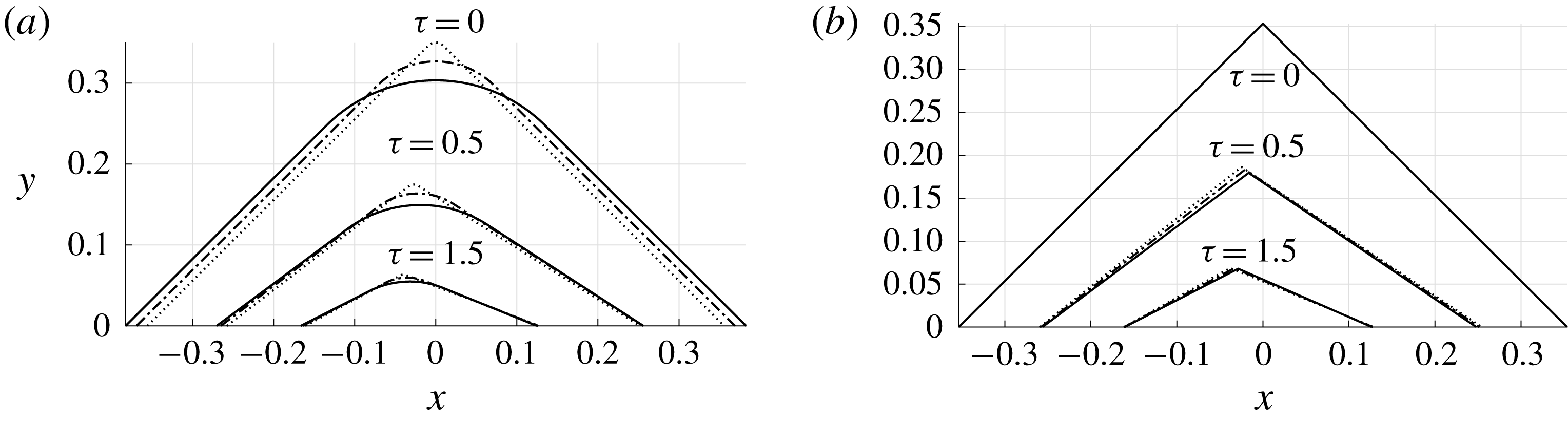
In figure 14 we plot solutions for the evolution of a free viscida, as given by (5.2)–(5.4), for an initial angle and thickness profile given by (5.5) and (5.6). We choose
 $\unicode[STIX]{x1D709}_{1}=\unicode[STIX]{x1D709}_{2}=1/2$
so that the transitions in angle and thickness both occur close to the central point of the viscida.
In figure 14(a), we set
 $\unicode[STIX]{x1D708}=0$
, so that the thickness increases abruptly across
 $\unicode[STIX]{x1D709}=1/2$
, and then gradually decrease the angle smoothing parameter
 $\unicode[STIX]{x1D6FF}$
. As the viscida evolves, we observe that the effect of smoothing the angle remains localized near
 $\unicode[STIX]{x1D709}=1/2$
, and the solution appears to approach a well-defined limiting profile containing a corner as
 $\unicode[STIX]{x1D6FF}\rightarrow 0$
. These observations echo the behaviour found for a uniformly thick viscida by Griffiths & Howell (Reference Griffiths and Howell2007). The thickness variations lead to a loss of symmetry in the centreline profile as
 $\unicode[STIX]{x1D70F}$
increases, caused by the more rapid retraction of the thinner region under the action of surface tension.
In figure 14(b), we perform the complementary experiment of setting
 $\unicode[STIX]{x1D6FF}=0$
, so the profile contains a sharp corner at
 $\unicode[STIX]{x1D709}=1/2$
, while varying the value of
 $\unicode[STIX]{x1D708}$
. We find that the corner is again pulled towards the left-hand end by capillary retraction, but that the way in which the transition in thickness is smoothed has very little effect on the global viscida behaviour.
Next we explore the influence on the dynamics of the relative positioning of the transition in angle relative to the transition in thickness. We find that the effect is most prominent when the viscida ends are fixed in place, rather than being free. We therefore solve the full evolution equation (2.9) subject to the boundary conditions
 $$\begin{eqnarray}\unicode[STIX]{x1D703}(0,\unicode[STIX]{x1D70F})=\unicode[STIX]{x1D703}(0,0),\quad \unicode[STIX]{x1D703}(1,\unicode[STIX]{x1D70F})=\unicode[STIX]{x1D703}(1,0),\end{eqnarray}$$
 $$\begin{eqnarray}x(0,\unicode[STIX]{x1D70F})=0,\quad x(1,\unicode[STIX]{x1D70F})=x(1,0),\end{eqnarray}$$
 $$\begin{eqnarray}y(0,\unicode[STIX]{x1D70F})=0,\quad y(1,\unicode[STIX]{x1D70F})=0,\end{eqnarray}$$
corresponding to clamping the end points of the viscida at fixed angles at fixed locations on the
 $x$
-axis. For the details of the calculations to determine the resulting viscida evolution, see appendix C.
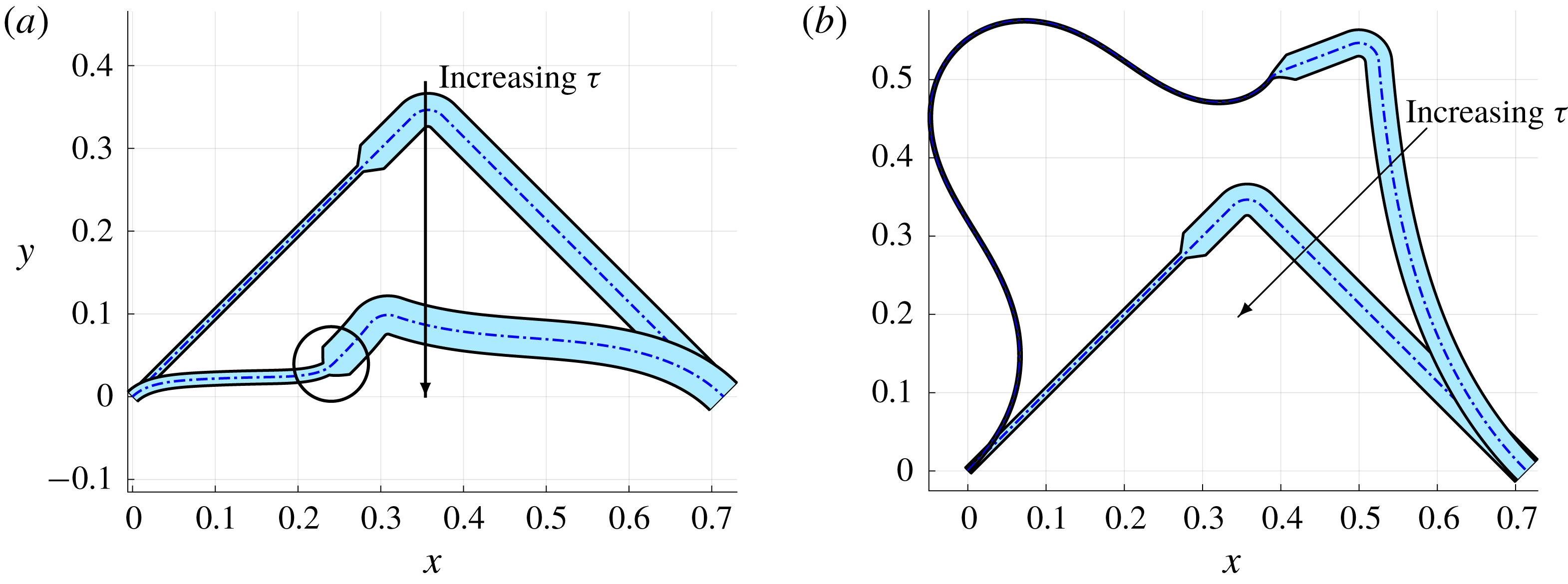
Evolution in Eulerian coordinates of a profile with rapid local angle and thickness variations at different locations along the viscida. The initial angle and thickness are given by (5.5) and (5.6) with parameter values
 $\unicode[STIX]{x1D6FF}=0.02$
,
 $\unicode[STIX]{x1D708}=0.01$
,
 $\unicode[STIX]{x1D6FD}=0.6$
,
 $\unicode[STIX]{x1D709}_{1}=1/2$
and
 $\unicode[STIX]{x1D709}_{2}=0.4$
. The dot-dashed line indicates the centreline and the shaded region depicts the viscida thickness. (a) The forward time evolution with
 $\unicode[STIX]{x1D70F}=0,0.5$
. (b) The inverse time evolution with
 $\unicode[STIX]{x1D70F}=-0.5,0$
. The circled region in (a) highlights the deflection generated with time at the thickness transition point.
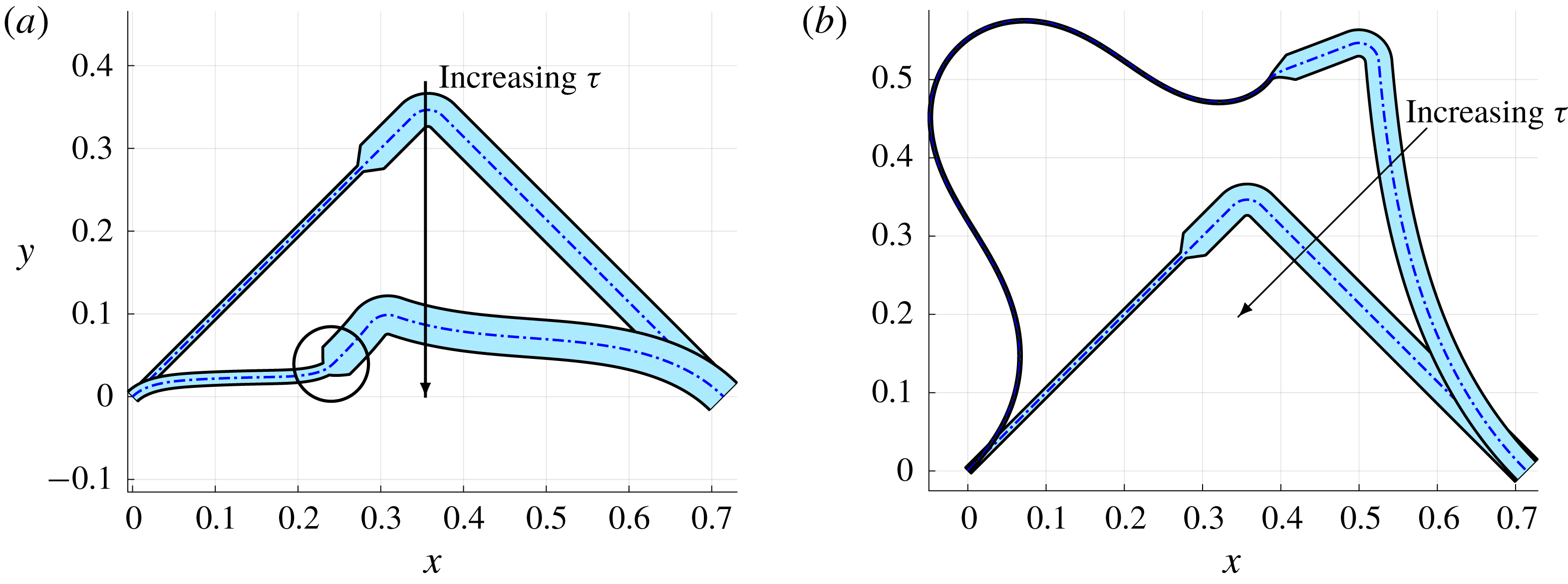
Figure 15 shows the evolution in both forward and inverse time of an initial profile with a smoothed corner at the central point
 $\unicode[STIX]{x1D709}=1/2$
and a sharp transition in thickness at a different location
 $\unicode[STIX]{x1D709}=0.4$
. As above we observe that the thinner section of the viscida retracts more rapidly as
 $\unicode[STIX]{x1D70F}$
increases, and it is also more susceptible to deformation. Since the effective bending stiffness is proportional to
 $h^{3}$
, the thicker portion of the viscida approximately preserves its shape, while the thinner portion undergoes significant bending. The effect is particularly marked in a neighbourhood of the thickness transition point, where the thinner section is effectively clamped by the thicker section. For inverse time, the thin part of the viscida rapidly becomes even thinner and longer while, again, being restrained by the thick part, which remains relatively unchanged. Consequently, the thin region adopts a profile akin to a buckled state (Buckmaster et al.
Reference Buckmaster, Nachman and Ting1975; Buckmaster & Nachman Reference Buckmaster and Nachman1978). In the manufacture of microstructured optical fibres, however, the original preform is usually constructed by sintering identical glass tubes, so it is unlikely that one would observe large variations in thickness.
5.2 A junction of two viscidas of different thicknesses
Figure 14 shows the evolution of several viscida profiles in which sharp changes in angle and thickness both occur at the same location. Here we consider in detail the limit as the smoothing parameters
 $\unicode[STIX]{x1D6FF}$
and
 $\unicode[STIX]{x1D708}$
both tend to zero, so that the limiting configuration describes a junction between two viscidas of differing thicknesses. As in § 3.1, we scale into the region over which the angle and thickness both vary rapidly via
 $\unicode[STIX]{x1D709}=\unicode[STIX]{x1D709}_{0}^{+}\unicode[STIX]{x1D6FF}\unicode[STIX]{x1D702}$
, and define
 $\unicode[STIX]{x1D6E9}(\unicode[STIX]{x1D702},\unicode[STIX]{x1D70F}):=\unicode[STIX]{x1D703}(\unicode[STIX]{x1D6FF}\unicode[STIX]{x1D702},\unicode[STIX]{x1D70F})$
and
 $H_{0}(\unicode[STIX]{x1D702}):=h_{0}(\unicode[STIX]{x1D6FF}\unicode[STIX]{x1D702})$
. We substitute these scalings into (2.9) and retain only leading-order terms in
 $\unicode[STIX]{x1D6FF}$
to obtain
 $$\begin{eqnarray}\frac{\unicode[STIX]{x2202}}{\unicode[STIX]{x2202}\unicode[STIX]{x1D702}}\left[(H_{0}(\unicode[STIX]{x1D702})+\unicode[STIX]{x1D70F}/2)^{3}\frac{\unicode[STIX]{x2202}}{\unicode[STIX]{x2202}\unicode[STIX]{x1D70F}}\left(\frac{H_{0}(\unicode[STIX]{x1D702})+\unicode[STIX]{x1D70F}/2}{H_{0}(\unicode[STIX]{x1D702})}\frac{\unicode[STIX]{x2202}\unicode[STIX]{x1D6E9}}{\unicode[STIX]{x2202}\unicode[STIX]{x1D702}}\right)\right]=0,\end{eqnarray}$$
which is subject to the initial condition
 $\unicode[STIX]{x1D6E9}(\unicode[STIX]{x1D702},0)=\unicode[STIX]{x1D6E9}_{0}(\unicode[STIX]{x1D702})$
and the matching conditions
 $\unicode[STIX]{x1D6E9}(\unicode[STIX]{x1D702},\unicode[STIX]{x1D70F})\rightarrow \unicode[STIX]{x1D703}(\unicode[STIX]{x1D709}_{0}^{\pm },\unicode[STIX]{x1D70F})$
as
 $\unicode[STIX]{x1D702}\rightarrow \pm \infty$
. By integrating (5.8), we obtain the following evolution law for the internal angle
 $\unicode[STIX]{x1D711}(\unicode[STIX]{x1D70F})=\unicode[STIX]{x03C0}+\unicode[STIX]{x1D703}(\unicode[STIX]{x1D709}_{0}^{-},\unicode[STIX]{x1D70F})-\unicode[STIX]{x1D703}(\unicode[STIX]{x1D709}_{0}^{+},\unicode[STIX]{x1D70F})$
:
 $$\begin{eqnarray}\displaystyle \unicode[STIX]{x03C0}-\unicode[STIX]{x1D711}(\unicode[STIX]{x1D70F}) & = & \displaystyle \int _{-\infty }^{\infty }\frac{H_{0}(\unicode[STIX]{x1D702})\unicode[STIX]{x1D6E9}_{0}^{\prime }(\unicode[STIX]{x1D702})}{H_{0}(\unicode[STIX]{x1D702})+\unicode[STIX]{x1D70F}/2}\,\text{d}\unicode[STIX]{x1D702}\end{eqnarray}$$
 $$\begin{eqnarray}\displaystyle & = & \displaystyle \frac{H_{+}\unicode[STIX]{x1D6E9}_{+}}{H_{+}+\unicode[STIX]{x1D70F}/2}-\frac{H_{-}\unicode[STIX]{x1D6E9}_{-}}{H_{-}+\unicode[STIX]{x1D70F}/2}-\frac{\unicode[STIX]{x1D70F}}{2}\int _{-\infty }^{\infty }\frac{H_{0}^{\prime }(\unicode[STIX]{x1D702})\unicode[STIX]{x1D6E9}_{0}(\unicode[STIX]{x1D702})}{(H_{0}(\unicode[STIX]{x1D702})+\unicode[STIX]{x1D70F}/2)^{2}}\,\text{d}\unicode[STIX]{x1D702},\end{eqnarray}$$
 $H_{\pm }=h_{0}(\unicode[STIX]{x1D709}_{0}^{\pm })=H_{0}(\pm \infty )$
and
 $\unicode[STIX]{x1D6E9}_{\pm }=\unicode[STIX]{x1D703}_{0}(\unicode[STIX]{x1D709}_{0}^{\pm })=\unicode[STIX]{x1D6E9}_{0}(\pm \infty )$
describe the initial jumps in thickness and angle at the junction. We note that (5.9) recovers the corner angle-evolution result (3.4) in the uniformly thick case
 $H_{0}(\unicode[STIX]{x1D702})=1$
. In a similar manner, we observe that the corner straightens in forward time, with
 $\unicode[STIX]{x1D711}\rightarrow \unicode[STIX]{x03C0}$
as
 $\unicode[STIX]{x1D70F}\rightarrow \infty$
, and becomes sharper for decreasing
 $\unicode[STIX]{x1D70F}$
, with
 $\unicode[STIX]{x1D711}$
reaching zero for some finite negative value of
 $\unicode[STIX]{x1D70F}$
, corresponding to self-intersection of the viscida.
In the case of a uniformly thick viscida, the corner evolution given by (3.4) depends only on the initial angle
 $\unicode[STIX]{x1D711}(0)$
and not on the precise way in which the initial angle profile
 $\unicode[STIX]{x1D6E9}_{0}(\unicode[STIX]{x1D702})$
varies from
 $\unicode[STIX]{x1D6E9}_{-}$
to
 $\unicode[STIX]{x1D6E9}_{+}$
. In contrast, equation (5.9) shows that, for a non-uniformly thick profile, the evolution of
 $\unicode[STIX]{x1D711}$
depends on the specific local behaviour of both the thickness profile
 $H_{0}(\unicode[STIX]{x1D702})$
and the angle variation
 $\unicode[STIX]{x1D6E9}_{0}(\unicode[STIX]{x1D702})$
. We illustrate this dependence by examining the two limiting cases where either the thickness variation occurs much more rapidly than the angle variation or vice versa.
The first limit corresponds to a viscida with a relatively slow change in angle around a smoothed corner, in the midst of which there is an abrupt jump in thickness, which we may take to occur at
 $\unicode[STIX]{x1D702}=0$
without loss of generality. In this case, the inner thickness profile
 $H_{0}(\unicode[STIX]{x1D702})$
collapses to a Heaviside function, and the angle-evolution equation (5.9) thus reduces to
 $$\begin{eqnarray}\unicode[STIX]{x03C0}-\unicode[STIX]{x1D711}(\unicode[STIX]{x1D70F})=\frac{H_{+}}{H_{+}+\unicode[STIX]{x1D70F}/2}(\unicode[STIX]{x1D6E9}_{+}-\unicode[STIX]{x1D6E9}_{0}(0))+\frac{H_{-}}{H_{-}+\unicode[STIX]{x1D70F}/2}(\unicode[STIX]{x1D6E9}_{0}(0)-\unicode[STIX]{x1D6E9}_{-}).\end{eqnarray}$$
We can interpret (5.10) as the sum of two evolution laws of the form (3.4) for the portions of the inner region in
 $\unicode[STIX]{x1D702}>0$
and
 $\unicode[STIX]{x1D702}<0$
, with effective initial thicknesses
 $H_{+}$
and
 $H_{-}$
, respectively.
In the reverse limit, the thickness varies relatively smoothly while the angle suddenly switches at a sharp corner at
 $\unicode[STIX]{x1D702}=0$
, so that
 $\unicode[STIX]{x1D6E9}_{0}(\unicode[STIX]{x1D702})$
may be replaced by a Heaviside function and (5.9) reduces to
 $$\begin{eqnarray}\unicode[STIX]{x03C0}-\unicode[STIX]{x1D711}(\unicode[STIX]{x1D70F})=\frac{H_{0}(0)}{H_{0}(0)+\unicode[STIX]{x1D70F}/2}(\unicode[STIX]{x03C0}-\unicode[STIX]{x1D711}(0)).\end{eqnarray}$$
Thus the uniform-thickness evolution law (3.4) is recovered in this case, with initial thickness effectively constant in the inner region, and equal to its value
 $H_{0}(0)$
at the corner.
Let us discuss the above results in the context of our piecewise linear example, with the initial angle and thickness given by (5.5) and (5.6), respectively. If
 $\unicode[STIX]{x1D709}_{1}=\unicode[STIX]{x1D709}_{2}$
, then the rapid variations in
 $\unicode[STIX]{x1D703}_{0}(\unicode[STIX]{x1D709})$
and
 $h_{0}(\unicode[STIX]{x1D709})$
are centred at the same point, as in the solutions plotted in figure 14, and the configuration approaches a junction between two viscidas of differing thicknesses as
 $\unicode[STIX]{x1D6FF}$
and
 $\unicode[STIX]{x1D708}$
both tend to zero. We have shown that the limiting behaviour depends on the order in which the limits
 $\unicode[STIX]{x1D6FF}\rightarrow 0$
and
 $\unicode[STIX]{x1D708}\rightarrow 0$
are taken: the interior angle satisfies (5.10) if
 $\unicode[STIX]{x1D708}\ll \unicode[STIX]{x1D6FF}\ll 1$
or (5.11) if
 $\unicode[STIX]{x1D6FF}\ll \unicode[STIX]{x1D708}\ll 1$
. In the distinguished limit where
 $\unicode[STIX]{x1D708}\sim \unicode[STIX]{x1D6FF}\ll 1$
, then the integrals in (5.9) must be computed, and the behaviour depends on the entire inner profiles of
 $\unicode[STIX]{x1D6E9}_{0}(\unicode[STIX]{x1D702})$
and
 $H_{0}(\unicode[STIX]{x1D702})$
.
As shown in § 3.1, a corner in a viscida with spatially uniform thickness may be analysed by regularizing the corner over a small length scale
 $\unicode[STIX]{x1D6FF}$
and then letting
 $\unicode[STIX]{x1D6FF}\rightarrow 0$
. The resulting limiting configuration also describes a junction between two viscidas of uniform and equal thickness, and the same approach also works when the thickness is non-uniform, provided it varies smoothly across the join. Of course, if
 $\unicode[STIX]{x1D6FF}$
becomes too small, then the asymptotic approximations used to derive the governing equations (2.1)–(2.3) cease to be valid. In principle one should then solve a two-dimensional inner Stokes-flow problem for the behaviour near the corner and match to the viscida model away from the corner. However, as argued by Griffiths & Howell (Reference Griffiths and Howell2007), the outer solution approaches a unique well-defined limit as
 $\unicode[STIX]{x1D6FF}\rightarrow 0$
, which does not depend on the behaviour in the inner region.
In this section we have found that the same regularization approach does not work for a junction where both the thickness and the angle vary rapidly. The introduction of a smoothing parameter
 $\unicode[STIX]{x1D6FF}$
does not result in a unique solution being selected as
 $\unicode[STIX]{x1D6FF}\rightarrow 0$
, and the evolution of the corner depends on the precise local behaviour of both
 $h$
and
 $\unicode[STIX]{x1D703}$
. A generalized moment-balance argument analogous to that in § 3.2 does not work either, since there is no well-defined interpretation of the product of distributions involved in the calculation of
 $M$
if both
 $h$
and
 $\unicode[STIX]{x1D703}$
are discontinuous. We conclude that the global behaviour of a junction between viscidas of different thicknesses ultimately depends on the solution in an inner region that is not described by the thin-viscida approximation, and there is no universal corner evolution law for such a configuration. To resolve the indeterminacy one would need to consider an inner Stokes-flow problem whose solution depends on precisely how the two viscidas are joined together.
6 Conclusions
In this paper we propose a new framework to describe the evolution of a network of thin viscidas, motivated by the drawing of microstructured optical fibres with closely spaced holes. We consider a parameter regime in which the dynamics is driven entirely by a balance between surface tension and viscosity. Similar network models used in foam dynamics (see for example Stewart, Davis & Hilgenfeldt Reference Stewart, Davis and Hilgenfeldt2015) operate in the regime where surface tension dominates, with the viscidas known as lamellae and the junctions as Plateau borders. In the case of foam dynamics, a difference in pressure across lamellae is also a key feature, which corresponds to the difference between the pressures in neighbouring bubbles. The modification of our model to include pressure in the governing equation (3.1), as described in Griffiths & Howell (Reference Griffiths and Howell2007), would make the set-up studied here more relevant to a foam.
Our approach allows a model to be built to describe a network of connected viscidas of arbitrary complexity. The numbers of partial differential equations of the form (4.30) and algebraic balance laws (4.31) to be solved grows linearly with the number of viscidas in the network, but the method of lines in principle leads to a manageable system of differential–algebraic equations, especially when any symmetries in the geometry are exploited. In comparison, numerical solution of the full two-dimensional Stokes-flow problem becomes increasingly onerous as the geometry of the viscous liquid inclusions between the air holes becomes increasingly thin and distorted.
Furthermore, the Stokes-flow free-boundary problem is ill posed when run backwards in time, but the viscida formulation remains well posed, because it filters out short-wavelength disturbances that grow arbitrarily quickly when time is run backwards. Thus our model provides an easy route to solve the inverse problem of determining the initial conditions that would evolve to a desired final state, as we demonstrate in several simple examples. The well posedness of the model for inverse time means that our theory can in principle provide the initial preform profile required to construct microstructured tubing with a desired final cross-section. The inclusion of internal pressurization in the model would add an extra level of control to the problem to open up the range of possible final cross-sectional profiles that can be constructed.
For viscidas of uniform thickness, time may be run backwards in our model up to the critical time
 $\unicode[STIX]{x1D70F}=-2$
, at which the thickness tends to zero and the viscida length tends to infinity. The solutions shown for example in figures 8 and 12 indicate that the viscida may self-intersect before this critical inverse time is reached. Indeed, the angle-evolution equation (3.16) implies that the interior angle
 $\unicode[STIX]{x1D711}_{i}(\unicode[STIX]{x1D70F})$
at a junction tends to zero as
 $\unicode[STIX]{x1D70F}$
tends to
 $-n\unicode[STIX]{x1D711}(0)/\unicode[STIX]{x03C0}$
, which is greater than
 $-2$
whenever the initial angle is less than
 $2\unicode[STIX]{x03C0}/n$
. Thus, at any junction where the angles are not all equal initially, at least one of the angles will tend to zero, causing self-intersection, at a critical inverse time
 $\unicode[STIX]{x1D70F}>-2$
. We also expect any smooth viscida to ultimately self-intersect at some critical
 $\unicode[STIX]{x1D70F}>-2$
(as in figure 8
b) unless it is a circular arc, in which case it may remain circular for all time. In summary, we hypothesize that self-intersection will always occur for
 $\unicode[STIX]{x1D70F}>-2$
for any initial conditions that do not consist of circular arcs meeting at junctions where all angles are equal.
Our model is built on the theory for a single surface-tension-driven viscida derived by Griffiths & Howell (Reference Griffiths and Howell2007) and Griffiths & Howell (Reference Griffiths and Howell2008). We extend those previous results not only to allow for junctions between multiple viscidas but also to include the effects of non-uniform thickness. Thickness variations have a perhaps surprisingly large influence on the dynamics, both because the thinner regions retract more rapidly and because the bending stiffness increases strongly with thickness. It should be possible to use these properties advantageously to assist in the fabrication of a greater variety of cross-sectional geometries in multiply connected glass fibres and tubes.
Schematic showing three possible ways to connect two viscidas of different thicknesses.
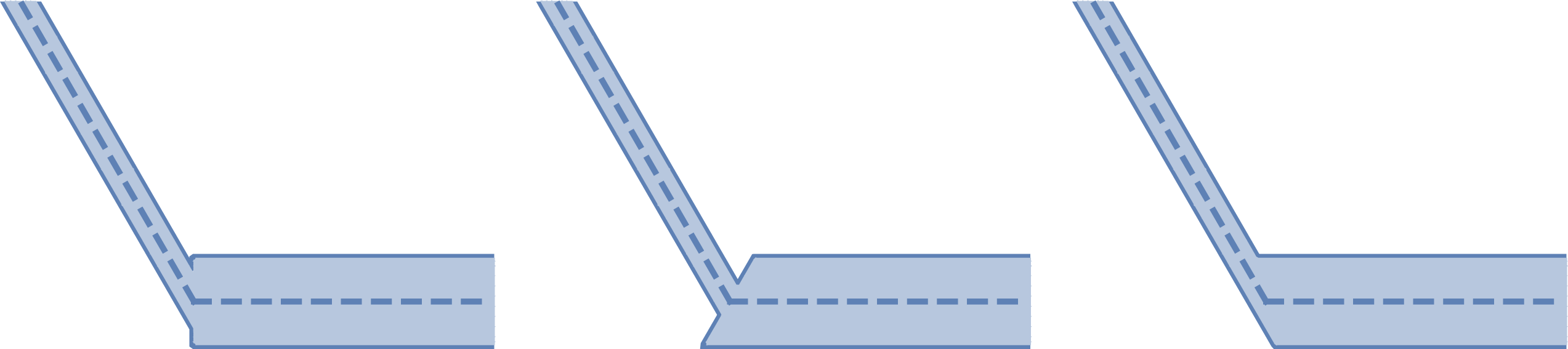
One significant deficiency in our model is the lack of a unique evolution law for a junction between viscidas of different thicknesses. In such cases, one could introduce some local smoothing and then compute the relevant integrals of the form (5.9), accepting that the local behaviour then depends on the specific choice of smoothing. Alternatively, one could obtain the required evolution law by solving an inner Stokes-flow problem, although this would still depend on defining the precise way in which the viscidas are joined. Even for the simplest case of just two viscidas, one can easily imagine a variety of ways to connect them, as illustrated in figure 16, and our analysis suggests that each would result in a different local model for the dynamics at the corner. Still, we hypothesize that any junction between
 $n$
viscidas will ultimately approach a state where the interior angles are all equal to
 $2\unicode[STIX]{x03C0}/n$
, regardless of the initial conditions. In principle, one can thus calculate at least the large-
 $\unicode[STIX]{x1D70F}$
behaviour of the entire network, which would correspond to the behaviour of a fibre cross-section far downstream of the inlet point.
The theory presented here provides an approach to the previously open problem of how to model the evolution of complex microstructured optical fibres with closely spaced holes. While our simple example solutions appear to be consistent with experimental results such as those shown in figure 3, it would be worthwhile to perform a systematic comparison between our model and experiments, as well as to study the region of overlap between the present theory and the corresponding theories for well-spaced holes (for example Buchak et al. Reference Buchak, Crowdy, Stokes and Ebendorff-Heidepriem2015).
Acknowledgements
We are grateful for the feedback from three anonymous referees, whose helpful suggestions significantly improved this paper. I.M.G. gratefully acknowledges funding from the Royal Society through a University Research Fellowship.
Appendix A. Solution strategy for a three-viscida network
Upon integration of (4.24) twice with respect to
 $\unicode[STIX]{x1D709}_{i}$
, we obtain
 $$\begin{eqnarray}\frac{\unicode[STIX]{x2202}}{\unicode[STIX]{x2202}\unicode[STIX]{x1D70F}}\left[\left(1+\frac{\unicode[STIX]{x1D70F}}{2}\right)\unicode[STIX]{x1D703}_{i}\right]=A_{i}(\unicode[STIX]{x1D70F})\int _{0}^{\unicode[STIX]{x1D709}_{i}}Y_{i}(\hat{\unicode[STIX]{x1D709}},\unicode[STIX]{x1D70F})\,\text{d}\hat{\unicode[STIX]{x1D709}}+B_{i}(\unicode[STIX]{x1D70F})\int _{0}^{\unicode[STIX]{x1D709}_{i}}X_{i}(\hat{\unicode[STIX]{x1D709}},\unicode[STIX]{x1D70F})\,\text{d}\hat{\unicode[STIX]{x1D709}}+C_{i}(\unicode[STIX]{x1D70F})\unicode[STIX]{x1D709}_{i}+D_{i}(\unicode[STIX]{x1D70F}),\end{eqnarray}$$
where
 $$\begin{eqnarray}X_{i}(\unicode[STIX]{x1D709},\unicode[STIX]{x1D70F})=X_{0}(\unicode[STIX]{x1D70F})+\int _{0}^{\unicode[STIX]{x1D709}_{i}}\cos \unicode[STIX]{x1D703}_{i}(\hat{\unicode[STIX]{x1D709}},\unicode[STIX]{x1D70F})\,\text{d}\hat{\unicode[STIX]{x1D709}},\quad Y_{i}(\unicode[STIX]{x1D709},\unicode[STIX]{x1D70F})=Y_{0}(\unicode[STIX]{x1D70F})+\int _{0}^{\unicode[STIX]{x1D709}_{i}}\sin \unicode[STIX]{x1D703}_{i}(\hat{\unicode[STIX]{x1D709}},\unicode[STIX]{x1D70F})\,\text{d}\hat{\unicode[STIX]{x1D709}}.\end{eqnarray}$$
We will fix the arbitrary rigid-body translation
 $(X_{0}(\unicode[STIX]{x1D70F}),Y_{0}(\unicode[STIX]{x1D70F}))$
later through a convenient choice to simplify the algebra. By applying the moment condition (4.26), the four angle conditions (4.27) and the force balances (4.28), we obtain the relations
 $$\begin{eqnarray}\displaystyle & \displaystyle C_{1}+C_{2}+C_{3}=0, & \displaystyle\end{eqnarray}$$
 $$\begin{eqnarray}\displaystyle & \displaystyle D_{1}-D_{3}=D_{3}-D_{2}=\frac{\unicode[STIX]{x03C0}}{3}, & \displaystyle\end{eqnarray}$$
 $$\begin{eqnarray}\displaystyle & \displaystyle \ell _{3}[A_{3}\overline{Y_{3}}+B_{3}\overline{X_{3}}+C_{3}]-\ell _{1}[A_{1}\overline{Y_{1}}+B_{1}\overline{X_{1}}+C_{1}]=\frac{2\unicode[STIX]{x03C0}}{3}, & \displaystyle\end{eqnarray}$$
 $$\begin{eqnarray}\displaystyle & \displaystyle \ell _{2}[A_{2}\overline{Y_{2}}+B_{2}\overline{X_{2}}+C_{2}]-\ell _{3}[A_{3}\overline{Y_{3}}+B_{3}\overline{X_{3}}+C_{3}]=\frac{2\unicode[STIX]{x03C0}}{3}, & \displaystyle\end{eqnarray}$$
 $$\begin{eqnarray}\overline{\unicode[STIX]{x1D719}}(\unicode[STIX]{x1D70F})=\frac{1}{\ell _{i}}\int _{0}^{\ell _{i}}\unicode[STIX]{x1D719}(\unicode[STIX]{x1D709},\unicode[STIX]{x1D70F})\,\text{d}\unicode[STIX]{x1D709}.\end{eqnarray}$$
Without loss of generality, we fix the arbitrary rotation by taking
 $$\begin{eqnarray}D_{1}(\unicode[STIX]{x1D70F})=\frac{\unicode[STIX]{x03C0}}{3},\quad D_{2}(\unicode[STIX]{x1D70F})=-\frac{\unicode[STIX]{x03C0}}{3},\quad D_{3}(\unicode[STIX]{x1D70F})=0.\end{eqnarray}$$
It is convenient to assume that the translation
 $(X_{0}(\unicode[STIX]{x1D70F}),Y_{0}(\unicode[STIX]{x1D70F}))$
is chosen such that
 $$\begin{eqnarray}A_{1}\overline{Y_{1}}+A_{2}\overline{Y_{2}}+A_{3}\overline{Y_{3}}=B_{1}\overline{X_{1}}+B_{2}\overline{X_{2}}+B_{3}\overline{X_{3}}=0.\end{eqnarray}$$
Then, equation (A 3) allows us to solve for the unknowns
 $C_{i}(\unicode[STIX]{x1D70F})$
in the forms
 $$\begin{eqnarray}\displaystyle C_{1} & = & \displaystyle -\frac{2\unicode[STIX]{x03C0}(\ell _{2}+2\ell _{3})}{3(\ell _{1}\ell _{2}+\ell _{2}\ell _{3}+\ell _{3}\ell _{1})}-(A_{1}\overline{Y_{1}}+B_{1}\overline{X_{1}}),\end{eqnarray}$$
 $$\begin{eqnarray}\displaystyle C_{2} & = & \displaystyle \frac{2\unicode[STIX]{x03C0}(\ell _{1}+2\ell _{3})}{3(\ell _{1}\ell _{2}+\ell _{2}\ell _{3}+\ell _{3}\ell _{1})}-(A_{2}\overline{Y_{2}}+B_{2}\overline{X_{2}}),\end{eqnarray}$$
 $C_{3}=-C_{1}-C_{2}$
.
Finally, to determine
 $A_{i}$
and
 $B_{i}$
, we multiply (A 1) by
 $\cos \unicode[STIX]{x1D703}_{i}$
and
 $\sin \unicode[STIX]{x1D703}_{i}$
, integrate from
 $\unicode[STIX]{x1D709}_{i}=0$
to
 $\unicode[STIX]{x1D709}_{i}=\ell _{i}$
and then subtract relevant pairs of the resulting integrated equations. Using the force balances (4.28) to eliminate
 $A_{3}$
and
 $B_{3}$
, we thus obtain a linear system whose solution at every time
 $\unicode[STIX]{x1D70F}$
yields
 $A_{1}$
,
 $A_{2}$
,
 $B_{1}$
and
 $B_{2}$
, as follows:
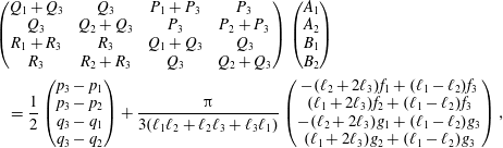 $$\begin{eqnarray}\displaystyle & & \displaystyle \left(\begin{array}{@{}cccc@{}}Q_{1}+Q_{3} & Q_{3} & P_{1}+P_{3} & P_{3}\\ Q_{3} & Q_{2}+Q_{3} & P_{3} & P_{2}+P_{3}\\ R_{1}+R_{3} & R_{3} & Q_{1}+Q_{3} & Q_{3}\\ R_{3} & R_{2}+R_{3} & Q_{3} & Q_{2}+Q_{3}\end{array}\right)\left(\begin{array}{@{}c@{}}A_{1}\\ A_{2}\\ B_{1}\\ B_{2}\end{array}\right)\nonumber\\ \displaystyle & & \displaystyle \quad =\frac{1}{2}\left(\begin{array}{@{}c@{}}p_{3}-p_{1}\\ p_{3}-p_{2}\\ q_{3}-q_{1}\\ q_{3}-q_{2}\end{array}\right)+\frac{\unicode[STIX]{x03C0}}{3(\ell _{1}\ell _{2}+\ell _{2}\ell _{3}+\ell _{3}\ell _{1})}\left(\begin{array}{@{}c@{}}-(\ell _{2}+2\ell _{3})f_{1}+(\ell _{1}-\ell _{2})f_{3}\\ (\ell _{1}+2\ell _{3})f_{2}+(\ell _{1}-\ell _{2})f_{3}\\ -(\ell _{2}+2\ell _{3})g_{1}+(\ell _{1}-\ell _{2})g_{3}\\ (\ell _{1}+2\ell _{3})g_{2}+(\ell _{1}-\ell _{2})g_{3}\end{array}\right),\qquad\end{eqnarray}$$
where we have introduced the shorthand
 $$\begin{eqnarray}P_{i}=\ell _{i}(\overline{X_{i}^{2}}-\overline{X_{i}}^{2}),\quad Q_{i}=\ell _{i}(\overline{X_{i}Y_{i}}-\overline{X_{i}}\,\overline{Y_{i}}),\quad R_{i}=\ell _{i}(\overline{Y_{i}^{2}}-\overline{Y_{i}}^{2}),\end{eqnarray}$$
 $$\begin{eqnarray}p_{i}=\ell _{i}\overline{\unicode[STIX]{x1D703}_{i}\cos \unicode[STIX]{x1D703}_{i}},\quad q_{i}=\ell _{i}\overline{\unicode[STIX]{x1D703}_{i}\sin \unicode[STIX]{x1D703}_{i}},\end{eqnarray}$$
 $$\begin{eqnarray}f_{i}=\ell _{i}\overline{(2\unicode[STIX]{x1D709}-\ell _{i})\cos \unicode[STIX]{x1D703}_{i}},\quad g_{i}=\ell _{i}\overline{(2\unicode[STIX]{x1D709}-\ell _{i})\sin \unicode[STIX]{x1D703}_{i}}.\end{eqnarray}$$
We now solve by using the method of lines, i.e. by discretizing in
 $\unicode[STIX]{x1D709}_{i}$
to turn the evolution equations (A 1) into a system of ordinary differential equations in
 $\unicode[STIX]{x1D70F}$
, with
 $A_{i}$
and
 $B_{i}$
determined at each instant by (A 8). The resulting system is then integrated using a numerical initial-value problem solver.
Appendix B. Solution strategy for a general viscida network
Integration of (4.30) with respect to
 $\unicode[STIX]{x1D709}$
and application of the boundary condition (4.33) leads to
 $$\begin{eqnarray}\frac{\unicode[STIX]{x2202}}{\unicode[STIX]{x2202}\unicode[STIX]{x1D70F}}\left[\left(1+\frac{\unicode[STIX]{x1D70F}}{2}\right)\frac{\unicode[STIX]{x2202}\unicode[STIX]{x1D703}_{ij}}{\unicode[STIX]{x2202}\unicode[STIX]{x1D709}}\right]=M_{ij}(\unicode[STIX]{x1D70F})+A_{ij}(\unicode[STIX]{x1D70F})[Y_{ij}(\unicode[STIX]{x1D709},\unicode[STIX]{x1D70F})-Y_{i}(\unicode[STIX]{x1D70F})]+B_{ij}(\unicode[STIX]{x1D70F})[X_{ij}(\unicode[STIX]{x1D709},\unicode[STIX]{x1D70F})-X_{i}(\unicode[STIX]{x1D70F})],\end{eqnarray}$$
where
 $$\begin{eqnarray}\left(\begin{array}{@{}c@{}}X_{ij}(\unicode[STIX]{x1D709},\unicode[STIX]{x1D70F})\\ Y_{ij}(\unicode[STIX]{x1D709},\unicode[STIX]{x1D70F})\end{array}\right)=\left(\begin{array}{@{}c@{}}X_{i}(\unicode[STIX]{x1D70F})\\ Y_{i}(\unicode[STIX]{x1D70F})\end{array}\right)+\int _{0}^{\unicode[STIX]{x1D709}}\left(\begin{array}{@{}c@{}}\cos \unicode[STIX]{x1D703}_{ij}(\hat{\unicode[STIX]{x1D709}},\unicode[STIX]{x1D70F})\\ \sin \unicode[STIX]{x1D703}_{ij}(\hat{\unicode[STIX]{x1D709}},\unicode[STIX]{x1D70F})\end{array}\right)\text{d}\hat{\unicode[STIX]{x1D709}},\end{eqnarray}$$
where
 $\unicode[STIX]{x1D709}\in (0,\ell _{ij})$
is the Lagrangian parametrization of viscida
 $(ij)$
at time
 $\unicode[STIX]{x1D70F}$
. By integrating once more and using the angle condition (4.37) at
 $\unicode[STIX]{x1D709}=0$
, we obtain
 $$\begin{eqnarray}\displaystyle & & \displaystyle \frac{\unicode[STIX]{x2202}}{\unicode[STIX]{x2202}\unicode[STIX]{x1D70F}}\left[\left(1+\frac{\unicode[STIX]{x1D70F}}{2}\right)[\unicode[STIX]{x1D703}_{ij}(\unicode[STIX]{x1D709},\unicode[STIX]{x1D70F})-\unicode[STIX]{x1D6E9}_{i}(\unicode[STIX]{x1D70F})]\right]-\frac{\left(v_{i}^{-1}(j)-1\right)\unicode[STIX]{x03C0}}{n_{i}}\nonumber\\ \displaystyle & & \displaystyle \quad =M_{ij}(\unicode[STIX]{x1D70F})\unicode[STIX]{x1D709}+A_{ij}(\unicode[STIX]{x1D70F})\int _{0}^{\unicode[STIX]{x1D709}}(\unicode[STIX]{x1D709}-\hat{\unicode[STIX]{x1D709}})\sin \unicode[STIX]{x1D703}_{ij}(\hat{\unicode[STIX]{x1D709}},\unicode[STIX]{x1D70F})\,\text{d}\hat{\unicode[STIX]{x1D709}}+B_{ij}(\unicode[STIX]{x1D70F})\int _{0}^{\unicode[STIX]{x1D709}}(\unicode[STIX]{x1D709}-\hat{\unicode[STIX]{x1D709}})\cos \unicode[STIX]{x1D703}_{ij}(\hat{\unicode[STIX]{x1D709}},\unicode[STIX]{x1D70F})\,\text{d}\hat{\unicode[STIX]{x1D709}}.\nonumber\\ \displaystyle & & \displaystyle\end{eqnarray}$$
Now applying the angle condition (4.37) at the other end
 $\unicode[STIX]{x1D709}=\ell _{ij}$
, we find the following relation
 $$\begin{eqnarray}\displaystyle & & \displaystyle \frac{\text{d}}{\text{d}\unicode[STIX]{x1D70F}}\left[\left(1+\frac{\unicode[STIX]{x1D70F}}{2}\right)[\unicode[STIX]{x1D6E9}_{j}(\unicode[STIX]{x1D70F})\pm \unicode[STIX]{x03C0}-\unicode[STIX]{x1D6E9}_{i}(\unicode[STIX]{x1D70F})]\right]+\frac{(v_{j}^{-1}(i)-1)\unicode[STIX]{x03C0}}{n_{j}}-\frac{(v_{i}^{-1}(j)-1)\unicode[STIX]{x03C0}}{n_{i}}\nonumber\\ \displaystyle & & \displaystyle \quad =\ell _{ij}[M_{ij}(\unicode[STIX]{x1D70F})+A_{ij}(\unicode[STIX]{x1D70F})\overline{(Y_{ij}-Y_{i})}(\unicode[STIX]{x1D70F})+B_{ij}(\unicode[STIX]{x1D70F})\overline{(X_{ij}-X_{i})}(\unicode[STIX]{x1D70F})]\end{eqnarray}$$
 $$\begin{eqnarray}\displaystyle & & \displaystyle \quad =-\ell _{ji}[M_{ji}(\unicode[STIX]{x1D70F})+A_{ji}(\unicode[STIX]{x1D70F})\overline{(Y_{ji}-Y_{j})}(\unicode[STIX]{x1D70F})+B_{ji}(\unicode[STIX]{x1D70F})\overline{(X_{ji}-X_{j})}(\unicode[STIX]{x1D70F})],\end{eqnarray}$$
 $(i,j)$
, defined as in (A 4), and the latter identity in (B 4) follows from the symmetry condition (4.34).
Equation (B 4) relates the relative rate of rotation of junctions
 $i$
and
 $j$
to the tensions and moments in the viscida that connects them. It is worth noting that the second and third terms on the left-hand side of (B 4), and the sign of the
 $\pm \unicode[STIX]{x03C0}$
inside the first term, are all fixed in advance once the initial topology of the network has been established.
Next we multiply (B 3) by
 $(\sin \unicode[STIX]{x1D703}_{ij},\cos \unicode[STIX]{x1D703}_{ij})$
and integrate between
 $\unicode[STIX]{x1D709}=0$
and
 $\unicode[STIX]{x1D709}=\ell _{ij}$
to get
 $$\begin{eqnarray}\displaystyle & & \displaystyle \left(1+\frac{\unicode[STIX]{x1D70F}}{2}\right)\frac{\text{d}}{\text{d}\unicode[STIX]{x1D70F}}[X_{j}(\unicode[STIX]{x1D70F})-X_{i}(\unicode[STIX]{x1D70F})]\nonumber\\ \displaystyle & & \displaystyle \quad +\,\left[\frac{\text{d}}{\text{d}\unicode[STIX]{x1D70F}}\left[\left(1+\frac{\unicode[STIX]{x1D70F}}{2}\right)\unicode[STIX]{x1D6E9}_{i}(\unicode[STIX]{x1D70F})\right]+\frac{\left(v_{i}^{-1}(j)-1\right)\unicode[STIX]{x03C0}}{n_{i}}\right][Y_{j}(\unicode[STIX]{x1D70F})-Y_{i}(\unicode[STIX]{x1D70F})]\nonumber\\ \displaystyle & & \displaystyle \quad -\,\frac{1}{2}\ell _{ij}\overline{\unicode[STIX]{x1D703}_{ij}\sin \unicode[STIX]{x1D703}_{ij}}(\unicode[STIX]{x1D70F})=\ell _{ij}M_{ij}(\unicode[STIX]{x1D70F})\overline{(Y_{ij}-Y_{j})}(\unicode[STIX]{x1D70F})\nonumber\\ \displaystyle & & \displaystyle \quad +\,\ell _{ij}A_{ij}(\unicode[STIX]{x1D70F})\overline{(Y_{ij}-Y_{i})(Y_{ij}-Y_{j})}(\unicode[STIX]{x1D70F})+\ell _{ij}B_{ij}(\unicode[STIX]{x1D70F})\overline{(X_{ij}-X_{i})(Y_{ij}-Y_{j})}(\unicode[STIX]{x1D70F}),\end{eqnarray}$$
and
 $$\begin{eqnarray}\displaystyle & & \displaystyle \left(1+\frac{\unicode[STIX]{x1D70F}}{2}\right)\frac{\text{d}}{\text{d}\unicode[STIX]{x1D70F}}[Y_{j}(\unicode[STIX]{x1D70F})-Y_{i}(\unicode[STIX]{x1D70F})]\nonumber\\ \displaystyle & & \displaystyle \quad -\,\left[\frac{\text{d}}{\text{d}\unicode[STIX]{x1D70F}}\left[\left(1+\frac{\unicode[STIX]{x1D70F}}{2}\right)\unicode[STIX]{x1D6E9}_{i}(\unicode[STIX]{x1D70F})\right]+\frac{(v_{i}^{-1}(j)-1)\unicode[STIX]{x03C0}}{n_{i}}\right][X_{j}(\unicode[STIX]{x1D70F})-X_{i}(\unicode[STIX]{x1D70F})]\nonumber\\ \displaystyle & & \displaystyle \quad +\,\frac{1}{2}\ell _{ij}\overline{\unicode[STIX]{x1D703}_{ij}\cos \unicode[STIX]{x1D703}_{ij}}(\unicode[STIX]{x1D70F})=-\ell _{ij}M_{ij}(\unicode[STIX]{x1D70F})\overline{(X_{ij}-X_{j})}(\unicode[STIX]{x1D70F})\nonumber\\ \displaystyle & & \displaystyle \quad -\,\ell _{ij}A_{ij}(\unicode[STIX]{x1D70F})\overline{(X_{ij}-X_{j})(Y_{ij}-Y_{i})}(\unicode[STIX]{x1D70F})-\ell _{ij}B_{ij}(\unicode[STIX]{x1D70F})\overline{(X_{ij}-X_{i})(X_{ij}-X_{j})}(\unicode[STIX]{x1D70F}).\end{eqnarray}$$
It can be verified that the corresponding versions of (B 5) and (B 6) with the indices
 $(i,j)$
swapped are satisfied identically by virtue of (B 4) and the symmetry relations (4.31) and (4.34).
Let us suppose, as suggested in § 4.3, that we have eliminated the arbitrary rigid-body motion by fixing the position and rotation angle at vertex 1. For each of the
 $N$
viscidas, indexed by
 $(i,j)$
, equations (B 4), (B 5) and (B 6) provide a
 $3\times 3$
linear system that instantaneously determines the tensions
 $A_{ij}$
,
 $B_{ij}$
and moment
 $M_{ij}$
. If we solve all of the
 $N$
such linear systems and substitute the results into the force and moment balances (4.39), then we end up with
 $3J-3$
independent linear equations for the velocities
 $\text{d}/\text{d}\unicode[STIX]{x1D70F}(X_{i}(\unicode[STIX]{x1D70F}),Y_{i}(\unicode[STIX]{x1D70F}))$
and rotation rates
 $\text{d}/\text{d}\unicode[STIX]{x1D70F}((1+\unicode[STIX]{x1D70F}/2)\unicode[STIX]{x1D6E9}_{i}(\unicode[STIX]{x1D70F}))$
of all of the
 $J-1$
remaining junctions, with
 $i=2,3,\ldots ,J$
.
Thus the velocity and rotation rate of every junction is instantaneously determined, in terms of the shape of each viscida (through the averaged quantities
 $\overline{X_{ij}}$
,
 $\overline{\unicode[STIX]{x1D703}_{ij}\sin \unicode[STIX]{x1D703}_{ij}}$
, etc.) and the position of each junction. If we now discretize each
 $\unicode[STIX]{x1D703}_{ij}(\unicode[STIX]{x1D709},\unicode[STIX]{x1D70F})$
in
 $\unicode[STIX]{x1D709}$
, using say
 $m$
grid points, then the whole problem is reduced to a system of
 $3J-3+Nm$
ordinary differential equations in
 $\unicode[STIX]{x1D70F}$
, which can be tackled using a standard solver.
Appendix C. The evolution of a clamped viscida
By integrating (2.9) twice with respect to
 $\unicode[STIX]{x1D709}$
and applying the clamped boundary condition (5.7a
) at
 $\unicode[STIX]{x1D709}=0$
, we obtain
 $$\begin{eqnarray}\displaystyle \frac{\unicode[STIX]{x2202}\unicode[STIX]{x1D703}}{\unicode[STIX]{x2202}\unicode[STIX]{x1D70F}} & = & \displaystyle -\frac{1}{2}\left(\frac{\unicode[STIX]{x1D703}(\unicode[STIX]{x1D709},\unicode[STIX]{x1D70F})}{h_{0}(\unicode[STIX]{x1D709})+\unicode[STIX]{x1D70F}/2}-\frac{\unicode[STIX]{x1D703}(0,0)}{h_{0}(0)+\unicode[STIX]{x1D70F}/2}\right)-\frac{1}{2}\int _{0}^{\unicode[STIX]{x1D709}}\frac{h_{0}^{\prime }(\hat{\unicode[STIX]{x1D709}})\unicode[STIX]{x1D703}(\hat{\unicode[STIX]{x1D709}},\unicode[STIX]{x1D70F})}{(h_{0}(\hat{\unicode[STIX]{x1D709}})+\unicode[STIX]{x1D70F}/2)^{2}}\,\text{d}\hat{\unicode[STIX]{x1D709}}\nonumber\\ \displaystyle & & \displaystyle +\,3A(\unicode[STIX]{x1D70F})\int _{0}^{\unicode[STIX]{x1D709}}\frac{h_{0}(\hat{\unicode[STIX]{x1D709}})y(\hat{\unicode[STIX]{x1D709}},\unicode[STIX]{x1D70F})}{(h_{0}(\hat{\unicode[STIX]{x1D709}})+\unicode[STIX]{x1D70F}/2)^{4}}\,\text{d}\hat{\unicode[STIX]{x1D709}}-3B(\unicode[STIX]{x1D70F})\int _{0}^{\unicode[STIX]{x1D709}}\frac{h_{0}(\hat{\unicode[STIX]{x1D709}})x(\hat{\unicode[STIX]{x1D709}},\unicode[STIX]{x1D70F})}{(h_{0}(\hat{\unicode[STIX]{x1D709}})+\unicode[STIX]{x1D70F}/2)^{4}}\,\text{d}\hat{\unicode[STIX]{x1D709}}\nonumber\\ \displaystyle & & \displaystyle +\,C(\unicode[STIX]{x1D70F})\int _{0}^{\unicode[STIX]{x1D709}}\frac{h_{0}(\hat{\unicode[STIX]{x1D709}})}{(h_{0}(\hat{\unicode[STIX]{x1D709}})+\unicode[STIX]{x1D70F}/2)^{4}}\,\text{d}\hat{\unicode[STIX]{x1D709}},\end{eqnarray}$$
where
 $C(\unicode[STIX]{x1D70F})$
is a function of integration to be determined. Imposing the clamped-angle condition (5.7b
) at
 $\unicode[STIX]{x1D709}=1$
, we obtain
 $$\begin{eqnarray}\displaystyle & & \displaystyle 3\widetilde{y}(\unicode[STIX]{x1D70F})A(\unicode[STIX]{x1D70F})-3\widetilde{x}(\unicode[STIX]{x1D70F})B(\unicode[STIX]{x1D70F})+\widetilde{1}(\unicode[STIX]{x1D70F})C(\unicode[STIX]{x1D70F})\nonumber\\ \displaystyle & & \displaystyle \quad =\frac{\unicode[STIX]{x1D703}(1,0)}{2h_{0}(1)+\unicode[STIX]{x1D70F}}-\frac{\unicode[STIX]{x1D703}(0,0)}{2h_{0}(0)+\unicode[STIX]{x1D70F}}+\frac{1}{2}\int _{0}^{1}\frac{h_{0}^{\prime }(\unicode[STIX]{x1D709})\unicode[STIX]{x1D703}(\unicode[STIX]{x1D709},\unicode[STIX]{x1D70F})}{(h_{0}(\unicode[STIX]{x1D709})+\unicode[STIX]{x1D70F}/2)^{2}}\,\text{d}\unicode[STIX]{x1D709},\end{eqnarray}$$
where, for any
 $\unicode[STIX]{x1D719}(\unicode[STIX]{x1D709},\unicode[STIX]{x1D70F})$
, we define the weighted average
 $$\begin{eqnarray}\widetilde{\unicode[STIX]{x1D719}}(\unicode[STIX]{x1D70F})=\int _{0}^{1}\frac{h_{0}(\unicode[STIX]{x1D709})}{(h_{0}(\unicode[STIX]{x1D709})+\unicode[STIX]{x1D70F}/2)^{4}}\unicode[STIX]{x1D719}(\unicode[STIX]{x1D709},\unicode[STIX]{x1D70F})\,\text{d}\unicode[STIX]{x1D709}.\end{eqnarray}$$
Similarly, by multiplying (C 1) by
 $(\cos \unicode[STIX]{x1D703},\sin \unicode[STIX]{x1D703})$
, integrating over the viscida length, from
 $\unicode[STIX]{x1D709}=0$
to
 $\unicode[STIX]{x1D709}=1$
, and applying the boundary conditions (5.7), we obtain
 $$\begin{eqnarray}\displaystyle & & \displaystyle 3\widetilde{y^{2}}(\unicode[STIX]{x1D70F})A(\unicode[STIX]{x1D70F})-3\widetilde{xy}(\unicode[STIX]{x1D70F})B(\unicode[STIX]{x1D70F})+\widetilde{y}(\unicode[STIX]{x1D70F})C(\unicode[STIX]{x1D70F})\nonumber\\ \displaystyle & & \displaystyle \quad =\frac{1}{2}\int _{0}^{1}\frac{h_{0}(\unicode[STIX]{x1D709})\cos \unicode[STIX]{x1D703}(\unicode[STIX]{x1D709},\unicode[STIX]{x1D70F})-h_{0}(\unicode[STIX]{x1D709})\unicode[STIX]{x1D703}(\unicode[STIX]{x1D709},\unicode[STIX]{x1D70F})\sin \unicode[STIX]{x1D703}(\unicode[STIX]{x1D709},\unicode[STIX]{x1D70F})+h_{0}^{\prime }(\unicode[STIX]{x1D709})y(\unicode[STIX]{x1D709},\unicode[STIX]{x1D70F})\unicode[STIX]{x1D703}(\unicode[STIX]{x1D709},\unicode[STIX]{x1D70F})}{(h_{0}(\unicode[STIX]{x1D709})+\unicode[STIX]{x1D70F}/2)^{2}}\,\text{d}\unicode[STIX]{x1D709},\nonumber\\ \displaystyle & & \displaystyle\end{eqnarray}$$
and
 $$\begin{eqnarray}\displaystyle & & \displaystyle 3[\widetilde{xy}(\unicode[STIX]{x1D70F})-x(1,0)\widetilde{y}(\unicode[STIX]{x1D70F})]A(\unicode[STIX]{x1D70F})-3[\widetilde{x^{2}}(\unicode[STIX]{x1D70F})-x(1,0)\widetilde{x}(\unicode[STIX]{x1D70F})]B(\unicode[STIX]{x1D70F})+[\vphantom{\widetilde{x^{2}}}\widetilde{x}(\unicode[STIX]{x1D70F})-x(1,0)\widetilde{1}(\unicode[STIX]{x1D70F})]C(\unicode[STIX]{x1D70F})\nonumber\\ \displaystyle & & \displaystyle \quad =\frac{\unicode[STIX]{x1D703}(0,0)x(1,0)}{2h_{0}(0)+\unicode[STIX]{x1D70F}}+\frac{1}{2}\int _{0}^{1}\nonumber\\ \displaystyle & & \displaystyle \quad \times \,\frac{h_{0}(\unicode[STIX]{x1D709})\sin \unicode[STIX]{x1D703}(\unicode[STIX]{x1D709},\unicode[STIX]{x1D70F})-h_{0}(\unicode[STIX]{x1D709})\unicode[STIX]{x1D703}(\unicode[STIX]{x1D709},\unicode[STIX]{x1D70F})\cos \unicode[STIX]{x1D703}(\unicode[STIX]{x1D709},\unicode[STIX]{x1D70F})+h_{0}^{\prime }(\unicode[STIX]{x1D709})[x(\unicode[STIX]{x1D709},\unicode[STIX]{x1D70F})-x(1,0)]\unicode[STIX]{x1D703}(\unicode[STIX]{x1D709},\unicode[STIX]{x1D70F})}{(h_{0}(\unicode[STIX]{x1D709})+\unicode[STIX]{x1D70F}/2)^{2}}\,\text{d}\unicode[STIX]{x1D709}.\nonumber\\ \displaystyle & & \displaystyle\end{eqnarray}$$
The solution of the linear system (C 2), (C 4), (C 5) determines the three unknown functions
 $A(\unicode[STIX]{x1D70F})$
,
 $B(\unicode[STIX]{x1D70F})$
and
 $C(\unicode[STIX]{x1D70F})$
at each time
 $\unicode[STIX]{x1D70F}$
. The evolution equation (C 1) is then solved by discretizing in
 $\unicode[STIX]{x1D709}$
and using the method of lines.