1 Introduction
Inkjet technology is a vital technology that is widely used in applications, including 3D printing (Vaezi, Seitz & Yang Reference Vaezi, Seitz and Yang2013), bioengineering (Murphy & Atala Reference Murphy and Atala2014) and manufacturing microelectronic devices (Calvert Reference Calvert2001; Gao et al. Reference Gao, Ng, Furlani, Chwalek and Hawkins2010). The technology was first developed in the nineteenth century by Lord Rayleigh (Reference Rayleigh1878). Afterwards, the field received much attention aimed toward investigating fundamental mechanisms and technologies that can enable one to realize high quality products at low cost. The main feature of the technology involves transporting a particular fluid with/without particles onto a substrate in an accurate way. To realize precise deposition of droplets, a detailed study of the fluid mechanics of droplet formation is necessary.
Studies focused on evaluating droplet formation and seeking optimum conditions for steady ejection have been conducted using both experimental and numerical methods. Bogy & Talke (Reference Bogy and Talke1984) gained insight into the drop-on-demand (DOD) inkjet phenomena, which are related to acoustic waves within the inkjet cavity, with a good experimental verification. Zhang & Basaran (Reference Zhang and Basaran1995) classified different droplet formation dynamics by evaluating the effects of the driving forces. A stable criterion
 $Z$
defined as the ratio of the Reynolds number to Weber number was first proposed by Fromm (Reference Fromm1984), which was later widely accepted as a criterion for stability. Reis & Derby (Reference Reis and Derby2000) used computational and experimental studies to identify the optimum printing parameters, and proposed a redesigned range of
 $1<Z<10$
for stable droplet ejection. Ambravaneswaran, Wilkes & Basaran (Reference Ambravaneswaran, Wilkes and Basaran2002) compared one- and two-dimensional algorithms based on the finite element method (FEM) using Weber and Ohnesorge numbers. Duineveld & Haskal (Reference Duineveld and Haskal2002) suggested that there is a minimum velocity for drop ejection. Chen & Basaran (Reference Chen and Basaran2002) reported a method to reduce the drop radius without reducing the nozzle radius by controlling the time scales. Later, a conservative level set method was improved (Olsson & Kreiss Reference Olsson and Kreiss2005; Olsson, Kreiss & Zahedi Reference Olsson, Kreiss and Zahedi2007). Dong, Carr & Morris (Reference Dong, Carr and Morris2006a
,Reference Dong, Carr and Morris
b
) examined the effects of a signal waveform on the droplet size and satellite formation using a DOD apparatus. de Jong et al. (Reference de Jong, Versluis, de Bruin, Lohse, Reinten, van den Berg and de Jong2005, Reference de Jong, de Bruin, Reinten, van den Berg, Wijshoff, Versluis and Lohse2006) and Jong et al. (Reference Jong, Jeurissen, Borel, Berg, Wijshoff, Reinten and Lohse2006) studied the impact of an entrapped air bubble on the motion characteristics of droplets. Choi et al. (Reference Choi, Kim, Lee, Lee and Kim2015) expanded the stable printable range by adopting structural improvements. Wijshoff (Reference Wijshoff2004, Reference Wijshoff2006, Reference Wijshoff2012) delved into the acoustic mechanism inside the inkjet nozzle and gained a deep understanding of droplet formation.
Although scholars have developed effective ways to control droplet formation and have found the prior conditions necessary for a steady process, there are no reliable criteria for a multi-factor analysis including the inkjet operating conditions. The existing dimensionless numbers are inadequate for evaluation of a stable or unstable inkjet process since droplet behaviour is affected by highly coupled factors. In this paper, using a combination of experimental study and case by case modelling, the primary factors affecting droplet behaviour for the inkjet process have been obtained. A proper non-dimensional criterion concerning both the driving parameters and the nozzle dimensions for a stable inkjet process is proposed. Based on the new criterion, the optimized operating conditions can be reliably addressed as a direction in real runs.
2 Problem description
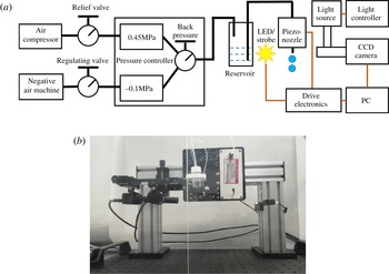
(a) Schematic diagram of the experimental apparatus, and (b) experimental devices.

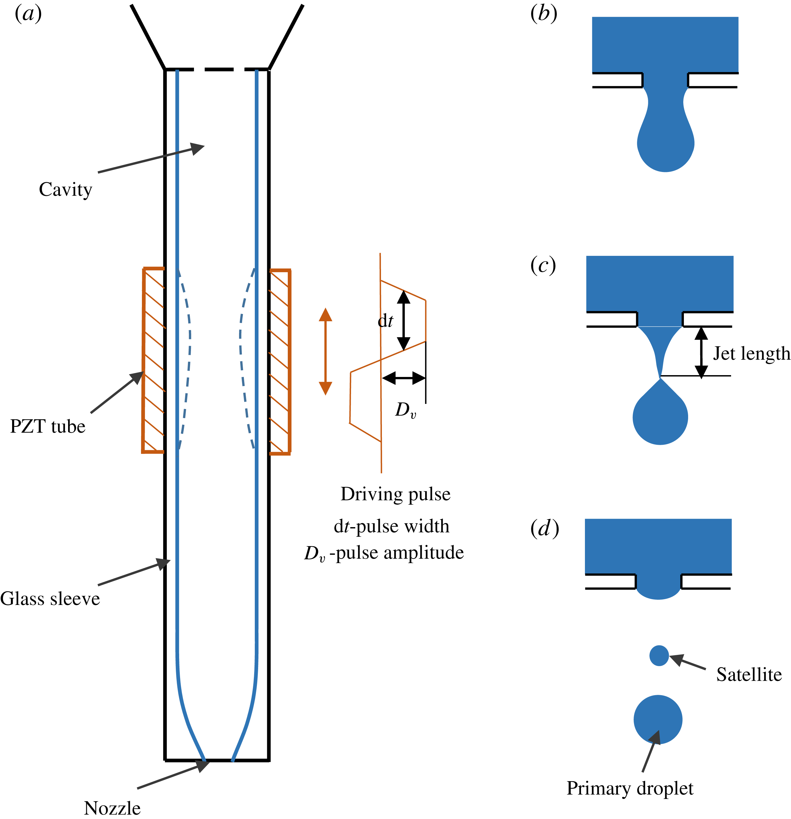
(a) Structure of the piezo-nozzle, (b) the early ejection stage, (c) the jet length at the breakup instant and (d) the droplet motion after leaving the nozzle.

A DOD piezoelectric inkjet apparatus was developed for visualizing droplet formation, as shown in figure 1. The main components of the inkjet system are a droplet generation module and a visual observation module. The former mainly contains a reservoir, piezo-nozzle, drive electronics and a precise pressure controller. A MJ-AT-01 piezo-nozzle manufactured by the MicroFab Company was used with an orifice diameter of
 $80~\unicode[STIX]{x03BC}\text{m}$
. The exposure time of the LED/strobe is approximately
 $5~\unicode[STIX]{x03BC}\text{s}$
and no longer than
 $10~\unicode[STIX]{x03BC}\text{s}$
to prevent ‘smearing’ of the drop along the trajectory. Three states are precisely switched using a pressure controller to maintain normal operation. To seal up the system, a silicone gasket is placed around the neck of the reservoir. The visual observation module consists of a CCD camera, enlarging lens and a group of micro three-dimensional displacement benches.
The DOD printers can generate a desired number of drops via a relatively easy control. In the current system, the droplets are generated by exerting a pressure pulse, which exceeds a certain threshold value at the nozzle, to release a droplet. The pressure pulse is produced by a mechanically actuated transducer based on a PZT (lead zirconium titanate) tube, with mechanical deformation actuated by a driving electric pulse, which includes the two most influential driving parameters – the pulse width and pulse amplitude. In experiments, a pulse amplitude of 40 to
 $-100~\text{V}$
and pulse width of
 $3{-}25~\unicode[STIX]{x03BC}\text{s}$
was used. Figure 2 shows the structure of the piezo-nozzle and the droplet formation process. When the pressure pulse is absent, both liquid surface tension and a static back pressure ensure that the meniscus is stable at the nozzle. When the positive wave generated counteracts surface energy, a liquid column is pushed out. Then, the negative pressure wave propagating toward the nozzle pulls the liquid back to form a droplet. A schematic for the droplet formation and motion is illustrated in figure 2(b–d). A sequence of images for the droplet motion at different delay times is captured by a CCD camera with a frame rate of 22 frames per second, a single pixel size of
 $3.75~\unicode[STIX]{x03BC}\text{m}$
and an effective resolution of
 $1280\times 960$
. The camera is equipped with a four-times magnifier, with a working distance of 65 mm. The actual size of the observed droplet can be computed according to the measured size. Both the CCD camera and the driving system are automatically controlled by a computer.
3 Mathematical model
An axisymmetric model is adopted in the simulation. The drop ejection process includes droplet formation at the nozzle followed by movement in the chamber. In the calculation, the zone from the inlet (the top of the channel) to the bottom nozzle is liquid, while the zone from the nozzle to the substrate is gas. For numerical studies, parameter ranges of
 $40{-}80~\unicode[STIX]{x03BC}\text{m}$
for the nozzle diameter,
 $0.6{-}8~\text{m}~\text{s}^{-1}$
for the inlet velocity,
 $4{-}25~\unicode[STIX]{x03BC}\text{s}$
for the pulse width,
 $500{-}2000~\text{kg}~\text{m}^{-3}$
for the liquid density, 5–30 cP for the liquid viscosity and
 $0.01{-}0.07~\text{N}~\text{m}^{-1}$
for the liquid surface tension are used. For the various simulations described below, the unstated parameters are fixed as
 $1.375~\text{m}~\text{s}^{-1}$
for the inlet velocity,
 $10~\unicode[STIX]{x03BC}\text{s}$
for the pulse width and
 $80~\unicode[STIX]{x03BC}\text{m}$
for the nozzle diameter.
A velocity boundary is given at the inlet,
 $$\begin{eqnarray}v(r)=4V_{in}\left(\frac{r+0.1\,\text{mm}}{0.2\;\text{mm}}\right)\left(1-\frac{r+0.1~\text{mm}}{0.2~\text{mm}}\right)~\text{m}~\text{s}^{-1},\end{eqnarray}$$
where
 $V_{in}$
is a given velocity constant, and
 $r$
is the radial position. The inlet diameter is 0.2 mm. The time-dependent velocity profile in the
 $r$
direction can also be calculated. Affected by viscous force, the velocity of the fluid near the wall is reduced. Along the radius, the velocity varies according to the parabolic profile in (3.1). Since the signal shown in figure 2 is a trapezoidal pulse, a step function is chosen to simulate the change in velocity with time,
 $$\begin{eqnarray}v(r,t)=(\text{step}(t-1\times 10^{-6}~\text{s})-\text{step}(t-(\text{d}t+3\times 10^{-6})\text{s}))\cdot v(r),\end{eqnarray}$$
where step (
 $t$
) is a step function for a smooth transition, and
 $t$
is time in the unit of seconds (s). The outlet is set to a constant pressure. Furthermore, no-slip conditions are given for all the walls except the substrate on which the wetting condition is adopted with a defined contact angle and a slip length.
The flow is calculated by the incompressible Navier–Stokes (N–S) equations, including the surface tension force. The equations are as follows,
 $$\begin{eqnarray}\displaystyle & \displaystyle \unicode[STIX]{x1D70C}\left(\frac{\unicode[STIX]{x2202}\boldsymbol{u}}{\unicode[STIX]{x2202}t}+\boldsymbol{u}\boldsymbol{\cdot }\unicode[STIX]{x1D735}\boldsymbol{u}\right)-\unicode[STIX]{x1D707}\unicode[STIX]{x0394}\boldsymbol{u}+\unicode[STIX]{x1D735}p=\boldsymbol{F}_{st}, & \displaystyle\end{eqnarray}$$
 $$\begin{eqnarray}\displaystyle & (\unicode[STIX]{x1D735}\boldsymbol{\cdot }\boldsymbol{u})=0, & \displaystyle\end{eqnarray}$$
where
 $\unicode[STIX]{x1D70C}$
is the density,
 $\unicode[STIX]{x1D707}$
is the dynamic viscosity,
 $\boldsymbol{u}$
is the velocity,
 $p$
is the pressure and
 $\boldsymbol{F}_{st}$
is the surface tension force, which is computed by
 $$\begin{eqnarray}\displaystyle & \boldsymbol{F}_{st}=\unicode[STIX]{x1D735}\boldsymbol{\cdot }\unicode[STIX]{x1D64F}, & \displaystyle\end{eqnarray}$$
 $$\begin{eqnarray}\displaystyle & \unicode[STIX]{x1D64F}=\unicode[STIX]{x1D70E}(\unicode[STIX]{x1D644}-(\boldsymbol{n}\boldsymbol{n}^{\text{T}}))\unicode[STIX]{x1D6FF}. & \displaystyle\end{eqnarray}$$
Here,
 $\unicode[STIX]{x1D644}$
is the identity matrix,
 $\boldsymbol{n}$
denotes the interface normal,
 $\unicode[STIX]{x1D70E}$
is the surface tension coefficient and
 $\unicode[STIX]{x1D6FF}$
is the Dirac delta function that is zero except at the fluid interface. The interface normal is calculated by
 $$\begin{eqnarray}\boldsymbol{n}=\frac{\unicode[STIX]{x1D735}\unicode[STIX]{x1D6F7}}{|\unicode[STIX]{x1D735}\unicode[STIX]{x1D6F7}|},\end{eqnarray}$$
and the delta function can be approximated by
 $$\begin{eqnarray}\unicode[STIX]{x1D6FF}=6|\unicode[STIX]{x1D6F7}(1-\unicode[STIX]{x1D6F7})|\,|\unicode[STIX]{x1D735}\unicode[STIX]{x1D6F7}|,\end{eqnarray}$$
where
 $\unicode[STIX]{x1D6F7}$
is the level set function. In the study, the contour of
 $\unicode[STIX]{x1D6F7}=0.5$
defines the interface. For the selection of the level set function, the reinitialization process can be found in the literature (Olsson & Kreiss Reference Olsson and Kreiss2005; Olsson et al.
Reference Olsson, Kreiss and Zahedi2007). The convection for the reinitialized level set function can be described by
 $$\begin{eqnarray}\frac{\unicode[STIX]{x2202}\unicode[STIX]{x1D719}}{\unicode[STIX]{x2202}t}+\unicode[STIX]{x1D735}\boldsymbol{\cdot }(\unicode[STIX]{x1D719}\boldsymbol{u})+\unicode[STIX]{x1D6FE}\left[\left(\unicode[STIX]{x1D735}\boldsymbol{\cdot }\left(\unicode[STIX]{x1D719}(1-\unicode[STIX]{x1D719})\frac{\unicode[STIX]{x1D735}\unicode[STIX]{x1D719}}{|\unicode[STIX]{x1D735}\unicode[STIX]{x1D719}|}\right)\right)-\unicode[STIX]{x1D700}\unicode[STIX]{x1D735}\boldsymbol{\cdot }\unicode[STIX]{x1D735}\unicode[STIX]{x1D719}\right]=0,\end{eqnarray}$$
where
 $\unicode[STIX]{x1D700}$
is a constant related to the thickness of the transition layer, and
 $\unicode[STIX]{x1D6FE}$
represents the maximum magnitude in the velocity field. In addition to defining the fluid interface, the level set function is used to smooth the density and viscosity jumps across the interface according to the following formulae,
 $$\begin{eqnarray}\displaystyle & \unicode[STIX]{x1D70C}=\unicode[STIX]{x1D70C}_{air}+(\unicode[STIX]{x1D70C}_{ink}-\unicode[STIX]{x1D70C}_{air})\unicode[STIX]{x1D719}, & \displaystyle\end{eqnarray}$$
 $$\begin{eqnarray}\displaystyle & \unicode[STIX]{x1D707}=\unicode[STIX]{x1D707}_{air}+(\unicode[STIX]{x1D707}_{ink}-\unicode[STIX]{x1D707}_{air})\unicode[STIX]{x1D719}. & \displaystyle\end{eqnarray}$$
4 Results and discussion
4.1 Experimental verification and parameter analysis
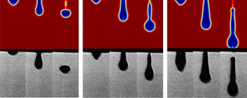
Comparison of numerical results and experimental observations for ethanol droplet behaviour with an increased driving force.
 $V_{in}$
is 0.75, 1.0,
 $1.25~\text{m}~\text{s}^{-1}$
for the simulation, and the pulse amplitude
 $D_{v}$
is 50, 70, 80 V for the experiments, respectively.

A stable droplet formation process should show fewer satellites and high reproducibility as preferred for an inkjet process with uniform and stable deposition. Reis & Derby (Reference Reis and Derby2000) once raised a notion ‘the tail behind a forming droplet is now merged with the droplet immediately behind, and thus droplets can be obtained at distances acceptable for printing’ as the definition of a stable droplet, as commonly acknowledged by others (Smith et al. Reference Smith, Shin, Stringer, Derby and Reis2006; Gardini et al. Reference Gardini, Dondi, Costa, Matteucci, Blosi, Galassi and Cinotti2008; Jungst et al. Reference Jungst, Smolan, Schacht, Scheibel and Groll2016). Therefore, in the current study, an ejection process is considered stable if no more than two satellites are formed that are subsequently merged into the primary droplet before impacting onto the substrate.
Before carrying out a formal calculation, a convergent study was carried out to obtain mesh-independent results. The grid number, larger than 3e
 $+$
04 with an averaged element quality of 0.989, is doubled and halved, respectively, until the simulation results become insensitive to the grid. Figure 3 shows a comparison between the experimental observations and simulation results. One can see that for the different stages, the predicted results agree well with the experimentally observed droplet patterns. Therefore, the applied models and assumptions are reasonable enough to obtain accurate results. When the driving force (the inlet velocity
 $V_{in}$
in the model, or the pulse amplitude
 $D_{v}$
in experiments) is weak, as shown in figure 3(a), the ejected droplet has no tail. The larger driving force leads to a long tail, which may develop into satellite droplets. For single-wave propagation in the experiments, a large driving force provides high energy, hence resulting in large droplets with high velocities.
As revealed by the experiments, the inlet velocity,
 $V_{in}$
, in (3.1) is approximately proportional to the pulse amplitude,
 $D_{v}$
. In other words, both parameters work in a similar way in driving the droplet formation. Therefore, it is reasonable to assume that the
 $D_{v}$
used in experiments is equivalent to the
 $V_{in}$
in modelling for the following studies. The droplet characteristics can be represented by the parameters at the rupture moment, including the rupture time, the jet length and the moving speed. The rupture moments for the droplets are critical for investigating droplet ejection and the moving process. After the droplet takes off from the nozzle, only the constant environment affects its behaviour. Therefore, the different rupture moments for the droplets are implicitly related to the droplet states.
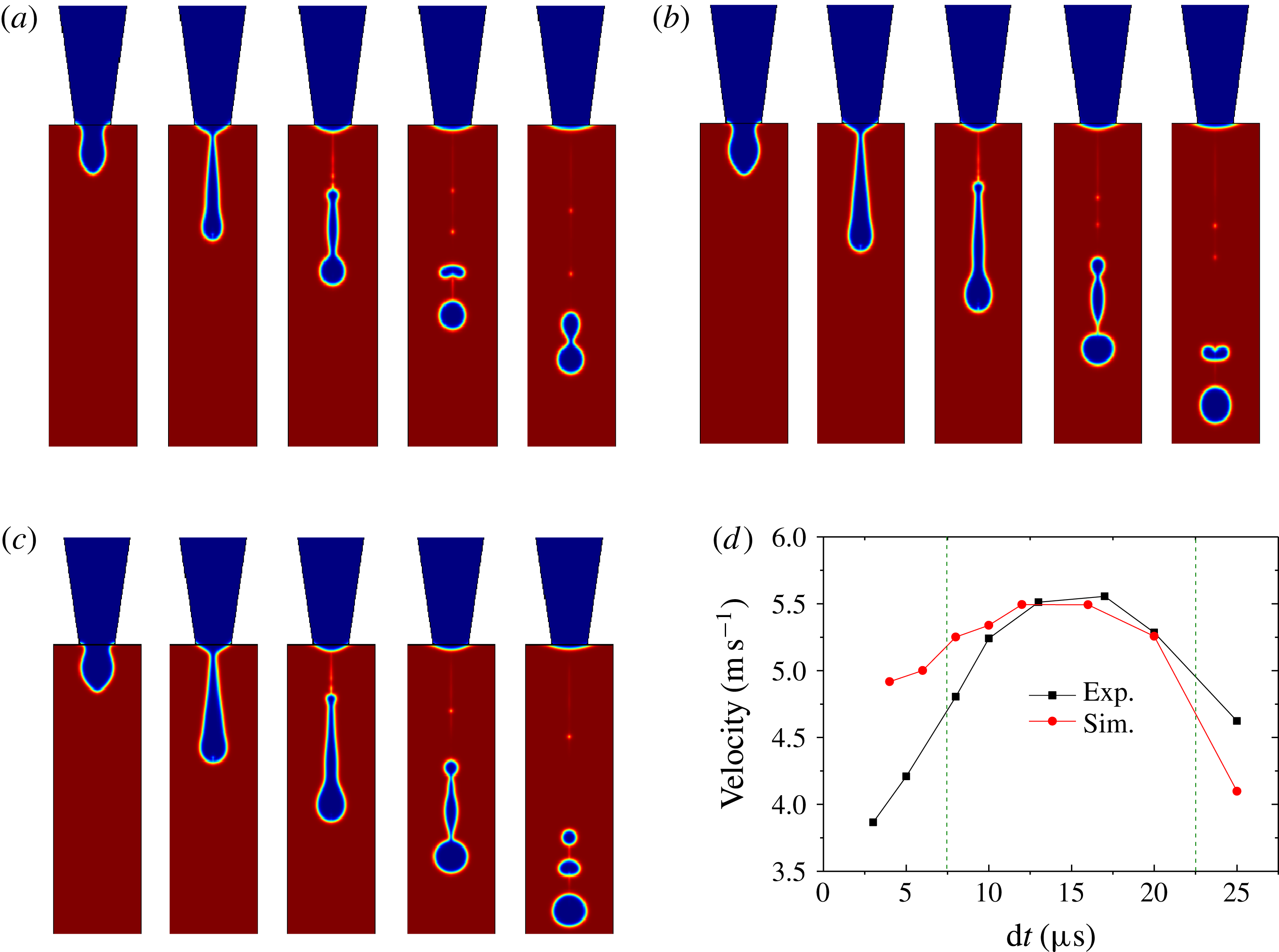
Influence of the pulse width on the jetting process for ethanol at (a)
 $6~\unicode[STIX]{x03BC}\text{s}$
, (b)
 $10~\unicode[STIX]{x03BC}\text{s}$
and (c)
 $12~\unicode[STIX]{x03BC}\text{s}$
. (d) Comparison of the predicted and experimentally measured droplet speed.
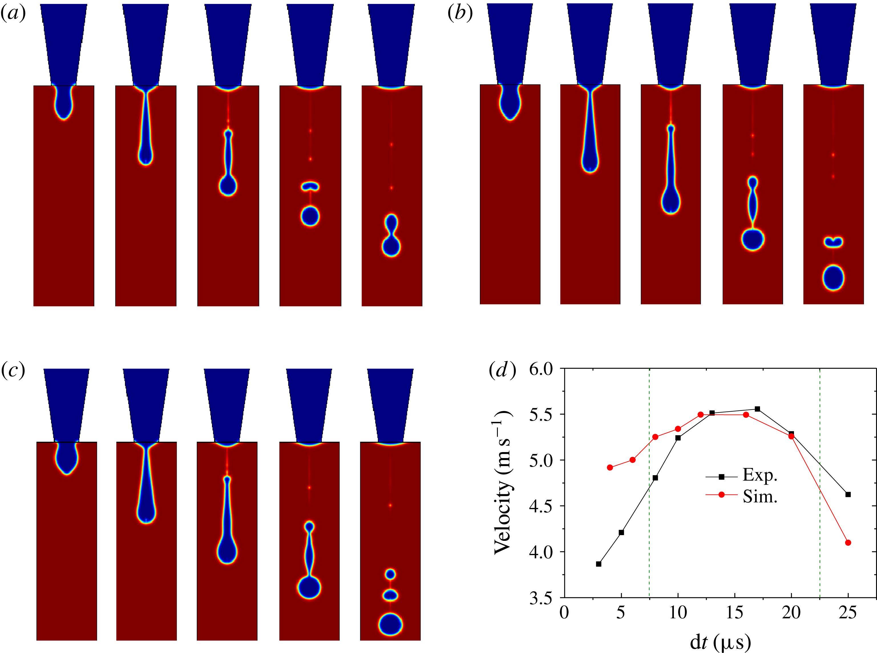
Figure 4 illustrates the influence of the pulse width on droplet ejection. The shape of the ejected droplet is greatly influenced by the pulse width. From figure 4(a), the elongated droplet breaks into a satellite droplet and a primary droplet. Then, the two droplets merge into one droplet again. However, as the pulse width increases from
 $6$
to
 $12~\unicode[STIX]{x03BC}\text{s}$
, as shown in figure 4(a–c), after the initial droplet breaks up, the number of satellites formed increases, and no merging of the droplets occurs. Figure 4(d) shows the droplet speed after leaving the nozzle. One can find that the experimental measurements and simulation results agree well with each other, which further validates the simulation models. The droplet speed increases until reaching a maximum value of approximately
 $5.5~\text{m}~\text{s}^{-1}$
for a pulse width of
 $15~\unicode[STIX]{x03BC}\text{s}$
. Then, the droplet speed decreases dramatically. The data show a significant difference in the measured and calculated speeds when the pulse width is outside of the range
 $7.5{-}22.5~\unicode[STIX]{x03BC}\text{s}$
. In practice, the hydrophilic identity of the nozzle material (glass in the experiment) may draw liquid back into the nozzle, which may further explain the discrepancy for the velocity in experiments and simulations. As shown by the experimental results, the pulse frequency has a negligible impact on droplet behaviour in the frequency range of 500–1500 Hz.
The jetting process with a nozzle diameter of (a)
 $60~\unicode[STIX]{x03BC}\text{m}$
, (b)
 $70~\unicode[STIX]{x03BC}\text{m}$
and (c)
 $80~\unicode[STIX]{x03BC}\text{m}$
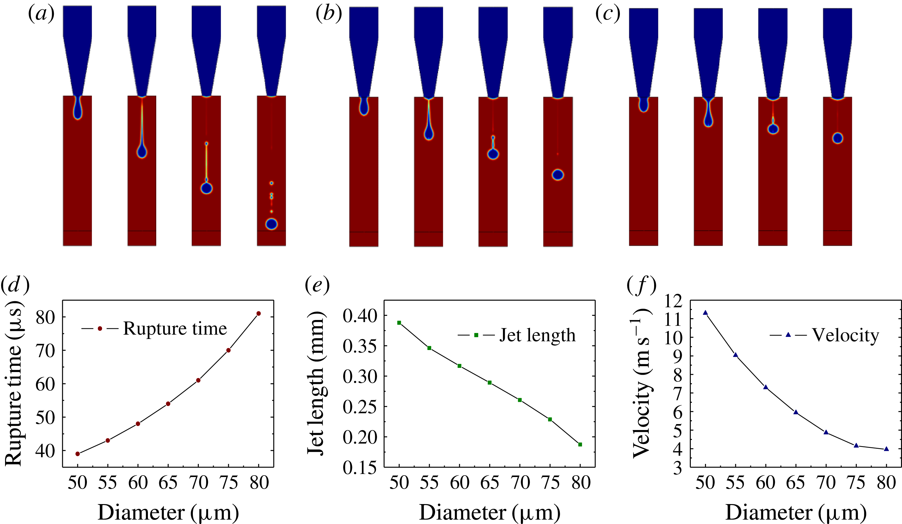
. The characteristic parameter at the rupture moment: (d) the rupture time, (e) the jet length and (f) the droplet velocity.
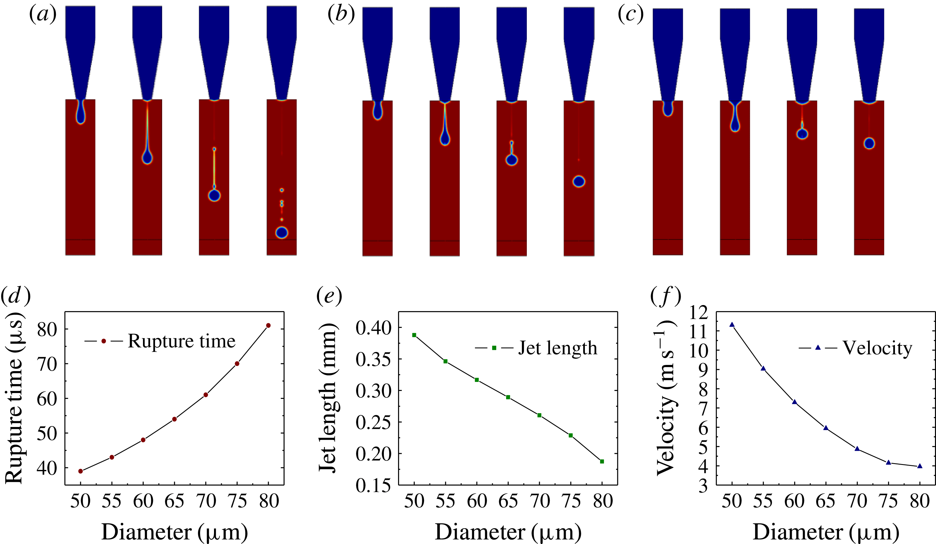
Figure 5 shows the ejected droplets for varying nozzle diameter. The time interval is
 $40~\unicode[STIX]{x03BC}\text{s}$
. The nozzle dimension is a key factor in determining the droplet size and ejection velocity. When the diameter is
 $60~\unicode[STIX]{x03BC}\text{m}$
(the minimum in this study), the ejected droplet shows a long tail. This tail gets shorter as the diameter increases. The rupture time, defined as the moment when the droplet detaches from the nozzle, increases as the diameter becomes larger. The tendency of the jet length, as defined in figure 2(c), is predicted to decrease with nozzle diameter. Similar behaviour is found for the influence of the nozzle diameter on the droplet velocity, which is defined as the velocity of the droplet when it detaches from the nozzle measured at the rupture point. Through analysis, it is found that the droplet moving velocity remains almost the same from the nozzle to the substrate since the distance between the nozzle and the substrate is not long enough to accelerate the droplet under gravity. Hence, the velocity at the rupture point is used to represent the droplet speed after ejection. From the above analysis, it is clear that the stability of the droplet can be improved using large-diameter nozzles.
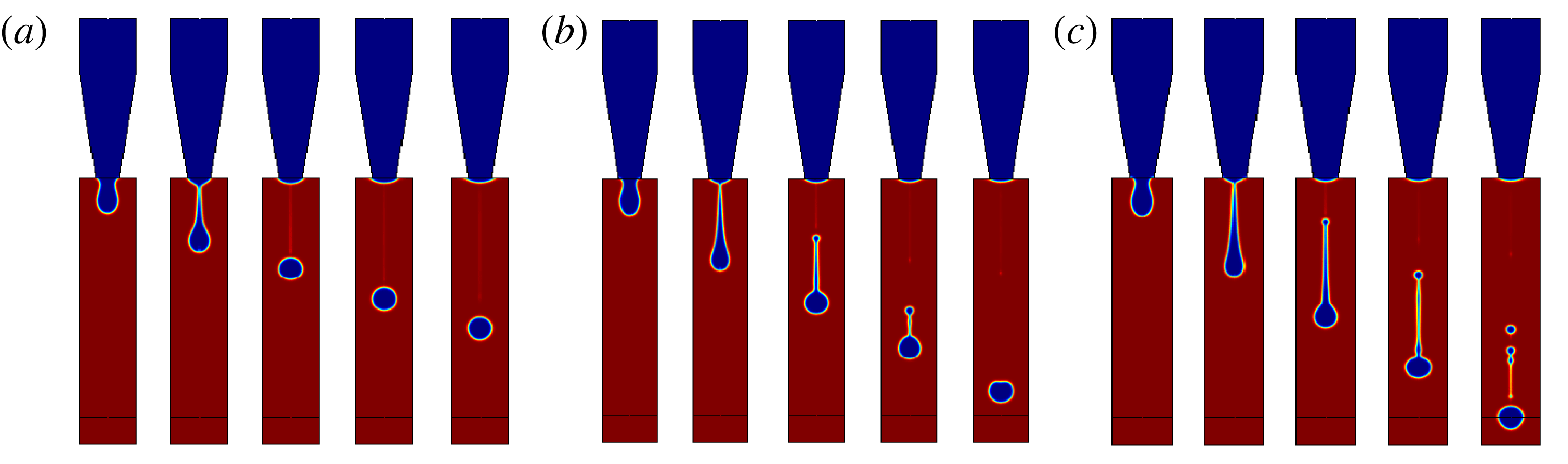
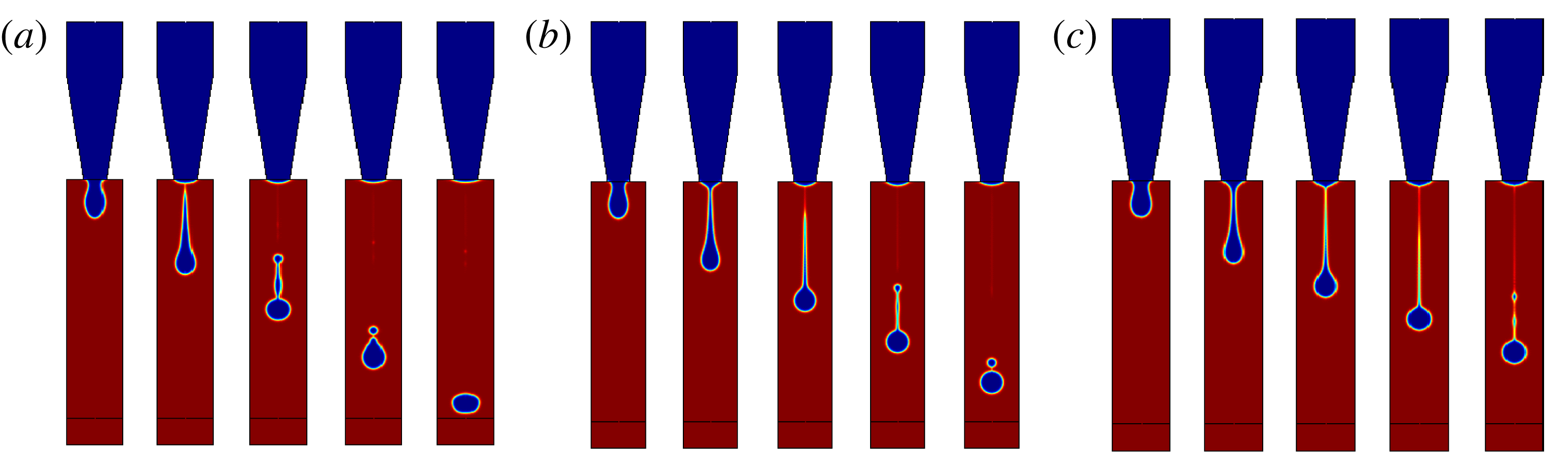
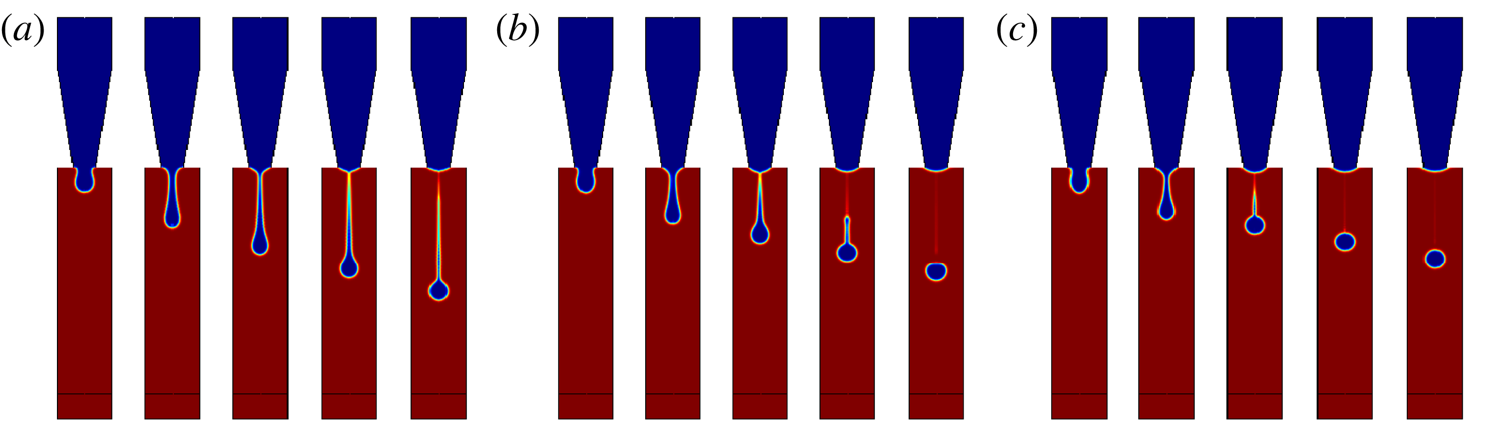
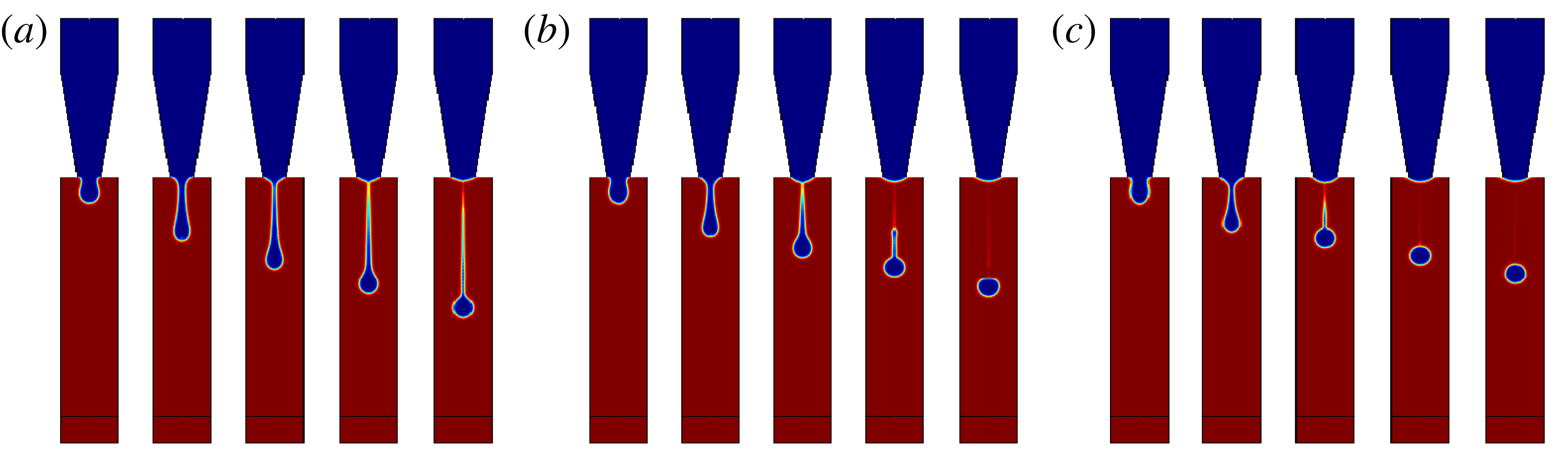
The influence of the ink/fluid properties, such as density, viscosity and surface tension, on the ejection process is shown in figures 6–8. The tail of the ejected droplet becomes longer, and the number of satellite droplets increases, for increasing density. The stability of the ejection process decreases as the density gets larger (see figure 6). Although in real experiments the density variation has no direct influence on the droplet ejection, it does affect the acoustic velocity and volume elastic modulus, both of which are related to the waveform and amplitude of the driving force. Figure 7 shows the influence of the ink viscosities on the ejection process. The increased viscous force, therefore, slows down the droplet detachment and movement, which is favourable for a stable droplet. It is noted that the viscosity effect causes a viscous loss at the nozzle and requires more energy from the pressure pulse to generate the droplets with a certain velocity. Figure 8 illustrates the influence of surface tension on the ejection process. Surface tension is a key factor affecting the shape of the initial droplet and the deformation of the primary droplet and satellite droplets. As the surface tension is set to a large value, the tail of the droplet becomes mostly invisible, and the primary droplet turns around. It is noteworthy that the surface tension also depends on the wetting characteristics between the fluid and the nozzle, which play a role in droplet reproducibility. In summary, inks with small density, large viscosity and large surface tension are preferred from the viewpoint of droplet stability.
Influence of the ink density on the ejection process. The liquid densities are (a)
 $500~\text{kg}~\text{m}^{-3}$
, (b)
 $1000~\text{kg}~\text{m}^{-3}$
and (c)
 $1500~\text{kg}~\text{m}^{-3}$
.

Influence of the ink viscosity on the ejection process. The viscosities are (a) 5 cP, (b) 15 cP and (c) 25 cP.
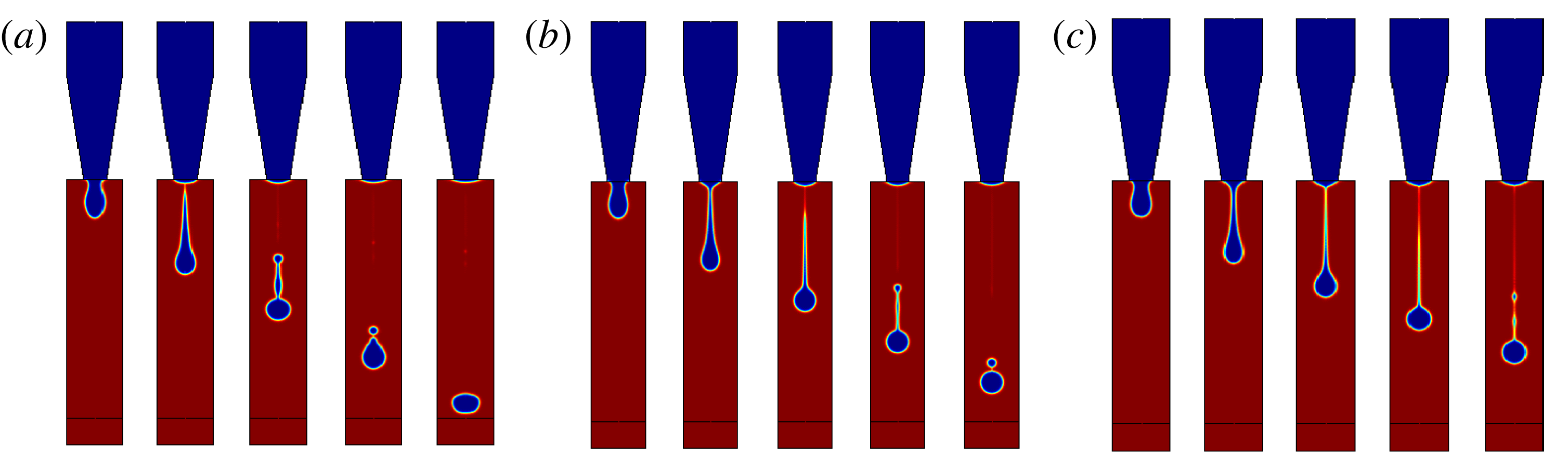
Influence of surface tension on the ejection process. The surface tensions are (a)
 $0.02~\text{N}~\text{m}^{-1}$
, (b)
 $0.04~\text{N}~\text{m}^{-1}$
and (c)
 $0.06~\text{N}~\text{m}^{-1}$
.
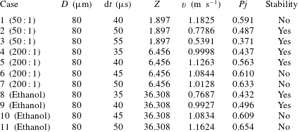
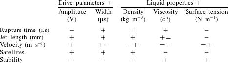
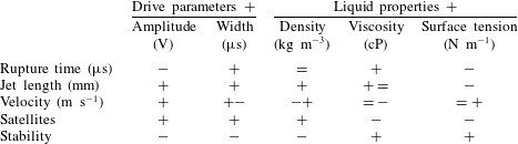
As discussed above, the droplet behaviour can be characterized in terms of the droplet parameters, i.e. the rupture time, jet length and droplet velocity. The number of satellite droplets is an intuitive description for evaluation of the stability of the ejected droplet. A summary of the operating parameters, including the droplet parameter and the ink properties, is listed in table 1. In the table, the symbols of ‘
 $+$
’, ‘
 $-$
’ and ‘
 $=$
’ represent ‘increase’, ‘decrease’ and ‘almost constant’, respectively. Two successive symbols denote a continuous change in the parameters, for example, ‘
 $+-$
’ indicates an increase followed by a decrease. From the data in the table, one can conclude that an increase in pulse amplitude, pulse width and liquid density is detrimental for achieving stable droplets. However, the coupled influence of the parameters cannot be obtained from the above analysis. As one can see from the table, the droplet parameters are influenced by the driving parameter and liquid properties in a complex manner. Since counting satellites or observing the characteristics of droplet motion is repetitive and excessive for the determination of droplet stability, it is necessary to adopt an effective and convenient criterion to prejudge whether or not the operating parameters are favourable for obtaining a stable droplet.
Variations of the droplet parameters affected by the drive parameters and liquid properties.
4.2 Stability analysis
The most popular criterion for stability analysis is based on non-dimensional parameters that combine fluid properties and droplet features. The capillary number (
 $Ca$
) represents the relative strength between the viscous force and surface tension force, the Weber number (
 $We$
) is a balance between the inertial and capillary forces and the Ohnesorge number (
 $Oh$
) relates the viscous forces to the inertial and surface tension forces. The numbers can be written as
 $$\begin{eqnarray}\displaystyle & \displaystyle Ca=\frac{v\unicode[STIX]{x1D707}}{\unicode[STIX]{x1D70E}}, & \displaystyle\end{eqnarray}$$
 $$\begin{eqnarray}\displaystyle & \displaystyle We=\frac{\unicode[STIX]{x1D70C}v^{2}l}{\unicode[STIX]{x1D70E}}, & \displaystyle\end{eqnarray}$$
 $$\begin{eqnarray}\displaystyle & \displaystyle Oh=\frac{\unicode[STIX]{x1D707}}{\sqrt{\unicode[STIX]{x1D70C}\unicode[STIX]{x1D70E}l}}, & \displaystyle\end{eqnarray}$$
where
 $v$
,
 $\unicode[STIX]{x1D707}$
,
 $\unicode[STIX]{x1D70E}$
,
 $\unicode[STIX]{x1D70C}$
and
 $l$
are the velocity, dynamic viscosity, surface tension, density and characteristic length, respectively. Here, the nozzle diameter
 $D$
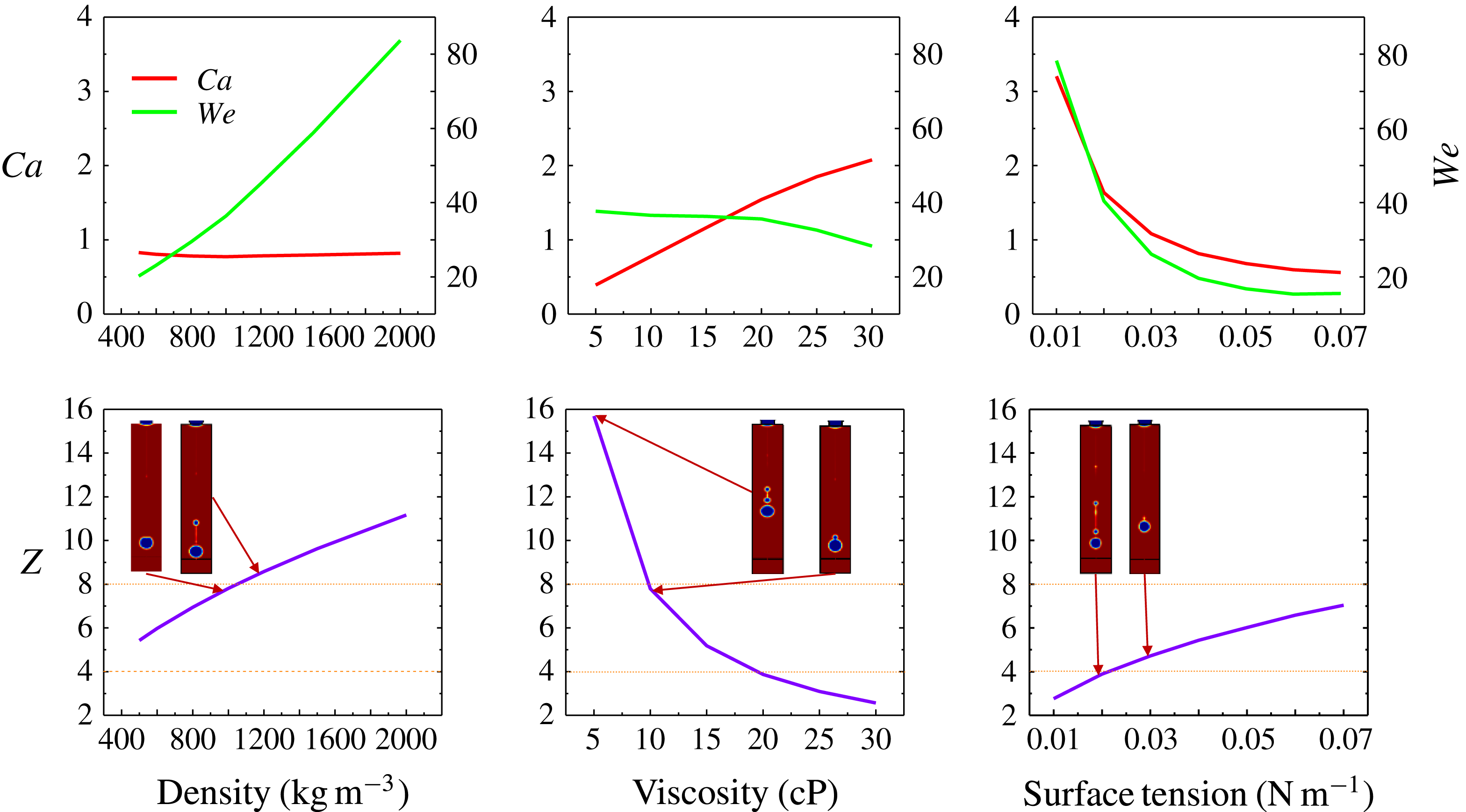
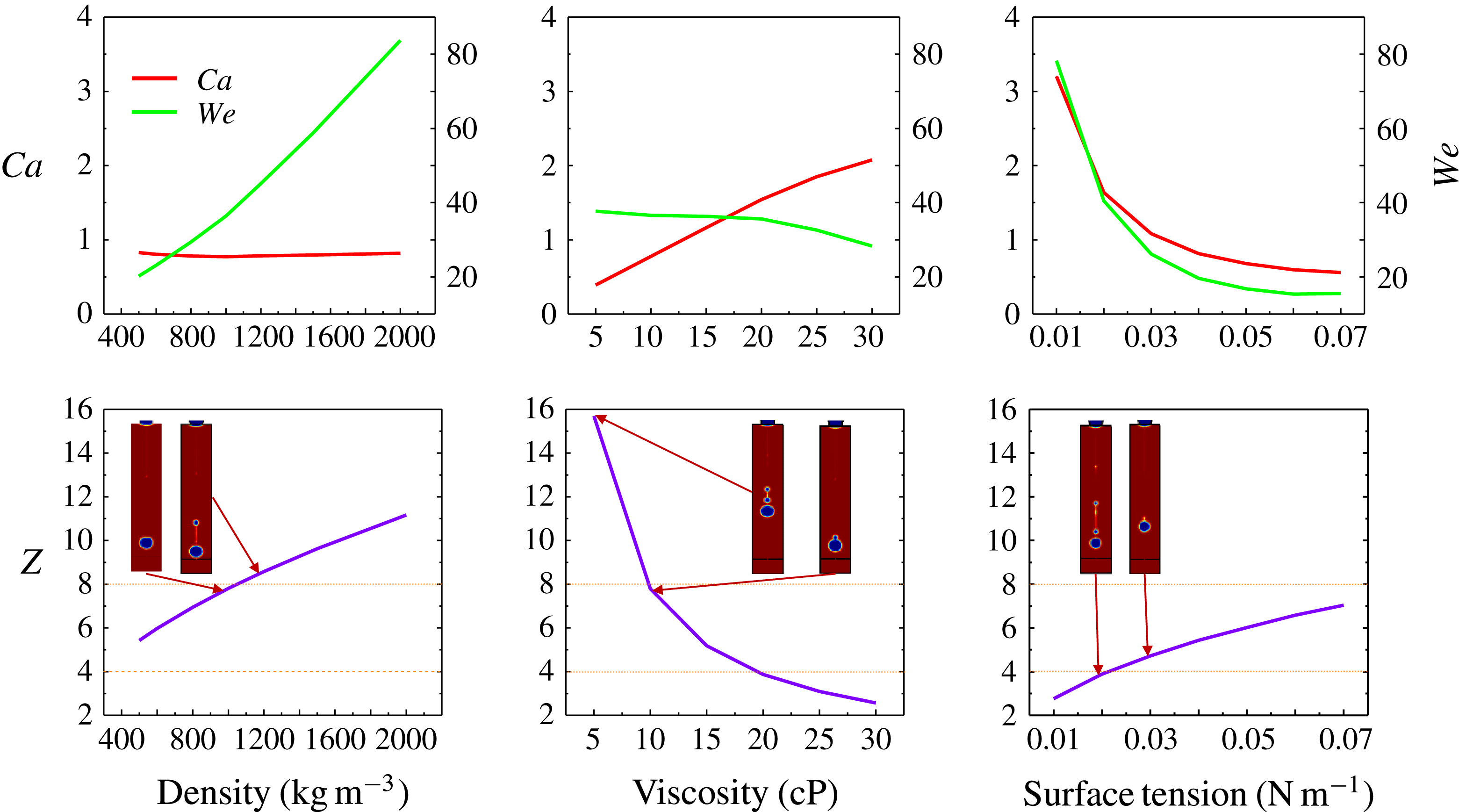
is used as the characteristic length. Figure 9 shows the dependence of the three parameters on the ink properties, including density, viscosity and surface tension.
 $Ca$
remains almost unchanged while
 $We$
increases largely for increasing density. As viscosity increases,
 $Ca$
increases significantly, while
 $We$
decreases a little for large viscosity dissipation. Both
 $Ca$
and
 $We$
clearly decrease when the surface tension increases. For stability analysis, the reciprocal of the
 $Oh$
number (
 $Z$
), is adopted. An approximate range of
 $Z$
values for a stable droplet ejection is determined to be
 $4<Z<8$
, as given in figure 9, according to numerical observations. Stable and unstable images are drawn near the critical dash line in the figure. It is noted that a primary droplet with two or more satellite droplets, or one clear satellite droplet that remains separated during movement, is considered to be unstable.
Non-dimensional parameters as a function of the fluid properties.
The ejection behaviour of the droplet, however, is dependent not only on the fluid properties but also on the operating conditions. The parameter,
 $Z$
, only considers the droplet properties explicitly unaffected by the driving conditions. Thus, a new non-dimensional parameter is introduced as a criterion to evaluate the influence of the driving parameter on droplet stability. The number is written as
 $$\begin{eqnarray}Pj=v\ast \frac{\text{d}t}{D},\end{eqnarray}$$
where
 $v$
is the droplet velocity,
 $\text{d}t$
is the pulse width and
 $D$
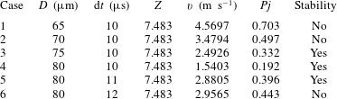
is the nozzle diameter. Since the numerical solutions were demonstrated to be accurate in the simulation of the droplet ejection process, many cases were further studied using different fluid properties and operating conditions. The cases with a stable droplet are used for calculation of the
 $Pj$
and
 $Z$
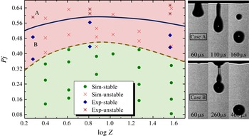
numbers. All the stable or unstable cases are denoted in figure 10 with the coordinates
 $Pj$
and
 $\log Z$
(
 $\log _{10}Z$
). As the printable range is extended to
 $1.6\leqslant Z\leqslant 40$
, which can be realized by controlling the operating conditions (Choi et al.
Reference Choi, Kim, Lee, Lee and Kim2015),
 $\log Z$
is used to make the data distribution along the
 $x$
-axis more compact. The red and green regions contain the simulated unstable and stable droplets, respectively. The boundary between the stable and unstable regions is a convex curve with a maximum value of approximately 0.44. For a given fluid with a certain
 $Z$
value, the driving parameter and the nozzle size (
 $Pj$
) can be adjusted to generate a stable droplet. The universality of
 $Pj$
is further verified by changing
 $D$
for a constant
 $\text{d}t$
and changing
 $\text{d}t$
for a constant
 $D$
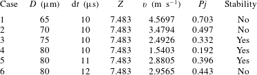
, with details shown in table 2 of the Appendix. The verification of
 $Pj$
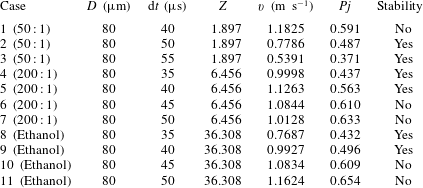
by experiment was carried out using three different liquids: ethanol, mixture 1 (ethanol and glycerol with a ratio of 50 : 1) and mixture 2 (ethanol and glycerol mixed together in a ratio of 200 : 1). Details for these experiments are given in table 3 of the Appendix. Stable and unstable points are shown in figure 10. The trend for
 $Pj$
with
 $\log Z$
is the same as that found from simulation, which verifies the reliability of the
 $Pj$
criterion. However, the overall values for
 $Pj$
from the experiments are approximately 0.16 larger than those from simulation, which may be due to viscosity dissipation and surface wettability of the nozzle, which is not exactly considered in the modelling as in the experiments. Accordingly, for a given nozzle and driving parameters, appropriate fluids can be chosen for experiments using the criterion in figure 10 as a practical guide.
Stability criterion for droplet ejection.

5 Conclusions
Inkjet technology is a fundamental technology for many applications. The droplet stability influences inkjet performance. In this paper, the stability of the droplet was numerically and experimentally analysed under different operating conditions. The results indicate that the droplet stability can be improved by decreasing the pulse amplitude and width, decreasing the fluid density and viscosity or increasing the nozzle diameter and fluid surface tension. To investigate the effect of the operating parameters on the droplet stability more completely, a new non-dimensional parameter,
 $Pj$
, is proposed as a stability criterion. Coupled with the reciprocal of the well-known Ohnesorge number (
 $Z$
), a general rule for choosing appropriate driving parameters for stable droplet ejection is illustrated in figure 10. The unstable and stable regions are clearly shown to be useful for determining experimental operating conditions for the generation of stable droplets during the inkjet process.
Acknowledgements
This work is supported by grants from the National Key Research and Development Program of China (2016YFB0303801).
Appendix
Numerical cases for varying
 $D$
for constant
 $\text{d}t$
and varying
 $\text{d}t$
for constant
 $D$
.
Experimental details for the verification points in figure 10 (liquid ratio
 $=$
ethanol : glycerol).