1 Introduction
Suspended particles in a carrier fluid can promote heat and mass transfer, catalytic chemical reactions or combustion. The dynamics of such flows is significantly more complex than single-phase flows and it is challenging to obtain a physical understanding of the phenomena at play. A particular feature of particle-laden gas flows is the tendency of inertial particles to form clusters many times larger than the particle size. To understand the mechanisms leading to clustering in semi-dilute (low volume fraction,
 $\langle \unicode[STIX]{x1D719}\rangle \ll 1$
, but moderate mass loading,
 $M=O(1)$
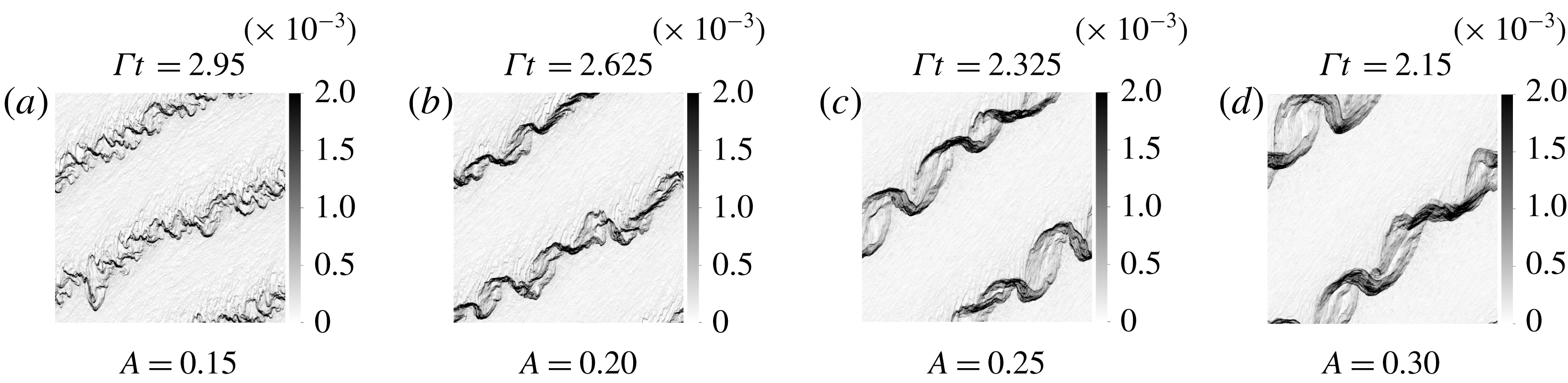
) suspensions of heavy particles in a gas, we study the case of homogeneously sheared flow. In this configuration, elongated particle clusters are continuously formed and broken down under the combined action of shear, gravity and the preferential concentration of particles in high strain and low vorticity regions of the flow. Kasbaoui et al. (Reference Kasbaoui, Koch, Subramanian and Desjardins2015) previously addressed the onset of clustering of heavy particles with small but non-zero inertia with a linear stability analysis. The nonlinear regime is addressed in this paper and reveals a route to clustering in which preferential concentration, flow modulation, particle-trajectory crossing and the Rayleigh–Taylor instability appear successively.
Semi-dilute particle-laden flow pose special challenges to physical understanding. The interplay between the two phases leads to behaviours distinctly different from purely hydrodynamic or granular flows. Most prominently, the interaction between the two phases leads to the formation of clusters in the particle phase (Squires & Eaton Reference Squires and Eaton1991; Boivin, Simonin & Squires Reference Boivin, Simonin and Squires1998; Yang & Shy Reference Yang and Shy2005; Poelma, Westerweel & Ooms Reference Poelma, Westerweel and Ooms2007; Jenny, Roekaerts & Beishuizen Reference Jenny, Roekaerts and Beishuizen2012; Meyer Reference Meyer2012; Capecelatro, Desjardins & Fox Reference Capecelatro, Desjardins and Fox2015). The aggregates of particles modulate the carrier phase on scales larger than a single particle. In turbulence, the inter-phase coupling leads to deviations of the energy and dissipation rate spectra from those predicted by the usual cascade of energy from large to small scales (Al Taweel & Landau Reference Al Taweel and Landau1977; Druzhinin Reference Druzhinin2001; Aliseda et al. Reference Aliseda, Cartellier, Hainaux and Lasheras2002; Pai & Subramaniam Reference Pai and Subramaniam2012). For heavy particles in a carrier gas, this altered energy cascade occurs even in semi-dilute suspensions and is promoted by gravity (Elghobashi & Truesdell Reference Elghobashi and Truesdell1993). Instabilities that lead to clustering of sedimenting particles could provide a mechanism by which gravitational potential energy is transformed into fluid and particle kinetic energy at length scales governed by the two-phase dynamics.
The analysis of clustering in unbounded homogeneous shear reveals mechanisms that can be hard to detect in turbulent flows. This flow retains the simplicity of linear flows but incorporates key elements of more complex anisotropic inhomogeneous flows. The seemingly simple flow exhibits singularly rich behaviours when perturbed sinusoidally and forced by gravity. In the absence of particles, Lord Kelvin (Thomson Reference Thomson1887) showed that these perturbations are diffused by the fluid’s viscosity, yielding an exponentially stable state. Recently, we showed by means of a linear stability analysis (LSA) that the addition of particles creates an unstable state through the preferential concentration mechanism (Kasbaoui et al. Reference Kasbaoui, Koch, Subramanian and Desjardins2015). The sinusoidal perturbations create periodic regions of dominant rotation and dominant strain, which cause particles to migrate and segregate breaking the homogeneity of the flow. The regions where particles accumulate force the flow in the direction of gravity more than the depleted regions do owing to the higher local number density. The overall behaviour is unstable algebraically with a time scale equal to the inverse of the shear rate. The study also reveals the existence of a most dangerous length scale, the distance travelled by a settling particle in one shear time. This most unstable wavelength is intermediate between the distance to the boundaries and the particle size. When the confining scales are much larger than this intermediate scale, the shear-driven preferential concentration instability can occur locally in a shear flow even if the shear rate and/or particle volume concentration are inhomogeneous at larger scales. This situation is analogous to the instability of particle concentration waves in fluidized beds which occur at a preferred wavelength governed by particle inertia, particle pressure and particle viscosity (Anderson, Sundaresan & Jackson Reference Anderson, Sundaresan and Jackson1995). In contrast the instabilities of single-phase shear flow emerge from the boundaries. The work exposes the onset of clustering in homogeneous shear flow based on a simplified Eulerian–Eulerian model first proposed by Maxey (Reference Maxey1987) and then further developed by Druzhinin (Reference Druzhinin1995) and Ferry & Balachandar (Reference Ferry and Balachandar2001) valid for heavy particles with small, but non-zero inertia. Characterization of the full clustering route requires analysis of the flow with large perturbations out of the reach of LSA.
Experimental investigations of clustering in unbounded homogeneous shear are rendered difficult by the size of parameter space to be explored and flow geometry. In addition to the usual Reynolds number
 $Re$
, the mass loading
 $M$
(ratio of the masses of the two phases), Stokes number
 $St$
(product of shear rate and particle characteristic time) and average particle volume fraction
 $\langle \unicode[STIX]{x1D719}\rangle$
are parameters that critically dictate the working regime of particle-laden flows. Moreover, experiments are often hard to conduct because of the two phases obstructing each other (Modarress, Elghobashi & Tan Reference Modarress, Elghobashi and Tan1984; Shuen et al.
Reference Shuen, Solomon, Faeth and Zhang1985; Hardalupas, Taylor & Whitelaw Reference Hardalupas, Taylor and Whitelaw1989; Mostafa et al.
Reference Mostafa, Mongia, Mcdonel and Samuelsen1989; Prevost et al.
Reference Prevost, Boree, Nuglisch and Charnay1996; Gillandt, Fritsching & Bauckhage Reference Gillandt, Fritsching and Bauckhage2001; Yang & Shy Reference Yang and Shy2005; Poelma et al.
Reference Poelma, Westerweel and Ooms2007; Lau & Nathan Reference Lau and Nathan2014). These difficulties make numerical approaches particularly appealing in this context.
Numerical endeavours start by a choice of governing equations to be solved. There are two dominant paradigms for treating the two phases, each with their own conceptual difficulties. Euler–Lagrange (EL) simulations rely on solving the position and momentum of every discrete (Lagrangian) particle in addition to the fluid’s Navier–Stokes equations. This method is successful in capturing clustering in mesoscale simulations but cannot realistically scale to match laboratory-scale experiments, let alone industrial flows, because the number of particles to track quickly becomes intractable. An alternative formalism relies on an Eulerian description of the particle phase. Euler–Euler (EE) approaches are usually more computationally efficient and easier to scale. However, the analysis of clustering with these methods is challenging. One challenge is the conceptual difficulties in the derivation of partial differential equations (PDE) for the particle volume fraction and momentum that lead to limits to their applicability. The particle phase is highly compressible and as such particles are allowed to accumulate in restricted regions of space. The compressibility of the particle phase leads to strong volume fraction gradients, shocks and void bubbles, i.e. depleted regions where the volume fraction approaches zero. According to Ferrante & Elghobashi (Reference Ferrante and Elghobashi2007) this results in particle velocity fields that contain ‘holes’ indicating a topology change. Moreover, the dynamics of the particle often leads to local folds in phase space resulting in caustics (Falkovich, Fouxon & Stepanov Reference Falkovich, Fouxon and Stepanov2002; Wilkinson, Mehlig & Bezuglyy Reference Wilkinson, Mehlig and Bezuglyy2006; Gustavsson et al. Reference Gustavsson, Meneguz, Reeks and Mehlig2012; Ravichandran & Govindarajan Reference Ravichandran and Govindarajan2015). The ability of particles to cross one another’s trajectories leads to local multiplicity in the particle velocity (Fox Reference Fox2008). This prompted the development of kinetic models (Koch Reference Koch1990) and other approaches inspired by rarefied gas flows (McGraw Reference McGraw1997; Simonin, Fevrier & Laviville Reference Simonin, Fevrier and Laviville2002; Desjardins, Fox & Villedieu Reference Desjardins, Fox and Villedieu2008; Fox Reference Fox2008). In this exploratory work, we use leading EE and EL methods to expose similarities and differences across the methodologies.
Building on the linear analysis, we propose to revisit the instability in the light of the EL methodology (Capecelatro & Desjardins Reference Capecelatro and Desjardins2013b ) and two EE approaches: the low volume fraction two-fluid method (TF) (Elghobashi & AbouArab Reference Elghobashi and AbouArab1983; Druzhinin Reference Druzhinin1994) and the anisotropic-Gaussian method (AG) (Vi, Doisneau & Massot Reference Vi, Doisneau and Massot2015). In § 2, we present the governing equations and outlines of the instability. Section 3 presents the numerical strategies. Careful attention is given to the forcing by the homogeneous shear and the shear-periodic boundary conditions. In § 4, the numerical results are compared to the linear stability analysis in the small amplitude regime. This shows agreement across all methods when the particle distribution inhomogeneities are small. In § 5, we probe the flow with strong perturbations that trigger nonlinear effects. This leads to strong clustering in EL and EE simulations, aided by a secondary Rayleigh–Taylor instability and particle-trajectory crossing. The differences noted in the three computational approaches expose the importance of particle-trajectory crossing in removing discontinuities arising in TF simulations. Concluding remarks are reported in § 6.
2 Particle-laden homogeneous shear
2.1 Governing equations and particle-phase methods
Consider a dilute monodisperse cloud of particles suspended in an incompressible Newtonian gas. The carrier phase has a density
 $\unicode[STIX]{x1D70C}_{f}$
and viscosity
 $\unicode[STIX]{x1D707}_{f}$
and satisfies the Navier–Stokes equations
 $$\begin{eqnarray}\displaystyle & \displaystyle \unicode[STIX]{x1D735}\boldsymbol{\cdot }\boldsymbol{U}=0, & \displaystyle\end{eqnarray}$$
 $$\begin{eqnarray}\displaystyle & \displaystyle \unicode[STIX]{x1D70C}_{f}\frac{\unicode[STIX]{x2202}\boldsymbol{U}}{\unicode[STIX]{x2202}t}+\unicode[STIX]{x1D70C}_{f}\boldsymbol{U}\boldsymbol{\cdot }\unicode[STIX]{x1D735}\boldsymbol{U}=-\unicode[STIX]{x1D735}p+\unicode[STIX]{x1D707}_{f}\unicode[STIX]{x1D6FB}^{2}\boldsymbol{U}+\unicode[STIX]{x1D70C}_{f}\boldsymbol{g}-\boldsymbol{F}, & \displaystyle\end{eqnarray}$$
where
 $\boldsymbol{U}$
is the fluid velocity,
 $p$
is the pressure,
 $\boldsymbol{g}$
is the gravitational acceleration and
 $\boldsymbol{F}$
is the momentum coupling force with the dispersed phase. For dilute solid particles of density
 $\unicode[STIX]{x1D70C}_{p}$
, diameter
 $d_{p}$
, velocity
 $\boldsymbol{V}$
, relaxation time
 $\unicode[STIX]{x1D70F}_{p}=\unicode[STIX]{x1D70C}_{p}d_{p}^{2}/(18\unicode[STIX]{x1D707}_{f})$
, with diameters small enough that the particle Reynolds number
 $Re_{p}=|v-u|d_{p}/\unicode[STIX]{x1D708}<1$
(Maxey & Riley Reference Maxey and Riley1983), this coupling is captured by the Stokes drag
 $$\begin{eqnarray}\boldsymbol{F}=\unicode[STIX]{x1D70C}_{p}\unicode[STIX]{x1D719}\frac{\boldsymbol{U}-\boldsymbol{V}}{\unicode[STIX]{x1D70F}_{p}},\end{eqnarray}$$
where
 $\unicode[STIX]{x1D719}$
is the local volume fraction. The remaining hydrodynamic forces are neglected. Note that the gravitational force acting on the particles does not directly force the fluid motion. Instead, the gravitational force alters the particle velocity in a way that leads to a particle–fluid drag force (2.3) that resembles gravitational loading when the difference of velocities is nearly relaxed to the terminal velocity at low Stokes numbers.
It is important to note that semi-dilute suspensions for which the average volume fraction
 $\langle \unicode[STIX]{x1D719}\rangle$
is small can still have a strong coupling between the two phases. Owing to the large density ratio
 $\unicode[STIX]{x1D70C}_{p}/\unicode[STIX]{x1D70C}_{f}$
of solid particles in gaseous flows, the mass loading
 $M=\langle \unicode[STIX]{x1D719}\rangle \unicode[STIX]{x1D70C}_{p}/\unicode[STIX]{x1D70C}_{f}$
, a measure of the coupling between the phases, can be of order unity. This means ensembles of particles can collectively modulate the flow on a level on par with the mean fluid velocity.
When treating homogeneous shear flows, it is customary to do a decomposition that isolates the perturbations from the mean homogeneous shear motion
 $$\begin{eqnarray}\displaystyle & \displaystyle \boldsymbol{U}=\unicode[STIX]{x1D6E4}y\boldsymbol{e}_{x}+\boldsymbol{u}, & \displaystyle\end{eqnarray}$$
 $$\begin{eqnarray}\displaystyle & \displaystyle \boldsymbol{V}=\unicode[STIX]{x1D6E4}y\boldsymbol{e}_{x}+\boldsymbol{v}. & \displaystyle\end{eqnarray}$$
Here
 $\boldsymbol{u}$
and
 $\boldsymbol{v}$
are the fluctuating fluid and particle velocities,
 $\unicode[STIX]{x1D6E4}$
is the shear rate,
 $\boldsymbol{e}_{x}$
is the streamwise direction and
 $y$
is the coordinate along the cross-direction
 $\boldsymbol{e}_{y}=-\boldsymbol{g}/g$
which is also parallel to gravity. The fluid fluctuations are given by the following governing equations:
 $$\begin{eqnarray}\displaystyle & \displaystyle \unicode[STIX]{x1D735}\boldsymbol{\cdot }\boldsymbol{u}=0, & \displaystyle\end{eqnarray}$$
 $$\begin{eqnarray}\displaystyle & \displaystyle \unicode[STIX]{x1D70C}_{f}\frac{\unicode[STIX]{x2202}\boldsymbol{u}}{\unicode[STIX]{x2202}t}+\unicode[STIX]{x1D70C}_{f}\boldsymbol{u}\boldsymbol{\cdot }\unicode[STIX]{x1D735}\boldsymbol{u}=-\unicode[STIX]{x1D735}p+\unicode[STIX]{x1D707}_{f}\unicode[STIX]{x1D6FB}^{2}\boldsymbol{U}+\unicode[STIX]{x1D70C}_{f}\boldsymbol{g}-\boldsymbol{F}-\unicode[STIX]{x1D70C}_{f}\unicode[STIX]{x1D6E4}u_{y}\boldsymbol{e}_{x}-\unicode[STIX]{x1D70C}_{f}\unicode[STIX]{x1D6E4}y\frac{\unicode[STIX]{x2202}\boldsymbol{u}}{\unicode[STIX]{x2202}x}. & \displaystyle\end{eqnarray}$$
In the absence of particles, the homogeneous shear flow contains only two intrinsic scales: the shear characteristic time
 $\unicode[STIX]{x1D70F}_{f}=\unicode[STIX]{x1D6E4}^{-1}$
, and the shear viscous dissipation length scale
 $L_{\unicode[STIX]{x1D707}}=\sqrt{\unicode[STIX]{x1D707}_{f}/(\unicode[STIX]{x1D70C}_{f}\unicode[STIX]{x1D6E4})}$
. The unboundedness of the flow removes any other scale. New scales arise in particle-laden shear subject to gravity. As explained in Kasbaoui et al. (Reference Kasbaoui, Koch, Subramanian and Desjardins2015), the unperturbed sheared particle-phase sediments at the speed of the particle settling velocity
 $V_{g}=\unicode[STIX]{x1D70F}_{p}g$
. Based on this characteristic velocity and the characteristic time
 $\unicode[STIX]{x1D70F}_{f}=\unicode[STIX]{x1D6E4}^{-1}$
, non-dimensionalization of the two-fluid equations reveals a characteristic length equal to the settling distance in one shear time,
 $L_{g}=V_{g}/\unicode[STIX]{x1D6E4}$
. This is a scaling that focuses on the collective dynamics of the particles in shear, rather than the particle-scale dynamics. It follows that a total of four independent dimensionless numbers control this flow: the mass loading
 $M$
, average volume fraction
 $\langle \unicode[STIX]{x1D719}\rangle$
, Stokes number
 $St=\unicode[STIX]{x1D6E4}\unicode[STIX]{x1D70F}_{p}$
and Reynolds number
 $Re=\unicode[STIX]{x1D70C}_{f}V_{g}L_{g}/\unicode[STIX]{x1D707}_{f}=(L_{g}/L_{\unicode[STIX]{x1D707}})^{2}$
. In this context, the Reynolds number is a measure of the relative strength of inertial accelerations at the scale set by the particles’ sedimentation to the viscous dissipation. It also shows that fluid perturbations induced by slow settling particles are suppressed by viscosity. It is noteworthy that, while shear reinforces preferential concentration (Kasbaoui et al.
Reference Kasbaoui, Koch, Subramanian and Desjardins2015), it can also lead to reduced flow modulation by strengthening the dissipation compared to the gravitational effects (
 $Re=(L_{g}/L_{\unicode[STIX]{x1D707}})^{2}\propto 1/\unicode[STIX]{x1D6E4}$
).
A complete description of particle-laden flows requires governing equations for the particle phase. Below we examine three approaches used in the present study.
Euler–Lagrange method (EL): Based on the work of Maxey & Riley (Reference Maxey and Riley1983), the equation of motion of particle ‘
 $i$
’ in homogeneous shear is given by
 $$\begin{eqnarray}\displaystyle & \displaystyle \frac{\text{d}\boldsymbol{x}^{i}}{\text{d}t}=\boldsymbol{v}^{i}+\unicode[STIX]{x1D6E4}y^{i}\boldsymbol{e}_{x}, & \displaystyle\end{eqnarray}$$
 $$\begin{eqnarray}\displaystyle & \displaystyle \frac{\text{d}\boldsymbol{v}^{i}}{\text{d}t}=\frac{\boldsymbol{u}(\boldsymbol{x}^{i},t)-\boldsymbol{v}^{i}}{\unicode[STIX]{x1D70F}_{p}}+\boldsymbol{g}, & \displaystyle\end{eqnarray}$$
where
 $\boldsymbol{x}^{i}$
and
 $\boldsymbol{v}^{i}$
are respectively the position and fluctuating velocity of this particle. Only Stokes drag is retained here for the same reasons as in (2.3).
Euler–Lagrange approaches rely on solving these equations for all
 $N$
discrete particles in the flow. The Eulerian particle velocity at the location
 $\boldsymbol{x}$
is computed from the Lagrangian velocities in the following way:
 $$\begin{eqnarray}\boldsymbol{v}(\boldsymbol{x},t)=\frac{1}{N}\mathop{\sum }_{i}^{N}v^{i}(t)q(\Vert \boldsymbol{x}-\boldsymbol{x}^{i}\Vert ),\end{eqnarray}$$
where
 $q$
is a filter kernel with width
 $\unicode[STIX]{x1D6FF}_{f}$
comparable to the grid spacing
 $\unicode[STIX]{x0394}x$
. The particle volume fraction
 $\unicode[STIX]{x1D719}$
is obtained in a similar way. The construction of these Eulerian quantities allow the evaluation of the forcing term (2.3) exerted by the particles on the gas.
Two-fluid Euler–Euler method (TF): Euler–Euler formulations derive from the observation that on scales significantly larger than the particle diameter but smaller than the confining apparatus, the particle phase bears a coherent, organized, fluid-like motion. In these approaches the Eulerian particle velocity
 $\boldsymbol{v}$
becomes the subject of models and equations to be solved. The discrete particulate view is lost in favour of a continuum description in terms of number density
 $n=\unicode[STIX]{x1D719}\unicode[STIX]{x03C0}d_{p}^{3}/6$
and particle velocity field
 $\boldsymbol{v}$
.
In two-fluid methods for semi-dilute suspensions, the population balance is dictated by pure advection by the particle velocity field. The latter is found by taking the derivative in (2.9) along the particle trajectory
 $\text{d}/\text{d}t=\unicode[STIX]{x2202}/\unicode[STIX]{x2202}t+\boldsymbol{v}\boldsymbol{\cdot }\unicode[STIX]{x1D735}$
. The governing equations for the dispersed phase have the following conservative form:
 $$\begin{eqnarray}\displaystyle & \displaystyle \frac{\unicode[STIX]{x2202}(\unicode[STIX]{x1D70C}_{p}n)}{\unicode[STIX]{x2202}t}+\unicode[STIX]{x1D735}\boldsymbol{\cdot }(\unicode[STIX]{x1D70C}_{p}n\boldsymbol{v})=-\unicode[STIX]{x1D6E4}y\frac{\unicode[STIX]{x2202}(\unicode[STIX]{x1D70C}_{p}n)}{\unicode[STIX]{x2202}x}, & \displaystyle\end{eqnarray}$$
 $$\begin{eqnarray}\displaystyle & \displaystyle \frac{\unicode[STIX]{x2202}(\unicode[STIX]{x1D70C}_{p}n\boldsymbol{v})}{\unicode[STIX]{x2202}t}+\unicode[STIX]{x1D735}\boldsymbol{\cdot }(\unicode[STIX]{x1D70C}_{p}n\boldsymbol{v}\boldsymbol{v})=\unicode[STIX]{x1D70C}_{p}n\boldsymbol{g}+\unicode[STIX]{x1D70C}_{p}n\frac{\boldsymbol{u}-\boldsymbol{v}}{\unicode[STIX]{x1D70F}_{p}}-\unicode[STIX]{x1D70C}_{p}n\unicode[STIX]{x1D6E4}v_{y}\boldsymbol{e}_{x}-\unicode[STIX]{x1D6E4}y\frac{\unicode[STIX]{x2202}(\unicode[STIX]{x1D70C}_{p}n\boldsymbol{v})}{\unicode[STIX]{x2202}x}. & \displaystyle\end{eqnarray}$$
The shear decomposition is assumed in the equations above. Together with the fluid’s mass and momentum conservation equations, equations (2.11), (2.12), (2.1) and (2.2) provide a complete set of equations to describe semi-dilute gas–solid flows.
Anisotropic-Gaussian Euler–Euler method (AG): Equation (2.12) relies on the fundamental hypothesis that the particle velocity field is single valued. This is not always true for gas–solid flows. In fact, a feature of inertial particulate flows is the ability of trajectories of particles with different histories to cross leading to multiple particle velocities at a single point. Kinetic based methods recognize this as a limitation and borrow from the rarefied-flow community to handle the crossing characteristics. The idea is to allow the particle velocity field to take multiple values, by solving a probabilistic equation governing the number density probability density function (pdf)
 $f(t,\boldsymbol{x},\boldsymbol{v})$
. Following Williams (Reference Williams1958), the equation in phase space for the pdf of a dilute system of collisionless particles interacting only through the mean fluid velocity is given by
 $$\begin{eqnarray}\frac{\unicode[STIX]{x2202}f}{\unicode[STIX]{x2202}t}+\boldsymbol{c}\boldsymbol{\cdot }\unicode[STIX]{x1D735}_{x}\,f+\unicode[STIX]{x1D735}_{c}\boldsymbol{\cdot }\left(f\left(\frac{\boldsymbol{u}-\boldsymbol{v}}{\unicode[STIX]{x1D70F}_{p}}+\boldsymbol{g}\right)\right)=0.\end{eqnarray}$$
Because of the larger space of variables, equation (2.13) is vastly more complicated to solve. To make this method computationally tractable, many methods rely on solving for a finite number of moments instead of the full pdf
 $f$
. Since the transport of every moment relies on the next-order moment, the difficulty resides in finding a closure to the high-order ones. One approach is to formulate closures in the form of constitutive relations linking high-order moments to low-order ones given in physical space. These are usually applicable for a limited range of Stokes number. See Simonin et al. (Reference Simonin, Fevrier and Laviville2002), Fvrier, Simonin & Squires (Reference Fevrier, Simonin and Squires2005) and Kaufmann et al. (Reference Kaufmann, Moreau, Simonin and Helie2008) for small Stokes number closures, and Masi & Simonin (Reference Masi and Simonin2014) for large Stokes number ones. Another approach is based on postulating a form of the number density pdf itself. With a choice of pdf using only low-order moments, the high-order moments can be found from direct integration of the pdf, hence, providing closure to the moment transport equations (Desjardins et al.
Reference Desjardins, Fox and Villedieu2008; Fox Reference Fox2008). This is the method we follow in this paper.
In this work, we focus on the anisotropic-Gaussian closure, originally proposed for rarefied gases (Levermore & Morokoff Reference Levermore and Morokoff1998) and later extended to particle-laden flows (Vi et al. Reference Vi, Doisneau and Massot2015). In this method, the number density pdf is approximated by
 $$\begin{eqnarray}f(\boldsymbol{c})=\frac{\unicode[STIX]{x1D70C}_{p}n}{(2\unicode[STIX]{x03C0}|\boldsymbol{P}_{p}|)^{2/3}}\exp \left(-\frac{1}{2}(\boldsymbol{c}-\boldsymbol{v})\boldsymbol{\cdot }\boldsymbol{P}_{p}^{-1}(\boldsymbol{c}-\boldsymbol{v})\right),\end{eqnarray}$$
where
 $\boldsymbol{v}=(\unicode[STIX]{x1D70C}_{p}n)^{-1}\int \boldsymbol{c}f\,\text{d}\boldsymbol{c}$
is the Eulerian particle velocity (first-order moment) and
 $\boldsymbol{P}_{p}$
is the particle pressure tensor derived from the energy tensor (second-order moment)
 $\boldsymbol{E}=\int \boldsymbol{c}\boldsymbol{c}f\,\text{d}\boldsymbol{c}=\unicode[STIX]{x1D70C}_{p}n(\boldsymbol{P}_{p}+\boldsymbol{v}\boldsymbol{v})$
. It is clear that moments up to the second order need to be solved in order to build the presumed AG pdf. Using the shear decomposition, these read
 $$\begin{eqnarray}\displaystyle & \displaystyle \frac{\unicode[STIX]{x2202}\unicode[STIX]{x1D70C}_{p}n}{\unicode[STIX]{x2202}t}+\unicode[STIX]{x1D735}\boldsymbol{\cdot }(\unicode[STIX]{x1D70C}_{p}n\boldsymbol{v})=-\unicode[STIX]{x1D6E4}y\frac{\unicode[STIX]{x2202}\unicode[STIX]{x1D70C}_{p}n}{\unicode[STIX]{x2202}x}, & \displaystyle\end{eqnarray}$$
 $$\begin{eqnarray}\displaystyle & \displaystyle \frac{\unicode[STIX]{x2202}(\unicode[STIX]{x1D70C}_{p}n\boldsymbol{v})}{\unicode[STIX]{x2202}t}+\unicode[STIX]{x1D735}\boldsymbol{\cdot }\boldsymbol{E}=\unicode[STIX]{x1D70C}_{p}n\boldsymbol{g}+\frac{\unicode[STIX]{x1D70C}_{p}n\boldsymbol{u}-(\unicode[STIX]{x1D70C}_{p}n\boldsymbol{v})}{\unicode[STIX]{x1D70F}_{p}}-\unicode[STIX]{x1D70C}_{p}n\unicode[STIX]{x1D6E4}v_{y}\boldsymbol{e}_{x}-\unicode[STIX]{x1D6E4}y\frac{\unicode[STIX]{x2202}(\unicode[STIX]{x1D70C}_{p}n\boldsymbol{v})}{\unicode[STIX]{x2202}x}, & \displaystyle\end{eqnarray}$$
 $$\begin{eqnarray}\displaystyle \frac{\unicode[STIX]{x2202}\boldsymbol{E}}{\unicode[STIX]{x2202}t}+\unicode[STIX]{x1D735}\boldsymbol{\cdot }\boldsymbol{Q} & = & \displaystyle \boldsymbol{g}(\unicode[STIX]{x1D70C}_{p}n\boldsymbol{v})+(\unicode[STIX]{x1D70C}_{p}n\boldsymbol{v})\boldsymbol{g}+\frac{(\unicode[STIX]{x1D70C}_{p}n\boldsymbol{v})\boldsymbol{u}+\boldsymbol{u}(\unicode[STIX]{x1D70C}_{p}n\boldsymbol{v})-2\boldsymbol{E}}{\unicode[STIX]{x1D70F}_{p}}\nonumber\\ \displaystyle & & \displaystyle -\,\unicode[STIX]{x1D6E4}(\boldsymbol{E}\boldsymbol{\cdot }\boldsymbol{e}_{\boldsymbol{y}})\boldsymbol{e}_{x}-\unicode[STIX]{x1D6E4}\boldsymbol{e}_{x}(\boldsymbol{e}_{y}\boldsymbol{\cdot }\boldsymbol{E})-\unicode[STIX]{x1D6E4}y\frac{\unicode[STIX]{x2202}\boldsymbol{E}}{\unicode[STIX]{x2202}x},\end{eqnarray}$$
where
 $\boldsymbol{Q}$
is the particle heat flux third-order tensor, a third-order moment that requires closure. The reconstruction of the AG distribution provides closure by allowing the direct computation of this moment from the presumed pdf
 $\boldsymbol{Q}=\int \boldsymbol{c}\boldsymbol{c}\boldsymbol{c}f\,\text{d}\boldsymbol{c}$
.
Sabat et al. (Reference Sabat, Vié, Larat and Massot2016) show that the AG method reproduces the same level of clustering found in Euler–Lagrange simulations of one-way coupled decaying homogeneous isotropic turbulence. The agreement holds across the whole range of Stokes number in contrast to the TF method which leads to excessive clustering for moderate and large Stokes numbers. The success of this approach stems from its ability to capture the particle dispersion due to particle-trajectory crossing. It is also argued to be the most likely distribution, in the sense of entropy maximization, given the moments of
 $f$
up to the second order (Vi et al.
Reference Vi, Doisneau and Massot2015).
Note that the AG method can be considered as an extension of the TF method. In the limit of infinitely small Stokes number, the particle pressure tensor vanishes and the AG distribution collapses onto the mono-kinetic distribution
 $f(t,\boldsymbol{x},\boldsymbol{c})=n(t,\boldsymbol{x})\unicode[STIX]{x1D6FF}(\boldsymbol{c}-\boldsymbol{v}(t,\boldsymbol{x}))$
. Integrating the moments of the population balance equation (2.13) with this distribution yields the TF equations (2.11) and (2.12).
To conclude this section, we shall note that many (Druzhinin Reference Druzhinin1995; Ferry & Balachandar Reference Ferry and Balachandar2001; Vi et al.
Reference Vi, Doisneau and Massot2015) have argued, based on one-way coupling studies, that particle trajectory crossing for flows with small volume fraction and small Stokes number is negligible. However, this has not been verified in the two-way coupled semi-dilute regime. In the following, the granular temperature
 $\unicode[STIX]{x1D6E9}=\text{Tr}(\boldsymbol{P}_{p})/3$
from the AG and EL methods will serve as a measure of the presence of trajectory crossing as this quantity is identically zero in the TF method.
2.2 An algebraic instability
The instability of particle-laden shear is the result of two concomitant effects: preferential concentration and an inertial acceleration or gravity. It is possible to show that preferential concentration is directly related to the extreme compressibility of the particle phase (Maxey Reference Maxey1987). For particles with small inertia, the rate of volumetric expansion and contraction is given by
 $$\begin{eqnarray}\unicode[STIX]{x1D735}\boldsymbol{\cdot }\boldsymbol{v}\simeq \unicode[STIX]{x1D70F}_{p}(S-R)+O(\unicode[STIX]{x1D70F}_{p}^{2}),\end{eqnarray}$$
where
 $S=1/2(\unicode[STIX]{x1D735}\boldsymbol{u}+\unicode[STIX]{x1D735}\boldsymbol{u}^{\text{T}}):1/2(\unicode[STIX]{x1D735}\boldsymbol{u}+\unicode[STIX]{x1D735}\boldsymbol{u}^{\text{T}})$
and
 $R=1/2(\unicode[STIX]{x1D735}\boldsymbol{u}-\unicode[STIX]{x1D735}\boldsymbol{u}^{\text{T}}):1/2(\unicode[STIX]{x1D735}\boldsymbol{u}-\unicode[STIX]{x1D735}\boldsymbol{u}^{\text{T}})$
denote the second invariants of the fluid strain and rotation tensors (Squires & Eaton Reference Squires and Eaton1991). When the local strain exceeds the local rotation particles accumulate. In the opposite scenario of local rotation dominating over strain, the particles are expelled. In pure particle-laden homogeneous shear, strain and rotation perfectly balance each other
 $S=R=\unicode[STIX]{x1D6E4}/2$
leading to no preferential concentration. Additionally, a cloud of homogeneously distributed particles exerts a uniform gravitational loading on the fluid, the effect of which is an increased hydrostatic pressure. This state is possible but not tenable as minute perturbations quickly alter these balances.
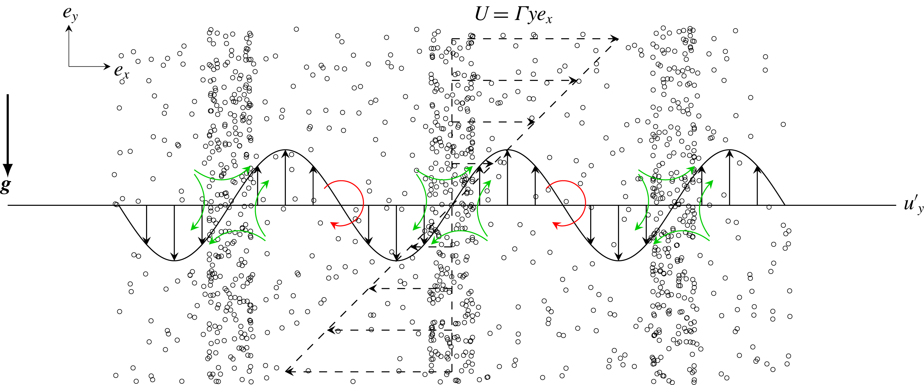
Figure 1 illustrates the way sinusoidal perturbations grow. First, a perturbation to the fluid velocity disturbs the balance of strain and rotation. The perturbation creates alternating regions of dominant strain and dominant rotation. Preferential concentration acts to expel particles from the rotational regions to the straining ones. The migration of the particles results in reinforced gravitational loading exerted on the fluid in the regions with excess particles, and lower loading in the depleted ones. The turning of the wave in the shear flow and the translation of the particles relative to the fluid due to sedimentation allow this inhomogeneous forcing to have components in phase with the initial fluid velocity perturbation. As a result the inhomogeneous gravitational forcing strengthens the initial fluid velocity perturbation.
A sinusoidal velocity perturbation alters the balance of strain and rotation in homogeneous shear. Regions with excess straining accumulate particles by the preferential concentration mechanism while regions with excess rotation expel particles. As the particle volume fraction turns in the shear flow and translates due to sedimentation, the resulting particle distribution perturbation feeds back to the gas due to the stronger gravitational forcing exerted by the heavier loaded regions of the perturbation.

Most hydrodynamic instabilities, such as Kelvin–Helmholtz and Rayleigh–Taylor instabilities, are said to be normal and exhibit an exponential unbounded growth. On the contrary, in the homogeneous shear instability, perturbations initially grow algebraically with time and reach a finite amplitude at long times. It broadly falls under the category of non-modal instabilities (Schmid Reference Schmid2007). The homogeneous shear pumps energy into the perturbation helping it grow but also has a stabilizing effect over sinusoidal perturbations. A wave of any initial arbitrary orientation, i.e. wavevector
 $\boldsymbol{k}=(k_{x},k_{y})$
, is rotated by the shear in a few shear times
 $\unicode[STIX]{x1D70F}_{f}=\unicode[STIX]{x1D6E4}^{-1}$
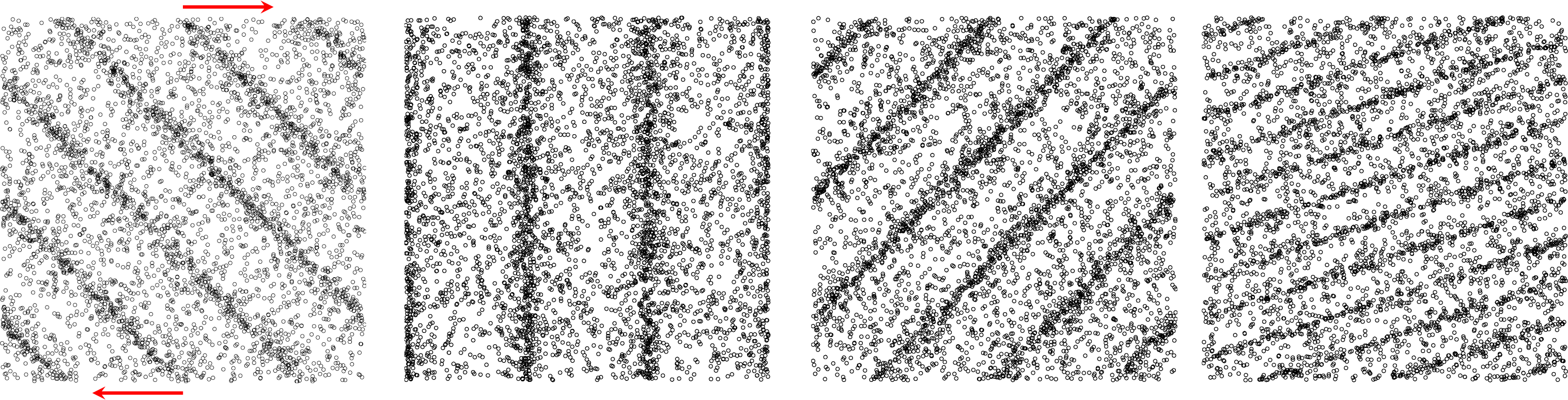
such that the final orientation is parallel to the shear gradient as illustrated in figure 2. Formally, this is described by
 $$\begin{eqnarray}\frac{\text{d}\boldsymbol{k}}{\text{d}t}=\unicode[STIX]{x1D735}(\unicode[STIX]{x1D6E4}y\boldsymbol{e}_{x})\boldsymbol{\cdot }\boldsymbol{k}\rightarrow k_{y}(t)=k_{y,0}-k_{x}\unicode[STIX]{x1D6E4}t.\end{eqnarray}$$
When the velocity gradient direction is parallel to gravity, the behaviour depicted in figure 1 and explained above might or might not be sampled depending on the initial orientation of the perturbations. Waves that are initially oriented upstream (
 $k_{x}k_{y}>0$
) sample the normal orientation (
 $k_{x}k_{y}=0$
) for a brief time before the shear further turn them downstream (
 $k_{x}k_{y}<0$
). The normal orientation is a configuration of maximum coupling between the two phases and strongest growth. Downstream waves do not sample this configuration and hence do not grow substantially. Once the wavevector is nearly parallel to both shear gradient and gravity, the result is nearly vertically stacked layers of higher and lower number density. The particle phase cannot drive fluid velocity perturbations anymore and growth ceases completely in the linear regime. The activation of nonlinear states will depend on the magnitude of the initial perturbation.
The homogeneous shear causes the turning of wave perturbations and the contraction of length scales. The sketch shows an initial upstream sinusoidal perturbation in the particle distribution strained at
 $\unicode[STIX]{x1D6E4}t=0,1,2$
and
 $4$
(left to right).
The growth and saturation of the number density has been studied with a linear stability analysis by Kasbaoui et al. (Reference Kasbaoui, Koch, Subramanian and Desjardins2015) for small heavy inertial solid particles in a gas. To make the derivation analytically tractable, an asymptotic solution to (2.12) was used in the LSA. Proposed by Ferry & Balachandar (Reference Ferry and Balachandar2001), the expansion is valid in the limit of small Stokes numbers
 $(St\ll 1)$
and leads to a relationship between the particle velocity and the local fluid velocity given by
 $$\begin{eqnarray}\boldsymbol{v}=\boldsymbol{u}+\boldsymbol{V}_{g}-\unicode[STIX]{x1D70F}_{p}\left(\frac{\unicode[STIX]{x2202}\boldsymbol{u}}{\unicode[STIX]{x2202}t}+(\boldsymbol{u}+\boldsymbol{V}_{g})\boldsymbol{\cdot }\unicode[STIX]{x1D735}\boldsymbol{u}+\unicode[STIX]{x1D6E4}y\frac{\unicode[STIX]{x2202}\boldsymbol{u}}{\unicode[STIX]{x2202}x}+\unicode[STIX]{x1D6E4}u_{y}\boldsymbol{e}_{x}\right)+O(\unicode[STIX]{x1D70F}_{p}^{2}).\end{eqnarray}$$
This expansion was introduced to make the analytical treatment of the linear stability analysis tractable. One needs only to solve the number density transport equation (2.11) with the evaluated particle velocity to completely describe the flow. However, there is no a priori way of determining how small the Stokes number needs to be for this expansion to be applicable.
In the LSA, the algebraic, non-modal growth of the instability was demonstrated with sinusoidal disturbances of the form
 $$\begin{eqnarray}\displaystyle & \displaystyle n(\boldsymbol{x},t)=\langle n\rangle +St\hat{n}(t)\exp (\text{i}(k_{x}x+k_{y}(t)y)), & \displaystyle\end{eqnarray}$$
 $$\begin{eqnarray}\displaystyle & \displaystyle \boldsymbol{u}(\boldsymbol{x},t)=\hat{\boldsymbol{u}}(t)\exp (\text{i}(k_{x}x+k_{y}(t)y)), & \displaystyle\end{eqnarray}$$
where the wavevector obeys (2.19),
 $\langle n\rangle =\langle \unicode[STIX]{x1D719}\rangle \unicode[STIX]{x03C0}d_{p}^{3}/6$
is the mean number density and
 $\hat{n}$
and
 $\hat{\boldsymbol{u}}$
are the wave amplitudes. The linearized evolution of the latter quantities is given by the coupled ordinary differential equations
 $$\begin{eqnarray}\frac{\text{d}\hat{n}}{\text{d}t}=-\text{i}\boldsymbol{V}_{g}\boldsymbol{\cdot }\boldsymbol{k}\hat{n}+\frac{\langle n\rangle }{\unicode[STIX]{x1D6E4}}\text{i}2\unicode[STIX]{x1D735}\boldsymbol{u}_{b}:\boldsymbol{k}\hat{\boldsymbol{u}},\end{eqnarray}$$
 $$\begin{eqnarray}\displaystyle \frac{\text{d}\hat{\boldsymbol{u}}}{\text{d}t} & = & \displaystyle -\!\left(\text{i}\frac{M}{1+M}\boldsymbol{V}_{g}\boldsymbol{\cdot }\boldsymbol{k}+\left(\boldsymbol{I}-2\frac{\boldsymbol{k}\boldsymbol{k}}{k^{2}}\right)\boldsymbol{\cdot }\unicode[STIX]{x1D735}\boldsymbol{u}_{b}^{\text{T}}+\frac{\unicode[STIX]{x1D708}}{1+M}k^{2}\right)\hat{\boldsymbol{u}}\nonumber\\ \displaystyle & & \displaystyle +\,\frac{\unicode[STIX]{x1D6E4}}{\langle n\rangle }\left(\boldsymbol{I}-\frac{\boldsymbol{k}\boldsymbol{k}}{k^{2}}\right)\frac{M}{1+M}\boldsymbol{V}_{g}\hat{n}.\end{eqnarray}$$
Although (2.24) is given in vectorial form, it is sufficient to solve for the velocity component along the gradient direction
 $y$
only. The other component can be found from the continuity equation
 $$\begin{eqnarray}k_{x}\hat{u} _{x}+k_{y}\hat{u} _{y}=0.\end{eqnarray}$$
Solutions to (2.23)–(2.25) constitute the LSA result (LSA) and will be compared to the full numerical solutions of the Euler–Lagrange (EL), two-fluid (TF) and anisotropic-Gaussian (AG) simulations.
3 Numerical strategies
3.1 Shear periodicity and homogeneous shear treatment
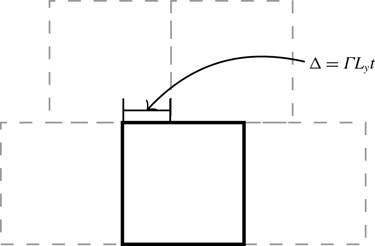
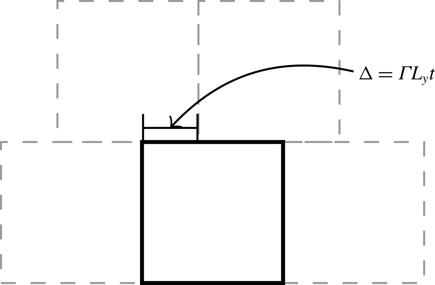
The numerical study of the present flow requires a specially crafted algorithm to capture the homogeneous shear effects. Our approach is described in Kasbaoui et al. (Reference Kasbaoui, Patel, Koch and Desjardins2017). Based on the earlier work of Baron (Reference Baron1982) and Gerz, Schumann & Elghobashi (Reference Gerz, Schumann and Elghobashi1989), the equations are solved in physical space without the need to remesh as in the popular method of Rogallo (Reference Rogallo1981). The key aspect is to enforce the so-called shear-periodic boundary conditions (see figure 3)
 $$\begin{eqnarray}f(x,Ly,z)=f(x-\unicode[STIX]{x1D6E4}tL_{y},0,z),\end{eqnarray}$$
where
 $f$
is any quantity of interest like the velocity fluctuation
 $\boldsymbol{u}$
, and
 $L_{y}$
is the extent of the computational domain in the shear gradient direction
 $y$
. The distortion terms
 $\unicode[STIX]{x1D6E4}y(\unicode[STIX]{x2202}f)/(\unicode[STIX]{x2202}x)$
are added directly in physical space in a split step approach. In the reference frame of the laboratory, these terms are responsible for the turning of the waves. Kasbaoui et al. (Reference Kasbaoui, Patel, Koch and Desjardins2017) show that this method is able to capture the rotation of the Fourier modes by the shear while maintaining their normal structure, an essential capability for the present study.
Shear-periodic boundary conditions.
3.2 Euler–Euler simulations
The appearance of clusters and void regions in the particle phase, call for special attention to the numerics used in Eulerian simulations. When clustering is significant, the volume fraction can drop significantly to near zero values in the neighbouring depleted regions. Positivity-preserving, also called realizable, Euler–Euler methods maintain positive volume fraction even when the solution is nearly devoid of particles (
 $\unicode[STIX]{x1D719}\rightarrow 0$
). Stability and mesh convergences of solvers for the dispersed phase are contingent on this property (Estivalezes & Villedieu Reference Estivalezes and Villedieu1996; Desjardins et al.
Reference Desjardins, Fox and Villedieu2008).
The particle-phase solver follows the quadrature based method of moments (Fox Reference Fox2008; Vi et al. Reference Vi, Doisneau and Massot2015; Kong et al. Reference Kong, Fox, Feng, Capecelatro, Patel, Desjardins and Fox2017). This is a realizable, second-order spatial discretization on a collocated mesh. The numerical strategy relies extensively on Lie operator splitting to ensure that every term in the governing equations is added in a realizable way. The distortion terms are treated in the same manner as in Kasbaoui et al. (Reference Kasbaoui, Patel, Koch and Desjardins2017).
At the beginning of the time step, we start by computing the drag term from the previous time step:
 $$\begin{eqnarray}\boldsymbol{D}^{n}=\frac{\unicode[STIX]{x1D719}^{n}\boldsymbol{u}^{n}-(\unicode[STIX]{x1D719}\boldsymbol{v})^{n}}{\unicode[STIX]{x1D70F}_{p}},\end{eqnarray}$$
where
 $(\unicode[STIX]{x1D719}\boldsymbol{v})^{n}$
is the particle momentum at the previous step treated as a whole. Note that the fluid solver mesh is staggered whereas the particle mesh is collocated, making interpolations of quantities from one mesh to the other necessary. At this point, we also compute the second-order drag tensor if using AG. Next, the pure convection of particle volume fraction, momentum and energy is advanced with a third-order Runge–Kutta scheme. For the volume fraction field this reads
 $$\begin{eqnarray}\displaystyle & \displaystyle \widetilde{\unicode[STIX]{x1D719}}=\unicode[STIX]{x1D719}^{n}-\text{d}t\unicode[STIX]{x1D735}\boldsymbol{\cdot }(\unicode[STIX]{x1D719}\boldsymbol{v})^{n}, & \displaystyle\end{eqnarray}$$
 $$\begin{eqnarray}\displaystyle & \displaystyle \widetilde{\widetilde{\unicode[STIX]{x1D719}}}={\textstyle \frac{3}{4}}\unicode[STIX]{x1D719}^{n}+{\textstyle \frac{1}{4}}(\widetilde{\unicode[STIX]{x1D719}}-\text{d}t\unicode[STIX]{x1D735}\boldsymbol{\cdot }\widetilde{(\unicode[STIX]{x1D719}\boldsymbol{v})}), & \displaystyle\end{eqnarray}$$
 $$\begin{eqnarray}\displaystyle & \displaystyle \overline{\unicode[STIX]{x1D719}}={\textstyle \frac{1}{3}}\unicode[STIX]{x1D719}^{n}+{\textstyle \frac{2}{3}}(\widetilde{\widetilde{\unicode[STIX]{x1D719}}}-\text{d}t\unicode[STIX]{x1D735}\boldsymbol{\cdot }\widetilde{\widetilde{(\unicode[STIX]{x1D719}\boldsymbol{v})}}), & \displaystyle\end{eqnarray}$$
where the numerical fluxes are computed with a second-order kinetic flux (Vikas et al. Reference Vikas, Wang, Passalacqua and Fox2011). Combined with a minmod slope limiter, the numerical fluxes are both stable in the presence of shocks and realizable for first-order forward in time integrations. The three stage Runge–Kutta extends this property to a realizable third-order time accurate integration by using convex combinations of realizable states. The overall scheme preserves the volume fraction positivity and is shock capturing.
Further updates are needed to add the remaining forces. In the next step, drag, gravity and convection of homogeneous shear by the fluctuations are added. For the particle momentum this reads
 $$\begin{eqnarray}\displaystyle \widehat{\unicode[STIX]{x1D719}\boldsymbol{v}}=\overline{\unicode[STIX]{x1D719}\boldsymbol{v}}-\text{d}t(\boldsymbol{D}^{n}+\boldsymbol{g}\unicode[STIX]{x1D719}^{n}-\unicode[STIX]{x1D6E4}(\unicode[STIX]{x1D719}v_{y})^{n}\boldsymbol{e}_{x}). & & \displaystyle\end{eqnarray}$$
This operation is also positivity preserving. The last remaining terms are the distortion terms
 $\unicode[STIX]{x1D6E4}y\unicode[STIX]{x2202}/(\unicode[STIX]{x2202}x)$
. These are added exactly using the characteristics method as in Kasbaoui et al. (Reference Kasbaoui, Patel, Koch and Desjardins2017)
 $$\begin{eqnarray}\displaystyle (\unicode[STIX]{x1D719}\boldsymbol{v})^{n+1}(\boldsymbol{x})=\widehat{\unicode[STIX]{x1D719}\boldsymbol{v}}(\boldsymbol{x}-\unicode[STIX]{x0394}t\unicode[STIX]{x1D6E4}y\boldsymbol{e}_{x}) & & \displaystyle\end{eqnarray}$$
and the boundary conditions are applied with time
 $n+1$
.
The algorithm then solves for the fluid phase using the method explained in Kasbaoui et al. (Reference Kasbaoui, Patel, Koch and Desjardins2017) and with the drag term
 $-\boldsymbol{D}^{n}$
interpolated to the fluid mesh as a source term.
3.3 Euler–Lagrange simulations
The Euler–Lagrange strategy follows the method of Capecelatro & Desjardins (Reference Capecelatro and Desjardins2013b
). The numerical method uses a volume-filtered approach that captures the particle modulation of the fluid without resolving the flow on the particle scale. The position and velocity of each Lagrangian particle (2.8) and (2.9) is advanced using a second-order Runge–Kutta scheme. Eulerian particle data such as the volume fraction field are computed from the Lagrangian data using a Gaussian kernel of width
 $\unicode[STIX]{x1D6FF}_{f}$
multiple of the particle diameter. The unperturbed fluid velocity at the particle location is computed using the method of Ireland & Desjardins (Reference Ireland and Desjardins2017). This quantity is required for the correct calculation of the drag force and leads to correct predictions of the particle settling velocity. The method is fully conservative and yields grid-independent solutions in two-way coupled problems and has been verified against experiments (Capecelatro & Desjardins Reference Capecelatro and Desjardins2013a
; Capecelatro, Pepiot & Desjardins Reference Capecelatro, Pepiot and Desjardins2014).
The imposed homogeneous shear necessitates some additions. The shear term in (2.8) generally poses no computational challenges. Particles leaving from the top and bottom of the domain (
 $y=\pm L_{y}/2$
) are reintroduced from the other side with translated
 $x$
position and velocity. This procedure is the well-known Lees–Edwards boundary conditions (Lees & Edwards Reference Lees and Edwards1972) and is the discrete analogue of the shear-periodic boundary conditions (3.1).
4 Linear regime: the preferential concentration instability
In this section, we simulate a homogeneously sheared particle-laden flow traversed by a small velocity perturbation. We seek to demonstrate the shear instability in a practical case that allows comparison with the linear stability analysis. The simulations are conducted with the EL, TF and AG methodologies. Comparisons with the LSA serve to validate the numerical strategies. Comparisons among the three methodologies are intended to assess the importance of the discrete nature of the particulate phase and the occurrence of particle-trajectory crossing.
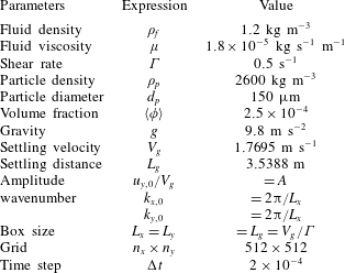
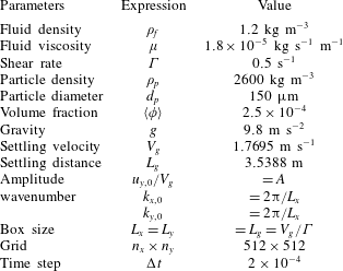
The flow parameters are shown in table 1. Glass beads of diameter
 $d_{p}=150~\unicode[STIX]{x03BC}\text{m}$
and density
 $\unicode[STIX]{x1D70C}_{p}=2600~\text{kg}~\text{m}^{-3}$
are suspended in air at standard temperature and pressure. The shear rate is
 $\unicode[STIX]{x1D6E4}=0.5~\text{s}^{-1}$
and gravity is
 $g=9.8~\text{m}~\text{s}^{-2}$
. The Stokes number here,
 $St=0.09$
, falls in the range of small stokes numbers for which the expansion (2.20) is believed to be applicable. The Reynolds number is
 $Re=\unicode[STIX]{x1D70C}_{f}V_{g}L_{g}/\unicode[STIX]{x1D707}_{f}=1.05\times 10^{5}$
. Although the average volume fraction is small,
 $\langle \unicode[STIX]{x1D719}\rangle =2.5\times 10^{-4}$
, the mass loading
 $M=0.54$
is
 $O(1)$
owing to the large ratio
 $\unicode[STIX]{x1D70C}_{p}/\unicode[STIX]{x1D70C}_{f}$
of the density of glass beads to that of the gas. These parameters allow strong two-way coupling between the two phases via gravity and preferential concentration.
The choice of computational box size and resolution is guided by the analysis of the different wavelength perturbations in the LSA. According to the linear analysis, large-scale perturbations have a typical wavelength comparable to the particle settling distance in one shear time
 $L_{g}=V_{g}/\unicode[STIX]{x1D6E4}$
. On the other end, small-scale perturbations of the size of the dissipation scale
 $L_{\unicode[STIX]{x1D707}}=\sqrt{\unicode[STIX]{x1D707}/(\unicode[STIX]{x1D70C}_{f}\unicode[STIX]{x1D6E4})}$
are rapidly suppressed. To resolve all scales, we set the two-dimensional computational domain dimensions to
 $L_{x}=L_{y}=L_{g}$
and use 512 grid points in each direction to ensure an adequate resolution of the dissipative scales (
 $\unicode[STIX]{x0394}x/L_{\unicode[STIX]{x1D707}}\sim 1.2$
). The Lagrangian particle filter has a width
 $\unicode[STIX]{x1D6FF}_{f}=47d_{p}$
, approximately equal to the grid spacing
 $\unicode[STIX]{x0394}x$
.
Simulation parameters for the standard case of
 $St=0.09$
and
 $M=0.5$
.
A large-scale sinusoidal perturbation with
 $k_{x}=2\unicode[STIX]{x03C0}/L_{g}$
initiated in the oblique direction
 $x=y$
at
 $t=0$
drives the particle and fluid initial velocities. The initial fluid velocity field is given by (2.22), which is then used to generate the particle velocity field according to the expression (2.20). The initial orientation,
 $k_{y,0}/k_{x}=1$
, allows the perturbation to sample the direction of strongest particle–fluid coupling (
 $k_{y}=0$
) during the turning of the wave and experience considerable growth. In Euler–Euler simulations, the initial volume fraction field is uniform. The particle velocity field is initialized by direct evaluation of expression (2.20). In Euler–Lagrange simulations, expression (2.20) is evaluated at the particle location to determine the Lagrangian particle velocities. Moreover, the particles are seeded randomly in the domain. At the average volume fraction
 $\langle \unicode[STIX]{x1D719}\rangle =2.5\times 10^{-4}$
and for particles in table 1, the two-dimensional simulation domain contains approximately
 $2.8\times 10^{6}$
particles.
When the perturbation strength
 $A$
, the ratio of the perturbation magnitude to the settling velocity, is sufficiently small, a linear evolution of the mode is expected. The linear stability analysis does not provide an indication on how small
 $A$
needs to be to remain in the linear regime. However, one can expect nonlinearities to manifest if the amplified perturbation was to reach a magnitude comparable to the base state. For the driving initial mode,
 $k_{x}^{\star }=L_{g}k_{x}/(2\unicode[STIX]{x03C0})=1$
, the LSA predicts a total amplification
 $\unicode[STIX]{x1D719}_{rms}(k_{x}^{\star }=1)/(A\langle \unicode[STIX]{x1D719}\rangle )\simeq 7$
, where
 $\unicode[STIX]{x1D719}_{rms}$
is the volume fraction fluctuation root mean square (r.m.s.). Consequently, for
 $A\ll 0.14$
one can expect a linear evolution owing to the small total amplification,
 $\unicode[STIX]{x1D719}_{rms}\ll \langle \unicode[STIX]{x1D719}\rangle$
, whereas, cases such that
 $A>0.14$
can be expected to evolve nonlinearly.
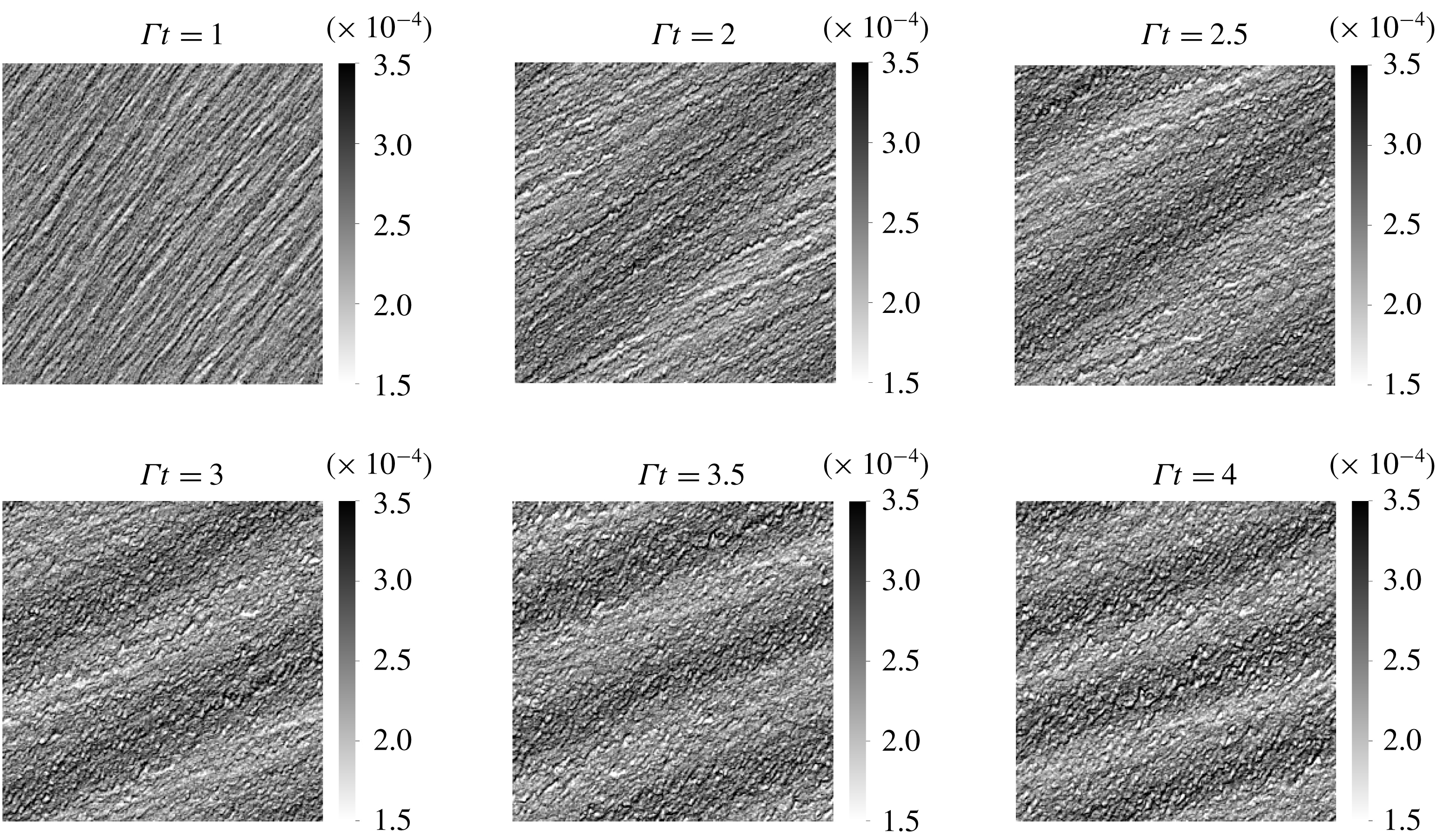
Snapshots of the volume fraction field in EL simulation with perturbation strength
 $A=0.02$
.
Snapshots of the volume fraction field in TF simulation with perturbation strength
 $A=0.02$
.
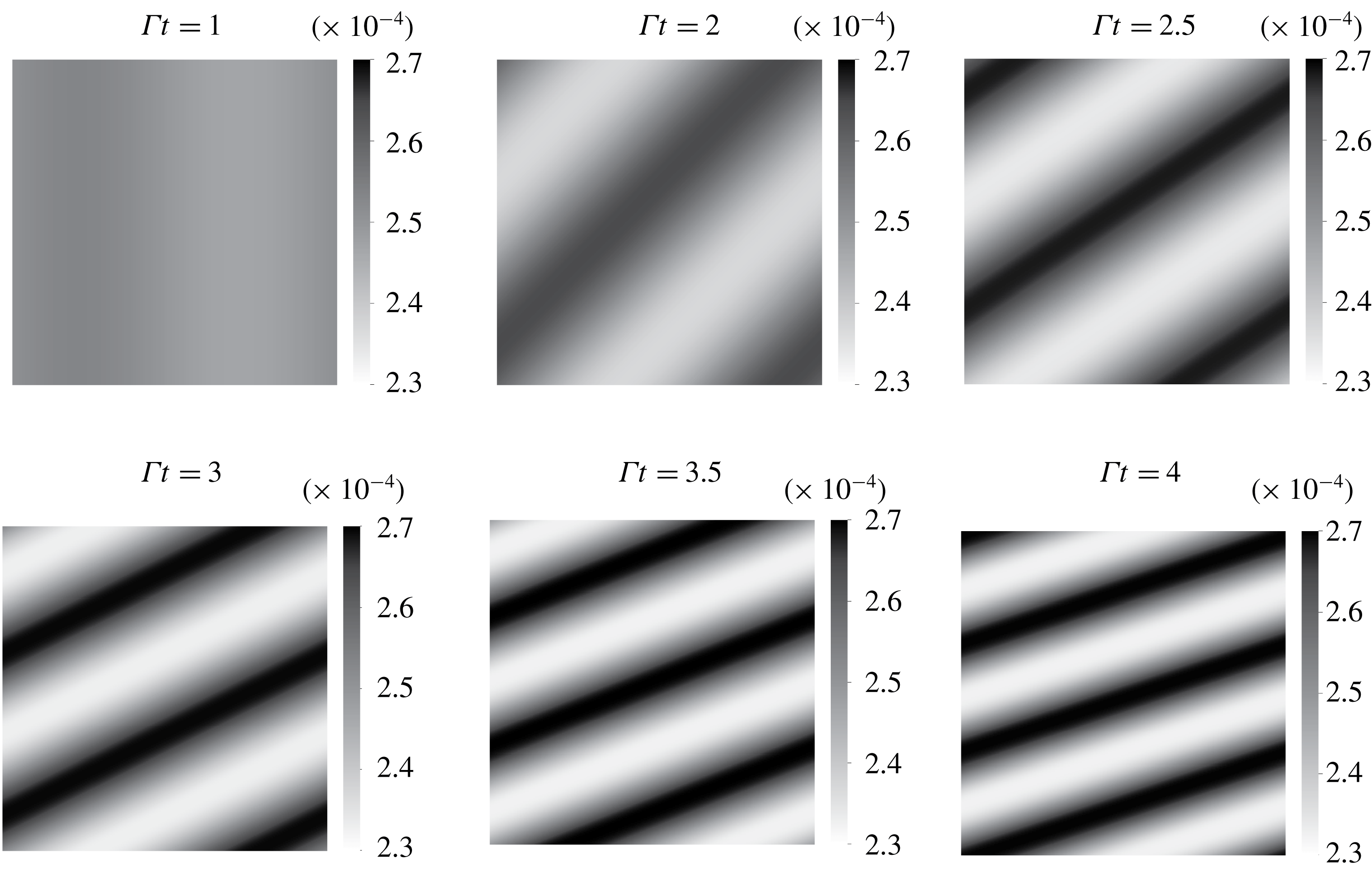
The case in table 1 is simulated with EL and TF methods for the initial perturbation strength
 $A=0.02$
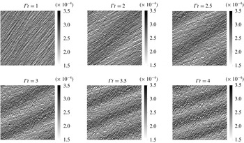
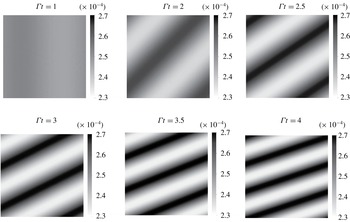
. Snapshots of EL and TF simulations (see figures 4 and 5 respectively) show the emergence of a sinusoidal perturbation in the volume fraction field. The turning of the perturbation is induced by the background base shear as explained in § 2.2 and depicted by the sketch in figure 2. The wavelength can be seen contracting owing to a compression of scales in the gradient direction.
The EL simulations show the existence of small-scale perturbations in addition to the driving large-scale mode. These perturbations are induced by the random distribution of the Lagrangian particles. They appear as streaky features in the volume fraction field at
 $\unicode[STIX]{x1D6E4}t=1$
which then destabilize and form small bubbles depleted of particles. The streaky features could be interpreted as the preferential concentration instability happening at small scales. In fact, according to the LSA, the fastest growing modes are approximately ten times larger than the dissipation scale
 $L_{\unicode[STIX]{x1D707}}$
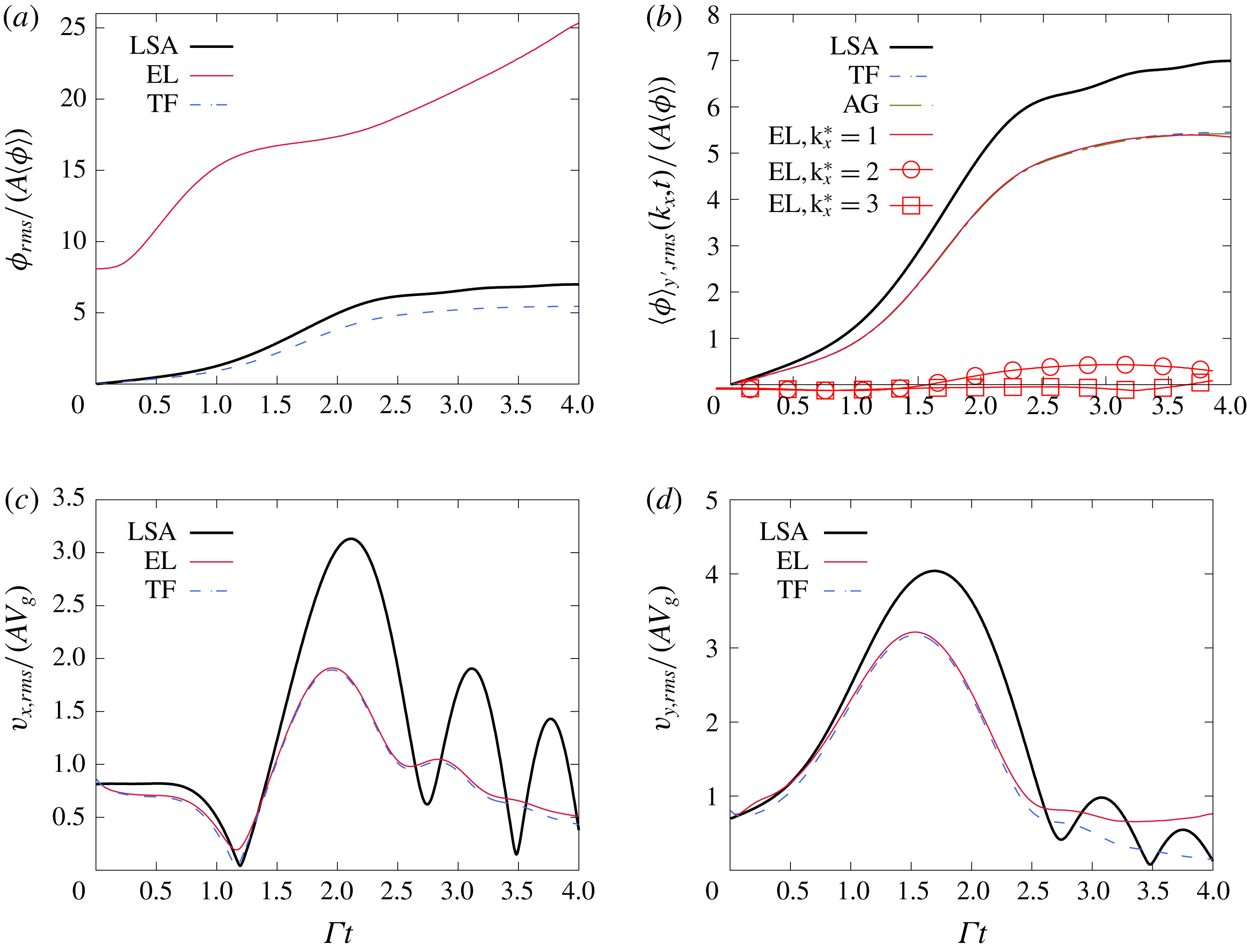
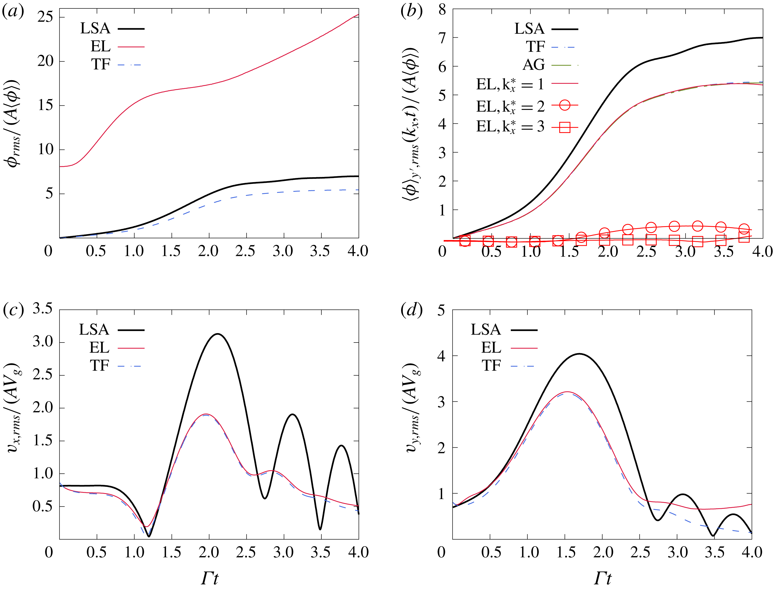
which explains the short wavelength of these streaky perturbations. Because the TF data do not contain these short wavelength perturbations, direct comparisons with the EL data is difficult. Figure 6(a) shows the evolution of the r.m.s. volume fraction fluctuations,
 $\unicode[STIX]{x1D719}_{rms}$
, in EL and TF simulations. At
 $t=0$
,
 $\unicode[STIX]{x1D719}_{rms}$
is already non-zero in EL simulations due to the random distribution of particles. The quantity
 $\unicode[STIX]{x1D719}_{rms}$
encompasses the effects of modes at all scales resulting in the large deviation between the TF and EL evolutions seen in figure 6(a).
Time evolution of the fluctuations traversing the flow. (a) Shows the r.m.s. volume fraction fluctuations. The large deviation of the EL curve compared to the LSA and TF simulations is a consequence of the fluctuations introduced by the random distribution of the Lagrangian particles. Extracting the fluctuations associated with the mode
 $k_{x}^{\star }=k_{x}L_{g}/(2\unicode[STIX]{x03C0})=1$
in EL (b) shows a nearly identical evolution of to the TF and AG simulations. Fluctuations associated with the modes
 $k_{x}^{\star }=2$
and 3 in EL simulations are also shown to remain small in this linear regime. The r.m.s. fluctuations of the horizontal (c) and vertical (d) particle velocities evolve similarly in EL and TF simulations and reproduce the same oscillatory behaviour seen from the LSA. The flow parameters are as in table 1 and correspond to
 $\langle \unicode[STIX]{x1D719}\rangle =2.5\times 10^{-4}$
,
 $M=0.54$
and
 $St=0.09$
. The perturbation strength is
 $A=0.02$
.
For a meaningful comparison with the TF volume fraction, it is essential to separate the effects of the imposed perturbation from other fluctuations present in EL simulations. The procedure adopted here is to compute the Fourier spectrum of the volume fraction field
 $\unicode[STIX]{x1D719}$
in the sheared reference frame
 $x^{\prime }=x-\unicode[STIX]{x1D6E4}ty$
and
 $y^{\prime }=y$
and extract the imposed mode
 $k_{x}^{\star }=1$
. The complex amplitude associated with the Fourier mode
 $k_{x}$
reads as
 $$\begin{eqnarray}\displaystyle \langle \hat{\unicode[STIX]{x1D719}}(k_{x},t)\rangle _{y^{\prime }}=\frac{1}{L_{y}}\int _{y^{\prime }}\left(\int _{x^{\prime }}\unicode[STIX]{x1D719}(x^{\prime }+\unicode[STIX]{x1D6E4}ty^{\prime },y^{\prime })\text{e}^{\text{i}2\unicode[STIX]{x03C0}k_{x}x^{\prime }}\,\text{d}x^{\prime }\right)\,\text{d}y^{\prime }, & & \displaystyle\end{eqnarray}$$
where
 $\langle \cdot \rangle _{y^{\prime }}$
denotes the average over the direction
 $y^{\prime }=y$
. The larger sample pool yields better converging statistics. It is also important to realize that this averaging removes fluctuations in the transverse direction to the wave. Computing ‘frozen’ Fourier modes in the sheared reference frame is equivalent to computing the rotating Fourier modes explained in § 2.2. Spectral interpolations are used to evaluate off grid points in
 $\unicode[STIX]{x1D719}(x^{\prime }+\unicode[STIX]{x1D6E4}ty,y)$
. The r.m.s. fluctuation associated with the mode
 $k_{x}$
is
 $$\begin{eqnarray}\displaystyle \langle \unicode[STIX]{x1D719}\rangle _{y^{\prime },rms}(k_{x},t) & = & \displaystyle \sqrt{\langle (\langle \hat{\unicode[STIX]{x1D719}}(k_{x},t)\rangle _{y^{\prime }}\text{e}^{\text{i}2\unicode[STIX]{x03C0}k_{x}x^{\prime }}+\langle \hat{\unicode[STIX]{x1D719}}(-k_{x},t)\rangle _{y^{\prime }}\text{e}^{-\text{i}2\unicode[STIX]{x03C0}k_{x}x^{\prime }})^{2}\rangle _{x^{\prime }}}\nonumber\\ \displaystyle & = & \displaystyle \sqrt{2(\text{Re}\{\langle \hat{\unicode[STIX]{x1D719}}(k_{x},t)\rangle _{y^{\prime }}\}^{2}+\text{Im}\langle \{\hat{\unicode[STIX]{x1D719}}(k_{x},t)\}^{2}\rangle _{y^{\prime }})}.\end{eqnarray}$$
Figure 6(b) shows the first three extracted modes from EL simulations. The extracted mode
 $k_{x}^{\star }=1$
follows closely the EE simulations for much of the integration time. Small departure beyond
 $\unicode[STIX]{x1D6E4}t\sim 3.5$
occurs concomitantly with the growth of the second mode and third modes
 $k_{x}=2$
and
 $3$
. The initial random distribution of the particles helps seed modes. Although they start with significantly smaller amplitudes than
 $k_{x}$
, these modes can grow comparatively faster. In this small perturbation case, their total amplification remains small for
 $\unicode[STIX]{x1D6E4}t\leqslant 4$
.
The particle velocity fluctuations r.m.s. are shown in figure 6(c,d). The TF and EL simulations match well in this linear case. The simulations show a similar oscillatory behaviour as the one predicted by the LSA. Notice that compressibility effects can be seen in the plot of
 $v_{x}$
, since a solenoidal particle velocity field would imply the relation
 $v_{x}\sim -k_{y}/k_{x}v_{y}$
leading to
 $v_{x}=0$
at the time
 $k_{y}$
cancels, i.e.
 $\unicode[STIX]{x1D6E4}t=1$
. It is seen in figure 6(d) that vertical fluctuations
 $v_{rms}$
persist even at long times. These fluctuations are in the downward direction, and lead to higher particle settling rates. In the literature of particle-laden turbulence, this is referred to as preferential sweeping (Wang & Maxey Reference Wang and Maxey1993; Yang & Lei Reference Yang and Lei1998; Aliseda et al.
Reference Aliseda, Cartellier, Hainaux and Lasheras2002; Yang & Shy Reference Yang and Shy2005; Good et al.
Reference Good, Ireland, Bewley, Bodenschatz, Collins and Warhaft2014; Ireland, Bragg & Collins Reference Ireland, Bragg and Collins2016). The deviation of the EL curve from the TF one near
 $\unicode[STIX]{x1D6E4}t\sim 3.5$
proves that the long-time persistent particle sweeping is enhanced by the small-scale perturbations in EL simulations.
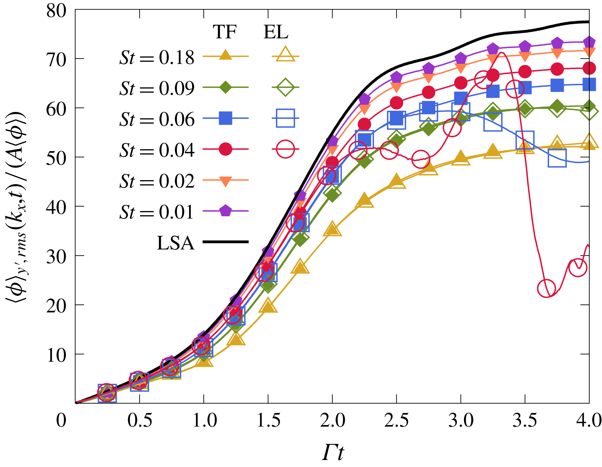
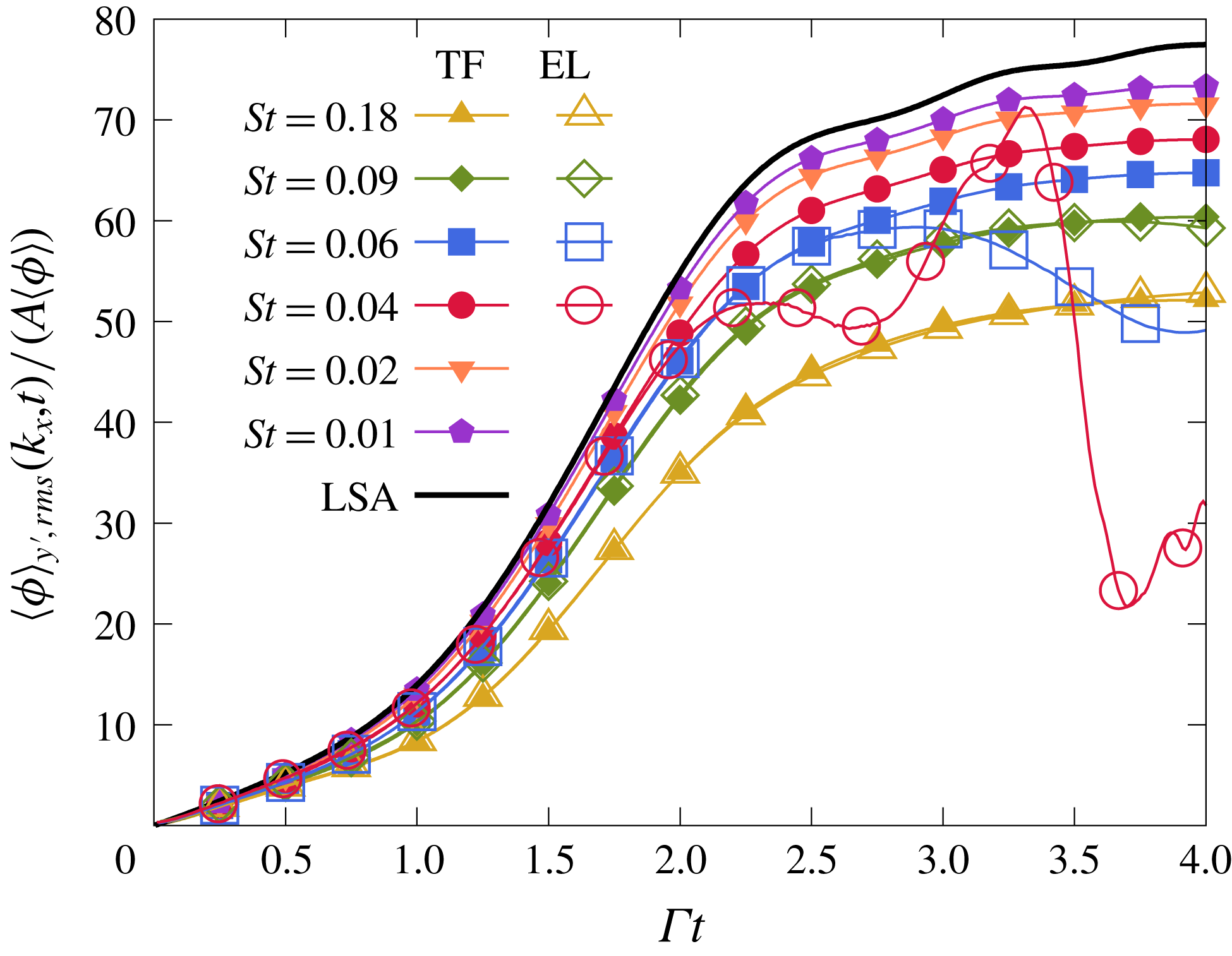
In both EL and TF simulations, the volume fraction and particle velocity fluctuations display similar time dependence to the LSA predictions, but a departure remains at long times. These differences are controlled by the Stokes number. Figure 7 shows how diminishing
 $St$
leads to the convergence of TF and EL volume fraction to the LSA results. The lowering of
 $St$
from
 $St=0.18$
to
 $St=0.01$
moves the TF curves upwards towards the LSA curve, which remains an upper limit. As explained in § 2, the small Stokes expansion (2.20) implies that the LSA is valid in the double limit of small perturbations (
 $A\ll 1$
) and very small particle inertia (
 $St\ll 1$
). Despite the significantly better agreement at
 $St=0.01$
, the volume fraction fluctuations remain higher for the larger Stokes numbers because the total amplification is proportional to the product
 $StA$
. For the same reasons as in TF simulations, the lowering of
 $St$
number from
 $0.18$
to
 $0.04$
moves the EL curves upwards towards the LSA one. However, the diminishing signal (proportional to
 $St$
) results in the small-scale perturbations, initiated by the random distribution of particles, gaining in relative strength. The destruction of the seeded large scale mode
 $k_{x}^{\star }=1$
, shows the difficulty of establishing comparisons with EL methods for very small Stokes number particles. Note that the variation of the Stokes number
 $St=\unicode[STIX]{x1D6E4}\unicode[STIX]{x1D70F}_{p}$
was achieved by varying the shear rate, rather than the particle density
 $\unicode[STIX]{x1D70C}_{p}$
to keep the mass loading constant. One could also vary the particle diameter in order to change the Stokes number, however, at the same average volume fraction, smaller particles lead to a higher total count requiring more computational resources. We also vary the gravitational acceleration proportionally in order to maintain an identical box size
 $L_{x}=L_{g}=g\unicode[STIX]{x1D70F}_{p}/\unicode[STIX]{x1D6E4}$
. This ensures an equal count of particles per cell across all EL simulations and provides sufficient sampling for the computation of particle quantities.
Effect of varying the Stokes number in EL and TF simulations.
Lastly, we address the results of AG in the linear regime. Figure 6(b) shows little difference with the TF method for the case with
 $A=0.02$
and
 $St=0.09$
. As mentioned before, an anisotropic-Gaussian number density pdf collapses onto a mono-kinetic pdf for very small
 $St$
number yielding the TF governing equations. The near identical TF and AG evolutions in figure 6(b) show that particle-trajectory effects modelled by the AG distribution are absent in the linear regime. By reciprocity, AG also agrees with the EL simulations. Based on the quantitatively similar growth of the mode
 $k_{x}^{\star }=1$
observed with all three simulation strategies, we conclude that particle-trajectory crossing is negligible for small inhomogeneities traversing a semi-dilute flow with small Stokes number particles. However, as we show in the next section, when nonlinearities develop, severe out-of-equilibrium states take place leading to distinctly different evolutions for the three methods.
5 Nonlinear regime: secondary Rayleigh–Taylor instability and caustics
Understanding the mechanisms leading to clustering in turbulent flows is often rendered difficult by the presence of multiple of length scales. Instead, we focus on clustering in the presence of a single perturbed velocity mode. Looking at the nonlinear regime in this flow configuration, we propose to establish a route to clustering that unveils the principal mechanisms at play in two-way coupled semi-dilute flows. As we show below, these mechanisms are: the preferential concentration instability, particle-trajectory crossing, and the Rayleigh–Taylor instability.
5.1 Nonlinearities in EL formulation
We start with the analysis of the nonlinearities in EL simulations. The case in table 1 is run with an initial perturbation strength
 $A=0.25$
. At this level, a strong deviation from the linear evolution is guaranteed, since according to the LSA, the sinusoidal volume fraction perturbation would grow so much that the depleted regions, the troughs of the sinusoid, would have a non-physical negative volume fraction. Hence, it is expected that large void regions form and that the sinusoid deforms nonlinearly.
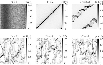
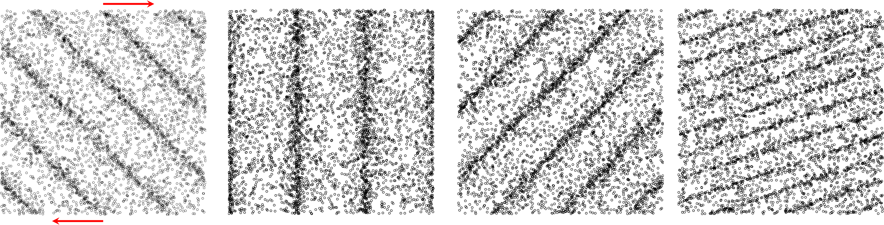
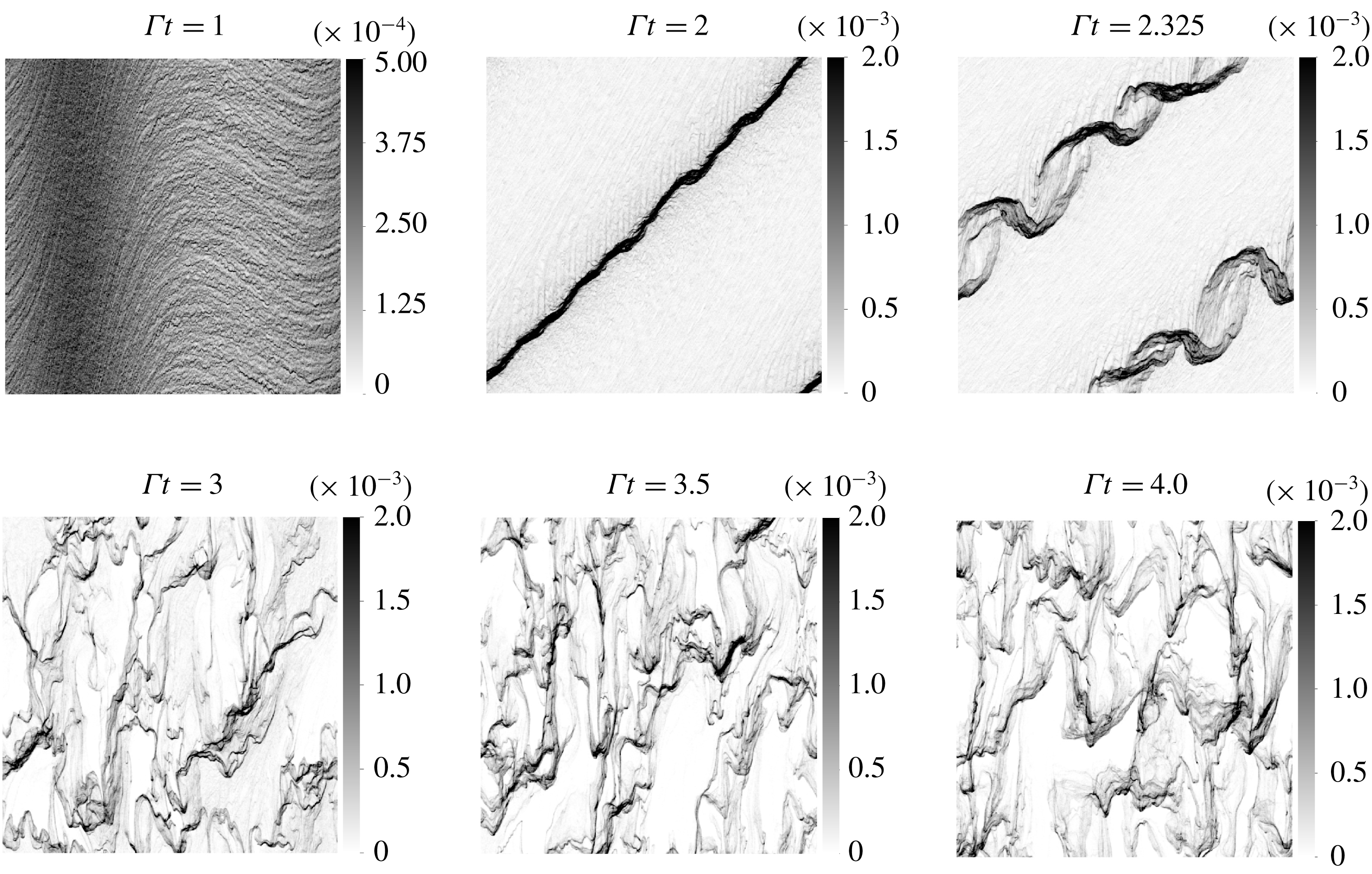
Snapshots of the volume fraction field in EL simulation for the large perturbation strength
 $A=0.25$
. A secondary transverse Rayleigh–Taylor instability breaks the sheet of particles formed by the primary preferential concentration. The final state displays sustained clustering.
Snapshots of the volume fraction field during
 $1\leqslant \unicode[STIX]{x1D6E4}t\leqslant 4$
(see figure 8) show the gradual evolution towards a state dominated by clusters similar to those seen in the grid turbulence experiments of Yang & Shy (Reference Yang and Shy2005) with copper beads (
 $\langle \unicode[STIX]{x1D719}\rangle =5\times 10^{-5}$
,
 $M=0.5$
,
 $St=0.36$
). First, the preferential concentration instability causes the extreme accumulation of particles along the oblique direction of the rotating perturbation during
 $0<\unicode[STIX]{x1D6E4}t<2$
. Nearly all of the particles are distributed on a sheet of small thickness. Despite the stronger nonlinear amplification, this first stage is qualitatively understood from the LSA and the simulations in the linear regime. Shortly after, a transverse instability manifests around
 $\unicode[STIX]{x1D6E4}t=2.1$
and is clearly visible on the snapshot at
 $\unicode[STIX]{x1D6E4}t=2.325$
. This secondary instability is of a Rayleigh–Taylor type as we explain below. It adds spatial dimensionality to the particle distribution by breaking the quasi-one-dimensional long band of particles formed by the preferential concentration instability. Notice that this secondary instability grows in a double helix shape: two modes in antiphase grow simultaneously. These modes grow on a time scale much smaller than the shear time
 $\unicode[STIX]{x1D6E4}^{-1}$
and lead to the formation of clusters seen in the snapshots at
 $\unicode[STIX]{x1D6E4}t=3$
, 3.5 and 4.
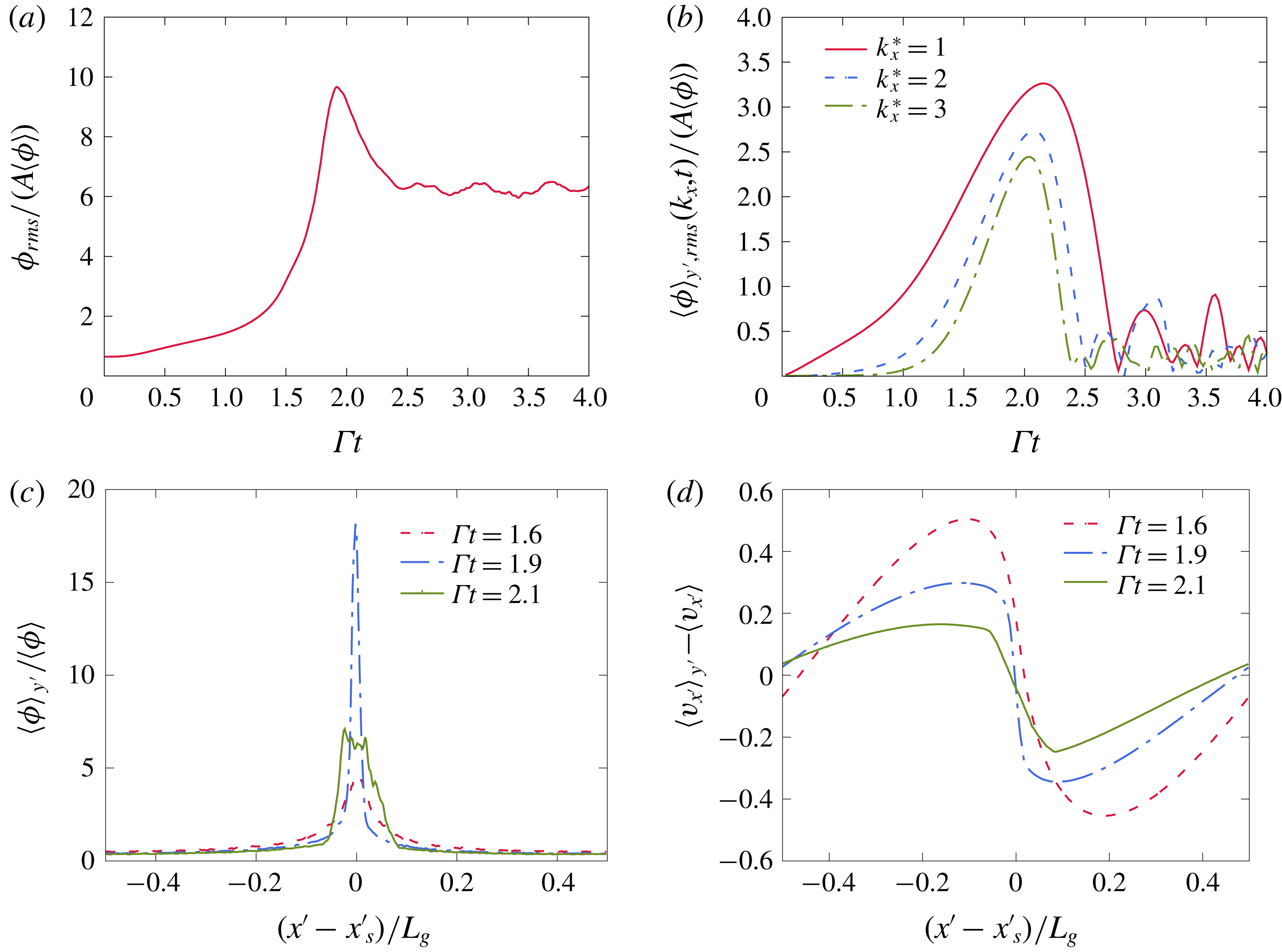
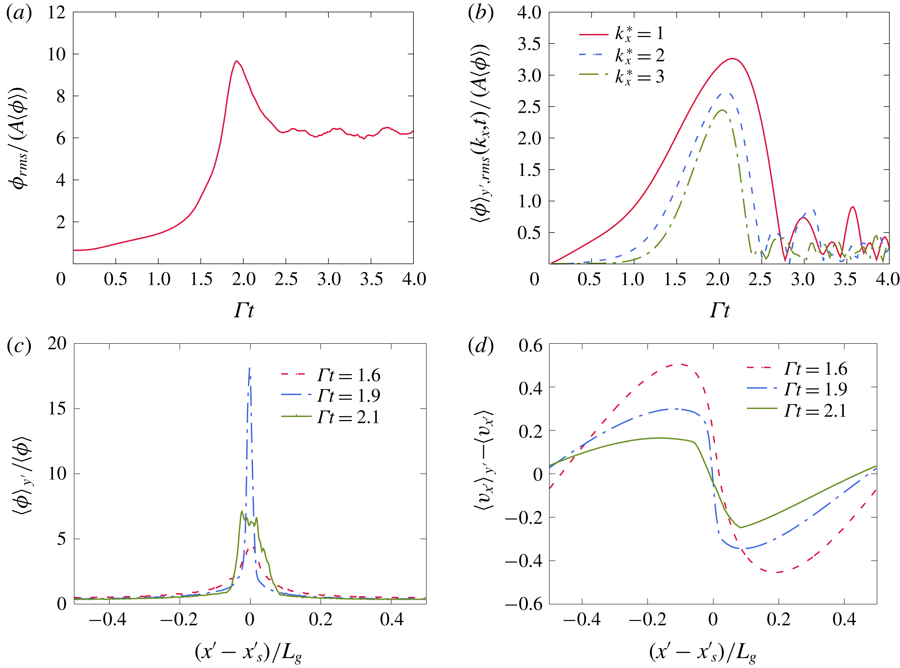
Evolution of the perturbation in the EL simulation. (a) Shows the fluctuations peak around
 $\unicode[STIX]{x1D6E4}t\sim 2$
. (b) Shows significant growth of the unperturbed modes
 $k_{x}^{\star }=2$
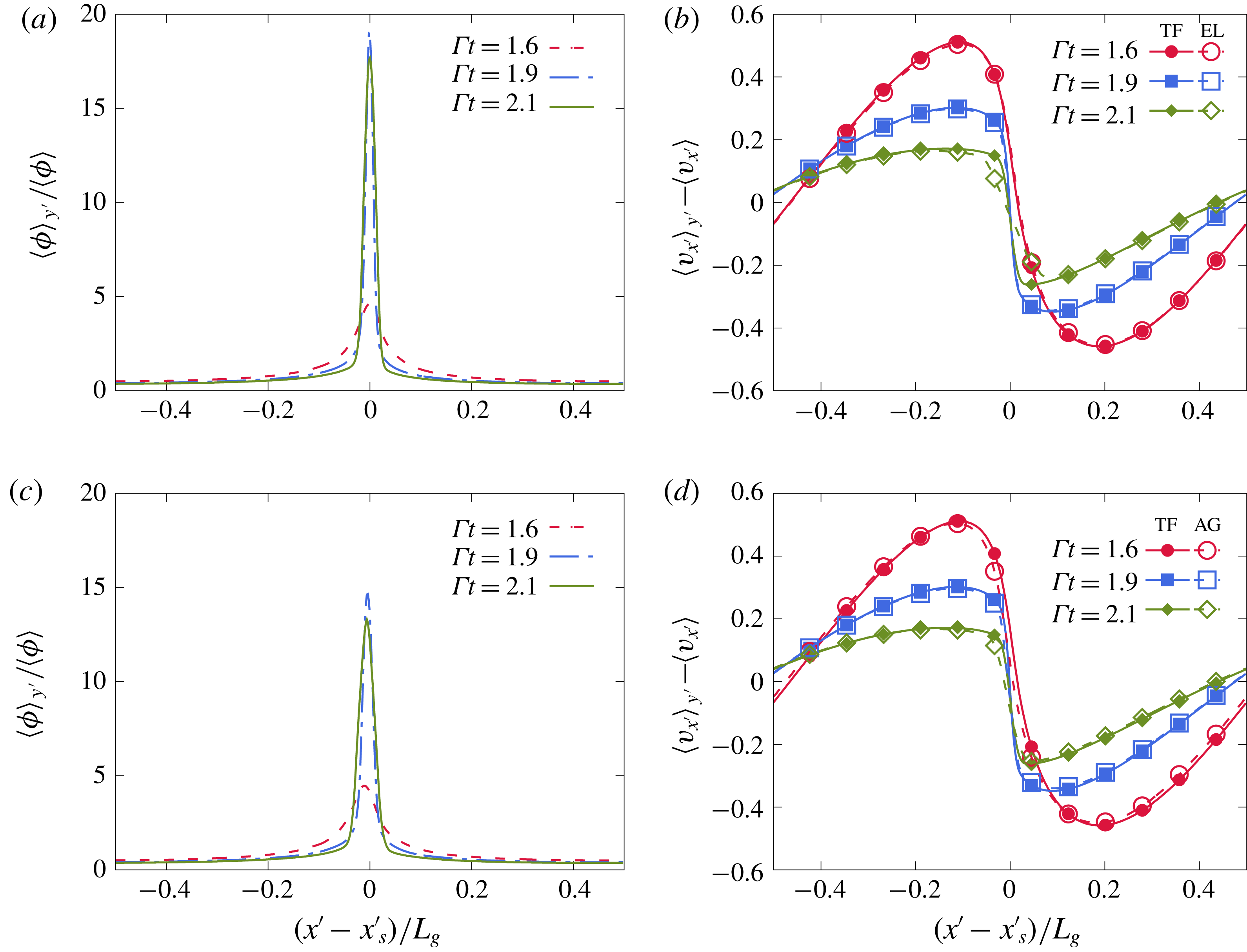
and 3. The collapse of these modes coincides with the appearance of the transverse secondary instability. (c,d) Show the volume fraction and wave-normal particle velocity as a function of the wave-normal coordinate
 $x^{\prime }=\boldsymbol{k}\boldsymbol{\cdot }\boldsymbol{x}/k$
centred on the high concentration band of particles. The steepening of the sinusoidal wave leads to a volume fraction shaped like an impulse (
 $\unicode[STIX]{x1D6E4}t=1.6$
and 1.9). Particle-trajectory crossing leads to the spreading of the profiles at
 $\unicode[STIX]{x1D6E4}t=2.1$
.
5.1.1 Preferential concentration instability
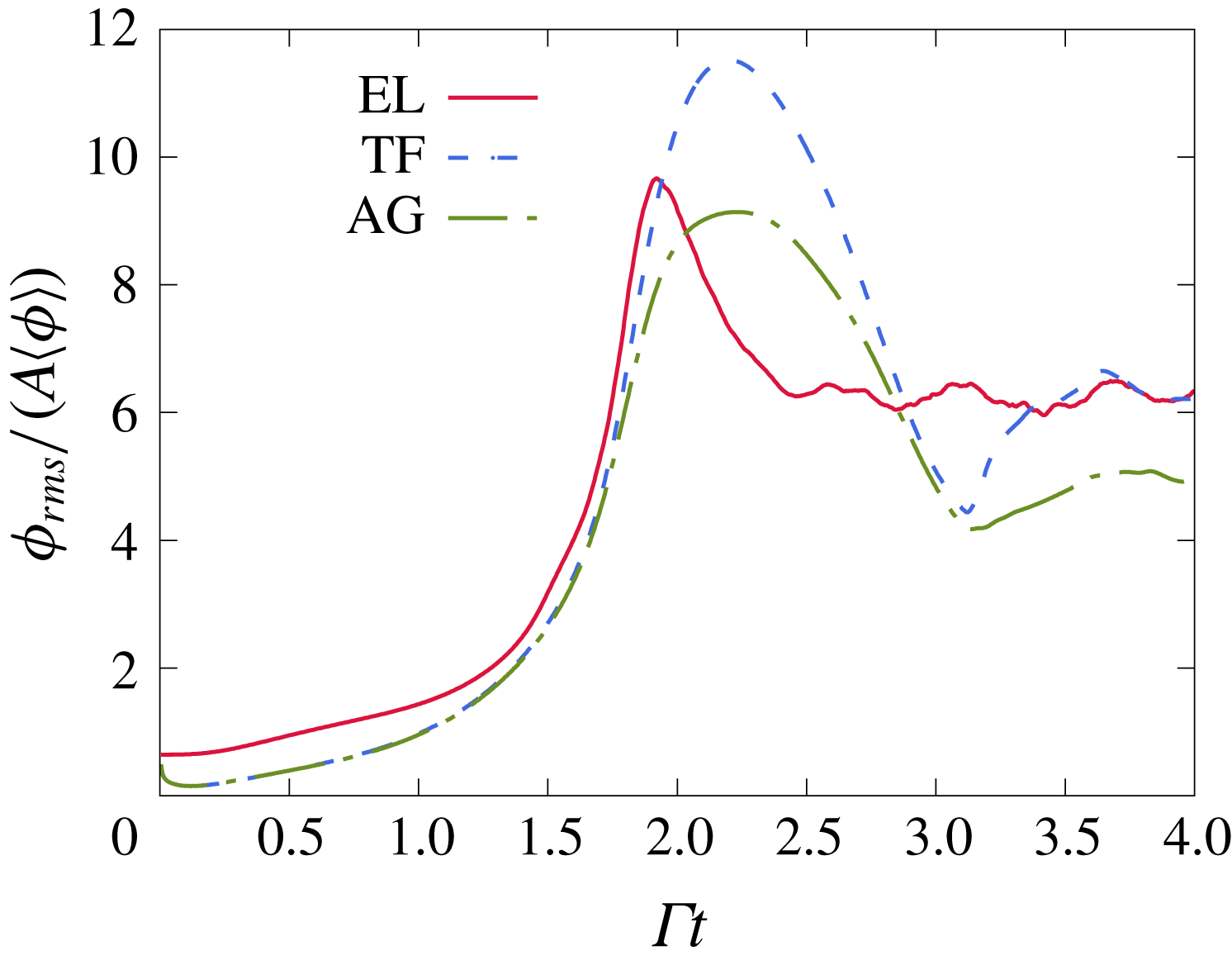
Figure 9(a) shows the time evolution of the volume fraction fluctuation. One can see a clearly different evolution from the linear case in figure 6(a). The volume fraction fluctuations grow linearly until
 $\unicode[STIX]{x1D6E4}t\sim 1.5$
, after which a sharp peak is attained around
 $\unicode[STIX]{x1D6E4}t=2$
. The total volume fraction fluctuation then drops and eventually plateaus by the end of the simulation. Figure 9(b) shows that, in addition to the initialized mode
 $k_{x}^{\star }=1$
, the shorter wavelength modes
 $k_{x}^{\star }=2$
and 3 are also strongly amplified. These modes exist initially because the random distribution of particles creates perturbations at all scales. In the nonlinear regime, these modes grow nearly as large as the one seeded by the deterministic perturbation. These modes collapse when the transverse perturbations appear, around
 $\unicode[STIX]{x1D6E4}t\sim 2.1$
. Figure 9(c) shows the normalized volume fraction averaged over the transverse direction and plotted as a function of the wave-normal coordinate
 $x^{\prime }=(\boldsymbol{k}\boldsymbol{\cdot }\boldsymbol{x})/k$
. The plots at the consecutive times
 $\unicode[STIX]{x1D6E4}t=1.6$
, 1.9 show the gradual concentration of the field into an impulse function reaching a peak nearly 18 times higher than the average volume fraction. Such high particle concentrations have also been observed in particle-laden turbulent simulations. Squires & Eaton (Reference Squires and Eaton1991) report a volume fraction inside clusters reaching 25 times the average volume fraction in EL simulations of homogeneous isotropic turbulence with
 $St=0.15$
particles.
5.1.2 Caustics and particle-trajectory crossing
The two antiphase transverse modes forming the double helix (snapshot at
 $\unicode[STIX]{x1D6E4}t=2.325$
in figure 8) originate from two streams of particles that cross at the high concentration sheet. To understand how this takes place, we report the Eulerian wave-normal particle velocity
 $v_{x^{\prime }}=(\boldsymbol{k}\boldsymbol{\cdot }\boldsymbol{v})/k$
, where
 $\boldsymbol{v}$
is the Eulerian particle velocity computed from the Lagrangian data on the mesh. The figure shows clear steepening of the original sinusoidal wave. This nonlinear process occurs as particles migrate to the location of the high concentration sheet. Particles from the two sides move in two opposing streams causing the slope of the centred wave-normal velocity to steepen and the volume fraction impulse to sharpen. When the two streams meet, around
 $\unicode[STIX]{x1D6E4}t=2.1$
, particle-trajectory crossing takes place, i.e. the two streams inter-penetrate and continue moving in opposite directions. This has four consequences. First, the gradient of the wave-normal velocity
 $v_{x^{\prime }}$
drops, as seen in figure 9(d), due to the presence of particles with opposing velocities within one grid cell in the crossing zone. Second, the crossing of the streams leads to the spreading of the volume fraction impulse (see figure 9
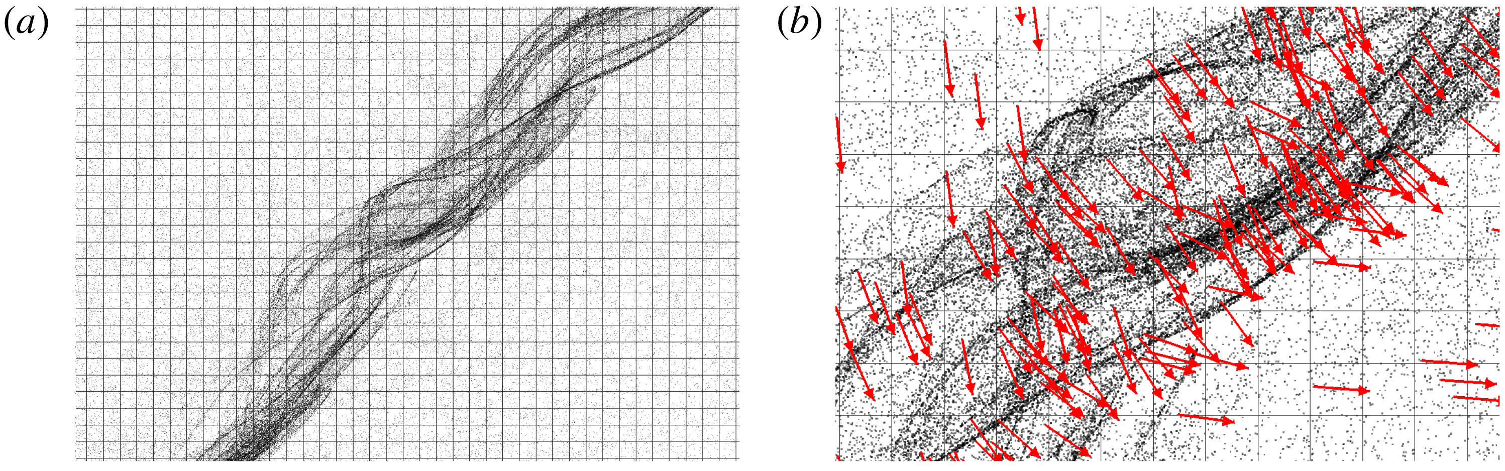
c). Third, particle-trajectory crossing is known to manifest as caustics (Gustavsson et al.
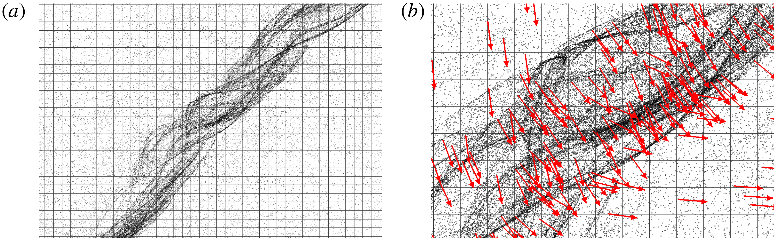
Reference Gustavsson, Meneguz, Reeks and Mehlig2012), long intersecting filaments of aligned particles. This can be seen in figure 10(a) in a zoomed-in view around the high concentration sheet. Fourth, the crossing of the particle streams along with transverse perturbations lead to particles within one grid cell having non-parallel velocity vectors (see figure 10
b).
Snapshots of the Lagrangian particles in a zoomed-in view around the high concentration band of particles at
 $\unicode[STIX]{x1D6E4}t=2.05$
. Particle-trajectory crossing in EL simulations leads to: (a) the formation of caustics, long intersecting filaments of particles, and (b) particles within one grid cell with widely different velocity vectors. The arrows indicate the velocity directions of individual particles. The Lagrangian particles have been magnified three times for easier visualization.
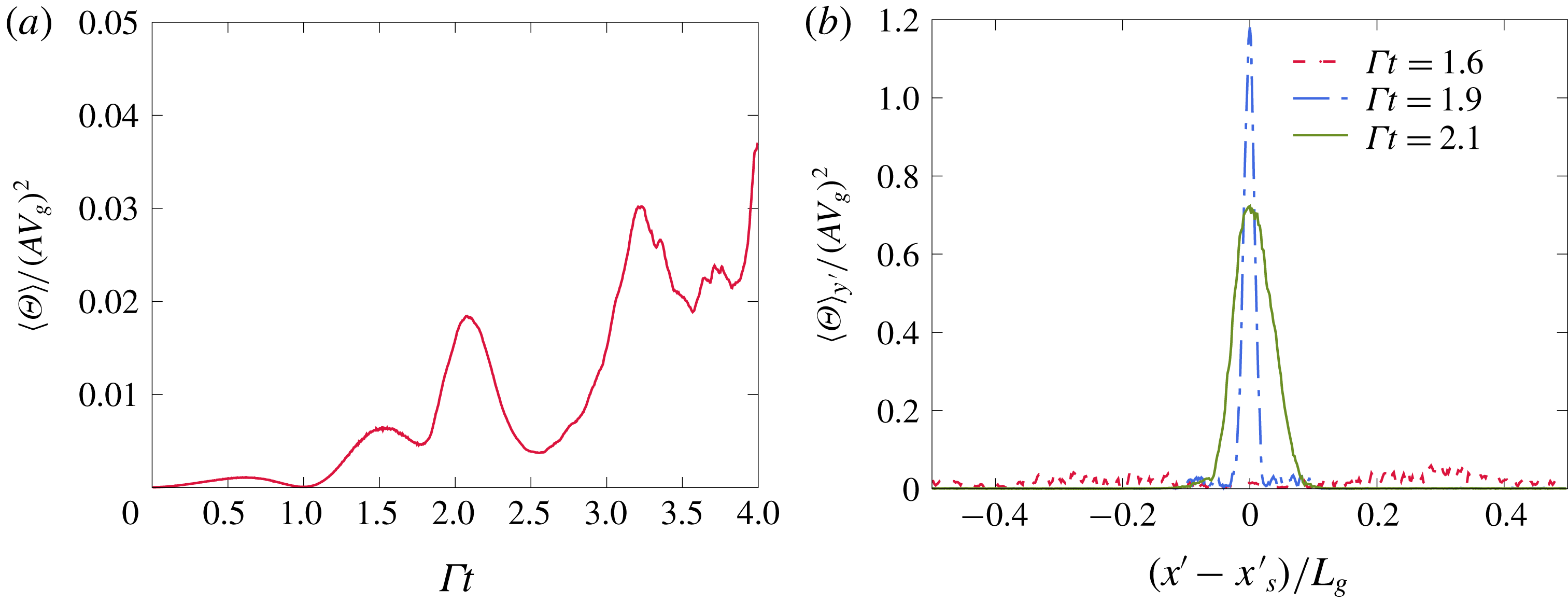
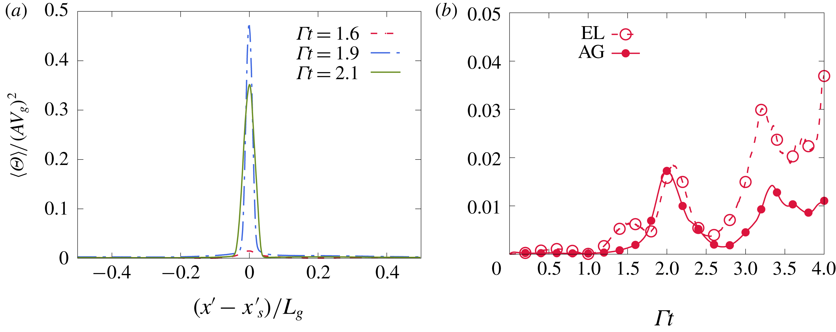
Granular temperature in the EL simulation. (a) Shows a peak of the domain-averaged granular temperature near the time caustics start appearing. (b) Shows the granular temperature peaks sharply at the location of the high concentration sheet of particles.
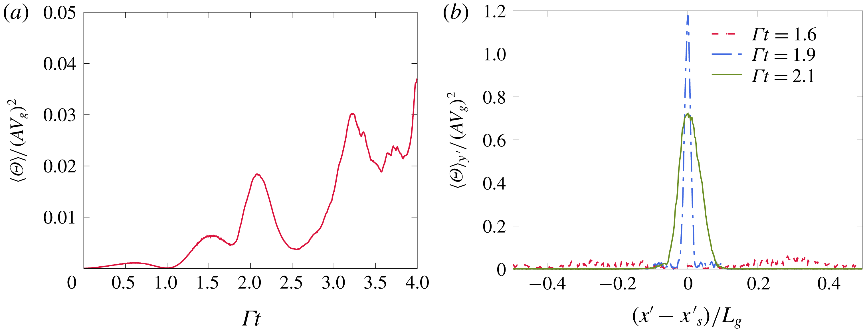
The spreading of the particle number density field by caustics effectively puts an end to the nonlinear amplification of the grid-resolved mean volume fraction variation due to preferential concentration. A quantitative measure of trajectory crossing is given by the granular temperature defined as the variance of the velocities of particles within a grid cell. Figure 11(a) shows that the domain-averaged granular temperature
 $\langle \unicode[STIX]{x1D6E9}\rangle$
reaches a peak around the same time
 $\unicode[STIX]{x1D719}_{rms}$
peaks. Furthermore, figure 11(b) shows this peak is spatially located near the region of particle crossing.
5.1.3 Rayleigh–Taylor instability
The nonlinear amplification of the preferential concentration instability triggers a transverse instability seen at
 $\unicode[STIX]{x1D6E4}t=2.325$
. The secondary instability happens on a time scale significantly shorter than that of the shear. As a result the one-dimensional wave resulting from the preferential concentration instability at
 $\unicode[STIX]{x1D6E4}t\sim 2$
can be considered a quasi-steady base state for the secondary instability. The shear forcing is negligible over the short duration of the development of the secondary instability and gravity is left as the sole driving force. To describe this secondary instability, we revert to a simpler formalism treating the particles and fluid as mixture. Using the expansion (2.20), one can show that a simplification of the governing equations of the particle-laden flow at a lower order in Stokes number yields the equations for a variable density fluid
 $$\begin{eqnarray}\displaystyle & \displaystyle \unicode[STIX]{x1D70C}_{m}\left(\frac{\unicode[STIX]{x2202}\boldsymbol{u}_{f}}{\unicode[STIX]{x2202}t}+\boldsymbol{u}_{f}\boldsymbol{\cdot }\unicode[STIX]{x1D735}\boldsymbol{u}_{f}\right)=-\unicode[STIX]{x1D735}p+\unicode[STIX]{x1D707}\unicode[STIX]{x1D6FB}^{2}\boldsymbol{u}_{f}+(\unicode[STIX]{x1D70C}_{m}-\unicode[STIX]{x1D70C}_{f})\boldsymbol{g}+O(\unicode[STIX]{x1D70F}_{p}), & \displaystyle\end{eqnarray}$$
 $$\begin{eqnarray}\displaystyle & \displaystyle \unicode[STIX]{x1D735}\boldsymbol{\cdot }\boldsymbol{u}_{f}=0, & \displaystyle\end{eqnarray}$$
 $$\begin{eqnarray}\displaystyle & \displaystyle \frac{\unicode[STIX]{x2202}\unicode[STIX]{x1D70C}_{m}}{\unicode[STIX]{x2202}t}+\boldsymbol{u}\boldsymbol{\cdot }\unicode[STIX]{x1D735}\unicode[STIX]{x1D70C}_{m}=O(\unicode[STIX]{x1D70F}_{p}), & \displaystyle\end{eqnarray}$$
where
 $\unicode[STIX]{x1D70C}_{m}=\unicode[STIX]{x1D70C}_{f}+\unicode[STIX]{x1D70C}_{p}\unicode[STIX]{x1D719}$
is the mixture density, and the preferential concentration terms are confined in the
 $O(\unicode[STIX]{x1D70F}_{p})$
terms. When completely neglecting the latter, the stability studies of unbounded variable density flows by Batchelor & Nitsche (Reference Batchelor and Nitsche1991) become of great relevance. Among the many base states they considered two of them are amenable to the configurations studied here: (i) sinusoidally varying density in the vertical direction, and (ii) long horizontal sheet of high density. Batchelor & Nitsche (Reference Batchelor and Nitsche1991) show that these configurations are subject to a Rayleigh–Taylor instability. Hence, to the extent that the quasi-steady flow and negligible preferential concentrations effects assumptions hold, the transverse secondary instability seen in figure 8 can be considered of a Rayleigh–Taylor type due to the mixture behaving as a variable density fluid.
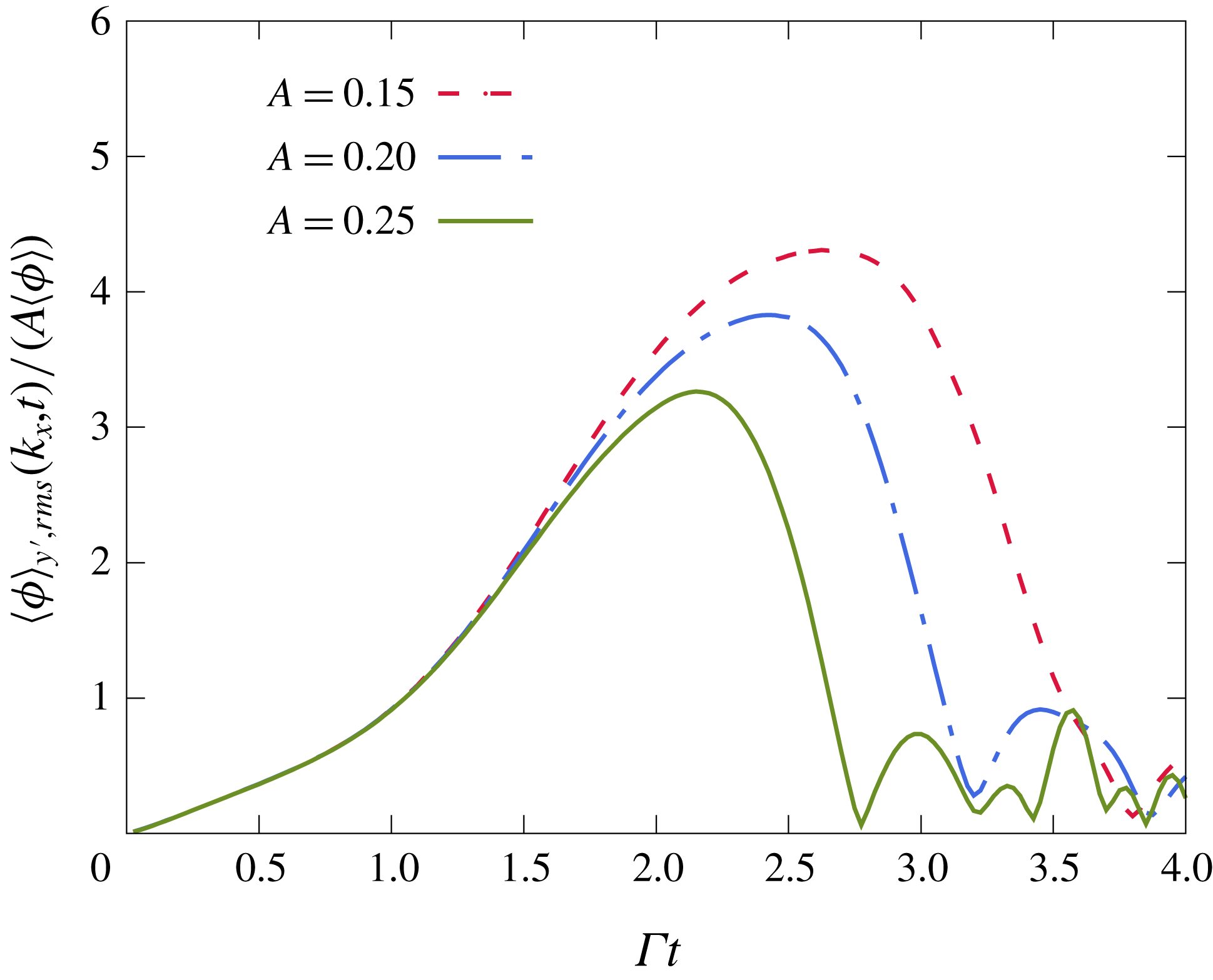
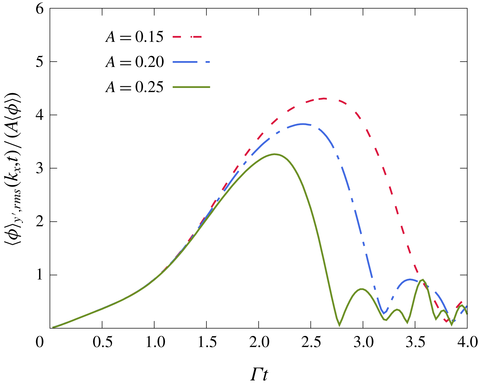
Evolution of mode
 $k_{x}^{\star }=1$
for the initial perturbation strengths
 $A=0.15$
, 0.20 and 0.25. The later decline of this mode for diminishing
 $A$
shows that the transverse perturbations are also delayed until a more favourable orientation and amplification are attained.
The results of Batchelor & Nitsche (Reference Batchelor and Nitsche1991) could be used to estimate the growth rate of the secondary modes. Case (i) might describe a transverse Rayleigh–Taylor instability growing at the early stages of the evolution of the mode
 $k_{x}^{\star }=1$
, i.e. while it remains sinusoidal. We focus on case (ii) since this is almost identical to the final stage of the nonlinear preferential concentration instability, around
 $\unicode[STIX]{x1D6E4}t=2$
, when the secondary Rayleigh–Taylor instability becomes evident. In the present case, the long band of particles is inclined rather than horizontal. Nevertheless, the results of the analysis of Batchelor & Nitsche (Reference Batchelor and Nitsche1991) can be used replacing the natural gravity by the effective wave-normal gravity
 $g_{n}=\Vert \boldsymbol{g}\boldsymbol{\cdot }\boldsymbol{k}\Vert /k=gk_{y}/k$
. To make use of the analysis, we will also assume a quasi-steady base state at
 $\unicode[STIX]{x1D6E4}t=2$
, meaning that the transverse perturbations grow on a time scale significantly smaller than
 $\unicode[STIX]{x1D6E4}^{-1}$
. Batchelor & Nitsche (Reference Batchelor and Nitsche1991) also assume that the transverse modes evolve in an inviscid fashion and have a wavelength much larger than the thickness of the band. Given these assumptions, a transverse mode with a wavenumber
 $\unicode[STIX]{x1D6FC}$
grows exponentially at the rate
 $$\begin{eqnarray}\unicode[STIX]{x1D70E}=\left(\frac{\unicode[STIX]{x03C0}}{2}\right)^{1/4}(\unicode[STIX]{x1D6FC}^{3}lg_{n}^{2})^{1/4}B^{1/2},\end{eqnarray}$$
where
 $l$
and
 $B$
represent the width and height of the mixture density impulse:
 $\unicode[STIX]{x1D70C}_{m}=\unicode[STIX]{x1D70C}_{f}(1+B\exp (-y^{2}/l^{2}))$
and
 $B\simeq \unicode[STIX]{x1D70C}_{p}/\unicode[STIX]{x1D70C}_{f}\unicode[STIX]{x1D719}_{max}-1$
. The ratio of time scales can be written in the following way:
 $$\begin{eqnarray}\frac{\unicode[STIX]{x1D70E}}{\unicode[STIX]{x1D6E4}}=\left(\frac{\unicode[STIX]{x03C0}}{2}\right)^{1/4}(\unicode[STIX]{x1D6FC}l)^{3/4}\sqrt{\frac{L_{g}}{l}\frac{k_{y}}{k}\frac{B}{St}}.\end{eqnarray}$$
The dependence on the inverse of the Stokes number shows that for small Stokes particles a quasi-steady assumption (
 $\unicode[STIX]{x1D70E}/\unicode[STIX]{x1D6E4}\gg 1$
) is valid. Expression (5.5) also shows that waves that achieve a more modest nonlinear growth by the preferential concentration instability, i.e. lower
 $B$
, will destabilize at an orientation closer to horizontal, i.e. larger
 $k_{y}/k$
. This trend is confirmed in figure 12 representing the evolution of the mode
 $k_{x}^{\star }=1$
for different initial strengths. The time at which this mode collapses indicates the time at which the transverse Rayleigh–Taylor instability appears. We see that for weaker initial strengths
 $A$
(and thus lower
 $B$
) the secondary instability is delayed, which allows the wave to further turn towards the horizontal.
The relation (5.5) can also be used to estimate the most likely transverse mode to grow. The scaling of the growth rate in
 $(\unicode[STIX]{x1D6FC}l)^{3/4}$
suggests that shorter wavelengths grow faster and the most likely mode to grow is such that
 $\unicode[STIX]{x1D6FC}l\sim 1$
. From figure 9(c), we estimate
 $l\simeq 0.05L_{g}$
,
 $B\simeq 17M\simeq 9.18$
and
 $k_{y}/k\simeq 0.67$
at
 $t=1.9$
. This gives a transverse wavelength
 $\unicode[STIX]{x1D706}_{RT}=2\unicode[STIX]{x03C0}/\unicode[STIX]{x1D6FC}\simeq 0.31L_{g}$
growing at the fast rate
 $\unicode[STIX]{x1D70E}\simeq 41\unicode[STIX]{x1D6E4}$
. The estimated wavelength is in agreement with the one seen in the snapshot at
 $\unicode[STIX]{x1D6E4}t=2.325$
in figure 8. The wavelength of the triggered mode in the transverse direction also depends on the strength of the initial perturbation driving the preferential concentration instability. Figure 13 shows that increasing the perturbation strength
 $A$
from 0.15 to 0.30 leads to the selection of larger wavelengths, in addition to triggering the instability earlier. A rigorous quantitative description of the most likely transverse perturbation to grow at finite Stokes number requires an analysis beyond the analogy made with the study of Batchelor & Nitsche (Reference Batchelor and Nitsche1991). In particular, the assumptions of quasi-steady base flow and infinitely small Stokes number behind expression (5.5) need to be relaxed.
Effect of varying the initial perturbation strength
 $A$
on the orientation and wavelength of the transverse mode.
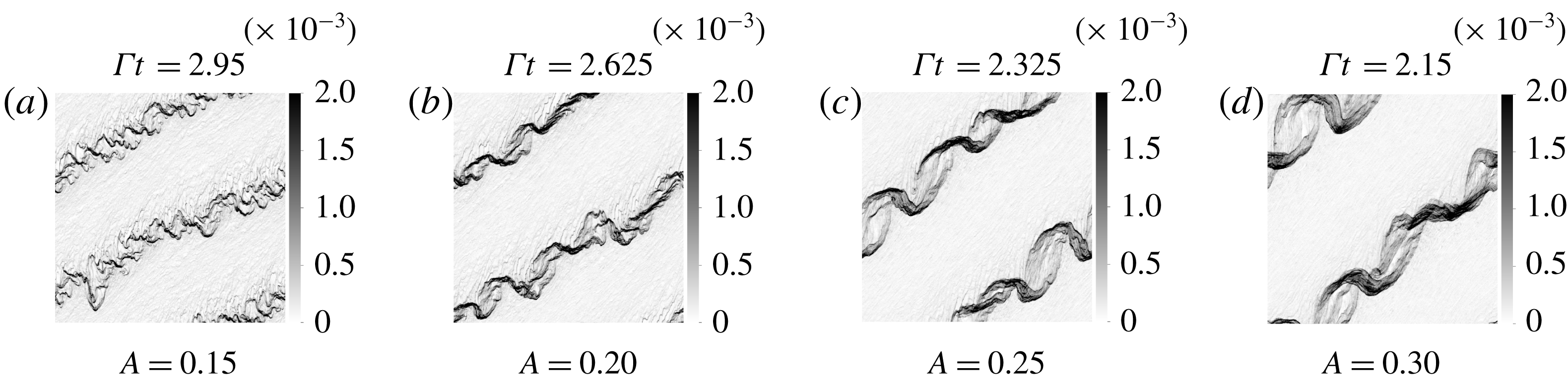
5.2 Nonlinearities in EE formulations
Having described in detail the nonlinear dynamics revealed in Euler–Lagrange (EL) simulations, we now turn to consider the fidelity with which Euler–Euler formulations capture these effects. In particular, we show results of the two-fluid equations (TF) which consider the particle velocity field to be single valued and the anisotropic-Gaussian (AG) model that allows for multiplicity of particle velocities in a single grid cell. The preferential concentration instability in these simulations is seeded with a fluid velocity perturbation of strength
 $A=0.25$
as in the EL simulations. Some small perturbation with variations normal to the imposed wave vector is required to trigger secondary instabilities. In the EL simulations, these perturbations were provided by the initial random distribution of particle positions. To provide a close comparison with this case we initialize the EE simulations with a volume fraction field computed based on grid cell averages of the initial discrete particle distribution used in EL simulations.
Snapshots of the volume fraction field in TF simulation at
 $A=0.25$
.
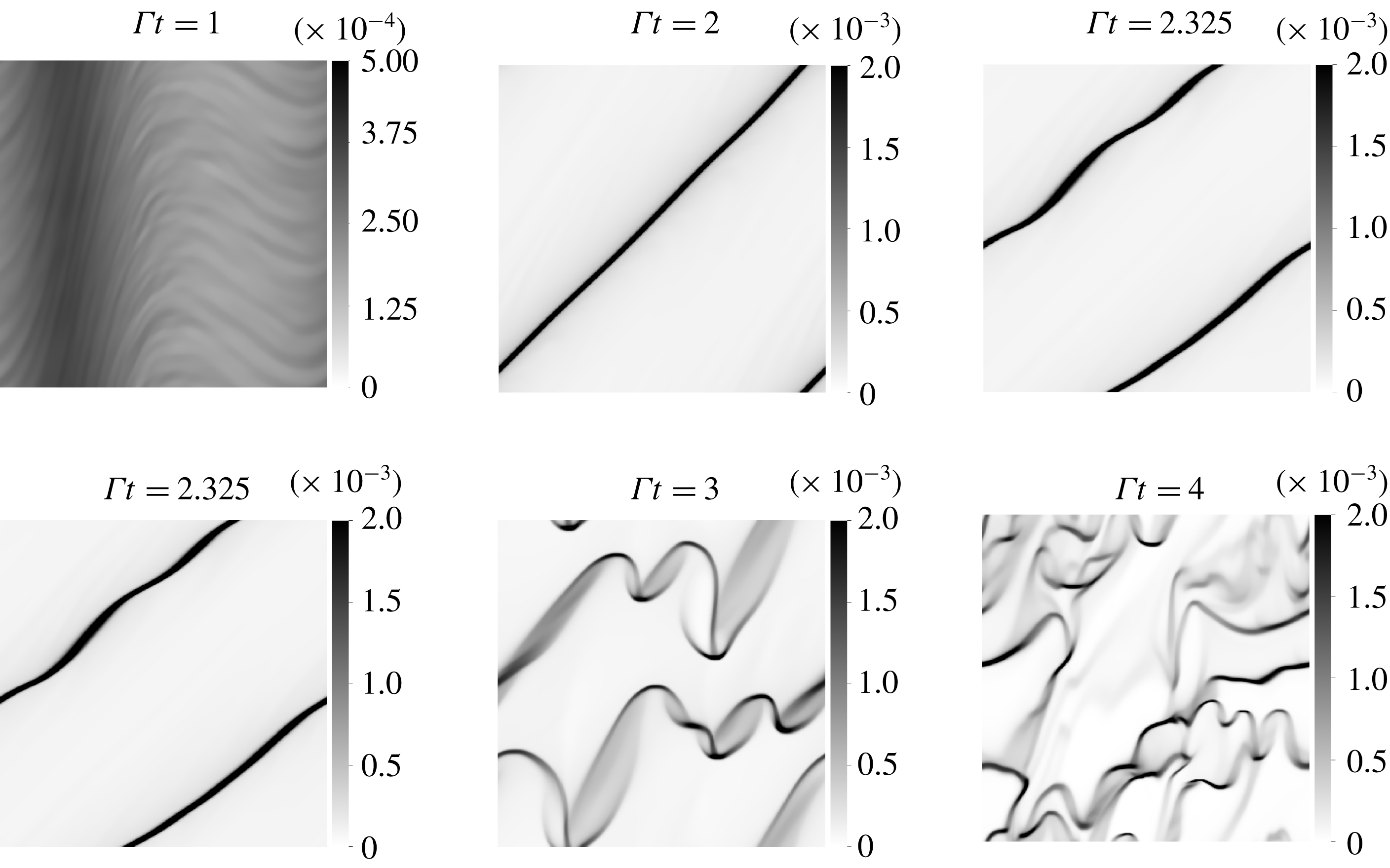
Snapshots of the volume fraction field in AG simulation at
 $A=0.25$
.
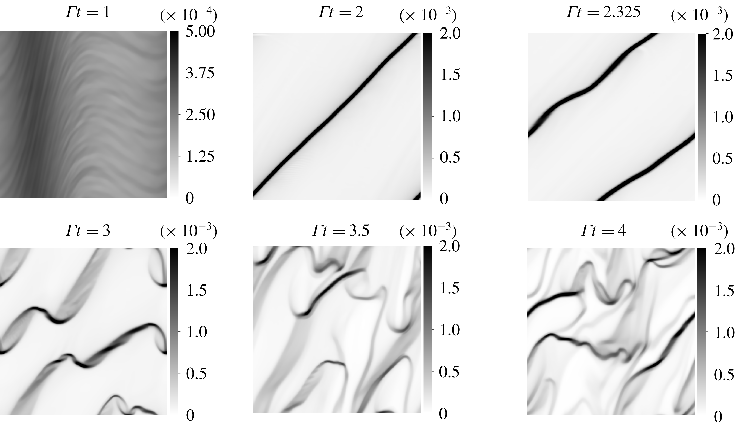
The nonlinear perturbation triggers the same qualitative dynamics in all three simulation approaches. The snapshots of volume fraction, shown in figures 14 and 15 for TF and AG simulations depict similar dynamics as shown in figure 8 for EL simulations: the initially sinusoidal wave of volume fraction sharpens into a highly concentrated particle sheet, which becomes unstable at
 $\unicode[STIX]{x1D6E4}t\sim 2.3$
to a transverse Rayleigh–Taylor instability leading eventually to a state of sustained clustering. The r.m.s. of the volume fraction over the entire cell grows nonlinearly and peaks at
 $\unicode[STIX]{x1D6E4}t\sim 2$
in all three methodologies (see figure 16).
Evolution of the volume fraction fluctuations in the three simulation methods.
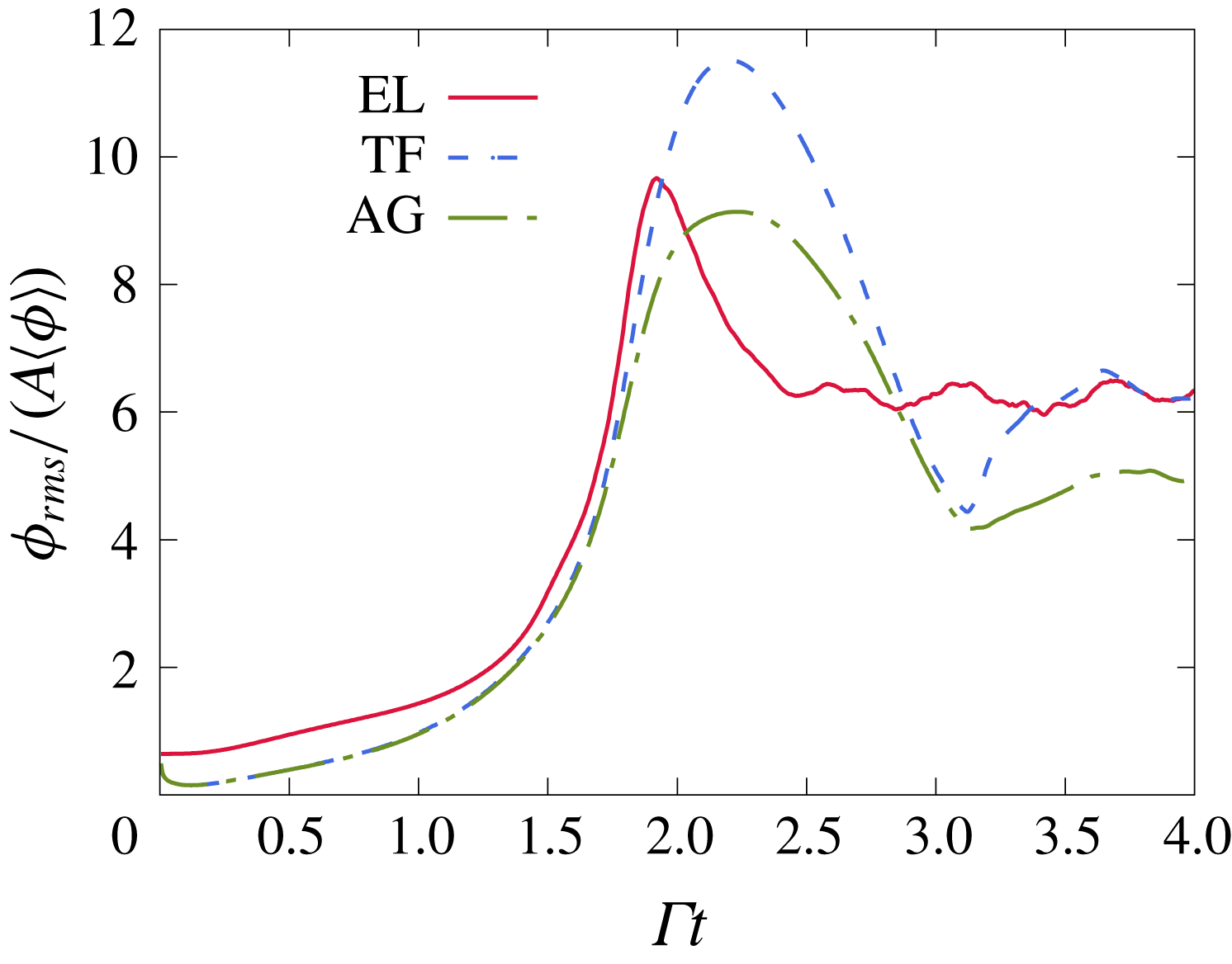
While AG and TF simulations lead to a chain of mechanisms similar to the one analysed for EL simulations in § 5.1, the particle sheet developed at
 $\unicode[STIX]{x1D6E4}t=2.1$
and the clusters developing by
 $\unicode[STIX]{x1D6E4}t=4$
are finer with higher local concentration in the TF simulations. This behaviour can be linked to the effects of particle-trajectory crossing. The TF method used here is based on a mono-kinetic assumption whereby all particle velocity vectors are equal within one grid cell. Thus it does not capture particle-trajectory crossing. Without the dispersive effect of particle-trajectory crossing, particle concentrations can become very large and particle velocity fields can become nearly discontinuous in space limited only by a slope limiting condition applied in the numerical evaluation of the TF model. Figure 17(b) shows the wave-normal velocity for the times
 $\unicode[STIX]{x1D6E4}t=1.6,$
1.9 and 2.1 in TF and EL simulations. One can see that both methods collapse at the two earliest times during the wave steepening. However, at
 $\unicode[STIX]{x1D6E4}t=2.1$
the velocity profile broadens in the EL simulation as a result of trajectory crossing, while the TF velocity profile retains a large gradient. The shock-like wave normal velocity profile in the TF method leads to a sharp volume fraction impulse as seen in figure 17(a). In contrast, the wave-normal velocity profile broadens in the AG method by
 $\unicode[STIX]{x1D6E4}t=2.1$
in qualitative agreement with the EL simulations as seen in figure 17(d). This results in a spread out volume fraction profile in AG simulations at
 $\unicode[STIX]{x1D6E4}t=2.1$
(figure 17
c) as in EL simulations, although this profile appears smoother likely due to limited numerical resolution.
A key element in removing the discontinuity in AG is the incorporation of a poly-kinetic sub-grid model for the particle number density pdf controlled by the particle pressure tensor. The trace of the latter, i.e. the granular temperature, is seen to reach a high peak at the particle sheet location in figure 18(a). Despite differences in the magnitudes reached in AG and EL simulations, the trends are qualitatively similar. In particular, the time for the onset of significant granular temperature indicative of trajectory crossing is
 $\unicode[STIX]{x1D6E4}t\sim 2$
in both AG and EL simulations as seen in the plot of the domain-averaged granular temperature in figure 18(b).
Thus, the AG method reproduces all the major aspects of the nonlinear state seen in the EL simulations as outlined in § 5.1: the nonlinear growth and sharpening of the wave due to the preferential concentration, particle-trajectory crossing and the secondary Rayleigh–Taylor instability. The most striking difference between the AG and EL results seen by comparing figures 15 and 8 is the presence of smaller wavelength features in the EL simulations. This is seen both during the onset of the secondary instability at
 $\unicode[STIX]{x1D6E4}t\sim 2$
–2.3 and the final clustered state at
 $\unicode[STIX]{x1D6E4}t=4$
. The fine-scale features in the EL simulations can be attributed in part to initial sub-grid-scale particle volume fraction fluctuations captured by the randomly distributed particles in the EL formulation which eventually influence the grid-averaged structure. In addition, EE methods by their nature exhibit numerical diffusion of resolved small-scale volume fractions while the EL method is able to retain small-scale volume fractions through the initial growth period so that they can participate in the later time
 $\unicode[STIX]{x1D6E4}t\geqslant 2$
dynamics.
Volume fraction and wave-normal velocity as function of the centred wave-normal coordinate in TF (a,b) and AG (c,d) simulations. The inability of the TF method to resolve particle-trajectory crossing leads to a higher volume fraction peak (a) and steeper wave-normal velocity (b) than in EL at
 $\unicode[STIX]{x1D6E4}t=2.1$
. The assumption of anisotropic-Gaussian particle number density pdf leads to a spread out volume fraction field (c) and lower gradient of the wave-normal velocity (d) at
 $\unicode[STIX]{x1D6E4}t=2.1$
than in TF.

Granular temperature in AG simulations. Similarly to EL, graphs of the granular temperature in the wave-normal direction (a) display a sharp peak at the particle sheet location, although lower to the one observed in EL. The domain-averaged granular temperature (b) in AG and EL display qualitatively similar evolutions. The peak at
 $\unicode[STIX]{x1D6E4}t\sim 2$
due to the two particle streams crossing at the high concentration band is well reproduced in AG.

6 Conclusion
An investigation of clustering in homogeneously sheared particle-laden flow in the two-way coupling regime reveals a ‘route to clustering’ that involves three mechanisms leading to a state of significant clustering. Perturbations of the particle and fluid velocities induce inhomogeneities in the particle distribution by the preferential concentration mechanism. In the presence of shear, these perturbations grow algebraically by a two-way mechanism that is promoted by preferential concentration and gravity. This first stage in the ‘route to clustering’, leads to the accumulation of particles on fine sheets with a concentration about 18 times higher than the average. When the local volume fraction reaches high magnitudes (
 ${>}10^{-3}$
), particle-trajectory crossing leads to a local dispersion of particles due to the formation of caustics. This also induces a spreading of the high concentration sheets. Finally, the turning of the sheets by the shear towards the horizontal leads to the appearance of a secondary Rayleigh–Taylor instability. The transverse perturbations breaks the particle sheet into smaller clusters. In the final stages of the simulations, these particle structures continue to sharpen and break repeatedly. These structures traverse each other and only interact through their coupling with the fluid.
The simulations were conducted in the Euler–Lagrange and Euler–Euler formulations with a methodology that emulates the unboundedness of homogeneous shear. The use of the shear-periodic boundary conditions allows the forcing of fluctuations by the linear homogeneous shear without the introduction of confining scales, such as in mixing layers or wall-driven shear. This allows the accurate description of the rotation of Fourier modes by the shear. The evolution of these modes in the linear regime was described in a prior study (Kasbaoui et al. Reference Kasbaoui, Koch, Subramanian and Desjardins2015) using a two-fluid representation of the two phases. Full nonlinear simulations with two Euler–Euler methods, the two-fluid and anisotropic-Gaussian methods, show agreement with Euler–Lagrange simulations and the linear stability analysis for small Stokes number particles, as long as the particle distribution inhomogeneities remain small.
In presence of strong clustering characterized by large void regions and highly concentrated particle structures, differences in the Euler–Lagrange and Euler–Euler methods emerge. The two-fluid method relying on a mono-kinetic description of the local particle velocity pdf lead to the formation of discontinuities at the high concentration sheets. The volume fraction across these sheets takes the shape of an impulse. The particle velocity across the sheet steepens from a sinusoidal function to a nearly step function. Particle-trajectory crossing in Euler–Lagrange simulations removes the discontinuity. The crossing of two streams of particle coming from both sides of the sheet of particles leads to the spreading of the volume fraction field around the sheet and lower gradients. This poly-kinetic behaviour is approximated in the anisotropic-Gaussian method which models the sub-grid particle number density pdf with an anisotropic-Gaussian distribution. In particular, the particle-trajectory crossing at the particle sheet is reproduced with this Eulerian method. The granular temperature, a measure of particle-trajectory crossing, is reproduced qualitatively.
Acknowledgements
This work was supported by NSF grants CBET-1233793 and CBET-1505759.