1. Introduction
With the steady advancement of Industry 4.0 and intelligent manufacturing, there is an increasing demand for efficient, precise, intelligent, and flexible automation equipment in industrial production [Reference Bogue1–Reference Meike and Ribickis2]. Under this background, industrial robot technology is progressing rapidly and becoming fully integrated across various industries. As a crucial intelligent component of industrial robots, parallel robots differ greatly from their serial counterparts. They are typically composed of multiple closed-loop branches. Their passive arms have a relatively simple and symmetric structure, and their workspace is usually regular in shape, making their overall structure more compact. In contrast, serial robots have joints connected in sequence, which can result in significant cumulative errors at the end effector. Parallel robots, leveraging the synergistic operation of multiple kinematic chains, achieve superior motion accuracy and greater stiffness. This design enables the moving platform to remain stable even in confined spaces [Reference Badrikouhi and Bamdad3–Reference Sun, Li, Wang, Chen, Chen, Zeng, Zhao and Yue4]. Parallel robots have demonstrated exceptional performance in the fields such as food sorting, precision electronic assembly, and high-speed logistics handling, making them an area of significant research interest [Reference Zhou and Yu5].
The design and innovation of low-degree-of-freedom (DOF) parallel robots have long been a focal point in robotics research. Through extensive investigation and exploration, numerous scholars have made significant advances in the design, structural innovation, kinematics and dynamics analysis, and optimal control of parallel robots. Shen et al. [Reference Shen and Yang6] proposed a waterbomb-structure-inspired hybrid mechanism for a soft crawling robot using thick-panel origami, inspiring hybrid structure design in robotics. Researchers such as Gosselin and Angeles [Reference Gosselin and Angeles7–Reference Gosselin and Angeles9] have laid the theoretical foundation for the field by conducting preliminary studies on the kinematics and mechanical characteristics of parallel robots. Gallardo Alvarado Jaime [Reference Gallardo-Alvarado10] introduced a simplified matrix method in his research to balance forces and moments in planar parallel manipulators. The Delta parallel robot, introduced by professor Clavel, is capable of achieving 3-DOF translational motion in space, which has significantly contributed to the widespread application of parallel robots in packaging, material handling, and medical fields. Building upon the Delta parallel robot, many scholars have further investigated and proposed designs for parallel robots with various DOFs tailored to specific working environments and production tasks. For instance, the Diamond parallel robot developed by Huang et al. [Reference Yang, Wu, Mei, Jian and Huang11] features two translational DOFs and offers high rigidity and precision through an innovative hinge design, making it well-suited for applications requiring high dynamic performance and precision control. Xu et al. [Reference Xu, Xie, Yang, Zhao and Wang12] proposed a 2-DOF rotational spatial parallel mechanism for end effector control in narrow spaces and established its forward and inverse kinematics models via pose constraints and the closed vector method. French scientist Pierrot introduced a double-movable structure for the moving platform, leading to the development of a series of parallel robots capable of achieving 3T1R motions, such as Heli4 [Reference Krut, Company, Nabat and Pierrot13] and Part4 [Reference Nabat, de la O. Rodriguez, Company, Krut and Pierrot14]. Liu et al. [Reference Xie and Liu15–Reference Mo, Shao, Guan, Xie and Tang16] further proposed the 4-DOF X4 parallel robot, utilizing a symmetric configuration of the moving platform and branches. Additionally, Li et al. [Reference Meng, Gao, Wu and Ge17], employing Lie group theory, developed various symmetric structures for low-DOF parallel robots. Shen et al. [Reference Shen, Xie, Song and Bao18] designed a parallel four-legged robot, conducted kinematic analysis of one of its legs, and further extended this analysis to all four legs. With the continuous improvement of intelligent and automated production levels, product handling and packing operations impose special requirements on the performance of industrial robots. Such production operations often require robots to complete operations such as grabbing, placing, and handling within a plane. Therefore, carrying out the design and research on two-translational parallel robots is of great theoretical research significance for promoting the innovative development of the robot industry.
Rigid body dynamics modeling is a critical technology for parallel robots. Through accurate modeling, the mechanical properties of the robot can be deeply analyzed, enabling precise motion planning and control, thereby improving overall performance and efficiency. Currently, commonly used methods for dynamic modeling of parallel robots include the virtual work principle [Reference Zhao and Gao19], Kane’s method [Reference Talaeizadeh, Forootan, Zabihi and Pishkenari20], Lagrange’s method [Reference Lin and Zhang21], and the Newton–Euler method [Reference Chen, Nie, Meng, Chen, Jia and Pan22–Reference Huang, Han, Li, Xu and Wu23]. The virtual work principle, which is based on an energy perspective, avoids the need for complex force analysis, reducing the complexity of modeling and streamlining the process. This method allows for accurate and efficient determination of joint forces and motion parameters, making it widely adopted for dynamic modeling of parallel robots globally. Wang et al. [Reference Wang, Yang, Zhang, Fang, Lai, Feng, Wei and Wang24] proposed an improved method for analyzing the non-inertial dynamics of the 3-SPS/U parallel platform. By combining Kane’s method with screw theory, they extended the traditional inertial dynamics analysis to the non-inertial frame. Hou et al. [Reference Hou, Zhang and Zeng25] established a dynamic model of Stewart parallel manipulators based on screw theory and verified the dynamic model through dynamic simulation using MSC-Adams software. Huang et al. [Reference Huang, Zhang, Xiong and Liu26] derived the centroid inertial force equations of each connecting rod using the Newton–Euler method, analyzed the causes of over-constraints by applying screw theory, and introduced the elastic deformation of the connecting rods as a supplement to the deformation compatibility equations, thus completing the modeling of the 4-DOF over-constraint parallel robot.
Dimension synthesis is a crucial aspect of parallel robot design, playing an indispensable role in determining the performance of the mechanism. The dimensional parameters have a significant impact on the working performance of the robot. Currently, research on mechanism dimension synthesis is primarily focused on the kinematics level, with commonly used objective functions including the condition number of the velocity Jacobian matrix [Reference Kim27–Reference Li and Angeles28], dexterity [Reference Liang, Zeng, Li, Su and He29–Reference Deng, Zhang and Yan30], and maximum and minimum singular values of the velocity Jacobian matrix [Reference Pulloquinga, Escarabajal, Valera, Valles and Mata31–Reference Jian-she, Ming-xiang, Yu-Yin and Bao-tang32] of the Jacobian matrix, which are optimized to obtain the optimal dimensional parameters. Cui et al. [Reference Cui, Zhang, Zhou and Zhang33] studied the operational dexterity and multiobjective optimization of a 3-DOF parallel robot used in the segment assembly system of a shield machine. Brinker et al. [Reference Brinker, Corves and Takeda34] conducted dimensional synthesis of the Delta parallel robot based on its motion/force transmission characteristics. As robot’s speed and acceleration increase, the dynamic characteristics of the parallel robot become crucial in the dimensional synthesis process. However, most existing research on rigid body dynamics-based dimensional synthesis tends to focus on single-factor consideration, leaving room for improvement in the overall optimization of robot performance. Huang et al. [Reference Huang, Liu, Mei and Chetwynd35] took into account two performance evaluation indices, namely, normalized inertia and the centrifugal or Coriolis moment dynamics of a single driving joint, and employed two types of pressure angles as kinematic constraints to perform dimensional synthesis of a planar 2-DOF parallel manipulator. Liu et al. [Reference Liu, Huang, Mei, Zhao, Wang and Chetwynd36] conducted an in-depth analysis of both the kinematic and dynamic characteristics, leading to the optimized design of a 4-DOF Scara parallel robot. Despite considerable research on dynamic dimensional synthesis and kinematic performance optimization, the study of dimensional synthesis that integrates both kinematic and dynamic characteristics remains limited.
Based on the concept of modular design, this paper proposes and analyzes a modular parallel robot with multi-DOF capability. The kinematics and rigid body dynamics models of the parallel robot are developed using the vector analysis method and the principle of virtual power. The dynamic dimensional synthesis problem is then systematically addressed through a multiobjective optimization approach. Additionally, the control of the physical prototype of the parallel robot is explored.
In contrast to the previous investigations, the main contributions of this paper are summarized as follows:
-
• A novel two-translational parallel robot is proposed. This robot employs over-constraint to enhance structural stiffness and improve motion stability. Moreover, two types of auxiliary modules are constructed according to the production tasks. Through the coordinated cooperation of each module, the robot can have multiple DOF modes, thereby enhancing the multi-task applicability of the robot.
-
• A dimensional synthesis model that takes into account both kinematic and dynamic performances is constructed. Based on this model, an optimization analysis of the robot is carried out, and a set of optimal dimensional parameters is obtained.
-
• A physical prototype of the parallel robot was built, and open-loop control experiments were carried out.
The remainder of this paper is organized as follows. The logical framework of this paper is illustrated in Figure 1. Section 2 presents the design concept of the proposed mechanism and analyzes its DOF. In Section 3, the kinematics of the parallel robot is examined, and both the forward and inverse kinematics solutions, along with the mapping relationships for velocity and acceleration, are derived. Section 4 establishes the rigid body dynamics model of the parallel robot, with the model’s validity confirmed through multi-body simulation software. In Section 5, the dynamic dimensional synthesis problem is analyzed, and a multiobjective optimization method that considers both kinematic and dynamic performance is proposed for dimensional synthesis. Section 6 details the construction of the physical prototype and the control performance tests conducted on the prototype. Finally, conclusions are drawn in Section 7.
Paper structure diagram.

2. Design and DOF analysis of the parallel robot
2.1. Mechanism design
To address the high-speed and high-load demands of parallel robots in complex environments, this paper presents the design and conceptual framework of a novel multi-DOF modular parallel robot. Figure 2(a) depicts the robot, which possesses two translational DOFs. The static platform is shaped as an isosceles trapezoid. This spatial arrangement enhances the stiffness of the mechanism without altering its planar two-DOF nature. A servo motor is coupled to each linear module, enabling the lead screw to rotate in conjunction with the motor, thereby driving the slider in a linear reciprocating motion. Two connecting frames are attached to these sliders and interface with the moving platform via two passive limbs. Each connecting frame, together with a passive limb and one side of the moving platform, collectively forms a spatial 4U closed-loop subchain (where U denotes a Hooke joint), resulting in a spatial isosceles trapezoid structure. The assembly of the parallel robot is completed by linking the four passive limbs to their respective connecting frames and the moving platform.
Initial configuration of the parallel robot and arrangement of its branches. (a) The principal framework. (b) Side view of the principal framework. (c) Schematic diagram of long-distance transportation module. (d) Schematic diagram of the central flipping module.

Building upon the original mechanism, this paper introduces an auxiliary module that, through coordinated operation with the base structure, enables a multi-DOF mode for the parallel robot. To increase the number of DOFs, a modular design approach was adopted to construct two additional modules: a long-distance horizontal transportation module (Figure 2(c)) and a horizontal flipping module (Figure 2(d)). The long-distance transportation module primarily consists of a ball screw and two parallel optical axis guides mounted above the robot’s frame. This configuration allows the parallel robot and the transportation module to operate synergistically, achieving 3-DOF translational motion. The horizontal flipping module comprises a central servo motor and a UPU (Universal-Prismatic-Universal) limb, installed on the lower section of the static platform. The central servo motor drives the end effector to perform a full-cycle rotation about its axis, thereby enabling the flipping of grasped workpieces in practical production tasks.
Since the UPU branch (with p denoting a passive prismatic pair) in the horizontal flipping module is only used to realize the decoupled rotational motion of the end effector – and as the module’s central servo drive motor solely drives this rotational motion, the UPU branch itself does not interfere with the motion of other branches or the translational motion of the moving platform – it can serve as an auxiliary module and be installed according to specific application requirements. Therefore, the subsequent analysis will only focus on the main part of the robot (i.e., the principal framework, as shown in Figure 2(a)).
The modular robot with a multi-DOF mode is developed by Tiangong University (abbreviated as TGU). A key feature of this robot is that the passive arm branch of the parallel robot adopts a spatial V-shaped configuration, while the main parallel robot allows for 2-DOF translational motion. As a result, this translational parallel robot is named TGU-SV2. The robot is cost-effective to manufacture, owing to its simplified mechanical architecture comprising only two linear drive modules, four driven links, and a moving platform – fewer components reduce material expenses, machining complexity, assembly time. It is also easy to control, as it uses only two servo motors (reducing control input dimensionality) and features simplified forward/inverse kinematic models that lower computational burdens for trajectory planning and control algorithms. With such attributes, the TGU-SV2 has promising application potential in high-speed operations, such as industrial production and logistics sorting. Given that the TGU-SV2 parallel robot forms the core structure of the robot, with the other modules serving as auxiliary components, the focus of this paper is on the kinematics and dynamics modeling, optimization design, prototype construction, and testing of the TGU-SV2 parallel robot.
2.2. Analysis of the DOF of the parallel robot
The TGU-SV2 parallel robot is composed of two symmetrical branches, each consisting of a linear drive module and a 4U closed-loop subchain, where “U” represents a Hooke joint. Analyzing the configuration of the mechanism reveals that it is an over-constrained system. Over-constrained mechanisms are special types of mechanisms that do not satisfy the Kutzbach criterion for determining the DOFs. The traditional Gruebler–Kutzbach (G–K) formula fails to precisely ascertain the type and quantity of DOFs for this mechanism. To address this issue, this paper uses screw theory to analyze the DOFs of the parallel robot, thereby clarifying the quantity and nature of its DOFs.
As shown in Figure 3, the analysis is conducted in an inertial coordinate system, where the axis
 ${\textit y}$
aligns with the direction of motion
 ${\textit O}{\textit A}_{1}$
, and the axis
 ${\textit z}$
always maintains a vertical upward orientation. The axis x follows the right-hand rule for the direction of rotation.
Screw vector diagram of TGU-SV2 parallel robot.

Given the symmetry and identical configuration of the left and right branches of the parallel robot, without loss of generality, the left single branch is selected for analysis. Based on the inertial coordinate system
 ${\textit O}\mathit{-}{\textit xyz}$
, the motion screws of the single-branch chain are analyzed. Thus, it can be derived that
 $\boldsymbol{\$ }_{{\textit i}}({\textit i}=1,2)$
denotes the motion screw of the prismatic pair, while the screws associated with the Hooke’s joints are explicitly illustrated at their corresponding positions within the diagram.
The analysis of the screw diagram of the single branch chain reveals that the motion screw of the prismatic pair
 ${\textit A}_{2}{\textit B}_{2}$
is
 \begin{equation} \boldsymbol{\$ }_{2}=\left(\begin{array}{lll} \begin{array}{llll} 0 &\quad 0 &\quad 0 &\quad 0 \end{array} &\quad {\textit e}_{2} &\quad {\textit f}_{2} \end{array}\right) ^{\mathrm{T}}\end{equation}
where
 ${\textit e}_{2}$
and
 ${\textit f}_{2}$
represent values of the motion screw of the prismatic pair in the y-direction and z-direction, respectively.
Based on the same reference coordinate system, the 4U closed-loop subchain is analyzed. The 4U closed-loop branch can be considered as a parallel mechanism composed of two U-U branches,
 ${\textit E}_{2}{\textit F}_{2}$
and
 ${\textit E}_{4}{\textit F}_{4}$
. Due to the symmetry of the
 ${\textit E}_{2}{\textit F}_{2}$
and
 ${\textit E}_{4}{\textit F}_{4}$
branches, when calculating the constraint screw system of
 ${\textit E}_{2}{\textit F}_{2}$
and
 ${\textit E}_{4}{\textit F}_{4}$
, the screws with
 ${\textit k}=1$
in the
 ${\textit E}_{2}{\textit F}_{2}$
branch and the screws with
 ${\textit k}=-1$
in the
 ${\textit E}_{4}{\textit F}_{4}$
branch are recorded. Without loss of generality, the
 ${\textit E}_{2}{\textit F}_{2}$
branch is analyzed in detail.
For convenience in analysis, denote the axis vector of the first U-pair fixed shaft in the
 ${\textit E}_{2}{\textit F}_{2}$
branch as
 $\boldsymbol{\omega }_{21}=[\begin{array}{lll} {\textit k}{\textit l}_{1} & \ \ {\textit m}_{1} & \ \ 0 \end{array}]$
(with
 ${\textit k}=1$
, and the same notation applies below). The axis vector of its oscillating shaft is
 $\boldsymbol{\omega }_{22}=[\begin{array}{lll} {\textit k}{\textit l}_{2} & \ \ {\textit m}_{2} & \ \ {\textit n}_{2} \end{array}]$
, and the position vector of its center point
 ${\textit E}_{2}$
is
 ${\textit r}_{\mathrm{E}2}=[\begin{array}{lll} {\textit k}\overline{{\textit x}}_{1} & \ \ \overline{{\textit y}}_{1} & \ \ \overline{{\textit z}}_{1} \end{array}]$
. Similarly, denote the axis vector of the second U-pair fixed shaft in the
 ${\textit E}_{2}{\textit F}_{2}$
branch as
 $\boldsymbol{\omega }_{41} = \boldsymbol{\omega }_{21}$
, the axis vector of its oscillating shaft as
 $\boldsymbol{\omega }_{42} = \boldsymbol{\omega }_{22}$
, and the position vector of the center point
 ${\textit F}_{2}$
is
 $\boldsymbol{r}_{\mathrm{F}2}=[\begin{array}{lll} {\textit k}\overline{{\textit x}}_{2} & \ \ \overline{{\textit y}}_{2} & \ \ \overline{{\textit z}}_{2} \end{array}]$
. Then, the kinematic screw system of the
 ${\textit E}_{2}{\textit F}_{2}$
branch is
 \begin{equation} \tilde{\boldsymbol{W}}_{2}=\begin{cases} \boldsymbol{\$ }_{21}=\big(\begin{array}{ll} \boldsymbol{\omega }_{21}; &\quad \boldsymbol{r}_{\mathrm{E}2}\times \boldsymbol{\omega }_{21} \end{array}\big)\\[3pt]\boldsymbol{\$ }_{22}=\big(\begin{array}{ll} \boldsymbol{\omega }_{22}; &\quad \boldsymbol{r}_{\mathrm{E}2}\times \boldsymbol{\omega }_{22} \end{array}\big)\\[3pt]\boldsymbol{\$ }_{41}=\big(\begin{array}{ll} \boldsymbol{\omega }_{41}; &\quad \boldsymbol{r}_{\mathrm{F}2}\times \boldsymbol{\omega }_{41} \end{array}\big)\\[3pt] \boldsymbol{\$ }_{42}=\big(\begin{array}{ll} \boldsymbol{\omega }_{42}; &\quad \boldsymbol{r}_{\mathrm{F}2}\times \boldsymbol{\omega }_{42} \end{array}\big) \end{cases} \end{equation}
Based on the concept and algorithm of the screw reciprocal product [Reference Liang, Mao, Song, Chang and Sun37], the inverse screw of Eq. (2) is derived, resulting in the constraint screw system for the branch, as follows:
 \begin{equation} \begin{cases} {\boldsymbol{\$ }}_{21}^{\mathrm{r}}=\left(\begin{array}{lll} 0 &\quad 0 &\quad \begin{array}{lll} 0 &\quad \dfrac{\textit{km}_{1}\textit{n}_{2}}{\textit{w}_{1}} &\quad \begin{array}{ll} -\dfrac{\mathrm{l}_{1}\mathrm{n}_{2}}{\mathrm{w}_{1}} &\quad 1 \end{array} \end{array} \end{array}\!\!\right)^{\mathrm{T}}\\[7pt] {\boldsymbol{\$ }}_{22}^{\mathrm{r}}=\left(\begin{array}{lll} \dfrac{\textit{k}\left(\overline{\textit{x}}_{1}-\overline{\textit{x}}_{2}\right)}{\left(\overline{\textit{z}}_{1}-\overline{\textit{z}}_{2}\right)} &\quad \dfrac{\left(\overline{\textit{y}}_{1}-\overline{\textit{y}}_{2}\right)}{\left(\overline{\textit{z}}_{1}-\overline{\textit{z}}_{2}\right)} &\quad \begin{array}{llll} 1 &\quad -\dfrac{\textit{w}_{2}}{\left(\overline{\textit{z}}_{1}-\overline{\textit{z}}_{2}\right)\textit{w}_{1}} &\quad \dfrac{\textit{kw}_{3}}{\left(\overline{\textit{z}}_{1}-\overline{\textit{z}}_{2}\right)\textit{w}_{1}} &\quad 0 \end{array} \end{array}\!\right)^{\mathrm{T}} \end{cases} \end{equation}
The expressions for
 $\textit{w}_{1} , \textit{w}_{2}$
, and
 $\textit{w}_{3}$
are as follows:
 \begin{equation*} \begin{array}{l} \textit{w}_{1}=\textit{l}_{1}\textit{m}_{2}-\textit{l}_{2}\textit{m}_{1},\textit{w}_{2}=(\textit{l}_{1}\textit{m}_{2}-\textit{l}_{2}\textit{m}_{1})(\overline{\textit{y}}_{1}\overline{\textit{z}}_{2}-\overline{\textit{y}}_{2}\overline{\textit{z}}_{1})-\textit{m}_{1}\textit{n}_{2}(\overline{\textit{x}}_{1}\overline{\textit{y}}_{2}-\overline{\textit{x}}_{2}\overline{\textit{y}}_{1})\\[3pt] \textit{w}_{3}=(\textit{l}_{1}\textit{m}_{2}-\textit{l}_{2}\textit{m}_{1})(\overline{\textit{x}}_{1}\overline{\textit{z}}_{2}-\overline{\textit{x}}_{2}\overline{\textit{z}}_{1})-\textit{l}_{1}\textit{n}_{2}(\overline{\textit{x}}_{1}\overline{\textit{y}}_{2}-\overline{\textit{x}}_{2}\overline{\textit{y}}_{1}) \end{array} \end{equation*}
Similarly, let
 ${\textit k} = -1$
in Eq. (3), we can obtain the constraint screw system of
 ${\textit E}_{4}{\textit F}_{4}$
as follows:
 \begin{equation} \tilde{{\boldsymbol{W}}_{4}^{\mathrm{r}}}=\left\{\begin{array}{ll} {\boldsymbol{\$ }}_{41}^{\mathrm{r}} &\quad {\boldsymbol{\$ }}_{42}^{\mathrm{r}} \end{array}\right\} \end{equation}
It can be derived that the constraint screw system of the 4U closed-loop subchain is as follows:
 \begin{equation} \tilde{\boldsymbol{W}}_{4\mathrm{U}}=\left\{\begin{array}{ll} {\boldsymbol{\$ }}_{21}^{\mathrm{r}} &\quad \begin{array}{lll} {\boldsymbol{\$ }}_{22}^{\mathrm{r}} &\quad {\boldsymbol{\$ }}_{41}^{\mathrm{r}} &\quad {\boldsymbol{\$ }}_{42}^{\mathrm{r}} \end{array} \end{array}\!\right\} \end{equation}
The reciprocal screw of Eq. (5) can be derived as follows:
 \begin{equation} \begin{cases} {\boldsymbol{\$ }}_{4\mathrm{U},1}^{\mathrm{rr}}=\left(\begin{array}{llllll} 0 &\quad 0 &\quad 0 &\quad 0 &\quad \dfrac{\overline{\textit{z}}_{2}-\overline{\textit{z}}_{1}}{\overline{\textit{y}}_{1}-\overline{\textit{y}}_{2}} &\quad 1 \end{array}\right)^{\mathrm{T}}\\[6pt] {\boldsymbol{\$ }}_{4\mathrm{U},2}^{\mathrm{rr}}=\left(\begin{array}{llllll} 0 &\quad \dfrac{\textit{w}_{1}}{\textit{l}_{1}\textit{n}_{2}} &\quad 1 &\quad \dfrac{\textit{w}_{3}}{\textit{l}_{1}\textit{n}_{2}\left(\overline{\textit{x}}_{2}-\overline{\textit{x}}_{1}\right)} &\quad 0 &\quad 0 \end{array}\right)^{\mathrm{T}} \end{cases} \end{equation}
In summary, the motion screw system of a single branch chain in the entire robot mechanism can be derived as follows:
 \begin{equation} \tilde{\boldsymbol{W}}_{\mathrm{II}}=\left\{\begin{array}{lll} \boldsymbol{\$ }_{2} &\quad {\boldsymbol{\$ }}_{4\mathrm{U},1}^{\mathrm{rr}} &\quad {\boldsymbol{\$ }}_{4\mathrm{U},2}^{\mathrm{rr}} \end{array}\right\} \end{equation}
The reciprocal screw of the motion screw system for a single branch chain in the TGU-SV2 parallel robot is solved, and the end constraint screw system for the single branch chain of the entire TGU-SV2 parallel robot is derived as follows:
 \begin{equation} \begin{cases} {\boldsymbol{\$ }}_{\mathrm{II},1}^{\mathrm{r}}=\left(\begin{array}{llllll} 0 &\quad 0 &\quad 0 &\quad 0 &\quad -\dfrac{\textit{l}_{1}\textit{n}_{2}}{\textit{w}_{1}} &\quad 1 \end{array}\right)^{\mathrm{T}}\\[8pt] {\boldsymbol{\$ }}_{\mathrm{II},2}^{\mathrm{r}}=\left(\begin{array}{llllll} 0 &\quad 0 &\quad 0 &\quad 1 &\quad 0 &\quad 0 \end{array}\right)^{\mathrm{T}}\\[6pt] {\boldsymbol{\$ }}_{\mathrm{II},3}^{\mathrm{r}}=\left(\begin{array}{llllll} 1 &\quad 0 &\quad 0 &\quad 0 &\quad \dfrac{\textit{w}_{3}}{\textit{w}_{1}\left(\overline{\textit{x}}_{1}-\overline{\textit{x}}_{2}\right)} &\quad 0 \end{array}\right)^{\mathrm{T}} \end{cases} \end{equation}
From the constraint screw
 ${\boldsymbol{\$ }}_{\mathrm{II},2}^{\mathrm{r}}$
of a single branch chain, it is observed that it exerts a constraint couple effect on the moving platform around the
 ${\textit x}$
axis. According to the constraint screw
 ${\boldsymbol{\$ }}_{\mathrm{II},1}^{\mathrm{r}}$
, the constraint couple is located in the
 ${\textit yoz}$
plane. Furthermore, from the constraint screw
 ${\boldsymbol{\$ }}_{\mathrm{II},3}^{\mathrm{r}}$
, it can be seen that the constraint line vector lies in the
 ${\textit yoz}$
plane and is parallel to the
 ${\textit x}$
axis. Each branch imposes three constraints on the moving platform, resulting in six constraints across the two branches. The maximum number of linearly independent constraint groups is four. Therefore, the parallel robot has two virtual constraints, meaning that all the constraint screws from the two branches jointly constrain the rotational DOF of the moving platform around the three coordinate axes and the translational DOF along the
 ${\textit x}$
axis.
From the above analysis, it can be known that the TGU-SV2 parallel robot has two DOFs, which are, respectively, translational along the
 ${\textit y}$
and
 ${\textit z}$
axes. According to the actual engineering requirements, the TGU-SV2 parallel robot can meet the needs of picking and placing parts in the industrial production process. At the same time, because the passive arms of the TGU-SV2 parallel robot have spatial distribution characteristics and their motions are coupled with each other, it has a large directional stiffness and can avoid elastic deformation during high-speed motion to some extent.
Schematic diagram of the parallel robot.

3. Kinematics analysis
3.1. Inverse kinematics solution
In order to investigate the position mapping relationship between the driving joints of the parallel robot and the moving platform, kinematic analysis is conducted. As shown in the schematic diagram of the parallel robot in Figure 4, the inertial coordinate system is denoted as
 ${\textit O}\mathit{-}{\textit xyz}$
, and the structural angle of the static platform of the mechanism is defined as
 $\alpha$
. The angle between the equivalent line of the connecting frame and the horizontal direction is
 $\gamma$
, and the angle between the diagonal line of the moving platform and the horizontal direction is
 $\beta$
. The coordinate of the reference point
 ${\textit P}$
on the end-moving platform of the parallel robot is denoted as
 $(\begin{array}{lll} 0 & \ \ {\textit y} & \ \ {\textit z} \end{array})^{\mathrm{T}}$
. The vector equation for the position of the reference point
 ${\textit P}$
in the inertial coordinate system can be written as:
 \begin{equation} \boldsymbol{r}=\boldsymbol{a}_{\mathrm{i}} + \textit{h}_{{\textit i}}\boldsymbol{b}_{\textit{i}}+\textit{L}_{\mathrm{c}}\boldsymbol{c}_{\textit{i}}+\textit{L}_{\mathrm{d}}\boldsymbol{d}_{\textit{i}}+\textit{L}_{5}\boldsymbol{w}_{\textit{i}}+\textit{L}_{6}\,\boldsymbol{f}_{\textit{i}} \left({\textit i} = 1,2\right) \end{equation}
where
 $\textit{L}_{\mathrm{a}}$
is the distance from the origin of the inertial coordinate system
 ${\textit O}$
to
 ${\textit A}_{{\textit i}} , {\textit L}_{\mathrm{c}}$
is the distance from the centroid of the slider to the center of the two Hooke hinges of the connecting frame,
 $\textit{L}_{\mathrm{d}}$
is half of the distance between the two Hooke hinges, and
 $\textit{L}_{6}$
is half of the diagonal length of the center of the moving platform.
 $\boldsymbol{a}_{{\textit i}}$
represents the position vector from point
 ${\textit O}$
to
 ${\textit A}_{{\textit i}}$
, where
 $\boldsymbol{b}_{{\textit i}} , \boldsymbol{c}_{{\textit i}} , \boldsymbol{d}_{{\textit i}} , \boldsymbol{w}_{{\textit i}}$
and
 $\boldsymbol{f}_{{\textit i}}$
, respectively, represent the corresponding unit direction vectors. The expressions of all direction vectors are as follows:
 \begin{equation} \begin{array}{l} \boldsymbol{a}_{\textit{i}}=\textit{L}_{\mathrm{a}}\left(\begin{array}{lll} 0 &\quad \mathrm{sgn}({\textit i}) &\quad 0 \end{array}\right)^{\mathrm{T}},\boldsymbol{b}_{\textit{i}}=\left(\begin{array}{lll} 0 &\quad \cos \alpha _{\textit{i}} &\quad \sin \alpha _{\textit{i}} \end{array}\right)^{\mathrm{T}},\boldsymbol{c}_{{\textit i}}=\left(\begin{array}{lll} 0 &\quad \cos \gamma _{\textit{i}} &\quad \sin \gamma _{\textit{i}} \end{array}\right)^{\mathrm{T}}\\[3pt] \boldsymbol{d}_{\textit{i}}=\left(\begin{array}{lll} 1 &\quad 0 &\quad 0 \end{array}\right)^{\mathrm{T}},\boldsymbol{f}_{\textit{i}}=\left(\begin{array}{lll} \sin \beta _{\textit{i}} &\quad \cos \beta _{\textit{i}} &\quad 0 \end{array}\right)^{\mathrm{T}},\alpha =\beta =45^{\circ },\gamma =58^{\circ } \end{array} \end{equation}
By combining Eq. (9) with the core structural attributes including the modular layout flexibility of the robot and the spatial isosceles trapezoidal arrangement of its passive arms, the inverse position solution of the parallel robot can be derived as follows:
 \begin{equation} \textit{h}_{{\textit i}}=\frac{-{\textit L}_{\textit{i}2}\pm \sqrt{{{\textit L}_{\textit{i}2}}^{2}-4{\textit L}_{\textit{i}1}{\textit L}_{\textit{i}3}}}{2{\textit L}_{\textit{i}1}}\left(\textit{i}=1,2\right) \end{equation}
where
 ${\textit L}_{\textit{i}1}=1 , {\textit L}_{\textit{i}2}=-2((\textit{y}-(\mathrm{sgn}(\textit{i})\textit{L}_{\mathrm{a}}+\textit{L}_{\mathrm{c}}\cos \gamma _{\textit{i}}+\textit{L}_{6}\cos \beta _{\textit{i}}))\cos \alpha _{\textit{i}}+((\textit{z}-\textit{L}_{\mathrm{c}}\sin \gamma _{\textit{i}}))\sin \alpha _{\textit{i}})$
,
 \begin{equation*} {\textit L}_{\textit{i}3}=(\textit{y}-(\textit{L}_{\mathrm{a}}+\textit{L}_{\mathrm{c}}\cos \gamma _{\textit{i}}+\textit{L}_{6}\cos \beta _{{\textit i}}))^{2}+(\textit{z}-\textit{L}_{\mathrm{c}}\sin \gamma _{\textit{i}})^{2}+(\textit{L}_{6}\sin \beta _{\textit{i}}-\textit{L}_{\mathrm{d}})^{2}-{{\textit L}}_{5}^{2}. \end{equation*}
It can be observed from Eq. (11) that the parallel robot has four distinct sets of inverse solutions, each corresponding to a working mode. Based on the actual configuration and working mode of the parallel robot, one of these cases is selected. Specifically, the “
 $\pm$
” sign before the square root in Eq. (11) is chosen as “+.”
Furthermore, it can be derived from Eq. (9) that
 \begin{align} \boldsymbol{w}_{{\textit i}}=\frac{1}{{\textit L}_{5}}\left(\begin{array}{c} 0-\left({\textit L}_{\mathrm{d}}+{\textit L}_{6}\sin \beta _{\textit{i}}\right)\\[3pt] {\textit y}-\left({\textit L}_{\mathrm{a}}\,\mathrm{sgn}\left({\textit i}\right)+{\textit h}_{{\textit i}}\cos \alpha _{{\textit i}}+{\textit L}_{\mathrm{c}}\cos \gamma _{{\textit i}}+{\textit L}_{6}\cos \beta _{\textit{i}}\right)\\[3pt] {\textit z}-\left({\textit h}_{{\textit i}}\sin \alpha _{{\textit i}}+{\textit L}_{\mathrm{c}}\sin \gamma _{{\textit i}}\right) \end{array}\right)\left({\textit i} = 1,2\right) \\[-25pt] \nonumber \end{align}
3.2. Velocity mapping model
The time derivative of Eq. (9) can be obtained as follows:
 \begin{equation} \boldsymbol{v} = \overset{.}{\textit{h}}_{\textit{i}}\,\boldsymbol{b}_{{\textit i}}+\textit{L}_{\mathrm{c}}\left(\boldsymbol{\omega }_{\mathrm{c}\textit{i}}\times \boldsymbol{c}_{\textit{i}}\right)+\textit{L}_{5}\left(\boldsymbol{\omega }_{\textit{i}}\times \boldsymbol{w}_{\textit{i}}\right) \left(\textit{i}=1,2\right)\end{equation}
where
 $\boldsymbol{v}$
represents the linear velocity of the reference point
 ${\textit P}$
on the end-moving platform, and its matrix dimension is 3 × 1;
 $\overset{.}{{\textit h}}_{{\textit i}}$
represents the linear velocity of the driving slider,
 $\boldsymbol{\omega }_{\mathrm{c}\textit{i}}$
and
 $\boldsymbol{\omega }_{{\textit i}}$
, respectively, represent the angular velocities of the connecting frame and the passive arm. Since the connecting frame is rigidly connected to the driving slider, the connecting frame does not rotate, which implies that
 $\boldsymbol{\omega }_{\mathrm{c}\textit{i}}=(\begin{array}{lll} 0 & \ \ 0 & \ \ 0 \end{array})^{\mathrm{T}}$
.
The inner product of both sides of Eq. (13) with
 ${\boldsymbol{w}}_{\textit{i}}^{\mathrm{T}}$
is organized into matrix form, and subsequently, it is obtained that:
 \begin{align} \overset{.}{\boldsymbol{h}} &= \boldsymbol{Jv} \\ \overset{.}{\boldsymbol{h}}&= \big(\begin{array}{ll} \overset{.}{{\textit h}}_{1} &\quad \overset{.}{{\textit h}}_{2} \end{array} \big)^{\mathrm{T}} \boldsymbol{v} = \left(\begin{array}{lll} 0 &\quad \overset{.}{{\textit y}} &\quad \overset{.}{{\textit z}} \end{array}\right)^{\mathrm{T}} \boldsymbol{J} = {\boldsymbol{J}}_{\mathrm{q}}^{-1}\boldsymbol{J}_{\mathrm{x}}\nonumber \\ \boldsymbol{J}_{\mathrm{q}}&=\mathrm{diag}\left({\boldsymbol{w}}_{{\textit i}}^{\mathrm{T}}\boldsymbol{b}_{{\textit i}}\right) \ \boldsymbol{J}_{\mathrm{x}}=\left(\begin{array}{ll} {\boldsymbol{w}}_{1}^{\mathrm{T}} &\quad {\boldsymbol{w}}_{2}^{\mathrm{T}} \end{array}\right)^{\mathrm{T}} \nonumber \end{align}
where
 $\boldsymbol{J}_{\mathrm{q}}$
and
 $\boldsymbol{J}_{\mathrm{x}}$
, respectively, represent the direct and indirect Jacobian matrices, and
 $\boldsymbol{J}$
is the Jacobian mapping matrix between the driving joint and the output, and its matrix dimension is 2 × 3.
The angular velocity of the passive arm can be obtained by cross-multiply
 $\boldsymbol{w}_{{\textit i}}$
at both ends of Eq. (13) simultaneously, resulting in:
 \begin{equation} \boldsymbol{\omega }_{\textit{i}}=\frac{\left[\boldsymbol{w}_{\textit{i}}\times \right]\big(\boldsymbol{v}-\overset{.}{{\textit h}}_{{\textit i}}\,\boldsymbol{b}_{{\textit i}}\big)}{\textit{L}_{5}}\left(\textit{i}=1,2\right)\end{equation}
where
 $[\boldsymbol{w}_{\textit{i}}\times ]$
represents the third-order antisymmetric matrix of the unit direction vector of the passive arm, and its matrix dimension is 3 × 3.
3.3. Acceleration mapping model
The time derivative of Eq. (13) can be obtained as follows:
 \begin{equation} \boldsymbol{a}=\overset{..}{{\textit h}}_{{\textit i}}\,\boldsymbol{b}_{{\textit i}}+{\textit L}_{5}\left(\overset{.}{\boldsymbol{\omega }}_{{\textit i}}\times \boldsymbol{w}_{{\textit i}}\right)+{\textit L}_{5}\boldsymbol{\omega }_{{\textit i}}\times \left(\boldsymbol{\omega }_{{\textit i}}\times \boldsymbol{w}_{{\textit i}}\right) \left({\textit i}=1,2\right) \end{equation}
where
 $\overset{.}{\boldsymbol{\omega }}_{\textit{i}}$
represents the angular acceleration of the passive arm,
 $\boldsymbol{a}$
represents the output acceleration of the reference point
 ${\textit P}$
on the end-moving platform, and its matrix dimension is 3 × 1;
 $\overset{..}{{\textit h}}_{{\textit i}}$
represents the linear acceleration of the driving slider, and
 $\boldsymbol{\omega }_{\textit{i}}$
represents the angular velocity of the passive arm.
The inner product of both sides of Eq. (16) with
 ${\boldsymbol{w}}_{\textit{i}}^{\mathrm{T}}$
is organized into matrix form, and subsequently, it is obtained that:
 \begin{align} \overset{..}{\boldsymbol{h}} = \boldsymbol{Ja} + \boldsymbol{f}\!\left(\boldsymbol{v}\right) \\[-25pt] \nonumber \end{align}
 \begin{equation*} \begin{array}{l} \overset{..}{\boldsymbol{h}}=\big(\begin{array}{ll} \overset{..}{{\textit h}}_{1} &\quad \overset{..}{{\textit h}}_{2} \end{array}\big)^{\mathrm{T}}\boldsymbol{a} = \left(\begin{array}{lll} 0 &\quad \overset{..}{{\textit y}} &\quad \overset{..}{{\textit z}} \end{array}\right)^{\mathrm{T}}\, \boldsymbol{f}\!\left(\boldsymbol{v}\right)=\boldsymbol{v}^{\mathrm{T}}\boldsymbol{H}_{{\textit i}}\boldsymbol{v}\\[10pt] \boldsymbol{H}_{{\textit i}}=\dfrac{{\boldsymbol{\Delta }}_{{\textit i}}^{\mathrm{T}}\boldsymbol{\Delta }_{{\textit i}}-{\boldsymbol{\Delta }}_{{\textit i}}^{\mathrm{T}}\boldsymbol{w}_{{\textit i}}{\boldsymbol{w}}_{{\textit i}}^{\mathrm{T}}\boldsymbol{\Delta }_{{\textit i}}}{{\textit L}_{5}{\boldsymbol{w}}_{{\textit i}}^{\mathrm{T}}\boldsymbol{b}_{{\textit i}}}\boldsymbol{\Delta }_{{\textit i}}=\left[\boldsymbol{w}_{{\textit i}}\times \right]\left(\boldsymbol{E}_{3}-\boldsymbol{b}_{{\textit i}}\,\boldsymbol{J}_{{\textit i}}\right) \end{array} \end{equation*}
where
 $\boldsymbol{H}_{{\textit i}}$
is the i-th submatrix of Hessian matrix
 $\boldsymbol{H}$
, and its matrix dimension is 3 × 3.
Further sorting out Eq. (16), the angular acceleration of the passive arm can be obtained as:
 \begin{align} \overset{.}{\boldsymbol{\omega }}_{{\textit i}}=\frac{\left[\boldsymbol{w}_{{\textit i}}\times \right]\big(\boldsymbol{a}-\overset{..}{{\textit h}}_{{\textit i}}\boldsymbol{b}_{{\textit i}}-{\textit L}_{5}\boldsymbol{\omega }_{{\textit i}}\times \left(\boldsymbol{\omega }_{{\textit i}}\times \boldsymbol{w}_{{\textit i}}\right)\big)}{{\textit L}_{5}}\left({\textit i} = 1,2\right) \\[-30pt] \nonumber \end{align}
3.4. Workspace analysis
The theoretical workspace of a parallel robot is the set of position points that the end-effector can reach. A layer-by-layer search method is employed to search for points in each layer, and for the scanned points, the inverse kinematics relationship is utilized to solve the corresponding input displacement
 ${\textit h}_{{\textit i}}$
, and
 ${\textit h}_{{\textit i}}$
should satisfy:
 ${\textit h}_{\min }\mathit{\lt }{\textit h}_{{\textit i}}\lt {\textit h}_{\max }$
. If the scanned point is within the range of the active input displacement, it is saved. The displacement range of the two driving sliders is set as
 $0\lt {\textit h}_{{\textit i}}\lt 0.4\mathrm{m}({\textit i}=1,2)$
. The envelope surface is formed by taking the boundaries scanned from the reference point P, so as to obtain the theoretical workspace. The specific steps are as follows:
-
1. First, based on the parameters of the robot, estimate the range of the maximum workspace and take a rectangle that can enclose this range.
-
2. Use line segments perpendicular to the z-axis to divide the rectangle into n parts with an interval of
 $\Delta \boldsymbol{\rho }$
and start the search from bottom to top.
-
3. Adopt the extreme boundary search method. For the polar radius value within each line segment, start from 0 and increase by
$\Delta \mathrm{r}$
successively. Due to the restrictions of the rod length and the slider displacement, it stops at
$\textit{r}_{\max }$
, the polar angle starts from 0 and increases by
$\Delta \theta$
successively until it reaches
$2{\unicode{x03C0}}$
, and then continue to search for the next layer. -
4. Take the envelope surface of all the solved boundary points and finally obtain the boundary range of the workspace.


To precisely determine the reachable workspace of this parallel robot, a mathematical model was developed and simulated using Matlab’s numerical computation and visualization tools. The model rigorously incorporates the robot’s kinematic constraints and mechanical parameters to ensure accuracy. Iterative validation, including kinematic cross-verification and sensitivity analysis of critical parameters, was performed to eliminate errors and enhance result credibility.
Through systematic Matlab simulations, the theoretical workspace of the TGU-SV2 parallel robot was quantitatively mapped, as shown by the gray-shaded region in Figure 5(a). This area comprehensively represents all feasible positions and orientations attainable by the end-effector under specified kinematic and structural limitations. The delineated workspace serves as a foundational reference for optimizing robot performance and guiding practical applications.
3.5. Trajectory planning based on modified trapezoidal acceleration-deceleration motion law
Parallel robot trajectory planning, a key research area, involves algorithm and control system design to ensure the moving platform moves precisely along a predefined path and motion law for production tasks, covering both path planning and motion law planning. For the TGU-SV2 parallel robot’s “pick-and-place” operations, its moving platform’s three processes (grabbing, moving, and placing) are equivalent to three straight lines, forming a “gate”-shaped path; This gate-shaped task trajectory can be divided into three phases: the ascending phase, translational phase, and descending phase. To avoid the impact of abrupt changes in velocity/acceleration on the robot’s structure and motion accuracy during startup and stop, the three motion phases, respectively, adopt the modified trapezoidal acceleration/deceleration motion law.
 \begin{equation} 2{\textit T}_{1}={\textit T}_{3}-{\textit T}_{2}=2\left({\textit T}-{\textit T}_{4}\right) \end{equation}
Numerical verification diagram of kinematics. (a) Prescribed motion trajectory. (b) Curve of the driving displacement changing with time. (c) Curve of the driving velocity changing with time. (d) Curve of the driving acceleration changing with time.

It is required that the moving platform of the TGU-SV2 parallel robot complete the “pick-and-place” task within its workspace. The gate-shaped trajectory is set with a width
 $\mathrm{D}=300\,\mathrm{mm}$
a height
 $\mathrm{b}=100\,\mathrm{mm}$
, and the maximum acceleration of the moving platform is
 ${\textit a}_{\mathrm{m}}=3\,\mathrm{g}$
(where g represents gravitational acceleration, with
 $\mathrm{g}=9.0867\,\mathrm{m}/\mathrm{s}^{2}$
). As known from the modified trapezoidal acceleration/deceleration motion law described in the previous text, the moving platform takes 0.3659 s to complete one “pick-and-place” action.
Based on the above analysis, the motion law expressions for the acceleration, velocity
 ${\textit v}$
, and path
 ${\textit s}$
corresponding to each time interval of this motion law are shown in Eqs. (20) to (21).
 \begin{equation} \left\{ \begin{aligned} a &= a_{\mathrm{m}}\sin\left(\dfrac{\pi}{2T_{1}}t\right), & v &= \dfrac{2a_{\mathrm{m}}T_{1}}{\pi} \left(1-\cos\left(\dfrac{\pi}{2T_{1}}t\right)\right) & &\left(0 \lt t \leq T_{1}\right) \\[3pt]a &= a_{\mathrm{m}}, & v &= a_{\mathrm{m}}t + a_{\mathrm{m}}T_{1} \left(\dfrac{2}{\pi}-1\right) & &\left(T_{1} \lt t \leq T_{2}\right) \\[3pt]a &= a_{\mathrm{m}}\cos\left(\dfrac{\pi}{2T_{1}}(t-T_{2})\right), & v &= \dfrac{2a_{\mathrm{m}}T_{1}}{\pi} \sin\left(\dfrac{\pi}{2T_{1}}(t-T_{2})\right) + a_{\mathrm{m}}T_{2} + a_{\mathrm{m}}T_{1} \left(\dfrac{2}{\pi}-1\right) & &\left(T_{2} \lt t \leq T_{3}\right) \\[3pt]a &= -a_{\mathrm{m}}, & v &= -a_{\mathrm{m}}t + a_{\mathrm{m}}(T_{2}+T_{3}) + a_{\mathrm{m}}T_{1} \left(\dfrac{2}{\pi}-1\right) & &\left(T_{3} \lt t \leq T_{4}\right) \\[3pt]a &= -a_{\mathrm{m}}\cos\left(\dfrac{\pi}{2T_{1}}(t-T_{4})\right), & v &= -\dfrac{2a_{\mathrm{m}}T_{1}}{\pi} \sin\left(\dfrac{\pi}{2T_{1}}(t-T_{4})\right) + \dfrac{2a_{\mathrm{m}}T_{1}}{\pi} & &\left(T_{4} \lt t \leq T\right)\end{aligned} \right. \\[-2pt] \end{equation}
 \begin{equation} s = \begin{cases} -\left(\dfrac{2T_{1}}{\pi}\right)^{2} a_{\mathrm{m}}\sin\left(\dfrac{\pi}{2T_{1}}t\right) + \dfrac{2a_{\mathrm{m}}T_{5}}{\pi}t & \left(0 \lt t \leq T_{1}\right) \\[10pt]\dfrac{1}{2}a_{\mathrm{m}}t^{2} + a_{\mathrm{m}}T_{1}\left(\dfrac{2}{\pi}-1\right)t + a_{\mathrm{m}}T_{1}^{2}\left(\dfrac{1}{2}-\dfrac{4}{\pi^{2}}\right) & \left(T_{1} \lt t \leq T_{2}\right) \\[10pt]-\dfrac{4T_{1}^{2}}{\pi^{2}}a_{\mathrm{m}}\cos\left(\dfrac{\pi}{2T_{1}}\left(t-T_{2}\right)\right) + a_{\mathrm{m}}t\left(T_{2}+T_{1}\left(\dfrac{2}{\pi}-1\right)\right) + \dfrac{1}{2}a_{\mathrm{m}}\left(T_{1}^{2}-T_{2}^{2}\right) & \left(T_{2} \lt t \leq T_{3}\right) \\[10pt]-\dfrac{1}{2}a_{\mathrm{m}}t^{2} + a_{\mathrm{m}}t\left(\left(T_{2}+T_{3}\right)+T_{1}\left(\dfrac{2}{\pi}-1\right)\right) + a_{\mathrm{m}}\left(\dfrac{4T_{1}^{2}}{\pi^{2}}+\left(\dfrac{T_{1}^{2}-T_{2}^{2}-T_{3}^{2}}{2}\right)\right) & \left(T_{3} \lt t \leq T_{4}\right) \\[10pt]\dfrac{4T_{1}^{2}}{\pi^{2}}a_{\mathrm{m}}\cos\left(\tfrac{\pi}{2T_{1}}\left(t-T_{4}\right)\right) + \dfrac{2a_{\mathrm{m}}T_{1}}{\pi}t & \left(T_{4} \lt t \leq T\right) \\[10pt] + a_{\mathrm{m}}T_{4} \left(T_{2}+T_{3}-T_{1}\right) + \tfrac{1}{2}a_{\mathrm{m}}\left(T_{1}^{2}-T_{2}^{2}-T_{3}^{2}-T_{4}^{2}\right) \end{cases} \end{equation}
When
 ${\textit t}={\textit T}$
is satisfied, the total travel distance of this motion law is
 \begin{equation} {\textit S}=\frac{2\textit{a}_{\mathrm{m}}\textit{T}_{1}{\textit T}_{5}}{{\unicode{x03C0}} }+\textit{a}_{\mathrm{m}}\textit{T}_{4}\left(\textit{T}_{2}+\textit{T}_{3}-\textit{T}_{1}\right)+\frac{1}{2}\textit{a}_{\mathrm{m}}\left({\textit{T}}_{1}^{2}-{\textit{T}}_{2}^{2}-{\textit{T}}_{3}^{2}-{\textit{T}}_{4}^{2}\right) \end{equation}
Based on the relationships between the various time intervals, it can be concluded that there is the following relationship between time interval
 ${\unicode{x0394}} {\textit T}$
and total travel distance
 ${\textit S}$
:
 \begin{equation} {\unicode{x0394}} \textit{T}=\sqrt{\frac{{\unicode{x03C0}} {\textit S}}{3\textit{a}_{\mathrm{m}}({\unicode{x03C0}} +4)}} \end{equation}
According to Eq. (19), it can be known that the total time T required for this motion law to complete the total travel distance is:
 \begin{align} {\textit T}=6{\unicode{x0394}} {\textit T} \\[-25pt] \nonumber \end{align}
3.6. Kinematic model validation
To numerically demonstrate the forward and inverse kinematics of the parallel robot, the trajectory of the reference point
 ${\textit P}$
on the given end-moving platform is set as a Gantry-style trajectory. The length of the trajectory is 300 mm, and the height is 100 mm. The coordinates of the initial point and the termination point are
 $(\begin{array}{lll} 0 & \ \ -0.15 & \ \ -0.45 \end{array})\,\mathrm{m} , (\begin{array}{lll} 0 & \ \ 0.15 & \ \ -0.45 \end{array})\,\mathrm{m}$
, respectively. The motion law of the end-moving platform, including velocity and acceleration, follows a modified trapezoidal acceleration-deceleration profile, with zero velocity and acceleration at both the initial and termination positions.
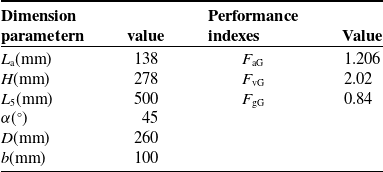
Without loss of generality, a set of dimensional parameters of the robot is given in Table I. Based on the planned trajectory, the inverse kinematics analysis is conducted. The obtained trajectory, along with the displacement, velocity, and acceleration of the driving joint over time, is shown in Figure 5.
Dimensional parameters of the parallel robot.

Table I. Long description
A table titled ’Dimensional parameters of the parallel robot’ with two columns and six rows. The columns are labeled ’Parameter’ and ’Numerical value/(m)’. The rows list the parameters and their corresponding numerical values. Row 1: Parameter, L3; Numerical value/(m), 0.12. Row 2: Parameter, L4; Numerical value/(m), 0.17. Row 3: Parameter, L5; Numerical value/(m), 0.065. Row 4: Parameter, L3; Numerical value/(m), 0.5. Row 5: Parameter, L5; Numerical value/(m), 0.556.
The operating states of the robot at different moments during the MSC-Adams simulation process.

From Figure 5(a) to Figure 5(d), it can be observed that the simulation curves are smooth, continuous, and free of abrupt changes. The displacement, velocity, and acceleration curves of the driving joints are successively differentiable, indicating that the planned rectangular trajectory has a reasonable motion law and coherent curves, enabling the robot to effectively accomplish the tasks of grasping and placing products in industrial production.
To validate the effectiveness of the aforementioned kinematic model, virtual motion simulation of the mechanism was conducted using the multi-body dynamics software MSC-Adams. Displacement data of the driving sliders were derived from the inverse kinematic model for a predefined rectangular trajectory of the end-effector and imported into MSC-Adams as input parameters for the active joints. Forward kinematic analysis was performed using MSC-Adams’ simulation solver, with the output process shown in Figure 6. The continuous and uninterrupted motion of the end-effector, along with the absence of interference between mechanism branches, confirms the rationality of the mechanism design.
4. Rigid body dynamics analysis
Before the rigid body dynamics modeling, friction and the energy loss caused by friction are neglected. In this paper, the refined and simplified rigid body dynamics models of the TGU-SV2 parallel robot are established, respectively. The system dynamics model of the TGU-SV2 parallel robot is derived based on the principle of virtual work, and the reliability of the dynamic model is validated by comparing the results of SolidWorks & Simscape co-simulation with the theoretical model.
4.1. Refined modeling for rigid body dynamics
4.1.1. Analysis of velocity and acceleration of each component
For convenience in conducting kinematic and dynamic analyses, as well as facilitating the design optimization of the parallel robot, it is divided into five modules from top to bottom: the fixed platform module, linear drive module, connecting frame module, passive arm module, and end-moving platform module. The linear drive module is responsible for providing the primary translational motion via its integrated actuation components, acting as the “power source” for the robot’s movement. The connecting frame module acts as a crucial intermediary structure, ensuring the coordinated transmission of motion and force between the linear drive units and the passive arms while maintaining geometric constraints. In the analysis, bolt-nut, small-sized, and lightweight components of each module are temporarily ignored, as these elements have minimal influence on the overall structural stiffness, motion characteristics, and dynamic responses of the robot system at the macro level. This simplification allows for a clearer focus on the core structural interactions and kinematic behaviors of the major modules, which is beneficial for establishing preliminary analytical models and conducting initial simulations to verify the robot’s basic performance, as depicted in Figure 7.
Analysis diagram of each module.

According to the kinematics analysis, in the linear drive module, the drive slider can only move relative to the guide groove direction of the guide rail, and its movement direction is
 ${\textit A}_{{\textit i}}{\textit C}_{{\textit i}}$
. According to Eq. (14), the centroid velocity of the driving slider is
 \begin{equation} \boldsymbol{v}_{\mathrm{s}\textit{i}}=\overset{.}{\mathrm{h}}_{{\textit i}}\,\boldsymbol{b}_{\textit{i}}=\boldsymbol{b}_{\textit{i}}\,\boldsymbol{J}_{\textit{i}}\boldsymbol{v} = \boldsymbol{J}_{\textit{i}1}\boldsymbol{v} \, \left(\textit{i}=1,2\right) \end{equation}
where
 $\boldsymbol{J}_{\textit{i}1}=\boldsymbol{b}_{\textit{i}}\,\boldsymbol{J}_{\textit{i}} , \boldsymbol{J}_{\textit{i}1}$
is the mapping matrix between the linear velocity
 $\boldsymbol{v}_{\mathrm{s}\textit{i}}$
of the driving slider and the output velocity
 $\boldsymbol{v}$
of the end-moving platform, and its matrix dimension is 3 × 3;
 $\boldsymbol{J}_{\textit{i}}$
is the i-th row of the system Jacobian matrix
 $\boldsymbol{J}$
.
Since the slider connecting frame is fixed with the driving slider of the linear driving module, the relative position between the slider connecting frame and the centroid of the driving slider remains unchanged, and the motion direction of the connecting frame is parallel to the direction
 ${\textit A}_{{\textit i}}{\textit C}_{{\textit i}}$
. According to the kinematics analysis, the overall centroid velocity of the connecting frame module is
 \begin{equation} \boldsymbol{v}_{\mathrm{h}\textit{i}}=\overset{.}{\mathrm{h}}_{{\textit i}}\,\boldsymbol{b}_{\textit{i}}=\boldsymbol{b}_{\textit{i}}\,\boldsymbol{J}_{\textit{i}}\boldsymbol{v} = \boldsymbol{J}_{\textit{i}1}\boldsymbol{v} \, \left(\textit{i}=1,2\right) \end{equation}
where
 $\boldsymbol{J}_{\textit{i}1}=\boldsymbol{b}_{\textit{i}}\,\boldsymbol{J}_{\textit{i}}, \boldsymbol{J}_{\textit{i}1}$
is also the mapping matrix between the linear velocity
 $\boldsymbol{v}_{\mathrm{h}\textit{i}}$
of the connecting frame module and the output velocity
 $\boldsymbol{v}$
of the end-moving platform, and its matrix dimension is 3 × 3.
The Hooke hinge fork seat in the passive arm branch module is symmetrically arranged about the centroid of the carbon fiber rod, and the centroid of the passive arm branch module coincides with the geometric center of the carbon fiber rod. According to the kinematic analysis, the passive arm module can not only rotate around the corresponding axis of the Hooke hinge but also move as a whole with the motion of the connecting frame. Additionally, the long rod of the passive arm is a homogeneous, equal-section rod.
The centroid velocity and angular velocity of the passive arm module can be expressed as:
 \begin{equation} \left\{\begin{aligned} &\boldsymbol{v}_{\mathrm{d}\textit{i}}=\dfrac{1}{2}\big(\boldsymbol{v}+\dot{\textit{h}}_{{\textit i}}\,\boldsymbol{b}_{{\textit i}}\big)=\dfrac{1}{2}\left(\boldsymbol{E}_{3}+\boldsymbol{b}_{{\textit i}}\,\boldsymbol{J}_{{\textit i}}\right)\boldsymbol{v}=\boldsymbol{J}_{{\textit i}2}\boldsymbol{v}\left({\textit i}=1,2\right)\\[4pt]&\boldsymbol{\omega}_{{\textit i}}=\dfrac{\left[\boldsymbol{w}_{{\textit i}}\times\right]\big(\boldsymbol{v}-\dot{\textit{h}}_{{\textit i}}\,\boldsymbol{b}_{{\textit i}}\big)}{{\textit L}_{5}}=\dfrac{\left[\boldsymbol{w}_{{\textit i}}\times\right]\left(\boldsymbol{E}_{3}-\boldsymbol{b}_{{\textit i}}\,\boldsymbol{J}_{{\textit i}}\right)}{{\textit L}_{5}}\boldsymbol{v}=\boldsymbol{J}_{\omega{\textit i}}\boldsymbol{v}\left({\textit i}=1,2\right) \end{aligned} \right.\end{equation}
where
 $\boldsymbol{J}_{{\textit i}2}$
is the mapping matrix between the centroid velocity
 $\boldsymbol{v}_{\mathrm{d}\textit{i}}$
of the passive arm and the end output
 $\boldsymbol{v}$
, and its expression is
 $\boldsymbol{J}_{{\textit i}2}=0.5(\boldsymbol{E}_{3}+\boldsymbol{b}_{\textit{i}}\,\boldsymbol{J}_{\textit{i}})$
, and its matrix dimension is 3 × 3;
 $\boldsymbol{J}_{{\unicode{x03C9}} {\textit i}}$
is the mapping matrix between the passive arm’s angular velocity
 $\boldsymbol{\omega }_{{\textit i}}$
and the end output
 $\boldsymbol{v}$
, and its expression is
 $\boldsymbol{J}_{{\unicode{x03C9}} {\textit i}}=[\boldsymbol{w}_{{\textit i}}\times ](\boldsymbol{E}_{3}-\boldsymbol{b}_{{\textit i}}\,\boldsymbol{J}_{{\textit i}})/{\textit L}_{5}$
, and its matrix dimension is 3 × 3. In the above equation,
 $\boldsymbol{E}_{3}$
is the third-order unit matrix, and
 $[\boldsymbol{w}_{{\textit i}}\times ]$
is the third-order antisymmetric matrix generated by
 $\boldsymbol{w}_{{\textit i}}$
.
According to the DOF analysis, the end-moving platform can only achieve two DOFs in the y and z directions, and there is no rotational DOF. The centroid velocity of the end-moving platform is
 \begin{align} \boldsymbol{v}=\left(\begin{array}{lll} 0 &\quad \overset{.}{\textit{y}} &\quad \overset{.}{\textit{z}} \end{array}\right)^{\mathrm{T}} \\[-25pt] \nonumber \end{align}
4.1.2. Acceleration analysis
According to Eq. (17), in the linear drive module, the centroid acceleration of the drive slider is
 \begin{equation} \boldsymbol{a}_{\mathrm{s}{\textit i}} = \overset{\mathit{.}\mathit{.}}{{\textit h}}_{{\textit i}}\,\boldsymbol{b}_{{\textit i}}\left({\textit i}=1,2\right) \end{equation}
where
 $\boldsymbol{a}_{\mathrm{s}\textit{i}}$
is the output acceleration of the reference point
 ${\textit P}$
of the end-0moving platform, and its matrix dimension is 3 × 1, and
 $\boldsymbol{b}_{{\textit i}}$
represents the unit direction vector of each drive slider.
Because the slider connecting frame is fixed with the driving slider, the analysis is similar to that for the velocity. The centroid acceleration of the connecting frame is
 \begin{equation} \boldsymbol{a}_{\mathrm{h}{\textit i}} = \overset{\mathit{.}\mathit{.}}{{\textit h}}_{{\textit i}}\,\boldsymbol{b}_{{\textit i}} \left({\textit i} = 1,2\right) \end{equation}
According to the kinematic analysis, the centroid acceleration and angular acceleration of the passive arm can be expressed as:
 \begin{equation} \left\{\begin{aligned}& \dot{\boldsymbol{\omega}}_{{\textit i}}= \dfrac{\left[\boldsymbol{w}_{{\textit i}}\times\right] \left(\boldsymbol{a}-\ddot{{\textit h}}_{{\textit i}}\,\boldsymbol{b}_{{\textit i}} -{\textit L}_{5}\left(\boldsymbol{\omega}_{{\textit i}}\times \left(\boldsymbol{\omega}_{{\textit i}}\times\boldsymbol{w}_{{\textit i}}\right)\right)\right)} {{\textit L}_{5}} \quad\left({\textit i}=1,2\right)\\[2pt]&\boldsymbol{a}_{\mathrm{d}{\textit i}}= \dfrac{1}{2}\left(\boldsymbol{a}+\ddot{{\textit h}}_{{\textit i}}\,\boldsymbol{b}_{{\textit i}}\right) \end{aligned} \right. \end{equation}
The centroid acceleration of the end-moving platform module is:
 \begin{align} \boldsymbol{a} = \left(\begin{array}{lll} 0 &\quad \overset{..}{\textit{y}} &\quad \overset{..}{\textit{z}} \end{array}\right)^{\mathrm{T}} \\[-25pt] \nonumber \end{align}
4.1.3. Force analysis of each component
The D’Alembert principle is applied to obtain the inertia force and inertia moment of each component, thus transforming the dynamic problem of the mechanism into a static balance problem for study.
The driving slider of the linear driving module moves relatively along the
 ${\textit A}_{{\textit i}}{\textit C}_{{\textit i}}$
direction, and the driving slider does not rotate. The force acting on the driving slider is mainly influenced by the inertia force and gravity, and there is no influence of the inertia moment. The expressions for the inertia force and gravity of the driving slider are given as:
 \begin{equation} \boldsymbol{F}_{\mathrm{s}\textit{i}}=-\textit{m}_{\mathrm{s}}\,\boldsymbol{a}_{\mathrm{s}{\textit i}}, \, \boldsymbol{G}_{\mathrm{s}{\textit i}}=\textit{m}_{\mathrm{s}}\,\boldsymbol{g}\left(\textit{i}=1,2\right) \end{equation}
where
 ${\textit m}_{\mathrm{s}}$
is the mass of the driving slider and
 $\boldsymbol{g}$
is the gravity acceleration vector; the matrix dimensions of
 $\boldsymbol{F}_{\mathrm{s}\textit{i}}$
and
 $\boldsymbol{G}_{\mathrm{s}{\textit i}}$
are both 3 × 1.
The connecting frame module is fixed with the driving slider, and it moves parallel to the
 ${\textit A}_{{\textit i}}{\textit C}_{{\textit i}}$
direction. The force acting on the connecting frame module is the same as that of the driving slider. The expressions for the inertia force and gravity of the connecting frame module are given as:
 \begin{equation} \boldsymbol{F}_{\mathrm{h}\textit{i}}=-\mathrm{m}_{\mathrm{h}}\,\boldsymbol{a}_{\mathrm{h}{\textit i}}, \, \boldsymbol{G}_{\mathrm{h}{\textit i}}=\mathrm{m}_{\mathrm{h}} \, \boldsymbol{g}\left(\textit{i}=1,2\right) \end{equation}
where
 ${\textit m}_{\mathrm{h}}$
is the mass of the connecting frame; the matrix dimensions of
 $\boldsymbol{F}_{\mathrm{h}\textit{i}}$
and
 $\boldsymbol{G}_{\mathrm{h}{\textit i}}$
are both 3 × 1.
The passive arm is influenced by inertia force, gravity, and inertia moment. The expressions for the inertia moment, inertia force, and gravity of the passive arm module are as follows:
 \begin{equation} \boldsymbol{M}_{\mathrm{d}i}=-\left(\boldsymbol{I}_{\mathrm{rod}}\,\overset{.}{\boldsymbol{\omega }}_{i}+\boldsymbol{\omega }_{i}\times \left(\boldsymbol{I}_{\mathrm{rod}}\boldsymbol{\omega }_{i}\right)\right), \, \boldsymbol{F}_{\mathrm{d}i}=-{\textit m}_{\mathrm{d}} \, \boldsymbol{a}_{\mathrm{d}i}, \boldsymbol{G}_{\mathrm{d}{\textit i}}={\textit m}_{\mathrm{d}}\boldsymbol{g}\left(i=1,2,3,4\right) \end{equation}
where
 $\boldsymbol{I}_{\mathrm{rod}}$
is the moment of inertia of the passive arm branch chain,
 $\mathrm{m}_{\mathrm{d}}$
is the mass of the passive arm branch chain; the matrix dimensions of
 $\boldsymbol{F}_{\mathrm{d}\textit{i}}$
and
 $\boldsymbol{G}_{\mathrm{d}{\textit i}}$
are both 3 × 1, while the matrix dimension of
 $\boldsymbol{M}_{\mathrm{d}i}$
is 3 × 3.
The end-moving platform module can only do two DOF translation in the
 $\mathrm{yoz}$
plane, without rotation. The moving platform is mainly affected by inertial force and gravity. The expressions of the inertial force and gravity on the moving platform are expressed as:
 \begin{equation} \boldsymbol{F}_{\mathrm{P}}=-\mathrm{m}_{\mathrm{P}} \, \boldsymbol{a},\boldsymbol{G}_{\mathrm{P}}=\mathrm{m}_{\mathrm{P}} \, \boldsymbol{g} \end{equation}
where
 ${\textit m}_{\mathrm{P}}$
is the mass of the connecting frame, and the matrix dimensions of
 $\boldsymbol{F}_{\mathrm{P}}$
and
 $\boldsymbol{G}_{\mathrm{P}}$
are both 3 × 1.
4.1.4. Establishment of the complete dynamics model of system
According to the principle of virtual power, the dynamic equilibrium equation of the robot is established, that is, the sum of the virtual power done by all forces of each component must be zero. Thus, we obtain:
 \begin{align} & \boldsymbol{f}^{\mathrm{T}}{\unicode{x0394}} \overset{\boldsymbol{.}}{\boldsymbol{h}}+\sum\limits_{i=1}^{2}\left({\boldsymbol{F}}_{\mathrm{s}{\textit i}}^{\mathrm{T}}{\unicode{x0394}} \boldsymbol{v}_{\mathrm{s}{\textit i}}+{\boldsymbol{G}}_{\mathrm{s}{\textit i}}^{\mathrm{T}}{\unicode{x0394}} \boldsymbol{v}_{\mathrm{s}{\textit i}}\right) +\sum\limits_{i=1}^{2}\left({\boldsymbol{F}}_{\mathrm{h}{\textit i}}^{\mathrm{T}}{\unicode{x0394}} \boldsymbol{v}_{\mathrm{h}{\textit i}}+{\boldsymbol{G}}_{\mathrm{h}{\textit i}}^{\mathrm{T}}{\unicode{x0394}} \boldsymbol{v}_{\mathrm{h}{\textit i}}\right)\nonumber \\&+\sum\limits_{i=1}^{4} \left({\boldsymbol{F}}_{\mathrm{d}i}^{\mathrm{T}}{\unicode{x0394}} \boldsymbol{v}_{\mathrm{d}{\textit i}}+{\boldsymbol{G}}_{\mathrm{d}i}^{\mathrm{T}}{\unicode{x0394}} \boldsymbol{v}_{\mathrm{d}{\textit i}}+{\boldsymbol{M}}_{\mathrm{d}i}^{\mathrm{T}}{\unicode{x0394}} \boldsymbol{\omega }_{{\textit i}}\right)+{\boldsymbol{F}}_{\mathrm{P}}^{\mathrm{T}}{\unicode{x0394}} \boldsymbol{v}+{\boldsymbol{G}}_{\mathrm{P}}^{\mathrm{T}}{\unicode{x0394}} \boldsymbol{v}=0 \end{align}
where
 $\boldsymbol{f}$
represents the driving force of each driving slider, and its matrix dimensions is 2 × 1, while
 ${\unicode{x0394}} \boldsymbol{v}_{\mathrm{s}{\textit i}} , {\unicode{x0394}} \boldsymbol{v}_{\mathrm{h}{\textit i}} , {\unicode{x0394}} \boldsymbol{v}_{\mathrm{d}{\textit i}}$
and
 ${\unicode{x0394}} \boldsymbol{v}$
denote the virtual velocity of the centroids of the driving slider, the connecting frame module, the passive arm branch and the moving platform, respectively. Additionally,
 ${\unicode{x0394}} \boldsymbol{\omega }_{{\textit i}}$
represents the virtual angular velocity of the passive arm branch. Based on the previous analysis of the velocities of each component, the corresponding expressions are as follows:
 ${\unicode{x0394}} \overset{\boldsymbol{.}}{\boldsymbol{h}}=\boldsymbol{J}{\unicode{x0394}} \boldsymbol{v} , {\unicode{x0394}} \boldsymbol{v}_{\mathrm{s}\textit{i}}=\boldsymbol{J}_{{\textit i}1}{\unicode{x0394}} \boldsymbol{v} , {\unicode{x0394}} \boldsymbol{v}_{\mathrm{h}{\textit i}}=\boldsymbol{J}_{{\textit i}1}{\unicode{x0394}} \boldsymbol{v} , {\unicode{x0394}} \boldsymbol{v}_{\mathrm{d}{\textit i}}=\boldsymbol{J}_{{\textit i}\mathrm{2}}{\unicode{x0394}} \boldsymbol{v} , {\unicode{x0394}} \boldsymbol{\omega }_{{\textit i}}=\boldsymbol{J}_{\mathit{\omega }{\textit i}}{\unicode{x0394}} \boldsymbol{v}$
.
Substituting Eq. (25) to Eq. (36) into Eq. (37), the refined rigid body dynamics model of the parallel robot can be expressed as follows:
 \begin{equation} \boldsymbol{f}=\left(\boldsymbol{J}^{+}\right)^{\mathrm{T}}\left(\begin{array}{l} -\displaystyle\sum\limits_{i=1}^{2}\left({\boldsymbol{J}}_{{\textit i}1}^{\mathrm{T}}\boldsymbol{F}_{\mathrm{s}{\textit i}}+{\boldsymbol{J}}_{{\textit i}1}^{\mathrm{T}}\boldsymbol{G}_{\mathrm{s}{\textit i}}\right)-\sum\limits_{i=1}^{2}\left({\boldsymbol{J}}_{{\textit i}1}^{\mathrm{T}}\boldsymbol{F}_{\mathrm{h}{\textit i}}+{\boldsymbol{J}}_{{\textit i}1}^{\mathrm{T}}\boldsymbol{G}_{\mathrm{h}{\textit i}}\right)\\[8pt] -\displaystyle\sum\limits_{i=1}^{4}\left({\boldsymbol{J}}_{{\textit i}2}^{\mathrm{T}}\boldsymbol{F}_{\mathrm{d}{\textit i}}+{\boldsymbol{J}}_{{\unicode{x03C9}} {\textit i}}^{\mathrm{T}}\boldsymbol{M}_{\mathrm{d}i}+{\boldsymbol{J}}_{{\textit i}2}^{\mathrm{T}}\boldsymbol{G}_{\mathrm{d}{\textit i}}\right)-\boldsymbol{F}_{\mathrm{P}}-\boldsymbol{G}_{\mathrm{P}} \end{array}\right) \end{equation}
where
 $\boldsymbol{J}^{+}$
denotes the generalized inverse of the Jacobian matrix
 $\boldsymbol{J}$
, and the matrix dimensions of
 $\boldsymbol{J}^{+}$
is 3 × 2. The derived model accounts for full rigid-body inertial effects, including centrifugal and Coriolis forces.
In order to facilitate subsequent numerical calculations and simulations, without loss of generality, the dimensional parameters of the parallel robot are shown in Table I, and the mass/inertia parameters are presented in Table II.
Mass/inertia parameters of the parallel robot.

Table II. Long description
A table with two columns and five rows. The first column is labeled ’parameter’ and the second column is labeled ’Numerical value’. The table lists the mass/inertia parameters of a parallel robot. Row 1: The passive arm relative to its spindle coordinate system, diag(1.51 x 10^-2, 3.50 x 10^-2, 1.50 x 10^-2). Row 2: m_si, 0.22 kg. Row 3: m_hi, 0.399 kg. Row 4: m_di, 0.2643 kg. Row 5: m_p, 0.213 kg.
4.1.5. Validation of multibody simulation model
To verify the correctness of the established refined dynamic model above, a virtual prototype of TGU-SV2 parallel robot is developed using the parameters from Tables I–II. The virtual prototype, established in SolidWorks, is imported into the Simulink environment via the Simscape Multibody plug-in for modular packaging. The simulation test model shown in Figure 8 is built, where the fixed platform, linear drive module, connecting frame module, passive arm module, and moving platform module are interconnected using the motion pair module, mirroring the joint connections in the physical prototype. The previously planned Gantry-style trajectory is used as an input signal to drive the moving platform.
Physical simulation model.

To verify the theoretical model, the simulation was implemented in MATLAB/Simscape. The solver type was selected as ode45 (Dormand-Prince) with a variable-step size to ensure numerical accuracy while solving for the driving forces. The total simulation time was set to 2 s to cover the complete motion trajectory.
The driving forces of the two driving joints are obtained through simulation tests and compared with the numerical calculation results derived from the refined dynamic model. An error analysis is conducted, as shown in Figure 9. As depicted in the figure, the maximum driving force is 56.50 N, and the maximum driving force error is approximately 0.98 N. The main causes of the error between theoretical and simulation values are measurement errors in inertial parameters and mass. The above analysis shows that the theoretical calculation results are in high consistency with the multibody simulation results. The comparative results verify the high-precision characteristics of the derived dynamic model, providing a solid theoretical foundation for subsequent optimization design, control strategy research, parameter identification, and other works.
Comparison on driving force of actuate joints and errors. (a) The driving force of actuating joint 1. (b) The driving force of actuating joint 2. (c) The driving force error of actuating joints.

4.2. Simplified modeling for rigid body dynamics
The long rod of the passive arm in the proposed parallel mechanism is made of light carbon fiber, which offers advantages such as low weight and high strength. As a result, its mass and moment of inertia are relatively small and can be ignored. Using the equivalent principle of statics, the mass of the four driven branches of the mechanism is distributed between the connecting frame and the moving platform in a 1:2 ratio. This approach simplifies the modeling process and reduces computational complexity. By excluding energy loss due to friction at each joint, the rigid body dynamics model of the TGU-SV2 parallel robot is analyzed using the virtual work principle. The establishment of this simplified model ensures both accuracy and effectiveness, while making the model more concise. This reduction in complexity facilitates future performance analysis, dimension optimization.
The simplified rigid body dynamics model of TGU-SV2 parallel robot can be expressed as:
 \begin{equation} \boldsymbol{F}^{\mathrm{T}}{\unicode{x0394}} \overset{\boldsymbol{.}}{\boldsymbol{h}} + \sum\limits_{{\textit i} = 1}^{2}\left({\boldsymbol{F}}_{\mathrm{s}{\textit i}}^{\mathrm{T}}{\unicode{x0394}} \boldsymbol{v}_{\mathrm{s}{\textit i}} + {\boldsymbol{G}}_{\mathrm{s}{\textit i}}^{\mathrm{T}}{\unicode{x0394}} \boldsymbol{v}_{\mathrm{s}{\textit i}}\right) + \sum\limits_{{\textit i} = 1}^{2}\left({\boldsymbol{F}}_{\mathrm{eq}{\textit i}}^{\mathrm{T}}{\unicode{x0394}} \boldsymbol{v}_{\mathrm{h}{\textit i}}+{\boldsymbol{G}}_{\mathrm{eq}{\textit i}}^{\mathrm{T}}{\unicode{x0394}} \boldsymbol{v}_{\mathrm{h}{\textit i}}\right)+{\boldsymbol{F}}_{\mathrm{Pa}}^{\mathrm{T}}{\unicode{x0394}} \boldsymbol{v} + {\boldsymbol{G}}_{\mathrm{Pa}}^{\mathrm{T}}{\unicode{x0394}} \boldsymbol{v}=0 \end{equation}
where
 $\boldsymbol{F}$
represents the driving force of each driving slider and its matrix dimensions is 2 × 1,
 $\boldsymbol{F}_{\mathrm{s}{\textit i}}$
denotes the inertial force of the driving slider, and
 $\boldsymbol{G}_{\mathrm{s}{\textit i}}$
is the gravity acting on the driving slider. Similarly,
 $\boldsymbol{F}_{\mathrm{eq}{\textit i}}$
and
 $\boldsymbol{G}_{\mathrm{eq}{\textit i}}$
correspond to the inertial force and gravity of the equivalent connecting frame, respectively, while
 $\boldsymbol{F}_{\mathrm{Pa}}$
and
 $\boldsymbol{G}_{\mathrm{Pa}}$
represent the inertial force and gravity of the equivalent moving platform. Additionally,
 ${\unicode{x0394}} \overset{\boldsymbol{.}}{\boldsymbol{h}}$
is the virtual displacement of the driving slider, which is equal to the virtual displacement of the equivalent connecting frame, and
 ${\unicode{x0394}} \boldsymbol{r}$
is the virtual displacement of the equivalent moving platform.
According to the above analysis of the velocity and acceleration of each component, the following relationship can be obtained:
 \begin{equation} {\unicode{x0394}} \overset{\boldsymbol{.}}{\boldsymbol{h}} = \boldsymbol{J}{\unicode{x0394}} \boldsymbol{v},{\unicode{x0394}} \boldsymbol{v}_{\mathrm{s}\textit{i}}=\boldsymbol{J}_{{\textit i}1}{\unicode{x0394}} \boldsymbol{v},{\unicode{x0394}} \boldsymbol{v}_{\mathrm{h}\textit{i}}=\boldsymbol{J}_{{\textit i}1}{\unicode{x0394}} \boldsymbol{v} \left({\textit i} = \mathrm{1, 2}\right) \end{equation}
Substituting Eq. (40) into Eq. (39), the simplified rigid body dynamics model of the TGU-SV2 parallel robot can be obtained as follows:
 \begin{equation} \boldsymbol{F}=\left(\boldsymbol{J}^{+}\right)^{\mathrm{T}}\left(-\sum\limits_{{\textit i} = 1}^{2}\left({\boldsymbol{F}}_{\mathrm{s}{\textit i}}^{\mathrm{T}}\boldsymbol{J}_{{\textit i}1} + {\boldsymbol{G}}_{\mathrm{s}{\textit i}}^{\mathrm{T}}\boldsymbol{J}_{{\textit i}1}\right)-\sum\limits_{{\textit i} = 1}^{2}\left({\boldsymbol{F}}_{\mathrm{eq}{\textit i}}^{\mathrm{T}}\boldsymbol{J}_{{\textit i}1}+{\boldsymbol{G}}_{\mathrm{eq}{\textit i}}^{\mathrm{T}}\boldsymbol{J}_{{\textit i}1}\right)-{\boldsymbol{F}}_{\mathrm{Pa}}^{\mathrm{T}}-{\boldsymbol{G}}_{\mathrm{Pa}}^{\mathrm{T}}\right)^{\mathrm{T}} \end{equation}
Eq. (41) is further organized into a normalized expression, resulting in the following form:
 \begin{equation} \boldsymbol{F} = \boldsymbol{M}\left(\boldsymbol{r}\right)\boldsymbol{a}+\boldsymbol{C}\left(\boldsymbol{r},\overset{\boldsymbol{.}}{\boldsymbol{r}}\right)\boldsymbol{v}+\boldsymbol{G}\left(\boldsymbol{r}\right) \end{equation}
where
 $\boldsymbol{M}(\boldsymbol{r})$
denotes the inertial force matrix,
 $\boldsymbol{C}(\boldsymbol{r},\overset{\boldsymbol{.}}{\boldsymbol{r}})$
represents the centrifugal/coriolis force matrix, and
 $\boldsymbol{G}(\boldsymbol{r})$
stands for the gravitational force matrix.
 \begin{equation} \left\{ \begin{aligned} &\boldsymbol{M}\left(\boldsymbol{r}\right)= \left(\boldsymbol{J}^{+}\right)^{\mathrm{T}} \left(\left({\textit m}_{\mathrm{s}}+{\textit m}_{\mathrm{eq}}\right) \sum_{{\textit i}=1}^{2}\boldsymbol{J}_{{\textit i}}^{\mathrm{T}}\boldsymbol{J}_{{\textit i}} +{\textit m}_{\mathrm{Pa}}\right)\\& \boldsymbol{C}\left(\boldsymbol{r},\dot{\boldsymbol{r}}\right)= \left(\boldsymbol{J}^{+}\right)^{\mathrm{T}} \left(\left({\textit m}_{\mathrm{s}}+{\textit m}_{\mathrm{eq}}\right) \sum_{{\textit i}=1}^{2}\boldsymbol{J}_{{\textit i}}^{\mathrm{T}} \boldsymbol{v}^{\mathrm{T}}\boldsymbol{H}_{{\textit i}}\right)\\ &\boldsymbol{G}\left(\boldsymbol{r}\right)= -\left(\boldsymbol{J}^{+}\right)^{\mathrm{T}} \left(\left({\textit m}_{\mathrm{s}}+{\textit m}_{\mathrm{eq}}\right) \sum_{{\textit i}=1}^{2}\boldsymbol{J}_{{\textit i}}^{\mathrm{T}} \boldsymbol{b}_{{\textit i}}^{\mathrm{T}}+{\textit m}_{\mathrm{Pa}}\right)\boldsymbol{g} \end{aligned} \right. \end{equation}
where
 ${\textit m}_{\mathrm{eq}}$
is the mass of the equivalent connecting frame, and
 ${\textit m}_{\mathrm{Pa}}$
is the mass matrix of the equivalent moving platform.
To verify the effectiveness of the simplified dynamic model, the previously used test trajectory is employed for an inverse dynamic numerical simulation. The results from the simplified dynamic model are compared with those obtained from the simulation test, and an error analysis is performed, as shown in Figure 10. By examining the error curves of both models, it is observed that the maximum driving force error does not exceed 2.5 N.
Comparison on driving force of actuate joints and errors. (a) The driving force of actuating joint 1. (b) The driving force of actuating joint 2. (c) The driving force error of actuating joints.

The above analysis demonstrates that the simplified dynamic model, based on the proposed simplification principle, offers good solution accuracy. Additionally, a comparison between the two dynamic models reveals that the more accurate model closely matches the simulation curve, while the simplified model shows a slightly larger deviation. However, the simplified model excels in terms of mathematical expression and calculation procedure, offering high solution efficiency. This makes it an ideal choice for subsequent dynamic performance analysis and indicator extraction, as it strikes a balance between computational simplicity and accuracy.
4.3. Verification of the impact of model simplification on accuracy
To verify the influence of model simplification on power accuracy, the power characteristics (including energy consumption and power errors) between the accurate dynamic model and the simplified dynamic model are compared. The results for the system’s power consumption (reflecting overall energy performance) and the power errors of actuating joints 1 and 2 are as shown in Figure 11.
Comparison of power and errors between the accurate model and the simplified mode. (a) The power of actuating joint 1. (b) The power of actuating joint 2. (c) Power error between the accurate model and the simplified model.

From the power consumption curves (the first two subfigures), the variation trends of power for the accurate model and the simplified model are highly consistent. Although there are slight differences in peak values (e.g., the accurate model reaches approximately 65.0678 W while the simplified model shows around 65.044 W at certain moments, and similar consistency is observed in the second power consumption curve), the overall fluctuation patterns match well.
For the power errors (the third subfigure), the power errors of actuating joints 1 and 2 remain within a relatively narrow range throughout the motion process. The peak power error does not exceed 5 W, and error values fluctuate within ±4.219 W. Considering the typical power magnitude in practical parallel robot systems (often ranging from dozens to hundreds of watts), such error levels indicate that simplification has a limited impact on the model’s power accuracy.
Therefore, the simplified dynamic model can sufficiently capture the key power characteristics of the robot while reducing computational complexity, meeting the requirements for engineering analysis and application in energy performance evaluation.
5. Dynamic dimensional synthesis
5.1. Workspace and dimensional design variables
When a set of dimensional parameters of the robot are given, such as the length
 ${\textit L}_{5}$
of the passive arm, the horizontal distance
 ${\textit L}_{\mathrm{a}}$
of the static platform and the stroke of the guide rail prismatic pair, as shown in Figure 12, the reachable workspace
 ${\textit W}$
of the reference point
 ${\textit P}$
of the moving platform can be described geometrically. Specifically, when the displacement of the slider reaches its limit position, the passive arm revolves around the axis of the equivalent rotating pair of the connecting frame, tracing a circle with its length as the radius. This motion generates a geometric closed body composed of the common area enveloped by the four circles. This defines the boundary of the reachable workspace of the moving platform.
Schematic diagram of the scale and task workspace of the parallel robot.

According to the actual work requirements, it is typically sufficient for the end effector to complete the established task within a defined time interval. A maximum rectangular space can be defined as the task workspace
 ${\textit W}_{\mathrm{t}}$
of the robot. The task workspace is defined as follows: the width of the task workspace is defined as parameter
 ${\textit D}$
, the height as parameter
 ${\textit b}$
, and the distance between the upper boundary of the task workspace and the origin
 ${\textit O}$
of the static coordinate system of the robot is defined as parameter
 ${\textit H}$
. These parameters define the spatial limits within which the robot must operate to achieve the desired task.
Therefore, the dynamic dimensional synthesis of the robot can be expressed as follows: given the task workspace dimensions, considering the overall performance of the robot within the specified workspace, and incorporating the relevant performance constraints, a set of dimension parameters
 ${\textit L}_{\mathrm{a}} , \hat{{\textit L}}_{5}$
, and
 ${\textit H}$
along with the structural angle
 $\alpha$
are synthesized to optimize the robot’s global performance in the task workspace, where
 $\hat{{\textit L}}_{5}$
denotes the equivalent length of the spatial structure of the passive arm.
5.2. Evaluation index of dynamic performance
Parallel robots for high-speed grasping and releasing often need to start, accelerate, decelerate, and stop frequently in the workspace and maintain high speed and acceleration in each motion state, and instantaneous transformation should be completed between each operation state. The above operation requires that the end-effector of the parallel robot with high-speed grasping and releasing operation has a very high running speed in a given workspace and maintains a very high positioning accuracy during high-speed operation.
In summary, the following dynamic performance evaluation indices can be defined based on the rigid body dynamics discussed above ref. [Reference Peng, Zhu and Niu38]. These indices can then be used to construct the objective function for dimensional synthesis. By considering the relevant kinematic performance constraints of the parallel robot, a set of dimension parameters can be synthesized to optimize the global performance of the parallel robot within the given task workspace.
(1) Inertia force performance evaluation index
It can be seen from Eq. (42) that the contribution of the inertia term of the parallel robot to the uniaxial driving force can be expressed as:
 \begin{equation} {\textit F}_{\mathrm{a}\mathit{,}{\textit i}}=\boldsymbol{M}_{{\textit i}}\boldsymbol{a}({\textit i} = 1,2) \end{equation}
where
 $\boldsymbol{M}_{{\textit i}}$
denotes the row vector of the i-th row of
 $\boldsymbol{M}$
.
According to the principle of matrix singular value decomposition (SVD), to achieve unit acceleration (
 $||\boldsymbol{a}|| = 1$
) at the reference point
 ${\textit P}$
of the moving platform in a specific configuration, the maximum value of the required joint driving force can be expressed as:
 \begin{equation} {\textit F}_{\mathrm{a}{\textit i}\mathit{,}\max }=\mathit{\sigma }_{\text{amax}\mathit{,}{\textit i}}\left(\boldsymbol{M}_{{\textit i}}\right)=\sqrt{\boldsymbol{M}_{{\textit i}}{\boldsymbol{M}}_{{\textit i}}^{\mathrm{T}}} \end{equation}
Combined with the inverse rigid body dynamics of the parallel robot and the above formula, it can be observed that the maximum joint driving force required to achieve unit acceleration (
 $||\boldsymbol{a}||=1$
) at the reference point
 ${\textit P}$
on the moving platform is a function of the robot’s dimension parameters, inertia parameters, and configuration parameters. Therefore, minimizing the global maximum value of
 $\max _{{\textit i}=1,2}(\sigma _{\text{amax}\mathit{,}{\textit i}}(\boldsymbol{M}_{{\textit i}}))$
is considered one of the dynamic performance optimization objectives. This can be expressed as:
 \begin{equation} \min _{\boldsymbol{x}}\Big({\textit F}_{\mathrm{aG}}=\max _{\boldsymbol{r}\in \mathrm{W}_{\mathrm{t}}}\Big(\max _{{\textit i}=1,2}\left(\sigma _{\text{amax}\mathit{,}{\textit i}}\left(\boldsymbol{M}_{{\textit i}}\right)\right)\Big)\Big) \end{equation}
where
 $\boldsymbol{r}$
is the generalized coordinate position vector of the moving platform reference point
 ${\textit P}$
, and
 $\boldsymbol{x} = ({\textit L}_{\mathrm{a}},{\textit L}_{5},{\textit H},\alpha )$
denotes the set of design variables.
(2) Centrifugal force / Coriolis force performance evaluation index
It can be seen from Eq. (42) that the contribution of the velocity term of the parallel robot to the uniaxial driving force can be expressed as:
 \begin{equation} {\textit F}_{\mathrm{v}\mathit{,}{\textit i}}=\left({\textit m}_{\mathrm{eq}}+{\textit m}_{\mathrm{s}}\right)\boldsymbol{v}^{\mathrm{T}}\boldsymbol{H}_{{\textit i}}\boldsymbol{v}\,({\textit i} = 1,2) \end{equation}
where
 $\boldsymbol{H}_{{\textit i}}$
is the Hessian matrix.
According to the principle of matrix SVD, given
 $||\boldsymbol{v}||=1$
, the maximum value of
 $\boldsymbol{H}_{{\textit i}}$
can be expressed as the maximum singular value of the velocity term matrix, and
 $\boldsymbol{H}_{{\textit i}}$
is a function of the dimension parameters, inertial parameters and configuration parameters of the parallel robot. When a singularity occurs in the parallel robot, the output force of the velocity term will tend to infinity. Therefore, minimizing the global maximum value of the maximum singular value of matrix
 $\boldsymbol{H}_{{\textit i}}$
is taken as the second dynamic performance optimization objective, which is expressed as:
 \begin{equation} \min _{\boldsymbol{x}}\Big({\textit F}_{\mathrm{vG}}=\max _{\boldsymbol{r}\in \mathrm{W}_{\mathrm{t}}}\Big(\max _{{\textit i}=1,2}\left(\sigma _{\text{vmax}\mathit{,}{\textit i}}\left(\boldsymbol{H}_{{\textit i}}\right)\right)\Big)\Big) \end{equation}
(3) Gravity performance evaluation index
It can be seen from Eq. (42) that the contribution of the gravity term of the parallel robot to the uniaxial driving force can be expressed as:
 \begin{equation} {\textit F}_{\mathrm{g},{\textit i}} = \boldsymbol{Z}_{{\textit i}}\boldsymbol{g} = {\textit g}{\textit Z}_{{\textit i}3}({\textit i} = 1,2) \end{equation}
where
 $\boldsymbol{Z}_{{\textit i}}$
is the i-th row vector of the
 $\boldsymbol{Z}$
matrix, and
 ${\textit Z}_{{\textit i}3}$
represents the third element of
 $\boldsymbol{Z}$
. Therefore, the maximum value of
 $\boldsymbol{F}_{\mathrm{g},{\textit i}}/\mathrm{g}$
corresponds to the maximum value of
 $| {\textit Z}_{{\textit i}3}|$
, which reflects the influence of the gravity term on the driving force. Consequently, minimizing the global maximum value of
 $| {\textit Z}_{{\textit i}3}|$
is taken as the third dynamic performance optimization objective, that is,
 \begin{align} \min _{\boldsymbol{x}}\Big({\textit F}_{\mathrm{gG}}=\max _{\boldsymbol{r}\in \mathrm{W}_{\mathrm{t}}}\Big(\max _{{\textit i}=1,2}\left(\left| {\textit Z}_{{\textit i}3}\right| \right)\Big)\Big) \\[-20pt] \nonumber \end{align}
5.3. Constraint conditions
(1) Dimension constraint
The parallel robot is designed to install the linear drive modules on both sides of the static platform to ensure sufficient installation space. The parallel robot utilizes a passive arm to establish a connection between the moving platform and the frame while facilitating smooth assembly. To achieve this, the following conditions should be satisfied.
 \begin{equation} {\textit L}_{\text{amin}}\leq {\textit L}_{\mathrm{a}}\leq {\textit L}_{\text{amax}} \end{equation}
The parallel robot is actuated by a linear drive module, with the length of the screw having a direct impact on the overall structure and performance of the system. Therefore, to ensure optimal performance, the distance from the boundary to a point within the task workspace should satisfy the following constraints:
 \begin{equation} {\textit H}_{\min }\leq {\textit H}\leq {\textit H}_{\max } \end{equation}
The passive arm also plays a critical role in determining the overall stiffness and assembly conditions of the parallel robot. Therefore, the length of the passive arm should adhere to the following conditions.
 \begin{equation} \hat{{\textit L}}_{{5}{\min} }\leq \hat{{\textit L}}_{5}\leq \hat{{\textit L}}_{{5}{\max} } \end{equation}
Second, based on the geometric relationship and considering the two configurations of the branched chain shown in Figure 13 as an example, when the reference point P of the mechanism’s end effector moves to the lower edge position on one side of the workspace, the connecting frame and follower arm of the planar branch need to be sufficiently long to ensure that this position can be reached.
 \begin{equation} \sqrt{\left({\textit h}_{{2}{\min} }\sin \alpha +{\textit H}\mathit{+}{\textit h}\right)^{2}+\big({\textit h}_{{2}{\min} }\cos \alpha \mathit{+}{\textit D}/2+\big({\textit L}_{\mathrm{a}}-\hat{{\textit L}}_{6}\big)\big)^{2}}-{\textit L}_{\mathrm{c}}-\hat{{\textit L}}_{5}\lt0 \end{equation}
Two extreme positions of the parallel robot.

Additionally, when the reference point p of the robot’s end effector moves to the upper edge position of the workspace, it should approximately satisfy the following relationship.
 \begin{equation} \left\{ \begin{aligned} &\hat{{\textit L}}_{5}-{\textit h}_{{1}{\max}}\sin\alpha-{\textit H}+{\textit L}_{\mathrm{c}} \lt 0\\[3pt] &{\textit D}/2+\hat{{\textit L}}_{6}-{\textit L}_{\mathrm{a}}-{\textit h}_{{1}{\max}}\cos\alpha\lt0 \end{aligned} \right. \end{equation}
Considering the actual workspace and floor area of the parallel robot, the stroke of the slider can be determined by selecting an appropriate guide rail stroke that accommodates the required range of motion while optimizing the spatial constraints of the system.
 \begin{align} {\textit h}_{\max }\leq 0.365{\mathrm{m}} \end{align}
(2) Motion performance constraints
The kinematic performance of the parallel robot, which is designed to achieve high-speed grasping and releasing operations, is primarily influenced by factors such as speed, accuracy, stiffness, and load-bearing capacity. These aspects must be carefully considered during the design process to ensure optimal performance and reliability.
 ${\unicode{x2460}}$
Speed performance constraint
According to the kinematic analysis, the following results can be obtained:
 \begin{equation} \boldsymbol{v} = {\boldsymbol{J}}_{\mathrm{r}}^{-1}\overset{\boldsymbol{.}}{\boldsymbol{h}} \end{equation}
where
 $\boldsymbol{J}_{\mathrm{r}}$
represents the matrix composed of the second and third columns of the Jacobian matrix. Considering the actual configuration of the parallel robot,
 $\boldsymbol{J}_{\mathrm{r}}$
can be used to represent the actual Jacobian matrix of the parallel robot.
 ${\boldsymbol{J}}_{\mathrm{r}}^{-1}$
denotes the inverse matrix of
 $\boldsymbol{J}_{\mathrm{r}}$
.
According to the principle of matrix SVD, under the condition of
 $||\overset{\boldsymbol{.}}{\boldsymbol{h}}||=1$
, in order to ensure the higher speed characteristics of the parallel robot, the global minimum value of the singular values of
 ${\boldsymbol{J}}_{\mathrm{r}}^{-1}$
should be maximized. Given that
 $\sigma _{\min }({\boldsymbol{J}}_{\mathrm{r}}^{-1})=1/\sigma _{\max }(\boldsymbol{J}_{\mathrm{r}})$
represents the smallest singular value of the Jacobian matrix, it follows that:
 \begin{equation} \max _{\boldsymbol{x}}\Big(\min _{\boldsymbol{r}\in \mathrm{W}_{\mathrm{t}}}\left(\sigma _{\min }\left({\boldsymbol{J}}_{\mathrm{r}}^{-1}\right)\right)\Big)\Leftrightarrow \min _{\boldsymbol{x}}\Big(\max _{\boldsymbol{r}\in \mathrm{W}_{\mathrm{t}}}\left(\sigma _{\max }\left(\boldsymbol{J}_{\mathrm{r}}\right)\right)\Big) \end{equation}
To ensure that the speed of the moving platform is not less than a given value within the task workspace, the following performance constraints are established:
 \begin{equation} \max _{\boldsymbol{r}\in \mathrm{W}_{\mathrm{t}}}\left(\sigma _{\max }\left(\boldsymbol{J}_{\mathrm{r}}\right)\right)\leq \left[{\textit A}_{\mathrm{u}}\right] \end{equation}
where
 $[{\textit A}_{\mathrm{u}}]$
represents the upper bound of the global maximum singular value of
 $\boldsymbol{J}_{\mathrm{r}}$
. This bound ensures that the parallel robot operates within the desired velocity limits while maintaining its performance characteristics.
 ${\unicode{x2461}}$
Precision performance constraints
The mapping relationship between the pose error of the moving platform and the driving input error can be described using the Jacobian matrix of the parallel robot. Specifically, the pose error
 $\Delta \boldsymbol{r}$
of the moving platform is related to the driving input error
 $\Delta \boldsymbol{h}$
through the Jacobian matrix
 $\boldsymbol{J}_{\mathrm{r}}$
as follows:
 \begin{equation} \Delta \boldsymbol{r} = {\boldsymbol{J}}_{\mathrm{r}}^{-1}\Delta \boldsymbol{h} \end{equation}
Under the condition of
 $||\overset{\boldsymbol{.}}{\boldsymbol{h}}||=1$
, in order to ensure the high pose accuracy of the parallel robot, it is necessary to make:
 \begin{equation} \min _{\boldsymbol{x}}\Big(\max _{\boldsymbol{r}\in \mathrm{W}_{\mathrm{t}}}\left(\sigma _{\max }\left({\boldsymbol{J}}_{\mathrm{r}}^{-1}\right)\right)\Big)\Leftrightarrow \max _{\boldsymbol{x}}\Big(\min _{\boldsymbol{r}\in \mathrm{W}_{\mathrm{t}}}\left(\sigma _{\min }\left(\boldsymbol{J}_{\mathrm{r}}\right)\right)\Big) \end{equation}
In order to ensure that the pose error of the moving platform in the task workspace is not greater than the given value, the following performance constraints can be constructed:
 \begin{equation} \min _{\boldsymbol{r}\in \mathrm{W}_{\mathrm{t}}}\left(\sigma _{\min }\left(\boldsymbol{J}_{\mathrm{r}}\right)\right)\geq \left[{\textit A}_{\mathrm{d}}\right] \end{equation}
where
 $[{\textit A}_{\mathrm{d}}]$
represents the lower bound of the global minimum singular value of
 $\boldsymbol{J}_{\mathrm{r}}$
.
 ${\unicode{x2462}}$
Stiffness performance constraints
Assuming that the equivalent stiffness of the driving joint is a constant
 ${\textit k}_{{\textit i}}$
in the branch
 ${\textit i}$
, then the total stiffness of the parallel robot can be expressed as:
 \begin{equation} \boldsymbol{F}_{\mathrm{a}}=\mathrm{diag}({\textit k}_{{\textit i}})\Delta \boldsymbol{h} \end{equation}
If the deformation of the reference point
 ${\textit P}$
of the moving platform caused by the external force
 $\boldsymbol{F}_{\mathrm{P}}$
is
 $\Delta \boldsymbol{r}_{\mathrm{P}}$
, then the relationship between the deformation and the external force can be expressed as:
 \begin{equation} \boldsymbol{F}_{\mathrm{P}}=\boldsymbol{K}\Delta \boldsymbol{r}_{\mathrm{P}} \end{equation}
where
 $\boldsymbol{K} = {\boldsymbol{J}}_{\mathrm{r}}^{\mathrm{T}}\mathrm{diag}({\textit k}_{{\textit i}})\boldsymbol{J}_{\mathrm{r}}$
represents the driving stiffness matrix of the system, and
 ${\textit k}_{{\textit i}}=1$
is a given condition. Under the condition
 $||\Delta \boldsymbol{r}_{\mathrm{P}}||=1$
, which corresponds to the unit deformation of the moving platform, the global minimum of the minimum eigenvalue of matrix
 ${\boldsymbol{J}}_{\mathrm{r}}^{\mathrm{T}}\boldsymbol{J}_{\mathrm{r}}$
should be maximized. This optimization can be expressed as:
 \begin{equation} \min _{\boldsymbol{x}}\Big(\min _{\boldsymbol{r}\in \mathrm{W}_{\mathrm{t}}}\left(\lambda _{\min }\left({\boldsymbol{J}}_{\mathrm{r}}^{\mathrm{T}}\boldsymbol{J}_{\mathrm{r}}\right)\right)\Big) \end{equation}
It can be observed that
 $\lambda _{\min }({\boldsymbol{J}}_{\mathrm{r}}^{\mathrm{T}}\boldsymbol{J}_{\mathrm{r}})={\sigma }_{\min }^{2}(\boldsymbol{J}_{\mathrm{r}})$
; thus, the aforementioned equation is equivalent to:
 \begin{equation} \max _{\boldsymbol{x}}\Big(\min _{\boldsymbol{r}\in \mathrm{W}_{\mathrm{t}}}\left(\sigma _{\min }\left(\boldsymbol{J}_{\mathrm{r}}\right)\right)\Big) \end{equation}
In order to ensure the stiffness performance of the parallel robot within the task workspace, constraints consistent with the accuracy performance constraints can be constructed.
 ${\unicode{x2463}}$
Performance constraints of bearing capacity
The relationship between the virtual displacement
 $\Delta \boldsymbol{r}_{\mathrm{p}}$
of the moving platform and the virtual displacement
 $\Delta \boldsymbol{h}$
of the driving slider can be obtained by applying the principle of virtual displacement. This relationship is given by:
 \begin{equation} {\boldsymbol{F}}_{\mathrm{a}}^{\mathrm{T}}\Delta \boldsymbol{h}={\boldsymbol{F}}_{\mathrm{P}}^{\mathrm{T}}\Delta \boldsymbol{r}_{\mathrm{P}} \end{equation}
where
 $\boldsymbol{F}_{\mathrm{a}}$
is the driving force applied to the slider, and
 $\boldsymbol{F}_{\mathrm{P}}$
is the bearing capacity on the moving platform.
According to the kinematic analysis,
 $\Delta \boldsymbol{r}_{\mathrm{P}}$
(the virtual displacement of the moving platform) and
 $\Delta \boldsymbol{h}$
(the virtual displacement of the driving slider) satisfy the following mapping relationship:
 \begin{equation} \Delta \boldsymbol{h} = \boldsymbol{J}_{\mathrm{r}}\Delta \boldsymbol{r}_{\mathrm{P}} \end{equation}
Combining Eqs. (67) and (68), we can obtain the following:
 \begin{equation} \boldsymbol{F}_{\mathrm{P}}={\boldsymbol{J}}_{\mathrm{r}}^{\mathrm{T}}\boldsymbol{F}_{\mathrm{a}} \end{equation}
Therefore, according to the principle of matrix SVD, under the condition that the slider driving force is the unit driving force
 $||\boldsymbol{F}_{\mathrm{a}}||=1$
, in order to ensure that the moving platform has better theoretical bearing capacity, the minimum singular value of
 $\boldsymbol{J}_{\mathrm{r}}$
should be maximized, that is,
 \begin{equation} \max _{\boldsymbol{x}}\Big(\min _{\boldsymbol{r}\in \mathrm{W}_{\mathrm{t}}}\Big(\sigma _{\min }\left(\boldsymbol{J}_{\mathrm{r}}\right)\Big)\Big) \end{equation}
Therefore, in order to ensure the global carrying capacity of the moving platform in the task space, constraints consistent with the accuracy performance constraints can be constructed. Considering the performance constraints of speed, accuracy, stiffness, and bearing capacity, it is found that the mapping characteristics of accuracy, stiffness, and bearing capacity are similar, while the speed constraints are contradictory to them. Therefore, the performance constraints can be comprehensively weighted, and the appropriate
 $[{\textit A}_{\mathrm{u}}]$
and
 $[{\textit A}_{\mathrm{d}}]$
values can be selected to make the performance and dimensions of the parallel robot more reasonable in the task workspace.
By doing so, both the bearing capacity and stiffness of the parallel robot in the task workspace can be guaranteed, while reducing motion errors. This balanced approach ensures that the parallel robot operates optimally in terms of speed, accuracy, stiffness, and bearing capacity, maintaining high precision and performance throughout its range of operation.
(3) Construction of dynamic dimensional synthesis model
Based on the above-defined dimensional parameters, dynamic performance indices, and various constraints, the dynamic dimensional optimization of parallel robot studied in this paper can be summarized as the following constrained multiobjective optimization problem:
 \begin{equation} \begin{array}{l} \min \left\{\begin{array}{lll} {\textit F}_{\mathrm{aG}} & \ \ {\textit F}_{\mathrm{vG}} & \ \ {\textit F}_{\mathrm{gG}} \end{array}\right\}\\[5pt] \mathrm{s}.\mathrm{t}.\begin{cases} {\textit L}_{\text{amin}}\leq {\textit L}_{\mathrm{a}}\leq {\textit L}_{\text{amax}}\\[5pt] {\textit H}_{\min }\leq {\textit H}\leq {\textit H}_{\max }\\[5pt] \hat{{\textit L}}_{{5}{\min} }\leq \hat{{\textit L}}_{5}\leq \hat{{\textit L}}_{{5}{\max} }\\[5pt] {\textit h}_{\max }\leq 0.365\mathrm{m}\\[5pt] \sqrt{\left({\textit h}_{{2}{\min} }\sin \alpha +{\textit H}\mathit{+}{\textit h}\right)^{2}+\big({\textit h}_{{2}{\min} }\cos \alpha \mathit{+}{\textit D}/2+\big({\textit L}_{\mathrm{a}}-\hat{{\textit L}}_{6}\big)\big)^{2}}-{\textit L}_{\mathrm{c}}-\hat{{\textit L}}_{5}\lt0\\[5pt] \hat{{\textit L}}_{5}-{\textit h}_{{1}{\max}}\sin \alpha -{\textit H}\mathit{+}{\textit L}_{\mathrm{c}}\lt0\\[5pt] {\textit D}/2+\hat{{\textit L}}_{6}-{\textit L}_{\mathrm{a}}-{\textit h}_{{1}{\max}}\cos \alpha \lt0\\[5pt] \max \limits_{\boldsymbol{r}\in {\textit W}_{\mathrm{t}}}\left(\sigma _{\max }\left(\boldsymbol{J}_{\mathrm{r}}\right)\right)\leq \left[{\textit A}_{\mathrm{u}}\right]\\[5pt] \min \limits_{\boldsymbol{r}\in {\textit W}_{\mathrm{t}}}\left(\sigma _{\min }\left(\boldsymbol{J}_{\mathrm{r}}\right)\right)\geq \left[{\textit A}_{\mathrm{d}}\right] \end{cases} \end{array} \end{equation}
5.4. Optimization example
According to the working requirements, the task workspace of the parallel robot is given as wide
 ${\textit D}=260\,\mathrm{mm}$
and high
 ${\textit b}=100\,\mathrm{mm}$
. The material of the passive arm is carbon fiber, and the other rod materials are aluminum alloy. Considering that the mass of the passive arm is a function of the corresponding rod length, the expression for its mass can be written as
 ${\textit m}_{\mathrm{rod}}=1780{\unicode{x03C0}} ^{*}(0.002)^{2*}({\textit L}_{5}-0.1)+0.0492$
after equivalent treatment according to theoretical mechanics.
Given the dimension constraint conditions of the parallel robot, the problem of dynamic dimensional synthesis for the robot can be formulated as a constrained nonlinear optimization problem. The three dynamic performance indexes, i.e., the inertia term, velocity term, and gravity term, represent the three sources of single-axis driving force and can effectively reflect the dynamic performance of the parallel robot.
Monotonicity analysis refers to a method for quantitatively analyzing how the objective function and performance constraints vary with design variables. This is done by keeping other variables as fixed constants. In order to better understand how the objective function and performance constraints change with the design variables, monotonicity analysis is applied. This analysis helps reveal how the three dynamic performance indexes evolve as the dimensional parameters vary, providing valuable insights into the influence of these parameters on the dynamic performance of the parallel robot. This approach allows for a clearer understanding of how adjustments to the dimensional parameters affect the overall performance and efficiency of the parallel robot in its task workspace.
Figure 14 illustrates the variation of
 ${\textit L}_{5}$
with values of
 $450\,\mathrm{mm} , 470\,\mathrm{mm}$
, and
 $500\,\mathrm{mm}$
, where
 $\alpha ={\unicode{x03C0}} /4$
rad. When only the dimension constraint is taken into account, the variations of
 ${\textit F}_{\mathrm{aG}} , {\textit F}_{\mathrm{vG}}$
, and
 ${\textit F}_{\mathrm{gG}}$
with respect
 ${\textit L}_{\mathrm{a}}$
to
 ${\textit H}$
are obtained. As depicted in the diagram, the variations of
 ${\textit F}_{\mathrm{aG}}$
and
 ${\textit F}_{\mathrm{vG}}$
with
 ${\textit L}_{\mathrm{a}}$
and
 ${\textit H}$
exhibit a similar pattern. Simultaneously, it is observed that there exist continuous “valley point” regions in the distribution maps of
 ${\textit F}_{\mathrm{aG}}$
and
 ${\textit F}_{\mathrm{vG}}$
corresponding to the dimensional parameters
 ${\textit L}_{\mathrm{a}}$
and
 ${\textit H}$
. In contrast, no obvious “peak and trough” area is found in the distribution map of
 ${\textit F}_{\mathrm{gG}}$
regarding the dimensional parameters. From the distribution map of
 ${\textit F}_{\mathrm{gG}}$
related to the dimensional parameters, it can be noted that
 ${\textit F}_{\mathrm{gG}}$
decreases with the increase of
 ${\textit L}_{\mathrm{a}}$
and also declines as
 ${\textit H}$
increases. With the increment of the
 ${\textit L}_{\mathrm{a}}$
value,
 ${\textit F}_{\mathrm{aG}}$
shows no significant change in its “valley point” region, while
 ${\textit F}_{\mathrm{vG}}$
gradually decreases in its “valley point” region. It is evident that under the geometric constraints, adopting a larger value of
 ${\textit L}_{5}$
is advantageous for enhancing the overall dynamic performance of the robot.
When
 $\alpha ={\unicode{x03C0}} /4\,\mathrm{rad}$
, the variation laws of
 ${\textit F}_{\mathrm{aG}} , {\textit F}_{\mathrm{vG}} , {\textit F}_{\mathrm{gG}}$
with
 ${\textit L}_{\mathrm{a}}$
and
 ${\textit H}$
1.
 ${\textit L}_{5}=450\,\mathrm{mm}$
2.
 ${\textit L}_{5}=470\,\mathrm{mm}$
3.
 ${\textit L}_{5}=500\,\mathrm{mm}$
.

When
 ${\textit L}_{5}=500\,\mathrm{mm}$
, the variation laws of
 ${\textit F}_{\mathrm{aG}} , {\textit F}_{\mathrm{vG}} , {\textit F}_{\mathrm{gG}}$
with
 ${\textit L}_{\mathrm{a}}$
and
 ${\textit H}$
1.
 $\alpha ={\unicode{x03C0}} /6$
rad, 2.
 $\alpha =5{\unicode{x03C0}} /24$
rad, 3.
 $\alpha ={\unicode{x03C0}} /4$
rad.

Figure 15 presents the variation of
 $\alpha$
with values of
 ${\unicode{x03C0}} /6$
rad,
 $5{\unicode{x03C0}} /24$
rad, and
 ${\unicode{x03C0}} /4$
rad, while
 ${\textit L}_{5}=500\,\mathrm{mm}$
.When only the scale constraint is considered, the variation of
 ${\textit F}_{\mathrm{aG}} , {\textit F}_{\mathrm{vG}}$
, and
 ${\textit F}_{\mathrm{gG}}$
with respect to
 ${\textit L}_{\mathrm{a}}$
and
 ${\textit H}$
are investigated. As shown in the diagram, the variation trends of
 ${\textit F}_{\mathrm{aG}}$
and
 ${\textit F}_{\mathrm{vG}}$
with
 ${\textit L}_{\mathrm{a}}$
and
 ${\textit H}$
are similar. Meanwhile,
 ${\textit F}_{\mathrm{aG}}$
and
 ${\textit F}_{\mathrm{vG}}$
gradually decrease in the “valley point” region as the
 $\alpha$
value increases, and
 ${\textit F}_{\mathrm{gG}}$
decreases as the value of
 $\alpha$
increases. Moreover, the value of
 $\alpha$
has an impact on the folding distribution of
 ${\textit F}_{\mathrm{vG}}$
in its ‘valley point’ region. It can be observed that under the geometric constraints, the value of
 $\alpha$
has no significant effect on the dynamic performance of the robot, but its value affects the distribution of the dynamic performance index with respect to the dimensional parameters
 ${\textit L}_{\mathrm{a}}$
and
 ${\textit H}$
.
Figure 16 depicts the variations of the maximum and minimum singular values of the inverse velocity Jacobian matrix with respect to
 ${\textit L}_{\mathrm{a}}$
and
 ${\textit H}$
. Based on the conclusion of kinematic performance constraint analysis, the value of
 $\max\limits _{\boldsymbol{r}\in \mathrm{W}_{\mathrm{t}}}(\sigma _{\max }(\boldsymbol{J}))$
should be minimized to guarantee better speed performance. Simultaneously, the value of
 $\min \limits_{\boldsymbol{r}\in \mathrm{W}_{\mathrm{t}}}(\sigma _{\min }(\boldsymbol{J}))$
should be maximized to ensure better accuracy, bearing capacity, and stiffness performance. Consequently, in accordance with the actual engineering requirements, the suitable values of
 $\max \limits_{\boldsymbol{r}\in \mathrm{W}_{\mathrm{t}}}(\sigma _{\max }(\boldsymbol{J}))$
and
 $\min \limits_{\boldsymbol{r}\in \mathrm{W}_{\mathrm{t}}}(\sigma _{\min }(\boldsymbol{J}))$
can be chosen to achieve better kinematic performance.
The variation laws of
 $\max\limits_{\boldsymbol{r}\in \mathrm{W}_{\mathrm{t}}}(\sigma _{\max }(\boldsymbol{J})) , \min \limits_{\boldsymbol{r}\in \mathrm{W}_{\mathrm{t}}}(\sigma _{\min }(\boldsymbol{J}))$
with
 ${\textit L}_{\mathrm{a}}$
and
 ${\textit H}$
.

Contours of
 ${\boldsymbol{w}}_{\mathrm{G}}^{\mathrm{T}}\boldsymbol{F}_{\mathrm{G}} , [{\textit A}_{\mathrm{u}}] , [{\textit A}_{\mathrm{d}}]$
and
 ${\textit h}_{\max }$
with
 ${\textit L}_{\mathrm{a}}$
and
 ${\textit H}$
.

Given the fact that the results are inconsistent when the optimization is carried out based on the aforementioned three dynamic performance evaluation indexes, respectively, the three dynamic performance indexes are weighted to reconcile the inconsistency of the processing results, and the optimization index can be expressed as follows:
 \begin{equation} \min _{\boldsymbol{x}}\left({\boldsymbol{w}}_{\mathrm{G}}^{\mathrm{T}}\boldsymbol{F}_{\mathrm{G}}\right) \end{equation}
where
 $\boldsymbol{F}_{\mathrm{G}}=(\begin{array}{lll} {\textit F}_{\mathrm{aG}} & \ \ {\textit F}_{\mathrm{vG}} & \ \ {\textit F}_{\mathrm{gG}} \end{array})^{\mathrm{T}} , \boldsymbol{w}_{\mathrm{G}}=(\begin{array}{lll} {\textit w}_{\mathrm{aG}} & \ \ {\textit w}_{\mathrm{vG}} & \ \ {\textit w}_{\mathrm{gG}} \end{array})^{\mathrm{T}}$
is the weighted coefficient matrix, where
 ${\textit w}_{\mathrm{aG}}={\textit w}_{\mathrm{vG}}={\textit w}_{\mathrm{gG}}=1/3$
. According to Eq. (72) and projecting it into the
 ${\textit L}_{\mathrm{a}}-{\textit H}$
plane, the contour map of
 ${\boldsymbol{w}}_{\mathrm{G}}^{\mathrm{T}}\boldsymbol{F}_{\mathrm{G}}$
with respect to the dimensional parameters can be obtained, as shown in Figure 17. It can be observed from the figure that there is a “broken – line” approximately like a straight line in the “valley point” region of the contour plot of
 ${\boldsymbol{w}}_{\mathrm{G}}^{\mathrm{T}}\boldsymbol{F}_{\mathrm{G}}$
. This indicates that along the “valley point broken – line”,
 ${\textit L}_{\mathrm{a}}$
and
 ${\textit H}$
are approximately linearly distributed. It is also discovered that the value of
 ${\boldsymbol{w}}_{\mathrm{G}}^{\mathrm{T}}\boldsymbol{F}_{\mathrm{G}}$
decreases with the increase of
 ${\textit L}_{\mathrm{a}}$
and
 ${\textit H}$
along the “valley point broken line”, which indicates that the optimal values of the design variable
 ${\textit L}_{\mathrm{a}}$
and
 ${\textit H}$
will be located on the “valley point broken line”. Moreover, the kinematic performance constraints will be further projected into the
 ${\textit L}_{\mathrm{a}}-{\textit H}$
plane as the feasible region of the design variables
 ${\textit L}_{\mathrm{a}}$
and
 ${\textit H}$
. The value of
 ${\boldsymbol{w}}_{\mathrm{G}}^{\mathrm{T}}\boldsymbol{F}_{\mathrm{G}} , [{\textit A}_{\mathrm{u}}]$
and
 $[{\textit A}_{\mathrm{d}}]$
show a symmetric distribution along the “valley point broken line”, and reach maximum or minimum values near the polyline.
Based on the above analysis, according to the Kuhn–Tucker condition of the constrained functional extremum problem, when a set of
 $[{\textit A}_{\mathrm{u}}]$
and
 $[{\textit A}_{\mathrm{d}}]$
is given, the optimal solution of
 ${\boldsymbol{w}}_{\mathrm{G}}^{\mathrm{T}}\boldsymbol{F}_{\mathrm{G}}$
will converge to the constraint boundary that takes effect first, that is, the optimal values of the design variables
 ${\textit L}_{\mathrm{a}}$
and
 ${\textit H}$
are the intersection points of the “valley point broken line” in the contour plot of
 ${\boldsymbol{w}}_{\mathrm{G}}^{\mathrm{T}}\boldsymbol{F}_{\mathrm{G}}$
with the contour boundaries constrained by
 $[{\textit A}_{\mathrm{u}}]$
and
 $[{\textit A}_{\mathrm{d}}]$
, as well as the contour boundaries of the slider displacement. Here, in order to ensure good kinematic performance and save material requirements,
 $[{\textit A}_{\mathrm{u}}]=1.12$
and
 $[{\textit A}_{\mathrm{d}}]=0.925$
are selected as the feasible domain boundaries of the design variables
 ${\textit L}_{\mathrm{a}}$
and
 ${\textit H}$
, and then the constraint range of
 ${\textit h}_{\max }$
is given. Furthermore, the genetic algorithm (GA) is also employed to optimize the dynamic dimensional synthesis model, and the optimal values of the design variables can be obtained as follows:
 ${\textit L}_{\mathrm{a}}=0.138\,\mathrm{m} , {\textit L}_{5}=0.5\,\mathrm{m} , {\textit H}=0.278\,\mathrm{m} , \alpha =\mathit{\pi }/4$
rad. Due to geometric constraints, it is indirectly determined that
 ${\textit L}_{\mathrm{c}}=0.17\,\mathrm{m}$
. Based on structural size constraints, it can be determined that
 ${\textit L}_{\mathrm{d}}=0.115\,\mathrm{m}$
,
 ${\textit L}_{6}=0.0565\,\mathrm{m}$
,
 $\gamma =58^{\circ}$
, and
 $\beta =45^{\circ}$
. The results obtained by GA are consistent with the results shown in Figure 17 and monotonicity analysis. Finally, comprehensive dimensional parameters and performance indicators are summarized in Table III.
Optimal results of dimensional parameters and performance indexes.

Table III. Long description
A table with two columns and seven rows. The first column is labeled ’Dimension parameter’ and the second column is labeled ’Performance indexes’. The table lists values for different parameters and their corresponding performance indexes. Row 1: Dimension parameter, value; Performance indexes, Value. Row 2: L subscript a (mm), 138; F subscript aG, 1.206. Row 3: H (mm), 278; F subscript vG, 2.02. Row 4: L subscript s (mm), 500; F subscript gG, 0.84. Row 5: alpha (°), 45; , . Row 6: D (mm), 260; , . Row 7: b (mm), 100; , .
5.5. Performance verification
5.5.1. Kinematic performance verification
To further validate the correctness of the aforementioned optimization results, the performance analysis is verified. Figure 18 depicts the variation of the maximum and minimum singular values of the velocity Jacobian matrix within the workspace.
The maximum and minimum singular values of the velocity Jacobian matrix.

As illustrated in Figure 18, the optimized parallel robot meets the performance constraints
 $\sigma _{\max }(\boldsymbol{J})\leq [{\textit A}_{\mathrm{u}}]=1.12 , \sigma _{\min }(\boldsymbol{J})\geq [{\textit A}_{\mathrm{d}}]=0.925$
and is evenly distributed in the task workspace. Through analyzing the changes of the maximum singular value and the minimum singular value of the velocity Jacobian matrix, it can be observed that the singular value of the Jacobian matrix varies minimally, suggesting that the performance of the structure is relatively stable.
5.5.2. Dynamic performance verification
Figure 19 presents the variation of inertial force, centrifugal force, and gravity performance evaluation index within the range of change in the task workspace. They satisfy the conditions
 $\max _{{\textit i}=1,2}(\sigma _{\text{amax}\mathit{,}{\textit i}}(\boldsymbol{M}_{{\textit i}}))\in [1.206,1.226] , \max _{{\textit i}=1,2}(\sigma _{\text{vmax}\mathit{,}{\textit i}}(\boldsymbol{H}_{{\textit i}}))\in [2.02,2.22] , \max _{{\textit i}=1,2}(| {\textit Z}_{{\textit i}3}| )\in [0.84,0.89]$
. Through the analysis of the three dynamic performance evaluation indexes, it can be observed that the three dynamic performance evaluation indexes vary within a small range and are evenly distributed, which demonstrates that the optimized parallel robot possesses good dynamic performance and good dynamic stability.
Distribution of optimized dynamic performance indices in task workspace.

Performance analysis confirms the effectiveness of dynamic dimensional synthesis results, ensuring dynamic performance while considering accuracy, stiffness, and bearing capacity, laying the groundwork for prototype trial production and dynamic control. Construction of the parallel robot prototype
6. Prototype construction and performance test
6.1. Construction of the physical prototype
In order to reduce the overall mass of the TGU-SV2 parallel robot and give full play to the performance advantages of parallel robots (i.e., high speed and high precision), material selection for each component is required. The ball screw in the long-distance transmission module of the parallel robot is made of 55# steel. With a carbon content ranging from 0.52% to 0.58%. The optical axis module adopts chrome-plated 45 steel. Both the ball screw and the optical axis module have high strength and hardness.
The fixed platform, connecting frame, and forked seat of the Hooke joint are all manufactured from materials such as polylactic acid (PLA) and resin through the 3D printing process. The corresponding dimensions are listed in Table IV. The bearing of the Hooke joint adopts an imported NSK universal joint cross bearing. As shown in Figure 20.
Parameters of parallel robot components.

Table IV. Long description
A table with two columns and four rows. The first column is labeled ’Name’ and the second column is labeled ’Value (mm)’. The table lists the following parameters: Size of connecting frame with a value of 115 millimeters, Height of forked seat of Hooke Joint with a value of 25 millimeters, and Width of forked seat of Hooke Joint with a value of 30 millimeters.
The main dimensions of the parallel robot.

Figure 20. Long description
A diagram of a parallel robot structure with labeled components and dimensions. The main structure includes a red triangular frame, a moving platform, and passive arms. The red triangular frame is connected to the moving platform through black passive arms. The moving platform is located at the bottom of the diagram and is connected to the passive arms by orange joints. The passive arms are labeled with dimensions such as L5 and La. The diagram also includes detailed views of specific components, such as the passive arm and the moving platform joint, with dimensions Ld, b, and d. The axes x, y, and z are indicated to show the orientation of the structure.
This servo motor adopts an integrated drive-control design, integrating the motor, driver, and controller into one unit. This greatly saves space and simplifies the wiring and installation processes. Therefore, this DC servo motor can meet the driving and control requirements of the parallel robot designed in this paper.
According to the driving structure of the parallel robot in this paper, the driving system of the parallel robot is composed of servo motors and linear drive modules. Combined with the rigid - body dynamics simulation data of the parallel robot mentioned above, the servo motor of this robot selects the DC servo motor with the model MD57AIS77-24-C00110-B1-14-1RZ (as shown in Figure 21), and the main parameters of the motor are shown in Table V. Considering the size of the workspace of the parallel robot, the model of the linear drive module (as shown in Figure 21) can be determined.
6.2. Control system construction and preliminary performance verification
The construction of the experimental platform for the parallel robot prototype mainly includes two parts: the design of the control system and the construction of the robot experimental platform. For the design of the control system, it is necessary not only to select suitable hardware devices for the control system but also to realize the software design and result analysis of the control system. According to the control characteristics of the TGU-SV2 parallel robot, this paper constructs a prototype experimental platform based on pulse + RS485 communication method. Its control mode is “PC + STM32 microcontroller”. It mainly consists of a host computer, STM32 microcontroller, servo motors, linear drive modules, and sensors. Based on the above analysis, the overall scheme of the control system for the parallel robot is shown in Figure 22.
Parameters of DC servo motor and linear drive module.

Table V. Long description
A table comparing parameters of a DC servo motor and a linear drive module. The table has 8 rows and 2 columns. Row 1: Motor model, MD57AIS77-24-C00110-B1-14-1RZ. Row 2: Rated voltage, 24 V. Row 3: Rated power, 60 W. Row 4: Rated current, 2.9 A. Row 5: Rated torque, 0.96 N m. Row 6: Peak torque, 1.26 N m. Row 7: Rated speed, 1,000 rpm. Row 8: Maximum displacement of linear drive module, 365 mm. Effective displacement of Ball screw, 800 mm. Lead of screw, 5 mm. Mass of linear drive module, 4.25 kg.
Diagram of motor and linear drive module.

Control system architecture.

In accordance with the optimal dimension parameters derived from dynamic dimensional synthesis, the design, processing, and assembly of the TGU-SV2 parallel robot prototype are accomplished. Simultaneously, the long-distance transportation module is installed to achieve the 3-DOF translations. The main part of the parallel robot prototype is illustrated in Figure 23.
Complete machine system hardware.

The host computer is a computer or controller responsible for control and management in the parallel robot system. In view of the structural model of the parallel robot designed in this paper, a PC is used as the host computer of the parallel robot. The STM32 microcontroller control card is a series of 32-bit microcontrollers developed by STMicroelectronics based on the ARM Cortex-M core. It features significant characteristics such as high performance, low cost, and low power consumption, and has abundant peripheral resources (e.g., timers, serial ports), which can meet the needs of various application scenarios. This paper adopts STM32F407 as the control board of the parallel robot, as shown in Figure 24.
Hardware connection diagram of the complete machine control system.

We conducted trajectory tracking experiment on the physical prototype. The motion state diagram of the physical prototype is presented in Figure 25. It can be seen that the prototype can basically achieve the previously mentioned “gate”-shaped trajectory tracking, but there are some tracking errors. There are two reasons for this: first, the control strategy used in the experiments is an open-loop control strategy, which leads to certain error accumulation; second, the physical prototype is made of resin material, with manufacturing errors and assembly errors. Significantly, regarding the motion characteristics: Despite the presence of these geometric errors in an over-constrained mechanism, the robot does not experience motion blocking. This smooth operation is attributed to two key factors: Joint Clearances: The inherent micro-clearances in the passive joints (bearings and hinges) effectively absorb the geometric conflicts caused by manufacturing tolerances. Structural Compliance: The resin material of the prototype exhibits a degree of structural compliance. This elasticity accommodates slight assembly misalignments, preventing the mechanism from locking up due to over-constraints. In conclusion, while manufacturing errors affect the absolute positioning accuracy, they do not hinder the robot’s mobility. Future work will focus on upgrading the prototype material and implementing a closed-loop control strategy based on the dynamic model to minimize tracking errors.
Qualitative comparison between the proposed robot and typical parallel mechanisms.

Table VI. Long description
A table comparing two robot types, TGU-SV2 and Diamond, based on degrees of freedom, structure type, actuation mode, and modularity. The table has four rows and four columns. Column headers are Robot Type, TGU-SV2, and Diamond. Row labels are DOF, Structure type, Actuation mode, and Modularity. Row 1: DOF, 2, 2. Row 2: Structure type, Spatial structure, Planar linkage (cantilever). Row 3: Actuation mode, Linear module (prismatic drive), Rotational motor (direct drive). Row 4: Modularity, Modular and expandable, Fixed configuration.
Motion state diagram of prototype experiment (“gate”-shaped path).

6.3. Comparison with existing parallel mechanisms
To demonstrate the performance advantages of the proposed mechanism, a comparative analysis between the TGU-SV2 robot and a typical 2-DOF planar parallel robot (e.g., the Diamond robot) is presented in Table VI. The comparison focuses on structural characteristics that determine the key performance parameters such as load capacity, stiffness, and workspace utility. As summarized in the table, the TGU-SV2 features a spatial structure driven by linear modules, which inherently provides higher stiffness and load-bearing capacity compared to the cantilevered planar linkages of traditional Diamond robots. While the dynamic performance (speed and acceleration) of any physical prototype is highly dependent on the specific motors and control hardware, the use of prismatic actuation in the TGU-SV2 offers greater force transmissibility and positioning stability than direct-drive rotational joints. Furthermore, the modular design allows for flexible reconfiguration and expansion, a significant advantage over fixed-base parallel robots in adaptive logistics scenarios.
7. Conclusion and Future Work
Aiming at the high-speed and high-load operation requirements in the fields of industrial production and logistics sorting, a modular parallel robot with a multi-DOF mode is proposed. Focused on the two-translational parallel robot, research is conducted on kinematics, dynamics modeling, and dynamic dimensional synthesis. The physical prototype and control system of the multi-DOF modular parallel robot are built, and performance tests of the prototype are carried out.
-
1. The original configuration of the parallel robot is a two-translational-DOF mechanism driven by a prismatic pair. By constructing auxiliary modules, the number of DOFs of the parallel robot is increased, enabling the robot to exhibit modular characteristics and a multi-DOF mode. This design allows the robot to adapt to more complex work tasks and diverse work environments.
-
2. The DOF of the parallel robot is analyzed using screw theory and the modified G–K formula. The kinematics and dynamics models of the parallel robot are then established. Based on the simplified rigid body dynamics model of the parallel robot, three dynamic performance evaluation indices are constructed. On this basis, geometric and motion performance constraints are comprehensively considered, leading to the establishment of a dimensional synthesis optimization model that takes both kinematics and dynamics performance into account.
-
3. Combined with engineering examples, the influence of a single variable on the dynamic performance index is analyzed using monotonicity. The dynamic model is then solved using the GA to obtain a set of optimal dimensional parameters for the parallel robot. The rationality of both kinematic and dynamic performance in the task workspace is verified using these parameters. Finally, based on the optimal dimensional parameters obtained after optimization, the physical prototype model of the parallel robot is constructed, and the control system is developed. Through preliminary control experiments on the physical prototype, preliminary verification of the parallel robot’s performance is conducted.
Finally, it should be noted that the current first-generation prototype exhibits certain limitations, such as manufacturing errors and low assembly precision, and its open-loop control strategy leads to suboptimal trajectory tracking performance. To address these issues, a second-generation prototype is currently under development. The 3D-printed resin material will be replaced with 6,061 aluminum alloy to significantly improve manufacturing and assembly accuracy. Furthermore, we are optimizing the closed-loop control strategy and plan to implement kinematic calibration and trajectory tracking control within the task workspace to enhance the mechanism’s dynamic stability and anti-interference capability. Since these studies rely on systematic theoretical frameworks and rigorous methodologies, they merit a more profound investigation; due to space limitations, these aspects will be elaborated upon in a subsequent publication.
Acknowledgments
All authors sincerely express deep gratitude to the National Natural Science Foundation for its support of this research. The authors also would like to appreciate the Editor-in-Chief, Associate Editors, and reviewers for their invaluable contributions to enhancing the quality of this paper.
Author contributions
The authors have worked together to complete this research. Dong Liang conceived and designed the study and made contributions to the editing, revision, methodology and funding acquisition for the paper. Chaohui Wang analyzed the data, contributed to the development of physical prototypes, carried out experimental validation, and also contributed to the revision of the paper. Shishun Feng performed research, analyzed the data, and was involved in writing the manuscript. Boyan Chang, Zhen Wang, and Guoguang Jin contributed to the review and editing of the manuscript.
Financial support
The research described in this paper was financially supported by the National Natural Science Foundation of China (Grant No. 52175243).
Competing interest
All authors certify that they have no affiliations with or involvement in any organization or entity with any financial interest or nonfinancial interest in the subject matter or materials discussed in this manuscript.
Ethical standards
Not applicable.


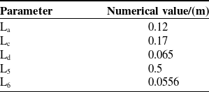


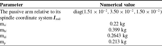


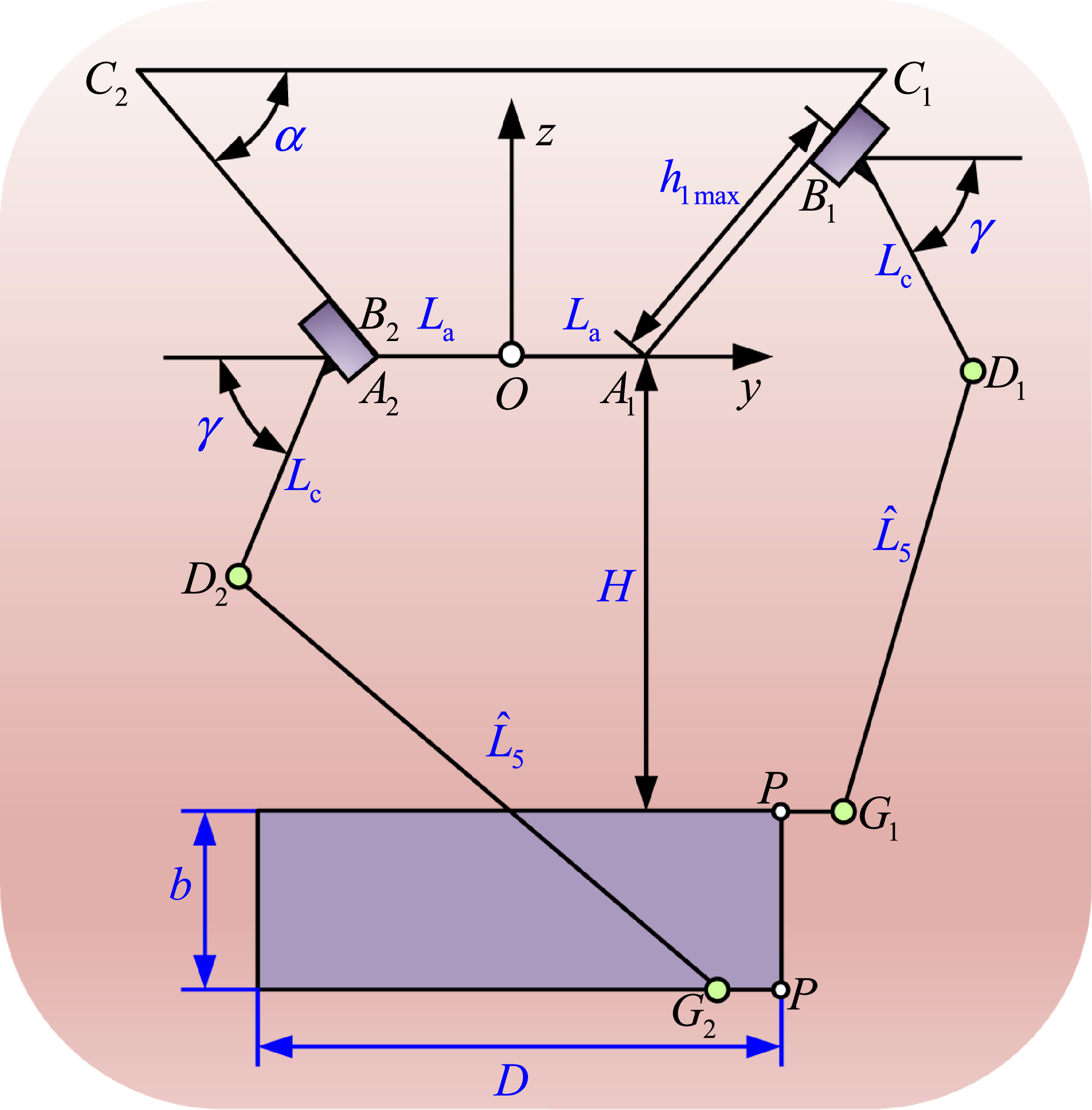

 α=π/4rad
 FaG,FvG,FgG
 La
 H
 L5=450mm
 L5=470mm
 L5=500mm

 L5=500mm
 FaG,FvG,FgG
 La
 H
 α=π/6
 α=5π/24
 α=π/4

 maxr∈Wt(σmax(J)),minr∈Wt(σmin(J))
 La
 H

 wGTFG,[Au],[Ad]
 hmax
 La
 H