





1. Introduction
1.1. Remote effect in dynamo action
In dynamo theory, the self-generation of a magnetic field from the motion of an electrically conducting fluid is generally thought to be localised in space, as suggested by the fast dynamo mechanism in which the stretching, twisting and folding of the magnetic field by the fluid motion, all occur at the same place (Vainshtein & Zel’dovich Reference Vainshtein and Zel’dovich1972; Childress & Gilbert Reference Childress and Gilbert1995). When the magnetic Reynolds number is high, the dynamo process then takes place within thin magnetic boundary layers, as is well documented for the Ponomarenko and Roberts dynamos (Soward Reference Soward1987; Gilbert Reference Gilbert1988; Ruzmaikin, Sokoloff & Shukurov Reference Ruzmaikin, Sokoloff and Shukurov1988; Gilbert Reference Gilbert2003; Tobias Reference Tobias2021). However, this aspect of spatial confinement is not mandatory, as is the case, for example, with the Herzenberg dynamo (Herzenberg Reference Herzenberg1958), which consists of two differential rotations (
 $\omega ^2$
dynamo) situated at a certain distance from one another. Another example is the mean-field dynamo (Steenbeck, Krause & Rädler Reference Steenbeck, Krause and Rädler1966; Krause & Rädler Reference Krause and Rädler1980), which is typically composed of two
 $\alpha$
effects (
 $\alpha ^2$
dynamo) or one
 $\alpha$
effect and one differential rotation (
 $\alpha \omega$
dynamo). Each mechanism considered alone (a simple differential rotation
 $\omega$
or an
 $\alpha$
effect) cannot produce the dynamo on its own, but the interplay of two of them,
 $\alpha ^2$
or
 $\alpha \omega$
, is sufficient to generate a magnetic field, even if they are distant from each other. If they do not operate in the same location, the transmission of electric currents from one place to another requires them to be electrically connected – generally considered to be part of the same electrically conducting medium. Such interplay of two distant mechanisms is also believed to be at work in the solar dynamo. The tachocline at the basis of the convection zone is the obvious site for differential rotation, while the
 $\alpha$
effect is considered to be located either near the surface or distributed throughout the convection zone (Weiss & Thompson Reference Weiss and Thompson2009; Jones, Thompson & Tobias Reference Jones, Thompson and Tobias2010). Of course, the greater the distance between the two locations, the less efficient the dynamo will be. To take a simple example, in the disc dynamo of Bullard (Reference Bullard1955), two mechanisms are also at work: the shear between the rotating rim of the disc and the wire, and the effect of the wound part of the wire (the loop) that is at some distance from the disc. The dynamo threshold expressed in terms of the angular velocity of the disc is
 $\varOmega =R/M$
, where
 $R$
and
 $M$
are respectively the electric resistance of the wire and the mutual inductance between the loop and the disc (Moffatt Reference Moffatt1978). If we denote the distance between the disc and the loop by
 $d$
, then
 $M$
decreases and
 $R$
increases linearly with
 $d$
, implying that the dynamo threshold increases as
 $d^2$
.
1.2. Anisotropic dynamo
After several decades during which the experimental implementation of the Bullard dynamo was considered impossible, mainly due to the high resistance of the electrical contact between the disc and the wire (Rädler & Rheinhardt Reference Rädler and Rheinhardt2002), a decisive breakthrough was achieved by Priede & Avalos-Zúñiga (Reference Priede and Avalos-Zúñiga2013), who, instead of a single wire, proposed using a spiral-segmented disc and an electrical contact extending around the entire circumference of the disc. In their theroretical model, the spiral-segmented disc is replaced by a material exhibiting anisotropic electrical conductivity. As Cowling’s anti-dynamo theorem (Cowling Reference Cowling1934) no longer applies, it can then be assumed that the magnetic mode is axisymmetric – a common assumption in subsequent models of anisotropic dynamos (Alboussière et al. Reference Alboussière, Drif and Plunian2020; Plunian & Alboussière Reference Plunian and Alboussière2020). The concept of the anisotropic dynamo has been independently confirmed by two experimental demonstrations based on different geometries (Alboussière et al. Reference Alboussière, Plunian and Moulin2022; Avalos-Zúñiga & Priede Reference Avalos-Zúñiga and Priede2023).
In the anisotropic dynamo, two distinct mechanisms are at work; one being the deflection of electric currents by the presence of a material having an anisotropic electrical conductivity – we speak of an anisotropic material; the other being, in its simplest form, shear. Once again, simple shearing cannot generate a magnetic field; it is the combination of shear with the anisotropic material that creates the dynamo effect. We note that an anisotropy of magnetic permeability also works (Plunian & Alboussière Reference Plunian and Alboussière2021), implying a deflection of the magnetic field instead. Furthermore, there is a necessary condition between the direction of anisotropy and that of shear, just as in Bullard’s disc dynamo, the direction of rotation of the disc, and that of the wire winding. In other words, for a given anisotropy, there is only one direction of shear for which the dynamo works.
In the Fury dynamo experiment (Alboussière et al. Reference Alboussière, Plunian and Moulin2022), a rotor rotates inside a stator, both of which are cylindrical in shape and made of the same anisotropic material. Although a layer of an electrically conducting fluid is sandwiched between the rotor and the stator to ensure good electric contact, it is so thin (1 % of the rotor radius) that it can be disregarded when calculating the dynamo threshold. The angular velocity profile thus corresponds to a Heaviside step function. A smooth profile also works and has been studied in the context of fast dynamo action (Plunian & Alboussière Reference Plunian and Alboussière2022) and spiral galaxies (Gomez, Plunian & Alboussière Reference Gomez, Plunian and Alboussière2025). As part of the preparation for another dynamo experiment, the effect of the fluid layer thickness was also investigated (Plunian, Gomez & Alboussière Reference Plunian, Gomez and Alboussière2025). Within a fluid, because the electrical conductivity is isotropic, the electric currents are not deflected, and therefore, do not contribute directly to the dynamo mechanism. The dynamo threshold thus inevitably increases with the fluid thickness, but still works even in the limit of infinite thickness (Plunian & Alboussière Reference Plunian and Alboussière2023).
In these studies, the shear was always taken in contact with the anisotropic material, even in the cases involving a fluid. This raises the question of whether the dynamo would work if, instead, the shear occurred within the fluid, and therefore, at some distance from the anisotropic material. In this case, the electric currents would be deflected only at a certain distance from the shear, making the dynamo more difficult to achieve. This is, however, of fundamental importance, as shear does not necessarily occur at the walls of a fluid.
1.3. Outline
We examine three configurations based on the number of solid components: one rotor (case A), one stator (case B), and one rotor and one stator (case C), all made from the same anisotropic material. Space is therefore divided into three domains in cases A and B, and four domains in case C, as shown in figure 1. The increase of the number of domains increases the number of boundary conditions (§ 3), which leads to a system of eight (respectively twelve) equations to be solved in cases A and B (respectively C), as derived in § 4. An explicit expression for the dynamo threshold is obtained in each of these three cases (§ 5), and a number of checks can be carried out, on the basis of previous studies or by comparing case C with case A or B, as outlined in § 6. Finally, in § 7 we investigate how the dynamo threshold varies with the distance between the shear and the anisotropic material for three applications chosen for their relevance to past or future experiments. We also estimate the degree of anisotropy that would be necessary to produce a dynamo effect from simple shear within the Earth’s liquid outer core iron, if the inner core were made of anisotropic solid iron.
A non-zero angular velocity
 $\varOmega$
is represented by a vertical elevation. The fluid layer is represented in grey and divided into two parts: one is rotating, the other is at rest. The anisotropic material is represented with logarithmic spirals, the rotor in case A (a), the stator in case B (b), both rotor and stator in case C (c). (a) Case A: the fluid inner part (
 $R \lt r \lt R+e$
) rotates at the same angular velocity as the rotor (
 $r\lt R$
). The fluid outer part (
 $r \gt R+e$
) is at rest. Shear occurs at radius
 $r=R+e$
. (b) Case B: the fluid (
 $r\lt R+e$
) is surrounded by a stator (
 $r \gt R+e$
) at rest. The fluid inner part (
 $r\lt R$
) rotates, while the fluid outer part (
 $R\lt r \lt R+e$
) is at rest. Shear occurs at radius
 $r=R$
. (c) Case C: the fluid layer is sandwiched between a rotor (
 $r\lt R$
) and a stator (
 $r \gt R+e$
). The fluid inner part (
 $R\lt r\lt R+e_1$
) rotates at the same angular velocity as the rotor. The fluid outer part (
 $R+e_1\lt r\lt R+e$
) is at rest as the stator. Shear occurs at radius
 $r=R+e_1$
. The logarithmic spirals in the rotor (cases A and C) and the stator (cases B and C) correspond to the direction of the electric current (respectively magnetic field) for
 $\sigma ^{\perp }\gg \sigma ^{\parallel }$
(respectively
 $\mu ^{\perp }\gg \mu ^{\parallel }$
), which are perpendicular to
 $\boldsymbol{{q}}$
.

Figure 1. Long description
Panel A: A diagram showing a fluid layer divided into an inner rotating part and an outer part at rest. The inner part rotates with the same angular velocity as the rotor. Shear occurs at radius R. The anisotropic material is represented by logarithmic spirals indicating the direction of electric current. Panel B: A diagram showing a fluid layer surrounded by a stator at rest. The inner part of the fluid rotates, while the outer part is at rest. Shear occurs at radius R. The anisotropic material is represented by logarithmic spirals indicating the direction of the magnetic field. Panel C: A diagram showing a fluid layer sandwiched between a rotor and a stator. The inner part of the fluid rotates with the same angular velocity as the rotor, while the outer part is at rest as the stator. Shear occurs at radius R. The logarithmic spirals in the rotor and stator correspond to the direction of the electric current and magnetic field, respectively.
2. General formulation
2.1. Shear
To solve the problem analytically, the shear within the fluid layer will be treated in its simplest form, namely a Heaviside step function, with one part being at rest and the other one having a non-zero angular velocity (figure 1). To implement the remote effect of electrical conductivity (or magnetic permeability) anisotropy, we consider one rotor (case A), one stator (case B), or both one rotor and one stator (case C), located at a certain distance
 $e$
(case A and B), or
 $e_1$
and
 $e-e_1$
(case C), from the shear (figure 1).
In cases A and B, space is therefore divided into three cylindrical regions:
 $r \lt R$
,
 $R\lt r \lt R+e$
and
 $r \gt R+e$
, where
 $r$
is the radial coordinate, as illustrated in figures 1(a) and 1(b). Only one part, the rotor in case A and the stator in case B, is made of an anisotropic material. In case A the fluid inner part (
 $R \lt r \lt R+e$
) rotates at the same angular velocity
 $\varOmega$
as the rotor, while the fluid outer part (
 $r \gt R+e$
) is at rest. In case B the fluid outer part (
 $R \lt r \lt R+e$
) is at rest as the stator, while the inner part (
 $r\lt R$
) rotates at angular velocity
 $\varOmega$
. Therefore, in both cases, the shear occurs in the fluid layer at a distance
 $e$
from the anisotropic medium, namely at (a)
 $r=R+e$
or (b)
 $r=R$
.
In case C, space is divided into four cylindrical regions:
 $r \lt R, R\lt r \lt R+e_1$
,
 $R+e_1\lt r \lt R+e$
and
 $r \gt R+e$
, the fluid layer corresponding to the two intermediate parts
 $R\lt r \lt R+e_1$
and
 $R+e_1\lt r \lt R+e$
, as illustrated in figure 1(c). Both the rotor (
 $r \lt R$
) and the stator (
 $r \gt R+e$
) are made of the same anisotropic material. The inner part of the fluid layer (
 $R\lt r\lt R+e_1$
) rotates at the same angular velocity as the rotor, while the outer part (
 $R+e_1\lt r\lt R+e$
) is at rest as the stator. The shear then occurs at a distance
 $e_1$
from the rotor and
 $e-e_1$
from the stator, namely at
 $r=R+e_1$
.
In cases A and B, setting
 $e=0$
corresponds to a shear at the interface
 $r=R$
, between the fluid layer and the anisotropic material, which has already been studied in Plunian & Alboussière (Reference Plunian and Alboussière2023). In case C, setting
 $e_1=0$
, or
 $e-e_1=0$
, corresponds to the two cases studied in Plunian et al. (Reference Plunian, Gomez and Alboussière2025), with a shear at the interface between the fluid layer and either the rotor at
 $r=R$
or the stator at
 $r=R+e_1$
. In cases A and B, for
 $e\gg 1$
, the shear is pushed to an infinitely large distance from the anisotropic material, which makes the dynamo effect impossible. We therefore expect that an increase in
 $e$
will lead to an increase in the dynamo threshold. In case C, similarly, we expect an increase of the dynamo threshold for
 $e\gg e_1\gg 1$
. For the applications discussed in § 7,
 $e$
will be of the same order of magnitude as the rotor radius
 $e=O(R)$
.
The velocity field is given by
 $\boldsymbol{{U}}=r\tilde {\varOmega } \boldsymbol{{e}}_{\theta }$
, with
 \begin{eqnarray} \tilde {\varOmega }^{({\rm A})}= \left \{ \begin{split} &\varOmega & \\ &\varOmega \\ &0 & \end{split}\!\!,\;\;\; \right . \tilde {\varOmega }^{({\rm B})}= \left \{ \begin{split} &\varOmega & \\ &0 & \\ &0 & \end{split}\!\!\!\!,\;\;\; \right . \text{for} \left \{\begin{split} &0\lt r\lt R \\ &R\lt r\lt R+e\\ &r\gt R+e \end{split}\,, \right . \end{eqnarray}
 \begin{eqnarray} \tilde {\varOmega }^{({\rm C})}= \left \{ \begin{split} &\varOmega \\ &\varOmega \\ &0 \\ &0 \end{split}\,,\;\;\; \right . \text{for} \left \{\begin{split} &0\lt r\lt R \\ &R\lt r\lt R+e_1\\ &R+e_1\lt r\lt R+e\\ &r\gt R+e \end{split}\;\;\;, \right . \end{eqnarray}
where
 $(\boldsymbol{{e}}_r,\boldsymbol{{e}}_{\theta },\boldsymbol{{e}}_z)$
and
 $(r, \theta , z)$
are unit basis vectors and coordinates in cylindrical geometry, and where the superscripts
 $({\rm A}), ({\rm B})$
and
 $({\rm C})$
correspond to the three cases introduced above and depicted in figure 1.
2.2. Anisotropy
In each domain, we define two electrical conductivities and two magnetic permeabilities,
 $\sigma ^{\parallel }$
and
 $\mu ^{\parallel }$
in a given direction
 $\boldsymbol{{q}}$
,
 $\sigma ^{\perp }$
and
 $\mu ^{\perp }$
in the directions perpendicular to
 $\boldsymbol{{q}}$
, where
 $\boldsymbol{{q}}$
is a unit vector. In the direction parallel to
 $\boldsymbol{{q}}$
, Ohm’s law and the relation between
 $\boldsymbol{{H}}$
and
 $\boldsymbol{{B}}$
are written in the formFootnote
1
 $\boldsymbol{{J}}\boldsymbol{\cdot }\boldsymbol{{q}}=\sigma ^{\parallel } (\boldsymbol{{E}}\boldsymbol{\cdot }\boldsymbol{{q}})$
and
 $\boldsymbol{{B}}\boldsymbol{\cdot }\boldsymbol{{q}}=$
 $\mu ^{\parallel }(\boldsymbol{{H}}\boldsymbol{\cdot }\boldsymbol{{q}})$
, while in the directions perpendicular to
 $\boldsymbol{{q}}$
they are written as
 $\boldsymbol{{J}}-(\boldsymbol{{J}}\boldsymbol{\cdot }\boldsymbol{{q}})$
 $\boldsymbol{{q}}=\sigma ^{\perp } (\boldsymbol{{E}}-(\boldsymbol{{E}}\boldsymbol{\cdot }\boldsymbol{{q}})\boldsymbol{{q}})$
and
 $\boldsymbol{{B}}-(\boldsymbol{{B}}\boldsymbol{\cdot }\boldsymbol{{q}})\boldsymbol{{q}}=\mu ^{\perp }(\boldsymbol{{H}}-(\boldsymbol{{H}}\boldsymbol{\cdot }\boldsymbol{{q}})\boldsymbol{{q}})$
. This leads to two symmetric tensors,
 $\lbrack \sigma _{ij}\rbrack$
for the electrical conductivity and
 $\lbrack \mu _{ij}\rbrack$
for the magnetic permeability, defined by
 \begin{align} \lbrack \sigma _{ij}\rbrack =\sigma ^{\perp } \delta _{ij} + (\sigma ^{\parallel }-\sigma ^{\perp })q_i q_j, \;\;\;\;\;\;\;\;\; \lbrack \mu _{ij}\rbrack =\mu ^{\perp } \delta _{ij} + (\mu ^{\parallel }-\mu ^{\perp })q_i q_j. \end{align}
For a fluid, with isotropic electrical conductivity
 $\sigma _F$
and magnetic permeability
 $\mu _F$
, the expressions (2.2a
,
b
) remain valid, with
 $\sigma ^{\perp }=\sigma ^{\parallel }=\sigma _F$
and
 $\mu ^{\perp }=\mu ^{\parallel }=\mu _F$
. Anticipating a renormalisation of the electrical conductivity and magnetic permeability by
 $\sigma ^{\perp }_{\rm }$
and
 $\mu ^{\perp }_{\rm }$
, it is then useful to rewrite (2.2a
,
b
) as
 \begin{align} \lbrack \sigma _{ij}\rbrack =\sigma ^{\perp }_{\rm }\; \tilde {\varphi }_{\sigma } \left (\delta _{ij} -\frac {\tilde {\sigma }}{1+\tilde {\sigma }}q_i q_j\right ), \;\;\;\;\;\;\;\;\; \lbrack \mu _{ij}\rbrack =\mu ^{\perp }_{\rm }\; \tilde {\varphi }_{\mu } \left (\delta _{ij} -\frac {\tilde {\mu }}{1+\tilde {\mu }}q_i q_j\right ), \end{align}
with, in case A,
 \begin{align} \tilde {\varphi }_{\sigma }^{({\rm A})}= \left \{ {\begin{matrix} &1 \\ &\varphi _{\sigma } \\ &\varphi _{\sigma } \end{matrix}} \right . , \quad \tilde {\sigma }^{({\rm A})}= \left \{ {\begin{matrix} &\sigma \\ &0\\ &0 \end{matrix}} \right . , \quad \tilde {\varphi }_{\mu }^{({\rm A})}= \left \{ {\begin{matrix} &1 \\ &\varphi _{\mu }\\ &\varphi _{\mu } \end{matrix}} \right . , \quad \tilde {\mu }^{({\rm A})}= \left \{ {\begin{matrix} &\mu \\ &0\\ &0 \end{matrix}} \right . , \quad \text{for} \left \{ {\begin{array}{l} r\lt R \\ R\lt r\lt R+e\\ r\gt R+e \end{array}}\right. ,\end{align}
in case B,
 \begin{align} \tilde {\varphi }_{\sigma }^{({\rm B})}= \left \{ \begin{matrix} &\varphi _{\sigma } \\ &\varphi _{\sigma } \\ &1 \end{matrix} \right . ,\quad \tilde {\sigma }^{({\rm B})}= \left \{ \begin{matrix} &0 \\ &0\\ &\sigma \end{matrix} \right . , \quad \tilde {\varphi }_{\mu }^{({\rm B})}= \left \{ \begin{matrix} &\varphi _{\mu } \\ &\varphi _{\mu }\\ &1 \end{matrix} \right . , \quad \tilde {\mu }^{({\rm B})}= \left \{ \begin{matrix} &0 \\ &0\\ &\mu \end{matrix} \right . , \quad \text{for} \left \{ {\begin{array}{l} r\lt R \\ R\lt r\lt R+e\\ r\gt R+e \end{array}}\right. , \end{align}
in case C,
 \begin{align} \tilde {\varphi }_{\sigma }^{({\rm C})}= \left \{ \begin{matrix} &1\\ &\varphi _{\sigma } \\ &\varphi _{\sigma } \\ &1 \end{matrix} \right . , \quad\! \tilde {\sigma }^{({\rm C})}= \left \{ \begin{matrix} &\sigma \\ &0 \\ &0\\ &\sigma \end{matrix} \right . , \quad\! \tilde {\varphi }_{\mu }^{({\rm C})}= \left \{ \begin{matrix} &1\\ &\varphi _{\mu } \\ &\varphi _{\mu }\\ &1 \end{matrix} \right . , \quad\!\! \tilde {\mu }^{({\rm C})}= \left \{ \begin{matrix} &\mu \\ &0 \\ &0\\ &\mu \end{matrix} \right . , \quad\!\! \text{for} \; \left \{ {\begin{array}{l} r\lt R \\ R\lt r\lt R+e_1\\ R+e_1\lt r\lt R+e\\ r\gt R+e \end{array}}\right. , \end{align}
and
 \begin{align} \varphi _{\sigma }=\frac {\sigma _F}{\sigma ^{\perp }}, \;\;\;\; \sigma =\frac {\sigma ^{\perp }}{\sigma ^{\parallel }}-1, \;\;\;\; \varphi _{\mu }=\frac {\mu _F}{\mu ^{\perp }}, \;\;\;\; \mu =\frac {\mu ^{\perp }}{\mu ^{\parallel }}-1.\end{align}
As in previous studies on the anisotropic dynamo (Plunian & Alboussière Reference Plunian and Alboussière2020, Reference Plunian and Alboussière2021, Reference Plunian and Alboussière2022, Reference Plunian and Alboussière2023; Gomez et al. Reference Gomez, Plunian and Alboussière2025; Plunian et al. Reference Plunian, Gomez and Alboussière2025), we choose
 $\boldsymbol{{q}}$
as a unit vector in the horizontal plane defined by
 \begin{equation} \boldsymbol{{q}}=c \; \boldsymbol{{e}}_r+s \; \boldsymbol{{e}}_{\theta }, \end{equation}
where
 $c=\cos \alpha _q$
,
 $s=\sin \alpha _q$
, with
 $\alpha _q$
a prescribed pitch angle. The vector
 $\boldsymbol{{q}}$
follows the direction of logarithmic spirals that are perpendicular to those depicted in figure 1 (see Ruderman & Ruzmaikin Reference Ruderman and Ruzmaikin1984; Alboussière et al. Reference Alboussière, Drif and Plunian2020 for an alternative expression in Cartesian geometry).
2.3. Induction equation
In the magnetohydrodynamic approximation, Maxwell’s equations and Ohm’s law take the forms
 \begin{align} \boldsymbol{{H}}&=\lbrack \mu _{ij}\rbrack ^{-1}\boldsymbol{{B}},\\[-10pt]\nonumber \end{align}
 \begin{align} \boldsymbol{\nabla }\boldsymbol{\cdot }\boldsymbol{{B}} &= 0,\\[-10pt]\nonumber \end{align}
 \begin{align} \boldsymbol{{J}}&=\boldsymbol{\nabla }\times \boldsymbol{{H}},\\[-10pt]\nonumber \end{align}
 \begin{align} \partial _t \boldsymbol{{B}} &= - \boldsymbol{\nabla }\times \boldsymbol{{E}}\\[-10pt]\nonumber \end{align}
 \begin{align} \boldsymbol{{J}}&=\lbrack \sigma _{ij}\rbrack (\boldsymbol{{E}} + \boldsymbol{{U}} \times \boldsymbol{{B}}), \end{align}
leading to the induction equation,
 \begin{equation} \partial _t \boldsymbol{{B}} = \boldsymbol{\nabla }\times (\boldsymbol{{U}} \times \boldsymbol{{B}}) - \boldsymbol{\nabla }\times \left ( \lbrack \sigma _{ij}\rbrack ^{-1} \boldsymbol{\nabla }\times \left ( \lbrack \mu _{ij}\rbrack ^{-1}\boldsymbol{{B}} \right ) \right ), \end{equation}
where
 \begin{align} \lbrack \sigma _{ij}\rbrack ^{-1}=\left (\tilde {\varphi }_{\sigma }\sigma ^{\perp }\right )^{-1} \left (\delta _{ij} + \tilde {\sigma } q_i q_j \right ), \;\;\;\;\;\;\;\;\; \lbrack \mu _{ij}\rbrack ^{-1}= \left (\tilde {\varphi }_{\mu }\mu ^{\perp }\right )^{-1} \left (\delta _{ij} + \tilde {\mu } q_i q_j \right ).\end{align}
Equations (2.11a,b
) have been derived from (2.3a,b
) knowing that, for any unit vector
 $\boldsymbol{{q}}$
and any scalar quantity
 $X \neq -1$
, we have
 \begin{equation} \left [\delta _{ij} -\frac {X}{1+X}q_i q_j\right ]^{-1} = \delta _{ij} + X q_i q_j. \end{equation}
With regard to the induction equation (2.10), and for an isotropic material such that
 $\lbrack \sigma _{ij}\rbrack$
and
 $\lbrack \mu _{ij}\rbrack$
are reduced to scalar quantities, it has been shown, using duality arguments, that swapping the electrical conductivity and magnetic permeability leads to the same dynamo threshold, provided that there is a change of sign in the velocity field and that the boundary conditions of the conducting domain can also be swapped (infinitely conducting with ferromagnetic) (Favier & Proctor Reference Favier and Proctor2013; Marcotte et al. Reference Marcotte, Gallet, Pétrélis and Gissinger2021). This demonstration can easily be generalised to the current case of an anisotropic material, and for the boundary conditions (3.1c–d
) given in § 3.1. Consequently, we expect to have the same dynamo threshold by swapping
 $\sigma$
and
 $\mu$
,
 $\varphi _{\sigma }$
and
 $\varphi _{\mu }$
,
 $\varOmega$
and
 $-\varOmega$
.
Since the velocity is stationary and independent of
 $z$
and
 $\theta$
, we look for a magnetic induction in the form
 \begin{equation} \boldsymbol{{B}}(r)\exp (\gamma t + \mathrm{i} kz+im\theta ), \end{equation}
where
 $\boldsymbol{{B}}(r)$
is the magnetic mode at vertical wavenumber
 $k$
and azimuthal wavenumber
 $m$
. In (2.13) a positive value of the real part of the magnetic growth rate
 $\gamma$
is the signature of dynamo action, the dynamo threshold corresponding to
 $\Re \{\gamma \}=0$
. The present work is restricted to the axisymmetric mode
 $m=0$
, motivated by the fact that it does not involve azimuthal gradients and is therefore the least dissipative candidate. This is also consistent with previous experimental studies of anisotropic dynamo (Alboussière et al. Reference Alboussière, Plunian and Moulin2022; Avalos-Zúñiga & Priede Reference Avalos-Zúñiga and Priede2023) in which the magnetic field is indeed axisymmetric. As mentioned in § 1.2, the generation of an axisymmetric mode
 $m=0$
is possible because in the anisotropic material the electric currents are deflected, implying that Cowling’s antidynamo theorem (Cowling Reference Cowling1934) does not hold (Plunian & Alboussière Reference Plunian and Alboussière2020).
Replacing (2.1a
), (2.1b
) and (2.13) in (2.10), and after some algebra (see, e.g. Plunian & Alboussière Reference Plunian and Alboussière2023), we obtain the following equations for
 $B_r(r)$
and
 $B_{\theta }(r)$
:
 \begin{align} \tilde {\gamma } B_r &= -(\sigma ^{\perp }\mu ^{\perp })^{-1} \big[ \tilde {\mu } c^2 k^2 B_r + (1+\tilde {\sigma } s^2) D_k(B_r) - cs(\tilde {\sigma } -\tilde {\mu }) k^2 B_{\theta } \big],\\[-7pt]\nonumber \end{align}
 \begin{align} \tilde {\gamma } B_{\theta } &= -(\sigma ^{\perp }\mu ^{\perp })^{-1} \left [ \tilde {\sigma } c^2 k^2 B_{\theta } + (1+\tilde {\mu } s^2)D_k (B_{\theta }) - cs(\tilde {\sigma } -\tilde {\mu }) D_k(B_r) \right ] . \end{align}
Here
 $\tilde {\gamma }=\tilde {\varphi }_{\sigma }\tilde {\varphi }_{\mu }\gamma$
is given by
 \begin{eqnarray} \tilde {\gamma }^{({\rm A})}=\gamma \left \{ \begin{split} &1& \\ &\varphi _{\sigma }\varphi _{\mu } \\ &\varphi _{\sigma }\varphi _{\mu }& \end{split}\!\!\!, \right . \;\;\; \tilde {\gamma }^{({\rm B})}=\gamma \left \{ \begin{split} &\varphi _{\sigma }\varphi _{\mu } \\ &\varphi _{\sigma }\varphi _{\mu } \\ &1 \end{split} \right . , \;\;\;\text{for} \left \{ \begin{split} & r\lt R \\ & R\lt r\lt R+e \\ & r\gt R+e \end{split} \right .\! , \end{eqnarray}
 \begin{eqnarray} \tilde {\gamma }^{({\rm C})}=\gamma \left \{ \begin{split} &1\\ &\varphi _{\sigma }\varphi _{\mu } \\ &\varphi _{\sigma }\varphi _{\mu } \\ &1 \end{split} \right . ,\;\;\; \text{for} \;\;\; \left \{ \begin{split} &r\lt R\\ &R\lt r\lt R+e_1 \\ &R+e_1\lt r\lt R+e \\ &r\gt R+e \end{split} \right . , \end{eqnarray}
and
 \begin{equation} D_{k}(X)=k^2X-\frac {\partial }{\partial r}\left (\frac {1}{r}\frac {\partial }{\partial r}(rX)\right ). \end{equation}
3. Boundary conditions and renormalisation
3.1. Boundary conditions
The system of equations (2.14a,b
) is completed by the appropriate boundary conditions for
 $r=0$
and
 $r\rightarrow \infty$
,
 \begin{align} B_r(r=0)= B_{\theta }(r=0)= \lim _{r\rightarrow \infty }B_r=\lim _{r\rightarrow \infty }B_{\theta } = 0,\end{align}
and by the continuity across
 $r=R$
and
 $r=R+e$
of the normal component of
 $\boldsymbol{{B}}$
and of the tangential components of
 $\boldsymbol{{H}}$
and
 $\boldsymbol{{E}}$
,
 \begin{align} \left [B_r\right ]^{R^+}_{R^-} = \left [H_{\theta }\right ]^{R^+}_{R^-} =\left [H_z\right ]^{R^+}_{R^-} =\left [E_{\theta }\right ]^{R^+}_{R^-} =\left [E_z\right ]^{R^+}_{R^-} =0,\\[-10pt]\nonumber \end{align}
 \begin{align} \left [B_r\right ]^{(R+e)^+}_{(R+e)^-} = \left [H_{\theta }\right ]^{(R+e)^+}_{(R+e)^-} =\left [H_z\right ]^{(R+e)^+}_{(R+e)^-} =\left [E_{\theta }\right ]^{(R+e)^+}_{(R+e)^-} =\left [E_z\right ]^{(R+e)^+}_{(R+e)^-} =0,\end{align}
and for case C, by the continuity across
 $r=R+e_1$
of the same quantities,
 \begin{align} \left [B_r\right ]^{(R+e_1)^+}_{(R+e_1)^-} = \left [H_{\theta }\right ]^{(R+e_1)^+}_{(R+e_1)^-} =\left [H_z\right ]^{(R+e_1)^+}_{(R+e_1)^-} =\left [E_{\theta }\right ]^{(R+e_1)^+}_{(R+e_1)^-} =\left [E_z\right ]^{(R+e_1)^+}_{(R+e_1)^-} =0,\end{align}
where
 $[X]^{r_2}_{r_1} =X(r=r_2)-X(r=r_1)$
.
From (2.9a
) and (2.11b
), the magnetic field
 $\boldsymbol{{H}}$
takes the form
 \begin{equation} \boldsymbol{{H}}=\left (\tilde {\varphi }_{\mu }\mu ^{\perp }\right )^{-1}\begin{pmatrix} (1+\tilde {\mu } c^2)B_r+ \tilde {\mu } cs B_{\theta }\\[3pt] \tilde {\mu } cs B_r + (1+\tilde {\mu } s^2)B_{\theta }\\[3pt] B_z \end{pmatrix}, \end{equation}
with, from (2.9b ),
 \begin{equation} B_z = \mathrm{i} k^{-1} \left(\frac {B_r}{r}+\frac {\partial B_r}{\partial r}\right). \end{equation}
Then (3.2a – c ) and (3.3a – c ) can be rewritten, in case A, as
 \begin{eqnarray} &B_r^{({\rm A})}(R^+)=B_r^{({\rm A})}(R^-),\end{eqnarray}
 \begin{eqnarray} &\varphi _{\mu }^{-1}B_{\theta }^{({\rm A})}(R^+) =\mu cs B_r^{({\rm A})}(R^-)+(1+\mu s^2)B_{\theta }^{({\rm A})}(R^-), \end{eqnarray}
 \begin{eqnarray} &\varphi _{\mu }^{-1}\left (\frac {B_r^{({\rm A})}(R^+)}{R} + \frac {\partial B_r^{({\rm A})}}{\partial r}(R^+)\right )=\frac {B_r^{({\rm A})}(R^-)}{R} + \frac {\partial B_r^{({\rm A})}}{\partial r}(R^-), \end{eqnarray}
 \begin{eqnarray} &B_r^{({\rm A})}((R+e)^-)=B_r^{({\rm A})}((R+e)^+), \end{eqnarray}
 \begin{eqnarray} &B_{\theta }^{({\rm A})}((R+e)^-) =B_{\theta }^{({\rm A})}((R+e)^+),\end{eqnarray}
 \begin{align} \frac {B_r^{({\rm A})}((R+e)^-)}{(R+e)} + \frac {\partial B_r^{({\rm A})}}{\partial r}((R+e)^-)=\frac {B_r^{({\rm A})}((R+e)^+)}{(R+e)} + \frac {\partial B_r^{({\rm A})}}{\partial r}((R+e)^+), \end{align}
in case B, as
 \begin{eqnarray} &B_r^{({\rm B})}(R^+)=B_r^{({\rm B})}(R^-), \end{eqnarray}
 \begin{eqnarray} &B_{\theta }^{({\rm B})}(R^+) =B_{\theta }^{({\rm B})}(R^-), \end{eqnarray}
 \begin{eqnarray} &\frac {B_r^{({\rm B})}(R^+)}{R} + \frac {\partial B_r^{({\rm B})}}{\partial r}(R^+)=\frac {B_r^{({\rm B})}(R^-)}{R} + \frac {\partial B_r^{({\rm B})}}{\partial r}(R^-) ,\end{eqnarray}
 \begin{eqnarray} &B_r^{({\rm B})}((R+e)^-)=B_r^{({\rm B})}((R+e)^+) ,\end{eqnarray}
 \begin{eqnarray} &\varphi _{\mu }^{-1}B_{\theta }^{({\rm B})}((R+e)^-) =\mu cs B_r^{({\rm B})}((R+e)^+) +(1+\mu s^2) B_{\theta }^{({\rm B})}((R+e)^+), \end{eqnarray}
 \begin{align} \varphi _{\mu }^{-1}\left (\frac {B_r^{({\rm B})}((R+e)^-)}{(R+e)} + \frac {\partial B_r^{({\rm B})}}{\partial r}((R+e)^-)\right )=\frac {B_r^{({\rm B})}((R+e)^+)}{(R+e)} + \frac {\partial B_r^{({\rm B})}}{\partial r}((R+e)^+). \end{align}
In case C, (3.2a – c ), (3.3a – c ) and (3.4a – c ) can be rewritten as
 \begin{eqnarray} &B_r^{({\rm C})}(R^+)=B_r^{({\rm C})}(R^-), \end{eqnarray}
 \begin{eqnarray} &\varphi _{\mu }^{-1}B_{\theta }^{({\rm C})}(R^+) =\mu cs B_r^{({\rm C})}(R^-)+(1+\mu s^2)B_{\theta }^{({\rm C})}(R^-), \end{eqnarray}
 \begin{eqnarray} &\varphi _{\mu }^{-1}\left (\frac {B_r^{({\rm C})}(R^+)}{R} + \frac {\partial B_r^{({\rm C})}}{\partial r}(R^+)\right )=\frac {B_r^{({\rm C})}(R^-)}{R} + \frac {\partial B_r^{({\rm C})}}{\partial r}(R^-) ,\end{eqnarray}
 \begin{eqnarray} &B_r^{({\rm C})}((R+e_1)^+)=B_r^{({\rm C})}((R+e_1)^-) ,\end{eqnarray}
 \begin{eqnarray} &B_{\theta }^{({\rm C})}((R+e_1)^+) =B_{\theta }^{({\rm C})}((R+e_1)^-) ,\end{eqnarray}
 \begin{align} \frac {B_r^{({\rm C})}((R+e_1)^+)}{R+e_1} + \frac {\partial B_r^{({\rm C})}}{\partial r}((R+e_1)^+)=\frac {B_r^{({\rm C})}((R+e_1)^-)}{R+e_1} + \frac {\partial B_r^{({\rm C})}}{\partial r}((R+e_1)^-) ,\end{align}
 \begin{eqnarray} &B_r^{({\rm C})}((R+e)^-)=B_r^{({\rm C})}((R+e)^+) ,\end{eqnarray}
 \begin{eqnarray} &\varphi _{\mu }^{-1}B_{\theta }^{({\rm C})}((R+e)^-) =\mu cs B_r^{({\rm C})}((R+e)^+) +(1+\mu s^2)B_{\theta }^{({\rm C})}((R+e)^+), \end{eqnarray}
 \begin{align} \varphi _{\mu }^{-1}\left (\frac {B_r^{({\rm C})}((R+e)^-)}{(R+e)} + \frac {\partial B_r^{({\rm C})}}{\partial r}((R+e)^-)\right )=\frac {B_r^{({\rm C})}((R+e)^+)}{(R+e)} + \frac {\partial B_r^{({\rm C})}}{\partial r}((R+e)^+). \end{align}
From (2.9d
) we have
 $E_{\theta }=-\mathrm{i} k^{-1}\gamma B_r$
, implying that the two conditions (3.2a
) and (3.2d
) are redundant, as are (3.3a
) and (3.3d
), and (3.4a
) and (3.4d
). As for the last boundary conditions (3.2e
), (3.3e
) and (3.4e
), using (2.9e
) we have
 \begin{equation} \tilde {\varphi }_{\sigma }^{-1}J_z + \sigma ^{\perp } r \tilde {\varOmega } B_r=\sigma ^{\perp }E_z \end{equation}
with
 $\tilde {\varOmega }$
defined in (2.1a
) and (2.1b
), leading to in case A,
 \begin{align} \varphi _{\sigma }^{-1}J_z^{({\rm A})}(R^+) + \sigma ^{\perp }\varOmega R B_r^{({\rm A})}(R^{+})= J_z^{({\rm A})}(R^-)+ \sigma ^{\perp } \varOmega R B_r^{({\rm A})}(R^{-}), \end{align}
 \begin{align} \varphi _{\sigma }^{-1}J_z^{({\rm A})}((R+e)^+)= \varphi _{\sigma }^{-1} J_z^{({\rm A})}((R+e)^-)+\sigma ^{\perp } \varOmega (R+e) B_r^{({\rm A})}((R+e)^{-}), \end{align}
in case B,
 \begin{align} \varphi _{\sigma }^{-1}J_z^{({\rm B})}(R^+) = \varphi _{\sigma }^{-1} J_z^{({\rm B})}(R^-)+ \sigma ^{\perp } \varOmega R B_r^{({\rm B})}(R^{-}), \end{align}
 \begin{align} J_z^{({\rm B})}((R+e)^+)= \varphi _{\sigma }^{-1} J_z^{({\rm B})}((R+e)^-), \end{align}
and in case C,
 \begin{align} \varphi _{\sigma }^{-1}J_z^{({\rm C})}(R^+) + \sigma ^{\perp }\varOmega R B_r^{({\rm C})}(R^{+})= J_z^{({\rm C})}(R^-)+ \sigma ^{\perp } \varOmega R B_r^{({\rm C})}(R^{-}), \end{align}
 \begin{align} \varphi _{\sigma }^{-1}J_z^{({\rm C})}((R+e_1)^+)= \varphi _{\sigma }^{-1} J_z^{({\rm C})}((R+e_1)^-)+\sigma ^{\perp } \varOmega (R+e_1) B_r^{({\rm C})}((R+e_1)^{-}), \end{align}
 \begin{align} J_z^{({\rm C})}((R+e)^+)= \varphi _{\sigma }^{-1} J_z^{({\rm C})}((R+e)^-). \end{align}
3.2. Magnetic Reynolds number and renormalisation
By defining the magnetic Reynolds number in terms of the radius
 $R$
, the angular velocity
 $\varOmega$
, the electrical conductivity and magnetic permeability,
 $\sigma ^{\perp }$
and
 $\mu ^{\perp }$
in cases A and C, and
 $\sigma ^{F}$
and
 $\mu ^{F}$
in case B, we obtain
 \begin{align} Rm^{({\rm A})}=\sigma ^{\perp } \mu ^{\perp } R^2 |\varOmega ^{({\rm A})}|, \ Rm^{({\rm B})}=\sigma ^{F} \mu ^{F} R^2 |\varOmega ^{({\rm B})}|, \ Rm^{({\rm C})}=\sigma ^{\perp } \mu ^{\perp } R^2 |\varOmega ^{({\rm C})}|.\nonumber\\[4pt] \end{align}
Renormalising the distance and time by
 $R$
and
 $\sigma ^{\perp }\mu ^{\perp }R^2$
, and the current density
 $\boldsymbol{{J}}$
by
 $(\mu ^{\perp }R)^{-1}$
, corresponds to replacing
 $R$
,
 $\sigma ^{\perp }$
and
 $\mu ^{\perp }$
by unity in the system (2.14a
,
b
) and in the boundary conditions (3.7a
)–(3.13c
). Finally, for the sake of clarity, in §§ 4, 5 and 6 the notations
 $\varOmega$
,
 $e$
and
 $e_1$
relate to dimensionless quantities. Then,
 \begin{align} Rm^{({\rm A})}=|\varOmega ^{({\rm A})}|, \ Rm^{({\rm B})}=\varphi _{\sigma }\varphi _{\mu } |\varOmega ^{({\rm B})}|, \ Rm^{({\rm C})}=|\varOmega ^{({\rm C})}|. \end{align}
4. Solution
4.1. Derivation of the differential equations satisfied by
 $B_r$
and
$B_{\theta }$


As we are interested in the dynamo threshold, the system (2.14a
,
b
) is solved for
 $\gamma =0$
, taking the following form:
 \begin{align}\kern-18pt D_k(B_r) = -\left [\tilde {\mu } c^2k^2 B_r + \tilde {\sigma } s^2 D_k(B_r) - cs(\tilde {\sigma } -\tilde {\mu })k^2 B_{\theta } \right ] \end{align}
 \begin{align} D_k (B_{\theta }) = - \left [\tilde {\sigma } c^2k^2 B_{\theta } + \tilde {\mu } s^2D_k (B_{\theta }) - cs(\tilde {\sigma } -\tilde {\mu }) D_k(B_r) \right ] . \end{align}
Considering the following linear combinations,
 $c$
(4.1a
)+
 $s$
(4.1b
) on the one hand,
 $s D_k$
(4.1a
)-
 $ck^2$
(4.1b
) on the other hand, leads to
 \begin{eqnarray} (1+\tilde {\mu } s^2) D_k(c B_r + s B_{\theta })&=& - \tilde {\mu } c^2 k^2 (c B_r + s B_{\theta }), \end{eqnarray}
 \begin{eqnarray} (1+\tilde {\sigma } s^2) D_k(s D_k(B_r) -ck^2 B_{\theta })&=& - \tilde {\sigma } c^2 k^2 (s D_k(B_r) -ck^2 B_{\theta }). \end{eqnarray}
Introducing
 \begin{align} k_{\tilde {\sigma }}=k\left (\frac {1+\tilde {\sigma }}{1+\tilde {\sigma } s^2}\right )^{1/2}, \qquad k_{\tilde {\mu }}=k\left (\frac {1+\tilde {\mu }}{1+\tilde {\mu } s^2}\right )^{1/2}, \end{align}
and with the help of the identity
 \begin{equation} D_{k_1}(X)=D_{k_2}(X) +(k_1^2-k_2^2)X, \end{equation}
we can show that
 \begin{eqnarray} (1+\tilde {\sigma } s^2)D_{k_{\tilde {\sigma }}}(X) &=&(1+\tilde {\sigma } s^2) D_k(X)+ \tilde {\sigma } c^2 k^2 X, \end{eqnarray}
 \begin{eqnarray} (1+\tilde {\mu } s^2)D_{k_{\tilde {\mu }}}(X)&=&(1+\tilde {\mu } s^2) D_k(X)+ \tilde {\mu } c^2 k^2 X . \end{eqnarray}
Then, (4.2a ) and (4.5b ) on the one hand, (4.2b ) and (4.5a ) on the other hand, lead to
 \begin{eqnarray} \kern30pt D_{k_{\tilde {\mu }}}(c B_r + s B_{\theta })&=&0, \end{eqnarray}
 \begin{eqnarray} D_{k_{\tilde {\sigma }}}(s D_k(B_r) -ck^2 B_{\theta })&=&0. \end{eqnarray}
Furthermore, from (4.1a ) and (4.5a ) on the one hand, from (4.1b ) and (4.5b ) on the other hand, we have
 \begin{eqnarray}\kern-23pt (1+\tilde {\sigma } s^2) D_{k_{\tilde {\sigma }}}(B_r) &=& (\tilde {\sigma } -\tilde {\mu })ck^2 (cB_r + s B_{\theta }), \end{eqnarray}
 \begin{eqnarray} (1+\tilde {\mu } s^2)D_{k_{\tilde {\mu }}} (B_{\theta }) &=&(\tilde {\sigma } -\tilde {\mu })c \left ( s D_k(B_r)-ck^2 B_{\theta } \right ) . \end{eqnarray}
Finally, using (4.6a , b ) and (4.7a , b ), leads to
 \begin{align} \big(D_{k_{\tilde {\mu }}}\circ D_{k_{\tilde {\sigma }}}\big)(B_r)=\left (D_{k_{\tilde {\sigma }}}\circ D_{k_{\tilde {\mu }}}\right )(B_{\theta }) = 0. \end{align}
The two operators
 $D_{k_{\tilde {\sigma }}}$
and
 $D_{k_{\tilde {\mu }}}$
being commutative,
 $B_r$
and
 $B_{\theta }$
satisfy the same linear differential equation of fourth order.
4.2. General expressions of
$B_r$
and
$B_{\theta }$


As the solution of
 $D_{\nu }(X)=0$
is a linear combination of
 $I_1(\nu r)$
and
 $K_1(\nu r)$
, where
 $I_1$
and
 $K_1$
are first and second kind modified Bessel functions of order 1, the solutions of (4.8a,b
) are a linear combination of
 $I_1(k_{\tilde {\sigma }} r)$
,
 $K_1(k_{\tilde {\sigma }} r)$
,
 $I_1(k_{\tilde {\mu }} r)$
and
 $K_1(k_{\tilde {\mu }} r)$
. Applying the boundary conditions (3.1a
–
d
),
 $B_r$
and
 $B_{\theta }$
can be written in the following form for case A:
 \begin{align} B_r^{({\rm A})}= \left \{ \begin{array}{l@{\quad}l} r\lt 1, & -s\left (\lambda _{\sigma }^R \dfrac {I_1(k_{\sigma } r)}{I_1(k_{\sigma })}+ \lambda _{\mu }^R \dfrac {I_1(k_{\mu } r)}{I_1(k_{\mu })}\right ) \\[15pt] 1\lt r\lt 1+e & -s\left (\lambda _{r}^I \dfrac {I_1(k r)}{I_1(k)}+ \lambda _{r}^K \dfrac {K_1(k r)}{K_1(k)}\right ) \\[15pt] r\gt 1+e, & -s\lambda _{r}^S \dfrac {K_1(k r)}{K_1(k(1+e))}\end{array} \right . , \end{align}
 \begin{align} B_{\theta }^{({\rm A})}=&& \left \{ \begin{array}{ll} r\lt 1,&\,\,\,\, c \left (\lambda _{\sigma }^R \dfrac {I_1(k_{\sigma } r)}{I_1(k_{\sigma })}+ \dfrac {\mu s^2}{1+\mu s^2}\lambda _{\mu }^R \dfrac {I_1(k_{\mu } r)}{I_1(k_{\mu })}\right ) \\[15pt] 1\lt r\lt 1+e,& \,\,\,\, c \left (\lambda _{\theta }^I \dfrac {I_1(k r)}{I_1(k)}+ \lambda _{\theta }^K \dfrac {K_1(k r)}{K_1(k)}\right ) \\[15pt] r\gt 1+e,& \,\,\,\, c \lambda _{\theta }^S \dfrac {K_1(k r)}{K_1(k(1+e))} \end{array} \right ..\end{align}
Here (4.10a
) has been obtained by replacing (4.9a
) in (4.7a
), and where (4.9b
,
c
) and (4.10b
,
c
) result from
 $D_{k}(B_r)=D_{k}(B_{\theta })=0$
for
 $r\gt 1$
.
For case B,
 \begin{align} B_r^{({\rm B})}= \left \{ \begin{array}{rl} r\lt 1,& \,\,\,\, -s\lambda _{r}^R \dfrac {I_1(k r)}{I_1(k)} \\[16pt] 1\lt r\lt 1+e& \,\,\,\, -s\left (\lambda _{r}^I \dfrac {I_1(k r)}{I_1(k)}+ \lambda _{r}^K \dfrac {K_1(k r)}{K_1(k)}\right ) \\[16pt] r\gt 1+e,&\,\,\,\, -s\left (\lambda _{\sigma }^S \dfrac {K_1(k_{\sigma } r)}{K_1(k_{\sigma }(1+e))}+ \lambda _{\mu }^S \dfrac {K_1(k_{\mu } r)}{K_1(k_{\mu }(1+e))}\right ) \end{array} \right . , \end{align}
 \begin{align} B_{\theta }^{({\rm B})}= \left \{ \begin{array}{rl} r\lt 1,&\,\,\,\, c \lambda _{\theta }^R \dfrac {I_1(k r)}{I_1(k)} \\[12pt] 1\lt r\lt 1+e,& \,\,\,\, c \left (\lambda _{\theta }^I \dfrac {I_1(k r)}{I_1(k)}+ \lambda _{\theta }^K \dfrac {K_1(k r)}{K_1(k)}\right ) \\[12pt] r\gt 1+e,& \,\,\,\,c \left (\lambda _{\sigma }^S \dfrac {K_1(k_{\sigma } r)}{K_1(k_{\sigma }(1+e))}+ \dfrac {\mu s^2}{1+\mu s^2}\lambda _{\mu }^S \dfrac {K_1(k_{\mu } r)}{K_1(k_{\mu }(1+e))} \right ) \end{array} \right ., \end{align}
where (4.12c
) has been obtained by replacing (4.11c
) in (4.7a
), and where (4.11a
,
b
) and (4.12a
,
b
) result from
 $D_{k}(B_r)=D_{k}(B_{\theta })=0$
for
 $r\lt 1+e$
.
For case C,
 \begin{align} B_r^{({\rm C})}= \left \{ \begin{array}{rl} r\lt 1,&\,\,\,\, -s\left (\lambda _{\sigma }^R \dfrac {I_1(k_{\sigma } r)}{I_1(k_{\sigma })}+ \lambda _{\mu }^R \dfrac {I_1(k_{\mu } r)}{I_1(k_{\mu })}\right ) \\[15pt] 1\lt r\lt 1+e_1,&\,\,\,\, -s\left (\lambda _{r_1}^I \dfrac {I_1(k r)}{I_1(k)}+ \lambda _{r_1}^K \dfrac {K_1(k r)}{K_1(k)}\right ) \\[15pt] 1+e_1\lt r\lt 1+e,&\,\,\,\, -s\left (\lambda _{r_2}^I \dfrac {I_1(k r)}{I_1(k(1+e_1))}+ \lambda _{r_2}^K \dfrac {K_1(k r)}{K_1(k(1+e_1))}\right ) \\[15pt] r\gt 1+e,&\,\,\,\, -s\left (\lambda _{\sigma }^S \dfrac {K_1(k_{\sigma } r)}{K_1(k_{\sigma }(1+e))}+ \lambda _{\mu }^S \dfrac {K_1(k_{\mu } r)}{K_1(k_{\mu }(1+e))}\right ) \end{array} \right ., \end{align}
 \begin{align} B_{\theta }^{({\rm C})}=& \left \{ \begin{array}{rl} r\lt 1,&\,\,\,\, c \left (\lambda _{\sigma }^R \dfrac {I_1(k_{\sigma } r)}{I_1(k_{\sigma })}+ \dfrac {\mu s^2}{1+\mu s^2}\lambda _{\mu }^R \dfrac {I_1(k_{\mu } r)}{I_1(k_{\mu })}\right ) \\[15pt] 1\lt r\lt 1+e_1,&\,\,\,\, c \left (\lambda _{\theta _1}^I \dfrac {I_1(k r)}{I_1(k)}+ \lambda _{\theta _1}^K \dfrac {K_1(k r)}{K_1(k)}\right ) \\[15pt] 1+e_1\lt r\lt 1+e,&\,\,\,\, c \left (\lambda _{\theta _2}^I \dfrac {I_1(k r)}{I_1(k(1+e_1))}+ \lambda _{\theta _2}^K \dfrac {K_1(k r)}{K_1(k(1+e_1))}\right ) \\[15pt] r\gt 1+e,&\,\,\,\, c \left (\lambda _{\sigma }^S \dfrac {K_1(k_{\sigma } r)}{K_1(k_{\sigma }(1+e))}+ \dfrac {\mu s^2}{1+\mu s^2}\lambda _{\mu }^S \dfrac {K_1(k_{\mu } r)}{K_1(k_{\mu }(1+e))} \right ) \end{array} \right .,\nonumber\\[5pt] \end{align}
where (4.14a
) and (4.14d
) have been obtained by replacing (4.13a
) and (4.13d
) in (4.7a
), and where (4.13b
,
c
) and (4.14b
,
c
) result from
 $D_{k}(B_r)=D_{k}(B_{\theta })=0$
for
 $1\lt r\lt 1+e$
.
4.3. Application of other boundary conditions
From (4.9) and (4.10) in case A, and (4.11) and (4.12) in case B, there are eight unknowns,
 $(\lambda _{\sigma ,\mu }^R, \lambda _{r}^{I,K}, \lambda _{\theta }^{I,K}, \lambda _{r,\theta }^S)$
in case A and
 $(\lambda _{r,\theta }^R, \lambda _{r}^{I,K}, \lambda _{\theta }^{I,K}, \lambda _{\sigma ,\mu }^S)$
in case B. Therefore, each problem needs eight equations to be solved. In case C, from (4.13) and (4.14), there are twelve unknowns,
 $(\lambda _{\sigma ,\mu }^R, \lambda _{r_1}^{I,K}, \lambda _{\theta _1}^{I,K}, \lambda _{r_2}^{I,K}, \lambda _{\theta _2}^{I,K}, \lambda _{\sigma ,\mu }^S)$
, needing twelve equations to be solved.
In case A, the first six equations are given by the boundary conditions (3.7a – f ), leading to
 \begin{eqnarray} &\lambda _{r}^I + \lambda _{r}^K = \lambda _{\sigma }^R + \lambda _{\mu }^R , \end{eqnarray}
 \begin{eqnarray} &\varphi _{\mu }^{-1}\left (\lambda _{\theta }^I+\lambda _{\theta }^K\right )= \lambda _{\sigma }^R , \end{eqnarray}
 \begin{eqnarray} &-k\varphi _{\mu }^{-1}\left (-\lambda _r^I\frac {I_0(k)}{I_1(k)}+\lambda _r^K\frac {K_0(k)}{K_1(k)} \right ) = k_{\sigma }\lambda _{\sigma }^R \frac {I_0(k_{\sigma })}{I_1(k_{\sigma })}+ k_{\mu }\lambda _{\mu }^R\frac {I_0(k_{\mu })}{I_1(k_{\mu })}, \end{eqnarray}
 \begin{eqnarray} &\lambda _{r}^I \frac {I_1(k(1+e))}{I_1(k)} + \lambda _{r}^K \frac {K_1(k(1+e))}{K_1(k)} = \lambda _{r}^S , \end{eqnarray}
 \begin{eqnarray} &\lambda _{\theta }^I\frac {I_1(k(1+e))}{I_1(k)}+\lambda _{\theta }^K\frac {K_1(k(1+e))}{K_1(k)}= \lambda _{\theta }^S , \end{eqnarray}
 \begin{eqnarray} &-\lambda _r^I\frac {I_0(k(1+e))}{I_1(k)}+\lambda _r^K\frac {K_0(k(1+e))}{K_1(k)} =\lambda _{r}^S \frac {K_0(k(1+e))}{K_1(k(1+e))}. \end{eqnarray}
In case B, they are given by the boundary conditions (3.8a – f ), leading to
 \begin{eqnarray} &\lambda _{r}^I + \lambda _{r}^K = \lambda _{r}^R , \end{eqnarray}
 \begin{eqnarray} &\lambda _{\theta }^I+\lambda _{\theta }^K= \lambda _{\theta }^R , \end{eqnarray}
 \begin{eqnarray} &\lambda _r^I\frac {I_0(k)}{I_1(k)}-\lambda _r^K\frac {K_0(k)}{K_1(k)} = \lambda _{r}^R \frac {I_0(k)}{I_1(k)}, \end{eqnarray}
 \begin{eqnarray} &\lambda _{r}^I \frac {I_1(k(1+e))}{I_1(k)} + \lambda _{r}^K \frac {K_1(k(1+e))}{K_1(k)} = \lambda _{\sigma }^S + \lambda _{\mu }^S , \end{eqnarray}
 \begin{eqnarray} &\varphi _{\mu }^{-1}\left (\lambda _{\theta }^I\frac {I_1(k(1+e))}{I_1(k)}+\lambda _{\theta }^K\frac {K_1(k(1+e))}{K_1(k)}\right )= \lambda _{\sigma }^S , \end{eqnarray}
 \begin{align} k \varphi _{\mu }^{-1}\left (\!{-}\lambda _r^I\frac {I_0(k(1+e))}{I_1(k)}+\lambda _r^K\frac {K_0(k(1+e))}{K_1(k)} \right ) =k_{\sigma }\lambda _{\sigma }^S \frac {K_0(k_{\sigma }(1+e))}{K_1(k_{\sigma }(1+e))}+k_{\mu }\lambda _{\mu }^S \frac {K_0(k_{\mu }(1+e))}{K_1(k_{\mu }(1+e))}.\nonumber\\[6pt] \end{align}
In case C the first nine equations are given by the boundary conditions (3.9a – i ), leading to
 \begin{align} \lambda _{r_1}^I + \lambda _{r_1}^K = \lambda _{\sigma }^R + \lambda _{\mu }^R , \end{align}
 \begin{eqnarray} &\varphi _{\mu }^{-1}\left (\lambda _{\theta _1}^I+\lambda _{\theta _1}^K\right )= \lambda _{\sigma }^R , \end{eqnarray}
 \begin{eqnarray} &-k\varphi _{\mu }^{-1}\left (-\lambda _{r_1}^I\frac {I_0(k)}{I_1(k)}+\lambda _{r_1}^K\frac {K_0(k)}{K_1(k)} \right ) = k_{\sigma }\lambda _{\sigma }^R \frac {I_0(k_{\sigma })}{I_1(k_{\sigma })}+ k_{\mu }\lambda _{\mu }^R\frac {I_0(k_{\mu })}{I_1(k_{\mu })}, \end{eqnarray}
 \begin{eqnarray} &\lambda _{r_1}^I \frac {I_1(k(1+e_1))}{I_1(k)} + \lambda _{r_1}^K \frac {K_1(k(1+e_1))}{K_1(k)} = \lambda _{r_2}^I + \lambda _{r_2}^K , \end{eqnarray}
 \begin{eqnarray} &\lambda _{\theta _1}^I\frac {I_1(k(1+e_1))}{I_1(k)}+\lambda _{\theta _1}^K\frac {K_1(k(1+e_1))}{K_1(k)}= \lambda _{\theta _2}^I+\lambda _{\theta _2}^K , \end{eqnarray}
 \begin{align} &-\lambda _{r_1}^I\frac {I_0(k(1+e_1))}{I_1(k)}+\lambda _{r_1}^K\frac {K_0(k(1+e_1))}{K_1(k)} =-\lambda _{r_2}^I\frac {I_0(k(1+e_1))}{I_1(k(1+e_1))}+\lambda _{r_2}^K\frac {K_0(k(1+e_1))}{K_1(k(1+e_1))},\nonumber\\[5pt] \end{align}
 \begin{eqnarray} &\lambda _{r_2}^I \frac {I_1(k(1+e))}{I_1(k(1+e_1))} + \lambda _{r_2}^K \frac {K_1(k(1+e))}{K_1(k(1+e_1))} = \lambda _{\sigma }^S + \lambda _{\mu }^S , \end{eqnarray}
 \begin{eqnarray} &\varphi _{\mu }^{-1}\left (\lambda _{\theta _2}^I\frac {I_1(k(1+e))}{I_1(k(1+e_1))}+\lambda _{\theta _2}^K\frac {K_1(k(1+e))}{K_1(k(1+e_1))}\right )= \lambda _{\sigma }^S , \end{eqnarray}
 \begin{align} & k \varphi _{\mu }^{-1}\left (-\lambda _{r_2}^I\frac {I_0(k(1+e))}{I_1(k(1+e_1))}+\lambda _{r_2}^K\frac {K_0(k(1+e))}{K_1(k(1+e_1))} \right )\nonumber\\[8pt]& \quad =k_{\sigma }\lambda _{\sigma }^S \frac {K_0(k_{\sigma }(1+e))}{K_1(k_{\sigma }(1+e))}+ k_{\mu }\lambda _{\mu }^S \frac {K_0(k_{\mu }(1+e))}{K_1(k_{\mu }(1+e))}. \end{align}
Finally, to apply the last boundary conditions (3.11a
,
b
) in case A, (3.12a
,
b
) in case B, (3.13a
–
c
) in case C, we need to calculate the
 $z$
component of the current density, that is given by
 \begin{align} J_z= \tilde {\varphi }_{\mu }^{-1}\frac {1}{r}\frac {\partial }{\partial r}(r\tilde {\phi }), \quad \text{with} \; \tilde {\phi }=\tilde {\mu } cs B_r + (1+\tilde {\mu } s^2)B_{\theta }. \end{align}
In case A, replacing
 $B_r^{({\rm A})}$
and
 $B_{\theta }^{({\rm A})}$
given by (4.9) and (4.10) in (4.18b
) leads to
 \begin{eqnarray} \tilde {\phi }^{({\rm A})}=&& \left \{ \begin{split} r\lt 1, &\;\;\;c \lambda _{\sigma }^R\frac {I_1(k_{\sigma } r)}{I_1(k_{\sigma })} \\[5pt] 1\lt r\lt 1+e, &\;\;\;c \left (\lambda _{\theta }^I\frac {I_1(k r)}{I_1(k)}+ \lambda _{\theta }^K\frac {K_1(k r)}{K_1(k)}\right ) \\[5pt] r\gt 1+e, &\;\;\;c \lambda _{\theta }^S\frac {K_1(k r)}{K_1(k(1+e))} \end{split} \right . . \end{eqnarray}
In case B, replacing
 $B_r^{({\rm B})}$
and
 $B_{\theta }^{({\rm B})}$
given by (4.11) and (4.12) in (4.18b
) leads to
 \begin{eqnarray} \tilde {\phi }^{({\rm B})}=&& \left \{ \begin{split} r\lt 1, &\;\;\;c \lambda _{\theta }^R\frac {I_1(k r)}{I_1(k)} \\[5pt] 1\lt r\lt 1+e, &\;\;\;c \left (\lambda _{\theta }^I\frac {I_1(k r)}{I_1(k)}+ \lambda _{\theta }^K\frac {K_1(k r)}{K_1(k)}\right ) \\[5pt] r\gt 1+e, &\;\;\;c \lambda _{\sigma }^S\frac {K_1(k_{\sigma } r)}{K_1(k_{\sigma }(1+e))} \end{split} \right . . \end{eqnarray}
In case C, replacing
 $B_r^{({\rm C})}$
and
 $B_{\theta }^{({\rm C})}$
given by (4.13) and (4.14) in (4.18b
) leads to
 \begin{eqnarray} \tilde {\phi }^{({\rm C})}=&& \left \{ \begin{split} r\lt 1, &\;\;\;c \lambda _{\sigma }^R\frac {I_1(k_{\sigma } r)}{I_1(k_{\sigma })} \\[5pt] 1\lt r\lt 1+e_1, &\;\;\;c \left (\lambda _{\theta _1}^I\frac {I_1(k r)}{I_1(k)}+ \lambda _{\theta _1}^K\frac {K_1(k r)}{K_1(k)}\right ) \\[5pt] 1+e_1\lt r\lt 1+e, &\;\;\;c \left (\lambda _{\theta _2}^I\frac {I_1(k r)}{I_1(k)}+ \lambda _{\theta _2}^K\frac {K_1(k r)}{K_1(k)}\right ) \\[5pt] r\gt 1+e, &\;\;\;c \lambda _{\sigma }^S\frac {K_1(k_{\sigma } r)}{K_1(k_{\sigma }(1+e))} \end{split} \right . . \end{eqnarray}
Applying the relations
 $\partial _r(rI_1(\nu r))=\nu r I_0(\nu r)$
and
 $\partial _r(rK_1(\nu r))=-\nu r K_0(\nu r)$
, where
 $\nu$
is a dummy variable, to (4.18a
), leads to in case A,
 \begin{eqnarray} J_z^{({\rm A})}=&& \left \{ \begin{split} r\lt 1,&\;\;\;c k_{\sigma } \lambda _{\sigma }^R\frac {I_0(k_{\sigma } r)}{I_1(k_{\sigma })} \\[5pt] 1\lt r\lt 1+e,& \;\;\; ck\varphi _{\mu }^{-1}\left ( \lambda _{\theta }^I\frac {I_0(k r)}{I_1(k)}- \lambda _{\theta }^K\frac {K_0(k r)}{K_1(k)}\right ) \\[5pt] r\gt 1+e,&-c k \varphi _{\mu }^{-1} \lambda _{\theta }^S\frac {K_0(k r)}{K_1(k(1+e))} \end{split} \right . , \end{eqnarray}
in case B,
 \begin{eqnarray} J_z^{({\rm B})}=&& \left \{ \begin{split} r\lt 1,&\;\;\;c k\varphi _{\mu }^{-1} \lambda _{\theta }^R\frac {I_0(k r)}{I_1(k)} \\[4pt] 1\lt r\lt 1+e,& \;\;\; ck\varphi _{\mu }^{-1}\left ( \lambda _{\theta }^I\frac {I_0(k r)}{I_1(k)}- \lambda _{\theta }^K\frac {K_0(k r)}{K_1(k)}\right ) \\[4pt] r\gt 1+e,&-c k_{\sigma } \lambda _{\sigma }^S\frac {K_0(k_{\sigma } r)}{K_1(k_{\sigma }(1+e))} \end{split} \right . , \end{eqnarray}
in case C,
 \begin{align} J_z^{({\rm C})}= \left \{ \begin{array}{r@{\quad}l} r\lt 1,& \!\!\! c k_{\sigma } \lambda _{\sigma }^R\dfrac {I_0(k_{\sigma } r)}{I_1(k_{\sigma })} \\[15pt] 1\lt r\lt 1+e_1,& \!\!\! ck\varphi _{\mu }^{-1}\left ( \lambda _{\theta _1}^I\dfrac {I_0(k r)}{I_1(k)}- \lambda _{\theta _1}^K\dfrac {K_0(k r)}{K_1(k)}\right ) \\[15pt] 1+e_1\lt r\lt 1+e,& \!\!\! ck\varphi _{\mu }^{-1}\left ( \lambda _{\theta _2}^I\dfrac {I_0(k r)}{I_1(k(1+e_1))}- \lambda _{\theta _2}^K\dfrac {K_0(k r)}{K_1(k(1+e_1))}\right ) \\[15pt] r\gt 1+e,& \!\!\! -c k_{\sigma } \lambda _{\sigma }^S\dfrac {K_0(k_{\sigma } r)}{K_1(k_{\sigma }(1+e))} \end{array} \right. \end{align}
In case A, replacing (4.9) and (4.22) in (3.11a , b ) leads to
 \begin{align} \varphi _{\sigma }^{-1}\varphi _{\mu }^{-1}ck\left (\lambda _{\theta }^I\frac {I_0(k)}{I_1(k)}- \lambda _{\theta }^K\frac {K_0(k)}{K_1(k)}\right ) - \varOmega s (\lambda _r^I+\lambda _r^K) = c k_{\sigma } \lambda _{\sigma }^R \frac {I_0(k_{\sigma })}{I_1(k_{\sigma })} -\varOmega s \left (\lambda _{\sigma }^R+\lambda _{\mu }^R\right ), \end{align}
 \begin{align} &\varphi _{\sigma }^{-1}\varphi _{\mu }^{-1}ck\left (\lambda _{\theta }^I\frac {I_0(k(1+e))}{I_1(k)}- \lambda _{\theta }^K\frac {K_0(k(1+e))}{K_1(k)}\right )\nonumber\\[5pt]& \quad\qquad - \varOmega s (1+e) \left (\lambda _r^I\frac {I_1(k(1+e))}{I_1(k)}+\lambda _r^K\frac {K_1(k(1+e))}{K_1(k)}\right )\nonumber \\[5pt] & \qquad = -\varphi _{\sigma }^{-1}\varphi _{\mu }^{-1}c k \lambda _{\theta }^S \frac {K_0(k(1+e))}{K_1(k(1+e))}. \end{align}
In case B, replacing (4.11) and (4.23) in (3.12a , b ) leads to
 \begin{align} \varphi _{\sigma }^{-1}\varphi _{\mu }^{-1}ck\left (\lambda _{\theta }^I\frac {I_0(k)}{I_1(k)}- \lambda _{\theta }^K\frac {K_0(k)}{K_1(k)}\right ) = \varphi _{\sigma }^{-1}\varphi _{\mu }^{-1}c k \lambda _{\theta }^R \frac {I_0(k)}{I_1(k)} -\varOmega s \lambda _{r}^R ,\end{align}
 \begin{align} \varphi _{\sigma }^{-1}\varphi _{\mu }^{-1}ck\left (\lambda _{\theta }^I\frac {I_0(k(1+e))}{I_1(k)}- \lambda _{\theta }^K\frac {K_0(k(1+e))}{K_1(k)}\right ) = -c k_{\sigma } \lambda _{\sigma }^S \frac {K_0(k_{\sigma }(1+e))}{K_1(k_{\sigma }(1+e))}. \end{align}
In case C, replacing (4.13) and (4.24) in (3.13a , c ) leads to
 \begin{align} &\varphi _{\sigma }^{-1}\varphi _{\mu }^{-1}ck\left (\lambda _{\theta _1}^I\frac {I_0(k)}{I_1(k)}- \lambda _{\theta _1}^K\frac {K_0(k)}{K_1(k)}\right ) - \varOmega s \big(\lambda _{r_1}^I+\lambda _{r_1}^K\big)\nonumber \\[5pt] & \quad = c k_{\sigma } \lambda _{\sigma }^R \frac {I_0(k_{\sigma })}{I_1(k_{\sigma })} -\varOmega s \left (\lambda _{\sigma }^R+\lambda _{\mu }^R\right ),\end{align}
 \begin{align} &\varphi _{\sigma }^{-1}\varphi _{\mu }^{-1}ck\left (\lambda _{\theta _1}^I\frac {I_0(k(1+e_1))}{I_1(k)}- \lambda _{\theta _1}^K\frac {K_0(k(1+e_1))}{K_1(k)}\right ) \nonumber \\[5pt] & \qquad - \varOmega s (1+e_1) \left (\lambda _{r_1}^I\frac {I_1(k(1+e_1))}{I_1(k)}+\lambda _{r_1}^K\frac {K_1(k(1+e_1))}{K_1(k)}\right ) \nonumber \\[5pt] & \quad = \varphi _{\sigma }^{-1}\varphi _{\mu }^{-1}ck\left (\lambda _{\theta _2}^I\frac {I_0(k(1+e_1))}{I_1(k(1+e_1))}- \lambda _{\theta _2}^K\frac {K_0(k(1+e_1))}{K_1(k(1+e_1))}\right ) ,\end{align}
 \begin{align} \varphi _{\sigma }^{-1}\varphi _{\mu }^{-1}ck\left (\lambda _{\theta _2}^I\frac {I_0(k(1+e))}{I_1(k(1+e_1))}- \lambda _{\theta _2}^K\frac {K_0(k(1+e))}{K_1(k(1+e_1))}\right ) = -c k_{\sigma } \lambda _{\sigma }^S \frac {K_0(k_{\sigma }(1+e))}{K_1(k_{\sigma }(1+e))}. \end{align}
5. Dynamo thresholds
In each case A, B and C, a dispersion relation can be derived, writing that the system composed of the eight equations (4.15a – f ) and (4.25a , b ) in case A, (4.16a – f ) and (4.26a , b ) in case B or twelve equations (4.17a – i ) and (4.27a – c ) in case C, is singular (zero determinant). Their derivations (see Appendices B, C and D) lead to the following dynamo thresholds. In case A,
 \begin{align} \varOmega ^{({\rm A})}=-\frac {c}{s}\frac {1}{(1+e)^2\beta '^2}\frac {B(\sigma )B(\mu )}{E_{\sigma \mu }}, \end{align}
in case B,
 \begin{align} \varOmega ^{({\rm B})}=-\frac {c}{s}\alpha '^2\frac {C(\sigma )C(\mu )}{F_{\sigma \mu }}, \end{align}
in case C,
 \begin{align} \varOmega ^{({\rm C})}=-\frac {c}{s}\frac {1}{(1+e_1)^2} \frac {P(\sigma )P(\mu )}{E_{\sigma \mu }Q(\sigma )Q(\mu )+F_{\sigma \mu }R(\sigma )R(\mu )}, \end{align}
with
 \begin{align} (k', k'_\sigma , k'_\mu )=(1+e)(k, k_\sigma , k_\mu ), \quad k_{\sigma }=k\left (\frac {1+\sigma }{1+\sigma s^2}\right )^{1/2}, \quad k_{\mu }=k\left (\frac {1+\mu }{1+\mu s^2}\right )^{1/2}, \end{align}
 \begin{align} &k_1=(1+e_1)k, \varPhi (x)=x \frac {I_0 (x)}{I_1 (x)}, \varPsi (x)=x \frac {K_0 (x)}{K_1 (x)}, \end{align}
 \begin{align} &\alpha _1=\frac {I_1(k_1)}{I_1(k)}, \beta _1=\frac {K_1(k_1)}{K_1(k)}, \alpha '=\frac {I_1(k')}{I_1(k)}, \beta '=\frac {K_1(k')}{K_1(k)}, \alpha =\frac {\alpha '}{\alpha _1}, \beta =\frac {\beta '}{\beta _1}, \end{align}
 \begin{align} &A(\nu )=\varPhi (k_{\nu })-\varphi _{\nu }^{-1}\varPhi (k), B(\nu )=\varPhi (k_{\nu })+\varphi _{\nu }^{-1}\varPsi (k), C(\nu )=\varPsi (k'_{\nu })+\varphi _{\nu }^{-1}\varPhi (k'), \;\;\;\;\;\; \end{align}
 \begin{align} &D(\nu )=\varPsi (k'_{\nu })-\varphi _{\nu }^{-1}\varPsi (k'), E_{\sigma \mu }=\varPhi (k_{\sigma })- \varPhi (k_{\mu }), F_{\sigma \mu }=\varPsi (k'_{\sigma })- \varPsi (k'_{\mu }), \end{align}
 \begin{align} &P(\nu )=\frac {\beta }{\alpha _1}A(\nu )D(\nu )-\frac {\alpha }{\beta _1}B(\nu )C(\nu ),\ Q(\nu ) = \alpha C(\nu ) - \beta D(\nu ), \ R(\nu ) = \frac {A(\nu )}{\alpha _1}-\frac {B(\nu )}{\beta _1} ,\nonumber\\[5pt] \end{align}
where
 $\nu$
is a dummy variable that is equal to either
 $\sigma$
or
 $\mu$
. We note that
 $A(\nu ), B(\nu ), C(\nu )$
and
 $D(\nu )$
are related to each other (see (A4) in Appendix A). As mentioned in § 2.3 and in agreement with previous works (Favier & Proctor Reference Favier and Proctor2013; Marcotte et al. Reference Marcotte, Gallet, Pétrélis and Gissinger2021), according to (5.1)–(5.3), the dynamo threshold remains unchanged when swapping
 $\sigma$
and
 $\mu$
,
 $\varphi _{\sigma }$
and
 $\varphi _{\mu }$
,
 $\varOmega$
and
 $-\varOmega$
.
For
 $e\ne 0$
in cases A and B, for
 $e_1\ne 0$
and
 $e\gt e_1$
in case C, (5.1)–(5.3) demonstrate the existence of a remote effect of electrical conductivity anisotropy or magnetic permeability anisotropy on dynamo action. Of course, and as mentioned earlier, we expect this effect to disappear asymptotically in the limit
 $e\gg 1$
in cases A and B, in the limit
 $e\gg e_1\gg 1$
in case C. In cases A and B for
 $e\gg 1$
, we have
 $k' \gg 1$
,
 $k'_\mu \gg 1$
and
 $k'_\sigma \gg 1$
. Knowing that, for
 $x \gg 1$
,
 $I_0(x)\equiv I_1(x) \approx \exp (x)/\sqrt {2\pi x} \rightarrow \infty$
and
 $K_0(x)\equiv K_1(x) \approx e^{-x}\sqrt {\pi /2x} \rightarrow 0$
, replacing in (5.1) and (5.2), we find that,
 \begin{align} \text{for } e \gg 1 , \quad \varOmega ^{({\rm A})}\propto e^{-1}\exp (2ke)\gg 1 \quad \text{and} \quad \varOmega ^{({\rm B})}\propto \exp (2ke)\gg 1. \end{align}
In case C, for
 $e\gg e_1\gg 1$
, the asymptotic attenuation of the remote effect will become evident from the result of § 6.2 in which it is shown that case C with
 $e\gg 1$
corresponds to case A in which
 $e$
must be replaced by
 $e_1$
.
6. Checks
At this stage, we can perform several checks to verify consistency with previously published results, but also between case C and case A or case B. We show that
-
(i) Cases A and B, for
$e=0$
, can be retrieved from Plunian & Alboussière (Reference Plunian and Alboussière2023). -
(ii) Case A can be retrieved from case C by taking in case C,
$e\gg 1$
and where
$e_1$
corresponds to
$e$
of case A. -
(iii) Case B can be retrieved from case C by taking in case C,
$e_1\gg 1$
,
$e =O(e_1)$
, and where the dimensionless radius
$1+e_1$
of case C corresponds to a radius equal to unity in case B and where the gap
$e-e_1$
of case C corresponds to
$e$
of case B. -
(iv) Case C, for
$e=0$
, can be retrieved from Plunian & Alboussière (Reference Plunian and Alboussière2021). -
(v) Case C, for
$e_1=0$
, can be retrieved from Plunian et al. (Reference Plunian, Gomez and Alboussière2025). -
(vi) Case C, for
$e_1=e$
,can be retrieved from Plunian et al. (Reference Plunian, Gomez and Alboussière2025).


6.1. Cases A and B for
$e=0$

Taking
 $e=0$
implies that
 $(k', k'_\sigma , k'_\mu )=(k, k_\sigma , k_\mu )$
and
 $\alpha '=\beta '=1$
. Then, the dispersion relations (5.1) and (5.2) take the form
 \begin{align} \varOmega ^{({\rm A})}_{e=0}=-\frac {c}{s}\frac {(\varphi _{\sigma }^{-1}\varPsi (k)+\varPhi (k_{\sigma }))(\varphi _{\mu }^{-1}\varPsi (k)+\varPhi (k_{\mu }))}{\varPhi (k_{\sigma })-\varPhi (k_{\mu })} \end{align}
and
 \begin{align} \varOmega ^{({\rm B})}_{e=0}=-\frac {c}{s}\frac {(\varphi _{\sigma }^{-1}\varPhi (k)+\varPsi (k_{\sigma }))(\varphi _{\mu }^{-1}\varPhi (k)+\varPsi (k_{\mu }))}{\varPsi (k_{\sigma })-\varPsi (k_{\mu })}. \end{align}
In Plunian & Alboussière (Reference Plunian and Alboussière2023) the dynamo threshold has been derived in the form
 \begin{align} \varOmega _{2023} = - \frac {c}{s}\frac {\left (\varPhi (k_{\sigma _{\textrm {in}}})+\overline {\varphi }_{\sigma }^{-1}\varPsi (k_{\sigma _{\textrm {out}}})\right )\left (\varPhi (k_{\mu _{\textrm {in}}})+\overline {\varphi }_{\mu }^{-1}\varPsi (k_{\mu _{\textrm {out}}})\right )}{\varPhi (k_{\sigma _{\textrm {in}}})+\varPsi (k_{\sigma _{\textrm {out}}})-\varPhi (k_{\mu _{\textrm {in}}})-\varPsi (k_{\mu _{\textrm {out}}})}, \end{align}
where the subscripts `in’ and `out’ correspond to
 $r\lt R$
and
 $r\gt R$
, respectively;
 $\varOmega _{2023}$
denotes the rotor velocity normalised by
 $R^2\sigma _{\textrm {in}}^{\perp }\mu _{\textrm {in}}^{\perp }$
,
 $\overline {\varphi }_{\sigma }=\sigma _{\textrm {out}}^{\perp }/\sigma _{\textrm {in}}^{\perp }$
and
 $\overline {\varphi }_{\mu }=\mu _{\textrm {out}}^{\perp }/\mu _{\textrm {in}}^{\perp }$
.
In case A,
 $(\sigma _{\textrm {in}}, \mu _{\textrm {in}})=(\sigma ,\mu )$
and
 $(\sigma _{\textrm {out}}, \mu _{\textrm {out}})=(0,0)$
, implying that
 $\overline {\varphi }_{\sigma }=\varphi _{\sigma }$
and
 $\overline {\varphi }_{\mu }=\varphi _{\mu }$
. Then,
 $\varOmega ^{({\rm A})}_{e=0}$
, that is given in (6.1), corresponds directly to
 $\varOmega _{2023}$
in (6.3), with
 $k_{\sigma _{\textrm {in}}}=k_{\sigma }$
,
 $k_{\mu _{\textrm {in}}}=k_{\mu }$
and
 $k_{\sigma _{\textrm {out}}}=k_{\mu _{\textrm {out}}}=k$
.
In case B, as already mentioned in (3.15b
),
 $|\varOmega ^{({\rm B})}_{e=0}|$
must be multiplied by
 $\varphi _{\sigma }\varphi _{\mu }$
to obtain the magnetic Reynolds number
 $Rm^{({\rm B})}$
. In addition,
 $(\sigma _{\textrm {in}}, \mu _{\textrm {in}})=(0,0)$
and
 $(\sigma _{\textrm {out}}, \mu _{\textrm {out}})=(\sigma ,\mu )$
, implying that
 $\overline {\varphi }_{\sigma }=\varphi _{\sigma }^{-1}$
and
 $\overline {\varphi }_{\mu }=\varphi _{\mu }^{-1}$
. Therefore, the expression of
 $\varOmega ^{({\rm B})}_{e=0}$
given in (6.2), corresponds to
 $\varphi _{\sigma }^{-1}\varphi _{\mu }^{-1}\varOmega _{2023}$
in (6.3), with
 $k_{\sigma _{\textrm {in}}}=k_{\mu _{\textrm {in}}}=k$
,
 $k_{\sigma _{\textrm {out}}}=k_{\sigma }$
and
 $k_{\mu _{\textrm {out}}}=k_{\mu }$
.
6.2. Case C for
$e\gg 1$

In the asymptotic limit
 $e\gg 1$
, we have
 $(k', k'_\mu , k'_\sigma ) =O(e)$
and
 $(k,k_1)=O(1)$
. In addition, we know that, for
 $x\gg 1$
,
 $(I_0(x), I_1(x)) \propto \exp (x)/\sqrt {x}$
and
 $(K_0(x), K_1(x)) \propto \exp (-x)/\sqrt {x}$
(Abramowitz & Stegun Reference Abramowitz and Stegun1968). Then, we have
 $(\alpha , \alpha ') \propto \exp (e)/\sqrt {e}$
,
 $(\beta , \beta ') \propto \exp (-e)/\sqrt {e}$
and
 $(\alpha _1, \beta _1) =O(1)$
, implying that
 $(A(\nu ), B(\nu ), E_{\sigma \mu })=O(1)$
and
 $(C(\nu ), D(\nu ), F_{\sigma \mu })=O(e)$
. Then
 $P(\nu )\approx - ({\alpha }/{\beta _1})B(\nu )C(\nu )$
,
 $Q(\nu ) \approx \alpha C(\nu )$
and
 $E_{\sigma \mu }Q(\sigma )Q(\mu ) \gg F_{\sigma \mu }R(\sigma )R(\mu )$
. Replacing in (5.3) then leads to (5.1) in which
 $e$
must be replaced by
 $e_1$
. Therefore, case C with
 $e\gg 1$
corresponds to case A.
6.3. Case C for
$e_1\gg 1$
and
$e=O(e_1)$


In the asymptotic limit
 $e_1\gg 1$
and
 $e=O(e_1)$
, we have
 $(k_1, k', k'_\mu , k'_\sigma ) =O(e_1)$
and
 $k=O(1)$
. As written above, we know that, for
 $x\gg 1$
,
 $(I_0(x), I_1(x)) \propto \exp (x)/\sqrt {x}$
and
 $(K_0(x), K_1(x)) \propto \exp (-x)/\sqrt {x}$
(Abramowitz & Stegun Reference Abramowitz and Stegun1968). Then, we have
 $(\alpha _1, \alpha ') \propto \exp (e_1)/\sqrt {e_1}$
,
 $(\beta _1, \beta ') \propto \exp (-e_1)/\sqrt {e_1}$
and
 $(\alpha , \beta ) =O(1)$
. Then we have
 $(A(\nu ), B(\nu ), E_{\sigma \mu })=O(1)$
and
 $(C(\nu ), D(\nu ), F_{\sigma \mu })=O(e_1)$
, implying that
 $P(\nu )\approx - ({\alpha }/{\beta _1})B(\nu )C(\nu )$
,
 $Q(\nu ) =O(e_1)$
,
 $R(\nu )\approx -B(\nu )/\beta _1$
and
 $F_{\sigma \mu }R(\sigma )R(\mu )\gg E_{\sigma \mu }Q(\sigma )Q(\mu )$
. Replacing in (5.3) then leads to
 \begin{align} \varOmega ^{(c)}\approx -\frac {c}{s}\frac {\alpha ^2}{(1+e_1)^2}\frac {C(\sigma )C(\mu )}{F_{\sigma \mu }}. \end{align}
In order to compare (6.4) to the dynamo threshold (5.2) of case B, we must take into account that the rotor of dimensionless radius equal to unity in case B corresponds in case C to the rotating part of radius
 $1+e_1$
. Therefore, we have
 \begin{align} \frac {1+e^{({\rm C})}}{1+e_1}=1+e^{({\rm B})}, \end{align}
where
 $e^{({\rm B})}$
and
 $e^{({\rm C})}$
denote the parameter
 $e$
in cases B and C. As in both cases, time has been normalised by
 $R^2$
(where
 $R$
is the dimensional radius of the rotor), in order to retrieve
 $\varOmega ^{({\rm B})}$
from
 $\varOmega ^{({\rm C})}$
we have to multiply (6.4) by
 $(1+e_1)^2$
. In addition,
 $k_1$
in case C is now equivalent to
 $k$
in case B. Furthermore,
 $k'$
in cases B and C are equal (see Appendix E for a detailed proof). This implies that
 $\alpha$
in case C becomes
 $\alpha '$
in case B, and that
 $C(\nu )$
and
 $F_{\sigma \mu }$
in case B are the same as those in case C. This demonstrates that (6.4) and (5.2) are equivalent, and that case C with
 $e_1\gg 1$
and
 $e=O(e_1)$
corresponds to case B.
6.4. Case C for
$e=0$

Taking
 $e=0$
implies that
 $e_1=0$
, and then
 $k'=k_1=k$
,
 $k'_\sigma =k_\sigma$
,
 $k'_\mu =k_\mu$
and
 $\alpha _1=\beta _1=\alpha '=\beta '=\alpha =\beta$
. Then,
 $P(\nu )=-\varphi _{\nu }^{-1}(\varPhi (k_{\nu })+\varPsi (k_{\nu }))(\varPhi (k)+\varPsi (k))$
and
 $Q(\nu )=-R(\nu )=\varphi _{\nu }^{-1}(\varPhi (k)+\varPsi (k))$
, leading to
 \begin{align} \varOmega ^{({\rm C})}_{e=0}=-\frac {c}{s}\frac {(\varPhi (k_\sigma )+\varPsi (k_\sigma ))(\varPhi (k_\mu )+\varPsi (k_\mu ))}{\varPhi (k_\sigma )+\varPsi (k_\sigma )-\varPhi (k_\mu )-\varPsi (k_\mu )} .\end{align}
Applying the Wronskian (Abramowitz & Stegun Reference Abramowitz and Stegun1968) given in (A1) of Appendix A, leads to
 \begin{align} \varOmega ^{({\rm C})}_{e=0}=\frac {c}{s}(I_1(k_\sigma )K_1(k_\sigma )-I_1(k_\mu )K_1(k_\mu ))^{-1}, \end{align}
which is the dynamo threshold found in Plunian & Alboussière (Reference Plunian and Alboussière2021).
6.5. Case C for
$e_1=0$

Taking
 $e_1=0$
implies that
 $k_1=k$
,
 $\alpha _1=\beta _1=1$
,
 $\alpha =\alpha '$
and
 $\beta =\beta '$
. Then
 $P(\nu )=\beta 'A(\nu )D(\nu )-\alpha 'B(\nu )C(\nu )$
,
 $Q(\nu ) = \alpha ' C(\nu ) - \beta ' D(\nu )$
,
 $R(\nu ) = A(\nu )-B(\nu )$
. Replacing in (5.3) leads to
 \begin{align} \varOmega ^{({\rm C})}_{e_1=0}=-\frac {c}{s} \frac {L(\sigma )L(\mu )}{E_{\sigma \mu }G(\sigma )G(\mu )+F_{\sigma \mu }H(\sigma )H(\mu )}, \end{align}
with
 \begin{eqnarray} &L(\nu )=\beta 'A(\nu )D(\nu )-\alpha 'B(\nu )C(\nu ), \end{eqnarray}
 \begin{eqnarray} & G(\nu )=\alpha 'C(\nu )-\beta 'D(\nu ), H(\nu )=A(\nu )-B(\nu ). \end{eqnarray}
Now, the dispersion relation given in Plunian et al. (Reference Plunian, Gomez and Alboussière2025) can be rewritten as (see Appendix F)
 \begin{align} \varOmega _{2025} = \omega -\frac {c}{s} \frac {L(\sigma )L(\mu )+ ({s}/{c})\omega (1+e)^2\left (F_{\sigma \mu }M(\sigma )M(\mu )+\alpha '^2\beta '^2E_{\sigma \mu }N(\sigma )N(\mu )\right )}{E_{\sigma \mu }G(\sigma )G(\mu )+F_{\sigma \mu }H(\sigma )H(\mu )+ ({s}/{c})\omega (1+e)^2(\alpha '-\beta ')^2F_{\sigma \mu }E_{\sigma \mu }},\nonumber\\[5pt] \end{align}
with
 \begin{eqnarray} &M(\nu )=-\alpha 'B(\nu )+\beta 'A(\nu ), N(\nu )=C(\nu )-D(\nu ). \end{eqnarray}
We note that
 $H(\nu )$
and
 $N(\nu )$
are related to each other by (A5) given in Appendix A. This case corresponds to a rotating rotor at velocity
 $\varOmega _{2025}$
, a stator at rest, both made of anisotropic material, and between both, a fluid layer rotating at velocity
 $\omega$
. Then, it is straightforward to show that (6.8) is equivalent to (6.10) for
 $\omega =0$
. Therefore, the case C for
 $e_1=0$
is equivalent to Plunian et al. (Reference Plunian, Gomez and Alboussière2025) with
 $\omega =0$
.
6.6. Case C for
$e_1=e$

For
 $e_1=e$
, we have
 $k_1=k'$
,
 $\alpha =\beta =1$
,
 $\alpha _1=\alpha '$
and
 $\beta _1=\beta '$
. Then
 $P(\nu )=$
 $( {1}/{\alpha '})A(\nu )D(\nu )- ({1}/{\beta '})B(\nu )C(\nu )$
,
 $Q(\nu ) = C(\nu ) - D(\nu )$
,
 $R(\nu ) = ({1}/{\alpha '})A(\nu )- ({1}/{\beta '})B(\nu )$
. Replacing in (5.3) leads to
 \begin{align} \varOmega ^{({\rm C})}_{e_1=e}=-\frac {c}{s}\frac {1}{(1+e)^2} \frac {L(\sigma )L(\mu )}{F_{\sigma \mu }M(\sigma )M(\mu )+\alpha '^2\beta '^2 E_{\sigma \mu }N(\sigma )N(\mu )}. \end{align}
Now taking
 $\omega =\varOmega _{2025}$
in (6.10) leads to (6.12). Therefore, the case C for
 $e_1=e$
is equivalent to Plunian et al. (Reference Plunian, Gomez and Alboussière2025) with
 $\omega =\varOmega _{2025}$
.
Values of the electromagnetic properties taken for the four applications I–IV. The electrical conductivities
 $\sigma ^{\perp }$
,
 $\sigma ^{\parallel }$
,
 $\sigma ^{\perp }$
and
 $\sigma ^{\parallel }$
are given in units of
 $10^6 \; \varOmega ^{-1}\,\rm m^{-1}$
. The magnetic permeabilities
 $\mu ^{\perp }$
,
 $\mu ^{\parallel }$
,
 $\mu ^{\perp }$
and
 $\mu ^{\parallel }$
are given in units of
 $4\pi \times 10^{-7}\,\rm Hm^{-1}$
. Their values have been taken from appropriate references (Jiles Reference Jiles1991; Gale & Totemeir Reference Gale and Totemeir2004; Wu & Chung Reference Wu and Chung2008; DuPont
 $^{ \text{TM}}$
, 2006; Driscoll & Du Reference Driscoll and Du2019). The dimensionless parameters
 $\sigma$
,
 $\mu$
,
 $\varphi _{\sigma }$
and
 $\varphi _{\mu }$
are calculated from (2.7a–d
).

Table 1. Long description
A table comparing electromagnetic properties for different cases and materials. The table has 4 rows and 12 columns. Column headers are: Case, T (degrees C), sigma perpendicular, mu perpendicular, sigma parallel, mu parallel, sigma, mu, Mat., sigma F, mu F, phi sigma, phi mu. Row 1: Case I, 20 degrees C, 63, 1, 5 x 10^-22, 1, 13 x 10^22, 0, Ga, 3.86, 1, 0.06, 1. Row 2: Cases IIa, IIb, 100 degrees C, 47, 1, 2.5 x 10^-19, 1, 19 x 10^19, 0, Na, 10.6, 1, 0.23, 1. Row 3: Case III, 100 degrees C, 6.9, 5 x 10^3, 10.6, 1, -0.35, 5 x 10^3, Na, 10.6, 1, 1.53, 2 x 10^-4. Row 4: Case IV, 4400 degrees C, 1, 1, (sigma + 1)^-1, 1, sigma, 0, Fe, 1, 1, 1, 1.
7. Results relevant to real-world applications
To quantify the effectiveness of the remote effect of electrical conductivity anisotropy or magnetic permeability anisotropy on the dynamo action, we consider four configurations I–IV, relevant to real-world applications. The corresponding electromagnetic properties of the materials that will be considered are given in table 1.
The dynamo threshold will be expressed in terms of the magnetic Reynolds number as given in (3.15a – c ), for two vertical magnetic modes defined as
 \begin{align} k=n\pi R/H,\;\; \text{with}\;\; n\in \{1,2 \}, \end{align}
where
 $R$
and
 $H$
are the radius and height of the rotor. They correspond to one period (
 $n=2$
) or half a period (
 $n=1$
) of the magnetic field across the height of the rotor. It is also interesting to express the dynamo threshold in terms of the rotor’s frequency (in Hz), given by
 \begin{align} f=\frac {|\varOmega |}{2\pi R^2\sigma ^{\perp }\mu ^{\perp }}. \end{align}
In all studied configurations, the pitch angle of the logarithmic anisotropy, for both the rotor and the stator, is set at
 $\alpha _q=0.15\pi$
, simply because this is the one used in Fury’s experiment, which, in this specific case, resulted in the minimum dynamo threshold. From now,
 $e$
and
 $e_1$
denote dimensional quantities as depicted in figure 1.
The dynamo threshold will be plotted, and also the streamlines of the horizontal component of the magnetic field and the electric current, as well as the radial profile of their horizontal and vertical components. In addition to
 $B_r$
,
 $B_{\theta }$
and
 $J_z$
, whose expressions are given in (4.9), (4.10)–(4.22) for case A, (4.11), (4.12)–(4.23) for case B and (4.13), (4.14)–(4.24) for case C, the derivation of the expressions of
 $J_r$
,
 $J_{\theta }$
and
 $B_z$
are given in Appendix G and H.
7.1. Case I
The first configuration corresponds to the design of an experiment currently under construction, called Furyfluid. Its geometry consists of a cylindrical layer of liquid galinstan, of thickness
 $e$
, surrounded by a cylindrical rotor on the inside and by a cylindrical stator on the outside, as depicted in figure 1(c). The rotor and the stator are both made of an assembly of copper and kapton, making it the equivalent of a metamaterial with anisotropic electrical conductivity (see table 1). In the experiment, four thicknesses of fluid layer will be investigated,
 $e/R \in \{0.029;0.257;0.486;0.714 \}$
. The dimensions of the rotor are
 $R = 7$
cm in radius and
 $H = 30$
cm in height, corresponding to
 $k=0.75$
(respectively
 $k=1.5$
) for
 $n=1$
(respectively
 $n=2$
).
In figure 2(a) the marginal curves of the dynamo threshold are plotted versus
 $e_1/R$
for the four values of
 $e/R$
and two values of
 $n$
. The left vertical scale corresponds to the rotor magnetic Reynolds number
 $Rm^{({\rm I})}=|\varOmega ^{({\rm C})}|$
, with
 $\varOmega ^{({\rm C})}$
given by (5.3), and the right vertical scale corresponds to the dimensional frequency
 $f^{({\rm I})}$
given by (7.2). As
 $e_1$
varies from 0 to
 $e$
, the value of
 $e/R$
corresponding to each curve is given by the end of the curve, at
 $e_1/R =$
0.029, 0.257, 0.486 or 0.714. The dynamo threshold for
 $n=1$
(black dashed curves) is found to be always smaller than that for
 $n=2$
(blue solid curves), suggesting that in an experiment of finite size, the dominant magnetic mode at the threshold will be quadrupolar. Even for
 $e/R=0.01$
, which corresponds to the thickness of the fluid layer of the experiment Fury, the dynamo threshold for
 $n=1$
is still the smallest, although the two dynamo thresholds are fairly close:
 $Rm^{({\rm I})}=16 $
(respectively 16.2) for
 $n=1$
(respectively
 $n=2$
). This contrasts with the results of Fury in which an octupolar mode was generated (Alboussière et al. Reference Alboussière, Plunian and Moulin2022). This discrepancy between the experimental and analytical results is most likely due to a finite-size effect that is only partially accounted for in this study.
Case I: a layer of galinstan is sandwiched between a rotor of radius
 $R$
and a stator with an inner radius of
 $R+e$
. The galinstan is sheared at a distance
 $e_1 \in [0, e]$
from the rotor. Panel (a) shows the dynamo threshold plotted versus
 $e_1$
for four values of
 $e/R \in \{0.029; 0.257; 0.486; 0.714\}$
and two values of
 $n$
. The black dashed (respectively solid blue) curves correspond to
 $n=1$
(respectively
 $n=2$
). The vertical left (respectively right) axis corresponds to the rotor magnetic Reynolds number (respectively frequency in Hz). Panels (b–e) show the four figures corresponding to
 $e/R=0.714$
and
 $e_1/R=0.3$
, with
 $n=1$
(b,d) or
 $n=2$
(c,e). In panels (b,c) the blue solid curves correspond to the magnetic streamlines and the red dashed curves to the electric current streamlines. In panels (d,e) the blue solid, respectively red dashed, curve corresponds to
 $|B_H|$
, respectively
 $|J_H|$
, the black solid, respectively dashed, curve corresponds to
 $B_z$
, respectively
 $J_z$
.

Figure 2. Long description
Panel A: A line graph shows the dynamo threshold plotted against e1/R for four values of Rm and two values of f. The black dashed curves correspond to f=1, while the solid blue curves correspond to f=2. The vertical left axis represents the rotor magnetic Reynolds number, and the vertical right axis represents the frequency in Hz. Panel B: A contour plot displays magnetic streamlines in blue solid curves and electric current streamlines in red dashed curves. Panel C: Another contour plot similar to Panel B but with different parameters. Panel D: A line graph shows the radial components of magnetic and electric fields, B_r and J_r, plotted against r/R for n=1. Panel E: A similar line graph to Panel D but for n=2.
From figure 2(a) it also appears that increasing the thickness
 $e$
of the fluid gap leads to a larger dynamo threshold. To understand why, it is important to remember that the electrical conductivity anisotropy causes electric currents to be deflected in a way that is favourable to the dynamo effect. Having a fluid layer, whose electrical conductivity is isotropic, is therefore less efficient. It is the reason why, in Fury, the fluid layer has been minimised (
 $e/R = 0.01$
).
Finally, increasing
 $e_1$
from 0 to
 $e$
implies that a greater volume of fluid will rotate, which should, mechanically speaking, lower the dynamo threshold. This is indeed the case, as
 $Rm^{({\rm I})}(e_1=0) \gt Rm^{({\rm I})}(e_1=e)$
. However, the decrease of
 $Rm^{({\rm I})}$
with
 $e_1$
is non-monotonic for
 $n=2$
and sufficiently large values of
 $e$
. The dynamo threshold then reaches a maximum for an intermediate value of
 $e_1/R$
. This is probably because the shear interacts mainly with the rotor at small values of
 $e_1$
, and with the stator at large values of
 $e_1$
. For intermediate values of
 $e_1$
, as the shear effect is distant from both, the dynamo threshold can be higher. However, it is not clear why this does not hold for
 $n = 1$
.
In figures 2(b) and 2(c) the streamlines of the magnetic field (respectively electric current density) are represented by blue solid (respectively red dashed) curves for
 $e/R=0.714$
,
 $e_1/R=0.3$
,
 $n=1$
and
 $n=2$
. In figures 2(d) and 2(e),
 $B_H=\sqrt {B_r^2+B_{\theta }^2}$
,
 $J_H=\sqrt {J_r^2+J_{\theta }^2}$
,
 $B_z$
and
 $J_z$
are plotted versus
 $r$
, with respectively blue solid, red dashed, black solid and black dashed lines. Within the rotor (
 $r\leqslant R$
) and the stator (
 $r\geqslant R+e$
), the electric current lines follow the helical structure imposed by the anisotropic electrical conductivity, and are radial within the fluid. We note that
 $B_H$
is continuous, as expected from (3.9a
,
d
,
g
) for
 $B_r$
, from (3.9b
,
e
,
h
) with
 $\mu =0$
and
 $\varphi _{\mu }=1$
for
 $B_{\theta }$
. In addition,
 $B_z$
is also continuous, as expected from (3.9c
,
f
,
i
) for
 $\varphi _{\mu }=1$
. From (3.13a
–
c
), with
 $\varphi _{\sigma }\ne 1$
and
 $\varOmega \ne 0$
,
 $J_z$
is expected to be discontinuous at
 $r=R, R+e_1, R+e$
as shown in figures 2(c) and 2(d). Finally,
 $J_H$
is discontinuous at
 $r=R, R+e$
. To understand why, we can express
 $J_r$
and
 $J_{\theta }$
as (G1a
,
b
), with
 $\tilde {\phi }$
defined in (4.18b
). As
 $\varphi _{\mu }=1$
and
 $\mu =0$
,
 $J_r$
is continuous. However, it is the discontinuity of
 $\tilde {\sigma }$
given by (2.5b
) that implies the discontinuity of
 $J_{\theta }$
at
 $r=R$
and
 $R+e$
.
In figures 2(d) and 2(e), we note that at
 $r=0$
,
 $B_H=J_H=\partial B_z/\partial r=\partial J_z/\partial r=0$
. This is also evident from figures 4, 5(d), 5(e), 6(d) and 6(e). The first boundary condition
 $B_H(r=0)=0$
corresponds to (3.1a
,
b
). Then, (2.14a
,
b
) and (3.1a
,
b
) imply that
 $D_k(B_r)=D_k(B_{\theta })=0$
at
 $r=0$
. Thus, with (2.16) and (3.6) we find that
 $\partial B_z/\partial r=0$
at
 $r=0$
. Similarly, from (G1a
,
b
) and (4.18a
,
b
) we find that
 $J_H=\partial J_z/\partial r=0$
at
 $r=0$
.
7.2. Cases IIa and IIb
The second set of configurations is inspired by two other experiments, both conducted with liquid sodium, in Maryland (Adams et al. Reference Adams, Stone, Zimmerman and Lathrop2015) and Dresden (Stefani et al. Reference Stefani2024), respectively. The liquid sodium is contained in a large vessel, a spherical shell of 3 m in diameter in Maryland, a cylindrical vessel of 2 m by 2 m in diameter and height in Dresden. In Maryland, differential rotation is produced by the rotation of a propeller (or an inner sphere) immersed in the centre of the vessel. In Dresden, the shear is produced by the precession of the cylindrical vessel. To assess the value of using an anisotropic material, i.e. a metamaterial made of an assembly of copper and kapton (see table 1), we study two cases: case IIa, which corresponds to immersing an anisotropic rotor (a rotor made of anisotropic material) in liquid sodium; and case IIb in which the wall of the vessel containing the liquid sodium is coated with such an anisotropic metamaterial. These two cases correspond to the geometries depicted in figures 1(a) and 1(b).
(a) Case IIa: an anisotropic rotor of radius
 $R$
immersed in liquid sodium; (b,c) case IIb: an anisotropic stator of internal radius
 $R_{\max }$
, containing liquid sodium. (a) Dynamo threshold versus
 $e/R$
, where
 $e$
is the distance between the shear and the rotor. For
 $R=7$
cm, the frequency (Hz) is indicated on the right axis. The black dashed (respectively solid blue) curve corresponds to a magnetic wavenumber
 $n=1$
(respectively
 $n=2$
), i.e. a magnetic field of half a period (respectively one period) across the height of the rotor. (b), Dynamo threshold versus
 $R/R_{\max }$
, where
 $R_{\max }-R$
is the distance between the shear and the stator. (c) Results are the same as in panel (b), but expressed in terms of frequency. The black dashed (respectively solid blue) curve corresponds to
 $n=1$
(respectively
 $n=2$
), i.e. a magnetic field of half a period (respectively one period) across the height of the stator.

Case IIa: considering an anisotropic rotor with the same aspect ratio
 $H/R=30/7$
as above leads to the marginal curve
 $Rm^{({\rm IIa})}=|\varOmega ^{({\rm A})}|$
versus
 $e/R$
, which is plotted in figure 3(a), for
 $n=1$
(black dashed curve) and
 $n=2$
(blue solid curve). For a rotor radius
 $R = 7$
cm, the corresponding frequency (in Hz) is given on the right vertical axis. The dynamo threshold is minimised for
 $e=0$
, i.e. when the sodium is at rest. This means that the dynamo is the most efficient when the shear is at the edge of the rotor. We note a mode crossover at
 $e/R=0.1$
. For a finite size experiment, this suggests a change of mode from octupolar to quadrupolar as the shear moves away from the rotor edge. Finally, if the shear is distant from the anisotropic wall, the dynamo still works, but the threshold increases with
 $e$
. Of the two magnetic modes, by selecting the one that has the lowest dynamo threshold, the threshold for
 $e/R=0$
is approximately doubled for
 $e/R=0.5$
.
Case IIb: we consider an anisotropic stator of internal radius
 $R+e=R_{\max }$
, a rotating motion of liquid sodium for
 $r\leqslant R$
and sodium at rest for
 $R \leqslant r \leqslant R_{\max }$
. In addition, we assume that the height
 $H$
of the stator is twice its radius,
 $H/R_{\max }=2$
. The dynamo threshold for the rotating part of sodium is plotted in figure 3(b), as
 $Rm^{({\rm IIb})}=\varphi _{\sigma }\varphi _{\mu }|\varOmega ^{({\rm B})}|$
vs
 $R/R_{\max }=(1+e/R)^{-1}$
. The vertical wavenumber defined by (7.1) varies linearly with
 $R/R_{\max }$
as
 $k= (n\pi /2) (R/R_{\max })$
. The dynamo threshold is found to decrease with
 $R$
, and is minimised at
 $R=R_{\max }$
. This means that although the dynamo still works if the shear is distant from the anisotropic wall, it is minimum if the distance is zero. For
 $n=1$
(respectively
 $n=2$
), the threshold for
 $R/R_{\max }=1$
approximately doubles for
 $R/R_{\max }=0.7$
(respectively 0.8). At
 $R=R_{\max }$
, the frequency (in Hz), which is plotted in figure 3(c), takes the value
 $f^{({\rm IIb})}=0.16$
Hz for
 $n=1$
(
 $k=1.57$
) and 0.22 Hz for
 $n=2$
(
 $k=3.14$
), which are remarkably low values. Whilst the values of Rm in cases IIa and IIb are of the same order of magnitude, the frequency values differ by approximately two orders of magnitude. This is because the frequency is proportional to
 $R^{-2}$
and inversely proportional to the electrical conductivity of the moving part, namely the rotor with radius
 $R = 7$
cm and conductivity
 $\sigma ^{\perp }$
in case IIa, and the fluid of radius
 $R = 1$
m for
 $R = R_{\max }$
and conductivity
 $\sigma _F$
in case IIb.
Streamlines and radial dependence in case IIa for
 $e/R=0.5$
, case IIb for
 $e/R=0.3$
and
 $n=1$
, or
 $n=2$
. Top row: the blue solid curves correspond to the magnetic streamlines and the red dashed curves to the electric current streamlines. Bottom row: the blue solid (respectively red dashed) curve corresponds to
 $|B_H|$
(respectively
 $|J_H|$
). The black solid (respectively dashed) curve corresponds to
 $B_z$
(respectively
 $J_z$
).

Figure 4. Long description
The image contains eight panels arranged in a 2x4 grid. Each panel displays a graph related to streamlines and radial dependence in different cases. Panel A: The top row shows magnetic streamlines as blue solid curves and electric current streamlines as red dashed curves. The bottom row shows radial dependence with blue solid and red dashed curves for specific variables. Panel B: Similar to Panel A, but for a different case. Panel C: The top row shows magnetic streamlines as blue solid curves and electric current streamlines as red dashed curves. The bottom row shows radial dependence with blue solid and red dashed curves for specific variables. Panel D: Similar to Panel C, but for a different case. Each graph has x and y axes labeled with units, and the curves represent different variables and their dependencies.
At the top of figure 4, streamlines of the magnetic field (respectively electric current density) are represented by blue solid (respectively red dashed) curves for case IIa,
 $e/R=0.5$
and case IIb,
 $e/R=0.3$
, and the two values
 $n=1$
and
 $n=2$
. In case IIa, within the rotor (
 $r\leqslant R$
) the electric currents follow the helical structure imposed by the anisotropic electrical conductivity, while they are oriented radially in the outer fluid (
 $r\geqslant R$
). In case IIb the electric currents are helical within the stator (
 $r\geqslant R+e$
) where the electrical conductivity is anisotropic and radial in the fluid (
 $r \leqslant R+e$
). The magnetic field lines are also helical, with a significantly higher pitch angle in the fluid part. At the bottom of figure 4,
 $B_H=\sqrt {B_r^2+B_{\theta }^2}$
,
 $J_H=\sqrt {J_r^2+J_{\theta }^2}$
,
 $B_z$
and
 $J_z$
are plotted versus
 $r$
, with respectively blue solid, red dashed, black solid and black dashed lines. We note that
 $B_H$
is continuous, as expected from (3.7a
,
b
,
d
,
e
) in case IIa, from (3.8a
,
b
,
d
,
e
) in case IIb, for
 $\mu =0$
and
 $\varphi _{\mu }=1$
. Similarly,
 $B_z$
is continuous, as expected from (3.7c
) and (3.7f
) in case IIa, from (3.8c
) and (3.8f
) in case IIb, for
 $\varphi _{\mu }=1$
. The discontinuity of
 $J_H$
reflects the discontinuity of
 $J_{\theta }$
that occurs at the boundary between the anisotropic material and the fluid, at
 $r=R$
in case IIa,
 $r=R+e$
in case IIb. Finally, the discontinuity of
 $J_z$
occurs at both
 $r=R$
and
 $r=R+e$
, because of the discontinuity of
 $\varphi _{\sigma }$
or
 $\varOmega$
, as expected from (3.11a
,
b
) in case IIa, (3.12a
,
b
) in case IIb.
7.3. Case III
As a third configuration, we revisit case IIa, but this time examining the remote effect of a magnetic permeability anisotropy rather than electrical conductivity, with reference to the von Kármán sodium (VKS) experiment (Monchaux et al. Reference Monchaux2007). In the VKS experiment the dynamo effect was obtained from a combination of shear maximum in the mid-plane of the experiment and an
 $\alpha$
effect taking place in the vicinity of the disks, thus separated by a certain distance, and with the
 $\alpha$
effect being reinforced by the proximity of blades made of ferromagnetic material (soft iron) (Laguerre et al. Reference Laguerre, Nore, Ribeiro, Léorat, Guermond and Plunian2008; Miralles et al. Reference Miralles, Bonnefoy, Bourgoin, Odier, Pinton, Plihon, Verhille, Boisson, Daviaud and Dubrulle2013). Although the geometry of VKS differs from that shown in figure 1(a), it is interesting to quantify the effect of magnetic permeability anisotropy at a certain distance from shear in liquid sodium. To account for the effect of iron blades in liquid sodium, the rotor is taken as an assembly of two materials with the electromagnetic properties of iron and liquid sodium (see table 1).
The marginal curves are plotted in figure 5(a) for
 $n=1$
(black dashed curve) and
 $n=2$
(blue solid curve). The left (respectively right) vertical axis corresponds to the rotor frequency
 $f$
in Hz (respectively
 $Rm^{({\rm III})}=|\varOmega ^{({\rm A})}|$
). The several orders of magnitude of
 $Rm^{({\rm III})}$
are due to the large values of
 $\mu ^{\perp }$
. Again, dynamo action works even though the shear is distant from the anisotropic rotor. The efficiency of the dynamo decreases with the distance between the shear and the anisotropic rotor, and the dynamo threshold for
 $n=1$
(black dashed curve) is smaller than that for
 $n=2$
(blue solid curve). Finally, the threshold doubles for
 $e/R$
increasing from 0 to 0.7 (respectively 0.3) for
 $n=1$
(respectively
 $n=2$
).
In figures 5(b) and 5(c) the streamlines of the magnetic field (respectively electric current density) are represented by blue solid (respectively red dashed) curves for
 $e/R=0.4$
, and the two values
 $n=1$
and
 $n=2$
. In figures 5(d) and 5(e),
 $B_H=\sqrt {B_r^2+B_{\theta }^2}$
,
 $J_H=\sqrt {J_r^2+J_{\theta }^2}$
,
 $B_z$
and
 $J_z$
are plotted versus
 $r$
, with respectively blue solid, red dashed, black solid and black dashed lines. Within the rotor (
 $r\leqslant R$
) the magnetic field lines follow the helical structure imposed by the anisotropic magnetic permeability, and extend in the outer fluid (
 $r\geqslant R$
) although with much less intensity by several orders of magnitude. The electric currents are almost radial in the rotor and radial in the fluid.
Case III: a rotor of radius
 $R$
, with an anisotropy of magnetic permeability, is immersed in liquid sodium. The sodium is sheared at a distance
 $e$
from the rotor. (a) Dynamo threshold versus
 $e/R$
for two values of
 $n$
. The black dashed (respectively solid blue) curve corresponds to
 $n=1$
(respectively
 $n=2$
). The vertical left (respectively right) axis corresponds to the rotor frequency in Hz (respectively magnetic Reynolds number). Panels (b–e) correspond to
 $e/R=0.4$
, with
 $n=1$
(b,d) or
 $n=2$
(c,e). In panels (b,c) the blue solid curves correspond to the magnetic streamlines and the red dashed curves to the electric current streamlines. In panels (d,e) the blue solid (respectively red dashed) curve corresponds to
 $|B_H|$
, respectively
 $|J_H|$
, the black solid (respectively dashed) curve corresponds to
 $B_z$
, respectively
 $J_z$
.

We note that
 $B_z$
is discontinuous at
 $r=R$
, as expected from (3.7c
) with
 $\varphi _{\mu }\ne 1$
. As expected from (3.11a
,
b
),
 $J_z$
is also discontinuous, at both
 $r=R$
and
 $r=R+e$
. In addition, and as expected from (3.7b
) and (G3),
 $B_{\theta }$
and
 $J_{\theta }$
are discontinuous at
 $r=R$
, although this is not directly visible in figures 5(d) and 5(e), without zooming in by several orders of magnitude. Finally,
 $B_r$
and
 $J_r$
are continuous at
 $r=R$
and
 $r=R+e$
, as well as
 $B_{\theta }, J_{\theta }$
and
 $B_z$
at
 $r=R+e$
. From figures 5(d) and 5(e), we remark that the magnetic field is mainly concentrated in the rotor because of the high value of
 $\mu$
.
7.4. Case IV
In a fourth configuration, we revisit the geometry shown in figure 1(a), featuring an iron rotor immersed in molten iron, where the rotor exhibits a certain degree
 $\sigma$
of electrical conductivity anisotropy. This refers to the Earth’s core, assuming that the solid inner core has an anisotropic electrical conductivity and rotates with respect to the outer core. We have to consider a model of a cylindrical inner core instead of a spherical one. The shear might be localised in the tangent cylinder. In reality, the distance between the inner core and the tangent cylinder depends on latitude, so that we take an unknown finite distance
 $e$
in our cylindrical model.
We study how the dynamo threshold
 $Rm^{({\rm IV})}=|\varOmega ^{({\rm A})}|$
varies with
 $\sigma$
for
 $e/R\in \{0,0.1,0.3,0.5,1\}$
and
 $n\in \{1,2\}$
. In figure 6 the dynamo threshold is given in degree per year (left axis) for
 $R=1220$
km, in addition to
 $Rm^{({\rm IV})}$
(right axis). The results show that, for
 $\sigma$
of order unity or larger, and a rotation of a few tenths of a degree per year, the dynamo is indeed possible, provided the shear is not too distant. The magnetic mode
 $n$
presenting the minimum dynamo threshold depends on
 $e/R$
. It is
 $n=2$
for
 $e/R\in \{0,0.1\}$
,
 $n=1$
for
 $e/R\in \{0.5,1\}$
, with a mode crossover for
 $e/R=0.3$
.
In figures 6(b) and 6(c) the streamlines of the magnetic field, respectively electric current density, are represented by blue solid (respectively red dashed) curves for
 $e/R=0.3$
, and the two values
 $n=1$
and
 $n=2$
. In figures 6(d) and 6(e),
 $B_H=\sqrt {B_r^2+B_{\theta }^2}$
,
 $J_H=\sqrt {J_r^2+J_{\theta }^2}$
,
 $B_z$
and
 $J_z$
are plotted versus
 $r$
, with respectively blue solid, red dashed, black solid and black dashed lines. Within the rotor (
 $r\leqslant R$
) the electric current lines follow the helical structure imposed by the anisotropic electrical conductivity and are radial in the outer fluid (
 $r\geqslant R$
).
We note that
 $B_H$
is continuous, as expected from (3.7a
,
b
,
d
,
e
). Similarly,
 $B_z$
is continuous, as expected from (3.7c
,
f
). The discontinuity of
 $J_H$
reflects that of
 $J_{\theta }$
occurring at the boundary between the anisotropic material and the fluid, at
 $r=R$
. Finally, as
 $\varphi _{\sigma }=1$
, from (3.11a
) and (3.7a
),
 $J_z$
is continuous at
 $r=R$
. The discontinuity of
 $J_z$
at
 $r=R+e$
comes from the discontinuity of
 $\varOmega$
, as expected from (3.11b
).
Case (IV): panel (a) shows the dynamo threshold
 $\varOmega$
versus the degree of anisotropy
 $\sigma$
of an iron rotor of radius
 $R=1220$
km, immersed in liquid iron. The value of
 $\varOmega$
is given in degrees per year (respectively
 $Rm^{(IV)}$
) on the left-hand axis (respectively right-hand axis). The colours correspond to different values of
 $e/R$
. The dashed (respectively solid) curves correspond to
 $n=1$
(respectively
 $n=2$
). The colours (respectively red, green, blue, magenta and cyan) correspond to different values of
 $e/R$
(respectively
 $e/R=0, 0.1, 0.3, 0.5, 1$
). Panels (b–e) correspond to
 $e/R=0.3$
, with
 $n=1$
(b,d) or
 $n=2$
(c,e). In panels (b,c) the blue solid curves correspond to the magnetic streamlines and the red dashed curves to the electric current streamlines. In panels (d,e) the blue solid (respectively red dashed) curve corresponds to
 $|B_H|$
(respectively
 $|J_H|$
) the black solid (respectively dashed) curve corresponds to
 $B_z$
(respectively
 $J_z$
).

Figure 6. Long description
Panel A: A line graph shows the dynamo threshold versus the degree of anisotropy of an iron rotor. The x-axis represents the degree of anisotropy (σ), and the y-axis represents the dynamo threshold (Ω in degrees per year). Different colored lines represent various values of n and e/R. Dashed and solid lines correspond to different values of m. Panel B: A contour plot shows magnetic streamlines in blue solid curves and electric current streamlines in red dashed curves for case B. The x-axis is labeled x/R and the y-axis is labeled v_R. Panel C: Another contour plot similar to Panel B but for case C. Panel D: A line graph shows the radial distribution of magnetic field components for case D. The x-axis is labeled r/R and the y-axis represents the magnetic field components. Panel E: A line graph similar to Panel D but for case E.
8. Conclusions
We have demonstrated that a dynamo effect can be generated by simple shear in an electrically conducting fluid, provided that a wall made of a material with anisotropic electrical conductivity or anisotropic magnetic permeability is placed not too far away. Three configurations were considered: when the anisotropic material is immersed in the fluid, when the fluid is contained within the anisotropic material and when the fluid is sandwiched between two anisotropic materials. In the first two configurations, the dynamo threshold increases with the distance between the shear in the fluid and the wall. In the third one, the results depend on the distance between the two walls, and the dynamo threshold may therefore exhibit non-monotonic behaviour as a function of the shear position. According to the aspect ratio of the geometry, the magnetic vertical mode that is generated may also vary with the distance between the shear layer and the wall.
In order to assess the suitability of an anisotropic dynamo for practical applications, and given that the results depend on the electromagnetic properties of the wall and the fluid, we examined four configurations inspired either by dynamo experiments (I–III) or by the Earth’s core (IV). Even though the actual geometries differ from those of our models (e.g. cylindrical rather than spherical), the results indicate dynamo threshold values that are either experimentally achievable (cases I–III) or consistent with observations (case IV), provided, however, that the distance between the shear layer and the wall does not exceed approximately half the radius of the rotor or stator.
In case I, a galinstan layer is sandwiched between a rotor and a stator, both made of an assembly of copper and kapton (the anisotropic metamaterial used in Fury). The results support the idea of using a layer of galinstan thicker than in Fury, which is in line with the design of a future dynamo experiment.
In case IIa, a rotor made from the same metamaterial as in Fury is immersed in liquid sodium, inspired by the spherical Couette experiment conducted in Maryland. In case IIb, a container – also made of the same metamaterial – contains liquid sodium, inspired by the Dresdyn precession experiment. In both cases, the results indicate a low dynamo threshold, which opens up new possibilities through the incorporation of an anisotropic wall.
In case III, a rotor made of an assembly of soft iron and sodium is immersed in liquid sodium. The results confirm the role of high magnetic permeability, as had already been demonstrated by the VKS experiment (Miralles et al. Reference Miralles, Bonnefoy, Bourgoin, Odier, Pinton, Plihon, Verhille, Boisson, Daviaud and Dubrulle2013).
In case IV, a rotor made of an anisotropic crystal of iron is immersed in liquid iron. At the scale of a planet like Earth, the results of case IV suggest that a dynamo could be driven by a large-scale shear flow within the outer core, provided that some appropriate anisotropy of electrical conductivity exists in the inner core.
The inner core is known to exhibit seismic anisotropy of P waves of a few percents in celerity (Deuss Reference Deuss2014; Ohta et al. Reference Ohta, Nishihara, Sato, Hirose, Yagi, Kawaguchi, Hirao and Ohishi2018; Das, Buffett & Frost Reference Das, Buffett and Frost2026), and could be associated with some anisotropy of electrical conductivity. Rotation of the inner core is believed to exist (Song & Richards Reference Song and Richards1996; Tkalčić et al. Reference Tkalčić, Young, Bodin, Ngo and Sambridge2013) under the form of alternative oscillations for tens of years eastward or westward around an averaged gravitational locked position with respect to the mantle (Alboussière et al. Reference Alboussière, Deguen and Melzani2010). Inner core rotation is not even required for the application of our model: shear due to any zonal flow in the outer core would be equally suitable.
Acknowledgements
The authors thank R. Claveau for a careful reading that led to a significant improvement of the paper.
Editor Steve Tobias thanks the referees for their advice in evaluating this article.
Declaration of interests
The authors report no conflict of interest.
Appendix A. Useful relations
The Wronskian (Abramowitz & Stegun Reference Abramowitz and Stegun1968)
 \begin{align} x\frac {I_0(x)}{I_1(x)}+x\frac {K_0(x)}{K_1(x)}= (I_1(x)K_1(x))^{-1}, \end{align}
implies that
 \begin{eqnarray} \varPhi (k)+\varPsi (k)&=&\alpha _1\beta _1\left (\varPhi (k_1)+\varPsi (k_1)\right ), \end{eqnarray}
 \begin{eqnarray} \varPhi (k_1)+\varPsi (k_1)&=&\alpha \beta \left (\varPhi (k')+\varPsi (k')\right ), \end{eqnarray}
 \begin{eqnarray} \varPhi (k)+\varPsi (k)&=&\alpha '\beta '\left (\varPhi (k')+\varPsi (k')\right ). \end{eqnarray}
 \begin{eqnarray} \varPhi (k)+\varPsi (k)&=&-\varphi _{\nu }\left (A(\nu )-B(\nu )\right ), \end{eqnarray}
 \begin{eqnarray} \varPhi (k')+\varPsi (k')&=&\varphi _{\nu }\left (C(\nu )-D(\nu )\right ). \end{eqnarray}
Then, (A2c ) and (A3a , b ) imply that
 \begin{align} B(\nu )-A(\nu )=\alpha '\beta '(C(\nu )-D(\nu )), \end{align}
where
 $A(\nu ), B(\nu ), C(\nu ), D(\nu )$
are defined in (5.4c
,
d
), or equivalently,
 \begin{align} H(\nu )=-\alpha '\beta 'N(\nu ), \end{align}
where
 $H(\nu )$
and
 $N(\nu )$
are defined in (6.9b
) and (6.11). Then we have
 \begin{eqnarray} \varPhi (k)+\varPsi (k)& = -\varphi _{\nu }H(\nu ), \end{eqnarray}
 \begin{align} \varPhi (k')+\varPsi (k')& = -\varphi _{\nu }(\alpha '\beta ')^{-1}H(\nu ), \end{align}
leading to
 \begin{align} \left (\varPhi (k)+\varPsi (k)\right )\left (\varPhi (k')+\varPsi (k')\right ) = \varphi _{\sigma }\varphi _{\mu }(\alpha '\beta ')^{-1}H(\sigma )H(\mu ), \end{align}
or equivalently, to
 \begin{align} \left (\varPhi (k)+\varPsi (k)\right )\left (\varPhi (k')+\varPsi (k')\right ) = \varphi _{\sigma }\varphi _{\mu }\alpha '\beta 'N(\sigma )N(\mu ). \end{align}
Appendix B. Derivation of the dynamo threshold (5.1) for case A
The system (4.15a – f ), (4.25a , b ) can be written as
 \begin{align} \lambda _{r}^I + \lambda _{r}^K = \lambda _{\sigma }^R + \lambda _{\mu }^R , \end{align}
 \begin{align} \varphi _{\mu }^{-1}\left (\lambda _{\theta }^I+\lambda _{\theta }^K\right ) = \lambda _{\sigma }^R , \end{align}
 \begin{align} -\varphi _{\mu }^{-1}\left (-\lambda _{r}^I\varPhi (k)+\lambda _{r}^K\varPsi (k) \right ) = \lambda _{\sigma }^R \varPhi (k_{\sigma })+ \lambda _{\mu }^R\varPhi (k_{\mu }), \end{align}
 \begin{align} \lambda _{r}^I \alpha ' + \lambda _{r}^K \beta ' = \lambda _{r}^S , \end{align}
 \begin{align} \lambda _{\theta }^I\alpha '+\lambda _{\theta }^K\beta '= \lambda _{\theta }^S , \end{align}
 \begin{align} -\lambda _{r}^I\alpha '\varPhi (k')+\lambda _{r}^K\beta '\varPsi (k') =\lambda _{r}^S\varPsi (k'), \end{align}
 \begin{align} \varphi _{\sigma }^{-1}\varphi _{\mu }^{-1}\left (\lambda _{\theta }^I\varPhi (k)- \lambda _{\theta }^K\varPsi (k)\right ) = \lambda _{\sigma }^R \varPhi (k_{\sigma }), \end{align}
 \begin{align} \lambda _{\theta }^I\alpha '\varPhi (k')- \lambda _{\theta }^K\beta '\varPsi (k') - \varOmega ^* \left (\lambda _{r}^I\alpha '+\lambda _{r}^K\beta '\right ) = - \lambda _{\theta }^S\varPsi (k'), \end{align}
with
 \begin{align} (k', k'_\sigma , k'_\mu )=(1+e)(k, k_\sigma , k_\mu ), \quad k_{\sigma }=k\left (\frac {1+\sigma }{1+\sigma s^2}\right )^{1/2}, \quad k_{\mu }=k\left (\frac {1+\mu }{1+\mu s^2}\right )^{1/2},\nonumber\\[2pt] \end{align}
 \begin{align} \varOmega ^*=\varphi _{\sigma }\varphi _{\mu }\varOmega \frac {s}{c} (1+e)^2, \varPhi (x)=x \frac {I_0 (x)}{I_1 (x)}, \varPsi (x)=x \frac {K_0 (x)}{K_1 (x)}, \alpha '=\frac {I_1(k')}{I_1(k)}, \beta '=\frac {K_1(k')}{K_1(k)}.\nonumber\\[2pt] \end{align}
The system (B1a
–
h
) is thus represented by the following 8
 $\times$
8 matrix:
 \begin{align} \begin{bmatrix} -1 & \quad\!\!\! -1 & \quad\!\!\! 1 & \quad\!\!\! 1 & \quad\!\!\! 0 & \quad\!\!\! 0 & \quad\!\!\! 0 & \quad\!\!\! 0\\[4pt] -1 & \quad\!\!\! 0 & \quad\!\!\! 0 & \quad\!\!\! 0 & \quad\!\!\! \varphi _\mu ^{-1} & \quad\!\!\! \varphi _\mu ^{-1} & \quad\!\!\! 0 & \quad\!\!\! 0 \\[4pt] -\varPhi (k_\sigma ) & \quad\!\!\! -\varPhi (k_\mu ) & \quad\!\!\! \varphi _\mu ^{-1} \varPhi (k) & \quad\!\!\! -\varphi _\mu ^{-1} \varPsi (k) & \quad\!\!\! 0 & \quad\!\!\! 0 & \quad\!\!\! 0 & \quad\!\!\! 0 \\[4pt] 0 & \quad\!\!\! 0 & \quad\!\!\! \alpha ' & \quad\!\!\! \beta ' & \quad\!\!\! 0 & \quad\!\!\! 0 & \quad\!\!\! -1 & \quad\!\!\! 0 \\[4pt] 0 & \quad\!\!\! 0 & \quad\!\!\! 0 & \quad\!\!\! 0 & \quad\!\!\! \alpha ' & \quad\!\!\! \beta ' & \quad\!\!\! 0 & \quad\!\!\! -1 \\[4pt] 0 & \quad\!\!\! 0 & \quad\!\!\! -\alpha '\varPhi (k') & \quad\!\!\! \beta ' \varPsi (k') & \quad\!\!\! 0 & \quad\!\!\! 0 & \quad\!\!\! -\varPsi (k')& \quad\!\!\! 0 \\[4pt] -\varphi _\sigma \varphi _\mu \varPhi (k_{\sigma })& \quad\!\!\! 0 & \quad\!\!\! 0 & \quad\!\!\! 0& \quad\!\!\! \varPhi (k) & \quad\!\!\! - \varPsi (k)& \quad\!\!\! 0& \quad\!\!\! 0\\[4pt] 0& \quad\!\!\! 0& \quad\!\!\! -\alpha '\varOmega ^*& \quad\!\!\! - \beta '\varOmega ^*& \quad\!\!\! \alpha ' \varPhi (k')& \quad\!\!\! -\beta ' \varPsi (k')& \quad\!\!\! 0& \quad\!\!\! \varPsi (k') \end{bmatrix} .\nonumber\\[3pt] \end{align}
As (B1a
–
h
) must be singular, the determinant of this matrix must be set to zero. Then, by making linear combinations of lines or columns (where
 $c_n$
and
 $l_m$
mean column
 $n$
and line
 $m$
, respectively), we simplify this determinant in a succession of steps, at each step the determinant being equal to zero. First let us subtract
 $\varPhi (k_{\mu })l_1$
from
 $l_3$
, subtract
 $\varPsi (k')l_4$
from
 $l_6$
and add
 $\varPsi (k')l_5$
to
 $l_8$
. This leads to the following
 $4 \times 4$
determinant:
 \begin{align} \begin{vmatrix} -1 & \quad 0 & \quad \varphi _\mu ^{-1} & \quad \varphi _\mu ^{-1}\\[4pt] -E_{\sigma \mu } & \quad -B(\mu ) & \quad 0 & \quad 0 \\[4pt] -\varphi _\sigma \varphi _\mu \varPhi (k_\sigma ) & \quad 0 & \quad \varPhi (k) & \quad - \varPsi (k) \\[4pt] 0& \quad - \beta '\varOmega ^*& \quad \alpha ' [\varPhi (k')+ \varPsi (k')]& \quad 0 \end{vmatrix}=0. \end{align}
Here
 $E_{\sigma \mu }=\varPhi (k_\sigma ) - \varPhi (k_\mu )$
and
 $B(\nu )=\varPhi (k_\nu ) +\varphi _\nu ^{-1} \varPsi (k)$
. Then, adding
 $\varphi _{\mu }^{-1}c_1$
to
 $c_3$
and
 $c_4$
, leads to the 3
 $\times$
3 determinant
 \begin{align} \begin{vmatrix} -B(\mu ) & \quad -\varphi _{\mu }^{-1}E_{\sigma \mu } & \quad -\varphi _{\mu }^{-1}E_{\sigma \mu } \\[4pt] 0 & \quad -\varphi _{\sigma }A(\sigma ) & \quad -\varphi _{\sigma }B(\sigma ) \\[4pt] - \beta '\varOmega ^*& \quad \alpha ' [\varPhi (k')+ \varPsi (k')]& \quad 0 \end{vmatrix} =0, \end{align}
where
 $A(\nu )=\varPhi (k_\nu ) -\varphi _\nu ^{-1} \varPhi (k)$
. After developing this determinant, and noting that
 $B(\nu )-A(\nu )=\varphi _{\nu }^{-1}[\varPhi (k)+ \varPsi (k)]$
, the following expression can be derived:
 \begin{align} \alpha 'B(\sigma )B(\mu )[\varPhi (k')+ \varPsi (k')] + \beta '\varphi _{\sigma }^{-1}\varphi _{\mu }^{-1}E_{\sigma \mu }[\varPhi (k)+ \varPsi (k)]\varOmega ^*=0. \end{align}
Appendix C. Derivation of the dynamo threshold (5.2) for case B
The system (4.16a – f ), (4.26a , b ) can be written as
 \begin{eqnarray} \lambda _{r}^I + \lambda _{r}^K &=& \lambda _r^R , \end{eqnarray}
 \begin{eqnarray} \lambda _{\theta }^I+\lambda _{\theta }^K&=& \lambda _{\theta }^R , \end{eqnarray}
 \begin{eqnarray} \lambda _{r}^I\varPhi (k)-\lambda _{r}^K\varPsi (k) &=& \lambda _r^R \varPhi (k), \end{eqnarray}
 \begin{eqnarray} \lambda _{r}^I \alpha ' + \lambda _{r}^K \beta ' &=& \lambda _{\sigma }^S +\lambda _{\mu }^S, \end{eqnarray}
 \begin{eqnarray} \varphi _{\mu }^{-1}\lambda _{\theta }^I\alpha '+\varphi _{\mu }^{-1}\lambda _{\theta }^K\beta '&=& \lambda _{\sigma }^S , \end{eqnarray}
 \begin{eqnarray} -\varphi _{\mu }^{-1}\lambda _{r}^I\alpha '\varPhi (k')+\varphi _{\mu }^{-1}\lambda _{r}^K\beta '\varPsi (k') &=&\lambda _{\sigma }^S\varPsi (k'_{\sigma })+\lambda _{\mu }^S\varPsi (k'_{\mu }), \end{eqnarray}
 \begin{eqnarray} \lambda _{\theta }^I\varPhi (k)- \lambda _{\theta }^K\varPsi (k) &=& \lambda _{\theta }^R \varPhi (k)-\varOmega ^*\lambda _r^R, \end{eqnarray}
 \begin{eqnarray} \lambda _{\theta }^I\alpha '\varPhi (k')- \lambda _{\theta }^K\beta '\varPsi (k') &=& - \varphi _{\sigma }\varphi _{\mu }\lambda _{\sigma }^S\varPsi (k'_{\sigma }), \end{eqnarray}
with
 \begin{align} (k', k'_\sigma , k'_\mu )=(1+e)(k, k_\sigma , k_\mu ), \quad k_{\sigma }=k\left (\frac {1+\sigma }{1+\sigma s^2}\right )^{1/2}, \quad k_{\mu }=k\left (\frac {1+\mu }{1+\mu s^2}\right )^{1/2},\nonumber\\[3pt] \end{align}
 \begin{align} \varOmega ^*=\varphi _{\sigma }\varphi _{\mu }\varOmega \frac {s}{c}, \varPhi (x)=x \frac {I_0 (x)}{I_1 (x)}, \varPsi (x)=x \frac {K_0 (x)}{K_1 (x)}, \alpha '=\frac {I_1(k')}{I_1(k)}, \beta '=\frac {K_1(k')}{K_1(k)}. \end{align}
The system (C1a
–
h
) is thus represented by an 8
 $\times$
8 matrix with the following order for the variables
 $ \lambda _r^R, \lambda _{\theta }^R, \lambda _{r}^I, \lambda _{r}^K, \lambda _{\theta }^I,\lambda _{\theta }^K, \lambda _{\sigma }^S,\lambda _{\mu }^S$
:
 \begin{align} \begin{bmatrix} -1 & \quad 0 & \quad 1 & \quad 1 & \quad 0 & \quad 0 & \quad 0 & \quad 0\\[4pt] 0 & \quad -1 & \quad 0 & \quad 0 & \quad 1 & \quad 1 & \quad 0 & \quad 0 \\[4pt] -\varPhi (k) & \quad 0 & \quad \varPhi (k) & \quad - \varPsi (k) & \quad 0 & \quad 0 & \quad 0 & \quad 0 \\[4pt] 0 & \quad 0 & \quad \alpha ' & \quad \beta ' & \quad 0 & \quad 0 & \quad -1 & \quad -1 \\[4pt] 0 & \quad 0 & \quad 0 & \quad 0 & \quad \varphi _\mu ^{-1}\alpha ' & \quad \varphi _\mu ^{-1}\beta ' & \quad -1 & \quad 0 \\[4pt] 0 & \quad 0 & \quad -\varphi _\mu ^{-1}\alpha '\varPhi (k') & \quad \varphi _\mu ^{-1}\beta ' \varPsi (k') & \quad 0 & \quad 0 & \quad -\varPsi (k'_{\sigma })& \quad -\varPsi (k'_{\mu }) \\[4pt] \varOmega ^*& \quad -\varPhi (k) & \quad 0 & \quad 0& \quad \varPhi (k) & \quad - \varPsi (k)& \quad 0& \quad 0\\[4pt] 0& \quad 0& \quad 0& \quad 0& \quad \alpha ' \varPhi (k')& \quad -\beta ' \varPsi (k')& \quad \varphi _\sigma \varphi _\mu \varPsi (k'_{\sigma })& \quad 0 \end{bmatrix}.\nonumber\\[5pt] \end{align}
As (C1a
–
h
) must be singular, the determinant of this matrix must be set to zero. Then, by making linear combinations of lines or columns (where
 $c_n$
and
 $l_m$
mean column
 $n$
and line
 $m$
, respectively), we simplify this determinant in a succession of steps, at each step the determinant being equal to zero. First let us add
 $c_1$
to
 $c_3$
and
 $c_4$
, add
 $c_2$
to
 $c_5$
and
 $c_6$
. This leads to the following 5
 $\times$
5 determinant:
 \begin{align} \begin{vmatrix} \alpha ' & \quad 0 & \quad 0 & \quad -1 & \quad -1 \\[4pt] 0 & \quad \varphi _\mu ^{-1}\alpha ' & \quad \varphi _\mu ^{-1}\beta ' & \quad -1 & \quad 0 \\[4pt] -\varphi _\mu ^{-1}\alpha '\varPhi(k') & \quad 0 & \quad 0 & \quad -\varPsi (k'_{\sigma })& \quad -\varPsi (k'_{\mu }) \\[4pt] \varOmega ^*& \quad 0 & \quad -[\varPhi (k) + \varPsi (k)]& \quad 0& \quad 0\\[4pt] 0& \quad \alpha ' \varPhi (k')& \quad -\beta ' \varPsi (k')& \quad \varphi _\sigma \varphi _\mu \varPsi (k'_{\sigma })& \quad 0 \end{vmatrix} =0. \end{align}
Then, dividing
 $c_2$
by
 $\alpha '$
, adding
 $\alpha 'c_5$
to
 $c_1$
, subtracting
 $c_5$
from
 $c_4$
, dividing
 $c_3$
by
 $\beta '$
and multiplying
 $l_4$
by
 $\beta '$
leads to the following 4
 $\times$
4 determinant:
 \begin{align} \begin{vmatrix} 0 & \quad \varphi _\mu ^{-1} & \quad \varphi _\mu ^{-1} & \quad -1 \\[4pt] -\alpha 'C(\mu ) & \quad 0 & \quad 0 & \quad -F_{\sigma \mu } \\[4pt] \varOmega ^*\beta '& \quad 0 & \quad -[\varPhi (k) + \varPsi (k)]& \quad 0\\[4pt] 0& \quad \varPhi (k')& \quad - \varPsi (k')& \quad \varphi _\sigma \varphi _\mu \varPsi (k'_{\sigma }) \end{vmatrix} =0. \end{align}
Here
 $C(\nu )=\varPsi (k'_{\nu })+\varphi _{\nu }^{-1}\varPhi (k')$
and
 $F_{\sigma \mu }=\varPsi (k'_{\sigma })- \varPsi (k'_{\mu })$
. Adding
 $\varphi _\mu ^{-1}c_4$
to
 $c_2$
and
 $c_3$
leads to the following 3
 $\times$
3 determinant:
 \begin{align} \begin{vmatrix} -\alpha 'C(\mu ) & \quad -\varphi _\mu ^{-1}F_{\sigma \mu } & \quad -\varphi _\mu ^{-1}F_{\sigma \mu } \\[4pt] \varOmega ^*\beta '& \quad 0 & \quad -[\varPhi (k) + \varPsi (k)]\\[4pt] 0& \quad \varphi _\sigma C(\sigma )& \quad \varphi _\sigma D(\sigma ) \end{vmatrix} =0. \end{align}
Here
 $D(\nu )=\varPsi (k'_{\nu })-\varphi _{\nu }^{-1}\varPsi (k')$
. After developing this determinant, the following expression can be derived:
 \begin{align} \alpha 'C(\sigma )C(\mu )[\varPhi (k)+ \varPsi (k)] - \beta '\varphi _{\mu }^{-1}F_{\sigma \mu }[D(\sigma )-C(\sigma )]\varOmega ^*=0. \end{align}
Appendix D. Derivation of the dynamo threshold (5.3) for case C
The system (4.17a – i ), (4.27a – c ) can be written as
 \begin{eqnarray} &\lambda _{r_1}^I + \lambda _{r_1}^K = \lambda _{\sigma }^R + \lambda _{\mu }^R , \end{eqnarray}
 \begin{eqnarray} &\varphi _{\mu }^{-1}\left (\lambda _{\theta _1}^I+\lambda _{\theta _1}^K\right )= \lambda _{\sigma }^R , \end{eqnarray}
 \begin{eqnarray} &-\varphi _{\mu }^{-1}\left (-\lambda _{r_1}^I\varPhi (k)+\lambda _{r_1}^K\varPsi (k) \right ) = \lambda _{\sigma }^R \varPhi (k_{\sigma })+ \lambda _{\mu }^R\varPhi (k_{\mu }), \end{eqnarray}
 \begin{eqnarray} &\lambda _{r_1}^I \alpha _1 + \lambda _{r_1}^K \beta _1 = \lambda _{r_2}^I + \lambda _{r_2}^K , \end{eqnarray}
 \begin{eqnarray} &\lambda _{\theta _1}^I\alpha _1+\lambda _{\theta _1}^K\beta _1= \lambda _{\theta _2}^I+\lambda _{\theta _2}^K , \end{eqnarray}
 \begin{eqnarray} &-\lambda _{r_1}^I\alpha _1\varPhi (k_1)+\lambda _{r_1}^K\beta _1\varPsi (k_1) =-\lambda _{r_2}^I\varPhi (k_1)+\lambda _{r_2}^K\varPsi (k_1), \end{eqnarray}
 \begin{eqnarray} &\lambda _{r_2}^I \alpha + \lambda _{r_2}^K\beta = \lambda _{\sigma }^S + \lambda _{\mu }^S , \end{eqnarray}
 \begin{eqnarray} &\varphi _{\mu }^{-1}\left (\lambda _{\theta _2}^I\alpha +\lambda _{\theta _2}^K\beta \right )= \lambda _{\sigma }^S , \end{eqnarray}
 \begin{eqnarray} &\varphi _{\mu }^{-1}\left (-\lambda _{r_2}^I\alpha \varPhi (k')+\lambda _{r_2}^K\beta \varPsi (k') \right ) =\lambda _{\sigma }^S \varPsi (k_{\sigma }')+ \lambda _{\mu }^S \varPsi (k_{\mu }'), \end{eqnarray}
 \begin{eqnarray} &\varphi _{\sigma }^{-1}\varphi _{\mu }^{-1}\left (\lambda _{\theta _1}^I\varPhi (k)- \lambda _{\theta _1}^K\varPsi (k)\right ) = \lambda _{\sigma }^R \varPhi (k_{\sigma }), \end{eqnarray}
 \begin{eqnarray} &\varphi _{\sigma }^{-1}\varphi _{\mu }^{-1}\left (\lambda _{\theta _1}^I\alpha _1\varPhi (k_1)- \lambda _{\theta _1}^K\beta _1\varPsi (k_1)\right ) - \tilde {\varOmega } \left (\lambda _{r_1}^I\alpha _1+\lambda _{r_1}^K\beta _1\right ) \nonumber \\ &= \varphi _{\sigma }^{-1}\varphi _{\mu }^{-1}\left (\lambda _{\theta _2}^I\varPhi (k_1)- \lambda _{\theta _2}^K\varPsi (k_1)\right ), \end{eqnarray}
 \begin{eqnarray} &\varphi _{\sigma }^{-1}\varphi _{\mu }^{-1}\left (\lambda _{\theta _2}^I\alpha \varPhi (k')- \lambda _{\theta _2}^K\beta \varPsi (k')\right ) = - \lambda _{\sigma }^S \varPsi (k_{\sigma }'), \end{eqnarray}
with
 \begin{eqnarray} &k_1=(1+e_1)k, \quad (k', k'_\sigma , k'_\mu )=(1+e)(k, k_\sigma , k_\mu ), \end{eqnarray}
 \begin{eqnarray} &k_{\sigma }=k\left (\frac {1+\sigma }{1+\sigma s^2}\right )^{1/2}, \quad k_{\mu }=k\left (\frac {1+\mu }{1+\mu s^2}\right )^{1/2}, \end{eqnarray}
 \begin{eqnarray} &\tilde {\varOmega }=\varOmega \frac {s}{c} (1+e_1)^2, \varPhi (x)=x \frac {I_0 (x)}{I_1 (x)}, \varPsi (x)=x \frac {K_0 (x)}{K_1 (x)}, \end{eqnarray}
 \begin{eqnarray} &\alpha _1=\frac {I_1(k_1)}{I_1(k)}, \beta _1=\frac {K_1(k_1)}{K_1(k)}, \alpha '=\frac {I_1(k')}{I_1(k)}, \beta '=\frac {K_1(k')}{K_1(k)}, \alpha =\frac {\alpha '}{\alpha _1}, \beta =\frac {\beta '}{\beta _1}. \end{eqnarray}
The system (D1a
–
l
) is thus represented by the following 12
 $\times$
12 matrix:
 $\begin{bmatrix} 1 & \quad\!\!\! 1 & \quad\!\!\! -1 & \quad\!\!\! -1 & \quad\!\!\! 0 & \quad\!\!\! 0 & \quad\!\!\! 0 & \quad\!\!\! 0 & \quad\!\!\! 0 & \quad\!\!\! 0 & \quad\!\!\! 0 & \quad\!\!\! 0\\[3pt] -1 & \quad\!\!\! 0 & \quad\!\!\! 0 & \quad\!\!\! 0 & \quad\!\!\! \varphi _\mu ^{-1} & \quad\!\!\! \varphi _\mu ^{-1} & \quad\!\!\! 0 & \quad\!\!\! 0 & \quad\!\!\! 0 & \quad\!\!\! 0& \quad\!\!\! 0 & \quad\!\!\! 0 \\[3pt] \varPhi (k_\sigma ) & \quad\!\!\! \varPhi (k_\mu ) & \quad\!\!\! -\varphi _\mu ^{-1} \varPhi (k) & \quad\!\!\! \varphi _\mu ^{-1} \varPsi (k) & \quad\!\!\! 0 & \quad\!\!\! 0 & \quad\!\!\! 0 & \quad\!\!\! 0& \quad\!\!\! 0 & \quad\!\!\! 0& \quad\!\!\! 0 & \quad\!\!\! 0 \\[3pt] 0 & \quad\!\!\! 0 & \quad\!\!\! \alpha _1 & \quad\!\!\! \beta _1 & \quad\!\!\! 0 & \quad\!\!\! 0 & \quad\!\!\! -1 & \quad\!\!\! -1& \quad\!\!\! 0 & \quad\!\!\! 0& \quad\!\!\! 0 & \quad\!\!\! 0 \\[3pt] 0 & \quad\!\!\! 0 & \quad\!\!\! 0 & \quad\!\!\! 0 & \quad\!\!\! \alpha _1 & \quad\!\!\! \beta _1 & \quad\!\!\! 0 & \quad\!\!\! 0 & \quad\!\!\! -1 & \quad\!\!\! -1& \quad\!\!\! 0 & \quad\!\!\! 0 \\[3pt] 0 & \quad\!\!\! 0 & \quad\!\!\! \alpha _1\varPhi (k_1) & \quad\!\!\! -\beta _1 \varPsi (k_1) & \quad\!\!\! 0 & \quad\!\!\! 0 & \quad\!\!\! -\varPhi (k_1) & \quad\!\!\! \varPsi (k_1)& \quad\!\!\! 0 & \quad\!\!\! 0& \quad\!\!\! 0 & \quad\!\!\! 0 \\[3pt] 0 & \quad\!\!\! 0 & \quad\!\!\! 0& \quad\!\!\! 0 & \quad\!\!\! 0 & \quad\!\!\! 0 & \quad\!\!\! \alpha & \quad\!\!\! \beta & \quad\!\!\! 0 & \quad\!\!\! 0& \quad\!\!\! -1 & \quad\!\!\! -1 \\[3pt] 0 & \quad\!\!\! 0 & \quad\!\!\! 0& \quad\!\!\! 0 & \quad\!\!\! 0 & \quad\!\!\! 0 & \quad\!\!\! 0 & \quad\!\!\! 0& \quad\!\!\! \varphi _\mu ^{-1} \alpha & \quad\!\!\! \varphi _\mu ^{-1} \beta & \quad\!\!\! -1 & \quad\!\!\! 0\\[3pt] 0 & \quad\!\!\! 0 & \quad\!\!\! 0& \quad\!\!\! 0 & \quad\!\!\! 0 & \quad\!\!\! 0 & \quad\!\!\! \varphi _\mu ^{-1} \alpha \varPhi (k')& \quad\!\!\! -\varphi _\mu ^{-1} \beta \varPsi (k')& \quad\!\!\! 0 & \quad\!\!\! 0 & \quad\!\!\! \varPsi (k'_\sigma ) & \quad\!\!\! \varPsi (k'_\mu )\\[3pt] -\varPhi (k_{\sigma })& \quad\!\!\! 0 & \quad\!\!\! 0 & \quad\!\!\! 0& \quad\!\!\! a \varPhi (k) & \quad\!\!\! - a \varPsi (k)& \quad\!\!\! 0& \quad\!\!\! 0& \quad\!\!\! 0& \quad\!\!\! 0& \quad\!\!\! 0& \quad\!\!\! 0\\[3pt] 0& \quad\!\!\! 0& \quad\!\!\! \alpha _1\tilde {\varOmega }& \quad\!\!\! \beta _1\tilde {\varOmega }& \quad\!\!\! -a \alpha _1 \varPhi (k_1)& \quad\!\!\! a \beta _1 \varPsi (k_1)& \quad\!\!\! 0& \quad\!\!\! 0& \quad\!\!\! a \varPhi (k_1)& \quad\!\!\! -a \varPsi (k_1)& \quad\!\!\! 0& \quad\!\!\! 0\\[3pt] 0& \quad\!\!\! 0& \quad\!\!\! 0& \quad\!\!\! 0& \quad\!\!\! 0& \quad\!\!\! 0& \quad\!\!\! 0& \quad\!\!\! 0& \quad\!\!\! a \alpha \varPhi (k')& \quad\!\!\! -a \beta \varPsi (k')& \quad\!\!\! \varPsi (k'_\sigma )& \quad\!\!\! 0 \end{bmatrix}.$
Here
 $a=\varphi _\sigma ^{-1}\varphi _\mu ^{-1}$
. As (D1a
–
l
) must be singular, the determinant of this matrix must be set to zero. Then, by making linear combinations of lines or columns (where
 $c_n$
and
 $l_m$
mean column
 $n$
and line
 $m$
, respectively), we simplify this determinant in a succession of steps, at each step the determinant being equal to zero. First let us swap
 $c_1$
and
 $c_2$
, add
 $\alpha _1 c_7$
to
 $c_3$
, add
 $\beta _1 c_8$
to
 $c_4$
, add
 $\alpha _1 c_9$
to
 $c_5$
and then multiply the new column
 $c_5$
by
 $\varphi _{\mu }$
, add
 $\beta _1c_{10}$
to
 $c_6$
and then multiply the new column
 $c_6$
by
 $\varphi _{\mu }$
, subtract
 $c_7$
from
 $c_8$
, multiply
 $c_9$
by
 $\alpha _1$
and
 $c_{10}$
by
 $\beta _1$
, and finally, subtract the new line
 $l_1$
multiplied by
 $\varPhi (k_\mu )$
to the new line
 $l_3$
. This leads to the following 9
 $\times$
9 determinant:
 $\begin{bmatrix} -1 & \quad\!\! 0 & \quad\!\! 0 & \quad\!\! 1 & \quad\!\! 1 & \quad\!\! 0 & \quad\!\! 0 & \quad\!\! 0 & \quad\!\! 0\\[3pt] E_{\sigma \mu }& \quad\!\! A(\mu ) & \quad\!\! B(\mu ) & \quad\!\! 0 & \quad\!\! 0 & \quad\!\! 0 & \quad\!\! 0 & \quad\!\! 0 & \quad\!\! 0 \\[3pt] 0 & \quad\!\! 0 & \quad\!\! 0 & \quad\!\! 0& \quad\!\! 0 & \quad\!\! -\alpha _1 & \quad\!\! -\beta _1 & \quad\!\! 0 & \quad\!\! 0 \\[3pt] 0 & \quad\!\! \alpha ' & \quad\!\! \beta ' & \quad\!\! 0 & \quad\!\! 0& \quad\!\! 0 & \quad\!\! 0 & \quad\!\! -1 & \quad\!\! -1 \\[3pt] 0 & \quad\!\! 0 & \quad\!\! 0& \quad\!\! \alpha ' & \quad\!\! \beta ' & \quad\!\! \varphi _\mu ^{-1} \alpha ' & \quad\!\! \varphi _\mu ^{-1} \beta ' & \quad\!\! -1 & \quad\!\! 0 \\[3pt] 0 & \quad\!\! \varphi _\mu ^{-1} \alpha ' \varPhi (k') & \quad\!\! -\varphi _\mu ^{-1} \beta ' \varPsi (k') & \quad\!\! 0 & \quad\!\! 0 & \quad\!\! 0 & \quad\!\! 0 & \quad\!\! \varPsi (k'_\sigma )& \quad\!\! \varPsi (k'_\mu ) \\[3pt] -\varPhi (k_\sigma ) & \quad\!\! 0 & \quad\!\! 0& \quad\!\! \varphi _\sigma ^{-1} \varPhi (k) & \quad\!\! -\varphi _\sigma ^{-1} \varPsi (k) & \quad\!\! 0& \quad\!\! 0 & \quad\!\! 0& \quad\!\! 0 \\[3pt] 0& \quad\!\! \alpha _1\tilde {\varOmega }& \quad\!\! \beta _1\tilde {\varOmega }& \quad\!\! 0& \quad\!\! 0& \quad\!\! a \alpha _1 \varPhi (k_1)& \quad\!\! -a \beta _1 \varPsi (k_1)& \quad\!\! 0& \quad\!\! 0\\[3pt] 0& \quad\!\! 0& \quad\!\! 0& \quad\!\! \varphi _\sigma ^{-1} \alpha ' \varPhi (k')& \quad\!\! -\varphi _\sigma ^{-1} \beta ' \varPsi (k')& \quad\!\! a \alpha ' \varPhi (k')& \quad\!\! -a \beta ' \varPsi (k')& \quad\!\! \varPsi (k'_\sigma )& \quad\!\! 0 \end{bmatrix}=0.$
Here
 $E_{\sigma \mu }=\varPhi (k_\sigma ) - \varPhi (k_\mu )$
,
 $A(\nu )=\varPhi (k_\nu ) -\varphi _\nu ^{-1} \varPhi (k)$
and
 $B(\nu )=\varPhi (k_\nu ) +\varphi _\nu ^{-1} \varPsi (k)$
. Then, multiplying columns
 $c_6$
and
 $c_7$
by
 $\varphi _\mu$
and dividing line
 $l_3$
by
 $\varphi _\mu$
, thus adding
 $c_1$
to
 $c_4$
, adding
 $c_1$
to
 $c_5$
, adding
 $\varPsi (k'_\mu )l_4$
to
 $l_6$
, leads to the 7
 $\times$
7 determinant
 \begin{align} \begin{vmatrix} A(\mu ) & \quad B(\mu ) & \quad E_{\sigma \mu } & \quad E_{\sigma \mu } & \quad 0 & \quad 0 & \quad 0 \\[4pt] 0 & \quad 0 & \quad 0 & \quad 0 & \quad -\alpha _1 & \quad -\beta _1 & \quad 0 \\[4pt] 0 & \quad 0 & \quad \alpha ' & \quad \beta ' & \quad \alpha ' & \quad \beta ' & \quad -1 \\[4pt] \alpha ' C(\mu ) & \quad \beta ' D(\mu ) & \quad 0 & \quad 0 & \quad 0 & \quad 0 & \quad F_{\sigma \mu } \\[4pt] 0 & \quad 0& \quad -A(\sigma ) & \quad -B(\sigma ) & \quad 0& \quad 0 & \quad 0 \\[4pt] \alpha _1\tilde {\varOmega }& \quad \beta _1\tilde {\varOmega }& \quad 0& \quad 0& \quad \varphi _\sigma ^{-1}\alpha _1 \varPhi (k_1)& \quad -\varphi _\sigma ^{-1}\beta _1 \varPsi (k_1)& \quad 0\\[6pt] 0& \quad 0& \quad \varphi _\sigma ^{-1} \alpha ' \varPhi (k')& \quad -\varphi _\sigma ^{-1} \beta ' \varPsi (k')& \quad \varphi _\sigma ^{-1}\alpha ' \varPhi (k')& \quad -\varphi _\sigma ^{-1}\beta ' \varPsi (k')& \quad \varPsi (k'_\sigma ) \end{vmatrix} =0,\nonumber\\[5pt] \end{align}
where
 $C(\nu )=\varPsi (k'_{\nu })+\varphi _{\nu }^{-1}\varPhi (k')$
,
 $D(\nu )=\varPsi (k'_{\nu })-\varphi _{\nu }^{-1}\varPsi (k')$
and
 $F_{\sigma \mu }=\varPsi (k'_{\sigma })- \varPsi (k'_{\mu })$
. Then subtracting
 $c_5$
from
 $c_3$
, subtracting
 $c_6$
from
 $c_4$
, adding
 $\alpha 'c_7$
to
 $c_5$
, adding
 $\beta 'c_7$
to
 $c_6$
, leads to the 6
 $\times$
6 determinant
 \begin{align} \begin{vmatrix} A(\mu ) & \quad\!\! B(\mu ) & \quad\!\! E_{\sigma \mu } & \quad\!\! E_{\sigma \mu } & \quad\!\! 0 & \quad\!\! 0 \\[4pt] 0 & \quad\!\! 0 & \quad\!\! \alpha _1 & \quad\!\! \beta _1 & \quad\!\! -\alpha _1 & \quad\!\! -\beta _1 \\[4pt] \alpha ' C(\mu ) & \quad\!\! \beta ' D(\mu ) & \quad\!\! 0 & \quad\!\! 0 & \quad\!\! \alpha ' F_{\sigma \mu }& \quad\!\! \beta ' F_{\sigma \mu } \\[4pt] 0 & \quad\!\! 0& \quad\!\! -A(\sigma ) & \quad\!\! -B(\sigma ) & \quad\!\! 0& \quad\!\! 0 \\[4pt] \alpha _1\tilde {\varOmega }& \quad\!\! \beta _1\tilde {\varOmega }& \quad\!\! -\varphi _\sigma ^{-1}\alpha _1 \varPhi (k_1)& \quad\!\! \varphi _\sigma ^{-1}\beta _1 \varPsi (k_1)& \quad\!\! \varphi _\sigma ^{-1}\alpha _1 \varPhi (k_1)& \quad\!\! -\varphi _\sigma ^{-1}\beta _1 \varPsi (k_1)\\[6pt] 0& \quad\!\! 0& \quad\!\! 0& \quad\!\! 0& \quad\!\! \alpha ' C(\sigma )& \quad\!\! \beta ' D(\sigma ) \end{vmatrix} =0. \end{align}
Then, multiplying
 $c_3$
,
 $c_4$
,
 $c_5$
and
 $c_6$
by
 $\varphi _{\mu }^{-1}$
, multiplying
 $l_1$
,
 $l_2$
and
 $l_3$
by
 $\varphi _{\mu }$
, multiplying
 $l_4$
,
 $l_5$
and
 $l_6$
by
 $\varphi _{\sigma }\varphi _{\mu }$
, dividing
 $c_1$
,
 $c_3$
and
 $c_5$
by
 $\alpha _1$
, dividing
 $c_2$
,
 $c_4$
and
 $c_6$
by
 $\beta _1$
, dividing
 $l_1$
and
 $l_4$
by
 $E_{\sigma \mu }$
, dividing
 $l_3$
and
 $l_6$
by
 $F_{\sigma \mu }$
, leads to
 \begin{align} \begin{vmatrix} \bar {A}(\mu ) & \quad \bar {B}(\mu ) & \quad \alpha _1^{-1} & \quad \beta _1^{-1} & \quad 0 & \quad 0 \\[4pt] 0 & \quad 0 & \quad 1 & \quad 1 & \quad -1 & \quad -1 \\[4pt] \bar {C}(\mu ) & \quad \bar {D}(\mu ) & \quad 0 & \quad 0 & \quad \alpha & \quad \beta \\[4pt] 0 & \quad 0& \quad -\bar {A}(\sigma ) & \quad -\bar {B}(\sigma ) & \quad 0& \quad 0 \\[6pt] \varOmega ^{**}& \quad \varOmega ^{**}& \quad -\varPhi (k_1)& \quad \varPsi (k_1)& \quad \varPhi (k_1)& \quad -\varPsi (k_1)\\[6pt] 0& \quad 0& \quad 0& \quad 0& \quad \bar {C}(\sigma ) & \quad \bar {D}(\sigma ) \end{vmatrix}=0, \end{align}
where
 $\bar {A}(\nu )=E_{\sigma \mu }^{-1}\alpha _1^{-1}\varphi _{\nu } A(\nu )$
,
 $\bar {B}(\nu )=E_{\sigma \mu }^{-1}\beta _1^{-1}\varphi _{\nu } B(\nu )$
,
 $\bar {C}(\nu )=F_{\sigma \mu }^{-1}\alpha \varphi _{\nu } C(\nu )$
,
 $\bar {D}(\nu )=F_{\sigma \mu }^{-1}\beta \varphi _{\nu } D(\nu )$
and
 $\varOmega ^{**}=\varphi _{\sigma }\varphi _{\mu }\tilde {\varOmega }$
. Then, adding
 $c_5$
to
 $c_3$
, adding
 $c_6$
to
 $c_4$
, subtracting
 $c_6$
from
 $c_5$
, leads to the 5
 $\times$
5 determinant
 \begin{align} \begin{vmatrix} \bar {A}(\mu ) & \quad \bar {B}(\mu ) & \quad \alpha _1^{-1} & \quad \beta _1^{-1} & \quad 0 \\[4pt] \bar {C}(\mu ) & \quad \bar {D}(\mu ) & \quad \alpha & \quad \beta & \quad \alpha - \beta \\[4pt] 0 & \quad 0& \quad -\bar {A}(\sigma ) & \quad -\bar {B}(\sigma ) & \quad 0 \\[4pt] \bar {\varOmega }& \quad \bar {\varOmega }& \quad 0& \quad 0& \quad 1\\[4pt] 0& \quad 0& \quad \bar {C}(\sigma ) & \quad \bar {D}(\sigma )& \quad \bar {C}(\sigma ) - \bar {D}(\sigma ) \end{vmatrix} =0, \end{align}
where
 $\bar {\varOmega }=\varOmega ^{**}(\varPhi (k_1)+\varPsi (k_1))^{-1}$
. Then, subtracting
 $c_2$
from
 $c_1$
, and then subtracting
 $ l_2({\bar {A}(\mu )-\bar {B}(\mu )})/({\bar {C}(\mu )-\bar {D}(\mu )})$
from
 $l_1$
, leads to the 4
 $\times$
4 determinant
 \begin{align} \begin{vmatrix} \bar {B}(\mu ) -\dfrac {\bar {A}(\mu )-\bar {B}(\mu )}{\bar {C}(\mu )-\bar {D}(\mu )}\bar {D}(\mu )& \quad\! \dfrac {1}{\alpha _1}- \dfrac {\bar {A}(\mu )-\bar {B}(\mu )}{\bar {C}(\mu )-\bar {D}(\mu )}\alpha & \quad\! \dfrac {1}{\beta _1}-\dfrac {\bar {A}(\mu )-\bar {B}(\mu )}{\bar {C}(\mu )-\bar {D}(\mu )}\beta & \quad\! -(\alpha -\beta )\dfrac {\bar {A}(\mu )-\bar {B}(\mu )}{\bar {C}(\mu )-\bar {D}(\mu )} \\[15pt] 0 & \quad\! -\bar {A}(\sigma ) & \quad\! -\bar {B}(\sigma ) & \quad\! 0 \\[4pt] \bar {\varOmega }& \quad\! 0& \quad\! 0& \quad\! 1\\[4pt] 0& \quad\! \bar {C}(\sigma ) & \quad\! \bar {D}(\sigma )& \quad\! \bar {C}(\sigma ) - \bar {D}(\sigma ) \end{vmatrix} =0.\nonumber\\[5pt] \end{align}
Then, multiplying
 $l_1$
by
 $\bar {C}(\mu ) - \bar {D}(\mu )$
and subtracting
 $(\bar {B}(\sigma )c_2$
from
 $c_3$
times
 $\bar {A}(\sigma ))$
, leads to the 3
 $\times$
3 determinant
 \begin{align} \begin{vmatrix} \bar {B}(\mu )\bar {C}(\mu ) - & \quad (\bar {C}(\mu )-\bar {D}(\mu ))\left(\dfrac {\bar {A}(\sigma )}{\beta _1}-\dfrac {\bar {B}(\sigma )}{\alpha _1}\right) + & \quad -(\alpha -\beta )(\bar {A}(\mu )-\bar {B}(\mu )) \\[12pt] \bar {A}(\mu )\bar {D}(\mu )& \quad (\bar {A}(\mu )-\bar {B}(\mu ))(-\beta \bar {A}(\sigma )+\alpha \bar {B}(\sigma ))& \quad \\[4pt] \bar {\varOmega }& \quad 0& \quad 1\\[4pt] 0& \quad \bar {D}(\sigma )\bar {A}(\sigma )-\bar {B}(\sigma )\bar {C}(\sigma )& \quad \bar {C}(\sigma ) - \bar {D}(\sigma ) \end{vmatrix} =0.\nonumber\\[5pt] \end{align}
After developing this determinant, the expression for
 $\varOmega$
can be derived, i.e.
 \begin{align} \varOmega =-\frac {c}{s}\frac {1}{(1+e_1)^2} \frac {(\varPhi (k_1)+\varPsi (k_1))P(\sigma )P(\mu )}{E_{\sigma \mu }Q(\sigma )Q(\mu )(({\varPhi (k)+\varPsi (k)})/({\alpha _1\beta _1}))+F_{\sigma \mu }R(\sigma )R(\mu )\alpha \beta (\varPhi (k')+\varPsi (k'))},\nonumber\\[5pt] \end{align}
with the notations given in (5.4a – f ). Then, using (A2a , b ) leads to (5.3).
Appendix E. Relations between cases B and C for
$e_1\gg 1$

Denoting the parameters relating to cases B and C with an exponent
 $b$
or
 $c$
, we have the dimensional relations
 \begin{align} R^c + \bar {e}_1 = R^b, \qquad R^c + \bar {e}^c = R^b + \bar {e}^b, \end{align}
where
 $\bar {e}_1=R^c e_1$
,
 $\bar {e}^c=R^c e^c$
and
 $\bar {e}^b=R^b e^b$
. It implies that
 \begin{align} R^c (1+ e_1) = R^b, \qquad R^c (1 + e^c) = R^b(1 + e^b), \end{align}
and therefore,
 \begin{align} 1 + e^b = \frac {1 + e^c}{1+ e_1}. \end{align}
In addition, assuming the same magnetic vertical wavelength
 $H$
in both cases B and C, we have
 \begin{align} k^b\frac {H}{R^b}= k^c\frac {H}{R^c}, \end{align}
implying from (E2) that
 \begin{align} k^b= k^c(1+e_1). \end{align}
From their definition,
 \begin{align} k'^b=(1 + e^b)k^b, \qquad k'^c = (1 + e^c)k^c, \end{align}
implying that
 \begin{align} \frac {k'^b}{k'^c}=\left (\frac {1 + e^b}{1 + e^c}\right )\frac {k^b}{k^c}. \end{align}

Appendix F. Correspondence between
$\varOmega _{2025}$
given by (6.10) and
$\varOmega ^{({\rm C})}$


We demonstrate (6.10), which is obtained from equation (47) of Plunian et al. (Reference Plunian, Gomez and Alboussière2025). In Plunian et al. (Reference Plunian, Gomez and Alboussière2025) the dispersion relation takes the form
 \begin{align} \overline {\varOmega ^c} =\frac {F_\mu F_\sigma -\overline {\omega } \left [ - M_{\mu \sigma } E_{\mu } E_{\sigma } + L_{\mu \sigma } ( D B A' - B C B' ) \right ]}{ M_{\mu \sigma } (D B A' - B C B' ) - L_{\mu \sigma } ( B' + K_\mu D ) ( B' + K_\sigma D ) - M_{\mu \sigma } L_{\mu \sigma } D^2 \overline {\omega }}, \end{align}
with
 \begin{align} \overline {\varOmega ^c} = \varphi _\mu \varphi _\sigma (\varOmega ^{(c)} - \omega ) \frac {s}{c}, \quad \overline {\omega } = \varphi _\mu \varphi _\sigma \omega \frac {s}{c} (1+e) ,\quad A = k \frac {I_0 (k)}{I_1 (k)}, \quad B = k \left ( \frac {I_0 (k)}{I_1 (k)} + \frac {K_0 (k)}{K_1 (k)} \right ),\nonumber\\[5pt] \end{align}
 \begin{align} C = \frac {I_1 (k')}{I_1 (k)}, D = \frac {I_1 (k')}{I_1 (k)} - \frac {K_1 (k')}{K_1 (k)} , \quad A' = k \frac {I_0 (k')}{I_1 (k)}, \quad B' = k \left ( \frac {I_0 (k')}{I_1 (k)} + \frac {K_0 (k')}{K_1 (k)} \right ), \end{align}
 \begin{eqnarray} &I_\nu = k_\nu \varphi _\nu \frac {I_0 (k_\nu )}{I_1 (k_\nu )}, K_\nu = k_\nu \varphi _\nu \frac {K_0 (k'_\nu )}{K_1 (k'_\nu )}, \end{eqnarray}
 \begin{eqnarray} &L_{\mu \sigma } = \varphi _\sigma ^{-1} I_\sigma - \varphi _\mu ^{-1} I_\mu , \quad M_{\mu \sigma }= \varphi _\sigma ^{-1} K_\sigma - \varphi _\mu ^{-1} K_\mu , \end{eqnarray}
 \begin{eqnarray} &E_{\nu } = A D - B C - D I_\nu , \quad F_{\nu } = B ( A' + K_\nu C ) - (B' + K_\nu D ) (A - I_\nu ) , \end{eqnarray}
 \begin{eqnarray} &k'=(1+e)k, k'_\nu =(1+e)k_\nu . \end{eqnarray}
The correspondence with the notations given in (5.4a – f ) and (6.9a , b ) are
 \begin{align} &\varOmega ^{({\rm C})}= \varOmega _{2025}, \quad A = \varPhi (k), \quad B = \varPhi (k)+\varPsi (k), \quad C=\alpha ', \quad D=\alpha '-\beta ',\\[-10pt]\nonumber \end{align}
 \begin{align} &A' = \frac {\alpha '}{1+e}\varPhi (k'), B' = \frac {1}{1+e} \left ( \alpha '\varPhi (k')+\beta '\varPsi (k') \right ), I_\nu = \varphi _\nu \varPhi (k_{\nu }), K_\nu = \frac {\varphi _{\nu }}{1+e}\varPsi (k'_{\nu }),\\[-15pt]\nonumber \end{align}
 \begin{align} &L_{\mu \sigma } = E_{\sigma \mu } , \quad M_{\mu \sigma }= \frac {F_{\sigma \mu }}{1+e} , \quad E_{\nu } = \varphi _{\nu } M(\nu ), \quad F_{\nu } = -\frac {\varphi _{\nu }^2}{1+e}L(\nu ). \end{align}
Appendix G. Derivation of
$J_r$
and
$J_{\theta }$


The horizontal components of the electric current density are derived from (2.9c ), leading to the expressions
 \begin{eqnarray} J_r&=& -ik\tilde {\varphi }_{\mu }^{-1}\tilde {\phi }, \end{eqnarray}
 \begin{eqnarray} J_{\theta }&=&ik^{-1}\tilde {\varphi }_{\mu }^{-1}[D_k(B_r)+\tilde {\mu }c^2k^2B_r+\tilde {\mu }csk^2B_{\theta }], \end{eqnarray}
with
 $\tilde {\phi }$
defined in (4.18b
). At the dynamo threshold
 $\gamma =0$
, (2.14a
) implies that
 \begin{align} D_k(B_r)= (1+\tilde {\sigma } s^2)^{-1} \left [ cs(\tilde {\sigma } -\tilde {\mu }) k^2 B_{\theta } -\tilde {\mu } c^2 k^2 B_r \right ], \end{align}
then leading to
 \begin{align} J_{\theta }=ik\frac {cs\tilde {\sigma }}{1+s^2\tilde {\sigma }}\tilde {\varphi }_{\mu }^{-1}\tilde {\phi }. \end{align}
For each case A, B and C, the expressions of
 $J_r$
and
 $J_{\theta }$
given in (G1a
) and (G3) are then derived from
 $\tilde {\phi }$
given in (4.19)–(4.21). We note that (G1a
) and (G3) lead to the relation
 \begin{align} (1+s^2\tilde {\sigma })J_{\theta }+cs\tilde {\sigma }J_r =0, \end{align}
corresponding to logarithmic spiral lines for
 $\tilde {\sigma }\ne 0$
and radial lines for
 $\tilde {\sigma }=0$
.
Appendix H. Derivation of
$B_z$

The expression of
 $B_z(r)$
can be derived from (3.6), that can be rewritten as
 \begin{align} B_z = ik^{-1}\frac {1}{r}\partial _r(rB_r). \end{align}
Applying the relations
 $\partial _r(rI_1(\nu r))=\nu r I_0(\nu r)$
and
 $\partial _r(rK_1(\nu r))=-\nu r K_0(\nu r)$
to (4.9) for case A, (4.11) for case B and (4.13) for case C, leads to
 \begin{eqnarray}\kern-50pt B_z^{({\rm A})}&=&ik^{-1} \left \{ \begin{split} r\lt 1,&\;\;\;\;\;-s\left (\lambda _{\sigma }^R k_{\sigma } \frac {I_0(k_{\sigma } r)}{I_1(k_{\sigma })}+ \lambda _{\mu }^R k_{\mu } \frac {I_0(k_{\mu } r)}{I_1(k_{\mu })}\right )& \\[4pt] 1\lt r\lt 1+e&\;\;\;\;\; -sk\left (\lambda _{r}^I \frac {I_0(k r)}{I_1(k)}- \lambda _{r}^K \frac {K_0(k r)}{K_1(k)}\right )& \\[4pt] r\gt 1+e,&\;\;\;\;\;s\lambda _r^S k \frac {K_0(k r)}{K_1(k(1+e))}& \end{split} \right . , \end{eqnarray}
 \begin{align} B_z^{({\rm B})} = ik^{-1} \left \{ \begin{array}{rl} r\lt 1, & \,\,\,\, -s\lambda _r^R k \dfrac {I_0(k r)}{I_1(k)} \\[15pt] 1\lt r\lt 1+e& \,\,\,\, -sk\left (\lambda _{r}^I \dfrac {I_0(k r)}{I_1(k)}- \lambda _{r}^K \dfrac {K_0(k r)}{K_1(k)}\right ) \\[15pt] r\gt 1+e,& \,\,\,\, s\left (\lambda _{\sigma }^S k_{\sigma } \dfrac {K_0(k_{\sigma } r)}{K_1(k_{\sigma }(1+e))}+ \lambda _{\mu }^S k_{\mu } \dfrac {K_0(k_{\mu } r)}{K_1(k_{\mu }(1+e))}\right ) \end{array} \right . , \end{align}
 \begin{align} B_z^{({\rm C})} = ik^{-1} \left \{ \begin{array}{rl} r\lt 1, & \,\,\,\, -s\left (\lambda _{\sigma }^R k_{\sigma } \dfrac {I_0(k_{\sigma } r)}{I_1(k_{\sigma })}+ \lambda _{\mu }^R k_{\mu } \dfrac {I_0(k_{\mu } r)}{I_1(k_{\mu })}\right ) \\[15pt] 1\lt r\lt 1+e_1&\,\,\,\, -sk\left (\lambda _{r1}^I \dfrac {I_0(k r)}{I_1(k)}- \lambda _{r1}^K \dfrac {K_0(k r)}{K_1(k)}\right ) \\[15pt] 1+e_1\lt r\lt 1+e&\,\,\,\, -sk\left (\lambda _{r2}^I \dfrac {I_0(k r)}{I_1(k(1+e_1))}- \lambda _{r2}^K \dfrac {K_0(k r)}{K_1(k(1+e_1))}\right ) \\[15pt] r\gt 1+e,&\,\,\,\, s\left (\lambda _{\sigma }^S k_{\sigma } \dfrac {K_0(k_{\sigma } r)}{K_1(k_{\sigma }(1+e))}+ \lambda _{\mu }^S k_{\mu } \dfrac {K_0(k_{\mu } r)}{K_1(k_{\mu }(1+e))}\right ) \end{array} \right. .\nonumber\\[5pt] \end{align}


 Ω
 R
 r
 r>R+e
 r=R+e
 r
 r>R+e
 r
 R
 r=R
 r
 r>R+e
 R
 R+e1
 r=R+e1
 σ⊥≫σ∥
 μ⊥≫μ∥
 q
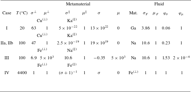
 σ⊥
 σ∥
 σ⊥
 σ∥
 106Ω−1m−1
 μ⊥
 μ∥
 μ⊥
 μ∥
 4π×10−7Hm−1
 TM
 σ
 μ
 φσ
 φμ

 R
 R+e
 e1∈[0,e]
 e1
 e/R∈{0.029;0.257;0.486;0.714}
 n
 n=1
 n=2
 e/R=0.714
 e1/R=0.3
 n=1
 n=2
 |BH|
 |JH|
 Bz
 Jz
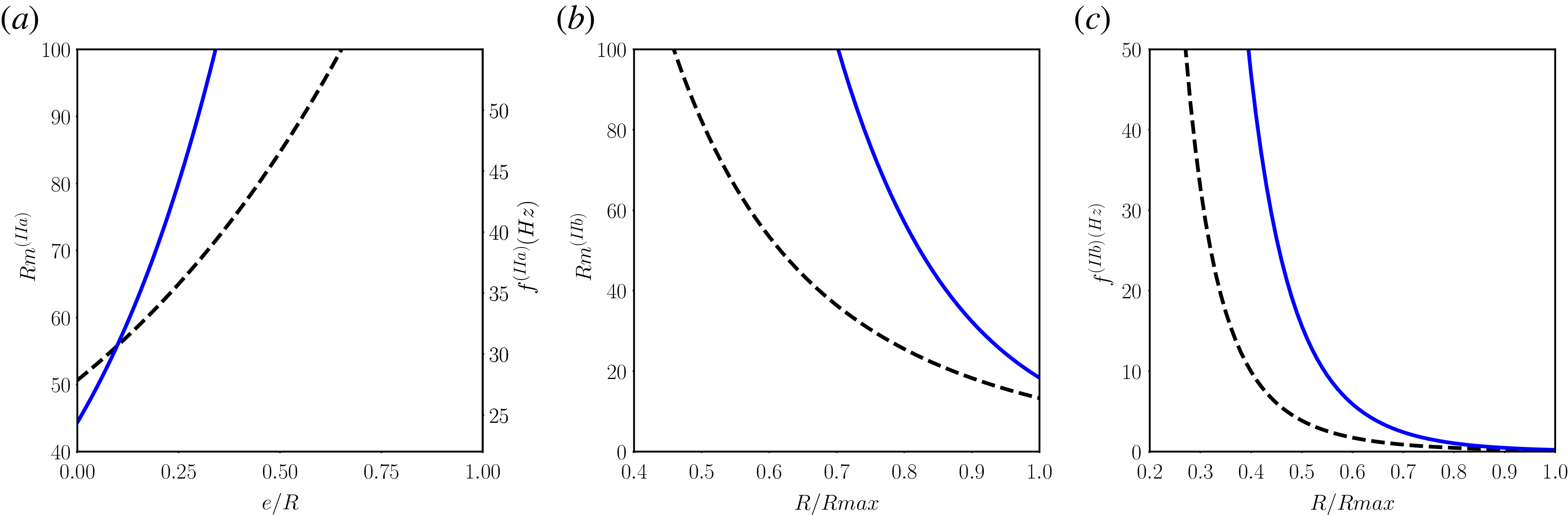
 R
 Rmax
 e/R
 e
 R=7
 n=1
 n=2
 R/Rmax
 Rmax−R
 n=1
 n=2

 e/R=0.5
 e/R=0.3
 n=1
 n=2
 |BH|
 |JH|
 Bz
 Jz

 R
 e
 e/R
 n
 n=1
 n=2
 e/R=0.4
 n=1
 n=2
 |BH|
 |JH|
 Bz
 Jz

 Ω
 σ
 R=1220
 Ω
 Rm(IV)
 e/R
 n=1
 n=2
 e/R
 e/R=0,0.1,0.3,0.5,1
 e/R=0.3
 n=1
 n=2
 |BH|
 |JH|
 Bz
 Jz

 Open access

