1 Introduction
The work of Ingard (Reference Ingard1959) and Myers (Reference Myers1980) on the acoustic boundary condition at an impedance surface in a non-quiescent fluid has formed the basis for most subsequent work, industrial and academic (e.g. Tester Reference Tester1973b ; Koch & Moehring Reference Koch and Moehring1983), where sound attenuation in a moving fluid was important. Over thirty years after the publication of Myers’ paper, and over five years since indisputable evidence was presented, both theoretical (Brambley Reference Brambley2009) and experimental (Renou & Aurégan Reference Renou and Aurégan2011), of its weaknesses, the Ingard–Myers boundary condition continues to be routinely used in aeroacoustics computations to inform engine design.
Inviscid perturbations to a sheared flow over an acoustic liner are governed by the Pridmore-Brown (Reference Pridmore-Brown1958) equation. Modal solutions to this equation show that acoustic liners not only attenuate acoustic modes but also support surface waves – vibrations of the liner and boundary layer – that are not present in the hard-wall case. These waves were classified as surface modes by Rienstra (Reference Rienstra2003), who used uniform flow and the Myers (or Ingard–Myers) model of the impedance lining to find a possible four surface modes per frequency and circumferential order. This work was extended by Brambley (Reference Brambley2013), who accounted for the thin, but non-zero thickness, boundary layer by using the first-order correction terms to the Myers condition (Brambley Reference Brambley2011b ) and found the number of possible surface waves increased to six. At present, no further surface wave solutions to the Pridmore-Brown equation have been identified.
The importance of including a finite-thickness shear layer rather than assuming a uniform slipping flow also manifests in the different convective and absolute stability of the two models. Experimental evidence of an instability in flow over an impedance lining has been reported many times (e.g. Aurégan & Leroux Reference Aurégan and Leroux2008; Marx et al. Reference Marx, Aurégan, Bailliet and Valiére2010). Theoretical predictions of the instability that utilise the Myers model found that in the time domain a numerical instability would grow at the grid scale and swamp any meaningful signal, while in the frequency domain an unstable mode was found with a growth rate unbounded with increasing wavenumber. This was due to the illposedness of the problem of uniform slipping flow over an impedance lining (Brambley Reference Brambley2009). This illposedness is regularised by taking into account a thin but finite-thickness sheared boundary layer, and modified versions of the Myers condition (Myers & Chuang Reference Myers and Chuang1984; Joubert Reference Joubert2010; Brambley Reference Brambley2011b ; Rienstra & Darau Reference Rienstra and Darau2011), correct to first order in the boundary layer thickness, predict convectively or absolutely unstable modes with bounded growth rates.
The accuracy of the current inviscid models was investigated by Gabard (Reference Gabard2013) by considering reflection of acoustic plane waves from an impedance lining in shear flow. It was found that use of the Myers condition can lead to significant errors (of up to
 $14~\text{dB}$
) in predictions of sound attenuation due to the great impact of the boundary layer thickness. Modelling the physics inside the boundary layer more precisely, for instance by expanding to second order in the boundary layer thickness, should therefore lead to more accurate predictions of the absorption and reflection coefficients for an acoustic liner in flow. The accuracy of current boundary conditions and the newly derived conditions are tested in a different way here: by comparing with the exact effective impedance found by numerical solution of the Pridmore-Brown equation; and by comparing the prediction of cut-on and cut-off acoustic modes.
There are a number of common simplifications used in the literature that we follow here, since reasonable agreement is possible between theory using these assumptions and practice (e.g. Boyer, Piot & Brazier Reference Boyer, Piot and Brazier2011). Commonly, acoustic liners are manufactured using a perforated facing sheet having hole diameters and spacings of the order of or larger than a typical boundary layer thickness. The majority of the acoustic lining literature models such linings as homogeneous, however, and here we follow this simplification. When applied in shear flow, the Pridmore-Brown equation possesses a singularity, called the critical layer, wherever the phase speed of a wave is equal to the base flow velocity (that is, when a wave is perfectly convected). It has been shown that the contribution to the resultant sound field of the critical layer is modest at most (Brambley, Darau & Rienstra Reference Brambley, Darau and Rienstra2012). Here we avoid the critical layer in favour of simplicity. Also omitted from the analysis are viscous and nonlinear effects. It has been shown that viscosity alone does not regularise the illposedness of the Myers condition (Brambley Reference Brambley2011a ), but when coupled with a finite-thickness shear layer the problem becomes well posed and the visco-thermal effects allow the unstable mode to restabilise below a critical wavelength (Khamis & Brambley Reference Khamis and Brambley2015) – a phenomenon missing from the inviscid theory. It has also been shown that including viscosity in the boundary layer can be necessary to accurately match theoretical results with experimental data (Renou & Aurégan Reference Renou and Aurégan2010, Reference Renou and Aurégan2011). Nonlinearity with respect to the interaction between sound field, shear flow and liner is beyond the scope of this work.
In this work, new boundary conditions are derived that extend the inviscid theory. In § 2 the governing Pridmore-Brown equations for the acoustic pressure
 $\tilde{p}$
and velocity
 $\tilde{v}$
are stated, and an impedance Ricatti equation is derived for
 $Z(r)=\tilde{p}(r)/\tilde{v}(r)$
. Section 3 describes the asymptotic analysis leading to a boundary condition that is correct to second order in the boundary layer thickness. Section 4 solves the impedance equation by a single fourth-order explicit Runge–Kutta step across the boundary layer; and by a second-order, single-step implicit scheme. Expressions are given for the effective impedance at the lining seen by the acoustics in a plug flow (uniform mean flow). In § 5, the accuracy of each of these models is compared against the Ingard–Myers boundary condition, its first-order correction and numerical simulations. While the second-order boundary condition performs better for thin boundary layers, the single-step implicit Runge–Kutta scheme retains accuracy for high frequencies and short wavelengths, and for thicker boundary layers, making it a viable substitute for the asymptotic boundary conditions outside their regions of validity. In § 6, simplified forms of the conditions are found both for a specific linear shear profile and for the limiting case
 $k/{\it\omega}\gg 1$
satisfied by surface modes. In § 7 it is found that the second-order asymptotic condition is extremely accurate when investigating surface modes and their stability, as well as cut-on and cut-off acoustic modes. The second-order condition does, however, support spurious modes far from its region of asymptotic validity.
2 Governing equations
We are concerned with the dynamics of an inviscid compressible perfect gas, for which (with a star denoting a dimensional variable) the governing equations take the form
 $$\begin{eqnarray}\frac{\partial {\it\rho}^{\ast }}{\partial t^{\ast }}+\boldsymbol{{\rm\nabla}}^{\ast }\boldsymbol{\cdot }({\it\rho}^{\ast }\boldsymbol{u}^{\ast })=0,\quad {\it\rho}\frac{\text{D}\boldsymbol{u}^{\ast }}{\text{D}t^{\ast }}=-\boldsymbol{{\rm\nabla}}^{\ast }p^{\ast },\quad \frac{\text{D}p^{\ast }}{\text{D}t^{\ast }}=c^{\ast 2}\frac{D{\it\rho}^{\ast }}{\text{D}t^{\ast }},\end{eqnarray}$$
where
 $\text{D}/\text{D}t^{\ast }=\partial /\partial t^{\ast }+\boldsymbol{u}^{\ast }\boldsymbol{\cdot }\boldsymbol{{\rm\nabla}}^{\ast }$
is the material derivative,
 ${\it\gamma}=c_{p}^{\ast }/c_{v}^{\ast }$
is the ratio of specific heats, and
 $p^{\ast }$
,
 ${\it\rho}^{\ast }$
and
 $\boldsymbol{u}^{\ast }$
are the fluid pressure, density and velocity, respectively. Equation (2.1c
), relating
 $p^{\ast }$
and
 ${\it\rho}^{\ast }$
, is a consequence of the assumption that the specific entropy remains constant for a given fluid particle (Pierce Reference Pierce1994); for a perfect gas, the speed of sound satisfies
 $c^{\ast 2}={\it\gamma}p^{\ast }/{\it\rho}^{\ast }$
. To non-dimensionalise, we imagine a cylindrical duct
 $(x,r,{\it\theta})$
with an uniform base flow at its centreline, and scale length by the duct radius
 $l^{\ast }$
, density by the centreline value
 ${\it\rho}_{0}^{\ast }$
, velocity by the centreline sound speed
 $c_{0}^{\ast }=\sqrt{{\it\gamma}p_{0}^{\ast }/{\it\rho}_{0}^{\ast }}$
, and pressure by
 ${\it\rho}_{0}^{\ast }c_{0}^{\ast 2}$
. Time is made dimensionless by combining the length and velocity scales,
 $t^{\ast }=l^{\ast }t/c_{0}^{\ast }$
. In such a scheme, the duct radius is unity, and the centreline main-flow density and pressure take the respective values
 ${\it\rho}_{0}=1$
and
 $p_{0}=1/{\it\gamma}$
. The dimensionless centreline velocity is
 $U_{0}=M$
, the centreline Mach number of the flow. In a thin region of width
 ${\it\delta}$
near the acoustically lined duct wall, the steady base flow velocity and density vary, giving
 $r$
-dependent profiles,
 $U(r)$
and
 ${\it\rho}(r)$
. We take the flow to be non-slipping, non-swirling and everywhere parallel, and as such the base pressure is constant across the boundary layer,
 $p\equiv p_{0}$
. The non-dimensional governing equations are, for completeness,
 $$\begin{eqnarray}\frac{\partial {\it\rho}}{\partial t}+\boldsymbol{{\rm\nabla}}\boldsymbol{\cdot }({\it\rho}\boldsymbol{u})=0,\quad {\it\rho}\frac{\text{D}\boldsymbol{u}}{\text{D}t}=-\boldsymbol{{\rm\nabla}}p,\quad \frac{\text{D}p}{\text{D}t}=\frac{{\it\gamma}p}{{\it\rho}}\frac{D{\it\rho}}{\text{D}t}.\end{eqnarray}$$
Small, unsteady perturbations to the base flow are considered, of the form
 $$\begin{eqnarray}q=\tilde{q}(r)\exp \{\text{i}{\it\omega}t-\text{i}kx-\text{i}m{\it\theta}\}.\end{eqnarray}$$
The common exponential factor is omitted henceforth. The velocity and density gradients in the base flow boundary layer alter the effect of the acoustic lining on the acoustics. At the lining, the acoustic pressure drives a wall-normal velocity,
 $\tilde{p}=Z_{b}\tilde{v}$
, for the given impedance of the lining,
 $Z_{b}$
. Governing equations for the acoustic pressure
 $\tilde{p}$
and radial velocity
 $\tilde{v}$
may be derived from (2.2):
 $$\begin{eqnarray}\left(\frac{\tilde{p}^{\prime }}{Q}\right)^{\prime }+\frac{\bar{{\it\alpha}}^{2}}{Q}\tilde{p}=0,\quad \left[\left(\frac{r\tilde{v}}{{\it\omega}-Uk}\right)^{\prime }\frac{Q}{\bar{{\it\alpha}}^{2}}\right]^{\prime }+Q\left(\frac{r\tilde{v}}{{\it\omega}-Uk}\right)=0,\end{eqnarray}$$
where a prime denotes differentiation with respect to
 $r$
, and
 $$\begin{eqnarray}Q(r)=\frac{{\it\rho}({\it\omega}-Uk)^{2}}{r}\quad \text{and}\quad \bar{{\it\alpha}}(r)^{2}={\it\rho}({\it\omega}-Uk)^{2}-k^{2}-\frac{m^{2}}{r^{2}}.\end{eqnarray}$$
It is worth noting that the Pridmore-Brown equation (2.4a
) (Pridmore-Brown Reference Pridmore-Brown1958) and the corresponding equation for the radial velocity (2.4b
) are both second order, in
 $\tilde{p}$
and
 $\tilde{v}$
respectively, with the radial momentum equation stating
 $\tilde{v}\sim \tilde{p}^{\prime }$
. The similarity between the two equations (2.4a,b
) may be highlighted by defining
 ${\it\phi}=r\tilde{v}/({\it\omega}-Uk)$
and rearranging to give
 $$\begin{eqnarray}\frac{Q}{\bar{{\it\alpha}}^{2}}\left(\frac{\tilde{p}^{\prime }}{Q}\right)^{\prime }+\tilde{p}=0,\quad \frac{1}{Q}\left(\frac{Q}{\bar{{\it\alpha}}^{2}}{\it\phi}^{\prime }\right)^{\prime }+{\it\phi}=0.\end{eqnarray}$$
Inherent in the linearisation of the Euler equation, and thus in (2.4a,b
), is the so-called critical layer singularity,
 ${\it\omega}-U(r_{c})k=0$
, where
 $r_{c}$
is the radial location of the critical layer. This occurs when a wave is perfectly convected, and leads to a continuous hydrodynamic spectrum. We neglect the critical layer in this work by assuming that
 $r_{c}$
does not fall within our physical domain.
2.1 The uniform solution
It is well known (see e.g. Vilenksi & Rienstra Reference Vilenksi and Rienstra2007; Brambley & Peake Reference Brambley and Peake2008) that the acoustic pressure and radial velocity in a duct with inviscid uniform flow can be expressed in terms of Bessel functions as
 $\tilde{p}_{u}(r)=E\text{J}_{m}({\it\alpha}r)$
and
 $\tilde{v}_{u}(r)=\text{i}{\it\alpha}E\text{J}_{m}^{\prime }({\it\alpha}r)/({\it\omega}-Mk)$
, where
 ${\it\alpha}^{2}=({\it\omega}-Mk)^{2}-k^{2}$
and
 $E$
is a constant amplitude. Modes for such a flow are found by applying a boundary condition at the lined wall,
 $\tilde{p}_{u}(1)=Z_{eff}\tilde{v}_{u}(1)$
. The effective impedance
 $Z_{eff}$
differs from the true lining impedance
 $Z_{b}$
due to refraction through the sheared boundary layer, which is neglected in the uniform flow model. For example, for the Myers boundary condition,
 $$\begin{eqnarray}Z_{eff}=\frac{{\it\omega}}{{\it\omega}-Mk}Z_{b},\end{eqnarray}$$
where the Doppler factor accounts for refraction across a vortex sheet by enforcing continuity of normal displacement. We would like to choose a
 $Z_{eff}$
such that the easily calculable uniform flow acoustic modes match the modes in the real flow with a sheared boundary layer. Thus,
 $Z_{eff}$
includes information about both the lining impedance
 $Z_{b}$
, and how acoustic modes evolve in shear. This means that solving the uniform flow problem with a lining impedance of
 $Z_{eff}$
is equivalent to solving the true sheared flow problem with the actual lining impedance
 $Z_{b}$
. We are interested in the relationship between
 $Z_{b}$
and
 $Z_{eff}$
.
If we knew both
 ${\it\omega}$
and
 $k$
, then we could find
 $Z_{eff}$
explicitly:
 $$\begin{eqnarray}Z_{eff}=({\it\omega}-Mk)\frac{\text{J}_{m}({\it\alpha})}{\text{i}{\it\alpha}\text{J}_{m}^{\prime }({\it\alpha})}.\end{eqnarray}$$
We do not know both
 $k$
and
 ${\it\omega}$
, a priori, however, and therefore we would like to solve (2.8) for the modes
 $k({\it\omega})$
; a relationship between
 $Z_{eff}$
and the known
 $Z_{b}$
is then needed. For example, the Ingard–Myers boundary condition modelling an infinitely thin shear layer (Eversman & Beckemeyer Reference Eversman and Beckemeyer1972) is given in (2.7), while the first-order asymptotic correction to the Ingard–Myers boundary condition in the limit of a thin shear layer (Brambley Reference Brambley2011b
) is given by
 $$\begin{eqnarray}Z_{eff}=\frac{{\it\omega}}{{\it\omega}-Mk}\,\frac{Z_{b}-\displaystyle \frac{\text{i}({\it\omega}-Mk)^{2}}{{\it\omega}}{\it\delta}I_{0}}{1+\text{i}{\it\omega}Z_{b}\displaystyle \frac{k^{2}+m^{2}}{({\it\omega}-Mk)^{2}}{\it\delta}I_{1}},\end{eqnarray}$$
where
 $I_{0}$
and
 $I_{1}$
are integrals across the thin boundary layer,
 $$\begin{eqnarray}{\it\delta}I_{0}=\int _{0}^{1}\left(1-\frac{({\it\omega}-U(r)k)^{2}{\it\rho}(r)}{({\it\omega}-Mk)^{2}}\right)\text{d}r,\quad {\it\delta}I_{1}=\int _{0}^{1}\left(1-\frac{({\it\omega}-Mk)^{2}}{({\it\omega}-U(r)k)^{2}{\it\rho}(r)}\right)\text{d}r.\end{eqnarray}$$
2.2 An impedance governing equation
Most work concerning acoustic propagation in inviscid fluids begins with equations (2.2) and reduces them to a form of the Pridmore-Brown equation (Pridmore-Brown Reference Pridmore-Brown1958), e.g. equation (2.4a
). Less common is the corresponding governing equation for the radial acoustic velocity
 $\tilde{v}$
, equation (2.4b
). Here, we also work directly with the impedance and derive a new governing equation. We extend the relationship
 $\tilde{p}=Z_{b}\tilde{v}$
at the boundary
 $r=1$
to one valid for all
 $r$
, i.e.
 $Z(r)=\tilde{p}(r)/\tilde{v}(r)$
. The same is done for the uniform flow equivalent, i.e.
 $Z_{u}(r)=\tilde{p}_{u}(r)/\tilde{v}_{u}(r)$
. Hence,
 $Z_{b}\equiv Z(1)$
and
 $Z_{eff}\equiv Z_{u}(1)$
.
From (2.2) and (2.4a,b ) the following relations may be derived:
 $$\begin{eqnarray}\frac{\bar{{\it\alpha}}^{2}}{Q}\tilde{p}=\text{i}\left(\frac{r\tilde{v}}{{\it\omega}-Uk}\right)^{\prime }\quad \text{and}\quad \tilde{p}^{\prime }=-\text{i}Q\left(\frac{r\tilde{v}}{{\it\omega}-Uk}\right).\end{eqnarray}$$
Guided by the form of (2.11), we write
 $$\begin{eqnarray}\frac{1}{r}({\it\omega}-Uk)Z=\frac{\tilde{p}}{~\displaystyle \frac{r\tilde{v}}{({\it\omega}-Uk)}~}.\end{eqnarray}$$
Taking the derivative with respect to
 $r$
and using (2.11) to eliminate
 $\tilde{p}$
and
 $\tilde{v}$
, we find a nonlinear Ricatti equation for
 $Z$
,
 $$\begin{eqnarray}\left[\frac{1}{r}({\it\omega}-Uk)Z\right]^{\prime }=-\text{i}Q+\frac{\text{i}\bar{{\it\alpha}}^{2}}{Q}\left[\frac{1}{r}({\it\omega}-Uk)Z\right]^{2}.\end{eqnarray}$$
Note that (2.13) is a rephrasing of the acoustic equations (2.4a,b
), and thus
 $Z(r)$
represents the lumped impedance of both the boundary and the fluid in
 $[r,1]$
. Since (2.13) is a first-order equation and at the lining the boundary condition gives
 $Z(1)=Z_{b}$
, in the uniform flow region the requirement that
 $Z(r)=Z_{u}(r)$
allows us to find
 $Z_{eff}$
.
The equation (2.13) is exact, and so its numerical solution should correspond with the direct solution of the Pridmore-Brown equation. However, its nonlinearity makes it a less attractive candidate for such computations. Instead we solve (2.13) using two different approximate methods. In § 4, two single-step Runge–Kutta solutions are found, one explicit and one implicit, which exploit the inherently small step size
 ${\it\delta}$
. In appendix B, an alternative asymptotic analysis (to that in § 3) is performed by expanding (2.13) in terms of the small width of the boundary layer,
 ${\it\delta}$
. The two methods vary in essence by where we make our approximations: the first approximately solves an exact equation; the second exactly solves an approximate equation.
3 Deriving the asymptotic solution
In this section the asymptotic boundary condition for the effective impedance is found to second order in
 ${\it\delta}$
by solving (2.4a,b
) inside the boundary layer and matching to the uniform solutions outside the boundary layer.
Outside the boundary layer, the uniform base flow pressure solution may be written
 $\tilde{p}_{u}(r)=E\text{J}_{m}({\it\alpha}r)$
as described above. Expanding this about the lined wall at
 $r=1$
using the boundary layer scaling
 $r=1-{\it\delta}y$
as in Brambley (Reference Brambley2011b
), the outer solution for the pressure becomes
 $$\begin{eqnarray}\tilde{p}_{u}(1-{\it\delta}y)=E\text{J}_{m}({\it\alpha})-{\it\delta}yE{\it\alpha}\text{J}_{m}^{\prime }({\it\alpha})-{\textstyle \frac{1}{2}}{\it\delta}^{2}y^{2}E[{\it\alpha}\text{J}_{m}^{\prime }({\it\alpha})+({\it\alpha}^{2}-m^{2})\text{J}_{m}({\it\alpha})]+O({\it\delta}^{3}).\end{eqnarray}$$
Using the notation
 $p_{\infty }\equiv \tilde{p}_{u}(1)$
, the pressure at the wall
 $r=1$
and
 $v_{\infty }\equiv \tilde{v}_{u}(1)$
, equation (3.1) and the equivalent radial velocity expansion may be written as
 $$\begin{eqnarray}\displaystyle \tilde{p}_{u}(1-{\it\delta}y) & = & \displaystyle p_{\infty }+{\it\delta}y\text{i}({\it\omega}-Mk)v_{\infty }\nonumber\\ \displaystyle & & \displaystyle +\,{\textstyle \frac{1}{2}}{\it\delta}^{2}y^{2}[(k^{2}+m^{2}-({\it\omega}-Mk)^{2})p_{\infty }+\text{i}({\it\omega}-Mk)v_{\infty }]+O({\it\delta}^{3}),\end{eqnarray}$$
 $$\begin{eqnarray}\displaystyle \tilde{v}_{u}(1-{\it\delta}y) & = & \displaystyle v_{\infty }-{\it\delta}y\left(\frac{({\it\omega}-Mk)^{2}-k^{2}-m^{2}}{\text{i}({\it\omega}-Mk)}p_{\infty }-v_{\infty }\right)\nonumber\\ \displaystyle & & \displaystyle +\,\frac{1}{2}{\it\delta}^{2}y^{2}\left[\frac{3m^{2}+k^{2}-({\it\omega}-Mk)^{2}}{\text{i}({\it\omega}-Mk)}p_{\infty }+(2+k^{2}+m^{2}-({\it\omega}-Mk)^{2})v_{\infty }\right]\nonumber\\ \displaystyle & & \displaystyle +\,O({\it\delta}^{3}).\end{eqnarray}$$
 $y\rightarrow \infty$
.
In terms of the boundary layer variable
 $y$
, equations (2.4a,b
) become
 $$\begin{eqnarray}\left(\frac{\tilde{p}_{y}}{{\it\rho}({\it\omega}-Uk)^{2}}\right)_{y}={\it\delta}\left(\frac{y\tilde{p}_{y}}{{\it\rho}({\it\omega}-Uk)^{2}}\right)_{y}-{\it\delta}^{2}\left(1-\frac{k^{2}+m^{2}}{{\it\rho}({\it\omega}-Uk)^{2}}\right)\tilde{p}+O({\it\delta}^{3})\end{eqnarray}$$
for the pressure, and
 $$\begin{eqnarray}\displaystyle & & \displaystyle \left[\left(\frac{\tilde{v}}{{\it\omega}-Uk}\right)_{y}\frac{{\it\rho}({\it\omega}-Uk)^{2}}{{\it\rho}({\it\omega}-Uk)^{2}-k^{2}-m^{2}}\right]_{y}={\it\delta}\left(\frac{\tilde{v}}{{\it\omega}-Uk}\frac{{\it\rho}({\it\omega}-Uk)^{2}}{{\it\rho}({\it\omega}-Uk)^{2}-k^{2}-m^{2}}\right)_{y}\nonumber\\ \displaystyle & & \displaystyle \quad -\,{\it\delta}\left[\left(\frac{\tilde{v}}{{\it\omega}-Uk}\right)_{y}\frac{2m^{2}y{\it\rho}({\it\omega}-Uk)^{2}}{[{\it\rho}({\it\omega}-Uk)^{2}-k^{2}-m^{2}]^{2}}\right]_{y}-{\it\delta}^{2}\left(\frac{\tilde{v}}{{\it\omega}-Uk}\,{\it\rho}({\it\omega}-Uk)^{2}\right)\nonumber\\ \displaystyle & & \displaystyle \quad +\,{\it\delta}^{2}\left(\frac{\tilde{v}}{{\it\omega}-Uk}\frac{y{\it\rho}({\it\omega}-Uk)^{2}}{[{\it\rho}({\it\omega}-Uk)^{2}-k^{2}-m^{2}]^{2}}({\it\rho}({\it\omega}-Uk)^{2}+m^{2}-k^{2})\right)_{y}\nonumber\\ \displaystyle & & \displaystyle \quad -\,{\it\delta}^{2}\left[\left(\frac{\tilde{v}}{{\it\omega}-Uk}\right)_{y}\frac{4m^{2}y^{2}{\it\rho}({\it\omega}-Uk)^{2}}{[{\it\rho}({\it\omega}-Uk)^{2}-k^{2}-m^{2}]^{3}}({\it\rho}({\it\omega}-Uk)^{2}-k^{2})\right]_{y}+O({\it\delta}^{3})\end{eqnarray}$$
for the radial velocity. Here
 ${\it\rho}$
and
 $U$
are now the corresponding base density and axial velocity as functions of
 $y$
. A subscript denotes differentiation.
Solving (3.3) and (3.4) to second order produces the inner solutions (see appendix A for details). When evaluated at the wall, the second-order correction to the
 $\tilde{v}$
expansion is singular if
 $({\it\omega}-Mk)^{2}=k^{2}+m^{2}$
. Solutions of the Pridmore-Brown equation exist at this point. Thus, the singularity is a consequence of the asymptotic expansion and is spurious. Close to the new singular point, one could simply revert to using the first-order expansion as derived by Brambley (Reference Brambley2011b
), which is unaffected by the unphysical singularity.
Matching with the outer solutions (3.2) and evaluating at the boundary
 $y=0$
gives, after some algebra,
 $$\begin{eqnarray}\displaystyle \tilde{p}(0) & = & \displaystyle \tilde{p}_{u}(0)+\text{i}({\it\omega}-Mk)\tilde{v}_{u}(0){\it\delta}I_{0}+\text{i}({\it\omega}-Mk)\tilde{v}_{u}(0){\it\delta}^{2}I_{2}\nonumber\\ \displaystyle & & \displaystyle +\,(k^{2}+m^{2})\tilde{p}_{u}(0)({\it\delta}I_{0}{\it\delta}I_{1}-{\it\delta}^{2}I_{3})-({\it\omega}-Mk)^{2}\tilde{p}_{u}(0){\it\delta}^{2}I_{7}+O({\it\delta}^{3}),\end{eqnarray}$$
 $$\begin{eqnarray}\displaystyle \tilde{v}(0) & = & \displaystyle \frac{{\it\omega}}{{\it\omega}-Mk}\left\{\tilde{v}_{u}(0)-\text{i}\tilde{p}_{u}(0)\frac{k^{2}+m^{2}}{{\it\omega}-Mk}{\it\delta}I_{1}+({\it\omega}-Mk)^{2}\tilde{v}_{u}(0){\it\delta}^{2}I_{2}\right.\nonumber\\ \displaystyle & & \displaystyle +\,(k^{2}+m^{2})\tilde{v}_{u}(0){\it\delta}^{2}I_{3}+\text{i}\tilde{p}_{u}(0)\frac{k^{2}+m^{2}}{{\it\omega}-Mk}\frac{k^{2}-m^{2}-({\it\omega}-Mk)^{2}}{k^{2}+m^{2}-({\it\omega}-Mk)^{2}}{\it\delta}^{2}I_{3}\nonumber\\ \displaystyle & & \displaystyle +\,(k^{2}+m^{2})\tilde{v}_{u}(0)({\it\delta}I_{0}{\it\delta}I_{1}-{\it\delta}^{2}I_{2}-{\it\delta}^{2}I_{5})\nonumber\\ \displaystyle & & \displaystyle \left.+\,\frac{2\text{i}m^{2}\tilde{p}_{u}(0)}{{\it\omega}-Mk}\left(\frac{k^{2}+m^{2}}{k^{2}+m^{2}-({\it\omega}-Mk)^{2}}{\it\delta}^{2}I_{6}-{\it\delta}^{2}I_{4}\right)\right\}+O({\it\delta}^{3}),\end{eqnarray}$$
 $I_{j}$
are
 $$\begin{eqnarray}\left.\begin{array}{@{}c@{}}\displaystyle I_{0}=\int _{0}^{\infty }{\it\chi}_{0}(y)\,\text{d}y,\quad I_{1}=\int _{0}^{\infty }{\it\chi}_{1}(y)\,\text{d}y,\quad I_{2}=\int _{0}^{\infty }y{\it\chi}_{0}(y)\,\text{d}y,\\ \displaystyle I_{3}=\int _{0}^{\infty }y{\it\chi}_{1}(y)\,\text{d}y,\quad I_{4}=\int _{0}^{\infty }y{\it\chi}_{2}(y)\,\text{d}y,\quad I_{5}=\int _{0}^{\infty }{\it\chi}_{1}(y)\int _{0}^{y}{\it\chi}_{0}(y^{\prime })\,\text{d}y^{\prime }\,\text{d}y,\\ \displaystyle I_{6}=\int _{0}^{\infty }y{\it\chi}_{1}(y){\it\chi}_{2}(y)\,\text{d}y,\quad I_{7}=\int _{0}^{\infty }{\it\chi}_{0}(y)\int _{0}^{y}\left(1-\frac{k^{2}+m^{2}}{{\it\rho}(y^{\prime })({\it\omega}-U(y^{\prime })k)^{2}}\right)\text{d}y^{\prime }\,\text{d}y,\end{array}\right\}\end{eqnarray}$$
with
 $$\begin{eqnarray}\left.\begin{array}{@{}c@{}}\displaystyle {\it\chi}_{0}(y)=\left[1-\frac{{\it\rho}({\it\omega}-Uk)^{2}}{({\it\omega}-Mk)^{2}}\right],\quad {\it\chi}_{1}(y)=\left[1-\frac{({\it\omega}-Mk)^{2}}{{\it\rho}({\it\omega}-Uk)^{2}}\right],\\ \displaystyle {\it\chi}_{2}(y)=\left[1-\frac{({\it\omega}-Mk)^{2}-k^{2}-m^{2}}{{\it\rho}({\it\omega}-Uk)^{2}-k^{2}-m^{2}}\right].\end{array}\right\}\end{eqnarray}$$
The impedance of the boundary is the ratio of the acoustic pressure to the normal velocity that it drives, so we write
 $Z_{b}=\tilde{p}(0)/\tilde{v}(0)$
using (3.5). We identify the effective impedance with the same ratio for the uniform flow variables:
 $Z_{eff}=p_{\infty }/v_{\infty }$
. Using these two relationships, we may rearrange the ratio of (3.5a
) and (3.5b
) to find an expression for the effective impedance of an acoustic liner with an inviscid sheared boundary layer:
 $$\begin{eqnarray}Z_{eff}=\frac{{\it\omega}}{{\it\Omega}_{u}}\frac{\displaystyle Z_{b}-\frac{\text{i}{\it\Omega}_{u}^{2}}{{\it\omega}}({\it\delta}I_{0}+{\it\delta}^{2}I_{2})-Z_{b}{\it\mu}^{2}{\it\delta}^{2}I_{2}+{\it\sigma}_{+}Z_{b}({\it\delta}I_{0}{\it\delta}I_{1}+{\it\delta}^{2}I_{3}-{\it\delta}^{2}I_{5})}{\displaystyle 1+\text{i}{\it\sigma}_{+}\frac{{\it\omega}Z_{b}}{{\it\Omega}_{u}^{2}}{\it\delta}I_{1}+{\it\Upsilon}_{1}{\it\delta}^{2}I_{3}+{\it\Upsilon}_{2}\left({\it\delta}^{2}I_{4}-\frac{{\it\sigma}_{+}}{{\it\mu}^{2}}{\it\delta}^{2}I_{6}\right)+{\it\sigma}_{+}{\it\delta}I_{0}{\it\delta}I_{1}-{\it\Omega}_{u}^{2}{\it\delta}^{2}I_{7}}+O({\it\delta}^{3}),\end{eqnarray}$$
where
 ${\it\sigma}_{+}=k^{2}+m^{2}$
,
 ${\it\Omega}_{u}={\it\omega}-Mk$
and
 ${\it\mu}^{2}={\it\sigma}_{+}-{\it\Omega}_{u}^{2}$
, and where
 $$\begin{eqnarray}\displaystyle {\it\Upsilon}_{1}=\frac{\text{i}{\it\sigma}_{+}{\it\omega}Z_{b}}{{\it\Omega}_{u}^{2}}\left(\frac{2m^{2}}{{\it\mu}^{2}}-1\right)-{\it\sigma}_{+},\quad {\it\Upsilon}_{2}=2\text{i}m^{2}\frac{{\it\omega}Z_{b}}{{\it\Omega}_{u}^{2}}. & & \displaystyle\end{eqnarray}$$
Equation (3.8) readily reduces to the modified boundary condition as derived by Brambley (Reference Brambley2011b
) at
 $O({\it\delta})$
, equation (2.9), and to the classical Myers condition (2.7) in the limit
 ${\it\delta}\rightarrow 0$
. Figure 1 shows that the condition is correct to the stated asymptotic order.
The relative errors of the leading (black dotted), first (blue dashed) and second (red solid) orders of the new boundary condition (3.8) when compared with numerical solutions of the Pridmore-Brown equation. The green dash-dotted lines have gradients of 1, 2 and 3 beginning from the top and moving down. Parameters used are
 $k=\pm 1\pm \text{i},\pm \text{i}$
and
 ${\it\omega}=1$
,
 $m=0$
,
 $M=0.5$
with the tanh boundary layer profile of (5.1). Relative error is defined by
 $|Z^{\ast }/Z_{eff}-1|$
, where
 $Z^{\ast }$
is the approximation from the specified model, and
 $Z_{eff}$
is the exact result from (2.8).

Equation (3.8) may be applied in the physical
 $r$
domain by transforming the integrals
 $I_{j}$
as follows:
 $$\begin{eqnarray}\left.\begin{array}{@{}c@{}}\displaystyle {\it\delta}I_{0}=\int _{0}^{1}{\it\chi}_{0}(r)\,\text{d}r,\quad {\it\delta}I_{1}=\int _{0}^{1}{\it\chi}_{1}(r)\,\text{d}r,\quad {\it\delta}^{2}I_{2}=\int _{0}^{1}(1-r){\it\chi}_{0}(r)\,\text{d}r,\\ \displaystyle {\it\delta}^{2}I_{3}=\int _{0}^{1}(1-r){\it\chi}_{1}(r)\,\text{d}r,\quad {\it\delta}^{2}I_{4}=\int _{0}^{1}(1-r){\it\chi}_{2}(r)\,\text{d}r,\\ \displaystyle {\it\delta}^{2}I_{5}=\int _{0}^{1}{\it\chi}_{1}(r)\int _{r}^{1}{\it\chi}_{0}(r^{\prime })\,\text{d}r^{\prime }\,\text{d}r,\quad {\it\delta}^{2}I_{6}=\int _{0}^{1}(1-r){\it\chi}_{1}(r){\it\chi}_{2}(r)\,\text{d}r,\\ \displaystyle {\it\delta}^{2}I_{7}=\int _{0}^{1}{\it\chi}_{0}(r)\int _{r}^{1}\left(1-\frac{{\it\sigma}_{+}}{{\it\rho}(r^{\prime }){\it\Omega}(r^{\prime })^{2}}\right)\text{d}r^{\prime }\,\text{d}r.\end{array}\right\}\end{eqnarray}$$
An example of the accuracy of this boundary condition is given in § 5, and an explicit form for a linear boundary layer profile is given in § 6.1.
4 The Runge–Kutta solutions
Here we derive an expression for
 $Z_{eff}$
by approximately solving (2.13) using a single step of a fourth-order explicit Runge–Kutta method (see Hairer, Nørsett & Wanner Reference Hairer, Nørsett and Wanner1993), and a second-order, single-step implicit scheme.
Equation (2.13) may be transformed as follows. Dividing (2.13) through by
 $({\it\omega}-Mk)^{2}$
produces
 $$\begin{eqnarray}\frac{1}{{\it\omega}-Mk}L^{\prime }=-\text{i}\tilde{Q}+\frac{\text{i}\bar{{\it\alpha}}^{2}}{\tilde{Q}({\it\omega}-Mk)^{2}}L^{2},\end{eqnarray}$$
where
 $\tilde{Q}=Q/({\it\omega}-Mk)^{2}$
, an
 $O(1)$
quantity for all
 ${\it\omega}$
,
 $k$
, and
 $$\begin{eqnarray}L=\frac{({\it\omega}-Uk)}{r({\it\omega}-Mk)}Z.\end{eqnarray}$$
The quantity
 $L$
may be split into a uniform flow value,
 $L_{u}=Z_{u}/r$
, and a perturbation due to the presence of the boundary layer,
 $\tilde{L}$
, such that
 $$\begin{eqnarray}L=L_{u}+\tilde{L}.\end{eqnarray}$$
Equation (4.1) has the associated data
 $L_{u}(1)=Z_{eff}$
, and
 $L=L_{u}$
outside the boundary layer. For a uniform flow of Mach number
 $M$
and constant density
 ${\it\rho}\equiv 1$
, (4.1) reduces to
 $$\begin{eqnarray}\frac{1}{({\it\omega}-Mk)}L_{u}^{\prime }=-\frac{\text{i}}{r}+\text{i}r\left(1-\frac{\displaystyle k^{2}+\frac{m^{2}}{r^{2}}}{({\it\omega}-Mk)^{2}}\right)L_{u}^{2}.\end{eqnarray}$$
Equation (4.4) may then be used in (4.1) along with the decomposition (4.3) to form a governing equation for
 $\tilde{L}(r)$
:
 $$\begin{eqnarray}\displaystyle \frac{1}{({\it\omega}-Mk)}\tilde{L}^{\prime } & = & \displaystyle \frac{\text{i}}{r}\left[1-\frac{{\it\rho}({\it\omega}-Uk)^{2}}{({\it\omega}-Mk)^{2}}\right]+\text{i}r\frac{\displaystyle k^{2}+\frac{m^{2}}{r^{2}}}{({\it\omega}-Mk)^{2}}\left[1-\frac{({\it\omega}-Mk)^{2}}{{\it\rho}({\it\omega}-Uk)^{2}}\right]L_{u}^{2}\nonumber\\ \displaystyle & & \displaystyle +\,\text{i}r\left[1-\frac{\displaystyle k^{2}+\frac{m^{2}}{r^{2}}}{{\it\rho}({\it\omega}-Uk)^{2}}\right](2L_{u}\tilde{L}+\tilde{L}^{2}).\end{eqnarray}$$
The asymptotics of (4.5) may be found in appendix B, where it is shown that the modified Myers (Brambley Reference Brambley2011b ) condition may be cleanly reproduced from (4.5) but the second-order extension runs into difficulties concerning non-uniqueness. Here, we proceed with approximate solutions to (4.5).
4.1 The explicit scheme
In order to ensure the correct
 ${\it\delta}\rightarrow 0$
behaviour, we use the decomposition (4.3) and solve (4.5) for
 $\tilde{L}(r)$
, with the necessary condition that
 $\tilde{L}=0$
in uniform flow (for
 $r<1-{\it\delta}$
). While this is technically only valid for profiles with
 $U\equiv M$
for
 $r<1-{\it\delta}$
, for a
 $99\,\%\,U_{0}$
boundary layer thickness the approximation
 $\tilde{L}=0$
for
 $r<1-{\it\delta}$
is a reasonable one. We choose to step from the top of the boundary layer at
 $r=1-{\it\delta}$
, with the initial condition
 $\tilde{L}(1-{\it\delta})=0$
, to the lining at
 $r=1$
, where the boundary condition
 $\tilde{L}(1)={\it\omega}Z_{b}/({\it\omega}-Mk)-Z_{eff}$
gives
 $Z_{eff}$
as a function of
 $Z_{b}$
. Using the analytic uniform solution defined in § 2.1, we can treat as known the intermediate values of
 $L_{u}(r)$
that arise.
To perform the step, we define the fourth-order explicit Runge–Kutta difference equation
 $\tilde{L}_{1}=\tilde{L}_{0}+{\it\delta}/6(k_{1}+2k_{2}+2k_{3}+k_{4})$
, where
 $\tilde{L}_{0}=\tilde{L}(1-{\it\delta})=0$
. Defining
 $$\begin{eqnarray}A=\frac{\text{i}({\it\omega}-Mk)}{r}{\it\chi}_{0},\quad B=\text{i}r\frac{k^{2}+m^{2}/r^{2}}{{\it\omega}-Mk}{\it\chi}_{1},\quad C=\text{i}r({\it\omega}-Mk)\left[1-\frac{k^{2}+m^{2}/r^{2}}{{\it\rho}({\it\omega}-Uk)^{2}}\right],\end{eqnarray}$$
with
 ${\it\chi}_{j}$
defined as in (3.7), the
 $k_{j}$
terms become
 $$\begin{eqnarray}\displaystyle & \displaystyle k_{1}=A(1-{\it\delta})+B(1-{\it\delta})L_{u}(1-{\it\delta})^{2}, & \displaystyle\end{eqnarray}$$
 $$\begin{eqnarray}\displaystyle & \displaystyle k_{2}=A(1-{\it\delta}/2)+B(1-{\it\delta}/2)L_{u}(1-{\it\delta}/2)^{2}+C(1-{\it\delta}/2)\left(2L_{u}(1-{\it\delta}/2)\frac{{\it\delta}}{2}k_{1}+\frac{{\it\delta}^{2}}{4}k_{1}^{2}\right), & \displaystyle \nonumber\\ \displaystyle & & \displaystyle\end{eqnarray}$$
 $$\begin{eqnarray}\displaystyle & \displaystyle k_{3}=A(1-{\it\delta}/2)+B(1-{\it\delta}/2)L_{u}(1-{\it\delta}/2)^{2}+C(1-{\it\delta}/2)\left(2L_{u}(1-{\it\delta}/2)\frac{{\it\delta}}{2}k_{2}+\frac{{\it\delta}^{2}}{4}k_{2}^{2}\right), & \displaystyle \nonumber\\ \displaystyle & & \displaystyle\end{eqnarray}$$
 $$\begin{eqnarray}\displaystyle & \displaystyle k_{4}=A(1)+B(1)Z_{eff}^{2}+C(1)(2Z_{eff}{\it\delta}k_{3}+{\it\delta}^{2}k_{3}^{2}). & \displaystyle\end{eqnarray}$$
 $r=1$
, giving
 $$\begin{eqnarray}Z_{eff}=\frac{{\it\omega}}{{\it\omega}-Mk}Z_{b}-\frac{{\it\delta}}{6}(k_{1}+2k_{2}+2k_{3}+k_{4}).\end{eqnarray}$$
If we extract the
 $Z_{eff}$
from
 $k_{4}$
, defining
 $k_{4}=\tilde{k}_{4}+[B(1)Z_{eff}+2C(1){\it\delta}k_{3}]Z_{eff}$
, where
 $\tilde{k}_{4}=A(1)+{\it\delta}^{2}C(1)k_{3}^{2}$
, we can rearrange (4.8) to find
 $$\begin{eqnarray}Z_{eff}=\frac{{\it\omega}}{{\it\omega}-Mk}\frac{\displaystyle Z_{b}-\frac{{\it\delta}}{6}(1-Mk/{\it\omega})(k_{1}+2k_{2}+2k_{3}+\tilde{k}_{4})}{\displaystyle 1+\frac{{\it\delta}}{6}(B(1)Z_{eff}+2{\it\delta}C(1)k_{3})},\end{eqnarray}$$
which then gives
 $Z_{eff}$
as a function of
 $Z_{b}$
. The classical Myers condition is recovered in the limit
 ${\it\delta}\rightarrow 0$
, as we would hope (Eversman & Beckemeyer Reference Eversman and Beckemeyer1972; Tester Reference Tester1973a
). The form of (4.9) bears a striking resemblance to that of the modified Myers condition.
4.2 A single-step implicit scheme
Here we define a trapezoidal second-order, single-step implicit Runge–Kutta scheme and use it for a single step to approximate
 $Z_{eff}$
. For this scheme, the fundamental difference equation for the differential equation
 $y^{\prime }=f(x,y)$
is
 $$\begin{eqnarray}y_{n+1}=y_{n}+\frac{h}{2}(f(x_{n},y_{n})+f(x_{n+1},y_{n+1})).\end{eqnarray}$$
The method is implicit due to the appearance of
 $y_{n+1}$
on both sides of (4.10).
We use the scheme to first step back from the boundary, which has a known impedance
 $Z_{b}$
, through the sheared boundary layer profile to the edge of the boundary layer at
 $r=1-{\it\delta}$
; and then to step forward from
 $r=1-{\it\delta}$
to
 $r=1$
assuming a uniform flow. The details of these steps are found in appendix D.
The method results in the effective impedance
 $$\begin{eqnarray}Z_{eff}=X_{1}+{\textstyle \frac{1}{2}}{\it\delta}(\tilde{k}_{1}+\tilde{k}_{2}),\end{eqnarray}$$
where
 $$\begin{eqnarray}X_{1}=X_{0}-\frac{1}{2}{\it\delta}(k_{1}+k_{2})\quad \text{and}\quad X_{0}=\frac{{\it\omega}}{{\it\omega}-Mk}Z_{b},\end{eqnarray}$$
with
 $$\begin{eqnarray}\displaystyle k_{1}=A_{1}(1)+B_{1}(1)X_{0}^{2}, & & \displaystyle\end{eqnarray}$$
 $$\begin{eqnarray}\displaystyle k_{2} & = & \displaystyle \left(\frac{2}{{\it\delta}^{2}B_{1}(1-{\it\delta})}+2\frac{X_{0}}{{\it\delta}}-k_{1}\right)\nonumber\\ \displaystyle & & \displaystyle \times \,\left(1-\left\{1-\frac{4A_{1}(1-{\it\delta})/B_{1}(1-{\it\delta})+(2X_{0}-{\it\delta}k_{1})^{2}}{\displaystyle \left(\frac{2}{{\it\delta}B_{1}(1-{\it\delta})}+2X_{0}-{\it\delta}k_{1}\right)^{2}}\right\}^{1/2}\right),\end{eqnarray}$$
for
 $$\begin{eqnarray}\displaystyle A_{1}(r)=-\frac{\text{i}}{r}\frac{{\it\rho}({\it\omega}-Uk)^{2}}{{\it\omega}-Mk},\quad B_{1}(r)=\text{i}r({\it\omega}-Mk)\left(1-\frac{k^{2}+m^{2}/r^{2}}{{\it\rho}({\it\omega}-Uk)^{2}}\right), & & \displaystyle\end{eqnarray}$$
and with
 $$\begin{eqnarray}\displaystyle & \displaystyle \tilde{k}_{1}=A_{2}(1-{\it\delta})+B_{2}(1-{\it\delta})X_{1}^{2}, & \displaystyle\end{eqnarray}$$
 $$\begin{eqnarray}\displaystyle & \displaystyle \tilde{k}_{2}=\left(\frac{2}{{\it\delta}^{2}B_{2}(1)}-2\frac{X_{1}}{{\it\delta}}-\tilde{k}_{1}\right)\left(1-\left\{1-\frac{4A_{2}(1)/B_{2}(1)+(2X_{1}+{\it\delta}\tilde{k}_{1})^{2}}{\displaystyle \left(\frac{2}{{\it\delta}B_{2}(1)}-2X_{1}-{\it\delta}\tilde{k}_{1}\right)^{2}}\right\}^{1/2}\right), & \displaystyle\end{eqnarray}$$
 $$\begin{eqnarray}\displaystyle A_{2}(r)=-\frac{\text{i}}{r}({\it\omega}-Mk),\quad B_{2}(r)=\text{i}r({\it\omega}-Mk)\left(1-\frac{k^{2}+m^{2}/r^{2}}{({\it\omega}-Mk)^{2}}\right). & & \displaystyle\end{eqnarray}$$
The two steps used here (back then forward) allow the resulting condition to be a direct map from
 $Z_{b}$
to
 $Z_{eff}$
(like the asymptotic boundary condition (3.8)), without intermediate values of
 $Z_{u}$
having to be used (as in the explicit Runge–Kutta scheme (4.9)).
5 Accuracy of models of
 $Z_{eff}$

To measure the accuracy of the boundary conditions derived above, numerical solutions of the full Pridmore-Brown equation were found. This was achieved using a sixth-order finite difference discretisation on a computational grid spaced uniformly in
 ${\it\xi}$
, where
 $r=\tanh (A{\it\xi})/\tanh (A)$
, and
 $A$
is a stretching parameter, in order to cluster points near
 $r=1$
to resolve the boundary layer. Regularity conditions were imposed at
 $r=0$
, and the wall boundary condition was
 $\tilde{p}(1)=1$
, with
 $\tilde{v}$
free. Roots of the dispersion relation
 $Z_{b}=\tilde{p}/\tilde{v}$
were found via Newton–Raphson iteration over
 $k$
. The tanh velocity profile (Rienstra & Vilenski Reference Rienstra and Vilenski2008)
 $$\begin{eqnarray}\displaystyle U(r)=M\tanh \left(\frac{1-r}{{\it\delta}}\right)+M(1-\tanh (1/{\it\delta}))\left(\frac{1+\tanh (1/{\it\delta})}{{\it\delta}}r+(1+r)\right)(1-r), & & \displaystyle \nonumber\\ \displaystyle & & \displaystyle\end{eqnarray}$$
was used to generate the following results, with a constant density
 ${\it\rho}(r)\equiv 1$
. This base flow has a displacement thickness
 $$\begin{eqnarray}{\it\delta}^{\ast }=\frac{1}{6{\it\delta}}(\tanh ^{2}(1/{\it\delta})-1)+\frac{1}{3}(1+2\tanh (1/{\it\delta}))-{\it\delta}\ln (\cosh (1/{\it\delta})),\end{eqnarray}$$
which for
 ${\it\delta}\in (10^{-7},10^{-1})$
gives
 ${\it\delta}^{\ast }/{\it\delta}=0.69$
to two decimal places.
A good initial test of the boundary conditions, and one which seems to be missing from the literature concerning such impedance boundary conditions, is to directly check how well the effective impedance is approximated. By solving the Pridmore-Brown equation throughout the complex
 $k$
-plane for a given
 ${\it\omega}$
and
 $m$
, a boundary impedance
 $Z_{b}$
is generated at each
 $k$
. This solution has a unique uniform flow equivalent and the value of
 $Z_{u}(1)$
of this uniform flow mode, from (2.8), is the
 $Z_{eff}$
against which we test the models.
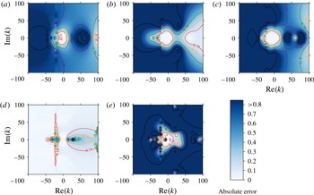
Absolute errors in the complex
 $k$
-plane of the predicted
 $Z_{eff}$
for each boundary condition. The colour scheme is normalised such that the darkest blue is an error greater than or equal to 1.5 times the mean Myers error. The red contour surrounds errors lower than the lowest quartile of the five plotted data sets combined. Shown are (a) the Myers condition (2.7), (b) the modified Myers condition (2.9), (c) the second-order
 $O({\it\delta}^{2})$
asymptotic condition (3.8), (d) the single-step implicit Runge–Kutta condition (4.11) and (e) the explicit Runge–Kutta condition (4.9). The error was calculated as
 $\min \{|Z_{1}-Z_{2}|,|1/Z_{1}-1/Z_{2}|\}$
. Parameters are
 ${\it\omega}=31$
,
 $m=24$
,
 $M=0.5$
,
 ${\it\delta}=2\times 10^{-3}$
, for a tanh velocity profile (5.1) and constant base density
 ${\it\rho}(r)\equiv 1$
. The boundary impedance at each point is found from the numerical solution of the Pridmore-Brown equation, (2.4a
).

Figure 2 shows the absolute errors in the complex
 $k$
-plane of the predicted
 $Z_{eff}$
for each boundary condition. For the thin boundary layer thickness
 ${\it\delta}=2\times 10^{-3}$
, the asymptotic conditions perform well. As one would expect, the
 $O({\it\delta}^{2})$
asymptotic solution, figure 2(c), is more accurate throughout the plotted domain than the modified Myers condition, figure 2(b), which in turn is more accurate than the Myers condition, figure 2(a). For the parameters
 ${\it\omega}=31$
and
 $m=24$
(typical values for rotor-alone noise in an aeroengine bypass duct at take-off (McAlpine et al.
Reference McAlpine, Astley, Hii, Baker and Kempton2006)), and the restriction to
 $\text{Im}(k),\text{Re}(k)\in [-100,100]$
, we are well within the region of asymptotic validity,
 ${\it\omega},m,k\ll 1/{\it\delta}$
. The single-step explicit Runge–Kutta scheme, figure 2(e), performs well in regions where the scheme is stable, but blows up erratically due to the stiffness of the impedance Ricatti equation (2.13). The single-step implicit scheme, figure 2(d), is reasonably accurate for most of the domain, but has regions where the error is large. Sudden changes inside the boundary layer are not modelled well by the implicit scheme, which utilises data points only at either side of the layer; this suggests that the implicit scheme is not suitable for predicting surface modes, and may explain the loss of accuracy of the implicit scheme in the darker regions of figure 2(d). The Myers condition, figure 2(a), also loses accuracy in these regions due to its vanishingly thin shear layer. The well-posed asymptotic schemes in figure 2(b,c) do not have this problem: the bulk treatment of the shear as integrals across the boundary layer, equation (3.6), allow better modelling of variations inside the boundary layer.


In the bypass duct of an aeroengine, the boundary layer may be much thicker than
 $10^{-3}$
. Figure 3 shows results for
 ${\it\delta}=3\times 10^{-2}$
, with all other parameters as in figure 2. For this relatively thick boundary layer, the region of asymptotic validity is
 $k\ll 33$
, so it is no surprise that the breakdown of the asymptotic models (figure 3
b,c) occurs within the plotted domain. The Myers condition, figure 3(a), is also only usefully accurate in a small region near the origin. The instability of the explicit method makes it unusable in most circumstances (figure 3
e). The A-stable single-step implicit scheme, however, comes into its own for thicker boundary layers. Figure 3(d) shows the implicit scheme to be extremely accurate throughout the
 $k$
domain. Importantly, the accuracy is not lessened as
 $k$
increases past
 $1/{\it\delta}$
, meaning that the single-step implicit scheme may also be useful when short-wavelength, high-frequency waves interact with a thick boundary layer. There are, however, larger errors near the Doppler-shifted origin, which is a region important for modes close to cut-on. These errors can manifest as erroneous instabilities of the least cut-off upstream modes, discussed in § 7.
6 Simplified forms and limiting cases
Although expressible analytically, the boundary condition in (3.8) contains integrals across the boundary layer that for a general boundary layer profile must be performed numerically. The single-step implicit scheme boundary condition (4.11) is also complicated in its most general form. We now investigate specific situations when fully closed, simplified forms of the conditions may be found.
6.1 Linear boundary profile
In the case of a linear boundary layer velocity profile,
 $$\begin{eqnarray}U(r)=\left\{\begin{array}{@{}ll@{}}M(1-r)/{\it\delta}, & (1-r)<{\it\delta},\\ M, & (1-r)>{\it\delta},\end{array}\right.\end{eqnarray}$$
with a constant density
 ${\it\rho}\equiv 1$
, the integrals
 $I_{j}$
in (3.8) may be performed analytically and a closed-form expression for the
 $O({\it\delta}^{2})$
asymptotic solution can be written:
 $$\begin{eqnarray}Z_{eff}=\frac{{\it\omega}}{{\it\omega}-Mk}\frac{\displaystyle Z_{b}+{\it\delta}\frac{\text{i}Mk}{3{\it\omega}}(3{\it\omega}-2Mk)+{\it\delta}^{2}\frac{Mk}{12{\it\omega}}(8Z_{b}(k^{2}+m^{2})-({\it\omega}Z_{b}-\text{i})(4{\it\omega}-3kM))}{\displaystyle 1+\text{i}{\it\delta}MkZ_{b}\frac{(k^{2}+m^{2})}{({\it\omega}-Mk)^{2}}+{\it\delta}^{2}{\it\Upsilon}_{3}},\end{eqnarray}$$
where
 $$\begin{eqnarray}\displaystyle {\it\Upsilon}_{3} & = & \displaystyle \frac{Mk}{12({\it\omega}-Mk)^{2}} (Mk^{3}(4-3M^{2})+2k^{2}(5M^{2}-4){\it\omega}\nonumber\\ \displaystyle & & \displaystyle +\,Mk(4m^{2}-11{\it\omega}^{2})-8m^{2}{\it\omega}+4{\it\omega}^{3} )\nonumber\\ \displaystyle & & \displaystyle -\,6\text{i}Mk{\it\omega}Z(m^{2}-k^{2})(2{\it\omega}-3Mk)+\frac{\text{i}{\it\omega}Z_{b}}{k^{2}M^{2}}(m^{2}-k^{2})\ln \!\left(\frac{{\it\omega}}{{\it\omega}-Mk}\right).\end{eqnarray}$$
Equation (6.2), with (6.3), may be applied directly as a boundary condition assuming a uniform base flow.
The single-step implicit scheme (4.11) simplifies greatly for the specific linear shear profile (6.1). Using the sign convention for the roots as discussed in appendix D, the boundary condition reduces to
 $$\begin{eqnarray}\displaystyle Z_{eff}=\frac{\text{i}{\it\Omega}_{u}}{{\it\delta}{\it\mu}^{2}}-\frac{\text{i}{\it\Omega}_{u}}{{\it\delta}{\it\mu}^{2}}\left\{1+\frac{{\it\delta}Z_{b}{\it\mu}^{2}}{{\it\Omega}_{u}^{2}}(2\text{i}{\it\omega}+{\it\delta}({\it\omega}^{2}-k^{2}-m^{2})Z_{b})-{\it\delta}^{2}Mk{\it\mu}^{2}\frac{(2{\it\omega}-Mk)}{{\it\Omega}_{u}^{2}}\right\}^{1/2}, & & \displaystyle \nonumber\\ \displaystyle & & \displaystyle\end{eqnarray}$$
where, as before,
 ${\it\Omega}_{u}={\it\omega}-Mk$
and
 ${\it\mu}^{2}=k^{2}+m^{2}-{\it\Omega}_{u}^{2}$
. Expanding the square root in the small-
 ${\it\delta}$
limit recovers the Myers condition at leading order.
Recent work has shown that the shape of the boundary layer profile is not as important for attenuation predictions as parameters such as the displacement and momentum thicknesses (Gabard Reference Gabard2013). Thus, the explicit forms (6.2) and (6.4) could be used more generally if the thickness is altered to match the required boundary layer parameters.
As an example, the displacement thickness for a compressible flow may be defined,
 $$\begin{eqnarray}{\it\delta}^{\ast }=\int _{0}^{1}\left(1-\frac{{\it\rho}(r)U(r)}{{\it\rho}_{0}U_{0}}\right)\text{d}r,\end{eqnarray}$$
where a subscript 0 denotes a duct centreline value. Given a displacement thickness of a boundary layer profile that we wish to emulate, we could define a linear profile of the form (6.1) with
 ${\it\delta}\rightarrow 2{\it\delta}^{\ast }$
. Momentum thickness and energy thickness might similarly be used.
6.2 Surface modes
Surface modes are waves localised near the boundary that decay exponentially into the core of the duct. A surface with a finite impedance (not hard wall) and an infinitesimally thin boundary layer can support up to four surface modes (Rienstra Reference Rienstra2003). Working to first order in a finite boundary layer thickness above such a surface allows up to six surface modes to be supported (Brambley Reference Brambley2013). To investigate the effect of the second-order corrections to the surface mode predictions, we utilise the scaling
 $k/{\it\omega}\gg 1$
and the surface mode dispersion relation (Brambley Reference Brambley2013)
 $$\begin{eqnarray}{\it\mu}-\frac{{\it\omega}-Mk}{\text{i}Z_{eff}}=0,\end{eqnarray}$$
where
 $Z_{mod}$
in Brambley (Reference Brambley2013) translates to the notation used here as
 $\text{i}{\it\omega}Z_{mod}=\text{i}({\it\omega}-Mk)Z_{eff}$
, and
 ${\it\mu}^{2}=k^{2}+m^{2}-({\it\omega}-Mk)^{2}$
, with
 $\text{Re}({\it\mu})>0$
. By rearranging (3.8) such that we have
 $\text{i}({\it\omega}-Mk)Z_{eff}=f(Z_{b},Z_{eff})$
, and using from (2.8)
 $$\begin{eqnarray}Z_{eff}=({\it\omega}-Mk)\frac{\text{J}_{m}({\it\alpha})}{\text{i}{\it\alpha}\text{J}_{m}^{\prime }({\it\alpha})}\quad \text{and}\quad \frac{\text{J}_{m}({\it\alpha})}{{\it\alpha}\text{J}_{m}^{\prime }({\it\alpha})}\sim \frac{1}{{\it\mu}}\end{eqnarray}$$
in the function
 $f(Z_{b},Z_{eff})$
, the surface mode dispersion relation (6.6) for the
 $O({\it\delta}^{2})$
asymptotic solution may be written as
 $$\begin{eqnarray}\displaystyle 0 & = & \displaystyle \text{i}{\it\omega}Z_{b}\left[{\it\mu}-{\it\mu}^{3}{\it\delta}^{2}I_{2}+{\it\mu}(k^{2}+m^{2})({\it\delta}I_{0}{\it\delta}I_{1}+{\it\delta}^{2}I_{3}-{\it\delta}^{2}I_{5})\right.\nonumber\\ \displaystyle & & \displaystyle -\,(k^{2}+m^{2})\left({\it\delta}I_{1}+\left(\frac{2m^{2}}{{\it\mu}^{2}-1}\right){\it\delta}^{2}I_{3}\right)\nonumber\\ \displaystyle & & \displaystyle -\left.2m^{2}\left({\it\delta}^{2}I_{4}-\frac{1}{{\it\mu}^{2}}(k^{2}+m^{2}){\it\delta}^{2}I_{6}\right)\right]+{\it\mu}({\it\omega}-Mk)^{2}({\it\delta}I_{0}+{\it\delta}^{2}I_{2})\nonumber\\ \displaystyle & & \displaystyle +\,(k^{2}+m^{2})({\it\omega}-Mk)^{2}({\it\delta}^{2}I_{3}-{\it\delta}I_{0}{\it\delta}I_{1})+({\it\omega}-Mk)^{4}{\it\delta}^{2}I_{7}-({\it\omega}-Mk)^{2}.\end{eqnarray}$$
To use the dispersion relation (6.8), the
 $I_{j}$
integral terms must be evaluated in the regime
 $k/{\it\omega}\gg 1$
(or, in some cases, the wavenumber and frequency dependence extracted from the integrals). For the integrals
 $I_{0}$
,
 $I_{1}$
,
 $I_{2}$
,
 $I_{4}$
and
 $I_{7}$
, this may be readily done. For the integrals
 $I_{3}$
,
 $I_{5}$
and
 $I_{6}$
, however, global contributions are important, and, as such, the
 $k$
dependence cannot be extracted for a general boundary layer profile. To overcome this problem, the high-
 $k/{\it\omega}$
limit of the analytical results for a linear profile are used. This is, of course, detrimental to the resulting surface mode model, but it should give an idea of the number of possible new surface modes predicted by the second-order model. The asymptotic forms of the
 $I_{j}$
integrals are shown in appendix C. Using these in (6.8) produces a polynomial in
 $k$
of order 14 if we take
 $Z_{b}$
to be locally reacting (independent of
 $k$
), meaning that, for a given frequency
 ${\it\omega}$
, the
 $O({\it\delta}^{2})$
asymptotic solution predicts the existence of a possible 14 surface modes. Not all of these solutions will correspond to real modes, however, since they must satisfy
 $\text{Re}({\it\mu})>0$
in order to decay away from the boundary. The surface mode asymptotics of the Modified Myers condition by Brambley (Reference Brambley2013) predict only six possible surface modes. This suggests that either the modified Myers condition fails to predict all possible surface modes (through the neglect of important physics, say); or the new second-order model predicts spurious modes that are not shared by the Pridmore-Brown equation.
Repeating the above surface mode analysis for the single-step implicit Runge–Kutta scheme (6.4) produces a sixth-order polynomial in
 $k$
, meaning a possible six surface modes for a given frequency. This matches the number predicted by the modified Myers condition (Brambley Reference Brambley2013), and suggests that the extra surface modes predicted by the second-order asymptotic condition derived here are in fact spurious. This is investigated further in the next section.
Modes in the
 $k$
-plane of the Myers condition (black circle), modified Myers condition (blue triangle), single-step implicit scheme (4.11) (green cross),
 $O({\it\delta}^{2})$
asymptotic solution (3.8) (red right-pointing triangle) and Pridmore-Brown numerics (purple plus sign). The tanh boundary layer profile (6.1) is used, with a constant base density. Parameters are
 ${\it\omega}=5$
,
 $m=0$
,
 $M=0.5$
and
 ${\it\delta}=2\times 10^{-3}$
. The boundary impedance for the markers is
 $Z_{b}=3+0.52\text{i}$
. The lines track the surface mode for each boundary condition as
 $\text{Im}({\it\omega})$
is reduced from zero to
 $-10$
, or sufficiently negative, as
 $\text{Re}({\it\omega})$
is held constant, and the boundary impedance changes in line with (7.1).

7 Wavenumber spectrum and stability
Modes in the
 $k$
-plane are found for the Myers, the modified Myers, the single-step implicit scheme (4.11) and the
 $O({\it\delta}^{2})$
asymptotic solution (3.8), and compared with those found via numerical solution of the full Pridmore-Brown equation. The liner model used for all results here (unless specifically stated) is a mass–spring–damper impedance,
 $$\begin{eqnarray}Z_{b}({\it\omega})=R+\text{i}{\it\omega}d-\text{i}b/{\it\omega},\end{eqnarray}$$
for
 $R=3$
,
 $d=0.15$
and
 $b=1.15$
. Figure 4 shows the results for a tanh boundary layer profile with a boundary impedance of
 $Z_{b}=3-0.52\text{i}$
and parameters
 ${\it\omega}=5$
,
 $m=0$
and
 ${\it\delta}=2\times 10^{-3}$
. In figure 4, the
 $O({\it\delta}^{2})$
asymptotic solution is seen to reproduce the full numerical modes with great accuracy. The single-step implicit condition predicts poorly the surface mode position in the right half-plane, but this is expected: the method cannot fully resolve a wave existing predominantly in the boundary layer; only information at the top and bottom edges of the boundary layer are used in the numerical scheme. The Myers condition cannot predict the position or behaviour of surface modes (see figure 4), as it neglects boundary layer physics in favour of a vortex sheet.
The lines from the surface modes in the right half-plane of figure 4 are Briggs–Bers (Briggs Reference Briggs1964; Bers Reference Bers, Galeev and Sudan1983) contours, and give us information about the stability of the modes (see the appendix of Brambley (Reference Brambley2009) for a full discussion). The modes are tracked as
 $\text{Im}({\it\omega})$
is reduced from zero to sufficiently negative. The impedance changes with
 ${\it\omega}$
via (7.1). All of the boundary conditions except the Myers condition predict a downstream-propagating convective instability, due to their crossing the real
 $k$
-axis from the upper to the lower half-planes. This convective instability is also present in the Pridmore-Brown numerics, visible in figure 4.
Figure 5 shows the least cut-off modes in the
 $k$
-plane for parameters typical of rotor–stator interaction in a turbofan engine. The downstream-propagating modes in the right half of figure 5 are well approximated by all the tested models. Discrepancies can be seen in the upstream-propagating modes of the Myers condition and single-step implicit scheme, however. The Myers condition modes are too cut-off, which could be an explanation for the errors in sound absorption found in Gabard (Reference Gabard2013) when using the Myers condition. In contrast, the single-step implicit scheme modes have destabilised and have the wrong sign for
 $\text{Im}(k)$
; this could be due to either a failing of the method or a wrong choice of sign for the square roots in the derivation (see appendix D for a detailed discussion). Both asymptotic methods correctly predict the Pridmore-Brown result.
Least cut-off modes of the Myers condition (black circle), modified Myers condition (blue triangle), single-step implicit scheme (4.11) (green cross),
 $O({\it\delta}^{2})$
asymptotic solution (3.8) (red right-pointing triangle) and Pridmore-Brown numerics (purple plus sign), for
 ${\it\omega}=31$
,
 $m=4$
,
 $M=0.5$
,
 ${\it\delta}=2\times 10^{-3}$
and a tanh profile. The boundary impedance is
 $Z_{b}=3+4.61\text{i}$
.

(a) Surface modes near the origin for
 $Z_{b}=1-2.5\text{i}$
, where here the mass–spring–damper model is not used. (b) A larger view of the
 $k$
-plane, with tracks of surface modes as
 $\text{Im}(Z_{b})$
is increased from
 $-2.5$
with
 $\text{Re}(Z_{b})=1$
held constant. A spurious mode can be seen far from the origin. In both panels the parameters are
 ${\it\omega}=10$
,
 $m=5$
and
 ${\it\delta}=1\times 10^{-3}$
, for a tanh profile with
 $M=0.5$
.

Figure 6(a) shows results for
 ${\it\omega}=10$
,
 $m=5$
and
 ${\it\delta}=1\times 10^{-3}$
, with the addition of modes predicted by the
 $O({\it\delta}^{2})$
asymptotic solution surface mode dispersion relation (6.8). The good agreement between the
 $O({\it\delta}^{2})$
asymptotic solution and its surface mode dispersion relation for the four surface modes near the main spectrum on the right of figure 6(a) shows that the reduced model (6.8) is working as intended. Importantly, the two modes in the lower left corner are unique to the
 $O({\it\delta}^{2})$
asymptotic solution and its surface mode approximation, with no counterparts found using either the modified Myers condition or the full numerics. These modes also fall outside the range of validity of the asymptotics, since they do not satisfy
 $|k|\ll 1/{\it\delta}$
. Figure 6(b) shows the movement of the modes as
 $\text{Im}(Z_{b})$
is increased from
 $-2.5$
to sufficiently positive, where the mass–spring–damper liner model is not used. The four surface modes near the main spectrum join, or interact with, the cut-off modes as the impedance is varied. However, the modes in the lower left do not interact with the other modes in any way. These two pieces of information about the modes in the lower left – their irreproducibility by the numerics, and their unphysical isolation from the main spectrum – suggest that they are spurious. Thus, as the surface mode dispersion relation (6.8) has been shown to be a valid approximation of (3.8), we may use it to suggest that the
 $O({\it\delta}^{2})$
asymptotic solution predicts eight spurious surface modes. This may not be as harmful to the predictive power of the model as it seems at first: new modes could only exist (for reasonable
 ${\it\omega}$
and
 $m$
) for
 $k$
values large enough to bring the
 $O({\it\delta}^{2})$
terms of (3.8) into balance with the
 $O({\it\delta})$
or
 $O(1)$
terms. This would inherently mean moving outside the region of asymptotic validity of the model, and hence a careful use of the new condition should prevent spurious modes being mistakenly deemed important. Indeed, the spurious modes in figure 6 are outside the region of asymptotic validity, given by
 $|k|\ll 1000$
.
7.1 The unstable hydrodynamic mode
Surface modes are important for stability analyses. In a laminar boundary layer, linearly unstable surface modes can seed turbulence, which subsequently causes the boundary layer to thicken. Instability waves are also known to be a source of sound radiation (e.g. Tam & Morris Reference Tam and Morris1980), so being better able to predict the linear stability of the boundary layer over a liner is extremely important for aeroacoustic applications where noise suppression is the goal.
The unstable mode growth rate is plotted against real
 $k$
for parameters
 ${\it\delta}=2\times 10^{-3}$
,
 $m=12$
,
 $M=0.5$
, with a tanh boundary layer profile and a mass–spring–damper impedance,
 $Z_{b}({\it\omega})=R+\text{i}{\it\omega}d-\text{i}b/{\it\omega}$
, for
 $R=3$
,
 $d=0.15$
,
 $b=1.15$
, as in (7.1).

The unstable hydrodynamic modes (Rienstra Reference Rienstra2003; Brambley & Peake Reference Brambley and Peake2006) of the asymptotic boundary conditions (2.7), (2.9) and (3.8) are traced for increasing real
 $k$
in figure 7, and compared with Pridmore-Brown numerics, where now we are solving for
 ${\it\omega}$
given
 $k$
. The growth rate of the mode is
 $-\text{Im}({\it\omega})$
. The
 $O({\it\delta}^{2})$
asymptotic solution (dashed) replicates the full numerical solution (solid) accurately for moderate
 $k$
. In this case, it is a quantitatively better approximation than the modified Myers for
 $k\lesssim 160$
, which would be considered a very large wavenumber for most practical purposes. The
 $O({\it\delta}^{2})$
asymptotic solution retains the regularisation that results from considering a finite-thickness shear layer; that is, applying the condition (3.8) (within its region of asymptotic validity) forms a well-posed system. It is therefore a usefully predictive tool for investigating maximum growth rates and representative wavelengths of the linear instability of an inviscid boundary layer over an impedance lining. For completeness, the Myers boundary condition prediction is plotted in figure 7 (black dotted); its illposedness manifests as an unbounded growth rate. The Pridmore-Brown solution asymptotes to
 $\text{Im}({\it\omega})=0$
as
 $k\rightarrow \infty$
but never becomes stable (
 $\text{Im}({\it\omega})>0$
) for any real
 $k$
. Viscosity controls the restabilisation at small wavelengths (Khamis & Brambley Reference Khamis and Brambley2015): we would therefore not expect the inviscid numerics nor the inviscid boundary conditions (2.9) and (3.8) to be stable at large real
 $k$
without the addition of a small amount of viscosity to stabilise the system for large wavenumbers.
8 Conclusion
Analytical modelling of flow over a lining, where the acoustics in a uniform flow may be expressed in terms of Bessel functions and modes found by applying an effective impedance boundary condition, may be improved by using the second-order asymptotic boundary condition derived here, equation (3.8). The model has been shown to predict with greater accuracy both cut-off and cut-on modes, as well as surface modes. When the boundary layer thickness
 ${\it\delta}$
is small and the wavenumber and frequency satisfy
 $k,{\it\omega}\ll 1/{\it\delta}$
, the second-order condition consistently and accurately predicts numerical solutions of the Pridmore-Brown equation, improving on the modified Myers condition (Brambley Reference Brambley2011b
) and retaining its wellposedness.
For numerics in the frequency domain, the boundary conditions derived here may be easily applied in their general forms, (3.8) and (4.11), or simplified by assuming a specific shear profile; for example, a linear profile leads to expressions (6.2) and (6.4). For sufficiently thin boundary layers, the second-order asymptotic condition allows the accurate prediction of growth rates and characteristic wavelengths of instability. The effect of the shear is modelled more precisely than in previous modifications of the Myers condition, improving predictions of the position of cut-on modes in the
 $k$
-plane. This should increases the accuracy of attenuation calculations. For thick boundary layers or high wavenumbers/frequencies outside the region of asymptotic validity, the single-step implicit Runge–Kutta boundary condition (4.11) could be carefully used, with the associated caveats kept in mind. It has been evidenced here that the implicit Runge–Kutta condition can produce very accurate predictions of the effective impedance. The scheme performs poorly, however, when predicting the wavenumber and behaviour of surface modes and modes with sharp changes in the boundary layer forced by the shear, owing to its poor resolution of waves in the boundary layer. A higher-order implicit method could solve this problem, but for such a method a closed form of the boundary condition would be overly complicated.
The new second-order asymptotic condition predicts surface modes with a higher degree of accuracy than the modified Myers condition, but also predicts additional spurious surface modes. Asymptotic analysis of the
 $k/{\it\omega}\gg 1$
regime has shown that the new condition predicts a possible 14 surface modes, compared to the six of the modified Myers condition (Brambley Reference Brambley2013) and four of the Myers condition (Rienstra Reference Rienstra2003). By comparison with computations, it is suggested that the extra modes predicted by the second-order condition are spurious, and are easily recognised by being far out of the range of asymptotic validity. Analysis of the single-step implicit scheme boundary condition leads to a prediction of six surface modes, matching the prediction of the modified Myers. Also introduced at the second order of the asymptotic expansion is the spurious singularity when
 $({\it\omega}-Mk)^{2}=k^{2}+m^{2}$
, near which the first-order condition or implicit Runge–Kutta condition could be used instead.
Impedance eduction techniques, which, broadly speaking, allow the inference of the impedance of a material from its response to different frequencies of sound, are dependent on the quality of the liner model that they employ. The second-order asymptotic condition derived here has more parameters (the
 ${\it\delta}I_{j}$
integrals) than previous models, meaning more degrees of freedom with which to achieve a better fit to the data (or, indeed, with which to ‘back out’ some information about the base flow).
The application of impedance conditions in grazing flow in the time domain is an open question. The Myers condition has been applied in the time domain in many different ways, and is still a topic of current research (e.g. Gabard & Brambley Reference Gabard and Brambley2014). The use of the modified Myers condition in the time domain has been only tentatively studied, and application of the new conditions derived here in the time domain would be interesting future work.
The general problem of a liner with grazing flow has many facets which themselves are open problems; including visco-thermal effects which are in the most part neglected in the literature. It is known that viscosity by itself does not regularise the illposedness of the Myers condition (Brambley Reference Brambley2011a ), but that viscous effects can be necessary to accurately predict experimental results (Renou & Aurégan Reference Renou and Aurégan2011). The combination of viscous effects and an expansion in the boundary layer thickness is current work (Khamis & Brambley Reference Khamis and Brambley2015).
Acknowledgement
E.J.B. gratefully acknowledges support from a Royal Society University Research Fellowship, and from a college lectureship from Gonville & Caius College, Cambridge. D.K. was supported by an EPSRC grant.
Appendix A. Details of the asymptotics of the
$\tilde{p}$
and
$\tilde{v}$
governing equations


We solve (3.4) to second order for the inner solution by expanding the radial velocity as
 $\tilde{v}=\tilde{v}_{0}+{\it\delta}\tilde{v}_{1}+{\it\delta}^{2}\tilde{v}_{2}+O({\it\delta}^{3})$
. We match to the outer solution
 $$\begin{eqnarray}\displaystyle \tilde{v}_{u}(1-{\it\delta}y) & = & \displaystyle v_{\infty }+{\it\delta}y\left(\frac{{\it\mu}^{2}}{\text{i}{\it\Omega}_{u}}p_{\infty }+v_{\infty }\right)\nonumber\\ \displaystyle & & \displaystyle +\,\frac{1}{2}{\it\delta}^{2}y^{2}\left[(2+{\it\mu}^{2})v_{\infty }+\frac{{\it\mu}^{2}+2m^{2}}{\text{i}{\it\Omega}_{u}}p_{\infty }\right]+O({\it\delta}^{3})\end{eqnarray}$$
in the limit
 $y\rightarrow \infty$
, where for brevity
 ${\it\Omega}_{u}={\it\omega}-Mk$
and
 ${\it\mu}^{2}=k^{2}+m^{2}-{\it\Omega}_{u}^{2}$
. With
 ${\it\Omega}={\it\omega}-Uk$
and
 ${\it\sigma}_{+}=k^{2}+m^{2}$
, the leading-order solution is
 $$\begin{eqnarray}\tilde{v}_{0}=A_{0}{\it\Omega}+B_{0}{\it\Omega}\int _{0}^{y}\left(1-\frac{{\it\sigma}_{+}}{{\it\rho}{\it\Omega}^{2}}\right)\text{d}y^{\prime },\end{eqnarray}$$
which may be written in terms of bounded integrals as
 $$\begin{eqnarray}\tilde{v}_{0}=A_{0}{\it\Omega}-B_{0}{\it\Omega}y\frac{{\it\mu}^{2}}{{\it\Omega}_{u}^{2}}+B_{0}{\it\Omega}\frac{{\it\sigma}_{+}}{{\it\Omega}_{u}^{2}}\int _{0}^{y}\left(1-\frac{{\it\Omega}_{u}^{2}}{{\it\rho}{\it\Omega}^{2}}\right)\text{d}y^{\prime }.\end{eqnarray}$$
Upon matching with the leading order of (A 1) as
 $y\rightarrow \infty$
, we find
 $B_{0}\equiv 0$
and
 $A_{0}=v_{\infty }/{\it\Omega}_{u}$
. Similarly, at first order,
 $$\begin{eqnarray}\tilde{v}_{1}=A_{1}{\it\Omega}+A_{0}{\it\Omega}y-B_{1}{\it\Omega}y\frac{{\it\mu}^{2}}{{\it\Omega}_{u}^{2}}+B_{1}{\it\Omega}\frac{{\it\sigma}_{+}}{{\it\Omega}_{u}^{2}}\int _{0}^{y}\left(1-\frac{{\it\Omega}_{u}^{2}}{{\it\rho}{\it\Omega}^{2}}\right)\text{d}y^{\prime }.\end{eqnarray}$$
Matching with (A 1) gives
 $B_{1}=\text{i}p_{\infty }$
and
 $A_{1}=-\text{i}{\it\sigma}_{+}I_{1}p_{\infty }/{\it\Omega}_{u}^{2}$
, where
 $$\begin{eqnarray}I_{1}=\int _{0}^{\infty }{\it\chi}_{1}(y)\,\text{d}y,\quad {\it\chi}_{1}(y)=1-\frac{({\it\omega}-Mk)^{2}}{{\it\rho}({\it\omega}-Uk)^{2}}.\end{eqnarray}$$
At second order, we find
 $$\begin{eqnarray}\displaystyle \tilde{v}_{2} & = & \displaystyle A_{2}{\it\Omega}-B_{2}{\it\Omega}y\frac{{\it\mu}^{2}}{{\it\Omega}_{u}^{2}}+B_{2}{\it\Omega}\frac{{\it\sigma}_{+}}{{\it\Omega}_{u}^{2}}\int _{0}^{y}{\it\chi}_{1}\,\text{d}y^{\prime }+A_{1}{\it\Omega}y-B_{1}{\it\Omega}\int _{0}^{y}y\frac{{\it\mu}^{2}}{{\it\Omega}_{u}^{2}}\,\text{d}y^{\prime }\nonumber\\ \displaystyle & & \displaystyle +\,B_{1}{\it\Omega}\frac{{\it\sigma}_{+}}{{\it\Omega}_{u}^{2}}\int _{0}^{y}\left(\int _{0}^{y^{\prime }}{\it\chi}_{1}\,\text{d}y^{\prime \prime }-I_{1}\right)\text{d}y^{\prime }+B_{1}{\it\Omega}\frac{{\it\sigma}_{+}}{{\it\Omega}_{u}^{2}}I_{1}y+\frac{1}{2}A_{0}{\it\Omega}y^{2}\nonumber\\ \displaystyle & & \displaystyle -\,2m^{2}{\it\Omega}\left(A_{0}-B_{1}\frac{{\it\mu}^{2}}{{\it\Omega}_{u}^{2}}\right)\int _{0}^{y}\frac{y^{\prime }}{{\it\rho}{\it\Omega}^{2}-{\it\sigma}_{+}}\,\text{d}y^{\prime }-2m^{2}B_{1}{\it\Omega}\frac{{\it\sigma}_{+}}{{\it\Omega}_{u}^{2}}\int _{0}^{y}\frac{y^{\prime }}{{\it\rho}{\it\Omega}^{2}-{\it\sigma}_{+}}{\it\chi}_{1}\,\text{d}y^{\prime }\nonumber\\ \displaystyle & & \displaystyle +\,A_{0}{\it\Omega}\int _{0}^{1}y^{\prime }\left(1+\frac{2m^{2}}{{\it\rho}{\it\Omega}^{2}-{\it\sigma}_{+}}\right)\text{d}y^{\prime }-A_{0}{\it\Omega}\int _{0}^{y}\left(1-\frac{{\it\sigma}_{+}}{{\it\rho}{\it\Omega}^{2}}\right)\int _{0}^{y^{\prime }}{\it\rho}{\it\Omega}^{2}\,\text{d}y^{\prime \prime }\,\text{d}y^{\prime }.\nonumber\\ \displaystyle & & \displaystyle\end{eqnarray}$$
In terms of bounded integrals suitable for matching, (A 6) may be rewritten as
 $$\begin{eqnarray}\displaystyle \tilde{v}_{2} & = & \displaystyle A_{2}{\it\Omega}-B_{2}{\it\Omega}y\frac{{\it\mu}^{2}}{{\it\Omega}_{u}^{2}}+B_{2}{\it\Omega}\frac{{\it\sigma}_{+}}{{\it\Omega}_{u}^{2}}\int _{0}^{y}{\it\chi}_{1}\,\text{d}y^{\prime }+A_{1}{\it\Omega}y-\frac{{\it\mu}^{2}{\it\Omega}}{2{\it\Omega}_{u}^{2}}B_{1}y^{2}-\frac{m^{2}{\it\Omega}}{{\it\Omega}_{u}^{2}}B_{1}y^{2}\nonumber\\ \displaystyle & & \displaystyle +\,B_{1}{\it\Omega}\frac{{\it\sigma}_{+}}{{\it\Omega}_{u}^{2}}\int _{0}^{y}\left(\int _{0}^{y^{\prime }}{\it\chi}_{1}\,\text{d}y^{\prime \prime }-I_{1}\right)\text{d}y^{\prime }+B_{1}{\it\Omega}\frac{{\it\sigma}_{+}}{{\it\Omega}_{u}^{2}}I_{1}y+\frac{1}{2}A_{0}{\it\Omega}y^{2}+\frac{m^{2}{\it\Omega}}{{\it\mu}^{2}}A_{0}y^{2}\nonumber\\ \displaystyle & & \displaystyle +\,m^{2}{\it\Omega}\left(\frac{2B_{1}}{{\it\Omega}_{u}^{2}}-\frac{A_{0}}{{\it\mu}^{2}}\right)\int _{0}^{y}y^{\prime }\left(1-\frac{{\it\Omega}_{u}^{2}-{\it\sigma}_{+}}{{\it\rho}{\it\Omega}^{2}-{\it\sigma}_{+}}\right)\text{d}y^{\prime }+\frac{2m^{2}{\it\sigma}_{+}}{{\it\Omega}_{u}^{2}}\frac{{\it\Omega}}{{\it\mu}^{2}}B_{1}\int _{0}^{y}{\it\chi}_{1}y^{\prime }\,\text{d}y^{\prime }\nonumber\\ \displaystyle & & \displaystyle -\,\frac{2m^{2}{\it\sigma}_{+}}{{\it\Omega}_{u}^{2}}\frac{{\it\Omega}}{{\it\mu}^{2}}B_{1}\int _{0}^{y}{\it\chi}_{1}y^{\prime }\left(1-\frac{{\it\Omega}_{u}^{2}-{\it\sigma}_{+}}{{\it\rho}{\it\Omega}^{2}-{\it\sigma}_{+}}\right)\text{d}y^{\prime }+A_{0}{\it\sigma}_{+}{\it\Omega}\int _{0}^{y}{\it\chi}_{1}\int _{0}^{y^{\prime }}{\it\chi}_{0}\,\text{d}y^{\prime \prime }\,\text{d}y^{\prime }\nonumber\\ \displaystyle & & \displaystyle -\,A_{0}{\it\Omega}{\it\mu}^{2}\int _{0}^{y}\left(\int _{0}^{y^{\prime }}{\it\chi}_{0}\,\text{d}y^{\prime \prime }-I_{0}\right)\text{d}y^{\prime }-A_{0}{\it\Omega}{\it\mu}^{2}I_{0}y-A_{0}{\it\sigma}_{+}{\it\Omega}\int _{0}^{y}y^{\prime }{\it\chi}_{1}\,\text{d}y^{\prime }\nonumber\\ \displaystyle & & \displaystyle +\,\frac{1}{2}A_{0}{\it\Omega}{\it\mu}^{2}y^{2},\end{eqnarray}$$
where
 $$\begin{eqnarray}I_{0}=\int _{0}^{\infty }{\it\chi}_{0}(y)\,\text{d}y,\quad {\it\chi}_{0}(y)=1-\frac{{\it\rho}({\it\omega}-Uk)^{2}}{({\it\omega}-Mk)^{2}}.\end{eqnarray}$$
At this order in the
 $\tilde{v}$
expansion, we introduce spurious singularities at
 ${\it\mu}^{2}=0$
and
 ${\it\rho}{\it\Omega}^{2}={\it\sigma}_{+}$
. Taking
 $y\rightarrow \infty$
and matching with the outer solution gives
 $$\begin{eqnarray}B_{2}=\frac{{\it\Omega}_{u}^{2}}{{\it\mu}^{2}}A_{1}+\frac{{\it\sigma}_{+}}{{\it\mu}^{2}}I_{1}B_{1}-{\it\Omega}_{u}^{2}I_{0}A_{0}\end{eqnarray}$$
and
 $$\begin{eqnarray}\displaystyle A_{2} & = & \displaystyle -B_{2}{\it\Omega}\frac{{\it\sigma}_{+}}{{\it\Omega}_{u}^{2}}I_{1}-B_{1}\frac{{\it\sigma}_{+}}{{\it\Omega}_{u}^{2}}\int _{0}^{\infty }\left(\int _{0}^{y}{\it\chi}_{1}\,\text{d}y^{\prime }-I_{1}\right)\text{d}y-m^{2}\left(\frac{2B_{1}}{{\it\Omega}_{u}^{2}}-\frac{A_{0}}{{\it\mu}^{2}}\right)\int _{0}^{y}y^{\prime }{\it\chi}_{2}\,\text{d}y^{\prime }\nonumber\\ \displaystyle & & \displaystyle -\,\frac{2m^{2}{\it\sigma}_{+}}{{\it\Omega}_{u}^{2}{\it\mu}^{2}}I_{3}B_{1}+\frac{2m^{2}{\it\sigma}_{+}}{{\it\Omega}_{u}^{2}{\it\mu}^{2}}B_{1}\int _{0}^{\infty }y{\it\chi}_{1}{\it\chi}_{2}\,\text{d}y-A_{0}{\it\sigma}_{+}\int _{0}^{\infty }{\it\chi}_{1}\int _{0}^{y}{\it\chi}_{0}\,\text{d}y^{\prime }\,\text{d}y\nonumber\\ \displaystyle & & \displaystyle +\,A_{0}{\it\mu}^{2}\int _{0}^{\infty }\left(\int _{0}^{y}{\it\chi}_{0}\,\text{d}y^{\prime }-I_{0}\right)\text{d}y+A_{0}{\it\sigma}_{+}I_{3},\end{eqnarray}$$
where
 $$\begin{eqnarray}I_{3}=\int _{0}^{\infty }y{\it\chi}_{1}(y)\,\text{d}y\quad \text{and}\quad {\it\chi}_{2}(y)=1-\frac{({\it\omega}-Mk)^{2}-k^{2}-m^{2}}{{\it\rho}({\it\omega}-Uk)^{2}-k^{2}-m^{2}}.\end{eqnarray}$$
Evaluating
 $\tilde{v}$
at the wall,
 $y=0$
, leads to
 $$\begin{eqnarray}\displaystyle \tilde{v}(0) & = & \displaystyle \frac{{\it\omega}}{{\it\Omega}_{u}}\left\{v_{\infty }-\frac{\text{i}{\it\sigma}_{+}}{{\it\Omega}_{u}}p_{\infty }{\it\delta}I_{1}-{\it\sigma}_{+}\left(\frac{2\text{i}m^{2}p_{\infty }}{{\it\Omega}_{u}{\it\mu}^{2}}-v_{\infty }\right){\it\delta}^{2}I_{3}+{\it\sigma}_{+}v_{\infty }{\it\delta}I_{0}{\it\delta}I_{1}\right.\nonumber\\ \displaystyle & & \displaystyle +\,\frac{\text{i}{\it\sigma}_{+}}{{\it\Omega}_{u}}p_{\infty }{\it\delta}^{2}I_{3}-{\it\mu}^{2}v_{\infty }{\it\delta}^{2}I_{2}-\frac{2\text{i}m^{2}p_{\infty }}{{\it\Omega}_{u}}{\it\delta}^{2}I_{4}-{\it\sigma}_{+}v_{\infty }{\it\delta}^{2}I_{5}\nonumber\\ \displaystyle & & \displaystyle +\left.\frac{2\text{i}m^{2}{\it\sigma}_{+}p_{\infty }}{{\it\Omega}_{u}{\it\mu}^{2}}{\it\delta}^{2}I_{6}\right\}+O({\it\delta}^{3}),\end{eqnarray}$$
where
 $$\begin{eqnarray}\displaystyle I_{4}=\int _{0}^{\infty }y{\it\chi}_{2}(y)\,\text{d}y,\quad I_{5}=\int _{0}^{\infty }{\it\chi}_{1}(y)\int _{0}^{y}{\it\chi}_{0}(y^{\prime })\,\text{d}y^{\prime }\,\text{d}y,\quad I_{6}=\int _{0}^{\infty }y{\it\chi}_{1}(y){\it\chi}_{2}(y)\,\text{d}y. & & \displaystyle \nonumber\\ \displaystyle & & \displaystyle\end{eqnarray}$$
Equation (A 12) is equivalent to (3.5b ) in the main part of the paper.
The corresponding problem for
 $\tilde{p}$
is solved in the same way, using the governing equation (3.3) and the outer solution (3.2a
). The result is given in appendix A of Brambley (Reference Brambley2011b
) as
 $$\begin{eqnarray}\displaystyle \tilde{p}(0) & = & \displaystyle p_{\infty }+\text{i}({\it\omega}-Mk)v_{\infty }{\it\delta}I_{0}+p_{\infty }(k^{2}+m^{2}){\it\delta}I_{1}{\it\delta}I_{0}+\text{i}({\it\omega}-Mk)v_{\infty }{\it\delta}^{2}I_{2}\nonumber\\ \displaystyle & & \displaystyle -\,({\it\omega}-Mk)^{2}p_{\infty }{\it\delta}^{2}I_{7}-p_{\infty }(k^{2}+m^{2}){\it\delta}^{2}I_{3},\end{eqnarray}$$
where
 $$\begin{eqnarray}I_{2}=\int _{0}^{\infty }y{\it\chi}_{0}(y)\,\text{d}y\quad \text{and}\quad I_{7}=\int _{0}^{\infty }{\it\chi}_{0}(y)\int _{0}^{y}\left(1-\frac{k^{2}+m^{2}}{{\it\rho}(y^{\prime })({\it\omega}-U(y^{\prime })k)^{2}}\right)\text{d}y^{\prime }\,\text{d}y.\end{eqnarray}$$
The effective impedance is formed by taking the ratio
 $Z_{b}=\tilde{p}(0)/\tilde{v}(0)$
and dividing top and bottom by
 $v_{\infty }$
. This gives
 $Z_{b}=f(Z_{eff})$
by virtue of the definition
 $Z_{eff}=p_{\infty }/v_{\infty }$
; rearranging for
 $Z_{eff}$
produces
 $$\begin{eqnarray}Z_{eff}=\frac{{\it\omega}}{{\it\Omega}_{u}}\frac{Z_{b}+{\it\delta}\mathscr{A}+{\it\delta}^{2}\mathscr{B}}{1+{\it\delta}\mathscr{C}+{\it\delta}^{2}\mathscr{D}}+O({\it\delta}^{3}),\end{eqnarray}$$
where
 $$\begin{eqnarray}\displaystyle \left.\begin{array}{@{}c@{}}\displaystyle \mathscr{A}=-\frac{\text{i}{\it\Omega}_{u}^{2}}{{\it\omega}}I_{0},\quad \mathscr{B}=-\frac{\text{i}{\it\Omega}_{u}^{2}}{{\it\omega}}I_{2}-Z_{b}{\it\mu}^{2}I_{2}+{\it\sigma}_{+}Z_{b}(I_{0}I_{1}+I_{3}-I_{5}),\quad \mathscr{C}=\text{i}{\it\sigma}_{+}\frac{{\it\omega}Z_{b}}{{\it\Omega}_{u}^{2}}I_{1},\\ \displaystyle \mathscr{D}=\frac{\text{i}{\it\sigma}_{+}{\it\omega}Z_{b}}{{\it\Omega}_{u}^{2}}\left(\frac{2m^{2}}{{\it\mu}^{2}}-1\right)I_{3}+2\text{i}m^{2}\frac{{\it\omega}Z_{b}}{{\it\Omega}_{u}^{2}}\left(I_{4}-\frac{{\it\sigma}_{+}}{{\it\mu}^{2}}I_{6}\right)+{\it\sigma}_{+}(I_{0}I_{1}-I_{3})-{\it\Omega}_{u}^{2}I_{7},\end{array}\right\} & & \displaystyle \nonumber\\ \displaystyle & & \displaystyle\end{eqnarray}$$
which is equivalent to (3.8).
Appendix B. Asymptotics of the impedance governing equation
Here we derive, asymptotically, two expressions for
 $Z_{eff}$
from the nonlinear impedance equation (4.1), correct to first and second order in
 ${\it\delta}$
, respectively.
In the case of a non-uniform flow, where
 $U=U(r)$
and
 ${\it\rho}={\it\rho}(r)$
, we use (4.3) in (4.1) and substitute for
 $L_{u}^{\prime }$
from (4.4) to arrive at (4.5), which we repeat here for convenience:
 $$\begin{eqnarray}\displaystyle \frac{1}{({\it\omega}-Mk)}\tilde{L}^{\prime } & = & \displaystyle \frac{\text{i}}{r}\left[1-\frac{{\it\rho}({\it\omega}-Uk)^{2}}{({\it\omega}-Mk)^{2}}\right]+\text{i}r\frac{k^{2}+\displaystyle \frac{m^{2}}{r^{2}}}{({\it\omega}-Mk)^{2}}\left[1-\frac{({\it\omega}-Mk)^{2}}{{\it\rho}({\it\omega}-Uk)^{2}}\right]L_{u}^{2}\nonumber\\ \displaystyle & & \displaystyle +\,\text{i}r\left[1-\frac{k^{2}+\displaystyle \frac{m^{2}}{r^{2}}}{{\it\rho}({\it\omega}-Uk)^{2}}\right](2L_{u}\tilde{L}+\tilde{L}^{2}).\end{eqnarray}$$
The first two square brackets on the right-hand side of (B 1) are non-zero only in the thin boundary layer near
 $r=1$
. This suggests that a power series expansion of
 $\tilde{L}$
in the boundary layer thickness
 ${\it\delta}$
is appropriate, so we write
 $\tilde{L}={\it\delta}\tilde{L}_{1}+{\it\delta}^{2}\tilde{L}_{2}+O({\it\delta}^{3})$
. The last square bracket is multiplied by terms proportional to
 $\tilde{L}$
and
 $\tilde{L}^{2}$
, so the order-of-magnitude assumptions are self-consistent. We again rescale to lie within the boundary layer by writing
 $r=1-{\it\delta}y$
. Expanding (B 1) in terms of
 $y$
and in powers of
 ${\it\delta}$
produces
 $$\begin{eqnarray}\displaystyle \frac{1}{{\it\Omega}_{u}}(\tilde{L}_{1}+{\it\delta}\tilde{L}_{2})^{\prime } & = & \displaystyle -\text{i}{\it\chi}_{0}-\text{i}\frac{{\it\sigma}_{+}}{{\it\Omega}_{u}^{2}}L_{u}(0)^{2}{\it\chi}_{1}-{\it\delta}\left\{\text{i}y{\it\chi}_{0}+\text{i}y\frac{{\it\sigma}_{-}}{{\it\Omega}_{u}^{2}}L_{u}(0)^{2}{\it\chi}_{1}\right.\nonumber\\ \displaystyle & & \displaystyle -\left.2\text{i}y\frac{{\it\sigma}_{+}}{{\it\Omega}_{u}^{2}}L_{u}(0)L_{u}^{\prime }(0){\it\chi}_{1}+2\text{i}\left(1-\frac{{\it\sigma}_{+}}{{\it\rho}{\it\Omega}^{2}}\right)L_{u}(0)\tilde{L}_{1}\right\},\end{eqnarray}$$
where
 ${\it\sigma}_{\pm }=m^{2}\pm k^{2}$
,
 ${\it\Omega}(y)={\it\omega}-U(y)k$
,
 ${\it\Omega}_{u}={\it\omega}-Mk$
, and the
 ${\it\chi}_{j}$
are defined as in (3.7). Our boundary conditions are
 $\tilde{L}_{j}\rightarrow 0$
as
 $y\rightarrow \infty$
for
 $j=1,2$
. In (B 2) the Taylor expansion of
 $L_{u}$
about the lined wall,
 $L_{u}(y)=L_{u}(0)-{\it\delta}yL_{u}^{\prime }(0)+O({\it\delta}^{2})$
, is used. We note that in this section all arguments are now in terms of
 $y$
unless explicitly stated; a prime represents a derivative with respect to
 $y$
, and an argument of
 $y=0$
relates to a value at the wall, where
 $r=1$
.
We may integrate the leading-order terms in (B 2) to find an expression for
 $\tilde{L}_{1}$
,
 $$\begin{eqnarray}\displaystyle \tilde{L}_{1}=\text{i}{\it\Omega}_{u}\left[I_{0}-\int _{0}^{y}{\it\chi}_{0}(z)\,\text{d}z+\frac{{\it\sigma}_{+}}{{\it\Omega}_{u}^{2}}L_{u}^{2}(0)\left(I_{1}-\int _{0}^{y}{\it\chi}_{1}(z)\,\text{d}z\right)\right], & & \displaystyle\end{eqnarray}$$
where the integration constants
 $I_{j}$
are defined as in (3.6). This ensures that
 $\tilde{L}_{1}\rightarrow 0$
as
 $y\rightarrow \infty$
, such that, as we move into the main body of the duct, where the flow is uniform, our
 $L$
value tends to its uniform flow value
 $L_{u}$
. Evaluating (B 3) at
 $y=0$
causes the integrals to vanish, and thus we find an expression for
 $L$
at the wall, correct to first order in
 ${\it\delta}$
:
 $$\begin{eqnarray}L(0)=L_{u}(0)+\text{i}{\it\Omega}_{u}{\it\delta}\left[I_{0}+I_{1}\frac{{\it\sigma}_{+}}{{\it\Omega}_{u}^{2}}L_{u}^{2}(0)\right]+O({\it\delta}^{2}).\end{eqnarray}$$
From (4.2), no slip at the boundary implies
 $L(0)={\it\omega}Z_{b}/{\it\Omega}_{u}$
. Similarly, a uniform slipping flow implies
 $L_{u}(0)=Z_{eff}$
. At leading order, then, (B 4) becomes
 $$\begin{eqnarray}Z_{eff}=\frac{{\it\omega}}{{\it\Omega}_{u}}Z_{b}+O({\it\delta}),\end{eqnarray}$$
which is the Myers effective impedance (2.7), as expected (Myers Reference Myers1980). If we make the approximation
 $L_{u}^{2}(0)=Z_{b}Z_{eff}/(1-Mk/{\it\omega})+O({\it\delta})$
, we can rearrange (B 4) at first order to find
 $$\begin{eqnarray}Z_{eff}=\frac{{\it\omega}}{{\it\Omega}_{u}}\frac{\displaystyle Z_{b}-\frac{\text{i}}{{\it\omega}}{\it\Omega}_{u}^{2}{\it\delta}I_{0}}{\displaystyle 1+\text{i}{\it\sigma}_{+}\frac{{\it\omega}Z_{b}}{{\it\Omega}_{u}^{2}}{\it\delta}I_{1}}+O({\it\delta}^{2}),\end{eqnarray}$$
which is the modified Myers effective impedance (2.9), as derived using matched asymptotic expansions of
 $\tilde{p}$
in Brambley (Reference Brambley2011b
).
Continuing, the first-order terms in (B 2) may be examined to find the second-order correction terms. Upon integration,
 $$\begin{eqnarray}\displaystyle \tilde{L}_{2} & = & \displaystyle \text{i}{\it\Omega}_{u}\left\{I_{2}-\int _{0}^{y}z{\it\chi}_{0}(z)\,\text{d}z+{\it\Gamma}L_{u}(0)\left(I_{3}-\int _{0}^{y}z{\it\chi}_{1}(z)\,\text{d}z\right)\right.\nonumber\\ \displaystyle & & \displaystyle +\left.2L_{u}(0)\left(I_{8}-\int _{0}^{y}\tilde{L}_{1}(z)\left[1-\frac{{\it\sigma}_{+}}{{\it\rho}(z){\it\Omega}(z)^{2}}\right]\text{d}z\right)\right\},\end{eqnarray}$$
where
 $$\begin{eqnarray}{\it\Gamma}=\frac{{\it\sigma}_{-}}{{\it\Omega}_{u}^{2}}L_{u}(0)-2\text{i}\frac{{\it\sigma}_{+}}{{\it\Omega}_{u}}\left[1-\left(1-\frac{{\it\sigma}_{+}}{{\it\Omega}_{u}^{2}}\right)L_{u}(0)^{2}\right]\end{eqnarray}$$
and the new integration constant,
 $I_{8}$
, is defined by
 $$\begin{eqnarray}I_{8}=\int _{0}^{\infty }\tilde{L}_{1}\left[1-\frac{{\it\sigma}_{+}}{{\it\rho}{\it\Omega}^{2}}\right]\text{d}y.\end{eqnarray}$$
As before, this ensures that
 $\tilde{L}_{2}\rightarrow 0$
as
 $y\rightarrow \infty$
such that we find the correct behaviour in the uniform core of the duct. Using (B 3) and (B 7) in (4.3) we have, at the boundary,
 $$\begin{eqnarray}\displaystyle L(0)=L_{u}(0)+\text{i}{\it\Omega}_{u}\left({\it\delta}\left[I_{0}+I_{1}\frac{{\it\sigma}_{+}}{{\it\Omega}_{u}^{2}}L_{u}^{2}(0)\right]+{\it\delta}^{2}\left[I_{2}+{\it\Gamma}L_{u}(0)I_{3}+2L_{u}(0)I_{8}\right]\right)+O({\it\delta}^{3}). & & \displaystyle \nonumber\\ \displaystyle & & \displaystyle\end{eqnarray}$$
By rearranging (B 10) we find the effective impedance,
 $$\begin{eqnarray}Z_{eff}=\frac{{\it\omega}}{{\it\Omega}_{u}}\frac{\displaystyle Z_{b}-\frac{\text{i}}{{\it\omega}}{\it\Omega}_{u}^{2}({\it\delta}I_{0}+{\it\delta}^{2}I_{2})}{\displaystyle 1+\text{i}{\it\delta}\frac{{\it\sigma}_{+}}{{\it\Omega}_{u}}L_{u}(0)I_{1}+\text{i}{\it\Omega}_{u}{\it\delta}^{2}({\it\Gamma}I_{3}+2I_{8})}+O({\it\delta}^{3}),\end{eqnarray}$$
where the values of
 $L_{u}(0)$
in the denominator, in the
 ${\it\Gamma}$
term and in the
 $I_{8}$
integral must be approximated. Herein lies a key issue with this method: the nonlinear
 $L_{u}$
terms force approximations to be made for which there is no guiding modus operandi. In the matched asymptotic expansions derivation which leads to the condition (3.8), no such
 $Z_{eff}^{2}$
splittings have to be made; the linear form falls naturally out of the mathematics. Different asymptotic forms of (B 11) may be found by using different approximations, and it transpires that the behaviour of the boundary condition (B 11) is heavily dependent on the chosen form. While (3.8) and (B 11) are asymptotically equivalent, it is difficult to see from (B 11) any reason to choose the approximation leading to (3.8), although other approximations seem to give worse results than (3.8).
We conclude by remarking that, although a unique, useful second-order condition does not fall easily out of the impedance governing equation, the derivation of the first-order modified Myers condition is cleaner than that of Brambley (Reference Brambley2011b ).
Appendix C. Surface mode asymptotics of
$I_{j}$
integrals

The integrals
 $I_{j}$
are approximated in the
 $k/{\it\omega}\gg 1$
limit as
 $$\begin{eqnarray}\displaystyle \left.\begin{array}{@{}c@{}}\displaystyle {\it\delta}I_{0}=\frac{1}{({\it\omega}-Mk)^{2}}({\it\omega}^{2}{\it\delta}_{mass}-2Mk{\it\omega}{\it\delta}_{mom}+M^{2}k^{2}{\it\delta}_{ke}),\quad {\it\delta}I_{1}\sim {\it\delta}_{s}\frac{Mk}{{\it\omega}},\\ \displaystyle {\it\delta}^{2}I_{2}=\frac{1}{({\it\omega}-Mk)^{2}}({\it\omega}^{2}\tilde{{\it\delta}}_{mass}^{2}-2Mk{\it\omega}\tilde{{\it\delta}}_{mom}^{2}+M^{2}k^{2}\tilde{{\it\delta}}_{ke}^{2}),\\ \displaystyle {\it\delta}^{2}I_{3}\sim {\it\delta}^{2}\left[\frac{3}{2}+\ln \!\left(\frac{{\it\omega}/k}{{\it\omega}/k-M}\right)\right],\\ \displaystyle {\it\delta}^{2}I_{4}\sim \int _{0}^{1}(1-r)\left(1-\frac{M^{2}-1}{{\it\rho}U^{2}-1}\right)\text{d}r+\frac{{\it\omega}}{k}\int _{0}^{1}\frac{2(1-r)}{{\it\rho}U^{2}-1}\left(M-\frac{{\it\rho}U(M^{2}-1)}{{\it\rho}U^{2}-1}\right)\text{d}r,\\ \displaystyle {\it\delta}^{2}I_{5}\sim {\it\delta}^{2}\left[\frac{\frac{19}{12}M^{2}k^{2}-\frac{13}{3}Mk{\it\omega}}{({\it\omega}-Mk)^{2}}+\ln \!\left(\frac{{\it\omega}/k}{{\it\omega}/k-M}\right)\right],\\ \displaystyle {\it\delta}^{2}I_{6}\sim {\it\delta}^{2}\left[\frac{1}{2}+M^{2}+M^{2}\ln \!\left(\frac{{\it\omega}/k}{{\it\omega}/k-M}\right)\right.\\ \displaystyle \left.+\frac{1-M^{4}}{2M^{2}}\ln \!\left(1-\frac{Mk(Mk-2{\it\omega})}{({\it\omega}-Mk)^{2}-k^{2}-m^{2}}\right)\right],\\ \displaystyle {\it\delta}^{2}I_{7}\sim \frac{{\it\delta}_{s}(k^{2}+m^{2})}{Mk{\it\omega}({\it\omega}-Mk)^{2}}({\it\omega}^{2}{\it\delta}_{mass}-2Mk{\it\omega}{\it\delta}_{mom}+M^{2}k^{2}{\it\delta}_{ke}),\end{array}\right\} & & \displaystyle \nonumber\\ \displaystyle & & \displaystyle\end{eqnarray}$$
where
 $I_{0}$
and
 $I_{2}$
are exact, and
 $$\begin{eqnarray}\displaystyle \left.\begin{array}{@{}c@{}}\displaystyle {\it\delta}_{s}=\frac{-M}{{\it\rho}(1)U^{\prime }(1)},\quad {\it\delta}_{mass}=\int _{0}^{1}(1-{\it\rho})\,\text{d}r,\quad {\it\delta}_{mom}=\int _{0}^{1}1-\frac{{\it\rho}U}{M}\,\text{d}r,\\ \displaystyle {\it\delta}_{ke}=\int _{0}^{1}1-\frac{{\it\rho}U^{2}}{M^{2}}\,\text{d}r,\quad \tilde{{\it\delta}}_{mass}^{2}=\int _{0}^{1}(1-r)(1-{\it\rho})\,\text{d}r,\\ \displaystyle \tilde{{\it\delta}}_{mom}^{2}=\int _{0}^{1}(1-r)\left(1-\frac{{\it\rho}U}{M}\right)\text{d}r,\quad \tilde{{\it\delta}}_{ke}^{2}=\int _{0}^{1}(1-r)\left(1-\frac{{\it\rho}U^{2}}{M^{2}}\right)\text{d}r\end{array}\right\} & & \displaystyle\end{eqnarray}$$
are measures of boundary layer thickness.
Appendix D. The implicit scheme
The second-order trapezoidal single-step implicit scheme is the highest-order such scheme for which a closed-form solution can be written. The fundamental difference equation for the differential equation
 $y^{\prime }=f(x,y)$
is
 $$\begin{eqnarray}y_{n+1}=y_{n}+\frac{h}{2}(f(x_{n},y_{n})+f(x_{n+1},y_{n+1})),\end{eqnarray}$$
which may be written as
 $$\begin{eqnarray}y_{n+1}=y_{n}+\frac{h}{2}(k_{1}+k_{2}),\end{eqnarray}$$
where
 $$\begin{eqnarray}k_{1}=f(x_{n},y_{n}),\quad k_{2}=f\left(x_{n}+h,y_{n}+\frac{h}{2}k_{1}+\frac{h}{2}k_{2}\right).\end{eqnarray}$$
We use this scheme to solve (4.1) and (4.4), which we rewrite together here in the form
 $$\begin{eqnarray}L^{\prime }=A_{j}(r)+B_{j}(r)L^{2},\end{eqnarray}$$
for
 $j=1$
,
 $2$
, with
 $$\begin{eqnarray}\displaystyle \left.\begin{array}{@{}c@{}}\displaystyle A_{1}(r)=-\frac{\text{i}}{r}\frac{{\it\rho}({\it\omega}-Uk)^{2}}{{\it\omega}-Mk},\quad B_{1}(r)=\text{i}r({\it\omega}-Mk)\left(1-\frac{k^{2}+m^{2}/r^{2}}{{\it\rho}{\it\Omega}^{2}}\right),\\ \displaystyle A_{2}(r)=-\frac{\text{i}}{r}({\it\omega}-Mk),\quad B_{2}(r)=\text{i}r({\it\omega}-Mk)\left(1-\frac{k^{2}+m^{2}/r^{2}}{({\it\omega}-Mk)^{2}}\right).\end{array}\right\} & & \displaystyle\end{eqnarray}$$
Equation (D 4) with
 $j=1$
is the impedance governing equation for a sheared flow (our boundary layer), while for
 $j=2$
it is the corresponding equation for a uniform flow (our imagined slipping flow with no sheared boundary layer).
This scheme actually performs two steps, one for each boundary layer, sheared and uniform. Starting from the boundary
 $r=1$
with the known impedance
 $Z_{b}$
, we step backwards a distance
 ${\it\delta}$
through the sheared boundary layer (equation (D 4) with
 $j=1$
):
 $$\begin{eqnarray}\displaystyle k_{1}=A_{1}(1)+B_{1}(1)X_{0}^{2}, & & \displaystyle\end{eqnarray}$$
 $$\begin{eqnarray}\displaystyle k_{2\pm } & = & \displaystyle \frac{2}{{\it\delta}^{2}B_{1}(1-{\it\delta})}+2\frac{X_{0}}{{\it\delta}}-k_{1}\nonumber\\ \displaystyle & & \displaystyle \pm \sqrt{\left(\frac{2}{{\it\delta}^{2}B_{1}(1-{\it\delta})}+2\frac{X_{0}}{{\it\delta}}-k_{1}\right)^{2}-\frac{4}{{\it\delta}^{2}}\left(\frac{A_{1}(1-{\it\delta})}{B_{1}(1-{\it\delta})}+\left(X_{0}-\frac{1}{2}{\it\delta}k_{1}\right)^{2}\right)},\nonumber\\ \displaystyle & & \displaystyle\end{eqnarray}$$
 $$\begin{eqnarray}X_{1\pm }=X_{0}-{\textstyle \frac{1}{2}}{\it\delta}(k_{1}+k_{2\pm }).\end{eqnarray}$$
The quantity
 $X_{0}={\it\omega}Z_{b}/({\it\omega}-Mk)$
is
 $L(1)$
as defined in (4.2), and gives the recovery of the Myers condition in the limit
 ${\it\delta}\rightarrow 0$
. There are two possible solutions from the square root; however, it is possible to disregard one by considering the small-
 ${\it\delta}$
limit. From (D 6b
),
 $k_{2\pm }$
may be rewritten
 $$\begin{eqnarray}k_{2\pm }=Y\pm Y\sqrt{1+W},\end{eqnarray}$$
where
 $$\begin{eqnarray}Y=\frac{2}{{\it\delta}^{2}B_{1}(1-{\it\delta})}+2\frac{X_{0}}{{\it\delta}}-k_{1},\quad W=-\frac{4}{{\it\delta}^{2}Y^{2}}\left(\frac{A_{1}(1-{\it\delta})}{B_{1}(1-{\it\delta})}+(X_{0}-{\it\delta}k_{1}/2)^{2}\right).\end{eqnarray}$$
Since
 $Y$
is
 $O(1/{\it\delta}^{2})$
, the term inside the square root in (D 8) may be Taylor-expanded as
 $\sqrt{1+{\it\delta}^{2}W}\sim 1+{\it\delta}^{2}W/2+O({\it\delta}^{4})$
. Taking the positive root leads to
 $k_{2+}=O(1/{\it\delta}^{2})$
, while taking the negative root gives
 $k_{2-}=O(1)$
. Considering (D 7), the single implicit Runge–Kutta step would produce an
 $O(1/{\it\delta})$
change between the quantities
 $X_{1}$
and
 $X_{0}$
if
 $k_{2+}$
was chosen, and an
 $O({\it\delta})$
change if
 $k_{2-}$
was chosen. Over a small distance we expect a stable solution to change by a small amount; thus, we disregard the positive root and write
 $X_{1\pm }\equiv X_{1}$
. Note, this assumption may break down if
 ${\it\delta}^{2}W$
is not a small quantity, or if a mode oscillates rapidly within the boundary layer.
When computing the value of
 $k_{2}$
, we rewrite (D 8) to eliminate the possibility of rounding errors for small
 $W$
. The square root may be expanded as a binomial series when
 $|W|<1$
,
 $$\begin{eqnarray}(1+W)^{1/2}=\mathop{\sum }_{n=0}^{\infty }\left(\begin{array}{@{}c@{}}{\textstyle \frac{1}{2}}\\ n\end{array}\right)W^{n}.\end{eqnarray}$$
The leading coefficient of (D 10) is unity, which, when multiplied by the
 $Y$
outside the root, cancels with the first
 $Y$
term in (D 8) when the correct negative root is taken (by the scaling argument above). The remaining terms in the series,
 $n\in [1,\infty )$
, may be approximated by the Padé approximant
 $r(z)=p(z)/q(z)$
(for polynomials
 $p$
,
 $q$
) with the zeroth-order coefficient of
 $p(z)$
set to zero. Then,
 $k_{2}=-Yp(W)/q(W)$
. If
 $|W|\geqslant 1$
, the explicit square root form (D 8) may be used.
Next, we step forward from the edge of the boundary layer at
 $r=1-{\it\delta}$
through the imagined uniform boundary layer ((D 4) with
 $j=2$
) to the boundary, where the impedance is the effective impedance
 $Z_{eff}$
. The quantity
 $X_{1}$
serves as our initial condition, and generates a further two solutions:
 $$\begin{eqnarray}\displaystyle & \displaystyle \tilde{k}_{1}=A_{2}(1-{\it\delta})+B_{2}(1-{\it\delta})X_{1}^{2}, & \displaystyle\end{eqnarray}$$
 $$\begin{eqnarray}\displaystyle & \displaystyle \tilde{k}_{2\pm }={\tilde{Y}}\pm {\tilde{Y}}\sqrt{1+\tilde{W}}, & \displaystyle\end{eqnarray}$$
 $$\begin{eqnarray}{\tilde{Y}}=\frac{2}{{\it\delta}^{2}B_{2}(1)}-2\frac{X_{1}}{{\it\delta}}-\tilde{k}_{1},\quad \tilde{W}=-\frac{4}{{\it\delta}^{2}{\tilde{Y}}^{2}}\left(\frac{A_{2}(1)}{B_{2}(1)}+\left(X_{1}+\frac{1}{2}{\it\delta}\tilde{k}_{1}\right)^{2}\right),\end{eqnarray}$$
and where we again take the negative root of
 $\tilde{k}_{2\pm }$
in (D 11b
), writing
 $\tilde{k}_{2\pm }\equiv \tilde{k}_{2}$
. The computation of
 $\tilde{k}_{2}$
may again be done via Padé approximation if
 $|\tilde{W}|<1$
. Since we have a binomial series with index
 $1/2$
, the same polynomials
 $p(z)$
and
 $q(z)$
from above may be used, and evaluated at the new argument
 $\tilde{W}$
. We arrive at a single value for
 $Z_{eff}$
,
 $$\begin{eqnarray}Z_{eff}=X_{1}+{\textstyle \frac{1}{2}}{\it\delta}(\tilde{k}_{1}+\tilde{k}_{2}),\end{eqnarray}$$
which is the result in the main part of the paper.