

The Chairman (Mr B. P. Ridsdale, F.F.A.) welcomed the authors and special guests. He then invited Mr Lu to introduce the paper.
Mr J. L. C. Lu, F.I.A (introducing the paper): …our discussion today is about mortality improvements by different socio-economic groups. I will run through the introduction, examine the problems and discuss some solutions that we have come up with and discuss findings and implications.
Actuaries know much about differences in mortality rates between people in different socio-economic circumstances (SEC) proxied by postcode, pension amount or occupations. Actuaries have been using these proxies for pricing and valuation purposes. We know much less about differences in mortality improvements between people in different SEC. As a result, actuaries in the UK tend to use the same mortality improvement assumption for people in different SEC.
Historically, the industry has aimed to use datasets associated with higher SEC to derive mortality improvement assumptions for pensioners and annuitants. For example, the industry has used the CMI Assured Life and Life Office Pensioners data to derive the interim cohort mortality improvement tables including the short, medium and long cohort tables that have been used extensively.
However, the fall in data volume over time in the CMI Life Assured dataset has cast doubt over the consistency and credibility of that dataset for mortality trend analysis. This has led to the decision to adopt the ONS England and Wales population for the current CMI Models, which does not allow for SEC.
All of this has been documented in CMI working papers 38 and 39. The authors of CMI working paper 39 have examined the average annual rate of mortality improvement of people in different social classes using the data for the ONS longitudinal study.
This dataset covers only 1% of the UK population and mortality data are only released every 4–5 years. The data volume is too small and data release is too infrequent for many actuarial analyses including the study of cohort patterns. The results of the analyses were inconclusive.
We are aware of other analyses using the CMI Self-administered Pension Schemes data or data belonging to consultancies. We look forward to their publications and results to help the market arrive at a consensus.
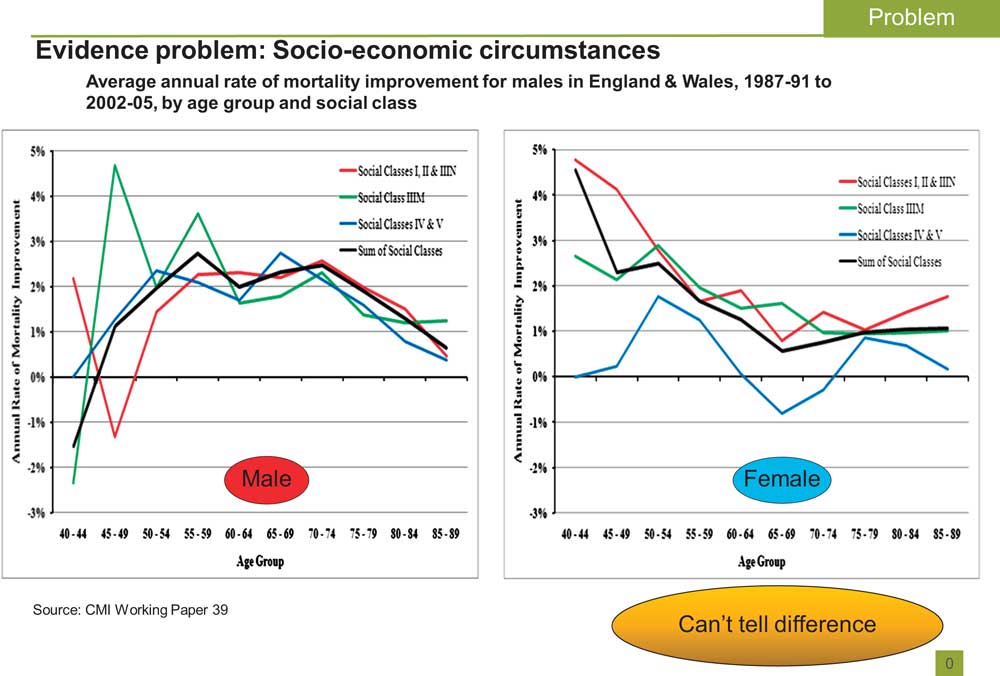
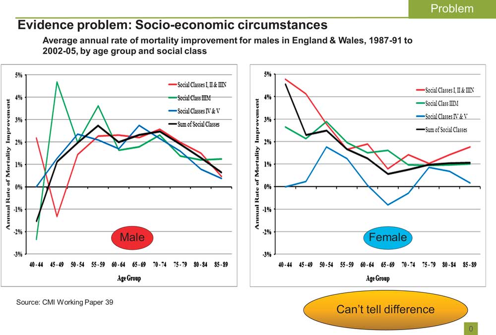
Referring to Figure 1, on the X axis we have the ages and the Y axis these are the estimated annual rate of mortality improvements between 1987 and 2005 and we see that the results are quite volatile. If we were to do an analysis we are unlikely to show any evidence of any differences between them.
Evidence problem: Socio-economic circumstances. Average annual rate of mortality improvement for males in England & Wales, 1987–91 to 2002–05, by age group and social class
The data issues and lack of market consensus have led to the insurance and pensions industries deriving mortality improvement assumptions from the total population for people in different SEC.
This would lead to the risk that the total population's experience may not be a good reflection of the experience of the sub-group. We call this basis risk.
If the assumptions derived from the total population under-estimate mortality improvement of the sub-group, this could lead to inadequate funding for the pensioners.
If the assumptions derived from the total population over-estimate mortality improvement of the sub-group, from the pricing perspective for annuitants, this could lead to missed opportunities due to over-pricing.
In addition, insurers or pension funds may want a better understanding of basis risk before using longevity derivatives based on population experience.
At the moment, I think there is a desperate need for a larger dataset, a dataset with more frequent data and more consistent data.
Our solution is to get not just 1% of England's data but 100%. This larger sample is much better than the ONS longitudinal studies that we have been using. We have yearly data between 1981 and 2007 which allows us to work out the annual rates of improvement in mortality. We have found a way to identify SEC using a well-recognised method: the index of multiple deprivation based on local deprivation of the people. It provides consistency and credibility.
All these are characteristics that have advantages over most of the CMI or ONS longitudinal data sets that have been used to study mortality trends by SEC.
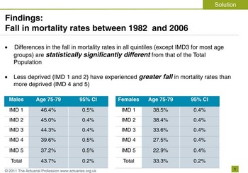
Figure 2 shows that between 1982 and 2006, the less deprived have experienced greater fall in mortality rates than the more deprived. For males aged 75–79, the least deprived quintile (Index of Multiple Deprivation (IMD) 1) have experienced a fall in mortality rates of about 46% but the most deprived quintile (IMD 5) have experienced a fall in mortality rates of about 37%. We can see a similar pattern for females. Apart from the middle quintile, the fall in mortality rates of other IMD quintiles are statistically different from that of the total population, between 1982 and 2006 for both genders and most age groups. This demonstrates the potential basis risk of using the total population experience for socio-economic sub-groups.
Findings: Fall in mortality rates between 1982 and 2006

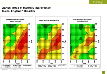
We have plotted the annual rate of mortality improvements of different IMDs (1, 3 and 5) illustrated in Figure 3.
Annual Rates of Mortality Improvement Males, England 1985–2005

These are the heat maps for the annual rate of improvement in mortality for people in different SEC. The X-axis represents time period and the Y-axis represents age. Each individual colour represents the annual rate of mortality improvement for that age in that time. The hotter the colours, the higher the mortality improvement rate.
People in IMD 1 have experienced hotter colours (more red than green) than people in IMD 5. The streak of warm colour crossing diagonally indicates the well known UK healthy cohort, a group of people who have experienced faster annual rates of mortality improvement than people born before or after that group. So, we can see here the cohort effects are more pronounced in the least deprived quintile when compared with that of the most deprived quintile.
You may ask if we should concern ourselves with the most deprived quintiles. Are they relevant to pension funds or annuity books?
Of course, it is up to each individual annuity book or pension fund to assess the distribution by SEC. But, based on our experience, we find it is not uncommon to have 20% of people living in IMD 5 areas. By weighting the pension amount, it usually represents about 15% of pension amount. I think they are relevant.
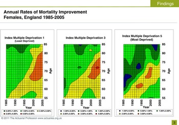
We can see a similar trend for females as shown in Figure 4. IMD 1 has hotter colours when compared with IMD 5.
Annual Rates of Mortality Improvement Females, England 1985–2005

We may ask what is the average difference in annual rate of mortality improvements between the different IMD quintiles? We know there is a difference. Is there a quick way to represent all these different IMDs by adjusting the assumption for the total population? Is the difference 0.25% p.a. or 0.5% p.a. ?
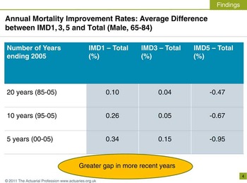
Figure 5 shows the average difference in annual rates of improvement in mortality between the different IMD quintiles and that of the total population, for males age 65–84. The average difference between IMD s and total population depends on the period of investigation – 20, 10 or 5 years ending 2005.
Annual Mortality Improvement Rates: Average Difference between IMD1, 3, 5 and Total (Male, 65–84)

Take IMD1 for example. The average difference in annual rates of improvement in mortality from that of the total population is 0.1% for 20 years ending 2005, rising to 0.26% for 10 years or 0.34% for 5 years ending 2005. For IMD 5, the average difference in annual rates of improvement in mortality from that of the total population is −0.47% for 20 years ending 2005, the gap increases to −0.67% for 10 years or −0.95% for 5 years ending 2005.
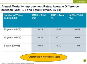
The gap is greater if we use more recent data. There is a similar pattern for females (see Figure 6).
Annual Mortality Improvement Rates: Average Difference between IMD1, 3, 5 and Total (Female, 65–84)

These differences can help us estimate the potential extent of basis risk. How differently can the various IMDs behave from the total population? What are the potential financial impacts?
To avoid being spurious, we will use ranges rounded to 0.25% p.a. to estimate the financial impact through annuity values. For example, we'll not use 0.54%, but a range of 0.5% to 0.75% p.a.
We will consider 2 scenarios:
• Scenario 1: the gap between IMDs and total population would continue perpetually.
• Scenario 2: the gap between IMDs and total population would eventually disappear.
Scenario 1: Let us look at the potential financial impact if the average gap, derived from the period 5 years ending 2005, were to continue perpetually.
For the total population, we've used the CMI 2009 Model with a long-term rate of 2% p.a. for illustration. Changing the long-term rate to 1% doesn't change the outcome of our analyses.
Take males from IMD1 for example. The average difference from mortality improvement of the total population is about 0.3% p.a., over the 5 year period ending 2005. We don't use 0.3% but the range 0.25–0.5% p.a. With this range, we calculate annuity values using different discount rates from 0 to 5%. The annuity values from these calculations are between 1% to 4.5% higher than those generated from the population's assumption.
For IMD 5, we can see up to 9% difference. These are for scenarios where the gaps continue perpetually. If the gaps disappear eventually, the financial impact would be less.
Scenario 2: The relative difference in annuity values from the population's assumption ranges from just 0.5% to 3%, rather than 1% to 9% in Scenario 1. Other scenarios are possible. Gaps do not have to stay the same or reduce. They can increase or reduce or even cross-over between the IMD groups.
We know very little about what has caused the differences in mortality improvements between people in different SEC. However, we have a lot of literature on potential reasons for differences in mortality rates between people in different SEC. A paper (“Life Expectancy; past and future variations by socio-economic group in England and Wales”, 2012) by the Longevity Science Advisory Panel, led by the late Sir Derek Wanless, concluded that there are powerful forces that keep the mortality rates of people in different SEC apart. I suggest that these forces could potentially influence future trends of mortality rates of the various SEC.
Let us look at potential factors that can influence future changes in mortality trends in SEC. These are factors which have been considered to cause differences in mortality rates between different SEC.
Wealth/Income gap
Lower income would directly disadvantage people in terms of living conditions, access to health care, nutrition and other factors leading to disadvantaged health conditions and higher mortality rates. It could also, indirectly, lead to poorer health through its association with less desirable employment conditions exposing them to work hazards, lack of control and stress.
Since the 1980s, the income gap between the rich and poor has widened, with mean income of the wealthiest 10th rising from 3 times to 4 times that of the poorest 10th of the population (Wanless et al., 2012). Any changes in the wealth or income gap between people in different SEC could influence their future trends of mortality rates.
Risk factors
People in lower SEC tend to have worse risk profiles. For example, males in the most deprived IMD quintile were 3 times more likely to be smokers and 1.5 times more likely to diabetic between the mid 1990s and 2008. A recent study has shown that people in higher socio-economic positions have experienced a greater reduction in the proportion of people who engage in multiple risky behaviours including smoking, excessive alcohol, poor diet and low physical activity levels. Changes in risk factors profile such as prevalence of smokers, alcoholics, diabetics, etc. in the different SEC could potentially influence future mortality trends.
Access to health care
Our collaboration with University College London and Liverpool University has studied the uptake of a range of surgical and medical treatments for coronary heart disease and concluded that there is no evidence of systematic differences in uptake rates between IMD quintiles. However our studies on uptake in cancer treatments have reported that patients in deprived areas were less likely to be given preferred surgical procedures for rectal, breast and lung cancers. Any differences in health care use could affect future mortality trends.
Behavioural and ‘cultural’ model
Sociologists have proposed that differences in behaviours or culture between people in different SEC could potentially explain the differences in health between SEC. For example, healthy behaviours, such as exercise, may be encouraged by peers in higher SEC. Conversely some less healthy behaviour such as smoking may be more tolerated among peers in more deprived circumstances. These would imply that changes in behaviours and culture within IMD quintiles could potentially influence future rates of improvement in mortality.
Psycho-social model
The psycho-social model proposes that people in occupations with a lower social status experience less control, autonomy, respect and reward at work. These negative experiences could induce stress and trigger hormonal actions in the body that results in depressed immunity which in turn leads to diseases.
Establishing a causal link between SEC-related stresses to historical mortality improvement patterns would be challenging. But any changes in potential difference in psycho-social stress between SEC could change the pattern of future mortality improvement between people in different SEC.
Life-course model (Bartley, 2004).
There is a view among social epidemiologists that health differences between SEC arise as a result of cumulative experience of lifetime advantageous or adverse social, biological and psychological circumstances. This approach would imply that the higher mortality risk of people in more deprived SEC is a result of embedded health disadvantages. It would be challenging to reverse health disadvantages accumulated over a life time.
Government policies
Successive governments have unsuccessfully tried to reduce inequality in health and mortality between people from different SEC. This highlights the challenge in reducing the health and mortality gap associated with SEC.
Adopting Healthcare Initiatives
A study has shown that the more educated tend to remember healthy lifestyle messages from the government. People from less deprived SEC are more likely to respond to new health initiatives, wedging the health gap between SEC groups. This might have partly explained the higher mortality improvement rates among the more affluent in the past. For example, the more affluent may have responded more quickly to anti-smoking messages. It remains to be seen if people in more deprived SEC are catching up, potentially fuelling future mortality improvement. Any effort in addressing this disparity in responding to health messages could change future mortality improvement trends between SEC.
We have obtained England's death and population data between 1981 and 2007 split by gender, IMD quintiles and 5-year age-bands. Using 3-year moving average mortality rates of 5-year age bands, we have demonstrated statistical differences between change in mortality rates between total population and all IMD quintiles, except the middle quintile, over the period 1982 to 2006. Between 1982 and 2006, males have experienced a greater fall in mortality rates than females within each IMD quintile and age-band.
Heat maps show cohort effects in all IMD quintiles. The heat maps of the least deprived IMD quintiles for both genders have warmer colours indicating higher rates of improvement in mortality. We observe that the average absolute differences in improvement in mortality rates between the most and least deprived IMD groups have widened between 1985 and 2005. This leads to uncertainty about the future projections for different SECs and basis risk.
We have examined the potential extent of basis risk using experience over the 1982–2006 period and using some potential future scenarios. These examples suggest that owners of longevity risks such as pension funds, insurers and investors would be able to assess their risk appetite and tolerance for basis risk using appropriate data and method.
Mr N. Robjohns, F.I.A (opening the discussion): The paper gives us some new insights into patterns of mortality improvement by socio-economic group and an assessment, by means of selected scenarios, of the possible financial implications of increasing mortality improvement rate differentials.
Whilst several aspects might merit further discussion, the authors have gone to some lengths to show that their main conclusions are not sensitive to the detail of the methodology.
In section 3.1, particularly Tables 1 and 2, the authors demonstrate that there have been statistically significant differences between mortality improvements by IMD quintile over the period 1982 to 2006. That is no surprise as the ONS longitudinal study tells us as much but the paper also gives us interesting new insights:
– The statistical significance holds for the differentials for each 5-year age band;
– The pattern of differences in improvement rates is remarkably similar across the age range 65 to 84; and
– The differentials have generally increased over the period 1982–2006 as the aggregate rates of mortality improvement have increased.
The paper does not reveal the absolute or relative mortality levels by IMD. If it did, I suspect the differential by IMD might be reasonably even. In contrast, the differentials in mortality improvement rates are notably skew, with relatively small differences between the improvement rates for quintiles 1 to 3 and larger differentials between quintiles 3 to 5.
Given this feature, the authors note the question of the degree of relevance of the most deprived quintile to pension schemes or annuity portfolios. I was surprised by the assertion that it is not uncommon to have about 20% of lives in a scheme belonging to IMD quintile 5. This seems at odds with data from the ONS pensions trends reports which show a significant gradient in pension scheme membership by socio-economic group and earnings.
The statistical analysis shown in section 3.1 is not extended to the analysis of differences in improvement rates over shorter time periods. It would be helpful to work the data harder so that we would know whether the larger differentials shown over the short period 2000–2005 are statistically significant too. I suspect they are, but we must recognise that even a dataset of this size has its limits. My own simple analysis suggests that the dataset might support statistically sound conclusions on the differentials currently observed on 5-year age bands and over 5-year periods, but that it may not be possible to identify statistically significant differentials over shorter periods. We are therefore able to observe differential trends over the recent past, but not to make any statement about current differentials or about detailed patterns by age.
Section 3.2 presents heat maps of annualised mortality improvement rate surfaces. These appear to show broad cohort effects for each IMD quintile. Here again it would be interesting to work the data harder to investigate the differences between them.
In its initial discussions, the Working Party which developed the CMI Mortality Projection Model considered the possibility that the peak year-of-birth for mortality improvements in the ‘golden cohort’ range might vary by socio-economic group. This could arise for example under the ‘diffusion theory of behaviour change’, where changes in health risk behaviour are adopted first among the middle classes and then diffuse through the population. That feature was not built into the CMI Model as no strong evidence could be found. However, this English population dataset may be large enough to test such a hypothesis and I urge the authors to have a go at this or to make the dataset public for others to extend the work.
Turning now to section 3.4 and the financial consequences, I note first that the authors refer to potential benefits for small to medium sized pension funds if index-based hedging were facilitated by a cheap and liquid market. The subsequent analysis considers basis risk by comparing mortality trends in different socio-economic groups with that of the population as a whole. However, small to medium sized pension funds would also need to consider the potentially greater basis risk inherent in the outcome for their specific group of lives compared with their socio-economic benchmark.
For the historical perspective (section 3.4.1), the authors evaluate the different outcomes by IMD quintile using data for 1982–2006. The differences in annuity values and survivorship appear to be relatively small, but we should note that the analysis only uses the lower triangular half of the dataset (year-of birth cohorts 1898 to 1922) and therefore misses out much of the higher mortality improvement rates and greater differentials shown elsewhere in the paper based largely on the other half of the dataset.
For the future perspective (section 3.4.2) the two scenarios used both reflect further increases in the differentials in mortality levels; scenario 1 maintains the gap in improvement rates so that the mortality rate differential continues to widen indefinitely; scenario 2 gradually equates the rates of improvement, so that the gap in mortality rates by IMD widens more slowly and eventually stabilises. The tables in the appendices allow the reader to consider some alternative scenarios, including the possibility of the mortality level differentials reducing over time, but don't allow anything more complex, such as the gap expanding for a while longer and then contracting.
Finally, many of the ideas covered attempt to explain the differences in mortality levels by socio-economic group and are difficult to extend to consideration of trend differentials. However, a recurring theme is that the least deprived groups are often ‘early adopters’ of beneficial change so that innovations which may lead to reductions in mortality are likely to show up first through faster mortality improvements for those groups than for the more deprived groups. Assuming the innovation eventually works through the population, the more deprived groups would show comparable mortality improvements later than the least deprived groups. This would lead to a pattern, for each innovation, of a widening of the differentials in mortality improvement rates and mortality levels, followed by a reversal of the difference in improvement rates and a contraction in the mortality rate gap.
The analysis for this paper covers the period 1982–2006, a period in which aggregate rates of mortality improvement have generally been increasing. It seems plausible that the least deprived socio-economic groups have been in the vanguard of experiencing the series of innovations causing these aggregate trends, and that has contributed to widening differentials in mortality improvement rates and mortality level differentials by socio-economic group.
Mortality projection bases in common use today widely assume a slowdown in aggregate improvement rates. Such a scenario implies the running-off of these past innovations, and fewer new innovations, so it seems natural to ask whether, under those conditions, we should expect a reversal of the mortality improvement rate differentials by socio-economic group and a contraction of the gap in mortality levels. At the very least we should consider, under various theories of the forces driving mortality differentials by socio-economic group, how to marry up our assumptions at aggregate and at socio-economic group level.
Mr S. D. Baxter, F.I.A: For me, the overriding theme of the paper was the very apparent difference in historic improvements seen between different groups of individuals.
We routinely use different improvement assumptions for men and women, yet the differences we see between socio-economic groups in Tables 1 and 2 of the paper are just as large; differences which, if they persist, can be financially material.
Surely it is time that, as a profession, we address this issue by allowing for socio-economic differences in our projections.
I accept that there is uncertainty in how to project these differences, but this is a challenge to which we should rise. The uncertainty of how these differences in improvements will evolve is key for all of us, regardless of whether we are in the life or pensions industry.
It is this perception of basis risk, the emotive side of the debate, which is why many clients I talk to are nervous about the population-based index market, and have welcomed the publication of socio-economic indices which mitigate this concern.
The authors highlight the uncertainty in future trends by socio-economic status by using two scenarios which lead to a spread of in excess of 10% in pensioner valuations, depending on the socio-economic mix of the portfolio. The potential impact they show is in stark contrast to that reported in more theoretical analyses of basis risk, which often make the unjustified assumption that underlying trends will be highly correlated.
It is worth noting that the two scenarios chosen by the authors are far from extreme, specifically a continuation of the existing gap in improvements, or a narrowing of the gap in improvements. In practice, there are plausible scenarios which would lead to much wider valuation spreads (perhaps in excess of 20%), for example if the gap in mortality improvements continued to widen.
The paper highlights how different socio-economic groups have experienced different historic mortality improvements. Further, the paper provides an excellent summary of plausible reasons for these differences, and thus why differences may persist into the future. Having stochastic models which allow for the prospect of different, imperfectly correlated trends between socio-economic groups will release a hitherto unrecognised diversification benefit for many insurers and reinsurers.
Finally, perhaps I can remove a little of the uncertainty and provide some potentially good news from a reserving perspective. The data collected by Club Vita enables us to add a few more years onto the end of the heat maps produced by the authors. This latest data provides early indications that for many ages mortality improvements may currently be lower for the capital intensive higher socio-economic groups compared to the ONS population data embedded in recent versions of the CMI model.
Mr A. G. Sharp, F.F.A: I was struck by a comparison of lower super output areas (LSOAs) (some 32,000 LSOAs covering about 1500 persons each) with postcodes (some 1.6 m residential postcodes, covering about 30 persons each on average). Clearly we are still some way short of the longevity modellers ideal of postcode specific mortality rates and improvements.
One limitation of the results of the research is the lack of results for ages above 85. I can understand this, given the paucity of the data available for advanced ages. Given that, and the current uncertainties about old-age improvements from the latest ONS census data, I suspect that many practitioners will look at the results in Tables 11 and 12 and may then make a small subjective change to their improvements assumptions in the light of what is known about the socio-economic make-up of their portfolio, rather than implement a more detailed modelling approach. There is of course more concern about underestimating improvements than overestimating them.
Finally, as always, we are left with the dilemma as to how much our modelling of the past should guide any forecasts of the future. For that we need a much wider discussion about social policy and provision of healthcare.
Prof. M. Bartley (guest, Professor of Medical Sociology at University College London): Modifiable areal unit problem is a geographical term. It means that when you have an officially defined area of any kind – travel to work area, super output area or post code – it is drawn in a way which is going to leave out a lot of the people who share the characteristics of the people inside the area, such as low income. They will also include a lot of people with characteristics like high income which mean they should be outside that area. This is true however you chart out the area.
Modern Geographical Information System software allows one to design an area however you want, by putting together postcodes. You can gather together your postcodes until you have areas of the same number, average population number but which have been defined by other kinds of data which are available. In this way you could have a much purer representation of the characteristics in which you are interested.
One thing which might be a problem from the insurance point of view is if you allocate somebody a risk on the basis that they are a resident in a certain area, they might move into a different area. If the risk has anything to do with characteristics in the area, that person's risk level is going to change. This is not just some of the characteristics that confer risk might be to do with exposures in the area, for example, poor housing or near to an asbestos plant, so that when you move away you change your risk. The effect may also be on the cultural side, to go back to one of Mr Lu's categories, since there is now increasingly good evidence that the behaviour of people who surround you influence your own health risk behaviours such as unhealthy diet, smoking or taking exercise. It might be worth taking into account that cultural and geographical changes experienced by people moving from one area to another might change their risk profile.
Mr A. P. Bell (student): In Appendix D there is discussion around a potential problem with the SEC method used i.e. determining the relative deprivation level for each area based on index values in 2007, and assuming that these have stayed constant over the 25-year period of analysis.
You acknowledge that in practice some areas may have become relatively more deprived over the period, and others may have become relatively less deprived. This would seem to exaggerate the effects you are observing, for example, those areas which become less deprived would be expected to inherit relatively lower mortality rates over time even if the rate of improvement does not vary significantly by SEC.
Given that you have made estimates of the level of transition between different deprivation quintiles,
• Have you attempted to adjust for the effect of these transitions?
• If so, does this alter your conclusion (or the strength of your conclusion) that past improvements have typically been higher for those at lower deprivation levels?
Prof. D. Blane (guest; Professor of Medical Sociology at Imperial College London): Before the Second World War a lot of the older members of the pre-WWII Boyd Orr cohort had dietary habits which were poor. What was considered a good diet was a diet that had a lot of red meat, a lot of butter, full cream milk, a lot of cheese, and the only people who ate what is now called a healthy diet were poor Scottish people who ate porridge oatmeal and oily fish like herring, and agricultural workers who took part of their wages in vegetables and milk from the farm.
The second thought is because of what Professor Bartley was talking about in terms of the varied socio-economic composition of a particular area: the data which we have been shown is very conservative. They are likely to be under-estimates because in the more affluent areas there will be a fair number, maybe up to 30%, of people who are less affluent than average. In deprived areas there will be maybe up to 30% of people who are more affluent than the average in their area. There will be a concertina-like effect. It seems to me that the effects shown in terms of the actuarial implications are very serious. If you use the population average and your insurance base is drawn from more affluent people, then you are going to go bankrupt because everyone is going to live much longer than you are expecting. Similarly, if you have a pension scheme or a state pension scheme, which has a higher proportion of people from the more disadvantaged group, then you are going to charge too much because people are going to die more quickly than you would expect from the population average.
The Chairman: In August, Olshansky et al. in the US published an analysis of differences in life expectancy due to race and educational qualifications: “Differences in life expectancy due to race and educational differences are widening, and many may not catch up”.
Of particular interest was the fall in the expectation of life for white people with no high school diploma. At the bottom end of the education spectrum, between 1990 and 2008 white men's expectation of life has fallen by three years; white women's expectation of life has fallen by five years.
I wondered whether it might at some stage be possible to cut the figures by education rather than by SEC?
Dr M. Bajekal (replying): Mortality differentials by education is a useful alternative marker of socio economic status. However educational attainment is not recorded on the death certificate. You would have to follow up people in the census to calculate mortality rates by education categories.
Mr Sharp asked why we are using LSOAs rather than the more numerous postcodes. The reason we do not use postcodes as a segmenting factor, is because all the products that are available using postcodes, like Mosaic and so on, are classificatory systems. They do not have a continuous numerical score attached to rank different types of areas. The LSOA is the lowest level of geographical aggregation at which you have a deprivation score. LSOAs can thus be ranked by their score and grouped into equal fifths by increasing deprivation. So we did the analysis that way. The way the LSOAs are designed are for statistical purposes and their boundaries will remain fixed over time. Boundaries are also drawn as far as possible to contain housing of a similar type to capture a neighbourhood with a similar social profile. There are about a 1000 adults per LSOA and this varies little across all LSOAs.
Taking up the other points about internal migration and gentrification of areas and how these affect our findings. This is a crucial point. If we had deprivation indices on a fixed small geography right the way back from 1981, 1991, 2001, and so on for each census year, we would have used these. We were forced to use something which was only available for the end of our time series (i.e. 2007) and not for all previous years because of the way the 7 domains in the (IMD) have been defined. We don't have equivalent variables in previous years and certainly not at the LSOA level of geography.
But we also need to remember that when you split the whole of England into quintiles you are talking about  $$$6\tfrac{1}{2}$$$
thousand of these small areas in each quintile group and about 7 million people in each group. So there will be a lot of movement in terms of individual ranking of each LSOA over time: that is, a lot of movement within a quintile group. There will be less movement of areas between quintile groups. In Appendix D, we looked at the stability of LSOA quintile ranking over time. About three-quarters of areas in the top and bottom quintile stayed within their quintile group across 20 years.
So there is a fair amount of stability in relative positioning of areas over time. For example, if we look at Booths map of London, you find the same areas are deprived now as they were 100 years ago. IMD is the best proxy measure of SEC that we have, so we have used that.
Areas might stay in their relative positions over time with respect to deprivation, but even if the ranking remained markedly stable, there may be internal migration of healthy people up the scale (or gentrification) and equally, a downward migration of unhealthy people to poorer areas. So I have looked at that using published literature which analysed internal migration in the longitudinal study. The study contains linked census and vital event data for 1% of the population of England and Wales. The study examined internal migration patterns of people from 1971, 1981 to 1991, quantifying movement between deprived and affluent areas and the net effect of these on widening inequalities in mortality.
The authors concluded that selective migration has an effect on area inequalities. Healthy people do move up, unhealthy people do move down. This results in a widening of inequality over time as measured at an area level. But the scale of selective migration is not of the level where it makes a material difference, or what you would call a significant impact on the measurement of inequalities in health.
The next question was about the issue of health being included as one of the domains in the IMD. The health domain includes mortality rates as well as long term illness rates for an LSOA. So we repeated some of our analyses removing just the health domain from the composite IMD score. We found it made very little difference to our results. This is because the loading on the health domain is so much lower than that for the wealth and employment domains and furthermore all the domains are also highly correlated with each other.
A very interesting question which Mr Robjohns raised was about reversals in mortality improvement rate differentials by socioeconomic group i.e. rates falling faster in the more deprived groups. We don't know what will happen in the future but what we do know is that in the last decade, despite the fact that falls in smoking have slowed down, and other risk factors, like BMI and diabetes are rising in all the social classes, not just the most deprived, mortality rates have been falling even more steeply from 2000 onwards than in the previous period. There is no reversal; in fact, we see the differential is widening. We modelled this to look particularly at factors contributing to the widening differentials in heart disease mortality because that is the main driver of the fall in total mortality over the last 25 years. The model included the contribution of change over time in seven risk factors and the increased uptake of 49 specific CHD treatments, within each quintile group. Despite taking account of all these factors we were not able to explain all of the more rapid fall in mortality in the most affluent deprivation group. We do not understand why the mortality improvement rates in affluent areas continue to be higher than in deprived areas. So currently, there is no sign of reversal in mortality improvement rates.
For our future research, the upshot of our CHD findings is to try and understand what is it about affluent areas that is causing their mortality improvements to be so much more rapid than in other areas? I was surprised by Mr Baxter's more recent analysis that the mortality improvement rates for more affluent people in the Club Vita population fell to below the national level (ONS). We will need to update out quintile-based mortality trend series to 2010 to see if we get similar results.
Mr Lu (replying): I refer to Mr Robjohns’ questions about mortality rates of people between different SEC and differences between them. We have not presented the results here because this is just one of the papers that we intend to publish. We have been working on the changes in life expectancies and mortality rates will certainly be an area that we will look into and present in some papers. We will look into the hypothesis of diffusion theory: the hypothesis that higher social groups are quicker to adopt new health knowledge therefore experience faster mortality improvements first.
If this were true, you would expect people in high socio-economic groups to experience a rise in mortality improvement over time and that would be followed by lower socio-economic groups. We see that both IMD 1 and 5 have experienced a sharp rise in improvement in mortality around 1995. So we probably need some more detailed datasets to answer that question.
We have seen people in higher socio-economic group tend to remember government health messages and take advantage of screening earlier. So it remains to be seen if people in higher socio-economic group have given up smoking first followed by the lower socio-economic groups, resulting in faster mortality improvement among the higher socio-economic groups only to be followed by those in lower socio-economic groups
But we need to bear in mind that smoking is not the only factor that causes differences. There are many other factors. One example is the life course model, which says differences in mortality are as a result of a life long accumulation of advantages or disadvantages in terms of health. It is very difficult to reverse lifelong accumulation factors in a short period of time.
Mr Robjohns and Mr Baxter asked about the possibility that differences in mortality improvements could widen. Yes, it is possible: there is no reason why it has to converge or stay the same. The impact can easily be modelled.
Mr P. H. Simpson, F.I.A: In response to one of the earlier questions about the decline in life expectancy of some of the lower socio-economic groups in the US, part of that has been thought to be associated with the effect of the lack of social security but, more particularly, the lack of a medical safety net in the US. You tend to have a much greater potential for downside, particularly when you are looking at second or third generation families primarily living off state benefits. It tends to be the lifelong access to medical insurance, Medicaid or the lack of that in the US, that it is one of the reasons why we have seen some quite startling declines in longevity, not just for whites, but more widely across the lower socio-economic classifications in the US.
One thought is around the lack of higher age data. Although there is uncertainty involved, is there any ability to put boundaries around that uncertainty in what may be the difference in the higher ages? It seems to me that there has been some uncertainty and some difference in practices in the UK about whether the decline in mortality at the higher ages is level, accelerating or is going to trend back down to some lower average.
Certainly I believe that, internationally, some of the highest increases in mortality have been reported at very high ages. I think in Japan there was a cohort born about 1914 to 1920 which was reported to have shown a 6% or 8% per annum increase: even in 80s and 90s this is a very high level. Have there been any thoughts around putting bounds around the uncertainty relating to older age data? We cannot say what the uncertainty is but we might say what the worst-case scenario or the best case scenario is, based on evidence from other countries, to overcome the lack of data at older ages.
What does all this mean, particularly for life insurers with a significant longevity exposure, for Solvency II? I think you have demonstrated that there are statistically significant differences between the cohorts, and classifications. Even for a standard model firm, when it is looking at its Own Risk and Solvency Assessment (ORSA) it might wish to think whether these are risks that are not captured in the standard model. The latest guidance on ORSA states that if you have material risks not covered by standard model you should quantify them.
I wonder whether this is going to push more firms down the partial internal model ultimately for Solvency II. Obviously we have seen, coming back to the age issue, that at age 85 the combination of your SCR and risk margin could be quite high compared to someone aged 65. If you have an elderly portfolio, there might be significant financial benefits in trying to understand whether you have a good, or not so good, elderly portfolio based on the criteria we have been discussing.
Mr R. C. Willets, FFA (closing the discussion): This paper is much more than just a review paper of work that other people have done: it is a substantive piece of original research which adds to the pool of knowledge in this sphere. It demonstrates the value of collaboration between actuaries and professionals in related disciplines.
Mr Sharp mentioned that data is very much a key in this area. I am sure not everybody will have managed to get through to Appendix D, but it is definitely worth a read.
I thought of the potential impact of selective migration, people moving from one group to another over time, and whether that had a distorting impact on the results. When I read the paper, it was certainly my suspicion that the migration might have a material, albeit small, impact on results, particularly for groups one and five.
I thought the points made about heterogeneity within geographical regions were also good ones. Professor Blane mentioned heterogeneity leads to an under-estimate of the differentials of improvement by social class. Professor Bartley mentioned a way of getting round that, which Dr Bajekal then countered.
I am also quite interested in hearing more about some of the messy issues to do with data, issues to do with classification of deaths and populations into different groups. Perhaps that is one for later, however I was interested in how difficult it was, say, to allocate somebody who had died in, say, 1981, to a geographical area to find in 2007, and whether it would become easier over time to allocate people to different groups among the deaths and among the populations and whether that introduced any bias, for example.
Moving on to the issues of what has caused the differentials and what is likely to happen in the future, I was not at all surprised there was a lot of debate focused on whether differentials might persist in the future and what the future was likely to bring. Professor Blane mentioned it is very difficult to project the future, which is obviously something, as actuaries, of which we are very much aware.
I had a lot of sympathy with Mr Robjohns’ point that the last 20 or 25 years have been quite an unusual period of time. Improvements have been more rapid than they ever have been in the higher ages and we have seen, generally speaking, accelerating improvements over that period of time. The diffusion theory would lead you to think, if you assumed improvements were going to decelerate in the future, that differentials in mortality by social class might reduce. It may be of particular note that the five-year period where the differentials appear to be greatest was from 2000 to 2005. That period of time saw particularly rapid improvements and accelerating improvements. Since 2005, I think on an aggregate level improvements appear to have plateaued off a little bit. I thought it was very interesting the point Mr Baxter was making about the Club Vita data showing more recently the higher social class groups were showing lower improvements than the aggregate. Those two things might be related.
I think it is extremely difficult to predict what is going happen in the future. I have a lot of sympathy with Mr Baxter's view that we should have differential assumptions for different social classes. But what should those assumptions be? Should they be more rapid for the higher social class groups than the lower social class groups? I see the future situation as being quite complex. I can certainly see improvements due to causes such as cancer – improved treatments for cancer, better understanding of the drivers of cancer – and can well imagine that we will see widening social class differentials in improvements from that particular cause.
When it comes to something like heart disease, there is such a pronounced social gradient in mortality now, there may well be a narrowing of the social class differential in that particular cause. You have quite complex patterns going on underneath the surface.
It occurred to me that it would be interesting to see whether the analysis that the authors have done could be extended to examine how past trends by different cause of death groups have varied over time, for the different quintiles, to better-understand what may have caused past trends and really focus in on what might be happening in the most recent data.
The paper is a very important, but so far little-understood, area in actuarial work into longevity. I am hoping that this paper will serve to kick-start research in this field.
Dr M. Bajekal (replying): I thought I would respond first to the question about data for older ages. This is exactly where we are heading in the next phase of our research. We are requesting more granular data for 85+ from the ONS.
The problem here is that you do not have accurate denominator counts of population exposed to calculate reliable rates. We do have deaths on an individual basis. All that you can do is calculate mortality rates centred around the census year. So what you are trying to do is to look at mortality data pooled over five year around the census year and using accurate population denominator counts from the census to calculate robust age- sex- specific rates for the oldest old. But then you have to do it for 1981, 1991, 2001, and so on in order to examine underlying trends in rates for the oldest old. That makes it a slightly larger project.
Coming to Mr Willets’ points, in terms of looking at analysing past trends by cause of death, again that is something we have started to do. I presented to the Institute's actuarial conference last year on decomposition of life expectancy change by cause of death both across time and between deprived social groups.
Mr Willets also asked about the ‘messy’ data issues of allocating 1981 post coded deaths to 2007 LSOA boundaries. The way the ONS does this is that from at least 1981 onwards, deaths (postcodes) were allocated to electoral wards. Historically, we have had something called ‘statistical wards’ whose geography remained fixed from 1981 onwards. Statistical wards have then been allocated to LSOAs. So all deaths from 1981 onwards were mapped onto fixed wards and an algorithm was used to distribute these proportionately to LSOAs. So the method for allocation is fairly consistent over time. There will be some mismatch, but again it won't materially affect our findings at the high level of aggregation (quintiles) we've used.
Mr Lu: I think the solution is to get the data. There is an increasing need for mortality data above age 85 because there are more people above age 85 now. It used to be acceptable to have detailed data up to age 85, but it is now less acceptable for most analyses. We need data up to ages 100 or 105. That is something that we need to work together. In terms of risk management and modelling for different socio-economic groups, I think it depends on how concentrated are individual pension funds towards certain socio-economic groups.
For many final salary schemes, the issues are less problematic because the socio-economic distribution may not deviate too far from that of the general population, even after allowing for the fact that the more affluent are associated with more of the pension's liabilities through their higher pension amounts.
There were a lot of comments on and suggestions on length of data. We take on board Mr Willets point about what happens after 2005 and the work on the older ages and causes of death. It is something that we have been keen to work on as well. It is important to understand what is happening in terms of causes of death and project them forward into the future. There may be a limit to how much mortality rate could fall for some causes of death.
The Chairman: It has been a pleasure to have been part of the discussion. I would very much like to thank Mr Lu, Dr Wong and Dr Bajekal. Dr Wong and Dr Bajekal are particularly to be thanked as they are not actuaries, although Dr Bajekal is on our Mortality Research Steering Committee and is very valuable in keeping those links with other professions.