1 Introduction
Despite its long research history, the physics underpinning the breaking of water waves has remained incompletely understood, including prediction of its onset and strength. Yet this knowledge is of fundamental importance in quantifying atmosphere–ocean exchanges, determining structural loadings on ships and platforms, and optimising operational strategies for maritime enterprises.
Many criteria for predicting breaking onset of water waves have been proposed since the pioneering study of Stokes (Reference Stokes1847). These criteria arise from theoretical arguments based on idealised models, numerical simulations, laboratory experiments and field observations. However, while adding many insights, these approaches have not yielded a robust breaking threshold for phase-resolved waves in the physical domain, reflecting the complexity of the underlying dynamical processes. In fact, there is a glaring absence of a precise definition of breaking onset.
Briefly, it has long been considered that breaking is a process with a threshold, with criteria for predicting breaking onset falling into three categories: geometric, kinematic and energetic. The majority of breaking criteria have been based on a geometric or kinematic threshold, and mainly limited to plane (2D) waves. Geometric threshold variables have included wave steepness, wave asymmetry, maximum theoretical (global) steepness and the occurrence of a transient vertical segment on the forward face of the wave crest; kinematic threshold variables have included the Lagrangian crest acceleration and the ratio between crest fluid speed and phase speed. The recent comprehensive review by Perlin, Choi & Tian (Reference Perlin, Choi and Tian2013) provides an excellent overview of the collective observational and theoretical effort and outcomes based on kinematic/geometric approaches. The recent contributions of Shemer (Reference Shemer2013), Kurnia & van Groesen (Reference Kurnia and van Groesen2014), Shemer & Liberzon (Reference Shemer and Liberzon2014) and Shemer & Ee (Reference Shemer and Ee2015) add to this otherwise exhaustive coverage. Overall, current knowledge does not support a kinematic or geometric criterion that provides a generic threshold that differentiates breaking from recurrent behaviour for deep water waves. While the vertical tangent segment and kinematic criteria provide valid a posteriori conditions for breaking onset, they provide no dynamical insight or advance warning of imminent breaking (Pomeau et al. Reference Pomeau, Berre, Guyenne and Grilli2008; Bridges Reference Bridges2009).
A third approach based on dynamical criteria has been explored to explain the onset of breaking. This concept is based on the evolution of the intragroup energy flux, which causes the tallest crest of an unsteady wave group to break when a local stability threshold is exceeded. Monitoring of the energy flux field in this highly nonlinear unsteady flow environment makes rigorous analysis difficult. The overview article by Tulin & Landrini (Reference Tulin and Landrini2000) highlights the very insightful inroads made by Tulin and his collaborators over the previous decade into unsteady nonlinear wave group evolution and breaking, based on intragroup energy flux theory, simulations, observations and analyses. One of the key results they proposed from their studies is that breaking onset is initiated within a wave group when a crest particle speed exceeds the linear group speed. Pending verification of its general validity, this criterion is able to signal breaking onset much earlier than the traditional kinematic criterion.
Subsequently, Banner & Tian (Reference Banner and Tian1998), Song & Banner (Reference Song and Banner2002) and the experimental study of Banner & Peirson (Reference Banner and Peirson2007) investigated a growth rate based on a parametric energy convergence rate for 2D wave groups, using a frame of reference that tracks the wave group maximum. Perlin et al. (Reference Perlin, Choi and Tian2013) discussed the merits of this approach based on the further study of Tian, Perlin & Choi (Reference Tian, Perlin and Choi2008) for 2D wave breaking. Very recently, Derakhti & Kirby (Reference Derakhti and Kirby2016) reported very encouraging support for this approach in their numerical study of unsteady 2D wave packets in a model framework that can accommodate sequential (multiple) breaking events as the packet evolves. They confirmed the presence of systematic crest/trough leaning motions, as investigated in detail in Banner et al. (Reference Banner, Barthelemy, Fedele, Allis, Benetazzo, Dias and Peirson2014). In the present study, we revisit this local energy growth rate approach for both 2D and 3D breaking onset simulations, for which our findings are given below in § 4.3.
Finally, significant additional challenges arise in representing wave breaking in broad-banded directional sea states in the spectral (wavenumber–frequency) context. This is the domain presently used for computing ocean wave forecasts (e.g. see Chalikov & Babanin Reference Chalikov and Babanin2012). In that context, there is even less consensus on how to predict/identify breaking events. However, this is beyond the scope of the present paper, where we focus on wave breaking in the physical space–time domain.
2 Rationale underpinning our breaking onset threshold investigation
Present understanding of the physics underpinning wave breaking onset in the physical domain is fragmentary, including a precise definition. This has precluded reliable prediction of wave breaking onset even in controlled laboratory and numerical wave basin conditions. Our investigation directly addresses this time-honoured knowledge gap.
Based on energy flux considerations, we propose a new breaking onset threshold parameter. The behaviour of this parameter in the wave crest region is found to be of central importance. A new definition for a generic breaking onset threshold emerges naturally. Through an ensemble of numerical simulations of diverse nonlinear wave packets in both deep and intermediate depth water over a flat bottom, we establish the existence of a breaking onset threshold band for this parameter, determining its upper and lower bounds. Below the lower bound of the proposed breaking threshold band, steepening carrier waves evolve through the packet envelope maximum without the occurrence of a vertical tangent in the wave surface profile. All maximally steep non-breaking carrier waves exist below this lower bound, which we also refer to as the maximum recurrence threshold.
Thereafter, the smallest increment in the crest wave energy density (e.g. as produced by increasing the wave paddle amplitude) enhances the modulational energy flux within the unsteadily evolving chirped wave packet. Subsequent enhancement of this energy flux at the envelope maximum occurs through dispersive focusing mediated by the chirped packet (see Longuet-Higgins Reference Longuet-Higgins1974; Rapp & Melville Reference Rapp and Melville1990). This causes the breaking onset parameter at the tallest carrier wave crest to increase irreversibly above this lower bound. During further evolution, if our proposed breaking onset threshold is exceeded, breaking initiates with a significant change in the carrier wave crest appearance, and irreversible degeneration proceeds, as illustrated in figure 1 of Duncan (Reference Duncan2001). As discussed in detail in §§ 3.1 and 3.2 of Duncan (Reference Duncan2001), the ensuing shape of an actively breaking crest depends on the wave scale, the influence of surface tension and the strength of the breaking, which reflects the energy convergence rate at the wave crest. The strength of the breaking event is an unknown function of the magnitude of the breaking parameter above the threshold, with the smallest exceedance margins associated with very weak (i.e. marginal) breaking.
For long carrier wavelengths, the evolution to breaking leads to plunging jets of varying size relative to the wavelength: the lower the energy input rate to the wave, the smaller the plunging jet. For short wavelengths, the jet formation is modified by surface tension and has been investigated in detail with boundary element calculations, theory and experiments (e.g. Tulin & Landrini Reference Tulin and Landrini2000). When the wavelength exceeds approximately 2 m, breaking starts with the formation of a small plunging jet, just as it does when the surface tension vanishes. As the wavelength is decreased, surface tension forces become relatively larger and the jet tip becomes rounded. For wavelengths less than approximately 0.5 m, the jet is replaced by a bulge, and capillary waves appear upstream of the leading edge (toe) of the bulge, as shown in figure 1 of Duncan (Reference Duncan2001). In the present investigation, surface tension is not included explicitly. However, we show below (in § 5.5) that its estimated effect on our proposed generic breaking onset threshold is negligible for wavelengths longer than 1 m.
In this study, we use a fully nonlinear wave code capable of capturing the initial stage of crest overturning, including the critical visible signature of a transient vertical tangent on the forward face of the wave crest. The results from this code are used to determine the upper and lower bounds of our proposed breaking onset threshold band. It should be noted that we do not directly solve the instability problem for breaking onset, nor does our model provide information beyond the initial stage of crest overturning for waves that exceed our breaking threshold. In common with many other studies, this choice of using strongly chirped wave packets which focus rapidly minimises the evolution time and fetch to breaking, or recurrence, and hence the CPU time. It also reduces the adverse Lagrangian drift implications for the computational grid (see the end of § 3.2 for details). However, the high chirp rate also restricts our attention to weak breaking cases, as further small increments in paddle amplitude only produce wave breaking at the paddle.
Our breaking onset parameter is formulated as the local energy flux relative to the local energy density, normalised by the local crest speed, and is operative throughout the subsurface region including the wave surface. For the condition of zero surface pressure, its projection on to the wave surface reduces to a simple quasi-kinematic form involving the ratio of the surface fluid speed
 $u$
to the crest point speed
 $c$
. We note that the boundary geometry does not enter the breaking onset criterion explicitly, so it is potentially applicable to variable depth bottom topography scenarios.
In this study, we analyse 2D and 3D chirped packet cases with an appreciable range of bandwidths and water depths. For the 2D cases, the parameters vary from five to nine waves in the temporal packet, and the depth varies from
 $\unicode[STIX]{x1D706}_{p}$
to
 $0.2\unicode[STIX]{x1D706}_{p}$
, where
 $\unicode[STIX]{x1D706}_{p}$
is the reference wavelength at the wavemaker. We also include a targeted set of 3D cases with the most severe lateral convergence. This comprises a 3D deep water packet case with five waves, and a shallower water 3D case with a depth restricted to
 $0.25\unicode[STIX]{x1D706}_{p}$
and nine waves in the temporal packet. Both 3D cases support our proposed breaking onset criterion, so the in-between cases with respect to lateral convergence rate, relative water depth and packet bandwidth should also conform.
For this class of wave packets, the results establish the existence of a generic narrow threshold band for breaking onset, for which
 $u/c$
is found to be appreciably lower than the traditional kinematic breaking criterion of
 $u/c>1$
. As foreshadowed above, the resemblance of the surface projection of our breaking onset threshold to a kinematic criterion is fortuitous. It only takes this form for zero surface pressure forcing conditions. Its intrinsic dynamical nature is confirmed by two additional factors: the concomitant subsurface threshold does not reduce to a kinematic form and the breaking threshold
 $u/c$
ratio is considerably below unity.
As reported below, the results from our numerical investigation for deep and intermediate depth water waves are found to agree closely with measurements from our companion observational studies by Saket (Reference Saket2017), Saket et al. (Reference Saket, Peirson, Banner, Barthelemy and Allis2017, Reference Saket, Peirson, Banner and Allis2018). These observations also support the validity of our proposed breaking onset threshold for moderate wind forcing and also for modulationally focusing bimodal wave packets.
3 Methodology
3.1 Wave generation
Wave groups, either 2D or 3D and in deep or intermediate depth water over flat bottom topography, were generated using a bottom-hinged flap-type snake wavemaker at one end of the tank. The motion
 $X_{p}(t,y)$
of the wavemaker flap at the lateral location
 $y$
followed the Class 3 ‘chirp packet’ motion from Song & Banner (Reference Song and Banner2002) (this is implicit hereafter in the C3 designator in each documented run file):
 $$\begin{eqnarray}\displaystyle X_{p}(t,y) & = & \displaystyle -0.25A_{p}\left(1+\tanh \left(\frac{4\unicode[STIX]{x1D714}_{p}t}{N\unicode[STIX]{x03C0}}\right)\right)\left(1-\tanh \left(\frac{4(\unicode[STIX]{x1D714}_{p}t-2N\unicode[STIX]{x03C0})}{N\unicode[STIX]{x03C0}}\right)\right)\nonumber\\ \displaystyle & & \displaystyle \sin \left(\unicode[STIX]{x1D714}_{p}\left(t-\frac{\unicode[STIX]{x1D714}_{p}C_{ch}t^{2}}{2}\right)+\unicode[STIX]{x1D6F7}(y,X_{conv},Y_{conv})\right),\end{eqnarray}$$
where
 $t$
is the time,
 $A_{p}$
is the amplitude of the paddle motion,
 $N$
is the number of waves in the temporal wave packet,
 $\unicode[STIX]{x1D714}_{p}$
is the baseline driving frequency of the paddle, with corresponding linear wavenumber
 $k_{p}$
, and
 $C_{ch}=1.0112\times 10^{-2}$
specifies the chirp rate used in this study. The phase
 $\unicode[STIX]{x1D6F7}(y,X_{conv},Y_{conv})$
specifies the coordinates of the point of linear convergence (see Dalrymple & Kirby Reference Dalrymple and Kirby1988; Dalrymple Reference Dalrymple1989):
 $$\begin{eqnarray}\displaystyle & \displaystyle \unicode[STIX]{x1D6F7}(y,X_{conv},Y_{conv})=k_{p}y\sin \unicode[STIX]{x1D703}(y)+k_{p}(X_{conv}\cos \unicode[STIX]{x1D703}(y)+Y_{conv}\sin \unicode[STIX]{x1D703}(y)), & \displaystyle\end{eqnarray}$$
 $$\begin{eqnarray}\displaystyle & \displaystyle \unicode[STIX]{x1D703}(y,X_{conv},Y_{conv})=\arctan \left(\frac{y-Y_{conv}}{X_{conv}}\right), & \displaystyle\end{eqnarray}$$
where
 $\unicode[STIX]{x1D703}$
is the focal angle at location
 $y$
along the paddle. The downstream boundary opposite the wave paddle is a fully absorbing boundary condition, as in Grilli & Horrillo (Reference Grilli and Horrillo1997).
3.2 Numerical wave tank
There has been growing interest in the development of three-dimensional models which inherently incorporate nonlinearity and associated dispersion effects. The broad-bandedness in both frequency and direction of real sea states poses significant challenges in numerical simulation. High-order spectral expansion approaches using efficient fast Fourier transform solvers for application to 3D waves have been developed (e.g. Ducrozet et al. Reference Ducrozet, Bonnefoy, Le Touze and Ferrant2012; Fedele et al. Reference Fedele, Brennan, Ponce de León, Dudley and Dias2016), but do not permit the simulation of overturning waves. Another option is to solve the full Navier–Stokes equations (Park et al. Reference Park, Kim, Miyata and Chun2003), but viscous flow solvers tend to be too dissipative and computationally time-consuming.
Numerical models of 3D potential flow wave propagation can be divided into three main categories: (i) boundary element integral methods (BEMs), e.g. Baker, Meiron & Orszag (Reference Baker, Meiron and Orszag1982), Bateman, Swan & Taylor (Reference Bateman, Swan and Taylor2001), Clamond & Grue (Reference Clamond and Grue2001), Grilli, Guyenne & Dias (Reference Grilli, Guyenne and Dias2001), Xue et al. (Reference Xue, Xü, Liu and Yue2001), Hou & Zhang (Reference Hou and Zhang2002), Fructus et al. (Reference Fructus, Clamond, Grue and Kristiansen2005), Guyenne & Grilli (Reference Guyenne and Grilli2006), Fochesato, Grilli & Dias (Reference Fochesato, Grilli and Dias2007); (ii) finite element methods (FEMs), e.g. Ma, Wu & Eatock Taylor (Reference Ma, Wu and Eatock Taylor2001); (iii) spectral methods, e.g. Dommermuth & Yue (Reference Dommermuth and Yue1987), West et al. (Reference West, Brueckner, Janda, Milder and Milton1987), Craig & Sulem (Reference Craig and Sulem1993), Nicholls (Reference Nicholls1998), Bateman et al. (Reference Bateman, Swan and Taylor2001). Spectral methods based on perturbation expansions are known to be very efficient.
These methods reduce the water wave problem from one posed inside the entire fluid domain to one posed on the boundary alone, thus reducing the dimension of the formulation. These approaches have been summarised recently by Ma (Reference Ma2010). BEM techniques are efficient for representing wave propagation and overturning until the wave surface reconnects (Grilli & Subramanya Reference Grilli and Subramanya1996).
The present study used a boundary element numerical wave tank (hereafter NWT) code called WSIM, which is a 3D extension of the 2D code developed by Grilli, Skourup & Svendsen (Reference Grilli, Skourup and Svendsen1989) to solve the single-phase wave motions of a perfect fluid. It has been applied extensively to the solution of finite amplitude wave propagation and wave breaking problems (see chap. 3 of Ma Reference Ma2010).
The perfect fluid assumption makes WSIM unable to simulate breaking impact subsequent to surface reconnection. However, its potential theory formulation enables it to simulate wave propagation in a CPU-efficient way, without the diffusion issues of viscous numerical codes. The simulation of wave generation and development of the onset of breaking events can be carried out with great precision, as shown by Fochesato & Dias (Reference Fochesato and Dias2006) and Fochesato et al. (Reference Fochesato, Grilli and Dias2007).
WSIM has been validated extensively for wave evolution in deep and intermediate depth water and shows excellent energy conservation (Grilli et al. Reference Grilli, Skourup and Svendsen1989; Grilli & Svendsen Reference Grilli and Svendsen1990; Grilli & Subramanya Reference Grilli and Subramanya1994, Reference Grilli and Subramanya1996; Grilli & Horrillo Reference Grilli and Horrillo1997; Grilli et al. Reference Grilli, Guyenne and Dias2001; Fochesato Reference Fochesato2004; Fochesato & Dias Reference Fochesato and Dias2006; Fochesato et al. Reference Fochesato, Grilli and Dias2007). Its kinematical accuracy has been validated against the analytical solutions for infinitesimal sine waves in Phillips (Reference Phillips1977).
WSIM uses a BEM to compute field variables. The 16-node quadrilateral elements provide global third-order precision, and high-order tangential derivatives needed for the time discretisation are computed in a local 25-node quadrilateral element curvilinear coordinate system giving fourth-order precision. A fast multipole algorithm is used to invert the BEM problem.
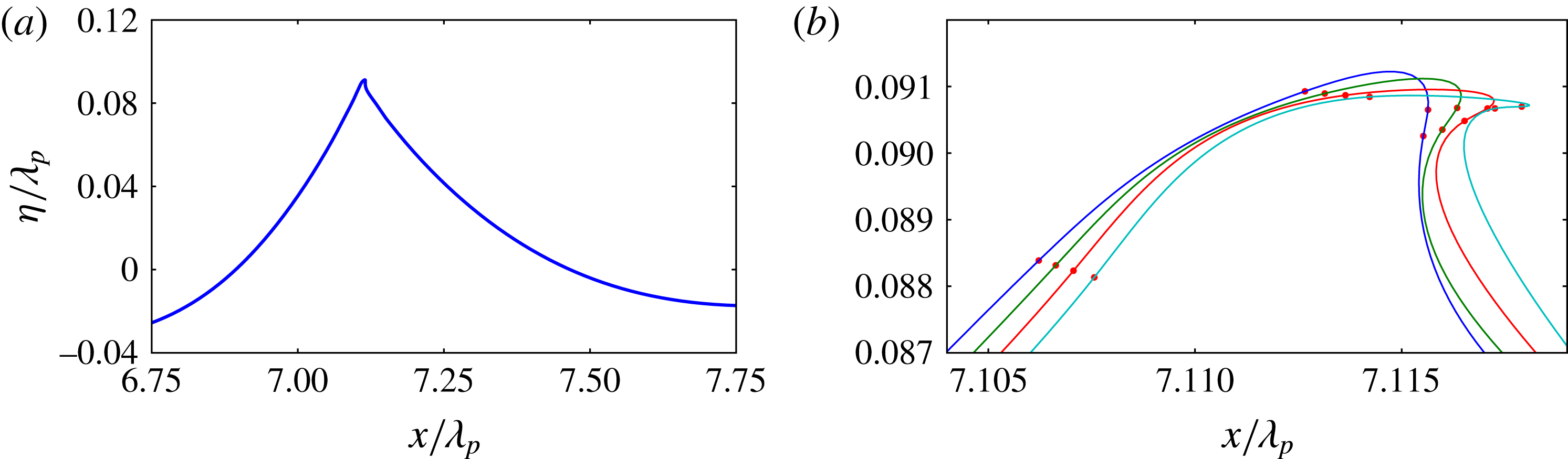
Evolution details of the initiation of crest roll-over at the tallest crest of a 2D C3N5 deep water wave packet undergoing weak breaking. The sequence of local crest surface profiles corresponding to the incipient breaking wave in (a) is shown in (b), starting after the appearance of the vertical tangent on the forward face. The crest tip moves from left to right. The small solid circles indicate the computational nodes. Details of the splined curves are given in § 3.2.

Three-dimensional simulations, with
 $x$
as the main direction of propagation,
 $y$
the transverse horizontal direction and
 $z$
the vertical direction, were run using mainly 16 nodes per wavelength. The insensitivity of the results to the resolution was established by a subset of runs using 32 nodes per wavelength. The number of nodes in the
 $y$
- or
 $z$
-direction was adjusted to keep the boundary element aspect ratio close to 1. Figure 1(a) shows a typical elevation profile of a gently breaking 2D C3N5 deep water wave packet (see § 3.1 and tables 1 and 2 captions for run code terminology) just after exceedance of our breaking onset threshold. This case is discussed in detail in § 5.4 and shown in figure 7(b,d). Figure 1(b) shows the sequence of elevation profiles of this overturning wave crest at incremental time steps. It highlights the ensuing development of the crest tip jet following the occurrence of a vertical tangent on the forward face, confirming the overturning capability of WSIM.
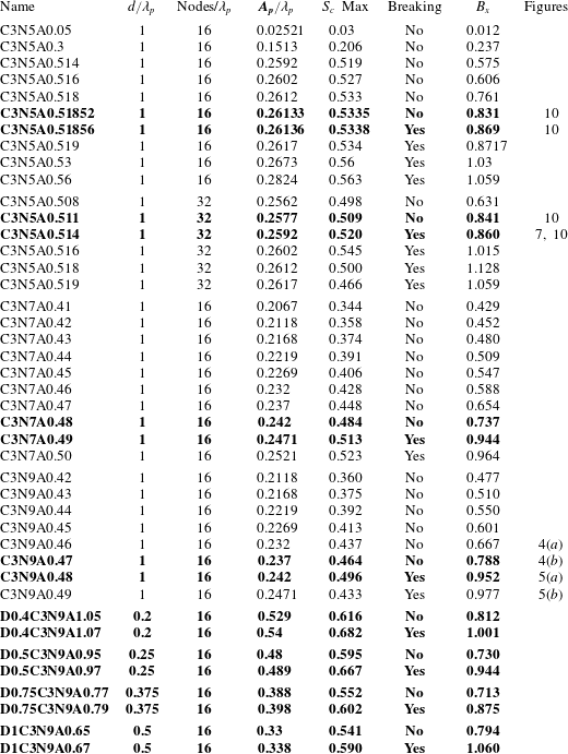
Results for each simulated 2D wave group within the several ensembles listed, showing whether recurrent or breaking, with the maximum steepness
 $S_{c}$
and maximum
 $B_{x}$
. For each group name, the N[I] in the group name denotes the number of waves [I] in the temporal packet,
 $A_{p}/\unicode[STIX]{x1D706}_{p}$
is the paddle amplitude and
 $d/\unicode[STIX]{x1D706}_{p}$
is the still water depth relative to the wavelength. The D0.P prefix indicates the relative depth, where
 $\text{P}=2d/\unicode[STIX]{x1D706}_{p}$
. The bold entries bracket the transition between the maximum recurrence and marginal breaking case for each group type.

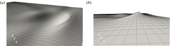
Figure 2 shows a typical simulation using 16 nodes per wavelength. It illustrates the breaking initiation of the crest of a 3D converging deep water chirped wave packet with five waves in the temporal group. Even though each cell is represented by a flat quadrangle in the visualisations in figure 2, bicubic and fourth-order basis polynomials were used respectively for the physical variables and the geometry, providing second-order curvature discretisation.
Each breaking case we investigated conforms to this generic systematic progression (exceeding the breaking threshold, subsequent vertical tangent on forward face of crest and formation of initial crest tip jet). The numerics handles this smoothly, with the code stopping when the boundary elements at the crest tip jet become enmeshed. However, this occurs well beyond the exceedance of the breaking onset threshold and has no impact in determining this threshold. This is described in § 3.4 and in greater detail in § A.3.
The mixed Eulerian–Lagrangian numerical scheme and the high nonlinearity of the waves make the free-surface mesh prone to distortion by the Lagrangian drift current. Extreme care was taken so that even at maximum recurrence, only a moderate Lagrangian drift was produced and the mesh did not deform significantly. An important benefit of the local Lagrangian drift is the clustering of the nodes around sharp crests.
Numerical wave tank simulation showing the initiation of breaking at the leading crest of a 3D converging C3N5 deep water wave packet as it propagates to the right. (a) The computational domain; (b) a zoomed-in view of the overturning crest. The simulation used 16 nodes per wavelength, a paddle amplitude of
 $A_{p}/\unicode[STIX]{x1D706}_{p}=0.2067$
and a linear focal distance of
 $x/\unicode[STIX]{x1D706}_{p}=5$
. The rectangular cells are artefacts of the visualisation.

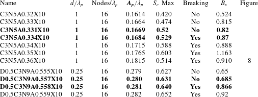
The same as table 1, but showing our results for the 3D runs. The D0.P prefix indicates the relative depth, where
 $\text{P}=2d/\unicode[STIX]{x1D706}_{p}$
, as for the 2D cases, and the X10 designation indicates focusing at approximately
 $x/\unicode[STIX]{x1D706}_{p}=5$
.

3.3 Scaling parameters in the numerical simulations
The numerical simulations use the following deep water (DW) non-dimensional parameter scalings: the reference time scale is based on the baseline frequency
 $\unicode[STIX]{x1D714}_{p}$
of the paddle; the corresponding linear dispersion reference length scale is the wavelength (
 $\unicode[STIX]{x1D706}_{p}$
) at the wavemaker (with corresponding wavenumber
 $k_{p}$
). The deep water dispersion relation imposes a gravitational acceleration
 $g_{DW}=2\unicode[STIX]{x03C0}$
and a reference linear phase speed
 $c_{DW}=1$
. With these scalings, results have been produced for depth to wavelength ratios
 $(d/\unicode[STIX]{x1D706}_{p})$
in the interval
 $[0.2,1]$
.
3.4 Numerical convergence
This research aims to identify a criterion that can robustly predict whether growing 2D or 3D carrier waves in evolving wave groups will attain their maximum steepness without breaking (recurrent waves) or proceed to break, with overturning crests. To achieve this aim, the weakest form of breaking, marginal breaking, was computed and compared with the corresponding maximum recurrent case. We carried out a detailed sensitivity study that demonstrates convergence of the NWT model even for such low-intensity breaking. Sensitivity tests were performed for one 2D ensemble, C3N5, using the two different resolutions described above (16 and 32 nodes per wavelength). We confirmed that both resolutions share the initial stage of breaking onset, confirmed by the occurrence of a vertical forward face segment and a multiple-valued free surface. While some minor differences were seen between the different resolutions, the numerical convergence of the computed breaking parameter is discussed in detail in § A.3, where it is established that the resolution of 16 nodes per wavelength suffices to robustly quantify the breaking onset threshold.
4 Analysis of simulation data using previous breaking criteria
The recent review paper of Perlin et al. (Reference Perlin, Choi and Tian2013) provides a detailed analysis of the different classes of proposed breaking criteria. Shortcomings have been identified in each of the criteria proposed to date. In the present study, several of these breaking criteria were also investigated using our simulation data and their validity evaluated.
4.1 Geometrical criteria
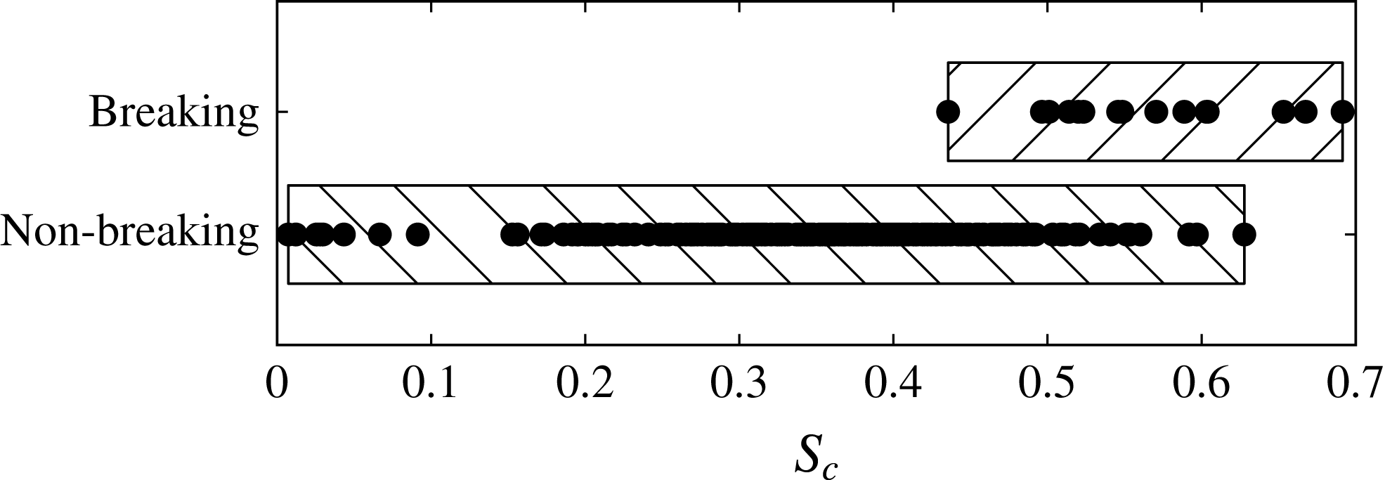
As reported in Perlin et al. (Reference Perlin, Choi and Tian2013), geometric threshold criteria were not found to be robust (in the generic sense) in previous observational studies. Figure 3 provides an overview of the performance of the steepness criterion for breaking onset for the present data set. It shows the distribution of the maximum local crest steepness
 $S_{c}=\unicode[STIX]{x03C0}a/\unicode[STIX]{x1D706}_{c}$
of each of the recurrent or breaking wave packets. Here,
 $a$
is the crest amplitude and
 $\unicode[STIX]{x1D706}_{c}$
is the horizontal extent, measured between the wave profile zero up and down crossings that span the crest (Banner et al.
Reference Banner, Barthelemy, Fedele, Allis, Benetazzo, Dias and Peirson2014). Our results confirm previous findings that breaking onset cannot be discriminated by the steepness criterion since some breaking crest cases have a significantly lower
 $S_{c}$
than recurrent waves.
Distribution of local crest maximum steepness
 $S_{c}$
partitioned according to breaking or recurrent events for all the C3 wave packets investigated in this study. One can note the extensive
 $S_{c}$
range shared by non-breaking and breaking waves.

4.2 Kinematic criteria
As described in Perlin et al. (Reference Perlin, Choi and Tian2013), various kinematic breaking criteria have been proposed. We note that Stansell & MacFarlane (Reference Stansell and MacFarlane2002) and Kurnia & van Groesen (Reference Kurnia and van Groesen2014) mentioned a variety of purely kinematic criteria (ratio of fluid speed to wave speed larger than 0.7, 0.8 and 1) which are embraced by our findings in the present paper. However, there is no guidance as to the universality of the detection of breaking onset.
Recently, Banner et al. (Reference Banner, Barthelemy, Fedele, Allis, Benetazzo, Dias and Peirson2014) investigated the influence of unsteadiness in dispersive wave packets, based on results from numerical simulations and complementary laboratory and ocean tower measurements. Their study highlighted the existence of a significant kinematic/geometric phenomenon attributable to the extra degrees of freedom in such unsteady wave packets. This results in an additional generic oscillatory crest/trough leaning mode characterising the carrier wave evolution. For focusing deep water wave packets, this is manifested as a systematic crest speed slowdown of approximately 20 % of the linear phase velocity, reconciling why their breaking crests are observed to have initial speeds typically 20 % lower than the corresponding linear phase speed for that wavelength. The source of the crest slowdown mechanism was investigated in Banner et al. (Reference Banner, Barthelemy, Fedele, Allis, Benetazzo, Dias and Peirson2014), Fedele (Reference Fedele2014) and Barthelemy et al. (Reference Barthelemy, Banner, Peirson, Dias and Allis2015). Most significantly, it determines the underlying crest motion from which the breaking onset initiates, which is a key element in our new breaking framework.
4.3 Dynamical criteria
Dynamical criteria link the physics of breaking onset to the energy fluxes associated with the underlying unsteady wave group structure. Conceptually, the rate of convergence of the intragroup energy flux exceeds a local stability level at a particular crest, which triggers this crest to break. The highly nonlinear, spatially non-uniform and unsteady nature of the flow field makes rigorous analysis difficult. One of the key results in § 1 describing dynamical breaking criteria was the proposition that breaking onset is initiated when the crest particle speed exceeds the linear group speed (Tulin & Landrini Reference Tulin and Landrini2000). We were able to investigate this criterion for chirped nonlinear wave packets for a range of depth conditions, including 3D cases. However, based on our findings in § 6 below, our results do not support their proposed criterion.
We also revisited the wave-group-related energy flux approach investigated in the modelling study of Song & Banner (Reference Song and Banner2002) and validated observationally in Banner & Peirson (Reference Banner and Peirson2007). This approach examined the possibility of a generic local parametric energy convergence rate for 2D wave groups following the wave group maximum (see § 3.3 in Perlin et al. Reference Perlin, Choi and Tian2013). Further support was recently reported for 2D breaking onset by Derakhti & Kirby (Reference Derakhti and Kirby2016) (§ 1). However, two factors motivated our present search for an alternative breaking criterion based on an energy convergence rate threshold.
First, our present study found that 2D and 3D breaking onset behaviour did not closely match the 2D threshold growth rate proposed by Song & Banner (Reference Song and Banner2002). For both 2D and 3D cases in our study, the computed local carrier wavenumber used in constructing the Song & Banner (Reference Song and Banner2002) growth rate did not increase monotonically as the wave steepened, contrary to the analysis of Song & Banner (Reference Song and Banner2002). This departure was also observed experimentally in § 6.3 of Allis (Reference Allis2013). As a result, the diagnostic growth rate trajectory departed significantly from the results reported in Song & Banner (Reference Song and Banner2002). Second, the approach of Song & Banner (Reference Song and Banner2002) requires tracking, for any given crest, of the space–time locus of its maximum elevation for at least two cycles prior to its reaching its ultimate maximum (either the recurrence maximum or the onset of breaking). Aside from its measurement complexity, this approach becomes tenuous for cases when more rapid approach to breaking onset occurs with fewer than three growth cycles. These factors underpinned our systematic search for a less restrictive energy flux-based breaking criterion.
5 New breaking criterion based on the local energy flux velocity
Conceptually, the onset of breaking may be regarded as the inability of the waveform to accommodate a local wave energy flux which exceeds that in the corresponding maximum recurrent case. It is observed that breaking of the dominant waves typically occurs at the crest of the tallest dominant wave within a group, showing the preferred crest localisation of the phenomenon. This is consistent with the open ocean observations of Holthuijsen & Herbers (Reference Holthuijsen and Herbers1986). Excess local wave energy flux can arise from a variety of sources, such as intrawave energy exchanges, wind–wave exchange, geometrical and temporal 3D wave focusing, wave–current interactions, among others. For the present focus on unforced water wave groups, we hypothesise that the same breaking onset physics could apply whether the wave group is evolving in deep water or in intermediate water depth. The shortcomings of the various criteria described above led us to focus on the role of excess wave energy flux as the underpinning element of a generic breaking criterion. Section 2.3 of Phillips (Reference Phillips1977) introduces the wave energy flux vector and its local conservation equation (2.3.2).
5.1 Energy flux considerations in nonlinear wave groups
The mechanical energy balance equation relates the local rate of change of the energy density
 $E$
,
 $$\begin{eqnarray}E=\unicode[STIX]{x1D70C}g(z-z_{0})+{\textstyle \frac{1}{2}}\unicode[STIX]{x1D70C}\Vert \boldsymbol{u}\Vert ^{2},\end{eqnarray}$$
to the divergence of the local energy flux
 $\boldsymbol{F}$
,
 $$\begin{eqnarray}\boldsymbol{F}=\boldsymbol{u}\left((p-p_{0})+\unicode[STIX]{x1D70C}g(z-z_{0})+{\textstyle \frac{1}{2}}\unicode[STIX]{x1D70C}\Vert \boldsymbol{u}\Vert ^{2}\right),\end{eqnarray}$$
where
 $p$
is the pressure,
 $p_{0}$
is the ambient pressure above the surface (taken as zero without loss of generality),
 $\Vert \boldsymbol{u}\Vert$
is the fluid speed,
 $g$
is gravitational acceleration,
 $z$
is the vertical coordinate and
 $z_{0}$
is the datum.
With the above definitions, equation (3.6.14) in Phillips (Reference Phillips1977) shows the conservation law for the depth-integrated energy. Based on (3.6.14), we performed an analysis of the crest behaviour of the depth-integrated energy density, depth-integrated energy flux and its gradient at maximal focusing for representative nonlinear wave packets. We investigated examples of chirped packets with different numbers of carrier waves. Our aim was to determine whether breaking onset provides a distinctive signature within the depth-integrated energy context. We concluded that this depth-integrated approach obscures this apparently highly localised crest instability. To detect the transition to breaking above the background wave energy, it became evident that a local energy flux analysis in the neighbourhood of the crest was needed. This is described in the following section.
5.2 Breaking criterion based on the local energy flux velocity
For the present purposes, in an inertial frame of reference, the local energy density conservation law (Phillips Reference Phillips1977, equation (2.3.2))] takes the Eulerian form:
 $$\begin{eqnarray}{\displaystyle \frac{\unicode[STIX]{x2202}E}{\unicode[STIX]{x2202}t}}+\unicode[STIX]{x1D735}\boldsymbol{\cdot }(\boldsymbol{u}(E+p))=0.\end{eqnarray}$$
From (5.3), in an inertial frame of reference, the energy flux velocity is seen to be the fluid velocity
 $\boldsymbol{u}$
. However, to gain a refined understanding of the energy flux to the tallest crest in an evolving nonlinear wave packet, the corresponding conservation equation for a control volume moving with the (unsteady) crest velocity
 $\boldsymbol{c}$
has the form (Tulin Reference Tulin2007, equation (1.2))
 $$\begin{eqnarray}{\displaystyle \frac{D_{c}E}{\text{D}t}}+\unicode[STIX]{x1D735}\boldsymbol{\cdot }((\boldsymbol{u}-\boldsymbol{c})E+\boldsymbol{u}p)=0,\end{eqnarray}$$
where
 $D_{c}E/\text{D}t=\unicode[STIX]{x2202}E/\unicode[STIX]{x2202}t+\boldsymbol{c}\boldsymbol{\cdot }\unicode[STIX]{x1D735}E$
is the rate of change following the crest. Along the unforced free surface, (5.4) reduces to
 $$\begin{eqnarray}{\displaystyle \frac{D_{c}E}{\text{D}t}}+\unicode[STIX]{x1D735}\boldsymbol{\cdot }((\boldsymbol{u}-\boldsymbol{c})E)=0,\end{eqnarray}$$
which shows that
 $(\boldsymbol{u}-\boldsymbol{c})$
is the relevant flux velocity transporting energy to the growing crest.
These theoretical aspects, taken in context with allied observational and computational considerations, motivated our investigation of the behaviour of the local energy flux
 $\boldsymbol{F}$
in relation to the local energy density
 $E$
in the neighbourhood of the wave crest in the fixed frame of reference. Here, (5.3) can be used, along with the incompressibility condition
 $\unicode[STIX]{x1D735}\boldsymbol{\cdot }\boldsymbol{u}=0$
, to quantify the ratio
 $\boldsymbol{F}/E$
as follows:
 $$\begin{eqnarray}\boldsymbol{F}/E=\boldsymbol{u}(E+p)/E.\end{eqnarray}$$
On the free surface,
 $\boldsymbol{F}/E$
reduces to the surface fluid velocity
 $\boldsymbol{u}$
. Given the intrinsic relevance of the crest velocity
 $\boldsymbol{c}$
highlighted above, we adopt
 $\boldsymbol{c}$
as the natural normalising velocity for the flux ratio in (5.6) and introduce a breaking onset threshold parameter
 $\boldsymbol{B}$
as
 $$\begin{eqnarray}\boldsymbol{B}=\boldsymbol{F}/(E\Vert \boldsymbol{c}\Vert ).\end{eqnarray}$$
The above analysis indicates that the crest speed is a key variable in the breaking onset threshold parameter
 $\boldsymbol{B}$
, as mentioned above in § 4.2. The recent study by Banner et al. (Reference Banner, Barthelemy, Fedele, Allis, Benetazzo, Dias and Peirson2014) and Barthelemy et al. (Reference Barthelemy, Banner, Peirson, Dias and Allis2015) provided new insights into crest speed behaviour in the unsteady evolution of nonlinear dispersive water wave packets. Specifically, every wave in an unsteady dispersive wave group experiences a dynamic leaning cycle. Crests and troughs enter at the rear of the wave group first leaning forward, then transitioning through symmetry, and subsequently leaning backward as they propagate towards the front of the wave group. In deep water, this leaning cycle creates a systematic crest slowdown to approximately 80 % of the linear phase velocity
 $c_{0}$
, with only a weak dependence on the (local) steepness of the crest or trough. Here,
 $c_{0}$
is the linear phase speed corresponding to the peak frequency
 $\unicode[STIX]{x1D714}_{0}$
of the local frequency spectrum of the wave packet, assuming the linear dispersion relation. However, in shallower water depth, the waves are less dispersive and the crest slowdown effect reduces, with crest speeds approaching the phase speed. As will be seen below, use of the crest speed
 $c$
underpins our key finding of a robust breaking onset threshold.
During the crest life cycle, the local energy flux speed becomes maximal near the crest point, as will be shown below. Since
 $\boldsymbol{F}$
and
 $\boldsymbol{c}$
are vectors, we have two convenient choices to construct their ratio, either to project along the wave propagation direction (taken here as the
 $x$
-direction) or to use norms. This leads to the two following dimensionless quantities:
 $$\begin{eqnarray}B_{x}=F_{x}/(Ec_{x})\quad \text{or}\quad B=\Vert \boldsymbol{F}\Vert /(E\Vert \boldsymbol{c}\Vert ).\end{eqnarray}$$
Since it is found that there is no difference between the two ratios when the crest reaches its maximum (the vertical components of the flux and of the crest speed vanish), we only explore the validity of
 $B_{x}$
as a breaking threshold parameter that embraces wave kinematics and energetics. As discussed in detail below, the distributions of
 $E$
,
 $\boldsymbol{F}$
and
 $\boldsymbol{B}$
provide key insights into the surface and subsurface manifestation of breaking onset. We note that the bottom depth topography does not play an explicit role in the above discussion of our breaking onset threshold.
5.3 Breaking onset threshold and its surface signature
Here, we report results investigating our breaking onset criterion in terms of a parametric threshold band, as described in detail in § 5.1. This band is bounded below by a maximal non-breaking condition and above by a marginal breaking condition for individual waves in the local carrier wave system. Fortuitously, the threshold parameter specified in (5.8) has a simple signature along the free surface.
As explained above, the pressure
 $p$
at the free surface is assumed to be constant and is taken as zero without loss of generality. The energy flux velocity then reduces to the fluid particle velocity, and our proposed breaking criterion for
 $B_{x}$
, based on the excess energy flux of the marginal breaking case over the corresponding maximal recurrent case, remarkably reduces to a kinematic criterion at the free surface,
 $$\begin{eqnarray}B_{x}=F_{x}/Ec_{x}=u_{x}/c_{x}>\text{threshold}.\end{eqnarray}$$
Accordingly, we performed a suite of numerical simulations to investigate the behaviour of
 $B_{x}$
at the free surface, as defined in (5.9). As described in detail below, the onset of breaking was found to occur when
 $0.85<B_{x}<0.86$
for our entire ensemble of numerical experiments addressing 2D and 3D deep water and intermediate depth cases over flat bottom topography. In addition to this remarkable result, it is noteworthy that after factoring out the reduced crest speed in deep water (
 ${\approx}0.8c_{0}$
), this corresponds to
 $u/c_{0}\approx 0.68$
, which is well below the often-quoted classical kinematic breaking criterion
 $u/c_{0}>1$
.
With regard to 3D breaking validation, energy flux is a vector quantity and our criterion is able to accommodate the additional lateral energy flux in 3D converging cases. Our 3D numerical simulations comprise two representative cases with different bandwidths and water depths, and the most severe lateral convergence (focal distance
 ${\approx}5$
carrier wavelengths): a deep water C3N5 case with five waves and an intermediate depth
 $(d/\unicode[STIX]{x1D706}_{p}=0.25)$
C3N9 case with nine waves.
While the surface-based
 $B_{x}$
criterion provides the most convenient operational breaking onset threshold criterion, the associated subsurface distribution of
 $B_{x}$
, defined in (5.8), was also investigated, and representative results are reported below in § 5.4. The discussion now addresses the generic behaviour of
 $B_{x}$
at the free surface.
Representative behaviour of
 $B_{x}$
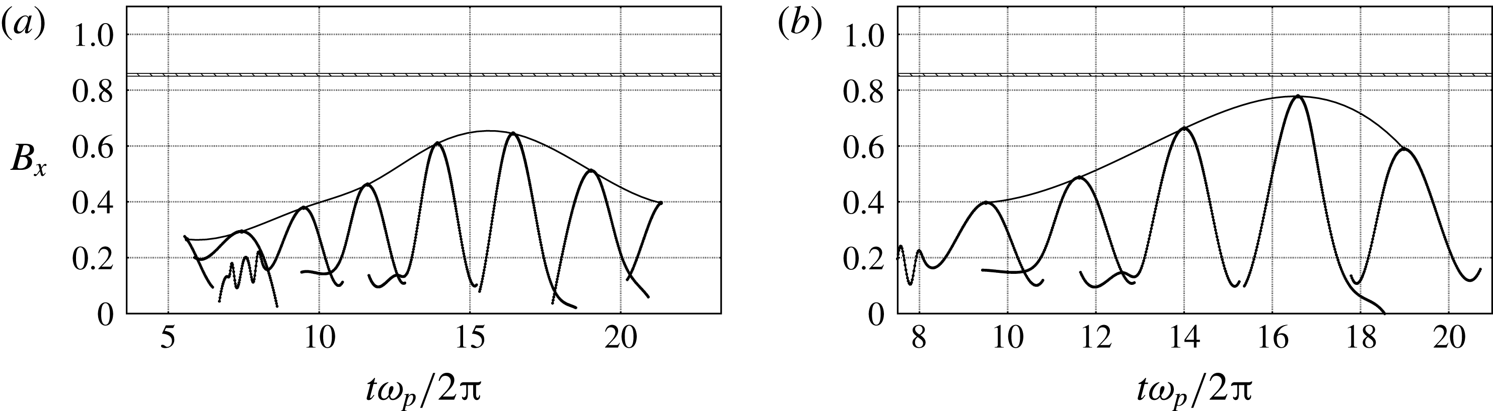
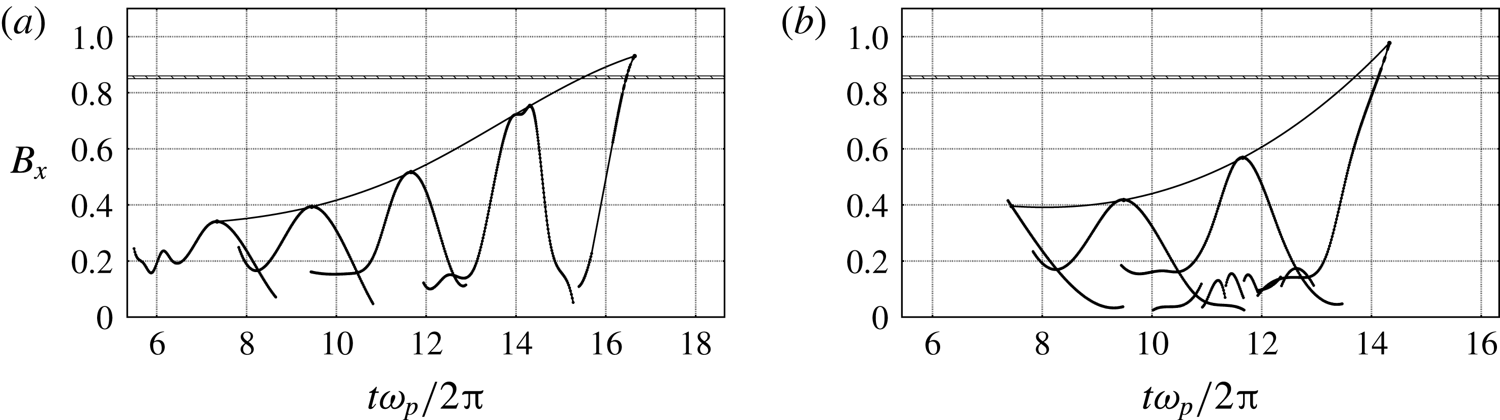
is shown in figures 4(a,b) and 5(a,b), which show the time evolution of the breaking parameter
 $B_{x}$
following the peak of each crest during the group propagation. The two cases illustrate near-maximum recurrence and marginally breaking behaviour of 2D deep water packets. The hatched zone is the identified threshold level of 0.85–0.86 determined by our entire ensemble of simulations, above which all crests proceeded to break. In the near-maximum recurrence case (figure 5
b), the trajectories never cross the hatched zone, in contrast to figure 5(a), which shows the marginal breaking case of the same wave group class, where the trajectory of
 $B_{x}$
clearly crosses the threshold.
Breaking criterion
 $B_{x}$
as a function of time for recurrent C3N9 2D chirped wave packets. Each trajectory curve shows the time evolution of the breaking parameter
 $B_{x}$
following each carrier wave crest maximum during the packet evolution as it grows, attains its maximum steepness without breaking and then decays. (a) Paddle amplitude
 $A_{p}/\unicode[STIX]{x1D706}_{p}=0.232$
. (b) Paddle amplitude
 $A_{p}/\unicode[STIX]{x1D706}_{p}=0.237$
.

Breaking parameter
 $B_{x}$
as a function of time for breaking C3N9 2D chirped wave packets. Each trajectory curve show the time evolution, up to breaking onset, of the breaking parameter
 $B_{x}$
following each carrier wave crest maximum during the packet evolution. The trajectory of the breaking crest clearly crosses the proposed breaking onset threshold
 $[0.85,0.86]$
. (a) Paddle amplitude
 $A_{p}/\unicode[STIX]{x1D706}_{p}=0.242$
. (b) Paddle amplitude
 $A_{p}/\unicode[STIX]{x1D706}_{p}=0.247$
.

In these examples, the computed spline passing through all of the local crest maxima also shows their longer-term evolution trajectory. In the breaking case, this spline crosses the hatched breaking threshold zone before breaking subsequently initiates, providing advance warning of up to half of a carrier wave period. This behaviour is representative of all investigated breaking cases.
Our key results for the proposed breaking onset threshold are based on
 $B_{x}$
derived from the ensemble of systematic numerical simulation cases shown in table 1. For each generic packet type, the results are ordered according to increasing paddle amplitude, with the transition from maximal non-breaking to marginal breaking highlighted. The C3N5 results at the top of the table confirm the insensitivity of the results to the resolution, as discussed in detail in § A.3 of the appendix.
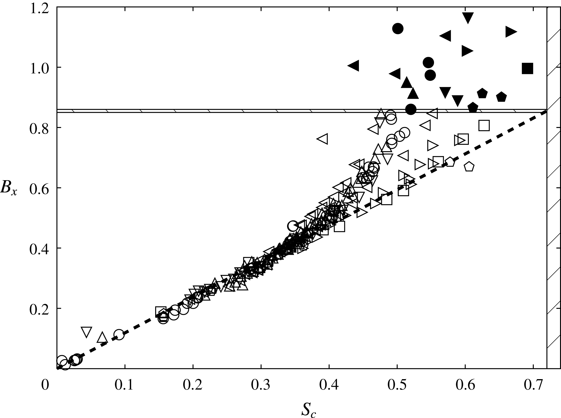
Breaking parameter
 $B_{x}$
plotted against local steepness
 $S_{c}$
at the maximum crest tip elevation, obtained by tracking
 $B_{x}$
for every crest in each packet evolution documented in tables 1 and 2. Recurrent cases are determined at their maximum height and breaking crests when their vertical faces first appear. The horizontal hatched zone at
 $0.85<B_{x}<0.86$
is the threshold that segregates breaking from non-breaking cases; the vertical hatched zone
 $S_{c}>0.72$
is the deep water Stokes limit. Hollow symbols represent recurrent crests and solid symbols represent breaking crests. The wave group families are labelled as follows: circles, C3N5 2D deep water; downward-pointing triangles, C3N5 3D deep water; upward-pointing triangles, C3N7 2D deep water; leftward-pointing triangles, C3N9 2D deep water; rightward-pointing triangles, C3N9 2D
 $0.2<d/\unicode[STIX]{x1D706}_{p}<1$
; squares, C3N9 2D
 $d/\unicode[STIX]{x1D706}_{p}=0.2$
; pentagons, C3N9 3D
 $0.25\leqslant d/\unicode[STIX]{x1D706}_{p}<1$
.

Figure 6, the key figure in this paper, provides a comprehensive summary of the performance of the breaking onset threshold for the present data set. We track the magnitude of the breaking onset parameter
 $B_{x}$
for each crest tip in the packet during the evolution. We record its value and corresponding local steepness
 $S_{c}$
at its maximum elevation for recurrent crests, or when the vertical forward face segment first appears for breaking crests. Figure 6 displays the ensemble of these maximal
 $(B_{x},S_{c})$
values for all of the different packet case evolutions investigated in tables 1 and 2. Both 2D and 3D deep and intermediate water depth cases are included. The vertical hatched zone on the right represents the classical Stokes local steepness limit expressed in terms of
 $S_{c}$
rather than
 $ak$
. The horizontal hatched zone
 $[0.85<B_{x}<0.86]$
is the breaking threshold determined from our ensemble of numerical simulations. This figure highlights two significant findings. The major finding is the discovery of a clear separation between recurrent and breaking crests. For recurrence cases, our proposed breaking onset parameter
 $B_{x}$
is always less than 0.85, below which crests were never found to break. However,
 $B_{x}$
is always greater than 0.86 when breaking occurs. This identifies the breaking onset threshold zone for
 $B_{x}$
as
 $[0.85,0.86]$
.
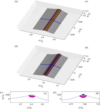
Contours of the breaking criterion
 $B_{x}$
for the 2D C3N5A0.514 breaking wave case. The regions are colour-coded as follows: red,
 $B_{x}>0.85$
; green,
 $0.7<B_{x}<0.85$
; blue,
 $0.6<B_{x}<0.7$
; yellow,
 $0.5<B_{x}<0.6$
; magenta,
 $0.4<B_{x}<0.5$
; white,
 $B_{x}<0.4$
. (a) Colour-coded zones of the breaking parameter
 $B_{x}$
on the free surface at
 $t=13.85$
. The blue line is the location of the slice seen in (c). (b) The same as (a) at
 $t=14.41$
. The blue line is the location of the slice seen in (d). (c) Colour-coded cross-section within the slice
 $y=0$
shown in (a). (d) Colour-coded cross-section within the slice
 $y=0$
shown in (b).

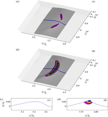
The same as figure 7 but for the 3D C3N5A0.36X10 breaking wave case. (a) Colour-coded zones of the breaking parameter
 $B_{x}$
on the free surface at
 $t=12.45$
. The blue line is the location of the slice seen in (c). (b) The same as (a) at
 $t=12.84$
. The blue line is the location of the slice seen in (d). (c) Colour-coded cross-section within the slice
 $y=0$
shown in (a). (d) Colour-coded cross-section within the slice
 $y=0$
shown in (b).

The other finding concerns the relationship between crest steepness at maximum wave height and breaking onset. Once again, it is seen that crest steepness is clearly not a threshold variable that is able to discriminate between breaking and recurrence. This is evident as the local steepness for breaking crests can be lower than the local steepness of recurrent evolution cases for a given depth (or
 $kd$
). We note that a straight line can be drawn between
 $(0,0)$
and
 $(S_{c_{max}},0.855)$
. All of the symbols for the individual crests are closely aligned at low steepness and then a departure from this trend occurs due to nonlinearities. The
 $B_{x}$
parameter then grows faster than the steepness. This transition occurs at higher steepness levels in intermediate water depth than in deep water. The limiting case for shallow water conditions (
 $kd\rightarrow 0$
) seems to converge towards the deep water Stokes limiting steepness. Tables 1 and 2 summarise respectively the properties and results of the 2D and 3D cases processed for this study.
It is worth noting that the 3D simulations, while fully supporting our breaking onset criterion, exhibit a much higher sensitivity for the shallow depth case to very small increments in the paddle amplitude approaching maximum recurrence. Approaching the recurrence maximum, an increase of only 0.2 % in the paddle amplitude resulted in a change in
 $B_{x}$
of approximately 25 %. Such sensitivity challenges the numerical precision of the code if further refinement is sought.
5.4 Subsurface energy flux considerations
The breaking parameter
 $B$
is based on the local wave energy flux
 $\Vert \boldsymbol{F}\Vert$
normalised by the local wave energy density
 $E$
and the wave crest speed
 $\Vert \boldsymbol{c}\Vert$
, defined at the maximum elevation of the crest. The energy density and the energy flux are both well-behaved field quantities and reach their maximum at the crest point maximum. Because these quantities include the potential energy, their value is defined relative to an arbitrary constant, the datum
 $z_{0}$
. The total energy
 $E=\unicode[STIX]{x1D70C}g(z-z_{0})+\unicode[STIX]{x1D70C}u^{2}/2$
may vanish locally, depending on the choice of the datum
 $z_{0}$
. Accordingly, to avoid spurious singularities of
 $\boldsymbol{B}$
and their effect on the
 $\boldsymbol{B}$
distribution arising within the flow domain, the datum level
 $z_{0}$
needs to be chosen outside the flow domain. We chose the datum as twice the depth of the flow domain, and verified that the subsurface
 $\boldsymbol{B}$
distributions were insensitive to
 $z_{0}$
lower than this.
The breaking onset threshold parameter
 $\boldsymbol{B}$
exists both on the surface and in the interior of the wave domain. It can be computed for maximum recurrent crests and for crests evolving to breaking, up to the point of breaking onset. Figures 7 and 8 highlight key properties of interest respectively of 2D and 3D waves evolving towards breaking. In these figures, each spatial snapshot (A) and (B) shows the
 $B_{x}$
distribution at two different evolution times of the wave packets. The first two panels (a) and (b) are colour-coded representations showing contours of the breaking onset parameter (
 $B_{x}$
) on the crest surface (figures 7
a,b and 8
a,b). The other panels (figures 7
c,d and 8
c,d) are vertical plane cross-sectional slices along the symmetry axis of the crest (blue lines in figures 7
a,b and 8
a,b).
These plots highlight the localisation of the
 $B_{x}$
maximum at the crest tip of the tallest wave, which is similar for the 2D and 3D cases. Of further interest is the spatial extent of the region involved in a breaking onset event. Based on the
 $B_{x}$
parameter threshold, the horizontal extent of the zone where
 $B_{x}$
values exceed 50 % of the breaking onset threshold is close to 10 % of the wavelength, within the already narrow crest region.
Observational validation of our new breaking criterion is challenging, due to its spatial localisation within a rapidly evolving compact zone. Its horizontal extent where
 $B_{x}$
exceeds the breaking threshold is only approximately 3 % of the wavelength. Since the non-dimensional wave crest speed is close to 0.85 at breaking, a fixed probe will reside in this zone for only approximately 0.04 non-dimensional time units. Accurate determination of the rapidly evolving crest speed and its associated surface fluid speed is a demanding measurement. Careful physical experiments are needed to validate these new findings. Such studies have been undertaken and the results reported in Saket et al. (Reference Saket, Peirson, Banner, Barthelemy and Allis2017) for 2D waves in deep water and in Saket et al. (Reference Saket, Peirson, Banner and Allis2018) for intermediate water depths. These studies encompassed different classes of nonlinear deep water and intermediate depth wave groups, for a range of group bandwidths. The influence of wind forcing was also investigated for deep water cases. Their results show agreement with our proposed breaking onset threshold criterion to within 2.5 %, which is close to the experimental error bounds.
For comparison with our 3D simulation results, chap. 6 in Saket (Reference Saket2017) presents companion observational results for 3D chirped (and also modulationally unstable) deep water wave packets with both strong and the most severe lateral focusing. These results offer strong support for our 3D simulation results, with an enhanced sensitivity to paddle amplitude observed in
 $B_{x}$
values for carrier wave crests approaching maximum recurrence.
It is interesting to note that the spatial regions where
 $B_{x}$
becomes appreciable in 2D and 3D breaking waves have approximately the same vertical extent, but the surface distribution of
 $B_{x}$
differs considerably. For 3D converging waves, the maximal values are positioned on side lobes off the symmetry axis. As the wave steepens, these lobes converge towards the symmetry axis, with
 $B_{x}$
becoming maximal on the symmetry axis where the wave breaks. In contrast, 2D breaking waves have an almost constant spanwise distribution of
 $B_{x}$
values, with only minor variations found where the loci of maximum
 $B_{x}$
values are on either side of the symmetry axis.
5.5 Possible influence of surface tension on the energy fluxes
The above investigation was carried out neglecting surface tension effects, which may become significant in zones of higher surface curvature. We assessed the validity of this assumption at the crest point of a 2D C3N5 wave transitioning through the
 $B_{x}=[0.85,0.86]$
breaking threshold with a wavelength of order 1 m. We found the radius of curvature
 $R=(1+(\unicode[STIX]{x1D701}^{\prime })^{2})^{3/2}/\unicode[STIX]{x1D701}^{\prime \prime }\approx 0.01$
, where
 $z=\unicode[STIX]{x1D701}$
specifies the free surface. The corresponding non-dimensional water-side pressure increment
 $\unicode[STIX]{x1D6FF}p=\unicode[STIX]{x1D70E}/\unicode[STIX]{x1D70C}R\approx 0.008$
is to be compared in the Bernoulli equation with the non-dimensional kinetic energy
 $KE=u^{2}/2\approx 0.3$
and non-dimensional potential energy
 $PE=g\unicode[STIX]{x1D701}\approx 0.58$
for the datum taken at
 $z_{0}=0$
.
Thus, the maximum water-side pressure increment associated with surface tension is estimated to be approximately 2 orders of magnitude lower than the energies, and therefore makes negligible difference to the energy fluxes. Further, we note that the crest point curvature of our numerical wave profiles as they transition the breaking onset threshold, which is well in advance of visual crest overturning, is only approximately three times the observed crest curvature of
 $O(1~\text{m})$
wavelength laboratory waves just before they proceed to overturn (e.g. see Qiao & Duncan (Reference Qiao and Duncan2001), figure 5a).
For water waves with even shorter wavelengths, there is the potential for our proposed breaking onset threshold to be modified by the effects of surface tension. This will only be resolved through detailed investigation.
6 Comparison with previously proposed breaking onset criteria
Our results do not support the criterion described by Tulin & Landrini (Reference Tulin and Landrini2000), which links breaking onset to the crest fluid speed exceeding the linear group speed of the wave packet.
Based on our results, for deep water waves, their threshold is equivalent to
 $B_{x}=0.62$
, which signals breaking onset at a considerably lower value than our
 $B_{x}$
threshold. However, in § 5.4, we highlighted the very close agreement (within 2.5 %) between our
 $B_{x}$
threshold value and the measured threshold reported by Saket et al. (Reference Saket, Peirson, Banner, Barthelemy and Allis2017) and Saket et al. (Reference Saket, Peirson, Banner and Allis2018) for modulationally breaking deep water and intermediate water depth wave packets. Further, as reproduced in Saket et al. (Reference Saket, Peirson, Banner, Barthelemy and Allis2017), our very steep deep water recurrent waves routinely exceed the proposed group-velocity-based threshold of Tulin & Landrini (Reference Tulin and Landrini2000) without breaking. For intermediate water depth waves, as the linear group speed approaches the linear phase speed, closer agreement with the Tulin & Landrini (Reference Tulin and Landrini2000) result might result for a specific water depth/wavelength ratio.
Perlin et al. (Reference Perlin, Choi and Tian2013) cite two studies that carefully compare the highest water speeds with coincident wave speeds. Just prior to overturning, Perlin, He & Bernal (Reference Perlin, He and Bernal1996) found a ratio of maximum water speed to linear wave speed of 0.74 for a single case of deep water plunging breaking. For intermediate water depths, Chang & Liu (Reference Chang and Liu1998) found a ratio of maximum water speed to linear wave speed of 0.86 prior to breaking. However, as shown by Banner et al. (Reference Banner, Barthelemy, Fedele, Allis, Benetazzo, Dias and Peirson2014), there is a systematic slowdown of the crest point as it transitions through its local maximum, and this crest slowdown was not taken into account by these investigators. After the crest slowdown is taken into account, their measurements are consistent with our findings, as both investigations reported water speeds exceeding 0.85 of the crest speed at breaking onset, with subsequent water speeds exceeding wave speeds during the overturning breaking process.
Saket et al. (Reference Saket, Peirson, Banner, Barthelemy and Allis2017) summarised results from a suite of other investigations that compared crest water speed with crest speed just prior to breaking onset. The most important of these studies is the work of Stansell & MacFarlane (Reference Stansell and MacFarlane2002), whose findings were found to be consistent with the results of Saket et al. (Reference Saket, Peirson, Banner, Barthelemy and Allis2017) once plausible and appropriate corrections were made to the near-surface velocity structure reported by Stansell & MacFarlane (Reference Stansell and MacFarlane2002). A detailed analysis of this aspect is given on pp. 653–655 in Saket et al. (Reference Saket, Peirson, Banner, Barthelemy and Allis2017).
7 Discussion and conclusions
A new breaking onset threshold criterion based on energy flux considerations has been developed for water waves and its applicability investigated for chirped focusing wave groups in deep and intermediate water depths. Our investigation of extensive 2D cases and targeted 3D cases with the most severe lateral focusing found consistent outcomes. While the energy flux that initiates breaking arises from energy focusing within the whole wave group, we found that the initial instability occurs within a very compact region, approximately 3 % of the wavelength in horizontal extent, centred on the maximum wave crest.
We found that depth-integrated quantities were not able to detect the signature of breaking generically in the phase-resolved wave motion. A more localised examination of the flow near the free surface was necessary to detect the initiation of breaking and to find a consistent deterministic indicator. Our new breaking criterion is based on the strength of the local energy flux relative to the local energy density, normalised by the local crest speed. This non-dimensional parameter
 $\boldsymbol{B}$
, which reduces to
 $B_{x}$
at the crest point (here,
 $x$
is the direction of propagation), simplifies fortuitously for zero surface pressure. On the free surface, it reduces to a kinematic condition for the ratio of crest fluid speed to crest point speed.
For the condition of zero surface pressure forcing, our suite of numerical experiments using a significant range of chirped wave packets has shown that our new dynamically based breaking onset parameter
 $B_{x}$
has a generic threshold value computed to be in the range
 $[0.85,0.86]$
, above which any local crest will undergo breaking onset. This threshold band is applicable everywhere in the fluid domain and has important new consequences.
Surface projection of our criterion is needed to make comparisons with previously proposed kinematic criteria. When projected along the surface, our criterion predicts breaking onset considerably in advance of the kinematic breaking criterion, where breaking is associated with the crest fluid speed exceeding the crest point speed. For maximally steep non-breaking waves, the crest fluid speed cannot exceed 0.85 of the crest speed. When referenced to the linear wave speed
 $c_{0}$
, after factoring in the generic crest slowdown for focusing dispersive deep water wave packets for which
 $c\approx 0.8c_{0}$
(see §§ 4.2 and 5.2), our
 $B_{x}$
threshold predicts breaking onset for deep water waves when the crest fluid speed to linear phase speed ratio
 $u/c_{0}$
exceeds 0.68. In progressively shallower water depth conditions, the generic crest slowdown reduces (
 $c\rightarrow c_{0}$
) and
 $u/c_{0}$
increases towards
 $[0.85,0.86]$
. In any event, it is evident that our breaking onset threshold band, which follows from energy flux considerations, occurs well before the water speed outruns the crest speed.
Overall, remarkable robustness of this new breaking onset threshold was found for the diverse range of 2D and 3D chirped focusing wave packets on deep and intermediate depth flat bottom topography investigated in this study. The threshold is also consistent with the findings of available comparable experiments for wavelengths of
 $O(1~\text{m})$
(Saket Reference Saket2017; Saket et al.
Reference Saket, Peirson, Banner, Barthelemy and Allis2017, Reference Saket, Peirson, Banner and Allis2018). Further investigation is needed for shorter waves, when surface tension effects may become important, and also for other commonly encountered breaking wave scenarios, such as waves shoaling on inclined bottom topography, coalescing wave groups and waves on uniform and shear currents. For these scenarios, since there is no explicit dependence on water depth, mean current or energy convergence rate in our energy flux considerations (§ 5.1), we anticipate that our breaking onset threshold will be applicable.
Acknowledgements
Funding for this investigation was provided by the Australian Research Council under Discovery Project DP120101701. Also, M.L.B. acknowledges ongoing support from the US Office of Naval Research during this project. F.D. acknowledges partial support by the European Research Council (ERC) under the research project ERC-2011-AdG 290562-MULTIWAVE and Science Foundation Ireland under grant no. SFI/12/ERC/E2227. M.A. acknowledges funding by New Zealand Ministry of Business, Innovation and Employment under project CAFS1803. X.B. performed all aspects of the computations. M.B. coordinated the scientific effort in close collaboration with X.B., F.F., W.L.P., F.D. and M.A., with the forensics underpinning the discovery performed by X.B. and M.L.B. They drafted this paper, with significant technical and intellectual input on the analysis and interpretation of the results from W.L.P., F.F., F.D. and M.A.
Appendix A. Details of the numerical wave tank
A.1 The numerical wave tank
WSIM uses a mixed Eulerian–Lagrangian time-updating scheme for irrotational motion described by the velocity potential
 $\unicode[STIX]{x1D719}(\boldsymbol{x},t)$
in a Cartesian coordinate system
 $\boldsymbol{x}=(x,y,z)$
with constant pressure at the open water surface. Here,
 $z$
is the vertical upward direction and
 $z=0$
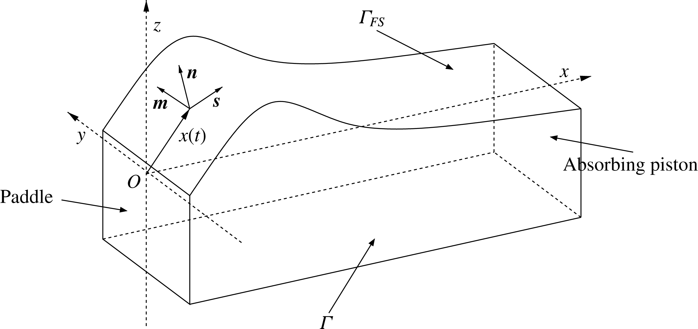
is the still water surface (figure 9).
Schematic (not to scale) of the WSIM simulation domain and nomenclature.

Fluid velocity is defined as
 $\boldsymbol{u}=\unicode[STIX]{x1D735}\unicode[STIX]{x1D719}=(u,v,w)$
. The continuity equation leads to the Laplace equation for the potential within the fluid domain
 $\unicode[STIX]{x1D6FA}(t)$
(A 1). The symbols
 $\unicode[STIX]{x1D6E4}$
and
 $\unicode[STIX]{x1D6E4}_{FS}$
are used to denote the entire domain boundary and the free surface respectively. The equations read as
 $$\begin{eqnarray}\displaystyle & \unicode[STIX]{x1D6FB}^{2}\unicode[STIX]{x1D719}=0\quad \text{on}~\unicode[STIX]{x1D6FA}, & \displaystyle\end{eqnarray}$$
 $$\begin{eqnarray}\displaystyle & \displaystyle \frac{\text{D}\boldsymbol{r}}{\text{D}t}=\boldsymbol{u}=\unicode[STIX]{x1D735}\unicode[STIX]{x1D719}\quad \text{on}~\unicode[STIX]{x1D6E4}_{FS}, & \displaystyle\end{eqnarray}$$
 $$\begin{eqnarray}\displaystyle & \displaystyle \frac{\text{D}\unicode[STIX]{x1D719}}{\text{D}t}=-gz+\frac{1}{2}\unicode[STIX]{x1D735}\unicode[STIX]{x1D719}\unicode[STIX]{x1D735}\unicode[STIX]{x1D719}-\frac{p_{0}}{\unicode[STIX]{x1D70C}}\quad \text{on}~\unicode[STIX]{x1D6E4}_{FS}, & \displaystyle\end{eqnarray}$$
 $$\begin{eqnarray}\displaystyle & \unicode[STIX]{x2202}_{n}\unicode[STIX]{x1D719}=0\quad \text{on}~\unicode[STIX]{x1D6E4}\backslash \unicode[STIX]{x1D6E4}_{FS}, & \displaystyle\end{eqnarray}$$
where
 $\boldsymbol{r}$
is the position vector of a fluid particle on the free surface,
 $g$
is the acceleration due to gravity,
 $p_{0}$
is the atmospheric pressure,
 $\unicode[STIX]{x1D70C}$
is the fluid density and
 $\text{D}/\text{Dt}(=\unicode[STIX]{x2202}/\unicode[STIX]{x2202}t+\unicode[STIX]{x1D735}\unicode[STIX]{x1D719}\boldsymbol{\cdot }\unicode[STIX]{x1D735})$
is the Lagrangian (or material) time derivative.
The free surface (domain
 $\unicode[STIX]{x1D6E4}_{FS}$
) is described by fully nonlinear kinematic (A 2) and dynamic (A 3) equations. Recent developments have implemented a 3D snake wave paddle at one vertical face of the domain, which is described subsequently. The far face of the numerical wave tank from the paddle has an absorbing beach which damps any incident wave energy, as described in Grilli & Horrillo (Reference Grilli and Horrillo1997). All remaining faces of the domain have a zero-flux boundary condition (
 $\unicode[STIX]{x1D6E4}\backslash \unicode[STIX]{x1D6E4}_{FS}$
) (A 4). The depth of the NWT domain is equal to the wavelength (
 $\unicode[STIX]{x1D706}_{p}$
), and its size (length, width) is (
 $12.5\unicode[STIX]{x1D706}_{p}$
,
 $1/4\unicode[STIX]{x1D706}_{p}$
) for 2D and (
 $10\unicode[STIX]{x1D706}_{p}$
,
 $7\unicode[STIX]{x1D706}_{p}$
) for 3D computations. The discretisation is described in § A.3.
A.2 Postprocessing
A significant challenge within this investigation was to determine quantities immediately below the highly curved free surface. This was needed to investigate the subsurface energy flux fields and breaking onset parameter
 $B_{x}$
as shown in figures 7 and 8. The pressure field is determined in the fluid domain using the unsteady Bernoulli equation, where the constant is computed at the surface assuming zero pressure (§ 5.1). The velocity distribution along the free surface and hence the horizontal component
 $U_{x}$
is available directly from the BEM model output. However, reconstruction of the subsurface velocity field values relies on the ability to correctly estimate Green’s integral over the entire domain. Three complementary methods are used depending on the distance between the inner point and the boundaries. When the distance is large enough (relative to the element size), the integration on the individual element is carried out by a Riemann quadrature on a classical Gauss–Lobatto point distribution. When the distance becomes small, this classical quadrature method does not retain enough precision, and the Telles (Reference Telles1987) method is used. The Telles method consists of binary subdivisions of the integration space to maximise precision where the singularity begins to be manifested. The precision of this method is acceptable at moderate distance from the boundary, as described in Grilli & Subramanya (Reference Grilli and Subramanya1994). However, the Telles method becomes inefficient when the near-boundary singularities are too strong, specifically adjacent to the highly curved surface of steep waves. Consequently, a third method was developed and implemented called Projection and Angular and Radial Transformation (PART) (see Hayami Reference Hayami1991; Hayami & Matsumoto Reference Hayami and Matsumoto1994; Hayami Reference Hayami2005).
The crest and trough locations were tracked for each carrier wave in the packet using a two-stage detection algorithm. First, extrema and the zero-crossing positions were computed semianalytically from the same third-order spline polynomials as used in the BEM code. These positions were then linked together between time steps to form the space–time characteristics of the motion, where crests, troughs and zero-crossings were detected and followed in the inertial frame of reference of the wave tank. The speed of each crest
 $(c_{x})$
was then computed as the first derivative of these third-order splined trajectories in space and time.
A.3 Details of the convergence of the NWT for marginally breaking waves
In this section, a more detailed analysis of maximal recurrent and marginal breaking cases is made to investigate possible sensitivity of the breaking onset parameter computed using two different resolutions: one using an average of 16 nodes per wavelength (R16) and a higher resolution using 32 nodes per wavelength (R32). For the 2D runs, the R16 resolution results in a domain discretised by
 $(201\times 5\times 17)$
nodes and R32 has
 $(401\times 5\times 17)$
nodes. The 3D runs, which only use R16 resolution, have a domain of
 $(201\times 105\times 17)$
nodes. Small differences between the runs are reported and discussed below, but are of minor consequence, and the NWT is found to be sufficiently accurate at R16 resolution to objectively resolve the differences between maximum recurrent and marginal breaking cases. For this purpose, we adopted the occurrence of a vertical segment on the forward face as a consistent postbreaking onset reference for comparing sensitivity of the paddle amplitudes, space–time locations, wave steepness and fluid velocities for the 2D C3N5 marginal breaking case computed at different resolutions. Results for our proposed breaking parameter
 $B_{x}$
are shown in figure 10.
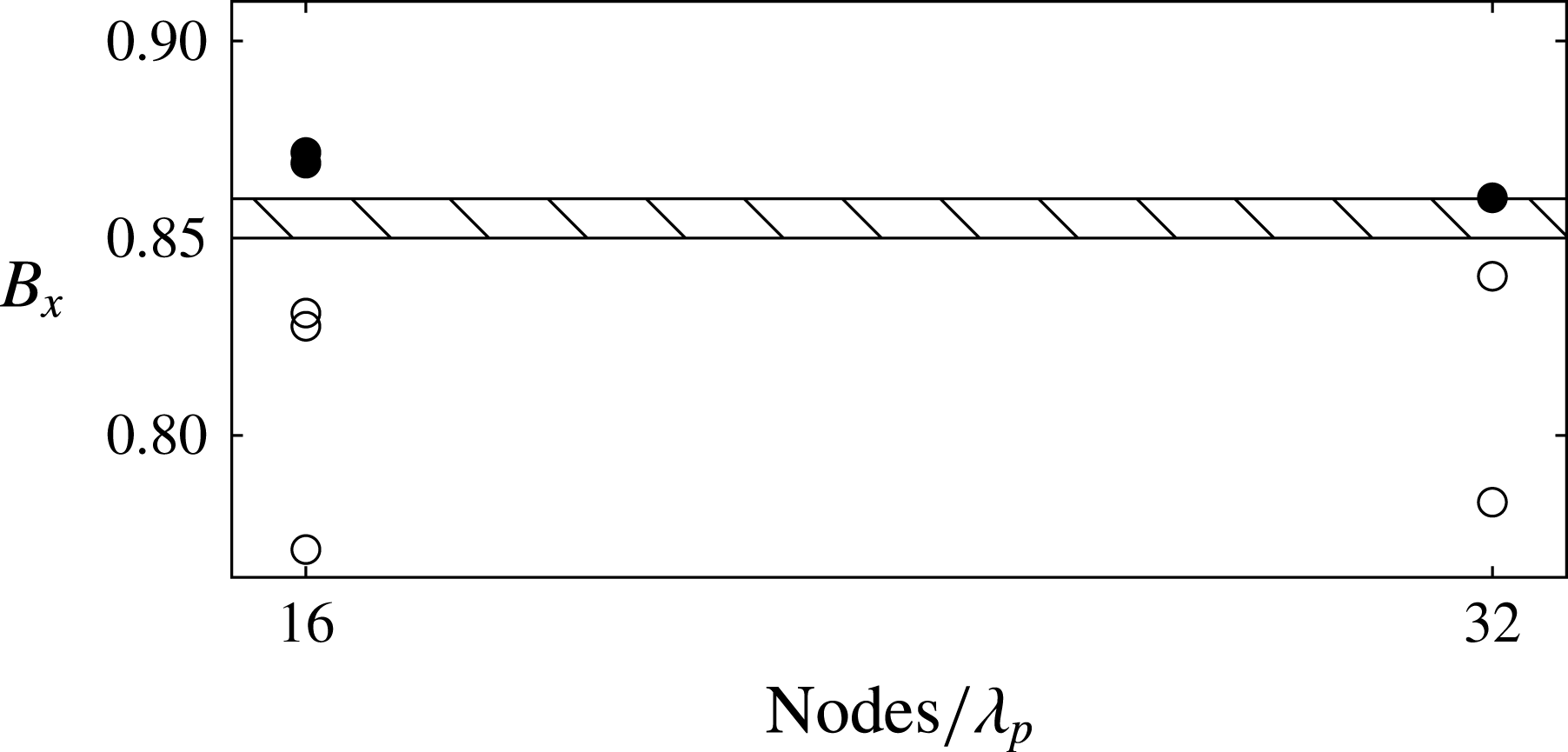
Breaking index
 $B_{x}$
versus average number of nodes per wavelength
 $\unicode[STIX]{x1D706}_{p}$
for the same C3N5 case. Filled circles indicate breaking crests, while open circles are recurrent crests. Each point is derived from the maximum of each individually tracked wave as in figures 4–6. The hatched breaking threshold zone based on our entire ensemble of derived
 $B_{x}$
values is seen to be relatively insensitive to the resolution.

The numerical experiments we ran for 2D C3N5 wave packets for different resolutions showed some minor differences. In this instance, the paddle amplitude necessary to reach maximum recurrence or marginal breaking reduced slightly between the R16 and R32 cases. The marginal breaking results for the slightly steeper R32 run produced slightly larger breaker amplitude, steepness and energy flux than the R16 case, consistent with the observed slightly shorter breaking onset epoch and corresponding fetch. However, for our primary goal of computing the derived breaking parameter
 $B_{x}$
, different resolutions for the same C3N5 wave group had only a minor influence on the determination of the threshold. Figure 10 confirms the convergence of the NWT simulations in determining the threshold zone for
 $B_{x}$
. Our proposed nominal breaking threshold value
 $B_{x}=0.85$
is well-bracketed for each resolution:
 $B_{x}$
is insensitive to the resolution and R16 is seen to be sufficient for our purpose of establishing a discriminating breaking criterion for 2D and 3D deep and intermediate depth water focusing wave packets.