





1. Introduction
When wind blows over an air–water interface, the resultant shear stress at the water surface induces a shear flow and its instability is one of main mechanisms for surface wave generation in the ocean (Miles Reference Miles1957; Sullivan & McWilliams Reference Sullivan and McWilliams2010). The vorticity in the shear flow is typically concentrated near the water surface and decays with depth.
In this paper, we study the simplest possible model of this situation, consisting of two layers of different vorticity in an inviscid fluid of constant density. The lower fluid layer of infinite depth is irrotational while the upper fluid layer has constant, uniform, vorticity. Mathematically, this leads to a nonlinear problem with two free boundaries: one is the internal interface at the vorticity jump, and the other is the free surface of constant pressure at the top of the shear layer.
The linear dispersion relation for a free-surface fluid with an internal vorticity jump was studied by Stern & Adam (Reference Stern and Adam1973) and Caponp et al. (Reference Caponp, Yuen, Milinazzo and Saffman1991), who both obtained a cubic equation for the wavespeed and observed that at certain parameter values this base state is unstable when two out of the three wavespeeds become identical. Weakly nonlinear corrections to the linear wavespeed were obtained by Brevik (Reference Brevik1978) by developing a Stokes expansion to third order, but the instability of the basic state and resonances between shear and gravity modes were not noticed. Fully nonlinear travelling-wave solutions were obtained numerically by Milinazzo & Saffman (Reference Milinazzo and Saffman1990) using a boundary-integral method. The nonlinear solutions obtained by Milinazzo & Saffman (Reference Milinazzo and Saffman1990) are characterised by a relatively large-amplitude surface displacement compared with that on the internal vorticity jump. However, out of the three possible solution branches that emerge from the cubic linear dispersion relation for the wavespeed, only the gravity-wave mode travelling in the direction of the shear flow was computed at finite amplitude in order to compare with the results of Banner & Phillips (Reference Banner and Phillips1974) for the dependence of the maximum wave amplitude on the surface drift. Nonlinear solutions corresponding to the remaining two solutions of the cubic linear dispersion relation were neglected entirely.
The aim of the present paper is to study the nonlinear solutions associated with the two remaining solutions of the cubic linear dispersion relation. These new solutions display behaviour previously unseen, namely relatively large-amplitude waves at the vorticity jump and bifurcations between solutions branches with different wavenumbers. Each bifurcation occurs across a very small region of parameter space, and results in significant changes in the solution profiles – including a reversal of the dominant-amplitude interface, and a change in the polarity (measuring the alignment of the two wave crests).
A time-dependent conformal mapping is developed to study the nonlinear travelling-wave solutions that emerge in our model formulation. Similar conformal mappings have been used by Dyachenko et al. (Reference Dyachenko, Zakharov and Kuznetsov1996) and Choi & Camassa (Reference Choi and Camassa1999) for a free-surface fluid of finite depth, Choi (Reference Choi2009) and Murashige & Choi (Reference Murashige and Choi2020) for a fluid layer of constant vorticity, Murashige & Choi (Reference Murashige and Choi2022) for the interface between two fluid layers and Blyth & Părău (Reference Blyth and Părău2016) for a fluid bounded both above and below by interfaces. The domain used in each of these approaches is analogous to both our irrotational fluid layer, bounded by a single interface, and to our shear layer of constant vorticity, bounded both above and below by interfaces. However, combining these two approaches to develop a conformal mapping appropriate to our model formulation raises an additional complication regarding continuity of solutions at the vorticity jump. This is resolved by creating an additional unknown at the internal interface to match each conformal domain together (see Murashige & Choi Reference Murashige and Choi2022, for an analogous approach). The principal advantage of the time-dependent conformal mapping over other steady boundary-integral approaches used by e.g. Milinazzo & Saffman (Reference Milinazzo and Saffman1990) is their time-dependent generalisation to study both stability and time evolution in general.
The paper is organised as follows. In § 2 we formulate the governing boundary-value problem for the nonlinear shear layer. The linear dispersion relation for the wavespeed is derived and some of the associated solutions are illustrated. The conformal mapping is developed in § 3; here, we provide the final boundary-integral formulation in § 3.4 and details of the numerical method in § 3.5. Nonlinear solutions and their properties are then described in § 4. A discussion of our results and our conclusions are offered in § 5.
2. Mathematical formulation
We now present the non-dimensional boundary-value problem for the evolution of of a layer of constant vorticity lying below a free surface and above an irrotational fluid layer of infinite depth. Throughout this work we refer to the upper interface as the free surface and refer to the lower interface as the vorticity interface. The free surface is located at
 $y=\zeta_1(x,t)$
, and the vorticity jump is located at
 $y=\zeta_2(x,t)$
. We consider a two-dimensional flow with
 $y$
pointing upwards and
 $x$
horizontally. We nondimensionalise with respect to the shear strength
 $\omega$
and constant of gravitational acceleration
 $g$
by taking
 $g/\omega ^2$
as a length scale and
 $1/\omega$
as a time scale. The irrotational fluid is located in the range
 $-\infty \lt y \leqslant \zeta _2(x,t)$
, and the rotational fluid (the shear layer) is located within
 $\zeta _2(x,t) \leqslant y \leqslant \zeta _1(x,t)$
. In denoting the (hereafter) non-dimensional velocity field in the upper layer by
 $\boldsymbol{u}_1=(u_1,v_1)$
and that in the lower layer by
 $\boldsymbol{u}_2=(u_2,v_2)$
, we decompose
 $\boldsymbol{u}_1=\boldsymbol{\nabla }\phi _1+(y,0)$
and
 $\boldsymbol{u}_2=\boldsymbol{\nabla }\phi _2$
, where
 $\phi _1(x,y,t)$
and
 $\phi _2(x,y,t)$
are the velocity potentials in each layer. The fluid domain and velocity field decomposition is depicted in figure 1.
The domain
 $-\infty \lt y \leqslant \zeta _1(x,t)$
of the irrotational fluid, and the domain
 $-\zeta _1(x,t) \leqslant y \leqslant \zeta _2(x,t)$
of the rotational fluid is depicted. The vorticity of the upper fluid layer is constant, and there we employ the Helmholtz decomposition of the velocity field into an irrotational (potential) part and a linear horizontal shear flow. The shear flow is of unit strength due to the non-dimensionalisation used. Periodicity in
 $x$
is assumed across the vertical dashed lines.

A derivation of the following boundary-value problem from the dimensional Euler equations is provided in Appendix A. First, the velocity potential in each layer satisfies Laplace’s equation
 \begin{align} {\nabla} ^2 \phi _1 &=0 \quad \text{for } \quad \zeta _{2}(x,t) \leqslant y \leqslant \zeta _1(x,t), \\[-12pt]\nonumber \end{align}
 \begin{align} {\nabla} ^2 \phi _2 &=0 \quad \text{for} \quad -\infty \lt y \leqslant \zeta _2(x,t). \end{align}
At the free surface,
 $y=\zeta _1(x,t)$
, there are both kinematic and dynamic boundary conditions given by
 \begin{align} \zeta _{1t}=\phi _{1y}-\zeta _{1x}(\phi _{1x}+ y) \quad &\text{at } \quad y=\zeta _1(x,t), \\[-12pt]\nonumber \end{align}
 \begin{align} \phi _{1t} +\frac {1}{2}(\phi _{1x}^2+\phi _{1y}^2)+ y(\phi _{1x}+1)- \psi _1 =B_1 \quad &\text{at } \quad y=\zeta _1(x,t), \end{align}
respectively. The function
 $\psi _1(x,y,t)$
is the harmonic conjugate of
 $\phi _1(x,y,t)$
, and
 $B_1$
is the Bernoulli constant. The boundary conditions holding at the vorticity interface
 $y=\zeta _2(x,t)$
are the kinematic condition and continuity of velocity, given by
 \begin{align} \zeta _{2t}=\phi _{2y}-\zeta _{2x}\phi _{2x} \quad &\text{at } \quad y=\zeta _2(x,t), \\[-12pt]\nonumber \end{align}
 \begin{align} \phi _{1x}+y = \phi _{2x}, \quad \phi _{1y}=\phi _{2y} \quad &\text{at } \quad y=\zeta _2(x,t). \end{align}
Note that the shear flow in the upper fluid layer gives rise to all terms involving
 $y$
in (2.1c
) and (2.1f
), as well as the terms
 $y \phi _{1x}$
and
 $\psi _1$
in (2.1d
).
Lastly, we have far-field decay conditions on the velocity potential
 $\phi _2$
and its harmonic conjugate
 $\psi _2$
given by
 \begin{equation} (\phi _2,\psi _2) \to (0,0) \quad \text{as } \quad y \to -\infty . \end{equation}
To summarise, the boundary-value problem (2.1) involves the unknown solutions
 $\zeta _1$
,
 $\zeta _2$
,
 $\phi _1$
and
 $\phi _2$
, together with the Bernoulli constant
 $B_1$
. By fixing the total volume of fluid in each layer, we obtain from Appendix A.2.1 the constraints
 \begin{equation} \frac {1}{L}\int _{-L/2}^{L/2} \zeta _1 \, \mathrm{d}x =H \quad \text{and} \quad \int _{-L/2}^{L/2} \zeta _2 \,\mathrm{d}x=0, \end{equation}
where the (non-dimensional) parameters
 $L$
and
 $H$
are given by
 \begin{equation} L= \frac {\lambda \omega ^2}{g} \quad \text{and} \quad H=\frac {h \omega ^2}{g}. \end{equation}
Here,
 $\lambda$
is the wavelength,
 $\omega$
is the shear strength,
 $g$
is the constant acceleration of gravity and
 $h$
is the mean depth of the shear layer. Thus,
 $L$
is the non-dimensional wavelength and
 $H$
is the non-dimensional mean shear-layer depth. Note that the limit of
 $g \to 0$
in which gravity is absent results in
 $L \to \infty$
and
 $H \to \infty$
. Further, there are two distinguished limits in which the shear layer is removed: as
 $h \to 0$
we have
 $H \to 0$
, and as
 $\omega \to 0$
we have both
 $L \to 0$
and
 $H \to 0$
.
When solving for small-amplitude solutions in § 2.1, the resultant (possibly complex-valued) wavespeed
 $c$
is a function of
 $L$
and
 $H$
. When solving for nonlinear travelling waves of permanent form, the real-valued
 $c$
in this case depends additionally on a measure of the amplitude of the solution, detailed below. In both cases,
 $c$
is the unknown of the problem.
2.1. The linear dispersion relation
We now study the behaviour and dispersion relation of small-amplitude solutions. When the amplitudes of both the free surface and vorticity interface are zero, an exact solution is known to the boundary-value problem (2.1), given by
 $\zeta _1=H$
,
 $\zeta _2=0$
and
 $\phi _1=\phi _2=\psi _1=\psi _2=0$
. Thus, in the study of small-amplitude solutions we consider
 \begin{equation} \zeta _1 \sim H+\epsilon \bar {\zeta }_1, \quad \zeta _2 \sim \epsilon \bar {\zeta }_2 , \quad \phi _1 \sim \epsilon \bar {\phi }_1, \quad \phi _2 \sim \epsilon \bar {\phi }_2, \quad \psi _1 \sim \epsilon \bar {\psi }_1, \quad \psi _2 \sim \epsilon \bar {\psi }_2, \end{equation}
which hold as
 $\epsilon \to 0$
. Further, the Bernoulli constant is expanded as
 $B_1 \sim H+ \epsilon \bar {B}_1$
. In order to solve for the perturbation quantities in (2.4) above, we first have to obtain the governing equations at
 $O(\epsilon )$
. Note that the boundary conditions are evaluated at
 $y=\zeta _1(x,t)$
and
 $y=\zeta _2(x,t)$
, which are also expanded in
 $\epsilon$
; these conditions are resolved by Taylor expanding each term.
The equations obtained at
 $O(\epsilon )$
are
 ${\nabla} ^2 \bar {\phi _1}=0$
for
 $0 \leqslant y \leqslant H$
, and
 ${\nabla} ^2 \bar {\phi }_2=0$
for
 $-\infty \lt y \leqslant 0$
. The far-field conditions are
 $(\bar {\phi }_2,\bar {\psi }_2) \to (0,0)$
as
 $y \to - \infty$
. The boundary conditions holding at
 $y=0$
are
 $\bar {\zeta }_{2t}=\bar {\phi }_{2y}$
,
 $\bar {\phi }_{2y}=\bar {\phi }_{1y}$
,
 $\bar {\phi }_{2x}=\bar {\phi }_{1x}+ \bar {\zeta }_2$
and
 $\bar {\psi }_2=\bar {\psi }_1$
. Those holding at
 $y=H$
are
 $\bar {\zeta }_{1t}=\bar {\phi }_{1y}-H\bar {\zeta }_{1x}$
and
 $\bar {\phi }_{1t}+H\bar {\phi }_{1x}-\bar {\psi }_1+\bar {\zeta }_1=\bar {B}_1$
. The solutions to these can be written as
 \begin{align} \{ \bar {\zeta }_1 , \bar {\zeta }_2 \} &= \{ \alpha , \beta \}\mathrm{e}^{ {i}k(x - ct)}+\text{c.c.}, \\[-12pt]\nonumber \end{align}
 \begin{align} \{ \bar {\phi }_1 , \bar {\psi }_1 \} &= \big [ \{ \mu , \mathrm{i}\mu \}\mathrm{e}^{k y}+\{ \nu , -\mathrm{i}\nu \}\mathrm{e}^{-k y}\big ]\mathrm{e}^{{i}k(x - ct)} +\text{c.c.}, \\[-12pt]\nonumber \end{align}
 \begin{align} \{ \bar {\phi }_2 , \bar {\psi }_2 \} &=\{ \gamma , \mathrm{i}\gamma \}\mathrm{e}^{ {i}k(x - ct)}\mathrm{e}^{k y}+\text{c.c.}, \end{align}
where
 $\text{c.c.}$
denotes complex conjugate and
 $k=2 \pi n /L$
is the wavenumber (
 $n$
is a positive integer). The solutions in (2.5b
) and (2.5c
) satisfy Laplace’s equation, the Cauchy–Riemann equations applied to the analytic functions
 $\bar {\phi }_1+\mathrm{i}\bar {\psi }_1$
and
 $\bar {\phi }_2+\mathrm{i}\bar {\psi }_2$
, as well as the decay conditions
 $(\bar {\phi }_2,\bar {\psi }_2) \to (0,0)$
. In (2.5),
 $c \in \mathbb{C}$
is the complex-valued unknown whose real and imaginary parts are the speed and growth rate of the perturbations, respectively.
Substituting solutions (2.5) into the
 $O(\epsilon )$
equations yields the algebraic equations
 \begin{align} &\gamma =\mu -\nu , \qquad \mathrm{i}k\gamma =\beta + \mathrm{i}k(\mu +\nu ), \qquad \gamma =-\mathrm{i}c\beta ,\nonumber \\ &\mathrm{i}(H-c)\alpha =\mu \mathrm{e}^{k H}-\nu \mathrm{e}^{-k H} \qquad \textrm {and}\nonumber \\ &\mathrm{i}k(H-c)[\mu \mathrm{e}^{kH} + \nu \mathrm{e}^{-kH}]-\mathrm{i}[\mu \mathrm{e}^{kH} - \nu \mathrm{e}^{-kH}]+\alpha =0. \end{align}
In solving this set of five equations for the five unknown constants, non-trivial solutions exist only when the dispersion relation
 \begin{equation} (H-c+1)\big (2 kc-1+\mathrm{e}^{-2kH}\big ) =k(H-c)^2 \big (2k c-1-\mathrm{e}^{-2kH}\big ) \end{equation}
is satisfied. This is a cubic equation for the unknown
 $c$
, in terms of
 $H$
and
 $k=2 \pi n/L$
. The real part,
 $\text{Re}[c]$
, corresponds to the wavespeed of time-dependent perturbations to the flat wave state, and the imaginary part,
 $\text{Im}[c]$
, to the growth rate of the perturbations.
Solutions to the cubic linear dispersion relation (2.7) are shown for
 $H=1$
in
 $(a)$
, and for
 $L=5$
in
 $(b)$
. Values of Re
 $[c]$
are shown in black and values for Im
 $[c]$
in grey. In each figure there is a range of parameters for which unstable perturbations exist with Im
 $[c]\gt 0$
, and the real parts of the wavespeed in these cases are shown with dotted lines. This occurs when two solutions of the cubic have the same real part and are complex conjugates of one another. The points of marginal stability are indicated with circles, and these are studied further across the parameter space in figure 3.

Solutions of the cubic dispersion relation (2.7) are shown in figure 2 for
 $n=1$
, firstly for
 $H=1$
in figure 2
 $(a)$
and for
 $L=5$
in figure 2
 $(b)$
. In each case, we see that there is a range of the remaining parameter (
 $L$
or
 $H$
) for which the time-dependent perturbation is unstable. For instance, in figure 2
 $(a)$
, which has
 $H=1$
, there are three marginally stable modes (solutions with Im
 $[c]=0$
) for
 $0\leqslant L \leqslant 2.1589$
and
 $L \geqslant 2.5814$
. When
 $2.1589\lt L\lt 2.5814$
, there is one marginally stable mode and two complex-conjugate modes with
 $\text{Im}[c] \neq 0$
; these correspond to stable and unstable modes with the same value of the wavespeed,
 $\text{Re}[c]$
.
Values of
 $H$
and
 $L$
for which small-amplitude perturbations to the base state,
 $\zeta _1(x,t)=H$
and
 $\zeta _2(x,t)=0$
, are marginally stable are shown. This corresponds to two repeated real-valued roots to the cubic dispersion relation (2.7) for
 $c$
. We have taken
 $n=1$
which results in one wave period within the periodic domain. Black curves show the edge of the marginally stable parameter region, within which the linear solutions are unstable. Black circles correspond to the four locations of marginal stability seen in figure 2. This figure is comparable to figure 1 from Caponp et al. (Reference Caponp, Yuen, Milinazzo and Saffman1991).

The values of
 $H$
and
 $L$
that correspond to the edge of the region of instability may be determined by further studying the cubic dispersion relation (2.7). At the edge of the instability region, the complex-conjugate roots have
 $\text{Im}[c]=0$
and therefore are repeated roots. In writing this dispersion relation in the form
 $c^3 + a_2 c^2 + a_1 c +a_0=0$
, where
 $a_0$
,
 $a_1$
and
 $a_2$
are known functions of
 $L$
and
 $H$
, we identify a repeated root by factorising the cubic as
 $(c-\alpha )^2(c-\beta )=0$
, where
 $c=\alpha$
is the repeated root. Equating these two representations of the cubic dispersion relation yields three constraints for the two unknowns
 $\alpha$
and
 $\beta$
. Two of these constraints determine
 $\alpha =-a (a_2 + \sqrt {a_2^2-3a_1} )/3$
and
 $\beta =-a_2-2\alpha$
, and the remaining constraint requires
 $\alpha ^2 (a_2 + 2\alpha )-a_0=0$
, which forms an implicit relation for
 $L$
and
 $H$
. We solve this constraint numerically by Newton iteration, the results of which are shown in figure 3 with
 $n=1$
. Two branches of parameter values exist as shown in this figure. For every value of
 $H$
, there exists a range of values of
 $L$
for which the time-dependent perturbation of the base state is unstable.
We can also study the three solutions of dispersion relation (2.7) under the limits of
 $k \to 0$
and
 $k \to \infty$
. Firstly, for the long-wave limit of
 $k \to 0$
we obtain
 \begin{equation} c \sim H -H^2 k \quad \textrm {and}\quad c \sim \pm k^{-1/2} + \frac {H^2}{2}k, \end{equation}
and for short waves with
 $k \to \infty$
we obtain
 \begin{equation} c \sim \frac {1}{2}k^{-1} \quad \textrm {and}\quad c \sim H \pm k^{-1/2}. \end{equation}
In each case, the two latter modes correspond to gravity waves on infinite depth in the presence of a mean current.
2.2. Travelling-wave solutions of small amplitude
When the wavespeed
 $c$
is real valued, the small-amplitude disturbances studied in § 2.1 are travelling waves. The corresponding solutions for each interface are then given by
 \begin{align} \zeta _1(x,t) &\sim H + A \cos {\big (k (x-ct)\big )}, \\[-12pt]\nonumber \end{align}
 \begin{align} \zeta _2(x,t) &\sim -\frac {2k(H-c)\mathrm{e}^{-kH}}{(2kc-1)+\mathrm{e}^{-2kH}} A\cos {\big ( k (x-ct)\big )}, \end{align}
where
 $0 \leqslant A \ll 1$
, and
 $k=2 \pi n/L$
. We have considered the case for which
 $A$
is non-negative without any loss of generality – the case with negative
 $A$
is captured automatically due to translational invariance. Recall that
 $\zeta _1(x,t)$
is the free surface that bounds the rotational fluid with a region of uniform pressure, and
 $\zeta _2(x,t)$
is the vorticity interface between the two fluids. Two interesting cases emerge in the linear solutions (2.9). Firstly, if
 $c =c_1=(1- \mathrm{e}^{-2kH})/(2k)$
, then the solution for
 $\zeta _1(x,t)$
in (2.9a
) is constant,
 $\zeta _1=H$
. This corresponds to a travelling wave on the vorticity interface when the top free surface is replaced by a rigid boundary, which was studied by Rayleigh (Reference Rayleigh1894). Therefore,
 $c=c_1$
represents the linear speed of the shear wave mode. Secondly, if
 $c=c_2=H$
, then the solution for
 $\zeta _2(x,t)$
in (2.9b
) is identically zero. This corresponds to a linear surface wave and a zero-amplitude vorticity interface.
Branches of travelling-wave solutions are shown with solid lines in the
 $(H,c)$
plane for fixed
 $L=5$
,
 $n=1$
and
 $A=10^{-5}$
from the amplitude condition (2.10). The condition
 $c_1=(1-\mathrm{e}^{-2kH})/(2k)$
which results in
 $\zeta _1(x)=0$
is shown dotted, and
 $c_2=H$
which results in
 $\zeta _2(x)=0$
is shown dashed. Panels
 $(a)$
to
 $(i)$
show the nine labelled solution profiles. In these, the free surface
 $\zeta _1(x)$
is shown in black, and the vorticity interface
 $\zeta _2(x)$
is shown dashed. Note that we have plotted
 $\zeta _1-H$
in order to see the surface profile more clearly. The upper branch with the largest value of
 $c$
corresponds to the solutions calculated by Milinazzo & Saffman (Reference Milinazzo and Saffman1990).

Figure 4. Long description
The image contains a combination of line graphs and solution profiles. Panel A shows a line graph with the horizontal axis labeled H and the vertical axis labeled c. The graph includes solid, dotted, and dashed lines representing different conditions for the wavespeed. Key points labeled a through i mark specific solution profiles. Panels B to I display the nine labeled solution profiles, each showing the free surface in black and the vorticity interface in dashed lines. The horizontal axis in these panels is labeled x over L, and the vertical axis is labeled y over L. Each profile illustrates the surface and vorticity interface displacements for different parameter values. The upper branch with the largest value of c corresponds to the solutions calculated by Milinazzo & Saffman (1990).
Notice that the solutions with
 $c_1=(1- \mathrm{e}^{-2kH})/(2k)$
and
 $c_2 =H$
are obtained as possible solutions from the linear dispersion (2.7) relation only in the limits of
 $H \to \infty$
and
 $H \to 0$
with
 $k \to \infty$
such that
 $kH$
is finite. These values of
 $c$
are shown in the
 $(c,H)$
plane in figure 4 for
 $n=1$
and
 $L=5$
, where the solid lines are solutions of the dispersion relation with
 $\text{Im}[c]=0$
. Here, the values of
 $c_1$
are indicated by the dotted line and those of
 $c_2$
by the dashed line. By expanding the dispersion relation as
 $H \to \infty$
, the two solution branches parallel to
 $c_2=H$
as
 $H \to \infty$
in figure 4 may be obtained as
 $c \sim H -1/(2k) \pm \sqrt {(1+4k)/(4k^2)} +O(H^{-1})$
, and therefore represent two gravity modes on an infinite-depth fluid with constant vorticity.
As a measure of the solution amplitude, we employ the sum of individual amplitudes defined by
 \begin{equation} A=\frac {\text{max}(\zeta _1)-\text{min}(\zeta _1) + \text{max}(\zeta _2)-\text{min}(\zeta _2)}{L}, \end{equation}
which is positive definite and tends to zero in the small-amplitude limit of
 $\epsilon \to 0$
from (2.4). Note that there are many ways to define an amplitude condition for these solutions. For instance, in the study by Milinazzo & Saffman (Reference Milinazzo and Saffman1990), the condition
 $\text{max}(\zeta _1)-\text{min}(\zeta _1)$
was used, but this has the issue of permitting highly nonlinear vorticity interfaces with
 $\zeta _2 =O(1)$
in the limit of small amplitude. Alternative choices are the momentum and energy derived in Appendix A.2, which are conserved quantities of the time-dependent system. However, the value of these is finite and non-zero in the small-amplitude limit; moreover when shifted by a constant to ensure that the momentum and energy tend to zero in the small-amplitude limit, they fail to be positive definite.
Branches of linear solutions are shown in the
 $(H,c)$
plane for
 $L=5$
and
 $A=10^{-5}$
. The three branches with
 $n=1$
were shown in figure 4. Here,
 $n$
represents the number of wave periods within the periodic domain. Also shown are the solution branches with
 $n=2$
(dashed) and
 $n=3$
(dotted). Solution branches with different wavenumbers intersect with one another, which leads to the bifurcations of nonlinear solutions studied in § 4.

Small-amplitude solutions are shown across each of the three solution branches in figure 4 for
 $L=5$
. These solutions were calculated with an amplitude of
 $A=10^{-5}$
from (2.10). Along the solution branch with the largest value of the wavespeed
 $c$
corresponding to the gravity-wave mode travelling in the same direction as the shear flow, the amplitude of the free surface
 $\zeta _1(x)$
is large and the amplitude of the vorticity interface
 $\zeta _2(x)$
is small. This is seen in profiles figure 4(a–c) here, as
 $H \to \infty$
along this branch we have
 $\zeta _2 \to 0$
. The remaining two solution branches consist of solutions with a larger-amplitude vorticity interface. The branch starting from
 $c=0$
corresponds to the shear wave mode while the remaining branch represents the gravity-wave mode travelling in the opposite direction to the shear flow. These two modes collide as the value of
 $H$
increases and subsequently lose their stability. Along the solution branch containing
 $d$
,
 $e$
and
 $f$
, or before the collision occurs, the free surface and vorticity interface have the same polarity, whereas along branch
 $g$
,
 $h$
,
 $i$
this polarity is opposite to one another. Along these two branches, we have that the
 $\zeta _1(x) \to 0$
as
 $H \to 0$
starting from solution
 $d$
, and also as
 $H \to \infty$
starting from solution
 $i$
. Further, on the third solution branch we have
 $\zeta _2(x) \to 0$
as
 $H \to \infty$
when starting from solution
 $g$
.
All solutions shown in figure 4 have
 $n=1$
(which enters into the wavenumber
 $k=2 \pi n/L$
), and so have one wave period within the periodic domain. The linear dispersion relation (2.7) involves
 $k$
, and so branches computed with different wavenumbers have different values of the wavespeed
 $c$
. The linear branches of solutions with
 $n=1$
,
 $n=2$
and
 $n=3$
are shown in figure 5 for
 $L=5$
. We see that solution branches with different wavenumbers intersect with one another at multiple places. This means that at certain parameter values, there exist linear modes with different wavenumbers that travel at the same speed. In general, if it exists, this so-called resonance between gravity and shear wave modes with wavenumbers
 $k_n=2\pi n/L$
and
 $k_m=2\pi m/L$
can occur at two wavespeeds determined from (2.7) by
 \begin{equation} \frac {\big (2 k_nc-1+\mathrm{e}^{-2k_nH}\big )}{n \big (2k_n c-1-\mathrm{e}^{-2k_nH}\big )}= \frac {\big (2 k_mc-1+\mathrm{e}^{-2k_mH}\big )}{m \big (2k_m c-1-\mathrm{e}^{-2k_mH}\big )}\,. \end{equation}
Analogous behaviour arises for gravity-capillary waves on infinite depth as first shown by Wilton (Reference Wilton1915). A weakly-nonlinear theory was developed by Chen & Saffman (Reference Chen and Saffman1979) to resolve this issue for gravity-capillary waves, and it was shown that when linear dispersion curves cross there emerge bifurcations between these, which was later confirmed in a numerical work by Chen & Saffman (Reference Chen and Saffman1980). The same phenomenon emerges in our model formulation due to the crossing of linear solution branches. A numerical method to study this phenomenon for fully nonlinear solutions is now developed.
3. The boundary-integral formulation
In order to obtain numerical solutions to the nonlinear boundary-value problem (2.1), we employ a conformal map which takes the free surface
 $y=\zeta _1(x,t)$
and vorticity jump
 $y=\zeta _2(x,t)$
to a known location in the conformal domain. We first develop the time-dependent conformal mapping in § 3.1 to § 3.3, and then reduce this to the steady conformal mapping in § 3.4. The remainder of the paper focuses on computing travelling-wave solutions in a co-moving frame of speed
 $c$
with the steady conformal mapping; however, the method is first developed for the fully time-dependent case so that time evolution and stability can be studied in subsequent works without changing the formulation.
3.1. The time-dependent conformal mapping
The time-dependent mapping from the physical
 $(x,y)$
plane to the conformal
 $(\xi ,\eta )$
plane is shown. Each fluid region,
 $-\infty \lt y \leqslant \zeta _2$
and
 $\zeta _2 \leqslant y \leqslant \zeta _1$
, involves a distinct conformal map. The function
 $\gamma (\xi ,t)$
is introduced in § 3.2 to enforce continuity of physical quantities across each mapped region at
 $\eta =0$
.

Figure 6. Long description
A diagram illustrating the time-dependent mapping from the physical plane to the conformal plane for two fluid regions. Panel A: The left side of the diagram shows the physical plane with two distinct fluid regions, labeled as y = ξ1(x, t) and y = ξ2(x, t). The regions are depicted with curved lines representing the fluid surfaces at different times. The x and y axes are labeled, indicating the spatial dimensions. Panel B: The right side of the diagram shows the conformal plane with a grid representing the mapped regions. The η and ξ axes are labeled, indicating the conformal dimensions. The top boundary is labeled as η = h(t), and the bottom boundary is labeled as η = 0. Arrows indicate the mapping functions x(ξ1, η1, t), y(ξ1, η1, t), x(ξ2, η2, t), and y(ξ2, η2, t), showing the transformation from the physical plane to the conformal plane for each fluid region.
A different conformal map must be used for each of the two fluid layers. For the irrotational fluid confined within
 $-\infty \lt y \leqslant \zeta _2(x,t)$
, we consider the map that takes
 $(x,y)$
to
 $(\xi _2,\eta _2)$
, such that the fluid is located in the range
 $-\infty \lt \eta _2 \leqslant 0$
. For the rotational fluid located in the range
 $\zeta _2(x,t) \leqslant y \leqslant \zeta _1(x,t)$
, we consider the map that takes
 $(x,y)$
to
 $(\xi _1,\eta _1)$
, such that the fluid is located in the range
 $0 \leqslant \eta _1 \leqslant h(t)$
. This mapping is depicted in figure 6. The conformal method developed in this section was originally derived for a single bounded fluid layer (Choi & Camassa Reference Choi and Camassa1999) and was extended to the case of two unbounded fluid layers by Murashige & Choi (Reference Murashige and Choi2022). Our implementation requires the combination of an unbounded lower layer for the irrotational fluid, and a bounded upper region for the vorticity layer.
The solutions in the lower fluid layer are then given by
 $x_2(\xi _2,\eta _2,t)$
,
 $y_2(\xi _2,\eta _2,t)$
,
 $\phi _2(x_2(\xi _2,\eta _2,t),y_2(\xi _2,\eta _2,t),t)$
and
 $\psi _2(x_2(\xi _2,\eta _2,t),y_2(\xi _2,\eta _2,t),t)$
. Each of these satisfies Laplace’s equation within the conformal domain (i.e.
 ${\nabla} ^2 y_2 = \partial ^2_{\xi _2} y_2 + \partial ^2_{\eta _2} y_2=0$
). Further, we have the decay conditions
 $x_2\sim \xi _2$
,
 $y_2 \sim \eta _2$
,
 $\phi _2 \to 0$
and
 $\psi _2 \to 0$
as
 $\eta _2 \to -\infty$
, the first two of which are obtained from requirements of the map, and the latter two from (2.1g
). Since the functions
 $x_2+\mathrm{i}y_2$
and
 $\phi _2 + \mathrm{i}\psi _2$
are harmonic, it suffices to solve only for the imaginary part of each and then use the Cauchy–Riemann equations to obtain the solution for the real part. The solutions of these conformal boundary-value problems are then given by
 \begin{align} \{ x_2,y_2 \} &=\{\xi _2 , \eta _2\}+\sum _{\substack {m=-\infty \\ m \neq 0}}^{\infty } \big \{ \! - \mathrm{i}\boldsymbol{\cdot }\text{sgn}(m)a_m(t), a_m(t)\big \}\mathrm{e}^{ |m|k \eta _2}\mathrm{e}^{{i} m k \xi _2}, \\[-12pt]\nonumber \end{align}
 \begin{align} \{ \phi _2,\psi _2 \} &=\sum _{\substack {m=-\infty \\ m \neq 0}}^{\infty } \big \{ \! - \mathrm{i}\boldsymbol{\cdot }\text{sgn}(m)b_m(t),b_m(t)\big \}\mathrm{e}^{|m|k \eta _2}\mathrm{e}^{{i} m k \xi _2}, \end{align}
where
 $\text{sgn}(m)$
is the signum function and
 $k=2 \pi n/L$
.
In the upper fluid layer, we denote the solutions by
 $x_1(\xi _1,\eta _1,t)$
,
 $y_1(\xi _1,\eta _1,t)$
,
 $\phi _1(x_1(\xi _1,\eta _1,t),y_1(\xi _1,\eta _1,t),t)$
and
 $\psi _1(x_1(\xi _1,\eta _1,t),y_1(\xi _1,\eta _1,t),t)$
. These satisfy Laplace’s equation for
 $0 \leqslant \eta _1 \leqslant h(t)$
, as well as matching constraints with the solutions (3.1) of the lower fluid layer at
 $\eta _1=0$
. A difficulty that arises with this matching is that the horizontal conformal coordinates are not equal at the vorticity interface
 $\eta _2=0$
and
 $\eta _1=0$
, and require the introduction of an intermediary variable (which itself is an unknown of the problem). This process is detailed further in § 3.2. The solutions in the upper fluid layer may be obtained as
 \begin{align} y_1 &=\eta _1+c_0(t) +\sum _{\substack {m=-\infty \\ m \neq 0}}^{\infty } \big [c_m(t)\mathrm{e}^{m k \eta _1}+d_m(t)\mathrm{e}^{-mk \eta _1}\big ]\mathrm{e}^{{i} m k \xi _1}, \\[-12pt]\nonumber \end{align}
 \begin{align} \phi _1 &= e_0(t) \xi _1 +f_0(t) \eta _1+g_0(t)+\sum _{\substack {m=-\infty \\ m \neq 0}}^{\infty }\big [e_m(t)\mathrm{e}^{m k \eta _1}+f_m(t)\mathrm{e}^{-m k \eta _1}\big ]\mathrm{e}^{{i} m k \xi _1}. \end{align}
Solutions for
 $x_1$
and
 $\psi _1$
can be obtained by integrating the Cauchy–Riemann equations
 $x_{1\xi _1}=y_{1\eta _1}$
and
 $\psi _{1 \xi _1}=-\phi _{1 \eta _1}$
, with the constant of integration for
 $x_1$
determined by the condition
 $x_1(0,0,t)=0$
.
In this formulation, we restrict solutions (3.1) in the lower fluid layer to
 $\eta _2=0$
, and (3.2) solutions in the upper fluid layer to both
 $\eta _1=0$
and
 $\eta _1=h(t)$
. The solutions on the boundaries are represented with capital letters, for instance those for the vertical coordinates
 $y_1$
and
 $y_2$
are
 \begin{align} Y_{1U}(\xi _1,t)=y_1(\xi _1,h(t),t), \quad Y_{1L}(\xi _1,t)=y_1(\xi _1,0,t), \quad Y_{2U}(\xi _2,t)=y_2(\xi _2,0,t). \end{align}
The subscript number refers to the original fluid layer, while the subscript letter denotes whether the solution has been evaluated at the upper or lower surface that bounds the respective layer. For instance,
 $Y_{1U}$
denotes the solution
 $y_1(\xi _1,\eta _1,t)$
evaluated at the upper interface
 $\eta _1=h(t)$
of layer one. Equivalent definitions are also introduced for
 $X_{1U}$
,
 $X_{1L}$
,
 $X_{2U}$
,
 $\varPhi _{1U}$
,
 $\varPhi _{1L}$
,
 $\varPhi _{2U}$
,
 $\varPsi _{1U}$
,
 $\varPsi _{1L}$
and
 $\varPsi _{2U}$
.
The quantities for the lower fluid layer are related by the Hilbert transform (see below), giving
 \begin{equation} X_{2U}=\xi _2 - \mathscr{H}\,\,[Y_{2U}], \quad \varPhi _{2U}=-\mathscr{H}\,\,[\varPsi _{2U}]. \end{equation}
The harmonic relations (3.4) relate the real and imaginary parts of an analytic function that decays to zero as
 $\eta _2 \to -\infty$
. Note that the relation
 $\varPsi _{2U}=\mathscr{H}\,\,[\varPhi _{2U}]$
is also required for the time-dependent mapping, in which an evolution equation is first obtained for
 $\varPhi _{2U}$
. The operator
 $\mathscr{H}\,$
appearing in (3.4) is the Hilbert transform, defined by
 \begin{equation} \mathscr{H}\,\,[Y] =\frac {1}{\pi }\,{\int \!\!\!\!\!\!{-}}_{-\infty }^{\infty }\frac {Y(\tilde {\xi })}{\tilde {\xi }-\xi } \mathrm{d}{\tilde {\xi }}. \end{equation}
Analogous harmonic relations are obtained for the quantities for the upper fluid layer, which are given by
 \begin{equation} X_{1L}=\xi _1 + \mathscr{T}\,\,[Y_{1L}] -\mathscr{S}\,\,[Y_{1U}], \quad X_{1U}=\xi _1+\mathscr{S}\,\,[Y_{1L}]-\mathscr{T}\,\,[Y_{1U}], \end{equation}
 \begin{equation} \varPhi _{1L}^{\prime }=A_0 + \mathscr{T}\,\,[\varPsi _{1L}^{\prime }] -\mathscr{S}\,\,[\varPsi _{1U}^{\prime }], \quad \varPhi _{1U}^{\prime }=A_0+\mathscr{S}\,\,[\varPsi _{1L}^{\prime }]-\mathscr{T}\,\,[\varPsi _{1U}^{\prime }], \end{equation}
where
 $A_0=(L h)^{-1}\int _{-L/2}^{L/2} [\varPsi _{1U}-\varPsi _{1L}] \mathrm{d}\xi _2$
. The operators
 $\mathscr{T}$
and
 $\mathscr{S}$
are principal-valued integrals defined by
 \begin{equation} \mathscr{T}\,\,[Y]={\int \!\!\!\!\!\!{-}}_{-\infty }^{\infty }\frac {Y(\tilde {\xi })}{2h} \coth {\bigg [\frac {\pi (\tilde {\xi }-\xi )}{2h}\bigg ]} \mathrm{d}{\tilde {\xi }}, \quad \mathscr{S}\,\,[Y]={\int \!\!\!\!\!\!{-}}_{-\infty }^{\infty }\frac {Y(\tilde {\xi })}{2h} \tanh {\bigg [ \frac {\pi (\tilde {\xi }-\xi )}{2h}\bigg ]} \mathrm{d}{\tilde {\xi }}, \end{equation}
where
 $h=L^{-1}\int _{-L/2}^{L/2}(Y_{1U}-Y_{1L})\mathrm{d}\xi _1$
. In practise, we calculate each of the three principal-valued integrals spectrally with the Fourier multipliers detailed in § 3.5.
By using the chain rule, expressions can be obtained for partial derivatives with respect to
 $x$
and
 $y$
in terms of the conformal coordinates
 $\xi _1$
and
 $\eta _1$
, or
 $\xi _2$
and
 $\eta _2$
. The Cauchy–Riemann equations are then used to eliminate derivatives with respect to
 $\eta _1$
and
 $\eta _2$
. This results in expressions which only involve differentiation with respect to
 $\xi _1$
or
 $\xi _2$
, which are used to convert the two-dimensional boundary-value problem (2.1) into a one-dimensional boundary-integral formulation. We use primes
 $(\prime )$
to denote differentiation with respect to either
 $\xi _1$
or
 $\xi _2$
, depending on the dependence of the function. For instance,
 $Y_{1U}^{\prime }$
denotes
 $\partial _{\xi _1}Y_{1U}$
. We then obtain
 $\zeta _{1x}=Y_{1U}^{\prime }/X_{1U}^{\prime }$
,
 $\zeta _{2x}=Y_{1L}^{\prime }/X_{1L}^{\prime }$
and
 $\zeta _{2x}=Y_{2U}^{\prime }/X_{2U}^{\prime }$
for the derivatives of each interface. Derivatives of the velocity potential are found to be
 $\phi _{1x}=(Y_{1U}^{\prime } \varPsi _{1U}^{\prime } + X_{1U}^{\prime } \varPhi _{1U}^{\prime })/J_{1U}$
and
 $\phi _{1y}=(Y_{1U}^{\prime } \varPhi _{1U}^{\prime }- X_{1U}^{\prime } \varPsi _{1U}^{\prime })/J_{1U}$
, with equivalent results holding for
 $\phi _{1x}$
,
 $\phi _{1y}$
,
 $\phi _{2x}$
and
 $\phi _{2y}$
evaluated at the lower interface,
 $\eta _1=\eta _2=0$
. Here, we have defined
 $J_{1U}(\xi _1,t)=(X_{1U}^{\prime })^2+(Y_{1U}^{\prime })^2$
and
 $J_{2L}(\xi _2,t)=(X_{2L}^{\prime })^2+(Y^{\prime }_{2L})^2$
, which are the Jacobians of each conformal map.
3.2. Matching conditions at the vorticity interface
At the vorticity interface
 $y=\zeta _2(x,t)$
, which is specified in conformal coordinates by both
 $\eta _1=0$
and
 $\eta _2=0$
, there are four matching conditions that must hold. These are
 $x_2=x_1$
,
 $y_2=y_1$
and continuity of horizontal and vertical velocities across the interface. These latter two conditions are given by
 $\phi _{2x}=\phi _{1x}+y_1$
and
 $\phi _{2y}=\phi _{1y}$
from (2.1f
). Only three of these have to be enforced on solutions of the system, from which the other conditions are automatically satisfied. These three conditions are
 \begin{align} X_{2U}(\hat {\xi }+\gamma (\hat {\xi },t),t) = X_{1L}(\hat {\xi }-\gamma (\hat {\xi },t),t), \\[-12pt]\nonumber \end{align}
 \begin{align} Y_{2U}(\hat {\xi }+\gamma (\hat {\xi },t),t) = Y_{1L}(\hat {\xi }-\gamma (\hat {\xi },t),t), \end{align}
as well as continuity of the horizontal velocity, which when written in terms of the conformal solutions using the chain rule yields
 \begin{equation} \frac {Y_{2U}^{\prime } \varPsi _{2U}^{\prime } + X_{2U}^{\prime } \varPhi _{2U}^{\prime }}{J_{2U}}=\frac {Y_{1L}^{\prime } \varPsi _{1L}^{\prime } + X_{1L}^{\prime } \varPhi _{1L}^{\prime }}{J_{1L}}+Y_{1L}. \end{equation}
In (3.9c
) above, the left-hand side is evaluated at
 $\xi _2=\hat {\xi }+\gamma (\hat {\xi },t)$
, and the right-hand side at
 $\xi _1=\hat {\xi }-\gamma (\hat {\xi },t)$
. Primes
 $(\prime )$
denote differentiation with respect to the conformal coordinate
 $\xi _1$
or
 $\xi _2$
. Further, the unknown function
 $\gamma (\hat {\xi },t)$
, introduced from taking
 $\xi _1=\hat {\xi }-\gamma (\hat {\xi },t)$
and
 $\xi _2=\hat {\xi }+\gamma (\hat {\xi },t)$
, satisfies
 $\gamma (\pm L/2,t)=0$
. An analogous method was used by Murashige & Choi (Reference Murashige and Choi2022) to study the nonlinear interface problem between two immiscible fluids with different densities, following Saffman & Yuen (Reference Saffman and Yuen1982). Note that in formulations where neither the horizontal or vertical components of the velocity field are continuous across the interface, such as for a density jump, the normal component of the velocity field would be continuous, but the tangential component would be discontinuous.
3.3. Conserved quantities
There are four conserved quantities of our model formulation: mass of the upper rotational fluid layer, mass of the lower irrotational fluid layer, horizontal momentum and energy. Their conservation laws are derived in Appendix A.2 from solutions of the dimensional two-dimensional boundary-value problem, and in the same section are reduced to a one-dimensional form involving only quantities evaluated at each interface. We now express these in terms of the conformal coordinates,
 $\xi _1$
and
 $\xi _2$
. Firstly, the mass conditions (2.2) are written in conformal coordinates by using the chain rule at the lower (internal) interface to find
 $\mathrm{d}x=X_{2U}^{\prime } \mathrm{d}\xi _2$
, and at the upper free surface to find
 $\mathrm{d}x=X_{1U}^{\prime } \mathrm{d}\xi _1$
, where primes
 $(\prime )$
denote partial derivatives with respect to the spatial variable. This yields
 \begin{equation} \frac {1}{L}\int _{-L/2}^{L/2}Y_{1U}X_{1U}^{\prime }\mathrm{d}\xi _1=H, \quad \int _{-L/2}^{L/2}Y_{2U}X_{2U}^{\prime }\mathrm{d}\xi _2=0. \end{equation}
Next, we consider the momentum
 $P$
and energy
 $E$
of the system given as boundary-integral expressions involving integration over
 $x$
from (A8) and (A11). Upon non-dimensionalisation and writing in conformal coordinates, the expressions
 \begin{equation} P=\int _{-L/2}^{L/2} \bigg [\! - Y_{1U}\varPsi _{1U}^{\prime } +\frac {1}{2}(Y_{1U}^2X_{1U}^{\prime }+Y_{1L}^2X_{1L}^{\prime })\Bigg ] \mathrm{d}\xi _1, \end{equation}
 \begin{equation} \begin{aligned} E&= \int _{-L/2}^{L/2} \big [(\varPsi _{1U}+Y_{1U}^2)\varPhi _{1U}^{\prime } - (\varPsi _{1L}+ Y_{1L}^2)\varPhi _{1L}^{\prime } \big]\mathrm{d}\xi _1+\int _{-L/2}^{L/2} \varPsi _{2U} \varPhi _{2U}^{\prime } \, \mathrm{d}\xi _2\\ &\hphantom {=}+\int _{-L/2}^{L/2}\bigg [\frac {1}{3}(Y_{1U}^3 X_{1U}^{\prime } - Y_{1L}^3 X_{1L}^{\prime }) +\frac {1}{2}Y_{1U}^2 X_{1U}^{\prime }\bigg ] \, \mathrm{d}\xi _1, \end{aligned} \end{equation}
are obtained.
3.4. The steady conformal mapping
The remainder of this paper considers travelling-wave solutions of the time-independent formulation. We now study solutions that are steady in a frame of reference moving to the right with non-dimensional speed
 $c$
. The Galilean transformation
 $x \mapsto x+ct$
results in
 $\phi _{1t} \mapsto \phi _{1t} - c\phi _{1x}$
and
 $\zeta _{1t}\mapsto \zeta _{1t} -c\zeta _{1x}$
in boundary conditions (2.1c
) and (2.1d
). Then, by setting
 $\phi _{1t}$
and
 $\zeta _{1t}$
to zero, we obtain solutions that are steady in the co-moving frame.
First, we convert the steady kinematic boundary conditions (2.1c ) and (2.1e ) at the free surface and vorticity interface into conformal coordinates, which yields
 \begin{equation} \varPsi _{1U}^{\prime }=(c- Y_{1U})Y_{1U}^{\prime }, \quad \varPsi _{1L}^{\prime }=(c- Y_{1L})Y_{1L}^{\prime },\quad \varPsi _{2U}^{\prime }=cY_{2U}^{\prime }. \end{equation}
These exact solutions may be integrated to obtain
 \begin{equation} \varPsi _{1U}=C_1+ cY_{1U} -\frac {1}{2}Y_{1U}^{2}, \quad \varPsi _{1L}=C_2+cY_{1L}-\frac {1}{2}Y_{1L}^{2},\quad \varPsi _{2U}=C_3+cY_{2U}, \end{equation}
where
 $C_1$
,
 $C_2$
and
 $C_3$
are constants of integration. We have
 $C_2=C_3$
from enforcing
 $\psi _2=\psi _1+{y^2}/{2}$
at the vorticity jump, and the solution
 $C_2=C_3=-c L^{-1}\int _{-L/2}^{L/2}Y_{2U}\mathrm{d}\xi _2$
is obtained from (3.1b
). The constant
 $C_1$
is an unknown to be determined. Next, we consider the dynamic boundary condition at the free surface in (2.1d
), which yields
 \begin{equation} \frac {(\varPsi _{1U}^{\prime })^2 +(\varPhi _{1U}^{\prime })^2}{2J_{1U}}+( Y_{1U}-c)\frac {Y_{1U}^{\prime } \varPsi _{1U}^{\prime } + X_{1U}^{\prime } \varPhi _{1U}^{\prime }}{J_{1U}}- \varPsi _{1U}+\frac {Y_{1U}}{F^2}=B_1. \end{equation}
To summarise, the steady boundary-value problem involves the four unknown functions
 $Y_{1U}(\xi _1)$
,
 $Y_{1L}(\xi _1)$
,
 $Y_{2U}(\xi _2)$
and
 $\gamma (\hat {\xi })$
, which are closed by the four equations (3.14), (3.9a
), (3.9b
) and (3.9c
). There are also six unknown constants: the non-dimensional wavespeed
 $c$
, non-dimensional wavelength
 $L$
, non-dimensional fluid mass
 $H$
, amplitude
 $A$
from (2.10), Bernoulli constant
 $B_1$
and constant of integration
 $C_1$
from (3.13). We fix values for
 $L$
,
 $H$
and
 $A$
, for which imposing the two mass conditions (3.10a
) and (3.10b
) and the amplitude constraint (2.10) yields
 $c$
,
 $B_1$
and
 $C_1$
as unknowns of the problem.
3.5. Numerical implementation of the steady model formulation
We use a pseudospectral method to obtain numerical solutions to the steady system of equations described in § 3.4, in which the solutions are found by collocation. For fixed values of
 $L$
,
 $H$
and
 $A$
, we express each solution as a Fourier series of the form
 \begin{equation} \{Y_{1U} , Y_{1L}, Y_{2U}\}=\sum _{m=0}^{N} \{a_m,b_m,c_m \} \cos {\big ( m k \hat {\xi }\big )}, \quad \gamma (\hat {\xi })=\sum _{m=1}^{N} d_m\sin {\big ( m k \hat {\xi }\big )}, \end{equation}
where
 $k=2 \pi n/L$
as above. We use
 $N=80$
and
 $n=1$
throughout this work unless otherwise specified. Derivatives and integral transforms are computed spectrally by using the Fourier multipliers
 ${d}/\mathrm{d}\xi [\mathrm{e}^{{i}m k \xi }]=\mathrm{i}m k \mathrm{e}^{{i}m k \xi }$
,
 $\mathscr{H}\,\,[\mathrm{e}^{{i}mk \xi _2}]=\mathrm{i} \boldsymbol{\cdot }\text{sgn}(m) \mathrm{e}^{{i}mk\xi _2}$
,
 $\mathscr{T}\,\,[\mathrm{e}^{{i}mk \xi _1}]=\mathrm{i}\boldsymbol{\cdot }\coth {(m k h)} \mathrm{e}^{{i}mk\xi _1}$
and
 $\mathscr{S}\,\,[\mathrm{e}^{{i}mk \xi _1}]=\mathrm{i}\boldsymbol{\cdot }\text{csch}{(m k h)}\mathrm{e}^{{i}m k\xi _1}$
. To evaluate the solutions in physical space, we use the inverse Fourier transform with the fast-Fourier-transform algorithm.
To evaluate each matching condition (3.9a
), (3.9b
) and (3.9c
), which involve functions represented by Fourier series evaluated at
 $\gamma (\hat {\xi })$
having the Fourier expansion from (3.15), we sum each component of the series manually. That is, when evaluating
 $Y_{1L}(\hat {\xi }-\gamma (\hat {\xi }))$
for instance, we calculate
 \begin{equation} Y_{1L}(\hat {\xi }-\gamma (\hat {\xi }))=\sum _{m=0}^{N} b_m \cos {\big (mk(\hat {\xi }-\gamma (\hat {\xi }))\big )} \end{equation}
term by term by resumming the series expansion. Manually resumming each term involved in the three matching conditions is the slowest part of the overall numerical scheme.
Due to the assumed symmetry of
 $Y_{1U}$
,
 $Y_{1L}$
and
 $Y_{2U}$
, and the asymmetry of
 $\gamma (\hat {\xi })$
, only half of the periodic domain needs to be considered. We therefore introduce the collocation points
 $\xi _i=-L/2 + L(i-1)/(2N+1)$
for
 $1 \leqslant i \leqslant N+1$
, which results in
 $4N+6$
unknown constants obtained in total that we need to solve for. These are
 $\{ Y_{1U}(\xi _{i}) \}_{i=1}^{N+1}$
,
 $\{ Y_{1L}(\xi _i) \}_{i=1}^{N+1}$
,
 $\{ Y_{2U}(\xi _i) \}_{i=1}^{N+1}$
,
 $\{ \gamma (\xi _i) \}_{i=2}^{N+1}$
,
 $c$
,
 $B_1$
and
 $C_1$
. Next, we obtain
 $4N+6$
algebraic equations to close the system. Three of these constraints are given by the mass and amplitude conditions (3.10a
), (3.10b
) and (2.10). The remaining
 $4N+3$
constraints come from evaluating the remaining four equations at the collocation points: (3.14), (3.9b
) and (3.9c
) each provide
 $N+1$
constraints due to being even and (3.9a
) provides
 $N$
constraints due to being odd.
Once each of the
 $4N+3$
algebraic constraints have been obtained, the solution is found using Newton iteration to minimise these constraints. We continue iterating until the
 $L^2$
-norm of the constraints falls below a residual of
 $10^{-12}$
, which takes approximately 3 s when
 $N=100$
Fourier modes are used in (3.15). The initial guess used is either taken to be a linear solution from § 2.2, or a previously computed numerical solution obtained with specified values for
 $L$
,
 $H$
and
 $A$
. We typically begin with the linear solution as an initial guess for a small value of
 $A$
, such as
 $A=10^{-5}$
, and then sequentially use the computed solution as the initial guess for a larger value of
 $A$
. Once the desired value has been reached, such as
 $A=0.03$
, we then employ arclength continuation in the
 $(H,c)$
plane to explore the bifurcation curves that pass through this computed solution.
We find that significant aliasing errors emerge when computing solutions that are dominated by the vorticity interface. These are resolved by using the 36th-order Fourier filter
 $\exp {(-36 (1.2 m/N)^{36})}$
during the Newton-iteration procedure, and we found that best performance is obtained when only
 $Y_{1L}$
,
 $Y_{2U}$
and
 $\gamma$
are de-aliased once per iteration, while no dealiasing is applied to
 $Y_{1U}$
. The 36th-order filter was analysed by Hou & Li (Reference Hou and Li2007) for time-dependent problems, and forms a balance between the suppression of aliasing errors and resolving the remaining Fourier coefficients in the spectrum. The filter used is shown below as a dashed line alongside the Fourier spectrum of each solution in figure 14 and, for the solutions in this figure that required dealiasing, we were able to compute solutions of approximately three times larger amplitude than those computed without dealiasing.
4. Finite-amplitude numerical solutions
We now compute fully nonlinear solutions of our system using the numerical scheme described in § 3.5. This boundary-integral method involves the four unknown functions
 $Y_{1U}(\xi _1)$
,
 $Y_{1L}(\xi _1)$
,
 $Y_{2U}(\xi _2)$
and
 $\gamma (\hat {\xi })$
. When presenting results for each interface, we calculate the free surface
 $\zeta _1(x)$
from the parametrisation
 $(X_{1U}(\xi _1),Y_{1U}(\xi _1))$
, and the vorticity interface
 $\zeta _2(x)$
from the parametrisation
 $(X_{1L}(\xi _1),Y_{1L}(\xi _1))$
, where
 $X_{1U}$
and
 $X_{1L}$
are calculated by the harmonic relations (3.6). In each plot, we then display in the physical
 $(x,y)$
-plane both
 $\zeta _1(x)-H$
, which has the mean level of the upper interface removed, and
 $\zeta _2(x)$
. The important non-dimensional parameters are the wavelength
 $L$
, depth
 $H$
, wavespeed
 $c$
and amplitude
 $A$
from (2.10). The value
 $L=5$
is fixed throughout this section, and
 $N=80$
Fourier coefficients are used in most results.
Branches of nonlinear solutions calculated with
 $A=0.03$
,
 $L=5$
and
 $N=80$
are shown in the (
 $H,c$
) plane in panels (a) and (b). These solutions were obtained by numerical continuation using the scheme described in § 3.5. There are three distinct branches with
 $n=1$
(corresponding to one wave within the periodic domain), which are analogous to the three branches of linear solutions shown in figure 4. Bifurcations arise between branches of nonlinear solutions with different wavenumbers, which are shown more clearly in
 $(b)$
. This behaviour arises due to the intersection of linear solution branches shown in figure 5.

We first investigate how the linear solution branches and solution profiles from figure 4, computed with
 $A=10^{-5}$
and
 $n=1$
, change as the amplitude
 $A$
increases to a value of
 $A=0.03$
. By fixing the value of
 $A$
, the wavespeed
 $c$
is obtained (it depends on
 $L$
,
 $H$
and
 $A$
). These larger-amplitude solutions were found by taking one nearly linear solution from each of the three solution branches in figure 4 and then slowly increasing
 $A$
throughout consecutive Newton-iteration cycles until
 $A=0.03$
was reached. Numerical continuation was then used to explore the solution branches (varying with
 $H$
) associated with each of these computed solutions. The results are shown in figure 7
 $(a)$
. We will refer to each of the
 $n=1$
solution branches as the upper, lower left and lower right branches. Two of the solution branches with
 $n=1$
(shown with solid lines), namely the upper branch and lower right branches, are qualitatively unchanged from those obtained from the linear dispersion relation, which is anticipated due to the fact that the first weakly nonlinear correction to the wavespeed vanishes (Brevik Reference Brevik1978). The third solution branch, in the lower left of figure 7(a), is both quantitatively and qualitatively different from the corresponding linear branch as it no longer forms one continuous curve, but rather splits up into several distinct curves that bifurcate from solutions branches with larger values of
 $n$
(in fact, there are likely to be infinitely-many disjoint branches). These additional solution branches, shown dashed for
 $n=2$
and dotted for
 $n=3$
, contain multiple wave periods within the periodic domain. For instance, solutions on the branch with
 $n=3$
have Fourier modes
 $a_1=0$
,
 $a_2=0$
and
 $a_3 \neq 0$
. This behaviour was anticipated by the crossing of linear solution branches shown in figure 5; some of the corresponding bifurcations are shown in more detail in figure 7(b). Note that only the
 $(1,2)$
and
 $(1,3)$
bifurcations have been resolved in this figure. Note that in the absence of the shear layer (
 $H=0$
), there are two possible values of the wavespeed, corresponding to gravity waves of the same form travelling to the left and right. However, for
 $H\gt 0$
there are three possible values as shown in figure 7(a). The middle branch therefore forms a singular perturbative problem as
 $H \to 0$
and
 $c \to 0$
. As
 $H \to 0$
along this branch, the crest of the internal wave broadens significantly which results in a very narrow and deep wave trough. This is the mechanism by which large-amplitude internal waves exist when the free surface is of small amplitude and the non-dimensional shear-layer depth diminishes. The resultant solution resembles a pure internal solitary wave of depression in a two-layer system (Helfrich & Melville Reference Helfrich and Melville2006).
Nonlinear solutions were previously obtained in this model by Milinazzo & Saffman (Reference Milinazzo and Saffman1990). However, only one smooth solution branch was obtained in their work, which is that with the largest value of the wavespeed
 $c$
from figure 7 in which the solutions are dominated by the free surface
 $\zeta _1(x)$
. The solutions along the other branches, as well as the bifurcations between them, have not been studied previously.
 $(a)$
Branches of nonlinear solutions calculated with
 $A=0.03$
,
 $L=5$
and
 $N=80$
are shown in the vicinity of the (1,3)-bifurcation point. Two
 $n=1$
branches (solid) bifurcate from the same location on the
 $n=3$
branch (dotted). In (
 $b$
) and (
 $c$
) four solution profiles are shown across each bifurcation, and the location of these in the
 $(H,c)$
parameter space are shown with asterisks in
 $(a)$
. The free surface
 $\zeta _1(x)$
(solid) and vorticity interface
 $\zeta _2(x)$
(dashed) are shown with a broken
 $y$
axis.

Figure 8. Long description
Panel A: The graph is a line plot showing the relationship between the parameter c and H. The x-axis is labeled H, and the y-axis is labeled c. The graph includes two lines representing different wavenumbers, n = 1 (solid line) and n = 3 (dotted line). The legend indicates that A = 0.03. The graph shows two branches of nonlinear solutions bifurcating from a common point on the dotted line. Panel B: The graph is a line plot showing the relationship between y/L and an unspecified variable. The x-axis is not labeled, and the y-axis is labeled y/L. The graph includes multiple lines representing different solution profiles across a bifurcation. The free surface (solid lines) and vorticity interface (dashed lines) are shown. Panel C: The graph is similar to Panel B, showing the relationship between y/L and an unspecified variable. The x-axis is not labeled, and the y-axis is labeled y/L. The graph includes multiple lines representing different solution profiles across another bifurcation. The free surface (solid lines) and vorticity interface (dashed lines) are shown.
 $(a)$
Branches of nonlinear solutions calculated with
 $A=0.03$
,
 $L=5$
and
 $N=80$
are shown in the vicinity of the (1,3)-bifurcation point. Two
 $n=1$
branches (solid) bifurcate from the same location on the
 $n=3$
branch (dotted). In (
 $b$
) and (
 $c$
) four solution profiles are shown across each bifurcation, and the location of these in the
 $(H,c)$
parameter space are shown with asterisks in
 $(a)$
. The free surface
 $\zeta _1(x)$
(solid) and vorticity interface
 $\zeta _2(x)$
(dashed) are shown with a broken
 $y$
axis.

 $(a)$
Branches of nonlinear solutions calculated with
 $A=0.03$
,
 $L=5$
and
 $N=80$
are shown in the vicinity of the (1,2)-bifurcation point. Two
 $n=1$
branches (solid) bifurcate from different locations on the
 $n=2$
branch (dashed). In (
 $b$
) and (
 $c$
) four solution profiles are shown across each bifurcation, and the location of these in the
 $(H,c)$
parameter space are shown with asterisks in
 $(a)$
. The free surface
 $\zeta _1(x)$
(solid) and vorticity interface
 $\zeta _2(x)$
(dashed) are shown with a broken
 $y$
axis.

Figure 10. Long description
The image contains three panels labeled (a), (b), and (c). Panel A features a bifurcation diagram with two branches of nonlinear solutions. The horizontal axis is labeled H, and the vertical axis is labeled c. The diagram includes solid and dashed lines representing different branches of solutions, with asterisks marking specific points. Panel B and Panel C each contain line graphs showing solution profiles across bifurcations. The horizontal axis in both panels is labeled y/L, and the vertical axis is not explicitly labeled but shows the profiles of the free surface (solid lines) and vorticity interface (dashed lines). The graphs illustrate how these profiles change across different bifurcation points marked in Panel A.
Solutions close to each bifurcation point are shown in figures 8–11. In figure 8, the first
 $(1,3)$
bifurcation is shown. It is the result of resonance between the shear wave mode of
 $n=1$
and the gravity-wave mode
 $n=3$
. Here, there are two
 $n=1$
bifurcation curves that stem from the same location on the
 $n=3$
bifurcation curve. Four solutions along each of these
 $n=1$
solution curves are shown in panels
 $(b)$
and
 $(c)$
. In both cases, the
 $n=1$
solutions are dominated by the vorticity interface
 $\zeta _2(x)$
, while the transition to a solution on the
 $n=3$
branch is dominated by the free surface
 $\zeta _1(x)$
. However, while the initial solutions on the
 $n=1$
solution branch are very similar and the final solutions on the
 $n=3$
solution branch are identical, the transition between these is significantly different due to a phase shift emerging between the two
 $n=3$
solutions at the bifurcation point. Similar behaviour is observed close to the second
 $(1,3)$
bifurcation point shown in figure 9. Here, two
 $n=1$
branches bifurcate from the same location on the
 $n=3$
branch. The key difference here is that the
 $n=1$
solutions are dominated by the free surface
 $\zeta _1(x)$
and bifurcate from an
 $n=3$
solution dominated by the vorticity interface
 $\zeta _2(x)$
. This bifurcation is due to the resonance between the
 $n=1$
gravity-wave mode and the
 $n=3$
shear wave mode.
 $(a)$
Branches of nonlinear solutions calculated with
 $A=0.03$
,
 $L=5$
and
 $N=80$
in the vicinity of the (1,2)-bifurcation point. Two
 $n=1$
branches (solid) bifurcate from different locations on the
 $n=2$
branch (dashed). In (
 $b$
) and (
 $c$
) four solution profiles are shown across each bifurcation, and the location of these in the
 $(H,c)$
parameter space are shown with asterisks in
 $(a)$
. The free surface
 $\zeta _1(x)$
(solid) and vorticity interface
 $\zeta _2(x)$
(dashed) are shown with a broken
 $y$
axis.

The bifurcations between solution branches with
 $n=1$
and
 $n=2$
are shown in figures 10 and 11. In each of these, two
 $n=1$
branches bifurcate from different locations on the
 $n=2$
branch. The solutions shown in figure 10 transition from
 $n=1$
solutions dominated by the vorticity interface
 $\zeta _2(x)$
to
 $n=2$
solutions dominated by the free surface
 $\zeta _1(x)$
. Conversely, those shown in figure 11 transition from
 $n=1$
solutions dominated by the free surface
 $\zeta _1(x)$
to
 $n=2$
solutions dominated by the vorticity interface
 $\zeta _2(x)$
. In each case, the bifurcation occurs across a very small region of parameter space and results in a major change in the solution profiles.
Nonlinear solutions of near maximum amplitude calculated with
 $L=5$
and
 $N=100$
Fourier coefficients are shown. The free surface
 $\zeta _1(x)$
(solid) and vorticity interface
 $\zeta _2(x)$
(dashed) are overlain. The labelling
 $(a$
–
 $i)$
matches with that used for the linear solutions shown in figure 4; solutions
 $(a,d,f)$
have
 $H=0.5$
and
 $(c,g,i)$
have
 $H=2.5$
. To compute each solution we have increased the amplitude
 $A$
until the largest of the Fourier coefficients (
 $a_N$
,
 $b_N$
,
 $c_{N}$
,
 $d_{N}$
) from (3.15) exceeds
 $10^{-10}$
. The wavespeed
 $c$
, momentum
 $P$
and energy
 $E$
for these six solutions are given in table 1, while streamlines are shown in figure 13.

Figure 12. Long description
Panel A: A line graph shows the free surface (solid line) and vorticity interface (dashed line) for a solution with amplitude A equal to 0.0705. The x-axis is labeled x/L and ranges from -1/2 to 1/2. The y-axis is labeled y/L and ranges from -0.02 to 0.02. The solid line forms a smooth, symmetrical wave, while the dashed line follows a similar but slightly lower pattern. Panel B: A line graph shows the free surface (solid line) and vorticity interface (dashed line) for a solution with amplitude A equal to 0.0417. The x-axis is labeled x/L and ranges from -1/2 to 1/2. The y-axis is labeled y/L and ranges from -0.01 to 0.02. The solid line forms a smooth, symmetrical wave, while the dashed line follows a similar but slightly lower pattern. Panel C: A line graph shows the free surface (solid line) and vorticity interface (dashed line) for a solution with amplitude A equal to 0.16. The x-axis is labeled x/L and ranges from -1/2 to 1/2. The y-axis is labeled y/L and ranges from -0.05 to 0.05. The solid line forms a smooth, symmetrical wave, while the dashed line follows a similar but slightly lower pattern. Panel D: A line graph shows the free surface (solid line) and vorticity interface (dashed line) for a solution with amplitude A equal to 0.295. The x-axis is labeled x/L and ranges from -1/2 to 1/2. The y-axis is labeled y/L and ranges from -0.1 to 0.1. The solid line forms a smooth, symmetrical wave, while the dashed line follows a similar but slightly lower pattern. Panel E: A line graph shows the free surface (solid line) and vorticity interface (dashed line) for a solution with amplitude A equal to 0.291. The x-axis is labeled x/L and ranges from -1/2 to 1/2. The y-axis is labeled y/L and ranges from -0.05 to 0.1. The solid line forms a smooth, symmetrical wave, while the dashed line follows a similar but slightly lower pattern. Panel F: A line graph shows the free surface (solid line) and vorticity interface (dashed line) for a solution with amplitude A equal to 0.118. The x-axis is labeled x/L and ranges from -1/2 to 1/2. The y-axis is labeled y/L and ranges from -0.05 to 0.05. The solid line forms a smooth, symmetrical wave, while the dashed line follows a similar but slightly lower pattern.
4.1. Solutions of limiting amplitude
We next investigate the behaviour of solution profiles as they transition to waves of limiting form. By taking the six solutions with
 $A=0.03$
and
 $n=1$
from figure 7 that have either
 $H=0.5$
or
 $H=2.5$
, we increase the amplitude
 $A$
until the decay of the Fourier coefficients plateaus. These six solutions correspond to those for
 $A=10^{-5}$
, denoted by (
 $a,d,f)$
and
 $(c,g,i)$
in figure 4, where
 $(d,i)$
and
 $(a,c,f,g)$
represented the shear and gravity-wave modes, respectively. The plateau of the Fourier coefficients is indicative of the clustering of a countably infinite number of singularities in the analytic continuation of the solution profiles, which results in the formation of a corner (which is also a stagnation point) at the wave crest. The specific termination criterion used here is that the largest of the four Fourier coefficients
 $a_N$
,
 $b_N$
,
 $c_N$
and
 $d_N$
from (3.15) exceeds
 $10^{-10}$
. In figure 12, we show six near-limiting solutions calculated with
 $N=100$
Fourier modes. The labelling of these matches that used for the linear solutions in figure 4. These solutions display different transitions to solutions of maximal form. For the solutions shown in
 $(d)$
and
 $(i)$
, the vorticity interface
 $\zeta _2(x)$
first becomes limiting, whereas for the solutions shown in
 $(a)$
,
 $(c)$
,
 $(g)$
and
 $(f)$
, the free surface
 $\zeta _1(x)$
first becomes limiting. We observe that the amplitudes of limiting free surface and internal waves differ greatly depending on the parameter values, or wave modes. For instance, the amplitudes of
 $\zeta _1(x)$
in isolation for each of the six profiles is
 $A_{1}=(0.0525,0.0414,0.0134,0.257,0.181,0.00432)$
in alphabetical order, whereas those for
 $\zeta _2(x)$
are
 $A_{2}=(0.0180,0.000318,0.147,0.0381,0.110,0.114)$
. Note that the amplitude of the limiting gravity (Stokes) wave on an irrotational fluid of infinite depth is
 $0.1412$
(Cokelet Reference Cokelet1977). This limiting solution forms a corner at the wave crest with an internal angle of
 $120$
degrees. This also occurs for limiting waves with vorticity (Kozlov & Lokharu Reference Kozlov and Lokharu2021).
Wavespeed, momentum and energy values are recorded, to four decimal places, for the six solutions shown in both figures 12 and 14. The wavespeed
 $c$
forms an unknown of the problem, while the momentum
 $P$
and energy
 $E$
are calculated from (3.11b
) and (3.11a
).

Table 1. Long description
A table with two rows of headers and twelve columns. The first row of headers includes Solution, c, P, E, Solution, c, P, and E. The second row of headers repeats Solution, c, P, and E. The table presents values for wavespeed (c), momentum (P), and energy (E) for different solutions labeled 11(a) to 11(i). Row 1: Solution 11(a), c 1.1623, P 0.6685, E 0.9147, Solution 11(c), c 3.1112, P 15.6526, E 41.8264. Row 2: Solution 11(d), c 0.2838, P 0.7757, E 0.9158, Solution 11(g), c 0.8764, P 14.3236, E 38.5486. Row 3: Solution 11(f), c -0.8090, P 0.0600, E 1.4275, Solution 11(i), c 0.4261, P 15.7176, E 41.7431.
Streamlines and stagnation points are shown for the six solution profiles from figure 12. Streamlines (shown in grey) are calculated as contours of the streamfunctions
 $\hat {\psi }_1$
and
 $\hat {\psi }_2$
defined in (B1). Stagnation points (shown with circles) are calculated from (B2) and (B3). Ten streamlines (solid grey) are shown in the upper fluid layer for each profile, with the value on each contour uniformly dividing the range min
 $(\hat {\psi }_1)$
to max
 $(\hat {\psi }_1)$
. The same spacing,
 $[\text{max}(\hat {\psi }_1)-\text{min}(\hat {\psi }_1)]/11$
, between contour values has been used to plot streamlines in the lower fluid layer. Additional streamlines (dashed grey) show those emerging from stagnation points.

Streamlines and stagnation points for each of the six solutions displayed in figure 12 are shown in figure 13. These were calculated using the method described in Appendix B, which finds values for the internal velocity field within each fluid layer from solutions of the boundary-integral scheme. Interestingly, closed streamlines – and therefore stagnation points – are observed within the shear layer for solutions
 $(d,g,i)$
. For fluids with constant vorticity, stagnation points typically emerge either within the fluid or on the free surface at the lines of symmetry
 $x=0$
,
 $x=\pm L/2$
(Ribeiro et al. Reference Ribeiro, Milewski and Nachbin2017). Solution
 $(d)$
, which has two wave crests near
 $x=0$
on the free surface
 $\zeta _1(x)$
, has three stagnation points: one inside the fluid and two on the free surface. Solutions
 $(g)$
and
 $(i)$
each have two internal stagnation points, one at
 $x=0$
and another at
 $x=\pm L/2$
.
The Fourier spectrum for each of the six solutions from figure 12 is shown. The absolute value of each Fourier coefficient for the free surface
 $\zeta _1(x)$
, corresponding to
 $a_m$
from (3.15), is shown with filled circles and that for the vorticity interface
 $\zeta _2(x)$
, corresponding to
 $c_m$
from (3.15), is shown with hollow pentagons. The Fourier filter
 $\exp {(-36 (1.2 m/N)^{36})}$
, used for solutions with a slow decay of
 $b_m$
, is shown dashed in
 $(d)$
and
 $(i)$
.

Figure 14. Long description
The image contains nine line graphs labeled (a), (c), (d), (f), (g), and (i). Each graph shows the absolute value of Fourier coefficients on the vertical axis and the index m on the horizontal axis. The graphs compare the Fourier spectrum of the free surface and the vorticity interface. Filled circles represent the Fourier coefficients for the free surface, while hollow pentagons represent those for the vorticity interface. A dashed line indicates the Fourier filter used for solutions with a slow decay of Fourier coefficients. In graphs (a), (c), (f), and (i), the Fourier coefficients for the free surface and vorticity interface show a general decay as m increases. Graphs (d), (g), and (i) include a dashed line representing the Fourier filter, which is applied to resolve aliasing errors. The filter helps balance the suppression of aliasing errors and the resolution of remaining Fourier coefficients in the spectrum.
The Fourier spectrum for each of the six solutions plotted in figure 12 is displayed in figure 14. The decay of these Fourier coefficients indicates which of the two interfaces first develops a corner at the wavecrest as the amplitude continues to increase. For solutions
 $(d)$
and
 $(i)$
, it is the vorticity interface
 $\zeta _2(x)$
that has the slowest decay of Fourier coefficients, which indicates that this interface will become limiting first.
5. Conclusion and discussion
We have computed new solutions for travelling waves that propagate under the combined effects of constant background vorticity (confined within a shear layer) and gravity. To describe the motions of the two free boundaries, which are the top and bottom surfaces of the shear layer, we have adopted a boundary-integral formulation via conformal mapping and have used a pseudospectral method to find its numerical solutions. The primary advantage of this methodology is the straightforward generalisation of the steady formulation to study the time-dependent dynamics of nonlinear waves.
The solution branches we have calculated contain solutions with qualitatively different features depending on two physical parameters, the non-dimensional wavelength
 $L$
and the non-dimensional shear-layer thickness
 $H$
. In general, for the shear mode, the vorticity interface displacement
 $\zeta _2$
is much greater than the free-surface displacement
 $\zeta _1$
. For the gravity mode,
 $\zeta _2$
is comparable to or smaller than
 $\zeta _1$
depending on
 $H$
. It is also observed that both interfaces have the same polarity (with wave crests at the same value of
 $x$
) before the basic flow loses its stability due to the collision of the shear and gravity modes, while they have opposite polarities (with a crest and a trough at the same value of
 $x$
) above a specific value of
 $H$
after the basic flow becomes restabilised. In addition, resonances between the shear and gravity modes can occur when the wavelength
 $L$
of one mode is an integer multiple of the other. Then, the transition between non-resonant and resonant solutions appears over a very small region of parameter space. We have shown such transitions in detail for the
 $(1,2)$
and
 $(1,3)$
bifurcations, where the ratios between the two wavelengths are 2 and 3, respectively.
While these resonances are not possible for gravity waves without a shear layer, it has been known that the bifurcations of nonlinear solutions found in the present study emerge in many other surface wave models. For instance, in the study of gravity-capillary waves, a countably infinite number of solution branches emerge in the singular perturbative limit of small surface tension corresponding to a general
 $(1,n)$
bifurcation (Champneys et al. Reference Champneys, Vanden-Broeck and Lord2002), and these solutions contain visible oscillatory ripples with an exponentially small amplitude (Shelton et al. Reference Shelton, Milewski and Trinh2021). The fully nonlinear resonance conditions were derived by Shelton & Trinh (Reference Shelton and Trinh2022) by studying Stokes phenomenon in the limit of small surface tension. The general
 $(1,n)$
bifurcations in the present study emerge in the limit of
 $H \to 0$
, which corresponds to a small dimensional shear-layer thickness. However, no such oscillatory behaviour was observed in either the solution profiles or the Fourier spectrum associated with exponentially small components of a parametric transseries (Shelton & Trinh Reference Shelton and Trinh2022).
While we have partially developed the time-dependent mapping for the two-layer system in § 3, the full derivation of the time-evolution conformal equations remains a topic for future work, where it is needed to derive the time-evolution equations for the elevation and velocity potential on each interface,
 $Y_{1U}$
,
 $Y_{1L}$
,
 $\varPhi _{1U}$
and
 $\varPhi _{1L}$
. This would allow for the study of the linear stability of the nonlinear travelling-wave solutions with respect to small-amplitude perturbations, as well as the general evolution of a perturbed shear layer, e.g. by surface wind forcing. The stability of nonlinear travelling-wave solutions in finite-depth water of constant vorticity was studied by Francius & Kharif (Reference Francius and Kharif2017) who found that shear both suppresses the long-wave instability and enhances resonance-based instabilities. It would be of interest to find the stability characteristics of the new solutions computed here with a vorticity jump.
The vorticity layer studied in this work, motivated by the effect of horizontal shear induced by wind, can also emerge in other geophysical flows. For example, in density-stratified oceans with thin pycnoclines often represented by layered models (Helfrich & Melville Reference Helfrich and Melville2006), large-amplitude internal gravity waves travelling on the interfaces have been frequently observed in field and laboratory experiments (Grue et al. Reference Grue, Jensen, Rusås and Sveen1999; Ramp et al. Reference Ramp, Tang, Duda, Lynch, Liu, Chiu, Bahr, Kim and Yang2004; Kodaira et al. Reference Kodaira, Waseda, Miyata and Choi2016). Nevertheless, the internal gravity waves suffer locally near the maximum displacement from the wave-induced Kelvin–Helmholtz instability (Jo & Choi Reference Jo and Choi2002; Carr et al. Reference Carr, Fructus, Grue, Jensen and Davies2008) and thin vorticity layers are then induced at the interfaces by turbulent mixing resulting from the instability (Dimotakis Reference Dimotakis2005). Under this situation, it would be of interest to extend the current formulation to investigate the effects of thin vorticity layers on large-amplitude internal gravity waves at the interface between two layers of different density.
Acknowledgements
We thank each of the anonymous reviewers for their comments that have improved the clarity of our paper.
Funding
The work of W.C. was supported by the US National Science Foundation through grant number DMS-2108524.
Declaration of interests
The authors report no conflict of interest.
Appendix A. The boundary-value problem in dimensional variables
Consider two incompressible and immiscible fluids with equal densities. Assume that the flow is two-dimensional, with
 $x$
the horizontal coordinate and
 $y$
the vertical one. The first fluid, confined in the range
 $-\infty \lt y \leqslant \zeta _2(x,t)$
, is assumed to be irrotational. The second, lying above the first and located in the range
 $\zeta _2(x,t) \leqslant y \leqslant \zeta _1(x,t)$
, has constant vorticity,
 $-\omega$
. Here,
 $y=\zeta _1$
is the free surface, the upper boundary of the entire fluid domain. Each fluid satisfies the Euler equations within the respective domain, as well as kinematic and dynamic boundary conditions at the interfaces. We define
 $\boldsymbol{u}_1=(u_1,v_1)$
and
 $p_1$
as the velocity and pressure fields in the rotational fluid, and
 $\boldsymbol{u}_2=(u_2,v_2)$
and
 $p_2$
as those in the irrotational fluid. Each of these quantities depends on the domain,
 $(x,y)$
, and on time,
 $t$
.
The governing boundary-value problem then consists of the partial differential equations
 \begin{align} \boldsymbol{\nabla }\boldsymbol{\cdot }\boldsymbol{u}_1 =0, &\qquad \frac {\partial \boldsymbol{u}_1}{\partial t} +(\boldsymbol{u}_1\boldsymbol{\cdot }\boldsymbol{\nabla }) \boldsymbol{u}_1=-\frac {1}{\rho } \boldsymbol{\nabla }\! p_1 -g \boldsymbol{\nabla }y \quad \text{for } \quad \zeta _{2}(x,t) \leqslant y \leqslant \zeta _1(x,t), \\[-12pt]\nonumber \end{align}
 \begin{align} \boldsymbol{\nabla }\boldsymbol{\cdot }\boldsymbol{u}_2 =0, &\qquad \frac {\partial \boldsymbol{u}_2}{\partial t} +(\boldsymbol{u}_2\boldsymbol{\cdot }\boldsymbol{\nabla }) \boldsymbol{u}_2=-\frac {1}{\rho } \boldsymbol{\nabla }\! p_2 -g \boldsymbol{\nabla }y \quad \text{for } \quad -\infty \lt y \leqslant \zeta _2(x,t), \end{align}
the kinematic and dynamic boundary conditions at the free surface
 \begin{equation} \partial _t \zeta _1= \boldsymbol{u}_1\boldsymbol{\cdot }\boldsymbol{\nabla }(y-\zeta _1) \quad \text{and} \quad p_1=0 \quad \text{at } y=\zeta _1(x,t), \end{equation}
the kinematic condition and continuity of velocity at the vorticity interface
 \begin{align} \partial _t \zeta _2= \boldsymbol{u}_2\boldsymbol{\cdot }\boldsymbol{\nabla }(y-\zeta _2) \quad \text{and} \quad \boldsymbol{u}_1=\boldsymbol{u}_2 \quad \text{at } y=\zeta _2(x,t), \end{align}
as well as a decay condition on the irrotational velocity field
 \begin{equation} (u_2,v_2) \to (0,0) \quad \text{as } \quad y \to -\infty . \end{equation}
In (A1b
,
d
),
 $\rho$
is the fluid density and
 $g$
is the constant value of gravitational acceleration. Note that continuity of pressure at the vorticity interface,
 $p_1=p_2$
at
 $y=\zeta _2(x,t)$
, follows directly from enforcing continuity of velocity in (A1h
).
A.1. Potential-flow boundary-value problem
We now simplify the boundary-value problem for the Euler equations presented in (A1a – i ). Using a Helmholtz decomposition to write each velocity field as the sum of the gradient of a potential function and the curl of a solenoidal vector, we obtain
 \begin{equation} \boldsymbol{u}_1=\boldsymbol{\nabla }\phi _1 + (\omega y,0) \quad \text{and} \quad \boldsymbol{u}_2=\boldsymbol{\nabla }\phi _2. \end{equation}
Thus, the vorticity of the fluid in the shear layer is equal to
 $-\omega$
, while that in the irrotational fluid is zero.
First, we evaluate the continuity equations (A1a , c ), which yields Laplace’s equation for the potential in each fluid domain
 \begin{align} {\nabla} ^2 \phi _1 &=0 \quad \text{for } \quad \zeta _{2}(x,t) \leqslant y \leqslant \zeta _1(x,t), \\[-12pt]\nonumber \end{align}
 \begin{align}{\nabla} ^2 \phi _2 &=0 \quad \text{for} \quad -\infty \lt y \leqslant \zeta _2(x,t). \end{align}
Next, we may integrate the Euler equations (A1b
) in the vortical fluid layer. Since
 $\partial _t\boldsymbol{u}_1=\boldsymbol{\nabla }(\partial _t \phi _1)$
and
 $(\boldsymbol{u}_1\boldsymbol{\cdot }\boldsymbol{\nabla }) \boldsymbol{u}_1=\boldsymbol{\nabla }( \boldsymbol{u}_1 \boldsymbol{\cdot }\boldsymbol{u}_1)/2-\boldsymbol{\nabla }(\omega \psi _1+\omega ^2 y^2/2)$
, we may integrate to obtain Bernoulli’s equation in each fluid. Note that we have introduced
 $\psi _1$
, which is the harmonic conjugate of
 $\phi _1$
. Evaluating the Bernoulli equation at the free surface and invoking conditions (A1a
) yields the dynamic boundary condition
 \begin{equation} \phi _{1t} +\frac {1}{2}(\phi _{1x}^2+\phi _{1y}^2)+(\omega y-c) \phi _{1x}-\omega \psi _1 +g y =B_1 \end{equation}
at the free surface
 $y=\zeta _1(x,t)$
. Continuity of the velocity field then requires
 \begin{equation} \phi _{1x}+\omega y = \phi _{2x} \quad \text{and} \quad \phi _{1y} = \phi _{2y} \end{equation}
at the vorticity interface
 $y=\zeta _2(x,t)$
. To obtain the kinematic boundary conditions, we substitute the velocity field decompositions (A2a
,
b
) into conditions (A1e
,
g
) yielding
 \begin{align} \zeta _{1t}=\phi _{1y}-\zeta _{1x}(\phi _{1x}+\omega y-c) \,\, \quad &\text{at } \quad y=\zeta _1(x,t), \\[-12pt]\nonumber \end{align}
 \begin{align} \left .\begin{aligned} \zeta _{2t}&=\phi _{2y}-\zeta _{2x}(\phi _{2x}-c) \\[3pt] \zeta _{2t}&=\phi _{1y}-\zeta _{2x}(\phi _{1x}+\omega y-c) \end{aligned}\right \}\quad &\text{at } \quad y=\zeta _2(x,t). \end{align}
Lastly, we have the decay conditions
 $(\phi _{2x},\phi _{2y}) \to (0,0)$
as
 $y \to -\infty$
. By applying the Cauchy–Riemann equations to the analytic function
 $\phi _2 + {\mathrm{i}} \psi _2$
, these may be integrated to obtain
 \begin{equation} (\phi _{2},\psi _{2}) \to (0,0) \quad \text{as } \quad y \to -\infty . \end{equation}
The constants of integration have been set to zero, which removes the invariance of
 $\phi _2$
and
 $\psi _2$
with respect to additive constants.
Note further that
 $\psi _1$
and
 $\psi _2$
, the harmonic conjugates of each velocity potential, are continuous across the vorticity interface so that
 \begin{equation} \psi _2=\psi _1 +\omega y^2/2 \quad \text{at } \quad y=\zeta _2(x,t). \end{equation}
A.2. Conserved quantities
Our model formulation has four conserved quantities. These are the mass of each of the two fluid layers separately, the horizontal momentum and the total energy.
A.2.1. Mass
Conservation of mass yields the conditions
 \begin{equation} h=\frac {1}{\lambda }\int _{-\lambda /2}^{\lambda /2} \zeta _1(x,t)\, \mathrm{d}x, \quad 0=\int _{-\lambda /2}^{\lambda /2} \zeta _2(x,t)\, \mathrm{d}x. \end{equation}
Note that (A5a
) has dimensions of length, and (A5b
) has dimensions of area. In (A5b
),
 $h$
represents the average depth of the shear layer over one wave period.
A.2.2. Momentum
The horizontal momentum is defined as the integral of the horizontal velocity,
 $u$
, over the fluid domain. This yields
 \begin{equation} P= \int _{-\lambda /2}^{\lambda /2} \int _{-\infty }^{\zeta _2(x,t)} \phi _{2x}\, \mathrm{d}y \mathrm{d}x + \int _{-\lambda /2}^{\lambda /2} \int _{\zeta _2(x,t)}^{\zeta _1(x,t)} (\phi _{1x} + \omega y)\,\mathrm{d}y \mathrm{d}x. \end{equation}
Using Green’s identity to convert each integral above into an integral over each interface produces
 \begin{align} P= \int _{-\lambda /2}^{\lambda /2} \bigg [\zeta _2\big (\phi _{2x}-\phi _{1x} +\zeta _{2x}[\phi _{2y}-\phi _{1y}] \big )\big \rvert _{y=\zeta _2} +\zeta _1(\phi _{1x}+\zeta _{1x}\phi _{1y})\big \rvert _{y=\zeta _1}+\frac {\omega }{2}\big(\zeta _1^2-\zeta _2^2 \big)\bigg ]\mathrm{d}x. \end{align}
Since the velocity field is continuous across the vorticity interface
 $y=\zeta _2$
, we have
 $\phi _{2y}=\phi _{1y}$
and
 $\phi _{2x}=\phi _{1x}+\omega y$
from (A3d
), which simplifies the momentum expression to
 \begin{equation} P=\int _{-\lambda /2}^{\lambda /2} \bigg [ \zeta _1(\phi _{1x}+\zeta _{1x}\phi _{1y})\big \rvert _{y=\zeta _1}+\frac {\omega }{2}\big(\zeta _1^2+\zeta _2^2\big)\bigg ]\mathrm{d}x. \end{equation}
A.2.3. Energy
The energy is the sum of kinetic and gravitational potential energies
 \begin{align} E= \int _{-\lambda /2}^{\lambda /2} \int _{-\infty }^{\zeta _1(x,t)} \big(u^2 + v^2\big) \, \mathrm{d}y \mathrm{d}x +g \int _{-\lambda /2}^{\lambda /2} \int _{-\infty }^{\zeta _1(x,t)} y \, \mathrm{d}y \mathrm{d}x. \end{align}
By substituting for the decompositions of
 $u$
and
 $v$
in each fluid domain from (A2), we obtain
 \begin{align} E&= \int _{-\lambda /2}^{\lambda /2} \int _{-\infty }^{\zeta _2} \big(\phi _{2x}^2 + \phi _{2y}^2 \big) \,\mathrm{d}y\mathrm{d}x + \int _{-\lambda /2}^{\lambda /2} \int _{\zeta _2}^{\zeta _1} \big(\phi _{1x}^2 + \phi _{1y}^2+2\omega y \phi _{1x}+\omega ^2 y^2 \big)\, \mathrm{d}y \mathrm{d}x \nonumber\\[3pt] &\quad +\frac {g}{2}\int _{-\lambda /2}^{\lambda /2} \zeta _1^2 \, \mathrm{d}x.\nonumber\\[0pt] \end{align}
Through application of Green’s theorem to (A10), a reduction can be made to obtain an integral involving quantities evaluated only on the free surface
 $y=\zeta _1$
and vorticity interface
 $y=\zeta _2$
. This yields
 \begin{equation} \begin{aligned} E&= \int _{-\lambda /2}^{\lambda /2} \bigg ( \big [\phi _2(\phi _{2y}-\zeta _{2x}\phi _{2x})-\phi _1(\phi _{1y}-\zeta _{2x}\phi _{1x}) - \omega y^2(\phi _{1x} +\zeta _{2x} \phi _{1y}) \big ]_{y=\zeta _2} \\ &\quad + \big [ \phi _1(\phi _{1y}-\zeta _{1x} \phi _{1x})+\omega y^2 (\phi _{1x} +\zeta _{1x} \phi _{1y})\big ]_{y=\zeta _1} + \frac {\omega ^2}{3} \big(\zeta _1^3-\zeta _2^3\big)+ \frac {g}{2} \zeta _1^2 \bigg ) \mathrm{d}x. \end{aligned} \end{equation}
Appendix B. Streamlines and stagnation points
In the frame of reference moving with the travelling wave, streamlines are defined as level sets of the streamfunctions
 \begin{equation} \hat {\psi }_1(x_1,y_1)=\psi _1(x_1,y_1) +\frac {1}{2}y_1^2-c y_1, \quad \hat {\psi }_2(x_2,y_2)= \psi _2(x_2,y_2)-cy_2, \end{equation}
for
 $\zeta _2(x) \leqslant y_1\leqslant \zeta _1(x)$
and
 $-\infty \lt y_2 \leqslant \zeta _2(x)$
, respectively. Note that the functions
 $\psi _1$
and
 $\psi _2$
were defined as the harmonic conjugate of the velocity potential and so are not streamfunctions. Stagnation points, at which the velocity field is zero, may either be considered as minima or maxima of the streamfunctions from (B1), or equivalently as solutions to
 \begin{equation} \partial _{x_1}\hat {\psi }_1 \equiv -\psi _{1x} =0, \quad \partial _{y_1}\hat {\psi }_1 \equiv \psi _{1y}+y_1-c=0, \end{equation}
for
 $\zeta _2(x) \leqslant y_1\leqslant \zeta _1(x)$
, and
 \begin{equation} \partial _{x_2}\hat {\psi }_2 \equiv -\psi _{2x} =0, \quad \partial _{y_2}\hat {\psi }_2 \equiv \psi _{2y}-c=0, \end{equation}
for
 $-\infty \lt y_2 \leqslant \zeta _2(x)$
.
The boundary-integral formulation developed in § 3 by conformal mapping yields the solutions
 $Y_{1U}$
,
 $Y_{1L}$
,
 $Y_{2U}$
. These were defined in (3.3) as
 $Y_{1U}(\xi _1)=y_1(\xi _1,h)$
,
 $Y_{1L}(\xi _1)=y_1(\xi _1,0)$
and
 $Y_{2U}(\xi _2)=y_2(\xi _2,0)$
, where the time dependence of each solution has been omitted. We now describe how to compute the internal velocity field as required to study streamlines and stagnation points of the solutions. To evaluate the streamfunctions (B1), we require values for
 $\psi _1(\xi _1,\eta _1)$
,
 $y_1(\xi _1,\eta _1)$
,
 $\psi _2(\xi _2,\eta _2)$
and
 $y_2(\xi _2,\eta _2)$
. Then, to map these back to the physical domain we also require values for
 $x_1(\xi _1,\eta _1)$
and
 $x_2(\xi _2,\eta _2)$
.
Starting with the lower fluid layer in the range
 $-\infty \lt y_2 \leqslant \zeta _2(x)$
, or equivalently in conformal space in the range
 $-\infty \lt \eta _2 \leqslant 0$
, we take the solution
 $Y_{2U}(\xi _2)$
and calculate
 $\varPsi _{2U}(\xi _2)$
by (3.13). Then, by the series solutions (3.1a
) and (3.1b
) we calculate values within the fluid spectrally by the Fourier multiplier relations
 \begin{align} x_2(\xi _2,\eta _2)&= \xi _2 -\mathscr{F}^{-1}\big [\mathrm{i} \boldsymbol{\cdot }\text{sgn}(m)\mathrm{e}^{|m|k \eta _2}\mathscr{F}\,\,[Y_{2U}]\big ], \\[-12pt]\nonumber \end{align}
 \begin{align} y_2(\xi _2,\eta _2)&= \eta _2 +\mathscr{F}^{-1}\big [\mathrm{e}^{|m|k \eta _2}\mathscr{F}\,\,[Y_{2U}]\big ], \\[-12pt]\nonumber \end{align}
 \begin{align} \psi _2(\xi _2,\eta _2)&= \mathscr{F}^{-1}\big [ \mathrm{e}^{|m|k \eta _2} \mathscr{F}\,\,[\varPsi _{2U}]\big ], \end{align}
where
 $k=2 \pi /L$
and
 $\mathscr{F}$
denotes the Fourier transform. Next, for the upper fluid layer we begin with solutions for
 $Y_{1U}(\xi _1)$
and
 $Y_{1L}(\xi _1)$
and calculate
 $\varPsi _{1L}(\xi _1)$
and
 $\varPsi _{1L}(\xi _1)$
from (3.13). Then, from the series solutions (3.2a
) and (3.2b
), we have that
 \begin{align} x_1(\xi _1,\eta _1)&= \xi _1 +\mathscr{F}^{-1}\big [\alpha \mathscr{F}\,\,[Y_{1U}] +\beta \mathscr{F}\,\,[Y_{1L}]\big ], \\[-12pt]\nonumber \end{align}
 \begin{align} y_1(\xi _1,\eta _1)&= \eta _1 +\overline {Y_{1L}}+\mathscr{F}^{-1}\big [\gamma \mathscr{F}\,\,[Y_{1U}]+\delta \mathscr{F}\,\,[Y_{1L}]\big ], \\[-12pt]\nonumber \end{align}
 \begin{align} \psi _1(\xi _1,\eta _1)&= \frac {\big (\overline {\varPsi _{1U}}-\overline {\varPsi _{1L}}\big )}{h}\eta _1+\overline {\varPsi _{1L}}+\mathscr{F}^{-1}\big [ \gamma \mathscr{F}\,\,[\varPsi _{1U}]+\delta \mathscr{F}\,\,[\varPsi _{1L}]\big ]. \end{align}
Here, we have defined the average value of the function by
 \begin{equation} \big \{ \overline {Y_{1L}},\overline {\varPsi _{1U}},\overline {\varPsi _{1L}}\big \}=\frac {1}{L}\int _{-L/2}^{L/2} \big \{Y_{1L} ,\varPsi _{1U}, \varPsi _{1L}\big \} \mathrm{d} \xi _1, \end{equation}
and also the introduce the four Fourier multipliers that take values
 \begin{equation} \left .\begin{aligned} \alpha =-\mathrm{i}\frac {\mathrm{e}^{m k \eta _1}+\mathrm{e}^{- m k \eta _1}}{\mathrm{e}^{m k h}-\mathrm{e}^{-m k h}}, \quad \beta = \mathrm{i}\frac {\mathrm{e}^{m k(h-\eta _1)}+\mathrm{e}^{-m k(h-\eta _1)}}{\mathrm{e}^{m k h}-\mathrm{e}^{-m k h}}, \\[3pt] \gamma =\frac {\mathrm{e}^{m k \eta _1}-\mathrm{e}^{- m k \eta _1}}{\mathrm{e}^{m k h}-\mathrm{e}^{-m k h}}, \quad \delta = \frac {\mathrm{e}^{m k(h-\eta _1)}-\mathrm{e}^{-m k(h-\eta _1)}}{\mathrm{e}^{m k h}-\mathrm{e}^{-m k h}}, \end{aligned}\right \} \end{equation}
for
 $m \neq 0$
, and
 $(\alpha ,\beta ,\gamma ,\delta )=(0,0,0,0)$
for
 $m=0$
. It is easily verified that when evaluating each of the relations (B5) at either
 $\eta _1=0$
or
 $\eta _1=h$
the expression reduces down to yield the respective boundary-integral solution.
When calculating streamlines, as in figure 13 for example, we have evaluated each function within the fluid at
 $500$
values of
 $\eta _1$
between
 $0$
and
 $h$
, and at
 $200$
values of
 $\eta _2$
between
 $0$
and
 $-1$
.

 −∞
 −ζ1(x,t)⩽y⩽ζ2(x,t)
 x
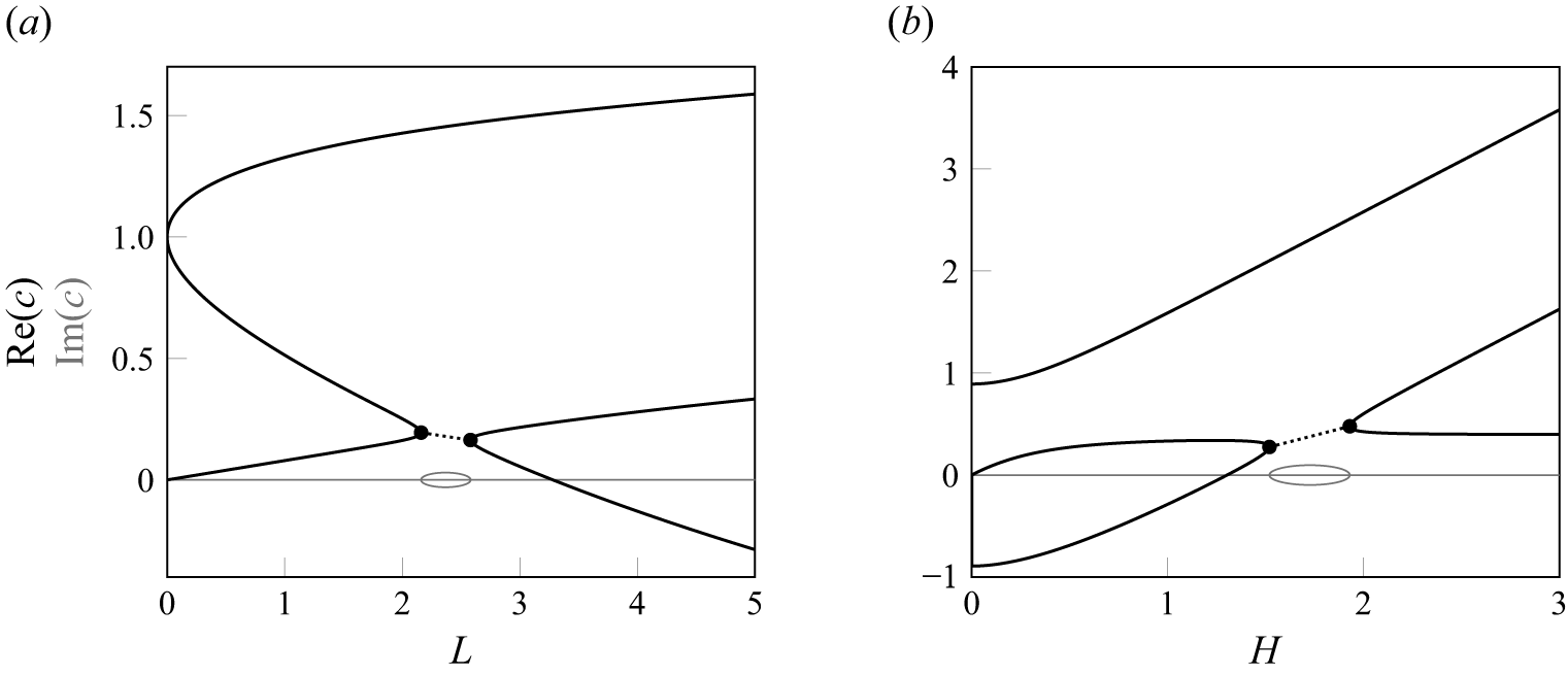
 H=1
 (a)
 L=5
 (b)
 [c]
 [c]
 [c]>0
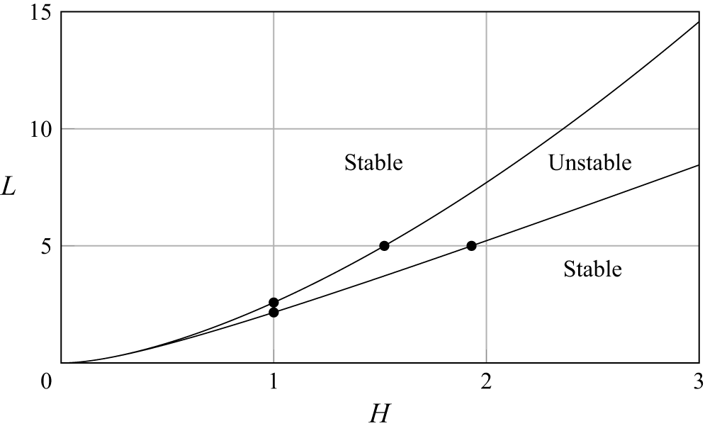
 H
 L
 ζ1(x,t)=H
 ζ2(x,t)=0
 c
 n=1

 (H,c)
 L=5
 n=1
 A=10−5
 c1=(1−e−2kH)/(2k)
 ζ1(x)=0
 c2=H
 ζ2(x)=0
 (a)
 (i)
 ζ1(x)
 ζ2(x)
 ζ1−H
 c

 (H,c)
 L=5
 A=10−5
 n=1
 n
 n=2
 n=3

 (x,y)
 (ξ,η)
 −∞
 ζ2⩽y⩽ζ1
 γ(ξ,t)
 η=0

 A=0.03
 L=5
 N=80
 H,c
 n=1
 (b)

 (a)
 A=0.03
 L=5
 N=80
 n=1
 n=3
 b
 c
 (H,c)
 (a)
 ζ1(x)
 ζ2(x)
 y

 (a)
 A=0.03
 L=5
 N=80
 n=1
 n=3
 b
 c
 (H,c)
 (a)
 ζ1(x)
 ζ2(x)
 y

 (a)
 A=0.03
 L=5
 N=80
 n=1
 n=2
 b
 c
 (H,c)
 (a)
 ζ1(x)
 ζ2(x)
 y

 (a)
 A=0.03
 L=5
 N=80
 n=1
 n=2
 b
 c
 (H,c)
 (a)
 ζ1(x)
 ζ2(x)
 y

 L=5
 N=100
 ζ1(x)
 ζ2(x)
 (a
 i)
 (a,d,f)
 H=0.5
 (c,g,i)
 H=2.5
 A
 aN
 bN
 cN
 dN
 10−10
 c
 P
 E

 c
 P
 E

 ψ^1
 ψ^2
 (ψ^1)
 (ψ^1)
 [max(ψ^1)−min(ψ^1)]/11

 ζ1(x)
 am
 ζ2(x)
 cm
 exp(−36(1.2m/N)36)
 bm
 (d)
 (i)

 Open access

