1. Introduction
Due to the ongoing global warming and increasing extreme weather events, the Arctic ice caps and glaciers are melting at an accelerated pace, leading to a continual reduction in the sea ice area in the polar and high-latitude regions. According to observations, statistics and analyses by the National Aeronautics and Space Administration (NASA), the multi-year sea ice area in 2023 has melted by more than 95% compared with 1984 (Steve and Rani, Reference Steve and Rani2015). NASA has also predicted that by 2050, Arctic Sea ice will completely disappear. The new opportunities presented by the development of polar shipping routes bring new efficiency and safety challenges for various vessels. Fixed ice and floating ice on the water surface, harsh meteorological conditions, and the unpredictability and difficulty in detecting uncertainties during navigation severely affect the navigation of ships and the operational safety of crew members. This makes navigation in high-latitude and frigid polar regions one of the technical and management challenges in the global maritime industry. Ice region vessels are subjected to a harsh external environment regarding hull structure, mechanical equipment and navigation performance. The lack of navigation experience of the crew also brings more risks. The sector is striving to find safer and more efficient ice region navigation solutions.
The risk assessment and safety management of ice region navigation is an important foundational research area in the field of ice region navigation both domestically and internationally, and traffic safety engineering has always been an important research topic in the entire field of transportation. In the field of polar and ice region navigation, due to the limited practical experience in the past, sparse and scattered data resources, and unclear geopolitical and international policies, the research has been somewhat restricted. Due to the lack of data, most scholars use methods such as Bayesian networks, Analytic Hierarchy Process (AHP) and tree models for qualitative assessment studies. Afenyo et al. (Reference Afenyo, Khan, Veitch and Ming2017) used a Bayesian network to analyse the risks and potential causes of collisions between Arctic navigation vessels and icebergs. Khan et al. (Reference Khan, Khan, Veitch and Ming2018) designed a new object-oriented Bayesian network to address the complexity of learning, building and inference in Bayesian network models, making it easier to reconstruct and enhance interpretability, and applied it to the risk assessment of ice collision in the Northern Sea Route, achieving better results. Zhang et al. (Reference Zhang, Hu and Dai2020) achieved state assessment and prediction of Arctic maritime navigation environment risks based on expert experience and risk entropy, and diffusion theory in the context of sparse navigation and accident data in polar waters. Panahi et al. (Reference Panahi, Ng, Afenyo and Haeri2020) used a Bayesian network combined with AHP to analyse the risk of extreme weather in the Arctic waters on ship navigation. In addition to using probabilistic methods to assess the risk of polar navigation environments, another method is to use quantitative risk analysis (QRA) to assess environmental risks. Fedi et al. (Reference Fedi, Faury and Etienne2020) used the POLARIS risk quantification tool to assess the navigation risk of the Northern Sea Route, revealing the types of risks that ships may face along the route and their probabilities, achieving risk mitigation for ship navigation. Li et al. (Reference Li, Jonas and Rita2020) improved the original POLARIS tool to analyse the sea ice environment risk of the Northeast Passage in the Arctic and designed the shortest safe route based on this. An et al. (Reference An, Ma, Wang, Zhang and Li2022) combined POLARIS to assess the environmental risk of the usual route of the Northeast Passage and identified the key risk segments throughout the voyage. However, according to the research of Xu et al. (Reference Xu, Kim and Haugen2021), there are certain problems in the internal logic of POLARIS’s calculation results and related operational requirements. Similarly, Browne et al. (Reference Browne, Taylor, Veitch, Kujala, Khan and Smith2020) also found such problems and made some improvements to the POLARIS system. These theoretical models can make reasonable quantitative assessments of risk situations based on the experience and cognition of experts with a small amount of data support. Admittedly, these methods will reduce the subjectivity of expert cognition through corresponding processing, but it is undeniable that such disadvantages still exist, and it also reduces the credibility and interpretability of the model to some extent.
Empirical analysis and modelling is a data analysis and modelling method based on statistical data, which mainly includes data processing, basic analysis, statistical analysis, modelling and model evaluation. By choosing different models, empirical analysis can support data with different structures, such as cross-sectional data and panel data, and can also be applied to regression analysis in raw data with truncated distribution characteristics, revealing the intrinsic laws and phenomena between data, exploring the mechanisms and factors behind them, and providing support and guidance for decision-making and planning. Empirical analysis and modelling is a flexible model, widely used in geographic information systems, urban planning, environmental management, natural resource management, traffic planning, traffic safety analysis and other fields, and has a wide range of applications in the analysis of waterway transportation accidents.
Weng and others have long been committed to studying the casualties of ship accidents in various waters through empirical analysis methods. In the process of using Logit and Negative binomial regression to study the severity of shipping accidents and mortality surveys, they found a relationship between the severity of accident casualties and spatial location in a binary way (Weng and Yang, Reference Weng and Yang2015). Similar conclusions have been repeatedly confirmed in their studies (Weng et al., Reference Weng, Ge and Han2016, Weng et al., Reference Weng, Yang, Qian and Huang2018). Wang et al. (Reference Wang, Liu, Wang, Graham and Wang2021), in exploring the severity and influencing factors of maritime accidents, found significant correlation results between the severity of accidents and environmental factors such as strong winds and visibility. Similarly, Khan et al. (Reference Khan, Yin, Mustafa and Shi2023) also found a significant impact relationship between weather, environmental factors and berthing accidents in the study of dangerous goods ship berthing accidents. Similarly, Fiskin et al. (Reference Fiskin, Cakir and Sevgili2021) and Sanchez-Varela et al. (Reference Sanchez-Varela, Boullosa-Falces, Larrabe-Barrena and Gomez-Solaeche2021) also employed Logistic regression analysis to investigate the impacts of tugboat accidents and human error during dynamic positioning drilling operations, respectively, demonstrating the broad applicability of these methods in assessing accident risks.
Existing research outcomes have collectively drawn a persuasive inference that a substantial correlation exists between waterway traffic incidents and their respective locations, as well as with external contributing factors. This suggests an inherent linkage between the incidence of such accidents and their geographical locales, which concurrently are influenced by external environmental conditions. Despite these insights offering extremely valuable information and perspectives to the sector, the present empirical analysis research on waterway traffic accidents is not without its limitations. First, the primary focus of these studies often lies in the severity of accidents or casualty rates, which indeed offer valuable references for management authorities. However, for the vessels in operation, what may be of greater concern is the frequency of accidents, or the heterogeneous correlations between incident occurrences and influencing factors. Therefore, the navigation strategy could be adjusted reasonably according to the conclusion of analysis. Second, despite numerous studies identifying the endogenous relationship between accidents and geographical locations, the discourse on spatial effects and clustering characteristics of accidents has not been thoroughly explored. Conclusions are often drawn from a somewhat arbitrary binary classification method, which may not fully capture the complexity of the situation.
It is important to gently point out these limitations, not to undermine the importance of the existing research, but to pave the way for future studies that could further deepen our understanding of waterway traffic accidents. Given the harsh external conditions encountered during navigation in high-latitude ice regions, and the inevitable constraints on communication and rescue resources in practical situations, addressing the aforementioned limitations in the research process becomes even more crucial.
In this paper, we integrate the POLARIS system with multiscale empirical analysis methods to investigate the relationship between navigation accidents and external heterogeneous risks in high-latitude icy waters. A simple yet outstandingly effective quantitative assessment method used in POLARIS for analysing polar navigation risks has been modestly modified to adapt to the calculation of sea ice risk index outcomes (RIOs) under grid data. Considering the inherent deficiencies in the POLARIS system mentioned earlier, we employ a spatial auto-regressive model based on large-scale sea region divisions, and a zero-inflated generalised linear model based on small-scale mesh grid divisions, to collaboratively reanalyse a broader range of external risks, including sea ice, at different observational scales. To validate the effectiveness of the model, degraded general models (including OLS and generalised linear models) are used for indicator verification and comparison. Finally, in terms of model application, to highlight the guidance effect of the analysis results on the navigation strategies of vessels in operation, we use the most conservative method to integrate the results of POLARIS, sea region and mesh grid analyses; based on this risk evaluation value, the comprehensive risk assessment of ice route is carried out. Through the systematic integration of multiple approaches, our research aims to provide concrete recommendations for the safety of shipping in the polar seas, ultimately benefiting ship operators, maritime authorities and policymakers involved in ice region navigation.
In Section 2, the POLARIS system, the ordinary least squares model (OLS), the spatial auto-regressive model (SAM), the generalised linear model and its zero-inflated form are described in detail, which provides the theoretical basis for the subsequent analysis. Section 3 mainly defines the research area, and explains the data sources and cleaning methods. In Section 4, descriptive statistics of accident types and accident years are carried out by basic analysis methods, and it is found that collision and grounding accidents account for a relatively high proportion, and the number of accidents is on the rise. Furthermore, different regression models were used to conduct multiple regression analysis on different spatial scales to explore the ice area risk under the influence of spatial effects, and, combined with traditional quantitative analysis methods, a comprehensive evaluation model of ice area risk was proposed, and numerical verification analysis was carried out with actual customary routes. Finally, in Section 5, the research results are summarised, including the results of data cleaning and statistical analysis, the influencing factors obtained from different model analysis and the rationality of the comprehensive risk assessment model, and the theoretical value and practical application significance of this study are analysed. The flow chart of this study is shown in Figure 1.
Schematic diagram of the study.

2. Methods
2.1. POLARIS
The International Maritime Organization (IMO) has incorporated POLARIS (Polar Operational Limits Assessment Risk Index System), which measures ice navigation risk in ice water regions, as a recommended supplement to the Polar Code (IMO, 2015). However, a practical challenge arises as the computational methods of this system are not suitable for grid map scenarios. To address this issue, our research incorporates the concept of grid sea ice homogenisation (Li et al., Reference Li, Jonas and Rita2020), leading to an enhanced equation for calculating ice operation risk (RIO):
 $$RIO = SIC \times RV + 3\left( {10 - SIC} \right),$$
where SIC represents the average sea ice concentration within a grid and RV refers to the ice risk value of the grid, which is related to the ship’s ice class and the thickness of regional sea ice, as detailed in Appendix A. Supported by remote sensing ice condition data, the formula proposed in this study can effectively retain the philosophy of POLARIS and calculate the sea ice risk reasonably.
While POLARIS serves as a valuable tool for assessing the risks associated with navigating through ice-covered regions, it is important to underscore its limitations. For instance, its computation results may lack precision and it may offer contradictory advice. In high-risk operations, POLARIS simultaneously suggests increasing the sailing speed to maintain ship performance while advocating for a rational restraint on speed. In the face of these circumstances, the POLARIS model still requires improvements.
2.2. Ordinary Least Squares model (OLS) and Spatial Autoregressive Model (SAM)
The Ordinary Least Squares (OLS) is the foundation of all multivariate regression analysis models for waterway traffic accidents (Montgomery et al. Reference Montgomery, Peck and Vining2021). This model assumes that the number of accidents occurring in each analysis unit has a linear relationship with its associated influencing factors, i.e. independent variables and covariates. The model can be represented by the following equation:
 $$\boldsymbol y = X\beta + \varepsilon, \;\varepsilon\!\! \ \sim\it N\left( {0,{\sigma ^2}\boldsymbol I} \right),$$
where
 $\boldsymbol y$
is an N-dimensional column vector, representing the number of accidents in each observation analysis unit; and N is the number of observation analysis units. Here,
X
is a covariate matrix with k rows and N columns, where k is the number of covariates input into the model;
B
is a row vector of length k, representing the coefficients of each covariate; and
 $\;\varepsilon $
is the error term, which follows a multivariate normal distribution with an expected value of 0 and a variance of σ
2
I
, where
I
is the identity matrix.
The unbiased estimate of β, denoted as
 $\widehat {\bf \beta} $
, can be obtained using the method of least squares:
 $${\widehat {\bf \beta} = {{\left( {\boldsymbol{X^T}X} \right)}^{\bf- 1}}\boldsymbol{X^T}y.}$$
The Spatial Autoregressive Model (SAM) is an enhanced form of the OLS model that considers spatial lag relationships. It reflects the spatial correlation of the dependent variable, as shown in the following equation:
 $$\matrix{ \boldsymbol{y = X{\bf \beta} + \it \rho \boldsymbol Wy + \varepsilon } \cr \boldsymbol{\varepsilon \it \sim N\left( {0,{\sigma ^2}\boldsymbol I} \right)} \cr }, $$
where W is the spatial weight matrix and ρ is the spatial lag parameter. The SAM can reflect the spatial effects of accidents during the regression fitting process.
For the estimation of this model, using OLS is biased, so the more general method of Maximum Likelihood Estimation (MLE) is used. Its likelihood function is as follows (LeSage and Pace, Reference LeSage and Pace2009):
 $$\matrix{ {LL\left( {{\bf\beta}, \sigma, \rho } \right) = \ln \left| {\boldsymbol I } - \rho {{\boldsymbol W}} \right| - \left( {{N \over 2}} \right)\ln \left( {2\pi } \right) - \left( {{N \over 2}} \right)\ln \left( {{\sigma ^2}} \right)} \cr { - \left( {{1 \over {2{\sigma ^2}}}} \right){{\left( {y - \rho {\boldsymbol Wy} - {\boldsymbol X\beta} } \right)}^{\rm{'}}}\left( {{\boldsymbol y} - \rho {\boldsymbol Wy} - {\boldsymbol X\beta} } \right).} \cr } $$
The estimated values of the covariate coefficient β and its variance σ, denoted as
 $\boldsymbol{\widehat \beta _{ML}}$
and
 $\boldsymbol {\widehat \sigma _{ML}^2}$
, are as follows:
 $$\matrix{ {{{\boldsymbol{\widehat \beta }_{ML}}} = {{\boldsymbol{\widehat \beta }_0}} - \rho {\boldsymbol{\hat \beta }_L}} \cr {{{\boldsymbol{\widehat \beta }_0}} = {{\left( \boldsymbol{X'X} \right)}^{ - 1}}\boldsymbol X'y} \cr {{{\boldsymbol{\widehat \beta }_L}} = {{\left( \boldsymbol {X'X} \right)}^{ - 1}}\boldsymbol X'Wy} \cr } $$
 $$\matrix{ {\boldsymbol {\widehat \sigma _{\it ML}^{\it 2}} = {{{{\left( {{d_{\it 0}} - \it \rho {\boldsymbol d_{\it L}}} \right)}^{\rm{'}}}\left( {{d_{\it 0}} - \it \rho {\boldsymbol d_{\it L}}} \right)} \over N}} \cr {{\boldsymbol d_{\it 0}} = \boldsymbol y - X{{\widehat \beta }_{\it 0}}} \cr {{\boldsymbol d_{\it L}} = \boldsymbol y - X{{\widehat \beta }_{\it L}}} \cr } $$
2.3. Generalised linear model and its zero-inflated form
In practical research, the dependent variable is not a simple continuous variable, but data of various types that follow various distributions. In such cases, generalised linear models (GLMs) are used for regression analysis. The dependent variable in a GLM is linked to the linear regression portion on the right side through an exponential distribution family link function. This allows us to model various types of data, including binary, multinomial, count and continuous data. It can handle data that do not conform to the assumption of normal distribution or where the variance is unrelated to the mean. Therefore, it has great flexibility in practical applications. It can also adapt to specific problems by choosing different link functions and distribution families, making the model more applicable to various research scenarios. In the analysis of waterway traffic accident characteristics, count distribution functions such as the Poisson and negative binomial distributions, used as link functions, often achieve good results in regression, as confirmed by a large number of successful cases.
The Poisson distribution assumption typically assumes that the average number of event occurrences is constant and that there is no correlation between the number of events occurring within a certain period of time. Suppose the count of accidents observed in water area i is
 ${Y_i}$
, if it follows a Poisson distribution:
 $${Y_i}\sim Poisson\left( {{\lambda _i}} \right)$$
Then, the probability mass function is
 $$P\left( {Y = {y_i}} \right) = {{{e^{ - {\lambda _i}}}{\lambda ^{{y_i}}}} \over {{y_i}!}}$$
Connected to the linear regression equation through a log link function, it becomes
 $$\ln \left( {{\lambda _i}} \right) = {\beta _o} + \mathop \sum \limits_k {\beta _k}{x_{ik}}.$$
At times, the dispersion of traffic accident data (where variance exceeds the mean) challenge the assumption of homoscedasticity, thus compromising the suitability of the Poisson model (Hou et al., Reference Hou, Tarko and Meng2018). The Negative Binomial (NB) regression model builds upon the Poisson regression model by introducing a residual term based on the Gamma distribution. This approach aims to address the over-dispersion and heteroscedasticity issues inherent in the Poisson regression model, theoretically resulting in improved performance.
The NB regression model can be equivalently expressed through a Gamma-distributed residual term transformation as follows (Aguero-Valverde, Reference Aguero-Valverde2013):
 $${Y_i}\sim NB\left( {{p_{i,}},r} \right),$$
where
 ${p_{i,}},r$
are model parameters that satisfy
 $${p_i} = {r \over {{\mu _i} + r}},$$
with
 ${\mu _i}$
denoting the expected value of
 ${Y_i}$
. The expectation and variance of
 ${Y_i}$
are
 $$\matrix{ {E\left( {{Y_i}} \right) = {\mu _i} = {{r\left( {1 - {p_i}} \right)} \over {{p_i}}}} \cr {Var\left( {{Y_i}} \right) = {{r\left( {1 - {p_i}} \right)} \over {p_i^2}} = {1 \over r}\mu _i^2 + {\mu _i}} \cr } .$$
The probability density function of the negative binomial distribution is given by
 $$\matrix{ {P\left( {{Y_{it}}{\ =\ y _i}\mid r,{p_i}} \right) = {{{\rm{\Gamma }}\left( {r + {y_i}} \right)} \over {{y_i}! \times {\rm{\Gamma }}\left( r \right)}}{{\left( {{p_i}} \right)}^r}{{\left( {1 - {p_i}} \right)}^{{y_i}}}}\quad\quad\quad\quad\quad\quad \cr {= {{{\rm{\Gamma }}\left( {r + {y_i}} \right)} \over {{y_i}! \times {\rm{\Gamma }}\left( r \right)}}{{\left( {{r \over {{\lambda _i} + r}}} \right)}^r}{{\left( {{{{\lambda _i}} \over {{\lambda _i} + r}}} \right)}^{{y_i}}}} {,r \gt 0,0 \lt {p_i} \lt 1} \cr } $$
and the regression equation is
 $$\ln \left( {{\mu _i}} \right) = {\beta _o} + \mathop \sum \limits_k {\beta _k}{x_{ik}}$$
In analysing water traffic accidents, many observed zeros arise. A two-state model can handle this by dividing data into zero and non-zero counts, each modelled differently for better prediction. Specifically, a zero-inflated model handles the zeros, while a basic count model fits the non-zero data.
Assuming the relationship between the probability
 ${\theta _i}$
of the first state and the covariates is a binary logit relationship (Weng et al., Reference Weng, Ge and Han2016), the link function for the regression equation of the zero-inflated Poisson model is
 $$\matrix{ {logit\left( {{\theta _i}} \right) = ln\left( {{{{\theta _i}} \over {1 - {\theta _i}}}} \right) = \boldsymbol \beta 'X_i^{\rm{'}}} \cr {ln\left( {{\lambda _i}} \right) = \boldsymbol \beta {X_i}} \cr } $$
its probability mass function given by
 $$P\left( {{Y_i} = {y_i}} \right) = {I_i}{\theta _i} + \left( {1 - {\theta _i}} \right)\left( {{{{\rm{exp}}\left( { - {\lambda _i}} \right){{\left( {{\lambda _i}} \right)}^{{y_i}}}} \over {{y_i}!}}} \right)$$
where
 ${I_i}$
is an indicator variable, which equals 1 when
 ${Y_i} = 0$
, and 0 otherwise.
Similarly, the probability mass function for the zero-inflated negative binomial model is
 $$P\left( {{Y_i} = {y_i}} \right) = {I_i}{\theta _i} + \left( {1 - {\theta _i}} \right){{{\rm{\Gamma }}\left( {r + {y_i}} \right)} \over {{\rm{\Gamma }}\left( r \right){\rm{\Gamma }}\left( {{y_i} + 1} \right)}}{\left( {{r \over {r + {\mu _i}}}} \right)^r}{\left( {{{{\mu _i}} \over {r + {\mu _i}}}} \right)^{{y_i}}}$$
The meanings of the parameters are the same as those mentioned earlier and the link function is the same as in the zero-inflated Poisson model.
3. Study area and data acquisition
3.1. Study area
The Baltic Sea, one of the busiest maritime areas in high-latitude regions, is surrounded by Denmark, Estonia, Finland, Germany, Latvia, Lithuania, Poland, Russia, Sweden, and the plains of Northern and Central Europe. It is located between 53°N and 66°N latitude and 10°E and 30°E longitude. The geographical location is shown in Figure 2.
The scope of the Baltic Sea (Image source: Wikipedia).

Up to 45% of the Baltic Sea is covered by ice annually, presenting significant challenges for navigation, especially in the northern areas. Sea ice reaches its maximum extent in February or March. In the northern basin of the Bothnian Bay and its northernmost regions, the typical ice thickness is approximately 70 cm.
3.2. Data acquisition
After fully considering the climate and sea conditions in the Baltic Sea region and the research results of predecessors, to carry out accident modelling and prediction analysis of macro cross-sectional data and micro panel data, respectively, according to the research needs and the existing data situation, this paper selects the following variables as research variables, which are divided into three categories.
-
1. Accident individual characteristics: records of accidents, types of vessels, size of vessels, meteorological conditions at the time of the accident.
-
2. Macro-regional attribute features: the number of ports in the region, the average daily water traffic flow in the region.
-
3. Micro-water area attribute features: the annual average meteorological conditions in the water area, the annual average traffic flow in the water area.
The subsequent macro-scale analysis and micro-scale analysis are based on the classification of variables in categories 2 and 3. The macro-scale is based on the reasonable division of the actual water body on the geographical scale, and the micro-scale unifies the meteorological data and traffic flow data from different sources to the most detailed spatial resolution to retain the most features.
The meteorological conditions include five items: sea ice concentration, sea ice thickness, sea ice flow speed, seawater flow speed and seawater temperature.
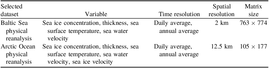
The collection method for meteorological data is to download it through the CMEMS open-source platform. To achieve batch and rapid downloading and to accurately collect meteorological data at the spatiotemporal points of accidents, this paper uses the Python API interface MotuClient provided by CMEMS to manage and organise the data downloading process. The selected datasets and their attributes are shown in Table 1.
CMEMS selected dataset and data attributes

The accident data, traffic flow data and port location data for the region are downloaded from the online map system hosted by the Baltic Marine Environment Protection Commission/Helsinki Commission (HELCOM). The website is https://maps.helcom.fi/website/mapservice/index.html. The downloaded datasets are shown in Table 2.
HELCOM obtained datasets

After resampling, taking the sea ice concentration of different datasets as an example, we can achieve correct coordinate projection transformation and visualisation of meteorological data. To analyse the maritime traffic accidents in the Baltic Sea, we can also correctly project and display the traffic flow density. Figure 3a shows the sea ice concentration of the Baltic Sea physical reanalysis dataset, Figure 3b shows the Baltic Sea region sea ice concentration of the Arctic Ocean physical reanalysis dataset and Figure 3c shows the water traffic flow density in the region in 2018.
Visualisation results of multi-source and multi-type datasets in the Baltic Sea.

HELCOM has continuously collected and organised maritime traffic accidents that occurred in the region from 1989 to 2020, totalling 3,164 cases. As mentioned earlier, the time coverage of the traffic flow density survey dataset for this area is from 2006 to 2022. Considering the huge impact of the global COVID-19 pandemic on the shipping industry, and to ensure that the data used in this study is sufficiently wide in time scale and not affected by too old data situations, this paper selects the traffic flow and accident data for the ten years from 2009 to 2018.
First, the main accident information for the study is filtered out based on time, and longitude and latitude information. The time scale is the ten years from 2009 to 2018, and the longitude and latitude coordinates determine the spatial information of the accident. Accidents scattered outside the study area (such as recording errors or inland waterway accidents) are excluded. Then, the accident attribute information is cleaned up. The random forest method is used to fill in missing values. For columns with too many missing values, the attribute column is chosen to be excluded. Finally, the narrative of text-type data attributes (such as ship type) is unified to solve the problem of inconsistent descriptions. Through such processing, 1,522 complete accident observation records from 2009 to 2018 are obtained.
4. Experiments and analysis
4.1. Basic statistics: descriptive statistical analysis results
The accident types are mainly divided into seven categories. These include:
-
1. ships being stranded or trapped in ice and unable to navigate;
-
2. fires or explosions occurring on ships;
-
3. damage to the ship’s mechanical equipment;
-
4. collisions with other ships or obstacles during navigation and damage to the ship’s hull;
-
5. the ship tilting or capsizing;
-
6. pollution caused by the ship;
-
7. other types of accidents on the ship.
In the dataset of 1,522 accidents, the number and proportion of accident types are shown in Figure 4. The maritime accidents in the Baltic Sea ice area are mainly composed of collisions and grounding accidents, the combined proportion of which accounts for 60% of all accident types in the region.
Proportion of accident types.

Looking at the years when the accidents occurred, after basic double-cycle moving average calculations, during this period, the number of accidents is still on the rise. The statistical charts and calculation results are shown in Figure 5. This shows that the maritime accidents in the region still have a quite serious development trend. The ice navigation in the Baltic Sea region has not yet become a quite complete and safe regional water traffic system.
Histogram of accident frequencies within the observed area.

4.2. Results of large-scale analysis: comparison of SAM and OLS
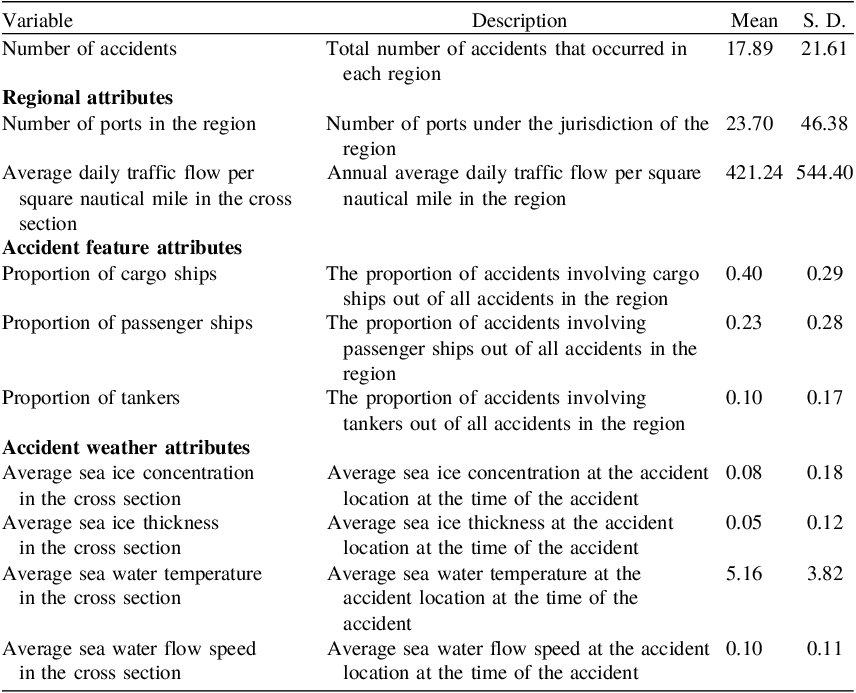
In this study, the dependent variable selected is the number of accidents in the region, which is convenient for probability prediction. In terms of covariate selection, three types of variables are selected, including regional attributes, accident feature attributes and accident environment attributes. All variable selections are shown in Table 3. The spatial division of the observed individuals, namely the results of the L3 level regional division, uses the method of QUEEN contiguity, for the calculation of the spatial adjacency matrix. In this method, the neighbours of a region are defined as those other regions that share a border or vertex with it.
Descriptions and basic statistics of the macro-scale accident data

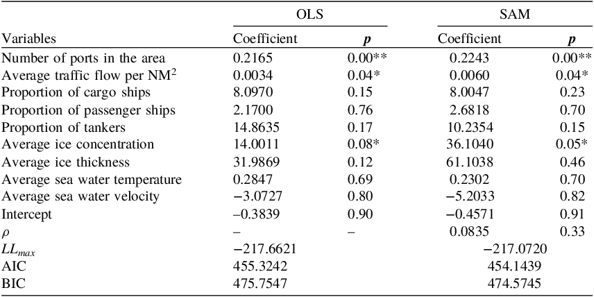
We perform OLS and SAM regression, respectively, and conduct AIC and BIC information criterion tests. AIC (Akaike Information Criterion) and BIC (Bayesian Information Criterion) are two commonly used statistics for model selection. Their main purpose is to strike a balance between model goodness of fit and model complexity to avoid overfitting. Using these criteria, researchers can compare the performance of different models and select the one that is most likely to give the best prediction. In general, a smaller means a better model. The results are shown in Table 4.
Macro-scale model results

**Very significant; *Significant.
The AIC and BIC test values of the SAM model are both smaller than those of the ordinary OLS, proving that the model considering spatial effects is indeed more effective. For regional accident numbers, the number of ports in the area, the average traffic flow per square nautical mile and the ice concentration in the area are all significantly high (p ≤ 0.1), with the number of ports in the area having a very significant impact on the number of accidents. For every additional five ports in the area, the number of accidents in the area will increase by 1. When the traffic flow per square nautical mile in the area increases by 1000, the number of accidents will increase by 6. Additionally, for every 1% increase in ice concentration, the number of accidents increases by 0.3.
Although other indicators are not highly significant, from the perspective of ship types, compared with all other types of vessels, oil tankers have the highest probability of accidents, followed by cargo ships. Passenger ships also increase the probability of accidents, which means that small vessels such as fishing boats, service ships and tugboats have a lower probability of accidents. Among the meteorological indicators, the overall sea ice thickness in the region has a relatively large positive correlation with accidents. This reflects that a harsher overall sea ice environment in the region results in a higher risk of accidents.
4.3. Results of micro-scale analysis: comparison of GLMs and their zero-inflated forms
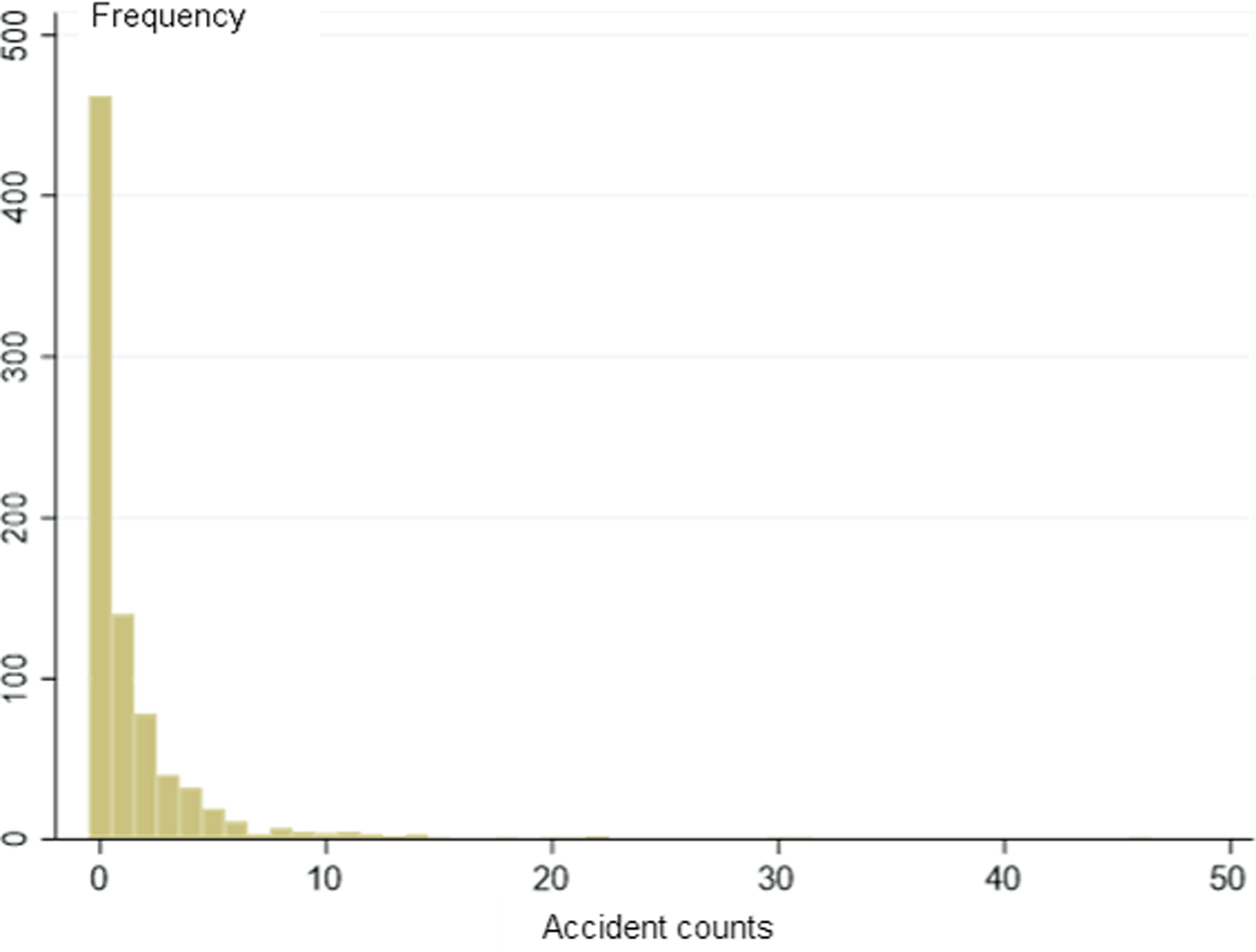
To determine the zero-inflation situation of the panel data, the observation results of each individual observation are plotted in a frequency histogram, as shown in Figure 6. The distribution of zero values is quite prominent and the original data set has a zero-inflation phenomenon, making the model applicable.
Histogram of accident frequencies within the observed area.

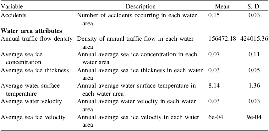
The data used for the micro-scale analysis are shown in Table 5. All the data used here are statistical results and average results at the panel scale, i.e. the number of accidents is the number of accidents in a certain observation year in the study, and the traffic flow and meteorological attributes of the waters are also the statistical results and average results of that year.
Description and Basic statistics of micro-scale accident data

For the two-state model, when AIC, BIC and other standard criteria are used to compare with the standard model, the model’s merits and demerits cannot be accurately judged. At this time, the applicability of the model can be evaluated by the Vuong test (Vuong, Reference Vuong1989). The Vuong statistical test is calculated as follows:
 $$V = {{\bar m\sqrt N } \over {{S_m}}}$$
where
 $\bar m$
and
 ${S_{}}$
are the mean and variance of
 ${m_i}$
respectively, and
 ${m_i}$
is
 $${m_i} = {\rm{ln}}\left[ {{{{{\widehat {{\rm{Pr}}}}_1}\left( {{y_i}\mid {\mu _i}} \right)} \over {{{\widehat {{\rm{Pr}}}}_2}\left( {{y_i}\mid {\mu _i}} \right)}}} \right],$$
where
 ${\widehat {{\rm{Pr}}}_1}\left( {{y_i}\mid {\mu _i}} \right)$
represents the predicted probability of the two-state model and
 ${\widehat {{\rm{Pr}}}_2}\left( {{y_i}\mid {\mu _i}} \right)$
represents the predicted probability of the standard model. If the test value is greater than 1.96, it indicates that the two-state model is superior. If the test value is less than –1.96, it indicates that the standard model is superior. If V takes other values, it means that the superiority between the improved two-state model and the standard model is not significant.
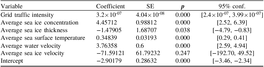
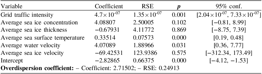
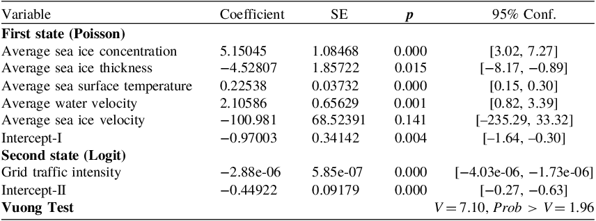
Poisson, NB, ZIP and ZINB regression were carried out, and the information criterion test was conducted. The results are shown in Tables 6, 7, 8, 9 and 10.
Results of micro-scale accident Poisson regression

Results of micro-scale accident NB regression

Results of micro-scale accident ZIP regression

Results of micro-scale accident ZINB regression

Information criterion test of micro-scale accident regression models

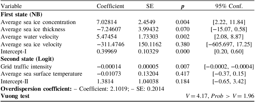
Based on the Vuong test statistics from Tables 8 and 9, it is evident that both types of two-state models have achieved better predictive accuracy, confirming the effectiveness of the models designed in this section, thereby indicating the necessity of using two-state models to address the regression problem of micro-accidents. Furthermore, as indicated by Table 10, the use of the Zero-Inflated Negative Binomial (ZINB) model produces superior results compared with the Zero-Inflated Poisson (ZIP) model.
As shown in Table 9, factors that significantly impact the probability of micro-scale accident occurrences (p < 0.1) include sea ice concentration, sea ice thickness and water current velocity – with particular emphasis on the significant impact of concentration and current velocity. Specifically, for each 1% increase in sea ice concentration, the likelihood of accidents increases by 0.07%, while each 1 m/s rise in water current velocity results in a 0.05% increase in accident probability. Notably, unlike the findings from macro-scale analysis, in the process of micro-scale analysis, sea ice thickness demonstrates a negative correlation to accident probability. This can be attributed to the fact that in the macro-scale analysis process, the meteorological features represent the atmospheric conditions within which the individual accident vessel operates, and the analysis subject primarily focuses on the severity of the regional meteorological conditions. Consequently, more severe sea ice thickness conditions indeed elevate accident risks.
Conversely, in the micro-analysis process, sea ice thickness is an attribute of individual accident entities. Under clear regulations governing vessel entry and navigation standards, water areas with high sea ice thickness witness minimal vessel traffic, especially for operators who rely more on direct observations of sea ice thickness compared with sea ice concentration. These reasons collectively lead to a lower probability of vessels entering areas with relatively high sea ice thickness, resulting in a notably negative correlation effect of sea ice thickness during the micro-analysis process. This underscores the importance of a comprehensive consideration of both macro and micro aspects to obtain a more complete understanding of the various relationships between features and accident probabilities.
4.4. Integrated risk assessment: case studies combining actual ship routes
To quantitatively characterise the risk along an entire route, this paper proposes a comprehensive risk assessment model that integrates the POLARIS RIO risk index, the macro-level risk index provided by the SAM model and the micro-level risk index provided by the ZINB model. The model, rooted in a conservative approach, evaluates the overall risk of a route by considering the maximum values derived from these three models (as RIO operates on an inverse scale where higher values correspond to lower risk, with the maximum value being 30, the calculation of the standard risk value using RIO* involves the formula 30-RIO):
 $$RISK\left( R \right) = \mathop \sum \limits_{{p_i} \in R} \max \left\{ {RI{O^\ast}\left( {{p_i}} \right),SA{M^\ast}\left( {{p_i}} \right),ZIN{B^\ast}\left( {{p_i}} \right)} \right\}$$
In the given equation, R represents a specific route,
 ${p_i}$
denotes all the pixel grid points traversed by the route, and RIO*(), SAM*(), ZINB*() represent the normalised results of the respective calculation operators for each index. Considering the given route R, with the starting point as S and the destination point as T, the relationship between R and
 $\;{p_i}\;$
can be expressed as follows:
 $$R = \left\{ {S,{p_1},{p_2}, \ldots, {p_n},T} \right\}$$
The normalisation for each index is given by
 $${f^*}\left( {{p_i}} \right) = {{f\left( {{p_i}} \right)} \over {\sum f\left( {{p_i}} \right)}}$$
Here,
 ${f^*}\left( {{p_i}} \right)$
represents the standardised risk operator for each grid point. Its value is the ratio of the calculated original value to the risk calculation results along the entire route. This approach effectively resolves the issue of inconsistent measurement scales across different model outcomes.
We consider a case study of the Luleå–Oulu route. Luleå and Oulu are two major ports in the northernmost part of the Baltic Sea’s Gulf of Bothnia. Luleå port (65.5°N, 22.4°E) is located on the western coast of the Gulf of Bothnia and belongs to Sweden, while Oulu port (65°N, 25.12°E) is situated on the eastern coast and belongs to Finland. The route is illustrated in Figure 7.
The Gulf of Bothnia: Luleå–Oulu route.

The departure, arrival and turning waypoints along the route are provided in Table 11. The arrival position for Oulu port corresponds to its proximity location.
The Luleå–Oulu route and its waypoints

The risk visualisation maps for the RIO* model, the SAM model and the ZINB model are depicted as Figures 8, 9 and 10, where darker shades indicate higher risks. Based on publicly available reports, most ships entering the northern Baltic Sea opt for IA ice-class vessels. In this study, the analysed vessel is a General Cargo ship with an IA ice class, and the meteorological conditions correspond to a certain day in November 2023. It is evident that the different models identify varying levels of risk, displaying distinct spatial distributions. However, they generally indicate lower risk towards the southern end of the area, with an observable increase in risk closer to the coastline.
RIO* risk map.

SAM risk map.

ZINB risk map.

The route is discretised into pixels at the most delicate meteorological data source scale, and then the indicators are standardised. The results are shown in Figure 11.
Risk assessment model outputs standardised risk values.

As illustrated in Figure 12, the area plots of the standardised risk values from the three models are presented on a unified coordinate system, revealing distinctive traits for each. The improved RIO model based on POLARIS notably identifies heightened navigational risks near the port of Oulu. This aligns with the practical conditions, as the waters near Oulu predominantly contain consolidated pack ice during winter, necessitating icebreaker escort for entry, thereby validating the model’s reliability. However, the RIO model exhibits poorer risk identification in areas with floating ice, indicating a generally higher tolerance for risk during most navigation processes. The SAM model demonstrates a strong capability in recognising risks during the segment of navigation post-departure or pre-arrival, actively factoring in spatial relationships when analysing accident risks, enabling the detection of high-risk navigation behaviours within 20 nautical miles of the coastline. As a risk analysis method based on water area partitioning, the ZINB model more effectively responds to meteorological variations. In comparison to the other two models, its risk identification results tend towards smoother trends, yet it dynamically achieves meteorological risk detection, serving as a fundamental reference for risk modelling.
Relative area proportions of different risk assessment models.

The comprehensive risk identification results are illustrated in Figure 13.
Comprehensive risk identification findings.

5. Conclusion
The study focuses on the Baltic Sea waters, conducting data cleaning and basic statistics on the acquired data. It is observed that the maritime risk in this region is likely to be associated with varying meteorological conditions at different times and spatial clustering of accidents. To validate these conclusions drawn from basic statistical methods, the study sets up a large-scale regression model to analyse spatial correlations, as well as a small-scale regression model that addresses issues related to a substantial number of zero values and places emphasis on analysing the relationship with meteorological conditions at different times. The findings demonstrate that the SAM model using spatial correlation achieves better model accuracy compared with the OLS model. Furthermore, the ZINB distribution provides a better fit to the data in comparison to the ZIP, Poisson and NB distributions. The results indicate a significant impact of the number of ports in each Baltic Sea region on the number of accidents. For each increase of five ports within a region, the number of accidents increases by 1. Additionally, for every 1,000 square nautical miles increase in traffic flow within a region, the number of accidents rises by 6. Moreover, a 1% increase in sea ice density leads to a 0.3 increase in accidents. For a specific vessel, a 1% rise in surrounding sea ice density results in a 0.07% increase in the probability of an accident occurring, and for every 1 m/s increase in seawater flow velocity, there is a 0.05% increase in accident probability. Based on the analysis of different scale models, the comprehensive risk assessment model proposed aligns with current normative risk assessment methods, and can achieve robust identification of navigation risks in various stages, spatial characteristics and meteorological features. It demonstrates a certain degree of reasonableness in conservative risk estimation models compared with current norms.
At a theoretical level, the study emphasises the theoretical value and practical application of ship-oriented analysis in ice-infested waterway accidents. Furthermore, it highlights the spatial effects and external environmental impacts in maritime accident analysis, both of which play a crucial role in the causes and consequences of accidents. The spatial effect emphasises how geographic location and environmental conditions influence accident occurrences, while the external environmental effect focuses on the role of factors such as climate change and ice conditions in accidents. This theoretical framework not only helps us to further understand the complexity of ice-infested maritime accidents, but also provides new perspectives and strategies for preventing and addressing such accidents.
It is expected that the authorities or aircrews can use the method proposed in this paper to use the forecast meteorological data for sea ice risk estimation and make early warnings or adjust routes, providing more considered risk classification results than the POLARIS method in different space environments. To take the research further, we will try to fuse the two-scale risk analysis model, consider the spatial effect and the large number of zero value problems at the same time, and construct a comprehensive zero-inflated geographically weighted generalised linear regression model to analyse the navigation risk in an ice region.
Funding statement
This work was supported by the National Key Research and Development Program of China (Grant No. 2021YFC2801000), National Natural Science Foundation of China (Grant No. 52071199) and Shanghai Science and Technology Innovation Action Plan (Grant Nos. 22DZ1204503).
Appendix A. Sea ice risk value