2.1 General formalism

Here, we recall the basics of the spin Vlasov–Maxwell system in the extended phase space (Marklund et al. Reference Marklund, Zamanian and Brodin2010; Zamanian et al. Reference Zamanian, Marklund and Brodin2010a; Marklund & Morrison Reference Marklund and Morrison2011; Manfredi et al. Reference Manfredi, Hervieux and Hurst2019), satisfied by the scalar electron distribution function:

(2.1)\begin{equation} f:(t, {\boldsymbol x}, {\boldsymbol p}, {\boldsymbol s})\in \mathbb{R}_+{\times} \mathbb{R}^3\times \mathbb{R}^3\times \mathbb{R}^3 \mapsto f(t, {\boldsymbol x}, {\boldsymbol p}, {\boldsymbol s}) \in \mathbb{R}, \end{equation}

and the self-consistent electromagnetic fields $({\boldsymbol E}, {\boldsymbol B}): (t, {\boldsymbol x})\mapsto ({\boldsymbol E}, {\boldsymbol B})(t, {\boldsymbol x})\in \mathbb {R}^3\times \mathbb {R}^3$. The spin Vlasov–Maxwell equations read as

(2.2)\begin{align} \left. \begin{gathered} \frac{\partial f}{\partial t}+\frac{{\boldsymbol p}}{m}\boldsymbol{\cdot} \boldsymbol{\nabla} f+\left[q\left({\boldsymbol E}+\frac{{\boldsymbol p}}{m}\times{\boldsymbol B}\right) +\mu_e\boldsymbol{\nabla}({\boldsymbol s} \boldsymbol{\cdot} {\boldsymbol B})\right]\boldsymbol{\cdot}\frac{\partial f}{\partial{\boldsymbol p}} + \frac{2\mu_e}{\hbar} ({\boldsymbol s}\times {\boldsymbol B}) \boldsymbol{\cdot} \frac{\partial f}{\partial {\boldsymbol s}}=0,\\ \epsilon_0 \mu_0 \frac{\partial{\boldsymbol E}}{\partial t}=\boldsymbol{\nabla}\times{\boldsymbol B}-\mu_0{\boldsymbol J},\\ \frac{\partial{\boldsymbol B}}{\partial t} ={-} \boldsymbol{\nabla}\times{\boldsymbol E},\\ \boldsymbol{\nabla}\boldsymbol{\cdot}{\boldsymbol E}=\frac{\rho-q n_0}{\epsilon_0},\\ \boldsymbol{\nabla}\boldsymbol{\cdot}{\boldsymbol B}=0, \end{gathered} \right\} \end{align}

In the original paper on the scalar spin Vlasov equation (Zamanian et al. Reference Zamanian, Marklund and Brodin2010a), one further term was present, which has the form of a modified quantum magnetic dipole term:

(2.3)\begin{equation} \mu_e \left[ \boldsymbol{\nabla}\left({\boldsymbol B} \boldsymbol{\cdot} \frac{\partial}{\partial {\boldsymbol s}}\right) \right] \boldsymbol{\cdot}\frac{\partial f}{\partial{\boldsymbol p}} . \end{equation}

In subsequent works by the same authors, this term was often ignored because of the semiclassical approximation made there (Brodin et al. Reference Brodin, Marklund, Zamanian, Ericsson and Mana2008, Reference Brodin, Marklund, Zamanian and Stefan2011; Brodin & Stefan Reference Brodin and Stefan2013). This can be justified by assuming that variations of $f$ in spin space are of moderate size (for a more detailed discussion, see Zamanian et al. Reference Zamanian, Marklund and Brodin2010a; Brodin et al. Reference Brodin, Marklund, Zamanian and Stefan2011). It should also be pointed out that this modified quantum dipole term contains derivatives in both real and spin space, thus making the PIC algorithm much more involved. For these reasons, such an extra term is neglected in the present developments and will be left to future works on this topic.

The coupling between the Vlasov and Maxwell equations is ensured by the current and the density $({\boldsymbol J}, \rho ) : (t, {\boldsymbol x})\mapsto ({\boldsymbol J}, \rho )(t, {\boldsymbol x})\in \mathbb {R}^3\times \mathbb {R}_+$, defined respectively as

(2.4)\begin{equation} {\boldsymbol J} = q \int_{\mathbb{R}^6} {\boldsymbol p}f \,\mathrm{d}{\boldsymbol p}\,\mathrm{d}{\boldsymbol s} + {\mu_e} \boldsymbol{\nabla} \times \int_{\mathbb{R}^6} {\boldsymbol s} f \,\mathrm{d}{\boldsymbol p}\,\mathrm{d}{\boldsymbol s}, \quad \rho = q \int_{\mathbb{R}^6} f \,\mathrm{d}{\boldsymbol p}\,\mathrm{d}{\boldsymbol s}. \end{equation}

Here, $q = -e$ is the electron charge, $\mu _e = {q\hbar }/{2m}$ is the Bohr magneton, $\hbar$ is the Planck constant, $m$ is the electron mass, $n_0$ is the fixed ion density, and $\epsilon _0, \mu _0$ denote the permittivity and the permeability of vacuum (which satisfy $\epsilon _0 \mu _0 = c^{-2}$, with $c$ being the speed of light). We further note that, in this model, the spin vector ${\boldsymbol s}$ is dimensionless and has fixed length, i.e. $|{\boldsymbol s}| = 1$ or ${\boldsymbol s} \in \mathbb {S}^2$. Hence, the effective phase space is actually 8-dimensional. However, to preserve the geometric structure that will be used in the forthcoming sections, we will consider that ${\boldsymbol s} \in \mathbb {R}^3$.

In the above Vlasov equation (2.2), the first three terms are the standard terms present in the spin-less case, the next term [$\boldsymbol {\nabla }({\boldsymbol s}\boldsymbol {\cdot } {\boldsymbol B})$] is the Zeeman effect and the last term (${\boldsymbol s} \times {\boldsymbol B}$) represents the spin precession in the magnetic field. In (2.4), the second term in the current represents the curl of the internal magnetization owing to the electron spin. Further details can be found in the paper by Manfredi et al. (Reference Manfredi, Hervieux and Hurst2019).

We shall use normalized units, denoted by a tilde and defined as follows:

(2.5a–f)\begin{align} \frac{t}{1/\omega_p} = \tilde{t}, \quad \frac{\boldsymbol x}{\lambda} = \tilde{\boldsymbol x},\quad \frac{\boldsymbol p}{mc} = \tilde{\boldsymbol p},\quad \frac{f}{n_0/c^3} = \tilde{f}, \quad \frac{\boldsymbol E}{{\omega_p c m/|q|}} = \tilde{\boldsymbol E},\quad \frac{\boldsymbol B}{{\omega_p m/|q|}} = \tilde{\boldsymbol B}, \end{align}

where we introduce the electron plasma frequency, the plasma skin depth and the scaled Planck constant:

(2.6a–c)\begin{equation} \omega_p = \sqrt{\frac{n_0 q^2}{m \epsilon_0}}, \quad \lambda = \frac{c}{\omega_p}, \quad {\mathfrak{h}} = \frac{ \hbar \omega_p}{2 m c^2}. \end{equation}

The dimensionless version of (2.2) reads as

(2.7)\begin{equation} \left. \begin{gathered} \frac{\partial f}{\partial t}+{\boldsymbol p}\boldsymbol{\cdot} \boldsymbol{\nabla} f+[\left({\boldsymbol E}+{\boldsymbol p}\times{\boldsymbol B}\right) + {\mathfrak{h}} \; \boldsymbol{\nabla}({\boldsymbol s} \boldsymbol{\cdot} {\boldsymbol B})]\boldsymbol{\cdot}\frac{\partial f}{\partial{\boldsymbol p}} + ({\boldsymbol s}\times {\boldsymbol B}) \boldsymbol{\cdot} \frac{\partial f}{\partial {\boldsymbol s}}=0,\\ \frac{\partial{\boldsymbol E}}{\partial t}= \boldsymbol{\nabla}\times{\boldsymbol B}- \int_{\mathbb{R}^6} {\boldsymbol p}f \,\mathrm{d}{\boldsymbol p}\,\mathrm{d}{\boldsymbol s} + {\mathfrak{h}} \; \boldsymbol{\nabla} \times \int_{\mathbb{R}^6} {\boldsymbol s} f \,\mathrm{d}{\boldsymbol p}\,\mathrm{d}{\boldsymbol s},\\ \frac{\partial{\boldsymbol B}}{\partial t} ={-} \boldsymbol{\nabla}\times{\boldsymbol E},\\ \boldsymbol{\nabla}\boldsymbol{\cdot}{\boldsymbol E}={\int_{\mathbb{R}^6} f\,\mathrm{d}{\boldsymbol p}\,\mathrm{d}{\boldsymbol s} -1},\\ \boldsymbol{\nabla}\boldsymbol{\cdot}{\boldsymbol B}=0, \end{gathered} \right\} \end{equation}

where we remove the tilde to simplify the notation. The above dimensionless version of the spin Vlasov–Maxwell model will be used throughout this work.

It has been shown by Marklund & Morrison (Reference Marklund and Morrison2011) that (2.7) enjoys a non-canonical Poisson structure that enables us to rewrite this complex system in a more compact way. Let us denote $\mathcal{M}=\{(f, {\boldsymbol E},{\boldsymbol B})|\,\boldsymbol {\nabla }\boldsymbol {\cdot }{\boldsymbol B}=0\}$ as the infinite dimensional manifold. The system (2.7) can be expressed using the Poisson bracket introduced by Marklund & Morrison (Reference Marklund and Morrison2011). For two functionals $(\mathcal {F}, \mathcal {G})$ acting on ${\mathcal {M}}$, we consider the following Poisson bracket, which is the sum of the Vlasov–Maxwell bracket (Marsden & Weinstein Reference Marsden and Weinstein1982) and a bracket describing spin effects:

(2.8)\begin{equation} \left. \begin{aligned} \{\mathcal{F},\mathcal{G}\}& = \{\mathcal{F}, \mathcal{G}\}_{\textrm{VM}} + \{ \mathcal{F}, \mathcal{G}\}_{s}, \quad \text{with }\\ \{ \mathcal{F}, \mathcal{G}\}_{\textrm{VM}} & = \int_{\mathbb{R}^9} f\left[\frac{\delta\mathcal{F}}{\delta f},\frac{\delta\mathcal{G}} {\delta f}\right]_{\boldsymbol{xp}}\,\mathrm{d}\boldsymbol{x}\,\mathrm{d}\boldsymbol{p}\,\mathrm{d}\boldsymbol{s}\\ & \quad +\int_{\mathbb{R}^9} \left(\frac{\delta\mathcal{F}}{\delta\boldsymbol{E}}\boldsymbol{\cdot}\frac{\partial f}{\partial\boldsymbol{p}}\frac{\delta\mathcal{G}}{\delta f}-\frac{\delta\mathcal{G}}{\delta\boldsymbol{E}}\boldsymbol{\cdot}\frac{\partial f}{\partial\boldsymbol{p}}\frac{\delta\mathcal{F}}{\delta f}\right)\,\mathrm{d}\boldsymbol{x}\,\mathrm{d}\boldsymbol{p}\,\mathrm{d}\boldsymbol{s}\\ & \quad+\int_{\mathbb{R}^3}\left(\frac{\delta\mathcal{F}}{\delta\boldsymbol{E}}\boldsymbol{\cdot}\left(\triangledown\times\frac{\delta\mathcal{G}}{\delta\boldsymbol{B}}\right) -\frac{\delta\mathcal{G}}{\delta\boldsymbol{E}}\boldsymbol{\cdot} \left(\triangledown\times\frac{\delta\mathcal{F}}{\delta\boldsymbol{B}}\right)\right)\,\mathrm{d}\boldsymbol{x}\\ & \quad +\int_{\mathbb{R}^9} f{\boldsymbol B}\boldsymbol{\cdot}\left(\frac{\partial}{\partial\boldsymbol{p}}\frac{\delta\mathcal{F}}{\delta f}{\times}\frac{\partial}{\partial\boldsymbol{p}}\frac{\delta\mathcal{G}}{\delta f}\right)\,\mathrm{d}\boldsymbol{x}\,\mathrm{d}\boldsymbol{p}\,\mathrm{d}\boldsymbol{s},\\ \{ \mathcal{F}, \mathcal{G}\}_{s} & = \frac{1}{\mathfrak{h}} {\int}_{\mathbb{R}^9} f{\boldsymbol s} \boldsymbol{\cdot} \left(\frac{\partial }{\partial {\boldsymbol s}}\frac{\delta \mathcal{F}}{\delta f} \times \frac{\partial }{\partial {\boldsymbol s}} \frac{\delta \mathcal{G}}{\delta f}\right)\,\mathrm{d}\boldsymbol{x}\,\mathrm{d}\boldsymbol{p}\,\mathrm{d}\boldsymbol{s}. \end{aligned} \right\} \end{equation}

Here, $[\boldsymbol {\cdot },\boldsymbol {\cdot }] _{\boldsymbol {xp}}$ denotes the Lie bracket for two functions of $({\boldsymbol x},{\boldsymbol p})$. It was proven by Marklund & Morrison (Reference Marklund and Morrison2011) that the bracket (2.8) is indeed a Poisson bracket. With the Hamiltonian functional defined as follows:

(2.9)\begin{align} \mathcal{H}(f,\boldsymbol{E},\boldsymbol{B})=\frac{1}{2}\int_{\mathbb{R}^9} |\boldsymbol{p}{}|^{2}f\,\mathrm{d}\boldsymbol{x}\,\mathrm{d}\boldsymbol{p}\,\mathrm{d}\boldsymbol{s} + {\mathfrak{h}}\int_{\mathbb{R}^9} {\boldsymbol s}\boldsymbol{\cdot} {\boldsymbol B} f\,\mathrm{d}\boldsymbol{x}\,\mathrm{d}\boldsymbol{p}\,\mathrm{d}\boldsymbol{s}+ \frac{1}{2}\int_{\mathbb{R}^3} \left(|\boldsymbol{E}|^{2}+|\boldsymbol{B}|^{2}\right)\,\mathrm{d}\boldsymbol{x}, \end{align}

the spin Vlasov–Maxwell system (2.7) can be written in a compact way, using $\mathcal {Z}:=(f,\boldsymbol {E},\boldsymbol {B})\in \mathcal {M}$:

(2.10)\begin{equation} \frac{\partial{\mathcal{Z}}}{\partial t}=\{\mathcal{Z},\mathcal{H}\}, \end{equation}

where $\{\boldsymbol {\cdot } , \boldsymbol {\cdot }\}$ is given by (2.8). This system is supplemented with an initial condition ${\mathcal {Z}}(t=0)={\mathcal {Z}}_0$.

2.2 Reduced spin Vlasov–Maxwell equations

Here, following Ghizzo et al. (Reference Ghizzo, Bertrand, Shoucri, Johnston, Fijalkow and Feix1990), we derive a reduced spin Vlasov–Maxwell model by considering the case of a plasma interacting with an electromagnetic wave propagating in the longitudinal $x$ direction and assuming that all fields depend spatially on $x$ only. Choosing the Coulomb gauge $\boldsymbol {\nabla } \boldsymbol {\cdot } \boldsymbol A =0$, the vector potential ${\boldsymbol A}$ lies in the perpendicular (transverse) plane, i.e. ${\boldsymbol A} = { (0, A_y, A_z) = }(0, {\boldsymbol A}_\perp$). Using ${\boldsymbol E} = -\boldsymbol {\nabla } \phi - \partial _t {\boldsymbol A}$, we then obtain, using the notations ${\boldsymbol E} = (E_x, E_y, E_z) =(E_x, {\boldsymbol E}_\perp )$:

(2.11)\begin{equation} {\boldsymbol E}_\perp = -\partial_t {\boldsymbol A}_\perp \quad \text{and}\quad E_x={-}\partial_x \phi. \end{equation}

This prescription implies that the electric field is mainly electromagnetic in the transverse plane and mainly electrostatic in the longitudinal direction.

We then consider a distribution function of the form: $\delta (\boldsymbol {p}_\perp - \boldsymbol {A}_\perp ) f(t, x, p_x, \boldsymbol {s})$, where $\boldsymbol {p}=(p_x,p_y,p_z)=(p_x,\boldsymbol {p}_\perp )$ is the linear momentum and $\boldsymbol {p}- \boldsymbol {A}$ is the canonical momentum. The above assumption on the distribution function is tantamount to prescribing that the plasma is cold in the transverse plane. After integration with respect to $\boldsymbol {p}_\perp$, the relevant extended phase space is reduced to five dimensions (instead of nine dimensions for the general case). The longitudinal variable $p_x$ will be simply denoted by $p$ in the rest of this paper.

The reduced spin Vlasov–Maxwell system satisfied by the electron distribution function $f(x, p, {\boldsymbol s}, t)$ ($x, p \in \mathbb {R}$ and ${\boldsymbol s} \in \mathbb {R}^3$), the electric field ${\boldsymbol E}(t, x) = (E_x, {\boldsymbol E}_\perp )(t, x) = (E_x, E_y, E_z)(t, x)$ and the vector potential ${\boldsymbol A}(t, x) = (A_x, {\boldsymbol A}_\perp )(t, x) = (0, A_y, A_z)(t, x)$ can be written as

(2.12)\begin{align} \left. \begin{gathered} \frac{\partial f}{\partial t} + p \frac{\partial f}{\partial x} + \left[ E_x - {\mathfrak{h}} \; s_y \frac{\partial^2 A_z}{\partial x^2} + {\mathfrak{h}} \; s_z \frac{\partial^2 A_y}{\partial x^2} - {\boldsymbol A}_\perp \boldsymbol{\cdot} \frac{\partial {\boldsymbol A}_\perp}{\partial x} \right] \frac{\partial f}{\partial p} + (\boldsymbol{s}\times \boldsymbol{B} )\boldsymbol{\cdot} \frac{\partial f}{\partial {\boldsymbol s}} = 0,\\ \boldsymbol{B} = \boldsymbol{\nabla} \times \boldsymbol{ A} = \left[0, \frac{\partial A_z}{\partial x}, -\frac{\partial A_y}{\partial x} \right]^\mathrm{T},\\ \frac{\partial E_x}{\partial t} ={-}\int_{\mathbb{R}^4} p f \,\mathrm{d}p\,\mathrm{d}{\boldsymbol s},\\ \frac{\partial E_y}{\partial t} ={-} \frac{\partial^2 A_y}{\partial x^2} + A_y \int_{\mathbb{R}^4} f \,\mathrm{d}p\,\mathrm{d}{\boldsymbol s} + {\mathfrak{h}}\int_{\mathbb{R}^4} s_z \frac{\partial f}{\partial x}\,\mathrm{d}p\,\mathrm{d}{\boldsymbol s},\\ \frac{\partial E_z}{\partial t} ={-} \frac{\partial^2 A_z}{\partial x^2} + A_z \int_{\mathbb{R}^4} f \,\mathrm{d}p\,\mathrm{d}{\boldsymbol s} - {\mathfrak{h}} \int_{\mathbb{R}^4} s_y \frac{\partial f}{\partial x}\,\mathrm{d}p\,\mathrm{d}{\boldsymbol s},\\ \frac{\partial {\boldsymbol A}_\perp}{\partial t} ={-} {\boldsymbol E}_\perp,\\ \frac{\partial E_x}{\partial x} = \int_{\mathbb{R}^4} f \,\mathrm{d}p\,\mathrm{d}{\boldsymbol s} - 1. \end{gathered} \right\} \end{align}

This reduced spin Vlasov–Maxwell system also possesses a non-canonical Poisson structure. For any two functionals $\mathcal {F}$ and $\mathcal {G}$ depending on the unknowns $f, {\boldsymbol E}$ and ${\boldsymbol A}_\perp$, the Poisson bracket reads as

(2.13)\begin{gather} \{ \mathcal{F}, \mathcal{G}\} = \int_{\mathbb{R}^5} f\left[\frac{\delta\mathcal{F}}{\delta f},\frac{\delta\mathcal{G}} {\delta f}\right]_{{xp}}\,\mathrm{d}{x}\,\mathrm{d}{p}\,\mathrm{d}\boldsymbol{s} +\int_{\mathbb{R}^5} \left(\frac{\delta\mathcal{F}}{\delta {E_x}}\frac{\partial f}{\partial {p}}\frac{\delta\mathcal{G}}{\delta f}-\frac{\delta\mathcal{G}}{\delta {E_x}}\frac{\partial f}{\partial {p}}\frac{\delta\mathcal{F}}{\delta f}\right)\,\mathrm{d}{x}\,\mathrm{d}{p}\,\mathrm{d}\boldsymbol{s}\nonumber\\ + \int_{\mathbb{R}} \left( \frac{\delta \mathcal{G}}{\delta {\boldsymbol A}_\perp} \boldsymbol{\cdot} \frac{\delta \mathcal{F}}{\delta {\boldsymbol E}_\perp} - \frac{\delta \mathcal{F}}{\delta {\boldsymbol A}_\perp} \boldsymbol{\cdot} \frac{\delta \mathcal{G}}{\delta {\boldsymbol E}_\perp}\right) \,\mathrm{d} x + \frac{1}{\mathfrak{h}}\int_{\mathbb{R}^5} f {\boldsymbol s}\boldsymbol{\cdot} \left( \frac{\partial}{\partial {\boldsymbol s}}\frac{\delta \mathcal{F}}{\delta {f}} \times \frac{\partial}{\partial {\boldsymbol s}}\frac{\delta \mathcal{G}}{\delta {f}} \right) \,\mathrm{d} x\,\mathrm{d}p\,\mathrm{d}{\boldsymbol s}, \end{gather}

whereas the Hamiltonian functional, composed of the sum of kinetic, electric, magnetic and Zeeman (spin-dependent) energies, is defined by

(2.14)\begin{gather} \mathcal{H}(f, {\boldsymbol E}, {\boldsymbol A}_\perp) = \underbrace{\frac{1}{2}\int_{\mathbb{R}^5} p^2 f \,\mathrm{d} x\,\mathrm{d}p\,\mathrm{d}{\boldsymbol s} + \frac{1}{2}\int_{\mathbb{R}^5} |{\boldsymbol A}_\perp|^2 f \,\mathrm{d} x\,\mathrm{d}p\,\mathrm{d}{\boldsymbol s}}_{\text{kinetic energy}}+ \underbrace{\frac{1}{2}\int_{\mathbb{R}} |{\boldsymbol E}|^2 \,\mathrm{d} x}_{\text{electric energy}}\nonumber\\ + \underbrace{\frac{1}{2}\int_{\mathbb{R}} \left|\frac{\partial {\boldsymbol A}_\perp}{\partial x}\right|^2 \,\mathrm{d} x}_{\text{magnetic energy}} + \underbrace{{\mathfrak{h}}\int_{\mathbb{R}^5} \left( s_y \frac{\partial A_z}{\partial x} {-} s_z \frac{\partial A_y}{\partial x} \right) f \,\mathrm{d} x\,\mathrm{d}p\,\mathrm{d}{\boldsymbol s}}_{\text{Zeeman energy}}. \end{gather}

Thus, the reduced spin Vlasov–Maxwell system of (2.12) can be reformulated as

(2.15)\begin{equation} \frac{\partial \mathcal{Z}}{\partial t} = \{ \mathcal{Z}, \mathcal{H} \}, \end{equation}

where $\mathcal {Z}=(f, E_x,E_y,E_z,A_y,A_z)$ denotes the unknowns of the system, $\{\boldsymbol {\cdot }, \boldsymbol {\cdot } \}$ is defined by (2.13) and the Hamiltonian $\mathcal {H}$ is given by (2.14). In this work, periodic boundary conditions will be considered in the $x$ and ${\boldsymbol s}$ directions ($x\in [0, L], L>0, {\boldsymbol s}\in \mathbb {R}^3$), and vanishing boundary condition in $p \in \mathbb {R}$. An initial condition ${\mathcal {Z}}(t=0)={\mathcal {Z}}_0=(f_0, {\boldsymbol E}_{0}, {\boldsymbol A}_{\perp , 0})$ supplements the system. The Poisson bracket (2.13) can be derived from (2.8) using chain rules of functional derivatives based on a similar change of unknowns proposed by Li et al. (Reference Li, Sun and Crouseilles2020).

3.1 Derivation of the discrete Poisson bracket

Using the above approximation of the electromagnetic fields (3.8)–(3.9) and of the distribution function (3.10), we shall construct a discrete geometric structure (discrete Poisson bracket and discrete Hamiltonian) from which the equations of motion will be derived. Specifically, discrete functional derivatives are derived based on the discrete representation of the unknowns (3.8)–(3.9) (see Appendix A for more details), which are inserted into the continuous Poisson bracket (2.13) to derive the discrete Poisson bracket.

We introduce some notations to make the expressions simpler. First, we introduce the discrete time-dependent unknowns for the electromagnetic fields:

(3.11)\begin{align} \left. \begin{gathered} {\boldsymbol{e}}_x \!=\! (e_{x,1}, \ldots, e_{x,N_1})^{\mathrm{T}}\in \mathbb{R}^{N_1}, \ {\boldsymbol{e}}_y \!=\! (e_{y,1}, \ldots, e_{y,N_0})^{\mathrm{T}}\in \mathbb{R}^{N_0},\ {\boldsymbol{e}}_z \!=\! (e_{z,1}, \ldots, e_{z,N_0})^{\mathrm{T}}\in \mathbb{R}^{N_0},\\ {\boldsymbol{a}}_y = (a_{y,1}, \ldots, a_{y,N_0})^{\mathrm{T}}\in \mathbb{R}^{N_0},\ {\boldsymbol{a}}_z = (a_{z,1}, \ldots, a_{z,N_0})^{\mathrm{T}}\in \mathbb{R}^{N_0}, \end{gathered} \right\} \end{align}

and for the particles (position, velocity and spin):

(3.12)\begin{equation} \left. \begin{gathered} {\boldsymbol{X}} = (x_1, \ldots, x_{N_p})^{\mathrm{T}}\in \mathbb{R}^{N_p},\ {\boldsymbol{P}} = (p_1, \ldots, p_{N_p})^{\mathrm{T}}\in \mathbb{R}^{N_p},\\ {\boldsymbol{S}}_i = (s_{1,i}, \ldots, s_{a,i}, \ldots, s_{N_p,i})^{\mathrm{T}}\in \mathbb{R}^{N_p},\ i \in \{x, y, z \},\\ {\boldsymbol{S}} = ({\boldsymbol s}_{1}, {\boldsymbol s}_{2}, \ldots, {\boldsymbol s}_{a}, \ldots, {\boldsymbol s}_{N_p})^{\mathrm{T}}\in \mathbb{R}^{3N_p}\quad \text{with } {\boldsymbol s}_a=(s_{a, x}, s_{a, y}, s_{a, z})\in \mathbb{R}^3. \end{gathered} \right\} \end{equation}

Moreover, we will need some matrix notations to take into account the fields–particles coupling:

(3.13)\begin{equation} \left. \begin{gathered} \mathbb{\varLambda}_k({\boldsymbol{X}}) = \left( \begin{matrix} \varLambda^k_1(x_1) & \cdots & \varLambda^k_{N_k}(x_1) \\ \varLambda^k_1(x_2) & \cdots & \varLambda^k_{N_k}(x_2) \\ \vdots & \ddots & \vdots \\ \varLambda^k_1(x_{N_p}) & \cdots & \varLambda^k_{N_k}(x_{N_p}) \end{matrix} \right)\in {\mathcal{M}}_{N_p, N_k}(\mathbb{R}), \quad \text{ for } k = 0, 1,\\ \mathbb{M}_k = \left( \begin{matrix} \int \varLambda^k_1(x)\varLambda^k_1(x)\,\mathrm{d} x & \cdots & \int \varLambda^k_1(x)\varLambda^k_{N_k}(x)\,\mathrm{d} x \\ \int \varLambda^k_2(x)\varLambda^k_1(x)\,\mathrm{d} x & \cdots & \int \varLambda^k_2(x)\varLambda^k_{N_k}(x)\,\mathrm{d} x \\ \vdots & \ddots & \vdots \\ \int \varLambda^k_{N_k}(x)\varLambda^k_{1}(x)\,\mathrm{d} x & \cdots & \int \varLambda^k_{N_k}(x)\varLambda^k_{N_k}(x)\,\mathrm{d} x \end{matrix} \right)\in {\mathcal{M}}_{N_k, N_k}(\mathbb{R}), \quad \text{ for } k = 0, 1, \\ \mathbb{N}_k({x_a}) = \left( \begin{matrix} \varLambda^k_1(x_a)\varLambda^k_1(x_a) & \cdots & \varLambda^k_1(x_a)\varLambda^k_{N_k}(x_a) \\ \varLambda^k_2(x_a)\varLambda^k_1(x_a) & \cdots & \varLambda^k_2(x_a)\varLambda^k_{N_k}(x_a) \\ \vdots & \ddots & \vdots \\ \varLambda^k_{N_k}(x_a)\varLambda^k_{1}(x_a) & \cdots & \varLambda^k_{N_k}(x_a)\varLambda^k_{N_k}(x_a) \end{matrix} \right)\in {\mathcal{M}}_{N_k, N_k}(\mathbb{R}), \quad \text{ for } k = 0, 1, \\ \boldsymbol{\varLambda}^k{(x_a)} = (\varLambda^k_1(x_a), \ldots, \varLambda^k_{N_k}(x_a))^{\mathrm{T}}\in \mathbb{R}^{N_k}, \quad \text{ for } k = 0, 1. \end{gathered} \right\} \end{equation}

Finally, we introduce the weight matrix and some matrices related to the spin particles:

(3.14)\begin{equation} \left. \begin{gathered} \mathbb{W} = \text{diag}(\omega_1, \ldots, \omega_{N_p})\in {\mathcal{M}}_{N_p, N_p}(\mathbb{R}), \\ \mathbb{S}_a = \frac{1}{\omega_a} \left( \begin{matrix} 0 & s_{a,z} & -s_{a,y} \\ -s_{a,z} & 0 & s_{a,x} \\ s_{a,y} & -s_{a,x} & 0 \end{matrix} \right)\in {\mathcal{M}}_{3, 3}(\mathbb{R}), \\ \mathbb{S} = \text{diag}(\mathbb{S}_1, \ldots, \mathbb{S}_{N_p})\in {\mathcal{M}}_{3N_p, 3N_p}(\mathbb{R}). \end{gathered} \right\} \end{equation}

Any functional ${\mathcal {F}}$ of a continuous representation of the approximated fields or distribution function ($f_h, E_{x,h}, E_{y, h}, E_{z, h}, A_{y,h}, A_{z,h}$) is now considered as a new function $F$ of the discrete unknowns (particles unknowns ${\boldsymbol {X}}, {\boldsymbol {P}}, {\boldsymbol {S}}$, and fields finite-element coefficients ${\boldsymbol {e}}_x, {\boldsymbol {e}}_y, {\boldsymbol {e}}_z, {\boldsymbol {a}}_y, {\boldsymbol {a}}_z$), i.e.:

(3.15)\begin{equation} F(\boldsymbol{u}) := F({\boldsymbol{X}}, {\boldsymbol{P}}, {\boldsymbol{S}}, {\boldsymbol{e}}_x, {\boldsymbol{e}}_y, {\boldsymbol{e}}_z, {\boldsymbol{a}}_y, {\boldsymbol{a}}_z) := \mathcal{F}[f_h, E_{x,h}, E_{y,h}, E_{z,h}, A_{y,h}, A_{z,h}]. \end{equation}

This representation enables us to replace all functional derivatives in (2.13) with their discrete counterparts (see Appendix A for more details). We then obtain the semi-discrete Poisson bracket:

(3.16)\begin{align} \left\{ F, G\right\}(\boldsymbol{u}) &= \left\{ F, G \right\}( {\boldsymbol{X}}, {\boldsymbol{P}},{\boldsymbol{S}}, {\boldsymbol{e}}_x, {\boldsymbol{e}}_y, {\boldsymbol{e}}_z, {\boldsymbol{a}}_y, {\boldsymbol{a}}_z)\nonumber\\ &= \sum_{a=1}^{N_p} \frac{1}{\omega_a}\left(\frac{\partial F}{\partial {x_a}} \frac{\partial G}{\partial {p_a}} -\frac{\partial G}{\partial {x_a}} \frac{\partial F}{\partial {p_a}} \right) +\frac{1}{\mathfrak{h}}\sum_{a=1}^{N_p} \left({\mathbb{S}_a} \frac{\partial F}{\partial {{\boldsymbol s}_a}} \right)\boldsymbol{\cdot} \frac{\partial G}{\partial {{\boldsymbol s}_a}}\nonumber\\ &\quad + \sum_{a=1}^{N_p} \sum_{i,j=1}^{N_1} \left( \frac{\partial F}{\partial {e_{x,i}}} (\mathbb{M}_1^{{-}1})_{ij} \varLambda_j^1(x_a)\frac{\partial G}{\partial {p_a}}\right) - \sum_{a=1}^{N_p} \sum_{i,j=1}^{N_1} \left(\frac{\partial G}{\partial {e_{x,i}}} (\mathbb{M}_1^{{-}1})_{ij} \varLambda_j^1(x_a)\frac{\partial F}{\partial {p_a}}\right)\nonumber\\ &\quad + { {\left(\frac{\partial G}{\partial {{\boldsymbol a}_y}}\right)^{\mathrm{T}} \mathbb{M}_0^{{-}1}}} \frac{ \partial F}{\partial {{\boldsymbol e}_y}} + { {\left(\frac{\partial G}{\partial {{\boldsymbol a}_z}}\right)^{\mathrm{T}} \mathbb{M}_0^{{-}1}}} \frac{\partial F}{\partial {{\boldsymbol e}_z}}\nonumber\\ &\quad - { {\left(\frac{\partial F}{\partial {{\boldsymbol a}_y}}\right)^{\mathrm{T}} \mathbb{M}_0^{{-}1}}} \frac{\partial G}{\partial {{\boldsymbol e}_y}} - { {\left(\frac{\partial F}{\partial {{\boldsymbol a}_z}}\right)^{\mathrm{T}} \mathbb{M}_0^{{-}1}}} \frac{\partial G}{\partial {{\boldsymbol e}_z}}. \end{align}

By rearranging the terms, we are able to obtain the following finite-dimensional Poisson bracket:

(3.17)\begin{equation} \{ F, G \} = \left( \boldsymbol{\nabla}_{\boldsymbol u}F\right)^{\mathrm{T}} \mathbb{J}({\boldsymbol u})\boldsymbol{\nabla}_{\boldsymbol u}G, \end{equation}

where ${\boldsymbol u} = ({\boldsymbol X}, {\boldsymbol P}, {\boldsymbol S}, {\boldsymbol e}_x, {\boldsymbol e}_y, {\boldsymbol e}_z, {\boldsymbol a}_y, {\boldsymbol a}_z)^{\mathrm {T}}$ and the matrix $\mathbb {J}({\boldsymbol u})$ is defined by

(3.18)\begin{equation} \mathbb{J}({\boldsymbol{u}}) = \left( \begin{matrix} {\boldsymbol{0}} & {\mathbb{W}}^{{-}1} & {\boldsymbol{0}} & {\boldsymbol{0}} & {\boldsymbol{0}} & {\boldsymbol{0}} & {\boldsymbol{0}} & {\boldsymbol{0}}\\ -{\mathbb{W}}^{{-}1} & {\boldsymbol{0}} & {\boldsymbol{0}} & \mathbb{\varLambda}_1({\boldsymbol {X}})\mathbb{M}_1^{{-}1} & {\boldsymbol{0}} & {\boldsymbol{0}} & {\boldsymbol{0}} & {\boldsymbol{0}}\\ {\boldsymbol{0}} & {\boldsymbol{0}} & \frac{1}{\mathfrak{h}}\mathbb{S} & {\boldsymbol{0}} & {\boldsymbol{0}} & {\boldsymbol{0}} & {\boldsymbol{0}} & {\boldsymbol{0}} \\ {\boldsymbol{0}} & -{\mathbb{M}}_1^{{-}1}\mathbb{\varLambda}_1({\boldsymbol{X}})^{\mathrm{T}} & {\boldsymbol{0}} & {\boldsymbol{0}} & {\boldsymbol{0}} & {\boldsymbol{0}} & {\boldsymbol{0}} & {\boldsymbol{0}}\\ {\boldsymbol{0}} & {\boldsymbol{0}} & {\boldsymbol{0}} & {\boldsymbol{0}} & {\boldsymbol{0}} & {\boldsymbol{0}} & {\mathbb{M}}_0^{{-}1} & {\boldsymbol{0}}\\ {\boldsymbol{0}} & {\boldsymbol{0}} & {\boldsymbol{0}} & {\boldsymbol{0}} & {\boldsymbol{0}} & {\boldsymbol{0}} & {\boldsymbol{0}} & {\mathbb{M}}_0^{{-}1}\\ {\boldsymbol{0}} & {\boldsymbol{0}} & {\boldsymbol{0}} & {\boldsymbol{0}} & -{\mathbb{M}}_0^{{-}1} & {\boldsymbol{0}} & {\boldsymbol{0}} & {\boldsymbol{0}}\\ {\boldsymbol{0}} & {\boldsymbol{0}} & {\boldsymbol{0}} & {\boldsymbol{0}} & {\boldsymbol{0}} & -{\mathbb{M}}_0^{{-}1} & {\boldsymbol{0}} & {\boldsymbol{0}} \end{matrix} \right). \end{equation}

The following Theorem states that the bracket defined by (3.17)–(3.18) is indeed a Poisson bracket.

3.2 Discrete Hamiltonian and equations of motion

The discrete Hamiltonian is obtained by inserting the representation of the unknowns (3.8), (3.9) and (3.10) into the Hamiltonian (2.14). With ${\boldsymbol u} = ({\boldsymbol X}, {\boldsymbol P}, {\boldsymbol S}, {\boldsymbol e}_x, {\boldsymbol e}_y, {\boldsymbol e}_z, {\boldsymbol a}_y, {\boldsymbol a}_z)^{\mathrm {T}}$, we have

(3.19)\begin{align} H({\boldsymbol u}) &= \frac{1}{2}\int p^2 \sum_{a=1}^{N_p} \omega_a \delta(x-x_a) \delta(p-p_a) \delta({\boldsymbol s}-{\boldsymbol s}_a) \,\mathrm{d} x\,\mathrm{d}p\,\mathrm{d}{\boldsymbol s}\nonumber\\ &\quad +\frac{1}{2}\int \sum_{a=1}^{N_p}\left( \left|\sum_{j=1}^{N_0}a_{y,j}\varLambda^0_{j}(x)\right|^2 + \left|\sum_{j=1}^{N_0}a_{z,j}\varLambda^0_{j}(x)\right|^2 \right)\notag\\ &\quad \times \omega_a \delta(x-x_a)\delta(p-p_a)\delta({\boldsymbol s}-{\boldsymbol s}_a) \,\mathrm{d} x \,\mathrm{d}p \,\mathrm{d}{\boldsymbol s}\nonumber\\ &\quad + \frac{1}{2}\int \left|\sum_{j=1}^{N_1}e_{x,j}\varLambda^1_{j}(x)\right|^2 \,\mathrm{d} x+\frac{1}{2}\int \left(\left|\sum_{j=1}^{N_0}e_{y,j}\varLambda^0_{j}(x)\right|^2+ \left|\sum_{j=1}^{N_0}e_{z,j}\varLambda^0_{j}(x)\right|^2\right) \,\mathrm{d} x\nonumber\\ &\quad +\frac{1}{2}\int \left| \frac{\mathrm{d}}{\mathrm{d} x} \sum_{a=1}^{N_0} a_{y,j}\varLambda^0_{j}(x)\right|^2 \,\mathrm{d} x+\frac{1}{2}\int \left| \frac{\mathrm{d}}{\mathrm{d} x} \sum_{a=1}^{N_0} a_{z,j}\varLambda^0_{j}(x)\right|^2 \,\mathrm{d} x\nonumber\\ &\quad +{\mathfrak{h}}\int \sum_{a=1}^{N_p}\left(s_y \frac{\mathrm{d}}{\mathrm{d} x} \sum_{j=1}^{N_0}a_{z,j}\varLambda^0_j(x) - s_z \frac{\mathrm{d}}{\mathrm{d} x} \sum_{j=1}^{N_0}a_{y,j}\varLambda^0_j(x)\right)\notag\\ &\quad \times \omega_a \delta(x-x_a)\delta(p-p_a) \delta({\boldsymbol s}-{\boldsymbol s}_a)\,\mathrm{d} x\,\mathrm{d}p\,\mathrm{d}{\boldsymbol s}. \end{align}

Using the notations (3.11), (3.12) and (3.13) introduced in the preceding section, the above formula can be written more compactly as

(3.20)\begin{align} H({\boldsymbol u})&= \frac{1}{2}{\boldsymbol P}^{\mathrm{T}}\mathbb{W} {\boldsymbol P} + \frac{1}{2}\sum_{a=1}^{N_p}\omega_a{\boldsymbol a}_y^{\mathrm{T}}\mathbb{N}_0(x_a){\boldsymbol a}_y + \frac{1}{2}\sum_{a=1}^{N_p}\omega_a{\boldsymbol a}_z^{\mathrm{T}}\mathbb{N}_0(x_a){\boldsymbol a}_z\nonumber\\ &\quad + \frac{1}{2}{\boldsymbol e}_x^{\mathrm{T}}\mathbb{M}_1{\boldsymbol e}_x +\frac{1}{2}{\boldsymbol e}_y^{\mathrm{T}}\mathbb{M}_0{\boldsymbol e}_y + \frac{1}{2}{\boldsymbol e}_z^{\mathrm{T}}\mathbb{M}_0{\boldsymbol e}_z + \frac{1}{2}{\boldsymbol a}_y^{\mathrm{T}} \mathbb{C}^{\mathrm{T}}\mathbb{M}_1\mathbb{C}{\boldsymbol a}_y+ \frac{1}{2}{\boldsymbol a}_z^{\mathrm{T}} \mathbb{C}^{\mathrm{T}}\mathbb{M}_1\mathbb{C}{\boldsymbol a}_z\nonumber\\ &\quad + {\mathfrak{h}} \, {\boldsymbol a}_z^{\mathrm{T}}\mathbb{C}^{\mathrm{T}}\mathbb{\varLambda}_1({\boldsymbol X})^{\mathrm{T}}\mathbb{W}{\boldsymbol S}_y - {\mathfrak{h}}\, {\boldsymbol a}_y^{\mathrm{T}}\mathbb{C}^{\mathrm{T}}\mathbb{\varLambda}_1({\boldsymbol X})^{\mathrm{T}}\mathbb{W}{\boldsymbol S}_z. \end{align}

From the discrete Poisson bracket (3.17)–(3.18) and the discrete Hamiltonian (3.20), the equations of motion then read as

(3.21)\begin{equation} \dot{\boldsymbol u} = \left\{ {\boldsymbol u}, H\right\} = \mathbb{J}({\boldsymbol u})\boldsymbol{\nabla}_{\boldsymbol u}H, \quad {\boldsymbol u}(t=0) = {\boldsymbol u}_0, \end{equation}

Specifically, we obtain the following equations of motion:

(3.22)\begin{equation} \left. \begin{gathered} \dot{{\boldsymbol X}} = {\boldsymbol P}, \quad \dot{{\boldsymbol P}} ={-}\mathbb{W}^{{-}1}\frac{\partial H}{\partial {\boldsymbol X}} + \mathbb{\varLambda}_1({\boldsymbol X}){\boldsymbol e}_x, \quad \dot{{\boldsymbol S}} = \frac{1}{{\mathfrak{h}}}{\mathbb{S}}\frac{\partial H}{\partial {\boldsymbol S}},\\ \dot{{\boldsymbol e}}_x ={-}\mathbb{M}_1^{{-}1} \mathbb{\varLambda}_1({\boldsymbol X})^{\mathrm{T}} \mathbb{W} {\boldsymbol P},\\ \dot{{\boldsymbol e}}_y ={-}{\mathbb{M}}_0^{{-}1}\mathbb{C}^{\mathrm{T}}\mathbb{\varLambda}_1({\boldsymbol X})^{\mathrm{T}}\mathbb{W}{\boldsymbol S}_z + \mathbb{M}_0^{{-}1}\left(\sum_{a=1}^{N_p}\omega_a\mathbb{N}_0(x_a){\boldsymbol a}_y + \mathbb{C}^{\mathrm{T}}\mathbb{M}_1\mathbb{C}{\boldsymbol a}_y \right),\\ \dot{{\boldsymbol e}}_z ={\mathbb{M}}_0^{{-}1}\mathbb{C}^{\mathrm{T}}\mathbb{\varLambda}_1({\boldsymbol X})^{\mathrm{T}}\mathbb{W}{\boldsymbol S}_y + \mathbb{M}_0^{{-}1}\left(\sum_{a=1}^{N_p}\omega_a\mathbb{N}_0(x_a){\boldsymbol a}_z + \mathbb{C}^{\mathrm{T}}\mathbb{M}_1\mathbb{C}{\boldsymbol a}_z \right),\\ \dot{{\boldsymbol a}}_y ={-}{\boldsymbol e}_y, \quad \dot{{\boldsymbol a}}_z={-}{\boldsymbol e}_z, \end{gathered} \right\} \end{equation}

where

(3.23)\begin{align} \left. \begin{gathered} \frac{\partial H}{\partial {x_a}} = \frac{w_a}{2} {\boldsymbol a}_y^{\mathrm{T}}\mathbb{L}{\boldsymbol a}_y +\frac{w_a}{2} {\boldsymbol a}_z^{\mathrm{T}}\mathbb{L}{\boldsymbol a}_z + {\mathfrak{h}} \, {\boldsymbol a}_z^{\mathrm{T}}\mathbb{C}^{\mathrm{T}}\frac{\partial (\mathbb{\varLambda}_1({\boldsymbol X}))^{\mathrm{T}}}{\partial x_a}\mathbb{W}{\boldsymbol S}_y - {\mathfrak{h}}\, {\boldsymbol a}_y^{\mathrm{T}}\mathbb{C}^{\mathrm{T}}\frac{\partial (\mathbb{\varLambda}_1({\boldsymbol X}))^{\mathrm{T}}}{\partial x_a}\mathbb{W}{\boldsymbol S}_z,\\ \text{with } \mathbb{L}=\left(\frac{\partial}{\partial x_a}\boldsymbol{\varLambda}^0(x_a) \boldsymbol{\varLambda}^0(x_a)^{\mathrm{T}} + \boldsymbol{\varLambda}^0(x_a) \frac{\partial}{\partial x_a}\boldsymbol{\varLambda}^0(x_a)^{\mathrm{T}}\right), \end{gathered} \right\} \end{align}

and finally for $\frac {\partial H}{\partial {\boldsymbol S}}$ (recalling ${\boldsymbol {S}} = ({\boldsymbol s}_{1}, {\boldsymbol s}_{2}, \ldots , {\boldsymbol s}_{a}, \ldots , {\boldsymbol s}_{N_p})^{\mathrm {T}}\in \mathbb {R}^{3N_p}$), we get for the spin variables of the $a$-th particle,

(3.24a–c)\begin{equation} \frac{\partial H}{\partial s_{a, x}} = 0, \quad \frac{\partial H}{\partial s_{a, y}} = {\mathfrak{h}} \,{\boldsymbol a}_z^{\mathrm{T}}\mathbb{C}^{\mathrm{T}}{ {\boldsymbol \varLambda}^1}(x_a){ \omega_a}, \quad \frac{\partial H}{\partial s_{a, z}} ={-} {\mathfrak{h}} \, {\boldsymbol a}_y^{\mathrm{T}}\mathbb{C}^{\mathrm{T}}{ {\boldsymbol \varLambda}^1}(x_a){ \omega_a}. \end{equation}

4.1 Subsystem $H_p$

The subsystem corresponding to $H_p = ({1}/{2}){\boldsymbol P}^{\mathrm {T}}\mathbb {W}{\boldsymbol P}$ is $\dot {\boldsymbol u} = \mathbb {J}({\boldsymbol u})\boldsymbol {\nabla }_{\boldsymbol u} H_p$, or specifically

(4.5)\begin{equation} \left. \begin{gathered} \dot{\boldsymbol X} = {\boldsymbol P}, \ \dot{\boldsymbol P} = {\boldsymbol 0}, \ \dot{\boldsymbol S} = {\boldsymbol 0},\\ \dot{\boldsymbol e}_x ={-}\mathbb{M}_1^{{-}1}\mathbb{\varLambda}_1({\boldsymbol X})^{\mathrm{T}}\mathbb{W}{\boldsymbol P},\ \dot{\boldsymbol e}_y = {\boldsymbol 0},\ \dot{\boldsymbol e}_z = {\boldsymbol 0},\\ \dot{\boldsymbol a}_y = {\boldsymbol 0},\ \dot{\boldsymbol a}_z = {\boldsymbol 0}. \end{gathered} \right\} \end{equation}

For this subsystem, we only need to compute ${\boldsymbol X}, {\boldsymbol {e}}_x$ at time $t$

(4.6)\begin{equation} {\boldsymbol X}(t) = {\boldsymbol X}(0) + t {\boldsymbol P}(0),\ \mathbb{M}_1{\boldsymbol{e}}_x(t) = \mathbb{M}_1{\boldsymbol{e}}_x(0) - \int_0^t \mathbb{\varLambda}_1({\boldsymbol X}(\tau))^{\mathrm{T}}\mathbb{W}{\boldsymbol P}(0)\,\mathrm{d}\tau. \end{equation}

Remark 4.1 Multiplying $\mathbb {C}^{\mathrm {T}}\mathbb {M}_1$ from the left with $\dot {\boldsymbol e}_x = -\mathbb {M}_1^{-1}\mathbb {\varLambda }_1({\boldsymbol X})^{\mathrm {T}}\mathbb {W}{\boldsymbol P}$, we get

(4.7)\begin{equation} \mathbb{C}^{\mathrm{T}} \mathbb{M}_1 \dot{\boldsymbol e}_x(t) ={-} \mathbb{C}^{\mathrm{T}} \mathbb{\varLambda}_1({\boldsymbol X})^\mathrm{T} \mathbb{W} {\boldsymbol P}. \end{equation}

As $\mathbb {\varLambda }_1({\boldsymbol X})\mathbb {C} = \partial _x\mathbb {\varLambda }_0({\boldsymbol X})$, we get $\mathbb {C}^{\mathrm {T}} \mathbb {M}_1 \dot {\boldsymbol e}_x(t) = - \partial _x \mathbb {\varLambda }_0({\boldsymbol X})^\mathrm {T} \mathbb {W} {\boldsymbol P}$ and using $\dot {\boldsymbol X} = {\boldsymbol P}$, we have

(4.8)\begin{equation} \mathbb{C}^{\mathrm{T}} \mathbb{M}_1 \dot{\boldsymbol e}_x(t) ={-} \frac{\mathrm{d} \mathbb{\varLambda}_0({\boldsymbol X})^{\mathrm{T}}}{\mathrm{d}t} \mathbb{W} \mathbb{1}_{N_p}, \end{equation}

with $\mathbb {1}_{N_p}$ the vector of size $N_p$ composed of $1$. Then, the discrete Poisson equation $\mathbb {C}^\mathrm {T} \mathbb {M}_1 {\boldsymbol e}_x(t) = - { \mathbb {\varLambda }_0({\boldsymbol X})^\mathrm {T}} \mathbb {W} \mathbb {1}_{N_p}$ is always satisfied if it holds initially.

4.2 Subsystem $H_A$

The subsystem corresponding to $H_A$ is

(4.9)\begin{equation} \left. \begin{gathered} \dot{\boldsymbol X} = {\boldsymbol 0},\ \dot{\boldsymbol P} ={-}\mathbb{W}^{{-}1}\frac{\partial H_A}{\partial {\boldsymbol X}},\ \dot{\boldsymbol S} = {\boldsymbol 0},\\ \dot{\boldsymbol e}_x = {\boldsymbol 0},\ \dot{\boldsymbol e}_y = \mathbb{M}_0^{{-}1}\left(\sum_{a=1}^{N_p}\omega_a\mathbb{N}_0(x_a){\boldsymbol a}_y + \mathbb{C}^{\mathrm{T}}\mathbb{M}_1\mathbb{C}{\boldsymbol a}_y \right),\\ \dot{\boldsymbol e}_z = \mathbb{M}_0^{{-}1}\left(\sum_{a=1}^{N_p}\omega_a\mathbb{N}_0(x_a){\boldsymbol a}_z + \mathbb{C}^{\mathrm{T}}\mathbb{M}_1\mathbb{C}{\boldsymbol a}_z \right),\\ \dot{\boldsymbol a}_y= {\boldsymbol 0},\ \dot{\boldsymbol a}_z= {\boldsymbol 0}. \end{gathered} \right\} \end{equation}

In this subsystem, ${\boldsymbol X}, {\boldsymbol S}, {\boldsymbol e}_x, {\boldsymbol a}_y, {\boldsymbol a}_z$ are unchanged. In the following, we will use the identities defined in (3.13) and (3.23)

(4.10)\begin{align} \mathbb{N}_0(x_a) = \boldsymbol{\varLambda}^0(x_a) \boldsymbol{\varLambda}^0(x_a)^{\mathrm{T}}, \ \mathbb{L} := \frac{\partial}{\partial x_a}\mathbb{N}_0(x_a) = \frac{\partial}{\partial x_a}\boldsymbol{\varLambda}^0(x_a) \boldsymbol{\varLambda}^0(x_a)^{\mathrm{T}} + \boldsymbol{\varLambda}^0(x_a) \frac{\partial}{\partial x_a}\boldsymbol{\varLambda}^0(x_a)^{\mathrm{T}}. \end{align}

Then, for each component of ${\boldsymbol P}=(p_1, \ldots , p_a, \ldots , p_{N_p})$, an explicit Euler integrator becomes exact because ${\boldsymbol a}_y(t)={\boldsymbol a}_y(0)$ and ${\boldsymbol a}_z(t)={\boldsymbol a}_z(0)$,

(4.11)\begin{align} {p_a}(t) &= {p_a}(0) \ { {-}} \ t \frac{1}{\omega_a}\left( \frac{1}{2}\omega_a {\boldsymbol a}_y(0)^{\mathrm{T}}\frac{\partial }{\partial x_a}\mathbb{N}_0(x_a){\boldsymbol a}_y(0) + \frac{1}{2}\omega_a {\boldsymbol a}_z(0)^{\mathrm{T}}\frac{\partial }{\partial x_a}\mathbb{N}_0(x_a){\boldsymbol a}_z(0)\right),\nonumber\\ &= p_a(0) \ { {-}} \ t \left( \frac{1}{2} {\boldsymbol a}_y(0)^{\mathrm{T}}\frac{\partial }{\partial x_a}\mathbb{N}_0(x_a){\boldsymbol a}_y(0) + \frac{1}{2} {\boldsymbol a}_z(0)^{\mathrm{T}}\frac{\partial }{\partial x_a}\mathbb{N}_0(x_a){\boldsymbol a}_z(0)\right),\nonumber\\ & = p_a(0) \ { {-}} \ \frac{t}{2} {\boldsymbol a}_y(0)^{\mathrm{T}}\mathbb{L}{\boldsymbol a}_y(0) \ { {-}} \ \frac{t}{2} {\boldsymbol a}_z(0)^{\mathrm{T}}\mathbb{L}{\boldsymbol a}_z(0). \end{align}

For the transverse electric field, we get

(4.12)\begin{equation} \left. \begin{gathered} \mathbb{M}_0{\boldsymbol e}_y(t) = {\mathbb{M}_0{\boldsymbol e}_y(0) + t\left(\sum_{a=1}^{N_p}\omega_a\mathbb{N}_0(x_a){\boldsymbol a}_y(0) + \mathbb{C}^{\mathrm{T}}\mathbb{M}_1\mathbb{C}{\boldsymbol a}_y(0) \right),}\\ \mathbb{M}_0{\boldsymbol e}_z(t) = { \mathbb{M}_0{\boldsymbol e}_z(0) + t\left(\sum_{a=1}^{N_p}\omega_a\mathbb{N}_0(x_a){\boldsymbol a}_z(0) + \mathbb{C}^{\mathrm{T}}\mathbb{M}_1\mathbb{C}{\boldsymbol a}_z(0) \right).} \end{gathered} \right\} \end{equation}

4.3 Subsystem $H_s$

The subsystem of ODEs corresponding to $H_s = {\mathfrak{h}} \,{\boldsymbol a}_z^{\mathrm {T}}\mathbb {C}^{\mathrm {T}}{\mathbb {\varLambda }}_1({\boldsymbol {X}})^{\mathrm {T}}\mathbb {W} {\boldsymbol S}_y - {\mathfrak{h}}\, {\boldsymbol a}_y^{\mathrm {T}}\mathbb {C}^{\mathrm {T}}{\mathbb {\varLambda }}_1({\boldsymbol {X}})^{\mathrm {T}}\mathbb {W} {\boldsymbol S}_z$ is

(4.13)\begin{equation} \left. \begin{gathered} \dot{\boldsymbol{X}} = {\boldsymbol 0},\ \dot{\boldsymbol P} ={-}\mathbb{W}^{{-}1}\frac{\partial H_{s}}{\partial {\boldsymbol X}},\ \dot{\boldsymbol S} = { \frac{1}{{\mathfrak{h}}}}\mathbb{S}\frac{\partial H_{s}}{\partial {\boldsymbol S}},\\ \dot{\boldsymbol e}_x = {\boldsymbol 0},\ \dot{\boldsymbol e}_y ={-} {\mathfrak{h}} \, \mathbb{M}_0^{{-}1}\mathbb{C}^{\mathrm{T}}\mathbb{\varLambda}_{1}({\boldsymbol X})^{\mathrm{T}}\mathbb{W}{\boldsymbol{S}}_z,\ \dot{\boldsymbol e}_z = {\mathfrak{h}} \,\mathbb{M}_0^{{-}1}\mathbb{C}^{\mathrm{T}}\mathbb{\varLambda}_{1}({\boldsymbol X})^{\mathrm{T}}\mathbb{W}{\boldsymbol{S}}_y,\\ \dot{\boldsymbol a}_y = {\boldsymbol 0},\ \dot{\boldsymbol a}_z = {\boldsymbol 0}. \end{gathered} \right\} \end{equation}

For this subsystem, we first solve $\dot {\boldsymbol S} = {({1}/{{\mathfrak{h}}})}\mathbb {S}({\partial H_{s}}/{\partial {\boldsymbol S}})$. For the $a$-th particle, we have

(4.14)\begin{equation} \dot{\boldsymbol s}_a = \left( \begin{matrix} \dot{s}_{a,x} \\ \dot{s}_{a,y} \\ \dot{s}_{a,z} \end{matrix} \right) = {{ \left( \begin{matrix} 0 & Y_a & Z_a \\ -Y_a & 0 & 0 \\ -Z_a & 0 & 0 \end{matrix} \right)}} \left( \begin{matrix} {s}_{a,x} \\ {s}_{a,y} \\ {s}_{a,z} \end{matrix} \right) =: {{\hat{r}_a}} {\boldsymbol s}_a, \end{equation}

where $Y_a = {\boldsymbol a}_y^{\mathrm {T}}\mathbb {C}^{\mathrm {T}}{\boldsymbol \varLambda }^1(x_a)$, $Z_a = {\boldsymbol a}_z^{\mathrm {T}}\mathbb {C}^{\mathrm {T}}{\boldsymbol \varLambda }^1(x_a)$, ${\boldsymbol \varLambda }^1(x_a) = (\varLambda ^1_1(x_a), \ldots , \varLambda ^1_{N_1}(x_a))^{\mathrm {T}}$. Let us define the vector ${\boldsymbol r}_a = (0, Z_a, -Y_a) \in \mathbb {R}^3$, then the Rodrigues formula gives the following explicit solution for (4.14)

(4.15)\begin{equation} {\boldsymbol s}_a(t) = {{\exp(t\hat{r}_a){\boldsymbol s}_a(0) = \left(I + \frac{\sin(t|{\boldsymbol r}_a|)}{|\boldsymbol {r}_a|}\hat{r}_a + \frac{1}{2}\left( \frac{\sin(\frac{t}{2}|{\boldsymbol r}_a|)}{\frac{|{\boldsymbol r}_a|}{2}} \right)^2 \hat{r}_a^2\right) {\boldsymbol s}_a(0)}}, \end{equation}

where $I$ is the $3\times 3$ identity matrix.

Next, we integrate in time the equation on the transverse electric field to get (using $\dot {\boldsymbol X}=0$)

(4.16)\begin{equation} \left. \begin{gathered} \mathbb{M}_0 {\boldsymbol e}_y(t) = \mathbb{M}_0 {\boldsymbol e}_y(0) - {\mathfrak{h}} \, \mathbb{C}^{\mathrm{T}}\mathbb{\varLambda}_1({\boldsymbol X})^{\mathrm{T}}\mathbb{W} \int_0^{t}{\boldsymbol S}_{z}(\tau)\,\mathrm{d}\tau,\\ \mathbb{M}_0 {\boldsymbol e}_z(t)= \mathbb{M}_0 {\boldsymbol e}_z(0) + {\mathfrak{h}} \, \mathbb{C}^{\mathrm{T}}\mathbb{\varLambda}_1({\boldsymbol X})^{\mathrm{T}}\mathbb{W} \int_0^{t}{\boldsymbol S}_{y}(\tau)\,\mathrm{d}\tau, \end{gathered} \right\} \end{equation}

where we recall ${\boldsymbol S}_{i}(\tau ) = (s_{1,i}, \ldots , s_{a,i}, \ldots , s_{N_p,i})^{\mathrm {T}}\in \mathbb {R}^{N_p}, \ i \in \{y, z\}$, see (3.12). We then have to integrate in time the spin variable. This is done using (4.15)

(4.17)\begin{align} \int_0^t {\boldsymbol s}_a(\tau){\mathrm{d}}\tau &= \int_0^t \exp(\tau \hat{r}_a){\boldsymbol s}_a(0){\,\mathrm{d}}\tau\nonumber\\ &= {{\left(tI - \frac{\cos(t|{\boldsymbol r}_a|)}{|{\boldsymbol r}_a|^2} \hat{r}_a + \frac{1}{|{\boldsymbol r}_a|^2} \hat{r}_a + \frac{2}{|{\boldsymbol r}_a|^2} \left(\frac{t}{2}-\frac{\sin(t|{\boldsymbol r}_a|)}{2|{\boldsymbol r}_a|}\right)\hat{r}_a^2\right) {\boldsymbol s}_a(0).}} \end{align}

Now we focus on the impulsion variable ${\boldsymbol P}$. Using the fact that $\dot {\boldsymbol X}= {\boldsymbol 0}, \ \dot {\boldsymbol a}_y =\dot {\boldsymbol a}_z={\boldsymbol 0}$, we integrate in time each component of ${\boldsymbol P}$ to get

(4.18)\begin{equation} p_a(t) = p_a(0) - {\boldsymbol a}_z^{\mathrm{T}}(0)\mathbb{C}^{\mathrm{T}}\frac{\partial {\boldsymbol \varLambda}^1(x_a)}{\partial x_a}\int_0^t s_{a,y}(\tau)\,\mathrm{d}\tau + {\boldsymbol a}_y^{\mathrm{T}}(0)\mathbb{C}^{\mathrm{T}}\frac{\partial {\boldsymbol \varLambda}^1(x_a)}{\partial x_a}\int_0^t s_{a,z}(\tau)\,\mathrm{d}\tau. \end{equation}

4.4 Subsystem $H_E$

The subsystem corresponding to $H_E =({1}/{2}){\boldsymbol e}_x^{\mathrm {T}}\mathbb {M}_1{\boldsymbol e}_x + ({1}/{2}){\boldsymbol e}_y^{\mathrm {T}}\mathbb {M}_0{\boldsymbol e}_y + ({1}/{2}){\boldsymbol e}_z^{\mathrm {T}}\mathbb {M}_0{\boldsymbol e}_z$ is

(4.19)\begin{equation} \left. \begin{gathered} \dot{{\boldsymbol X}} = {\boldsymbol 0},\ \dot{\boldsymbol P} = {\mathbb{\varLambda}_1({\boldsymbol X})}{\boldsymbol e}_x,\ \dot{\boldsymbol S} = {\boldsymbol 0},\\ \dot{\boldsymbol e}_x = {\boldsymbol 0},\ \dot{\boldsymbol e}_y = {\boldsymbol 0},\ \dot{\boldsymbol e}_z = {\boldsymbol 0},\\ \dot{\boldsymbol a}_y ={-}{\boldsymbol e}_y,\ \dot{\boldsymbol a}_z ={-}{\boldsymbol e}_z. \end{gathered} \right\} \end{equation}

Because $\dot {{\boldsymbol X}}={\boldsymbol 0}, \ \dot {\boldsymbol e}_x={\boldsymbol 0}$, the equation on ${\boldsymbol P}$ can be solved easily

(4.20)\begin{equation} {\boldsymbol P}(t) = {\boldsymbol P}(0) + t { \mathbb{\varLambda}_1({\boldsymbol X})}{\boldsymbol e}_x(0). \end{equation}

Similarly, the transverse vector potential can be computed exactly in time:

(4.21a,b)\begin{equation} {\boldsymbol a}_y(t) = {\boldsymbol a}_y(0) - t {\boldsymbol e}_y(0), \quad {\boldsymbol a}_z(t) = {\boldsymbol a}_z(0) - t {\boldsymbol e}_z(0). \end{equation}

5.1 SRS without spin

We consider the model put forward by Ghizzo et al. (Reference Ghizzo, Bertrand, Shoucri, Johnston, Fijalkow and Feix1990), Huot et al. (Reference Huot, Ghizzo, Bertrand, Sonnendrücker and Coulaud2003) and Li et al. (Reference Li, Sun and Crouseilles2020), which corresponds to our (2.12) where the spin dependence has been removed. The distribution function $f(t, x, p)$ and the electromagnetic fields $(E_x, {\boldsymbol E}_\perp , {\boldsymbol A}_\perp )(t, x)$ obey the equations

(5.1)\begin{equation} \left. \begin{gathered} \frac{\partial f}{\partial t} + p \frac{\partial f}{\partial x} + \left[ E_x - {\boldsymbol A}_\perp \boldsymbol{\cdot} \frac{\partial {\boldsymbol A}_\perp}{\partial x} \right]\frac{\partial f}{\partial p} = 0,\\ \frac{\partial E_x}{\partial t} ={-}\int_{\mathbb{R}} p f \,\mathrm{d} p,\\ \frac{\partial E_y}{\partial t} ={-} \frac{\partial^2 A_y}{\partial x^2} + A_y \int_{\mathbb{R}} f \,\mathrm{d}p,\\ \frac{\partial E_z}{\partial t} ={-} \frac{\partial^2 A_z}{\partial x^2} + A_z \int_{\mathbb{R}} f \,\mathrm{d}p,\\ \frac{\partial {A}_y}{\partial t} ={-} { E}_y, \\ \frac{\partial {A}_z}{\partial t} ={-} { E}_z. \end{gathered} \right\} \end{equation}

As an initial condition for $f$, we use a perturbed Maxwellian

(5.2)\begin{equation} f(t=0, x,p) = (1+\alpha\cos(k_ex)) \frac{1}{\sqrt{2{\rm \pi}} v_{\textrm{th}}} \exp\left({-\frac{p^2}{2v_{\textrm{th}}^2}}\right), \quad x \in [0,L], \ p \in \mathbb{R}, \end{equation}

so that the initial longitudinal electric field is $E_{x} (t=0, x) = ({\alpha }/{k_e})\sin (k_ex)$. Here, $\alpha$ and $k_e$ are the amplitude and the wave number of the perturbation, respectively, and $v_{\textrm {th}}$ is the electron thermal speed. For the transverse fields, we consider an electromagnetic wave with circular polarization:

(5.3)\begin{equation} \left. \begin{gathered} E_{y}(t=0, x) = E_0 \cos(k_0x), \;\;\;\; E_{z}(t=0, x) = E_0\sin(k_0x),\\ A_{y}(t=0, x) ={-}\frac{E_0}{\omega_0} \sin(k_0x), \ A_{z}(t=0, x) = \frac{E_0}{\omega_0}\cos(k_0 x), \end{gathered} \right\} \end{equation}

where $k_0$ is the wave number and $E_0$ is the amplitude of the transverse electric field. We use periodic boundary conditions with spatial period $L=4{\rm \pi} /k_e$. The circular polarization is chosen because it is likely to have maximum impact on the electron spin, which will be considered in the next two subsections.

In the SRS instability, the incident electromagnetic wave $(\omega _0, k_0)$ drives two waves inside the plasma: a scattered electromagnetic wave $(\omega _s, k_s)$ and an electron plasma wave $(\omega _e, k_e)$, where $\omega$ and $k$ denote respectively the frequency and wave number of each wave. These waves are matched according to the conditions (conservation of energy and momentum):

(5.4a,b)\begin{equation} \omega_0 = \omega_s + \omega_e, \quad \text{and} \quad k_0 = k_s + k_e, \end{equation}

with $\omega _{0,s}^2=1+k_{0,s}^2$ and $\omega _e^2=1+3 v_{\textrm {th}}^2 k_e^2$.

A schematic view of this configuration is shown in figure 1.

Following Ghizzo et al. (Reference Ghizzo, Bertrand, Shoucri, Johnston, Fijalkow and Feix1990), we take the following values for the physical parameters of the plasma and the wave (recall that frequencies are normalized to $\omega _p$, velocities to $c$, wave numbers to $\omega _p/c$ and electric fields to $\omega _pmc/e$):

(5.5a–d)\begin{equation} \alpha=0.02, \quad k_e=1.22, \quad k_0=2k_e, \quad v_{\textrm{th}} = 0.17. \end{equation}

Using the matching conditions (5.4a,b), this yields:

(5.6a–d)\begin{equation} k_s = k_e, \quad \omega_0 = 2.63, \quad \omega_s = 1.562, \quad \omega_e = 1.061. \end{equation}

As a reference value, we take for the amplitude of the incident wave $E_\textrm {ref} = 0.325$. The actual values used in the simulations will be in the range $0.25E_\textrm {ref} \le E_0 \le 2E_\textrm {ref}$. In all cases, the quiver velocity $v_{osc} = E_0/\omega _0$ is smaller than unity, which ensures that the present non-relativistic approximation is valid.

To check the accuracy of our PIC code in the spin-less regime, we also developed a grid-based Eulerian code (see Li et al. (Reference Li, Sun and Crouseilles2020) for more details). For the PIC code, the numerical parameters are $N_x=512, N_{\textrm {part}}=5\times 10^5, \Delta t=0.01$, whereas for the grid code, we take $N_x=128, N_{v}=128, \Delta t=0.01$. Both codes preserve the total energy with a relative error less than $0.05\,\%$.

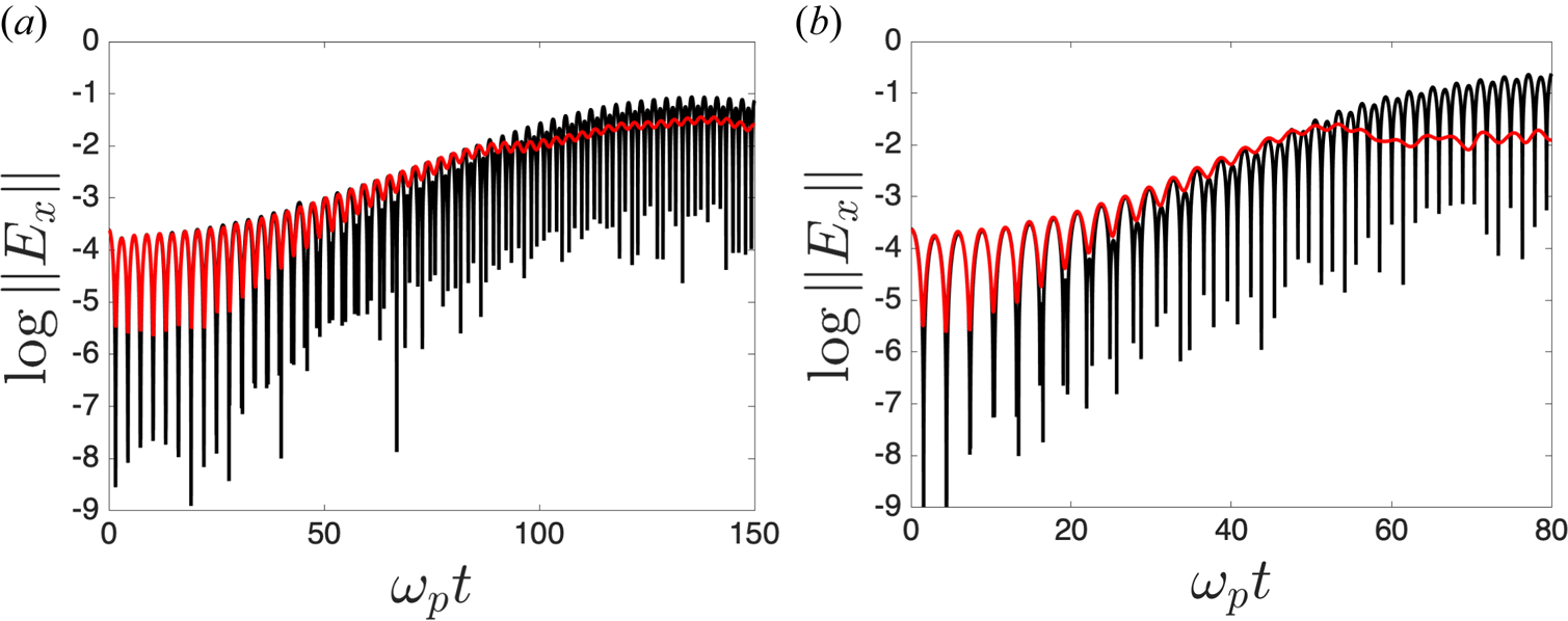
In figure 2, we plot the time evolutions of the longitudinal electric field norm

(5.7)\begin{equation} \| E_x(t)\| = \left(\frac{1}{2}\int _0^L E_x^2 \,\mathrm{d} x \right)^{1/2} \end{equation}

(on a semi-$\log _e$ scale) for two values of the incident wave amplitude ($E_0=0.325$ and $E_0=0.65$). The initial conditions are the same for both codes, but the PIC code displays a higher level of initial fluctuations (noise) that is inherent to the numerical method. This is also why we had to take a somewhat high initial perturbation ($\alpha =0.02$), so that it is significantly larger than the noise level. We can observe a relatively good agreement between these two numerical methods in the linear phase. The observed growth rate ($\gamma \approx 0.03$ for $E_0=0.325$ and $\gamma \approx 0.06$ for $E_0=0.65$) is proportional to the amplitude $E_0$ and close to the value expected from the linear theory ($\gamma \approx 0.04$, see Ghizzo et al. Reference Ghizzo, Bertrand, Shoucri, Johnston, Fijalkow and Feix1990).

Figure 2.

SRS simulations without spin. Time evolution of the amplitude of the longitudinal electric field norm $\|E_x(t)\|$ on a semi-$\log _e$ scale. We compare the results of the Eulerian grid code (black curves) and the PIC code (red curves) for two values of the initial amplitude of the electromagnetic wave. We investigate (a) $E_0=E_\textrm {ref}=0.325$ (observed slope in the linear regime: $\gamma \approx 0.03$) and (b) $E_0=2E_\textrm {ref}=0.65$ ($\gamma \approx 0.06$).

5.2 Spin-dependent model without wave self-consistency

In this part, we study the propagation of a circularly polarized wave into a plasma which does not retroact on the wave. Hence, the electromagnetic wave propagates as if it was in a vacuum. In this case, there is no SRS instability.

With the notations of § 2.2, the model we consider here reads as

(5.8)\begin{equation} \dot{\mathcal{Z}} = \{\mathcal{Z}, \tilde{\mathcal{H}} \}, \end{equation}

where $\mathcal {Z} = (\,f, E_x, E_y, E_z, A_y, A_z)$, $\{{\cdot }, {\cdot } \}$ is the bracket defined in (2.13) and $\tilde {\mathcal {H}}$ is the Hamiltonian defined as

(5.9)\begin{align} \tilde{\mathcal{H}}(\,f, {\boldsymbol E}, {\boldsymbol A}_\perp) &= \frac{1}{2}\int_{\mathbb{R}^5} p^2 f \,\mathrm{d} x\,\mathrm{d}p\,\mathrm{d}{\boldsymbol s} + \frac{1}{2}\int_{\mathbb{R}}\left( |{\boldsymbol E}|^2 + \left|\frac{\partial {\boldsymbol A}_\perp}{\partial x}\right|^2 \right)\,\mathrm{d} x\nonumber\\ &\quad + {\mathfrak{h}} \int_{\mathbb{R}^5} \left( s_y \frac{\partial A_z}{\partial x} - s_z \frac{\partial A_y}{\partial x} \right) f \,\mathrm{d} x\,\mathrm{d}p\,\mathrm{d}{\boldsymbol s}, \end{align}

which means that the term ${\boldsymbol A}_\perp \boldsymbol {\cdot } {\partial {\boldsymbol A}_\perp }/{\partial x} {\partial f}/{\partial p}$ disappears from the Vlasov equation in (2.12), and the terms $A_y \int _{\mathbb {R}^4} f \,\mathrm {d}p\,\mathrm {d}{\boldsymbol s}$, $A_z \int _{\mathbb {R}^4} f \,\mathrm {d}p\,\mathrm {d}{\boldsymbol s}$ disappear from the Maxwell equations in (2.12). In this case, the electromagnetic wave is not coupled to the plasma and can be determined exactly by solving the corresponding Maxwell equations for $E_y$ and $E_z$. In contrast, the longitudinal nonlinearity is kept in the model, hence $E_x$ is a solution of Poisson's equation. The resulting reduced system preserves the geometric structure of the full system.

The initial condition on the distribution function is as follows (see Appendix D):

(5.10)\begin{align} &f(t=0, x, p, \boldsymbol{s}) = \frac{1}{4{\rm \pi}} (1 + \eta s_z) (1+\alpha\cos(k_e x)) \frac{\exp\left({-\dfrac{p^2}{2v_{\textrm{th}}^2}}\right)}{\sqrt{2{\rm \pi}} v_{\textrm{th}}},\notag\\ & \qquad x\in \left[0, \frac{4{\rm \pi}}{k_e}\right], p\in \mathbb{R}, {\boldsymbol{s}\in\mathbb{S}^2}, \end{align}

i.e. it is the product of the initial spin-less distribution function (5.2) times a spin-dependent part. Hence, the spin variables are initially uncorrelated with the positions and velocities of the particles. The spin-dependent part should be fully quantum mechanical, and is therefore obtained from the $2 \times 2$ density matrix for spin-1/2 fermions, with the additional assumption that the spin must be directed either parallel or antiparallel to the $z$ axis (Manfredi et al. Reference Manfredi, Hervieux and Hurst2019) (collinear approximation). More details are given in Appendix D. The variable $\eta$ represents the degree of polarization of the electron gas: $\eta =0$ for an unpolarized gas and $\eta =1$ for a fully polarized gas. Here, we use $\eta =0.5$ and ${\mathfrak{h}}=0.00022$. This value of the scaled Planck constant corresponds to a dense electron gas of density $n_0=10^{31} \ \textrm {m}^{-3}$ and temperature $k_B T = 100 \ \textrm {eV}$. All other parameters take the same values as in the spin-less case treated in § 5.1.

Neglecting the spatial dependence of the magnetic fields, an approximate closed equation for the dynamics of the macroscopic spin ${\boldsymbol S}(t) = \int \boldsymbol {s} f \,\mathrm {d} x \,\mathrm {d}p \,\mathrm {d}\boldsymbol {s}\in \mathbb {R}^3$ can be obtained by integrating the Vlasov equation (2.12) in $(x,p,\boldsymbol {s})$. We get the following ODE system:

(5.11)\begin{equation} \dot{\boldsymbol S} = {\boldsymbol S} \times \boldsymbol{B}, \end{equation}

with $\boldsymbol {B} = (0, -\partial _x A_z, \partial _x A_y)^\mathrm {T}$. Considering a circularly polarized electromagnetic wave, the magnetic field is (still neglecting spatial effects) $\boldsymbol {B}(t) = (0, B_0 \sin (\omega _0 t), -B_0 \sin (\omega _0 t)$, with $B_0=E_0 k_0/\omega _0$. In the regime $B_0/\omega _0 \ll 1$ (i.e. when the Larmor precession frequency $eB_0/m$ is much smaller than the laser frequency), it can be shown that the spin ${ S_z(t)}$ oscillates with a frequency $\omega _\textrm {spin}=B_0^2/(2\omega _0)$ (see Appendix C for details).

Here, this solution will be compared with the evolution of ${\boldsymbol S}(t)$ obtained from the numerical solution of the spin Vlasov–Maxwell equations. As the retroaction terms were removed from the Vlasov equation, there is no SRS instability. Then, the magnetic field of the incident wave remains approximately constant in amplitude, thus justifying the use of (5.11) as a valid approximation.

We use the same physical parameters as in § 5.1 and define the reference magnetic field of the incident wave as

(5.12)\begin{equation} B_\textrm{ref}=\frac{E_\textrm{ref} k_0}{\omega_0} = 0.123 k_0, \quad \text{so that } \quad \frac{B_\textrm{ref}^2}{2\omega_0} = 0.017. \end{equation}

We have that $B_\textrm {ref}/\omega _0 = 0.123 k_0/\omega _0 \approx 0.11$. We will use values up to $B_0=2B_\textrm {ref}$ so that the condition $B_{0}/\omega _0 \ll 1$ is always satisfied, albeit marginally.

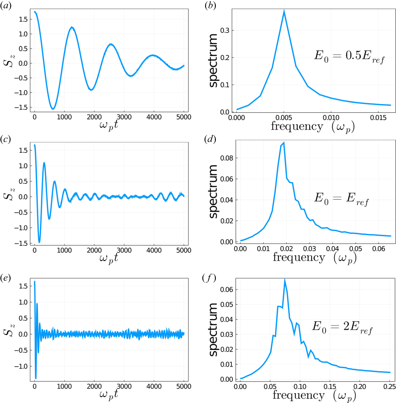
In figure 3, we plot the time evolution of the $z$ component of the macroscopic spin vector $S_z(t) = \int s_z f \,\mathrm {d} x \,\mathrm {d}p \,\mathrm {d}\boldsymbol {s}$ and its frequency spectrum (the frequencies are expressed in units of $2{\rm \pi} /T$, where $T$ is the final simulation time) for three different values of $E_0$ (and hence $B_0$): $E_0 =0.5E_\textrm {ref}$, $E_0 =E_\textrm {ref}$ and $E_0 =2E_\textrm {ref}$. Here, ${ {S}}_z$ displays a damped oscillatory behaviour with a spectrum that is well-localized around a single frequency. This dominant frequency is close to the theoretical value $\omega _\textrm {spin}=B_0^2/(2\omega _0)$, which yields $\omega _\textrm {spin}=0.0043, \, 0.018$ and $0.068$ for the three cases considered here. In particular, the quadratic scaling between $\omega _\textrm {spin}$ and $B_0$ is well respected.

Figure 3.

Spin-dependent model without wave self-consistency for three values of the incident wave amplitude: $E_0 =0.5E_\textrm {ref}$ (a,b), $E_0 =E_\textrm {ref}$ (c,d) and $E_0 =2E_\textrm {ref}$ (e, f). (a,c,e) Time history of ${ {S}}_z(t)$ (time is in units of $\omega _p^{-1}$). (b,d, f) Corresponding frequency spectrum in units of $\omega _p$. The expected values of the spin precession frequencies are (from a,b to e, f) $\omega _\textrm {spin}=0.0043, \, 0.018$ and $0.068$.

The observed damping is likely to arise from phase mixing in the phase space and its rate also increases rapidly with $E_0$. The effect of the temperature on the damping will be studied in more details in the next subsection.

5.3 Full spin-dependent model

In this section, we consider the full spin Vlasov–Maxwell model (2.12) and study the influence of several physical parameters on the spin dynamics. In particular, we will analyse the effect of the incident wave amplitude, the electronic temperature, the initial spin polarization and the scaled Planck constant. The remaining physical parameters are those of § 5.1.

We will consider two types of initial conditions for the distribution function. The first (labelled ‘Wigner’) is the one already used in the preceding subsection, see (5.10), and corresponds to a quantum density matrix for an ensemble of spins directed parallel to the $z$ axis. The second initial condition (labelled ‘Dirac’) corresponds to an ensemble of classical spins all having directions along the $z$ axis; it does not correspond to any quantum state and is used here only to illustrate more clearly the loss of spin polarization in the electron gas.

5.3.1 Wigner initial condition

The initial condition is the Maxwell–Boltzmann distribution of (5.10), whose derivation is detailed in Appendix D. The physical parameters are the same as in our reference case described in § 5.1. The electromagnetic fields are initialized as in (5.3). The numerical parameters are as follows: $\Delta t=0.04, N_p=2\times 10^4, N_x=128$.

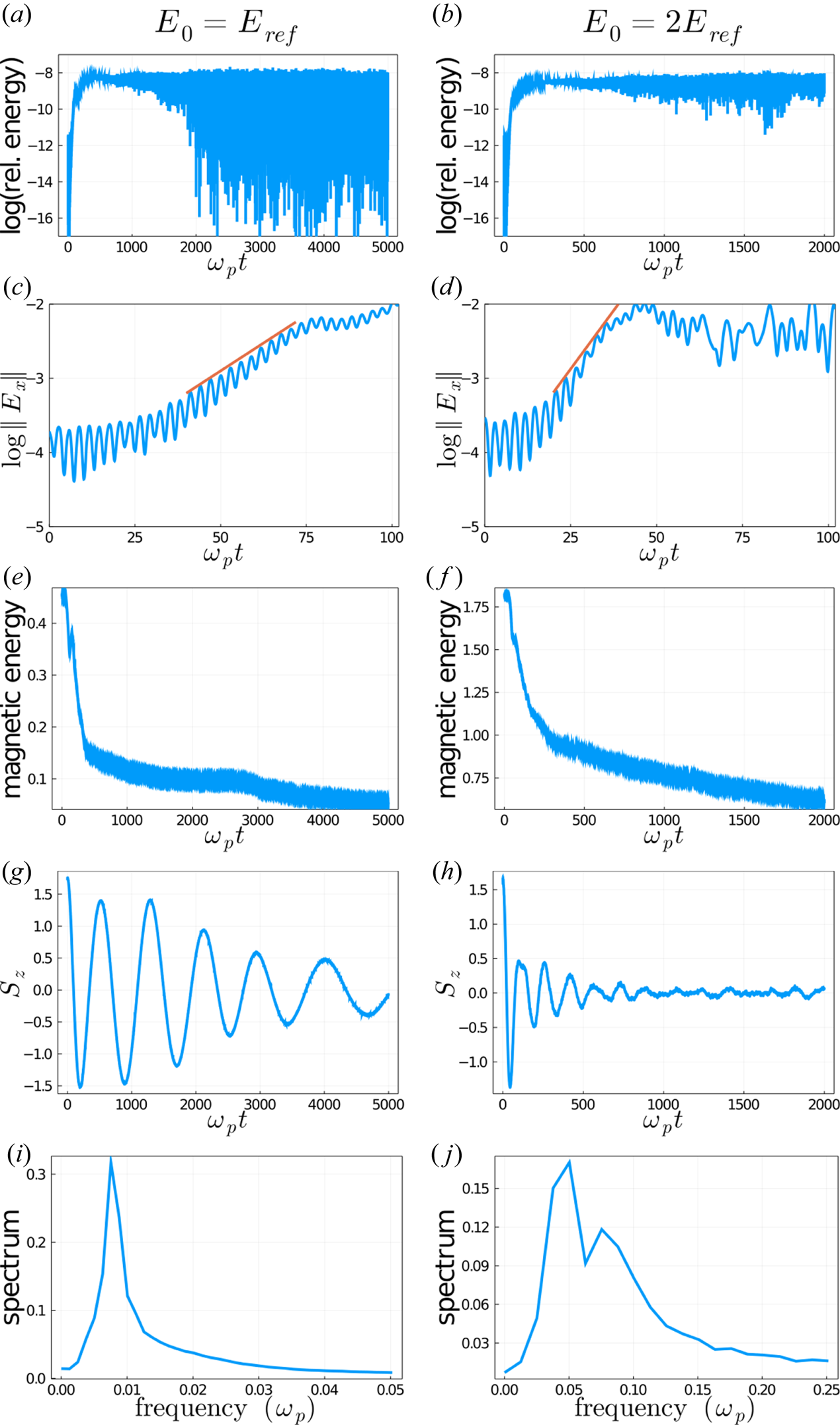
Laser field amplitude. In figure 4, we study the influence of the incident wave amplitude $E_0$, using ${\mathfrak{h}}=0.00022$. The two columns in the figure refer to two values of $E_0$: $E_\textrm {ref}$ on the left and $2E_\textrm {ref}$ on the right. Conservation of the total energy is good for the PIC code standards, with an error on the relative energy $|{\mathcal {E}}_\textrm {tot} (t)-{\mathcal {E}}_\textrm {tot} (0)|/{\mathcal {E}}_\textrm {tot} (0)$ of approximately $3\times 10^{-4}$. This good conservation property arises from the fact that our algorithm is a fully discrete structure-preserving method.

Figure 4.

Full spin-dependent model. We illustrate the influence of the amplitude $E_0$ of the incident wave for (a,c,e,g,i) $E_0=E_\textrm {ref}$ and (b,d, f,h,j) $E_0= 2E_\textrm {ref}$. (a,b) Time history of the the relative total energy $|{\mathcal {E}}_\textrm {tot} (t)-{\mathcal {E}}_\textrm {tot} (0)|/{\mathcal {E}}_\textrm {tot} (0)$ (on a semi-$\log _e$ scale). (c,d) Time history of the longitudinal electric field norm $\|E_x\|$ (on a semi-$\log _e$ scale); the red straight lines have slopes 0.03 (c) and 0.06 (d). (e, f) Magnetic energy $({1}/{2}) \int |B|^2 {\textrm {d} x}$. (g,h) Time history of the spin component ${ {{S}}}_z(t)$. (i, j) Frequency spectrum of ${ {{S}}}_z$.

The instability rate, measured from the growth of the longitudinal electric field amplitude $\|E_x(t)\|$, is very similar to that observed in the spin-less simulations, namely $\gamma =0.03$ ($E_0=E_\textrm {ref}$) and $\gamma =0.06$ ($E_0=2E_\textrm {ref}$).

The instability has a strong impact on the spin dynamics. In particular, the $z$ component of the macroscopic spin ${ {S}}_z(t) = \int s_z f \,\mathrm {d} x \,\mathrm {d}p \,\mathrm {d}\boldsymbol {s}$ is damped much more efficiently in the large-amplitude case (right column), where the instability develops faster and saturates at a higher level. The frequency spectrum of ${ {S}}_z(t)$ displays in both cases a well-defined peak. There is a factor of approximately 5.5 between the spin precession frequencies observed for $E_0=E_\textrm {ref}$ and $E_0=2E_\textrm {ref}$. This is slightly larger that the quadratic scaling with $E_0$ predicted by our simple model $\omega _\textrm {spin}=B_0^2/(2\omega _0)$ (see § 5.2 and Appendix C for further details). However, one must recall that this expression was derived under the assumption of an incident wave of constant amplitude $E_0$. Here, in contrast, the amplitude is modulated in time, which then affects the quadratic scaling.

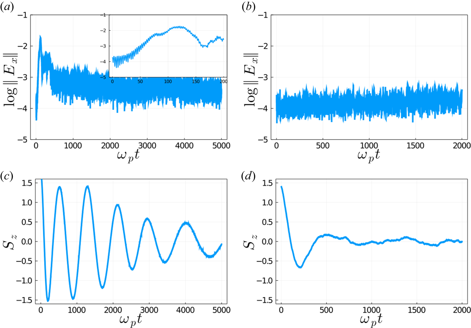
Thermal effects. Next, we study the influence of the temperature by considering two values of the thermal speed: $v_{\textrm {th}}=0.17$ (as in the previous results of figure 3) and $v_{\textrm {th}}=0.51$, while the field amplitude is fixed to $E_0=E_\textrm {ref}$ and ${\mathfrak{h}}=0.00022$. The wave number $k_e$ also changes, as it is dependent on the temperature ($k_e=1.22$ and $k_e=1.46$, for the low-temperature and high-temperature cases, respectively), but the matching conditions of (5.4a,b) are still satisfied with $k_0=2k_e$ and $\omega _0^2=1+k_0^2$.

The simulation results are shown in figure 5. In the high-temperature case, the instability is clearly suppressed, nevertheless, the spin is damped much faster than in the ‘cold’ case. Furthermore, we checked that when no laser pulse is present at all (i.e. $E_0 = 0$, not shown here), no loss of the polarization is observed.

Figure 5.

Full spin-dependent model. Influence of the electron temperature using two values of the thermal speed: $v_{\textrm {th}}=0.17$ (a,c) and $v_{\textrm {th}}=0.51$ (b,d). For both cases, the field amplitude is $E_0=E_\textrm {ref}$. Here, (a,b) show the time history of the longitudinal electric field norm (on a semi-$\log _e$ scale) and (c,d) show the time history of the spin component ${ {{S}}}_z(t)$. The inset in (a) displays a zoom of the longitudinal electric field evolution in the time range $\omega _p t \in [0, 200]$, which shows the development of the linear instability.

This is an intriguing result. First, it reveals that the laser pulse is mandatory to induce some loss of polarization. When the laser wave amplitude $E_0$ is sufficiently high and the plasma is sufficiently cold, the SRS instability is triggered, and this induces a loss of spin polarization in the electron gas. This loss of polarization is faster for larger wave amplitudes (figure 4). For warmer plasmas, the SRS instability is suppressed, but depolarization still occurs owing to temperature effects (figure 5). Nevertheless, the presence of the electromagnetic wave is still necessary to observe this ‘thermal’ loss of polarization.

Such depolarization mechanisms are akin to the ultrafast demagnetization observed in metallic nanostructures irradiated with femtosecond laser pulses (Beaurepaire et al. Reference Beaurepaire, Merle, Daunois and Bigot1996; Bigot et al. Reference Bigot, Vomir and Beaurepaire2009; Bigot & Vomir Reference Bigot and Vomir2013).

Scaled Planck constant and initial polarization. In figure 6, the time history of $S_z(t)$ is displayed for $\eta =0.5$ and different values of the scaled Planck constant: ${\mathfrak{h}}=0.00022, 0.05, 0.1$ and 0.2. The influence of ${\mathfrak{h}}$ on the spin dynamics is rather modest and becomes appreciable only for values that are approaching unity. The main observable effect is an increase of the oscillation period with the scaled Planck constant.

Figure 6.

Full spin-dependent model. Influence of ${\mathfrak{h}}$ on ${ {{S}}}_z(t)$: (a) ${\mathfrak{h}}=0.00022$; (b) ${\mathfrak{h}}=0.05$; (c) ${\mathfrak{h}}=0.1$; (d) ${\mathfrak{h}}=0.2$. For all cases, the initial spin polarization is $\eta =0.5$.

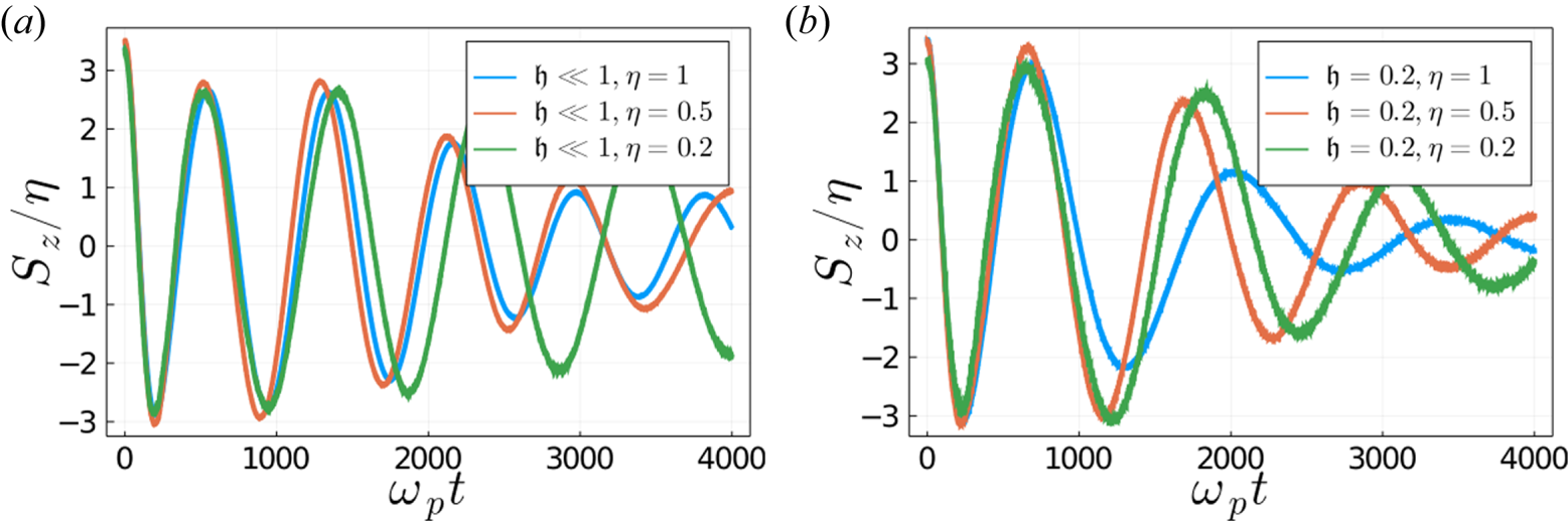
Figure 7 shows the influence of the initial electron polarization ($\eta =0.2, 0.5$ and 1) for two different values of the scaled Planck constant, ${\mathfrak{h}}=0.00022$ and ${\mathfrak{h}}=0.2$. The initial value of the macroscopic spin ${ {{S}}}_z$ is given by ${ {{S}}}_z(t=0)=L\langle s_z \rangle =L\eta /3\approx 3.42\eta$, see also Appendix D. Hence, to compare results with different values of $\eta$, we plot the quantity ${ {{S}}}_z(t)/\eta$. At low ${\mathfrak{h}}$, the effect of $\eta$ is weak. In contrast, for large ${\mathfrak{h}}$, a larger initial polarization is associated with a stronger damping of the macroscopic spin.

Figure 7.

Full spin dependent model. Influence of the initial polarization $\eta$ for two values of the scaled Planck constant ${\mathfrak{h}}$. We plot the ratio ${ {{S}}}_z(t)/\eta$, which is initially independent of $\eta$, for (a) ${\mathfrak{h}}=0.00022, \eta =0.2, 0.5,\ \textrm {and}\ 1$; (b) ${\mathfrak{h}}=0.2, \eta =0.2, 0.5, \ \textrm {and} \ 1$.

Spin dynamics. To investigate the microscopic spin dynamics in more detail, we have divided the interval of values taken by the spin component $s_z \in [-1,+1]$ into 200 bins each with a size of 0.01. We call $N(s_z)$ the number of particles having the spin component $s_z$ in an interval around $s_z$, and $N_p$ is the total number of particles. In figure 8(a–k), we show the histograms of $N(s_z)/N_p$ as a function of $s_z$ at different times. The electron distribution at $t=0$ is linear in $s_z$, as shown in (5.10) and in Appendix D. In this case, the electron gas is initially fully polarized along the positive $z$ direction so that the distribution goes from $N(s_z)/N_p=0$ for $s_z=-1$ to $N(s_z)/N_p=1$ for $s_z=1$.

Figure 8.

Full spin-dependent model. Histograms of $s_z$ at different times, for a case with ${\mathfrak{h}}=0.00022, v_{\textrm {th}}=0.17, \eta =1$. From (a–k): $\omega _p t=0, 100, 200, 300, 400, 500, 600, 1000, 1500, 3000$ and 4000. Here, $N(s_z)$ is the number of particles having the $z$ spin component in an interval around $s_z$ and $N_p$ is the total number of particles. The frame (l) shows the time history of the global spin component ${ {{S}}}_z(t)$. The red dots correspond to the times of the different histograms displayed in (a–k).

For instance, one can see that at $\omega _p t=200$ (figure 8c), the spin direction has completely reversed, which indicates that the global spin now points along the negative $z$ direction. In contrast, at $\omega _p t=1500$ (figure 8i), the distribution is flat, which indicates that the global spin is close to zero. The slope of the spin distribution decreases progressively with time, thus revealing some amount of damping. This behaviour is confirmed by the time history of the global spin component ${ {{S}}}_z(t)$, shown in figure 8(l).

5.3.2 Dirac initial condition

We consider the following initial condition for the distribution function:

(5.13)\begin{gather} f_0(x,p,\boldsymbol{s}) = (1+\alpha\cos(k_ex)) \frac{1}{\sqrt{2{\rm \pi}} v_{\textrm{th}}} \exp\left({-\frac{p^2}{2v_{\textrm{th}}^2}}\right) \delta(\boldsymbol{s}-(0, 0, 1)^\mathrm{T}), \nonumber\\ x \in \left[0,\frac{4{\rm \pi}}{k_e}\right], \ p \in \mathbb{R}, \boldsymbol{s}\in\mathbb{S}^2, \end{gather}

which corresponds to an ensemble of classical spins which are all directed along the positive $z$ axis. This distribution does not have a clear quantum mechanical meaning, as it does not correspond to any actual Wigner function or density matrix. However, it is useful to perform some numerical simulations with this initial condition, as it enables us to better highlight the dynamics of the spin of the particles on the unit sphere.

The parameters of the electromagnetic fields are the same as those in § 5.1, with $E_0=E_\textrm {ref}$ and ${\mathfrak{h}}=0.00022$. In figures 9 and 10, we show the spins $\boldsymbol {s}$ of the electrons at different instants $t$, together with the time history of the global spin components ${ {{S}}}_y(t)$ and ${ {{S}}}_z(t)$, for two values of the thermal speed $v_{\textrm {th}}=0.17$ (figure 9) and $v_{\textrm {th}}=0.51$ (figure 10). At $t=0$, the spin variables of all particles are localized at the north pole of the sphere, as indicated by the single red dot in the initial condition.

Figure 9.

Full spin-dependent model with Dirac initial condition and $v_{\textrm {th}}=0.17$. Panels (a–i): distribution of the spins on the unit sphere at times $\omega _p t=0, 100, 200, 300, 400, 500, 600, 1000$ and 1500. Panels ( j,k) show the time history of ${ {{S}}}_y(t)$ and ${ {{S}}}_z(t)$, the red dots correspond to the times of the different snapshots displayed in (a–i).

Figure 10.

Full spin-dependent model with Dirac initial condition and $v_{\textrm {th}}=0.51$. Panels (a–i): distribution of the spins on the unit sphere, at times $\omega _p t=0, 100, 200, 300, 400, 500, 600, 1000$, and 1500. Panels ( j,k) show the time history of ${ {{S}}}_y(t)$ and ${ {{S}}}_z(t)$, the red dots correspond to the times of the different snapshots displayed in (a–i).

First, we remark that the spin vector of each particle remains on the unit sphere: $|\boldsymbol {s}_a(t)|=1, \forall a=1, \ldots , N_p$ and $\forall t>0$. This is of course the case for the continuous model, but it is worth emphasizing that our numerical scheme is capable of capturing this important geometric property exactly.

At later times, the spin distribution broadens and explores most of the surface of the sphere. For $v_{\textrm {th}}=0.17$, the distribution moves around the surface of the sphere but remains rather localized on it. This is in line with the evolution of the global spin components ${{{S}}}_{y,z}(t)$ (figure 9j–k), which oscillate with little damping. For $v_{\textrm {th}}=0.51$, the distribution covers the surface of the sphere more uniformly, although the motion is not completely ergodic, and some ring-shaped structures are still visible at times $\omega _p t \gtrsim 1000$. This is also consistent with the corresponding evolution of the spin components $S_{y,z}(t)$ (figure 10j–k), which are more heavily damped than in the low-temperature case.