


1. Introduction
Recent efforts to indirectly generate Arctic and Antarctic sea-ice thickness profiles utilizing Geoscience Laser Altimeter System (GLAS)/Ice, Cloud and land Elevation Satellite (ICESat) laser altimetric assessments of sea-ice freeboard height and isostatic buoyancy principles have demonstrated a promising methodology for regional-scale sea-ice thickness characterization (Reference Spreen, Kern, Forsberg and HaarpaintnerSpreen and others, 2006; Reference Kwok, Cunningham, Zwally and YiKwok and others, 2007; Reference Zwally, Yi, Kwok and ZhaoZwally and others, 2008). Assessments of sea-ice thickness that have relied upon upward-looking-sonar (Reference Strass, Tian and NemotoStrass and others, 1998; Reference Renner and LytleRenner and Lytle, 2007) and actual drilling (Reference Wadhams, Lange and AckleyWadhams and others, 1987; Reference Lange and EickenLange and Eicken, 1991; Reference Haas, Nicolaus, Worby and FlinspachHaas and others, 2008), though offering the greatest probability of accuracy, are severely limited by their spatial and temporal scale and coverage. the derivation of ice thickness estimations through Antarctic Sea Ice Processes and Climate (ASPeCt) observational methods (Reference Worby and DiritaWorby and Dirita, 1999; Reference Worby, Allison and DiritaWorby and others, 1999, Reference Worby, Geiger, Paget, Ackley and DeLiberty2008) as well as through electromagnetic induction (EMI) methods (Reference Kovacs, Valleau and HolladayKovacs and others, 1987; Reference HaasHaas, 1998; Reference Reid, Worby, Vrbancich and MunroReid and others, 2003, Reference Reid, Pfaffling, Worby and Bishop2006) address in part the spatio-temporal coverage issues, but are potentially limited by observational and sampling bias inherent in the ASPeCt technique and by technical constraints as well as sampling bias for the EMI technique.
The derivation of ice thickness by altimetry/buoyancy methods is not without its challenges, however. Snow depth information is crucial to the application of buoyancy principles for derivation of ice thickness, as the difference of snow depth and elevation (snow surface freeboard) allows for the determination of the snow–ice interface (ice free-board). Efforts to derive snow depths on a regional scale have been based on a combination of microwave radar altimetry and laser altimetry (Conner and others, 2009), passive microwave from the Advanced Microwave Scanning Radiometer– Earth Observing System (AMSR-E; Reference KurtzKurtz and others, 2009), and meteorological-observation/snow-climatology models (Reference WarrenWarren and others, 1999). Snow depth estimation from any of the methods listed above has proven to be problematic. Significant spatial resolution differences in radar vs laser altimeters and radar footprint location are problematic for altimetry methods. Depth limitation, snow grain size, wetness, and presence of slush confounding microwave emissions are problematic for AMSR-E methods. Climatology models are problematic for their over-generalization.
Accurate derivation of the sea-ice freeboard elevation by satellite laser ranging is only as good as the known position of sea surface height (SSH), represented by the mean equipotential sea surface elevation (the marine geoid) filtered to exclude sea surface response to atmospheric pressure loading, tides, currents, etc. In early attempts to derive freeboard from calculated SSH (as the reference level), subsequent uncertainties in the available geoid led to large unrealistic errors in freeboard and thus ice thickness (Reference Forsberg and SkourupForsberg and Skourup, 2005; Reference Kwok, Cunningham, Zwally and YiKwok and others, 2006). Later efforts to determine SSH utilizing direct laser altimeter detection of open water and leads along ICESat transits has significantly improved derivation of freeboards at basin scale (Reference Kwok, Cunningham, Zwally and YiKwok and others, 2007; Reference Zwally, Yi, Kwok and ZhaoZwally and others, 2008; Reference Farrell, Laxon, McAdoo, Yi and ZwallyFarrell and others, 2009). Due to the spatial and temporal availability of leads for a SSH reference, both Reference Zwally, Yi, Kwok and ZhaoZwally and others (2008) and Reference Farrell, Laxon, McAdoo, Yi and ZwallyFarrell and others (2009) developed an ICESat transit sampling range in the order of 25–50km for the derivation of freeboard. Reference KurtzKurtz and others (2009) also utilized a sampling scale on the order of 12.5–25km based in part on the gridcell size of AMSR-E for snow depth estimation and in part on the ICESat freeboard retrieval length scale. These length scales, resulting from the most recent and successful efforts to derive altimetric ice thickness distributions for both Arctic and Antarctic sea ice, have significant implications for the question to be addressed in this study. That is, within this 12.5–50km retrieval range of ICESat, can altimeter-based sea-ice elevation estimations, at the laser spot size of ~70m and interval of ~170 m, realistically yield a derived sea-ice thickness mean and distribution consistent with in situ observed ice type heterogeneity, given inherent spatial averaging? Through a modeling simulation of an ICESat altimetric estimation of sea-ice elevation, parameterized by in situ data collected in the Bellingshausen Sea, Antarctica, in 2007, we derive the minimum number of altimeter elevation samples to statistically recreate the in situ mean ice thickness and distribution utilizing isostatic buoyancy principles and assumptions of ice freeboard.
2. Background
A comprehensive in situ geophysical characterization of sea ice at Ice Station Belgica (ISB) in the Bellingshausen Sea, during the 2007 Sea Ice Mass Balance in Antarctica (SIMBA) expedition, yielded a robust set of spatial and temporal measurements of sea-ice elevation (snow surface), snow depth, ice freeboard elevation and ice thickness on a 5 km2 floe comprising mixed first- and multi-year ice (Reference LewisLewis and others, in press; Reference Weissling, Lewis and AckleyWeissling and others, in press). the initial ASPeCt observations of ISB ice type were 60% first-year and 40% multi-year, with snow depths of 25–40 and 75–100cm on first- and multi-year ice respectively. Ice thickness estimated from ASPeCt visual assessment of the overturned ice blocks (during initial ship approach to ISB) was >1.2m for level first-year and 2 m for level multi-year, or only two types. Subsequent in situ ice assessment based on surface elevation surveys, ruler-stick snow depth surveys, drilling, and EMI ice thickness surveys, combined with photo-visual documentation of the floe and GPS mapping, provided strong evidence that the ISB floe was composed of not two but three spatially and physically discrete ice regimes. Characterization of the three ice regimes (herein referred to as ice towns) was based on the three primary geophysical study sites, named Fabra (FAB), Patria/Lie`ge (PAL) and Brussels (BRU).
The FAB, PAL and BRU ice types were visually assessed during the drift experiment to represent a sizable fraction of the floe’s total area, approximately 40%, 40% and 20% respectively, with FAB ice being predominately multi-year and PAL/BRU ice being first-year ice. This 40%/60% split is consistent with the ASPeCt ice type observation during the inbound transit. Post-cruise evaluation of satellite radar (RADARSAT and Envisat) and visual spectrum imagery (Moderate Resolution Imaging Spectroradiometer (MODIS)) suggested that the ISB floe, during the drift experiment, was located at a transition line between predominately first-year ice to the north and mixed first- and multi-year ice to the south, with the ISB floe representative of the latter (Fig. 1). Table 1 lists the respective snow and ice parameters of the three ice towns as assessed from the geophysical experiments. Locations of the geophysical experiment sites with respect to a generalized map depiction of the ISB floe, subdivided into the three ice towns, can be seen in Figure 2.
Aqua MODIS image dated 13 October 2007, 20:35 UTC. ISB floe is at center of black circle. Shown clearly in this image is the transition between predominately first-year ice to the north of the large lead and mixed first- and multi-year ice to the south.

Generalized map of the ISB floe depicting geophysical study site locations and ice towns Brussels (lower left), Patria/Liège (upper section) and Fabra (lower right). Percentages of ice town areas are approximate. Photograph was taken from the ship looking northwest across floe toward the open lead. Brussels ice can be visually distinguished from Fabra ice by surface texture.

Summary statistics of in situ sea-ice characteristics of ISB ice towns FAB, PAL and BRU as assessed October 2007

One key element of the ice town parameters that is crucial to the premise and objective of this study is the elevation of the ice freeboard surface (snow/ice interface). As discussed in the introduction, knowledge of snow depth, and thus the elevation of the ice freeboard, from remote sensing is problematic. Temporal series data from the ISB experiment strongly indicated the formation of snow ice in the thicker first- and multi-year ice types from the freezing of slush layers at the snow–ice interface. the net effect from this phenomenon was to maintain a zero-elevation ice freeboard surface. From the perspective of Antarctic late-winter–early-spring, near-maxima ice thickness and extent conditions, our in situ drift station observations indicated that on a floe scale (kilometers) ice freeboard is essentially at sea level (0.0±0.02 m). Post-cruise assessments of our underway observations (EMI ice thickness assessments and three in situ ice stations) as well as analysis of our inbound and outbound ASPeCt observations likewise indicated ice freeboard at or near sea level on a regional scale (tens to hundreds of kilometers). In other words, snow depth is equivalent to snow surface elevation (Reference Weissling, Lewis and AckleyWeissling and others, in press; Reference XieXie and others, in press). This has important implications for satellite-based altimetry methods for deriving ice thickness from buoyancy principles, in that a mean ice freeboard at sea level obviates the need for specific spatial distribution of snow depth, and that ice freeboard can be estimated from snow elevation alone.
3. Methods
The process of analysis for this study was based on a simulation of ICESat altimetry sampling of two modeled ice floes as analogs for the regional ice conditions observed and assessed during the ISB drift station experiment. As mentioned previously, the location of the ISB floe was in a transitional area between mixed first- and multi-year ice to the south of which the ISB floe was considered representative (based on RADARSAT backscatter similarities with its surroundings), and predominately first-year ice to the north. As such, this simulation model considered both situations, with a 40–40–20 fractional coverage representing ice towns FAB, PAL and BRU respectively (model 1), and an 80–20 fractional coverage representing ice towns PAL and BRU respectively (model 2).
The analysis lent itself to a coding environment based on imagery analysis techniques and, as such, was coded in Interactive Data Language (IDL), the language platform for ENVI v4.7, ITT Visual Information Solutions.
3.1. Ice-floe model map
The first step of this study was to create two model floes comprising a spatial generalization of the three ice towns with simulated elevation, snow-depth and ice thickness distributions consistent with the in situ distributions. For ease of coding and subsequent analysis, the ISB floe shape was generalized as a square, 2240m on a side (5.02km2). A nominal analysis dimension of 10 m (pixel dimension) was chosen to be consistent with the scale of the ICESat sampling interval of ~170m and laser spot-size diameter of ~70 m. A 10m analysis dimension was also consistent with the dimensional scale of deformed sea ice being in isostatic equilibrium as evaluated by Reference Weissling, Lewis and AckleyWeissling and others (in press).
To mimic the sea-ice heterogeneity within each of the simulated ice towns of the resultant 224×224 pixel floe images, each pixel was randomly assigned a value of elevation and snow depth constrained by the known (in situ) probability distributions for each ice type. the identical random number sequence was used to generate both elevation and snow depths for a given pixel to force some linearity in the elevation–snow-depth relation (i.e. greater elevation likely implies greater snow depth). Example images of the simulated floe-map images for models 1 and 2 and an elevation profile across model 1 are shown in Figure 3.
Depictions of model 1 and model 2 simulated floes with designated ice towns BRU, PAL and FAB. Cross section A–A' across model 1 shows respective elevations and elevation variability within each town. Texture pattern of each ice town is symbolic of relative variance of elevation. Dark tones indicate thinner ice; light tones thicker ice.

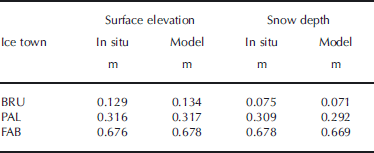
Each image is actually a composite three-band raster, with band 1 containing a numerical descriptor for the ice type, band 2 containing the elevation information and band 3 containing the snow depth information. Although the snow depth information of these floe images is not needed for the final altimetry sampling simulation, it was specifically generated to assess the model accuracy of the simulated vs measured means and variance of ice town elevation and snow depths. As can be seen in Table 2, the modeled and in situ data agree exceptionally well, as expected given the validity of the model construction.
Comparison of in situ and modeled surface elevation and snow depth of ISB ice towns
3.2. Altimeter track and sampling model
Although ICESat altimeter passes transect the region of the Bellingshausen Sea in slightly converging north–south orientations depending on ascending or descending orbits, translation and rotation of the pack ice over time results in the possibility of randomly oriented transects over a given area. Therefore, modeling multiple randomly placed altimeter passes over the floe maps serves as a proxy for a single, continuous transit of the regional sea ice, with a repeated but randomly ordered sampling of the three ice towns and their corresponding elevation distributions.
IDL code was written to generate a random starting point along any one of the four sides of the floe map, followed by a randomly generated azimuth, the net effect being to generate a single pass across the floe. Given an altimeter sampling spacing of 170 m, a single pass could result in as few as one hit (on a map corner) or as many as 19 hits (along the map diagonal). Therefore, any one altimeter pass over the simulated floe map would have a very low probability of sampling all three ice towns in the same fractional percentage, and thus a low probability of generating an elevation mean and distribution statistically equivalent to the floe itself. Additional passes (and thus an increasing number of sampling hits) would have the ultimate effect of a more uniform spatial sampling of the floe. Figure 4 depicts the sampling distribution of the floe after one set of 100 altimeter passes. the black border demarcates the floe boundary. Hits that occurred just outside the floe boundary are a result of the coding structure and were not included in the final sampling of floe elevation.
Example map of simulated ICESat altimeter sampling locations for 100 randomly oriented tracks over the model 1 floe. Scales are in pixels (1 pixel = 10 m).

As can be seen in Figure 4, there is certainly some non-uniformity in the spatial distribution of hits. Statistically, this is to be expected, as each set of 100 pass hits represents a sampling distribution of the population. Designing the model to include replication of sampling therefore provides for an appropriate calculation of the mean and variance of model variables.
The modeling code generated 25 replicates of 100 randomly located altimeter passes across the model 1 and model 2 floe maps. For the ensuing discussion, each set of 100 passes will be referred to as a single altimeter transit. the mean number of sampling hits of the floe for each transit was approximately 900. This mean equates to a continuous altimeter pass of ~153 km, which is consistent with regionally observed ICESat transits acquired in clear sky conditions during the October–November 2007 time frame of the ISB drift station.
3.3. Buoyancy and ice thickness modeling
The assumption of an ice freeboard at or about sea level (0.0 m) significantly facilitates the derivation of ice thickness by buoyancy principles, leaving the primary variable in the equation that of surface elevation. the ICESat laser spot at the surface has been estimated to be ~70m diameter or ~3850m2. the closest approximation to that dimension for the simulation model, given a 10 m pixel dimension and the need for symmetry (for ease of coding), was a 7×7 pixel array with 3 pixels removed from each corner, leaving a symmetrical 37-pixel (3700m2) sampling array. For each altimeter laser sampling location or ‘hit’ along the simulated tracks across the model floes, the sampling array would extract the values of 37 individual pixel elevation values centered on the hit location and subsequently calculate the mean elevation for each hit. This elevation value was then entered into the buoyancy Equations (1) and (2) for the derivation of mean ice thickness for each sampling hit.


where ρ s, ρ i, ρ sl and ρ w are bulk densities of snow (320 kgm–3), ice (917 kgm–3), slush (940 kgm–3) and sea water (1027 kgm–3) respectively, and h f, h s and h i are ice freeboard (m), snow (m) and ice thicknesses (m) respectively.
4. Results and Discussion
For model 1, ice towns BRU, PAL and FAB had elevations of 0.134 ±0.040 m (mean ± 1 standard deviation), 0.317±0.062m and 0.678±0.293 m, respectively. Using the constituent densities listed above for snow, ice and sea water, these elevations corresponded to buoyancy-derived ice thicknesses of 0.390, 0.922 and 1.972 m. For model 2, mean elevations and derived ice thickness of the two ice towns PAL and BRU did not change as was expected, although a new random simulation of the floe map was produced. In consideration of the fractional distribution of each ice town, model 1 produced a composite elevation of 0.425 ±0.289 m and a mean derived ice thickness of 1.236 m. Model 2 produced a composite elevation of 0.289±0.089m and a mean derived ice thickness of 0.840 m.
For both models, 25 transit replicates over the floe were generated in the simulation, with a sample spacing of 170 m. As mentioned previously, each transit yielded ~900 altimeter hits of the simulated floe snow surface that were subsequently converted to ice thickness. As was expected, each transit’s running mean or cumulative average (Equation (3)) of ice thickness for successive altimeter hits approached the overall mean ice thickness of the floe, with some expected variability in the transit replicates. Figure 5 shows the running mean ice thickness as a function of successive hits forthe first ten transit replicates of model 1.
Graph of ten ICESat transit replicates of the running mean (cumulative average) ice thicknesses for model 1.


where h is ice thickness and j is the sequence of values (i.e. the fifth running mean is the average of the first five hits).
The question to be answered here then becomes at what point does the running transit mean sufficiently describe the known floe mean with an acceptable degree of variance, or, in other words, what is the convergence point? We approached this problem by generating the mean and standard deviation (SD) of all 25 replicates of the transit running means of ice thickness on a hit-by-hit basis. These replicate means should also converge asymptotically to the floe mean with successive hits, while the SD should converge asymptotically to zero. A second method we devised for selecting a simulation stop point was based on the number of hits required to spatially sample all three ice towns (for model 1) in the same fractional percentage (e.g. 40–40–20) as the fractional areas of each town. We accomplished this by assigning a number identifier to each ice type: 1 for BRU, 2 for PAL and 3 for FAB. the fractional mean of ice type identifiers for model 1 then becomes 2.20. For the 80%–20% of PAL and BRU ice towns of model 2, the fractional mean becomes 1.85. Plotted in Figure 6 and 7 are the means and SD of all replicates of the transit ice-thickness running means and the transit ice type identifier running means for models 1 and 2, respectively.
Plots of the replicate (n = 25) mean ice thickness and SD of the transit ice thickness running means (a) and the replicate (n = 25) mean ice type identifier and SD of the transit ice type identifier running means (b) for model 1.

Same as Figure 6, but for model 2.

For model 1, the first candidate for a stop point occurs at ~115 hits with an ice type identifier of 2.17±0.12 and with an ice thickness of 1.20±0.10 m. the abrupt change in slope (marked with the solid vertical line in Fig. 6) of the SD plots, in particular, suggests this stop point. the second candidate for a convergence point is at ~240 hits (marked with the dashed vertical line in Fig. 6). Although there is some additional reduction in variance (0.08 vs 0.10 m SD), and thus slight improvement in the model with an additional 120+ hits, there was no significant change in the ice thickness at 1.19 m.
For model 2, the first candidate for a convergence point (solid vertical line) occurs at ~85 hits with an ice type identifier of 1.86±0.04 and with an ice thickness of 0.84±0.02 m. the second candidate for a convergence point is at ~190 hits (dashed vertical line). Likewise for model 2, the additional 100 or so hits do not contribute significantly to model improvement.
The ice thickness frequency distribution derived from the 115 altimeter hits on the model 1 floe compared to the thickness distribution from all hits is depicted in Figure 8. the excellent agreement between the two distributions does suggest that the 115-hit subset is statistically equivalent to the full set (and likewise for the 85-hit subset of model 2). Converted to an ICESat linear transect, the 115 hits of model 1 would be equivalent to 19.5 km of continuous altimeter sampling for mixed first- and multi-year ice types, while the 85 hits of model 2 would be equivalent to 14.5 km of continuous altimeter sampling for first-year-only ice types. the lengths of both of these sampling transits are within the ICESat effective retrieval range of 12.5–50km for accurate determination of sea-ice elevation and as such are validation of the most current efforts to employ satellite-based methods for sea-ice characterization.
Ice thickness probability distributions for BRU, PAL and FAB ice towns for a 115-sample subset compared to all data for 25 replicate transits of the model 1 floe.

Future work on this simulation model will involve analysis of the most optimal sampling subsets considering varying fractional distributions of sea-ice types and freeboard characteristics but, more importantly, the different altimeter spot (or sampling) size and spot spacing such as that proposed for the radar altimeter on board the CryoSat satellite, future laser altimeter on ICESat II, and ongoing airborne lidar flights from the NASA IceBridge flights (2009–13), as well as the national airborne programs (Australia and UK).
5. Conclusion
In this study, we have investigated and simulated the minimum transit length and/or sampling set of the ICESat laser altimeter for realistic sea-ice elevation and thickness estimation based on known ice thickness means and distributions collected during the SIMBA ISB drift station experiment of austral late winter 2007. Based on the conceptual depiction of the observed and measured sea-ice regimes of mixed first- and multi-year ice in the Bellingshausen Sea as heterogeneous assemblages of ‘ice towns’ with homogeneous inter-town ice characteristics, we have developed a simulation and analysis method for modeling this particular sea-ice environment in the context of satellite altimeter-based ice thickness estimation. For the purposes of deriving ice thickness from elevation estimations and buoyancy principles, we assumed an ice freeboard of 0.00m (e.g. sea level) which was consistent with that observed both spatially and temporally during the drift station experiment. Such an assumption precluded the necessity of knowing snow depth along the simulated ICESat transit, as measured sea-ice elevation (snow surface) would then be equivalent to snow depth. Our analysis yielded minimum elevation sampling sets of ~100 (based on individual altimeter laser ‘hits’) for two simulated ice town models, one of an entirely first-year and the other of a mixed (60%–40% by area) first- and multi-year situation. Implications of this study are discussed in the context of assessment of current ICESat sea-ice thickness estimation performance as well as design of the next generation of satellite altimeters and use of airborne lidar flights, either already conducted or planned for the future.
Acknowledgements
The SIMBA project was supported by the US National Science Foundation (NSF) under NSF grant ANT 0703682 ‘Sea Ice Mass Balance in the Antarctic’ to the University of Texas at San Antonio (UTSA) (principal investigator S.F. Ackley) and by NASA under NASA grant NNX08AQ87G ‘Antarctic Sea Ice Thickness from Space’ to UTSA (coinvestigators S.F. Ackley and H. Xie). We thank M.J. Lewis, P. Wagner, S. Anderson, J. Pena and B. Stewart for their assistance in collecting the snow-depth, ice-thickness and elevation data at ISB.



