2.1 Flow facility

Experiments were conducted in the high Reynolds number boundary layer wind tunnel located at the University of Melbourne. This tunnel has a working section of nominally $27~\text{m}\times 2~\text{m}\times 1~\text{m}$ . Upstream flow is carefully conditioned before passing through a three-dimensional contraction with an area reduction ratio of 6.2. The free-stream turbulence intensity ( $\sqrt{\overline{u^{2}}}/U_{\infty }$ ) is less than $0.05\,\%$ at the start of the working section and in the range of $0.15{-}0.2\,\%$ at $x=22~\text{m}$ from the start of the working section for the free-stream flow range of $10{-}40~\text{m}~\text{s}^{-1}$ . Measurements were made on the tunnel floor at varying streamwise locations between 6 and 22 m downstream of the tripped inlet at free-stream velocities $U_{\infty }=20$ and $30~\text{m}~\text{s}^{-1}$ . The flow is tripped at the entrance to the working section by a 35 mm wide stripe of P40 grit sand paper (with a grit size of $425{-}500~\unicode[STIX]{x03BC}\text{m}$ ) to produce a canonical boundary layer. As the working section is operated above atmospheric pressure a zero pressure gradient is maintained by bleeding the top wall boundary layer, resulting in a constant free-stream mean velocity along the entire working section maintained to within $\pm 0.5\,\%$ .

The anemometry probe is positioned with respect to the wall before commencing a measurement using a depth measuring displacement microscope from Titan Tool Supply with a positioning accuracy of $\pm 1~\unicode[STIX]{x03BC}\text{m}$ . A stepper motor traverse with a RENISHAW RGH24-type linear optical encoder was used to position the probe. Positional accuracy of the encoder is $\pm 0.5~\unicode[STIX]{x03BC}\text{m}$ and that of the traverse is $\pm 5~\unicode[STIX]{x03BC}\text{m}$ . Further details of the facility are given by Marusic et al. (Reference Marusic, Chauhan, Kulandaivelu and Hutchins2015).

2.2 Probes

Nano-scale thermal anemometry probes (NSTAPs) manufactured at Princeton University with the sensing element length of $60~\unicode[STIX]{x03BC}\text{m}$ along with a standard boundary layer hot-wire probe were employed for the measurement of velocity fluctuations. Design and fabrication of the NSTAP are described by Vallikivi & Smits (Reference Vallikivi and Smits2014). The viscous-scaled sensor length $l^{+}$ was between 2.4 and 3.5 for the NSTAP for various Reynolds numbers ranging $Re_{\unicode[STIX]{x1D70F}}=6000{-}20\,000$ . Therefore, the small-scale motions are fully resolved in all the NSTAP measurements (Chin et al. Reference Chin, Hutchins, Ooi and Marusic2009). Standard hot-wires were also used for comparison, consisting of slightly modified Dantec 55P15 single-normal boundary layer type probes with prong tip spacing of 1.5 mm. Wollaston wires were soldered to the prong tips and etched to reveal a $2.5~\unicode[STIX]{x03BC}\text{m}$ diameter, 0.5 mm long platinum sensing element in the middle, leading to a length-to-diameter ratio of 200 to minimise end-conduction effect (Ligrani & Bradshaw Reference Ligrani and Bradshaw1987; Hutchins et al. Reference Hutchins, Nickels, Marusic and Chong2009); $l^{+}$ for the standard hot-wires is between 20 and 29.

2.3 Constant temperature anemometry

Anemometry probes are operated with two constant temperature anemometers throughout the measurements. An in-house Melbourne University constant temperature anemometer (MUCTA) was used to operate the standard hot-wires with an overheat ratio of 1.8. The NSTAP was operated using a Dantec Streamline constant temperature anemometer system in the $1:1$ bridge mode with an external resistor and the overheat ratio set to 1.6. The system responses of both MUCTA and Dantec anemometers were verified using a square-wave electronic test to ensure a second-order response. A frequency response (based on the $-$ 3 dB cutoff) was between 15 and 30 kHz for the standard hot-wires operated with the MUCTA, and between 150 and 200 kHz for the NSTAP operated with the Dantec system in quiescent air.

Hot-wire signals were sampled using an analogue to digital converter (DT9836 from Data Translation) with a resolution of 16 bits in the range of $\pm 10~\text{V}$ . The sampling frequency was set to $f_{s}=50~\text{kHz}$ for the free-stream velocity $U_{\infty }=20~\text{m}~\text{s}^{-1}$ and $f_{s}=80~\text{kHz}$ for $U_{\infty }=30~\text{m}~\text{s}^{-1}$ . In order to avoid aliasing in the sampled signals, they were low-pass filtered using an 8-pole Butterworth filter from Frequency Devices, Inc. model 9002 at $f_{c}=f_{s}/2$ before sampling. This leads to a viscous-scaled filtering frequency in the range of $0.85<f_{c}^{+}=f_{c}\unicode[STIX]{x1D708}/u_{\unicode[STIX]{x1D70F}}^{2}<0.99$ for $U_{\infty }=20~\text{m}~\text{s}^{-1}$ and $f_{c}^{+}\approx 0.74$ for $U_{\infty }=30~\text{m}~\text{s}^{-1}$ . Therefore, it was ensured that the entire energetic frequencies were resolved for all the measurements, following Hutchins et al. (Reference Hutchins, Nickels, Marusic and Chong2009) who showed that the energy content beyond $f_{max}^{+}\approx 1/3$ is negligible across various Reynolds numbers. The total sampling time at each wall-normal location $z$ is given by $T$ and is outer normalised to give the boundary layer turnovers $TU_{\infty }/\unicode[STIX]{x1D6FF}$ . In order to obtain converged statistics and partially converged spectra, this number should be large to capture several hundreds of the largest structures past the probe. In the present study $TU_{\infty }/\unicode[STIX]{x1D6FF}=12\,000{-}15\,000$ for all measurements.

Calibration of the anemometry probes was performed statically inside the tunnel in the free stream against a Pitot-static tube before and after each full traverse. Fourth-order polynomial curves were fitted to the calibration data. In order to account for the calibration drift, the anemometry probe was periodically traversed to the free stream (every sixth measurement point), during the boundary layer profile measurement, and sampled against the Pitot-static tube to obtain calibration points at the profile measurement speed. This procedure provides a time record of the probe’s drift during the profile measurement, which can later be extrapolated to all calibration speeds to obtain the modified calibration curve at each speed. This procedure is described in detail by Talluru et al. (Reference Talluru, Kulandaivelu, Hutchins and Marusic2014). Drift for the current NSTAP measurements was always less than $0.5\,\%$ between consecutive periodic free-stream checks and less than $2\,\%$ between the pre- and post-calibrations. Moreover, the drift for the $2.5~\unicode[STIX]{x03BC}\text{m}$ diameter hot-wire measurements was always less than $1\,\%$ between pre- and post-calibration. The temperature was measured continuously in the undisturbed free stream for the entire duration of the experiment using a DP25 series thermocouple from Omega, USA with a resolution of $0.1~^{\circ }\text{C}$ . The temperature variation throughout the measurements was within $\pm 1.5~^{\circ }\text{C}$ for the measurements conducted at the nominal velocity of $20~\text{m}~\text{s}^{-1}$ and $\pm 3~^{\circ }\text{C}$ for those conducted at the nominal velocity of $30~\text{m}~\text{s}^{-1}$ . The correction scheme for temperature variations proposed by Hultmark & Smits (Reference Hultmark and Smits2010) was employed and no significant change in the results was observed with and without applying the temperature correction scheme.

Table 1.

Summary of the experimental conditions.

2.4 Experimental conditions

Table 1 summarises the experimental conditions of all the measurements. Wall-normal traverses were made at three streamwise locations downstream of the tripped inlet given by $x$ . $U_{\infty }$ is the free-stream velocity and $u_{\unicode[STIX]{x1D70F}}$ is the friction velocity. The measured mean velocity $U$ is fitted to the composite profile of Chauhan, Monkewitz & Nagib (Reference Chauhan, Monkewitz and Nagib2009) by a least-squares procedure (with log-law constants $\unicode[STIX]{x1D705}=0.384$ and $B=4.17$ ) to determine $u_{\unicode[STIX]{x1D70F}}$ and $\unicode[STIX]{x1D6FF}$ , where $\unicode[STIX]{x1D6FF}$ is the boundary layer thickness, which is inherently larger than $\unicode[STIX]{x1D6FF}_{99}$ . $R$ -squared values were not smaller than 0.9997 for the curve fits in various cases. Chauhan et al. (Reference Chauhan, Monkewitz and Nagib2009) have shown that the $u_{\unicode[STIX]{x1D70F}}$ values obtained by this method are within $\pm 2\,\%$ of those determined by direct oil-film interferometry measurements. We compared the estimated $u_{\unicode[STIX]{x1D70F}}$ with that directly measured with a floating element at $x=21~\text{m}$ at $U_{\infty }=20~\text{m}~\text{s}^{-1}$ in this facility by Baars et al. (Reference Baars, Squire, Talluru, Abbassi, Hutchins and Marusic2016) and observed an agreement to within $\pm 1\,\%$ . Baars et al. (Reference Baars, Squire, Talluru, Abbassi, Hutchins and Marusic2016) also verified the value of $\unicode[STIX]{x1D705}$ in this facility independently by comparing the floating element data with the Coles–Fernhols relation of the form $U_{\infty }^{+}=1/\unicode[STIX]{x1D705}\ln (Re_{\unicode[STIX]{x1D703}})+C$ . The probe length is shown in table 1 in viscous scaling ( $l^{+}$ ) and in terms of the smallest measured Kolmogorov length scale ( $l/\unicode[STIX]{x1D702}_{min}$ ) at each Reynolds number. The friction Reynolds number $Re_{\unicode[STIX]{x1D70F}}=u_{\unicode[STIX]{x1D70F}}\unicode[STIX]{x1D6FF}/\unicode[STIX]{x1D708}$ is calculated using the fitted composite profile. Multiple measurement repeats were carried out at each Reynolds number with different NSTAP probes (the number of these repeats is given by $N$ in table 1) and one measurement with the standard hot-wire. Validation of the NSTAP and selection of reliable NSTAPs have been achieved through the procedure detailed in appendix A. Repeats of the reliable NSTAPs are averaged to obtain the averaged NSTAP statistics and energy spectra at each $Re_{\unicode[STIX]{x1D70F}}$ .

Figure 1.

(a) Inner normalised mean velocity $U^{+}$ against inner normalised wall distance $z^{+}$ . The straight line indicates the log law $U^{+}=1/0.384\ln (z^{+})+4.17$ . (b) Velocity defect law against outer normalised wall distance $z/\unicode[STIX]{x1D6FF}$ . The straight line corresponds to the relation $U^{+}=2.3-1/0.384\ln (z/\unicode[STIX]{x1D6FF})$ . 

, NSTAP, $Re_{\unicode[STIX]{x1D70F}}=6000$ ;

, NSTAP, $Re_{\unicode[STIX]{x1D70F}}=10\,000$ ; 

, NSTAP, $Re_{\unicode[STIX]{x1D70F}}=14\,500$ ; 

, NSTAP, $Re_{\unicode[STIX]{x1D70F}}=20\,000$ ; - - - -, DNS of turbulent boundary layer at $Re_{\unicode[STIX]{x1D70F}}=2500$ from Sillero, Jiménez & Moser (Reference Sillero, Jiménez and Moser2013).

3.1 Mean flow and streamwise turbulence intensity

Figure 2.

Inner normalised turbulence intensity profile $\overline{{u^{2}}^{+}}$ against (a) inner normalised wall distance $z^{+}$ and (b) outer normalised wall distance $z/\unicode[STIX]{x1D6FF}$ . The dotted line corresponds to $\overline{{u^{2}}^{+}}_{max}=5.4-0.642\log (z_{max}/\unicode[STIX]{x1D6FF})$ and the straight line indicates $\overline{{u^{2}}^{+}}=1.95-1.26\log (z/\unicode[STIX]{x1D6FF})$ . Other lines are the same as in figure 1.

Figure 3.

Dependence of maximum of $\overline{{u^{2}}^{+}}$ on $Re_{\unicode[STIX]{x1D70F}}$ . 

, NSTAP; ○, DNS of turbulent boundary layer from Sillero et al. (Reference Sillero, Jiménez and Moser2013); ▫, DNS of channel flow from Lozano-Durán & Jiménez (Reference Lozano-Durán and Jiménez2014); ▿, DNS of channel flow from Lee & Moser (Reference Lee and Moser2015); ——, $\overline{{u^{2}}^{+}}_{max}=3.54+0.646\log (Re_{\unicode[STIX]{x1D70F}})$ ; - - - -, $\overline{{u^{2}}^{+}}_{max}=3.66+0.642\log (Re_{\unicode[STIX]{x1D70F}})$ from Lee & Moser (Reference Lee and Moser2015).

Figures 1(a) and 1(b) show the mean velocity profiles as measured by the NSTAP together with the DNS of boundary layer data from Sillero et al. (Reference Sillero, Jiménez and Moser2013) at $Re_{\unicode[STIX]{x1D70F}}\approx 2500$ in inner normalised and velocity defect form, respectively. Figures 2(a) and 2(b) show the turbulence intensity profiles scaled with $u_{\unicode[STIX]{x1D70F}}$ at various $Re_{\unicode[STIX]{x1D70F}}$ against viscous and outer normalised wall distance, respectively. A good outer-scaling collapse is observed for nominally $z/\unicode[STIX]{x1D6FF}\geqslant 0.2$ in the Reynolds number range $Re_{\unicode[STIX]{x1D70F}}=2500{-}20\,000$ . In the overlap region one observes that the streamwise turbulence intensity profiles follow the logarithmic relation

(3.1) $$\begin{eqnarray}\overline{{u^{2}}^{+}}=B_{1}-A_{1}\log (z/\unicode[STIX]{x1D6FF}),\end{eqnarray}$$

with $A_{1}=1.26$ and $B_{1}=1.95$ for $6000\leqslant Re_{\unicode[STIX]{x1D70F}}\leqslant 20\,000$ . This logarithmic behaviour of the streamwise turbulence intensity has been previously demonstrated by Hultmark et al. (Reference Hultmark, Vallikivi, Bailey and Smits2012), Marusic et al. (Reference Marusic, Chauhan, Kulandaivelu and Hutchins2015) and Vallikivi et al. (Reference Vallikivi, Hultmark and Smits2015b ), among others. NSTAP measurements exhibit a clear growth of the inner peak in the streamwise turbulence intensity, $\overline{{u^{2}}^{+}}_{max}$ , located at $z^{+}\approx 15$ with increasing $Re_{\unicode[STIX]{x1D70F}}$ . As $l^{+}<3.5$ (i.e. the near-wall region is fully resolved) for all the NSTAP measurements, we can compare the trend in $\overline{{u^{2}}^{+}}_{max}$ from our results with that from the DNS results at lower Reynolds numbers. The inner peak values scaled on $u_{\unicode[STIX]{x1D70F}}$ are plotted against $Re_{\unicode[STIX]{x1D70F}}$ in figure 3 for the data from the current study as well as those from various DNS studies. Error bars correspond to $95\,\%$ confidence interval calculated for the finite number of experiment repeats $N$ at each $Re_{\unicode[STIX]{x1D70F}}$ assuming a $t$ distribution for the experiment repeats (Coleman & Steele Reference Coleman and Steele2009). It is evident that our experimental results extend the log–linear trend of $\overline{{u^{2}}^{+}}_{max}$ previously reported for the DNS data by Lee & Moser (Reference Lee and Moser2015) and Lozano-Durán & Jiménez (Reference Lozano-Durán and Jiménez2014). Dependence of the peak of $\overline{u^{2}}^{+}$ on $Re_{\unicode[STIX]{x1D70F}}$ was fitted to the boundary layer DNS and our higher $Re$ data to obtain

(3.2) $$\begin{eqnarray}\overline{{u^{2}}^{+}}_{max}=3.54+0.646\log (Re_{\unicode[STIX]{x1D70F}}).\end{eqnarray}$$

This relation is shown in figure 3 together with the relation  $\overline{{u^{2}}^{+}}_{max}=3.66+0.646\log (Re_{\unicode[STIX]{x1D70F}})$ proposed by Lee & Moser (Reference Lee and Moser2015). One can see that the agreement between (3.2) and the fit by Lee & Moser (Reference Lee and Moser2015) is within the measurement uncertainty.

Figure 4.

Upper bound for the outer peak of streamwise turbulence intensity indicated by the pentagrams for various Reynolds numbers. The inset shows the zoomed view of the region bounded by the rectangle demonstrating the slope ( $S_{int}$ ) and $x$ ( ${z_{p}^{+}}_{int}$ ) and $y$ ( $\overline{{u_{p}^{2}}^{+}}_{int}$ ) coordinates of the intersection of the tangent line (to the intermediate region) with the logarithmic relation for $Re_{\unicode[STIX]{x1D70F}}=6000$ . Straight solid lines correspond to (3.1) for $Re_{\unicode[STIX]{x1D70F}}=6000$ , 10 000, 14 500 and 20 000; straight dot-dashed lines indicate the logarithmic tangent lines to the intermediate region ( $100\leqslant z^{+}\leqslant 3.9Re_{\unicode[STIX]{x1D70F}}^{1/2}$ ) of turbulence intensity profiles. Other lines are as in figure 1.

Figure 5.

(a) Inner normalised first derivative of the streamwise turbulence intensity with respect to $\log (z^{+})$ . (b) Inner normalised second derivative of the streamwise turbulence intensity with respect to $\log (z^{+})$ . (c) Inner normalised second derivative of the streamwise turbulence intensity with respect to $z^{+}$ , which is also proportional to the viscous transport. Lines are as in figure 1.

Figure 6.

Reynolds number dependence of (a) the ordinate of the intersection of the tangent line to the turbulence intensity profile at its inflection point with the logarithmic equation (3.1) given by $\overline{{u_{p}^{2}}^{+}}_{int}$ ; (b) the abscissa of the intersection point given by $z_{int}^{+}$ ; (c) the slope of the tangent lines in the intermediate region, $S_{int}$ . 

, experimental data from current study; ⨯, slope of the tangent line to the intermediate region of turbulence intensity profile for the DNS data shown in figure 4(b); – $\,\cdot \,$ –, curve fits to the intersection values in (a) and (b) and slope of the logarithmic tangents as a function of $Re_{\unicode[STIX]{x1D70F}}$ in (c).

Now we address the controversies regarding the outer peak in $\overline{{u^{2}}^{+}}$ . One can see that locating the outer peak accurately is challenging due to the lack of smoothness of the intensity profiles in the experimental results, and certainly, only the highest Reynolds number case shown in figure 2 shows any possible sign of an outer peak. This issue can be remedied by attempting to find an upper bound for the outer peak instead of the peak itself by drawing a tangent line to the inflection point in the intermediate region of $\overline{{u^{2}}^{+}}$ (located in the viscous scaled wall-normal range $100\leqslant z^{+}\leqslant 3.9Re_{\unicode[STIX]{x1D70F}}^{1/2}$ ), and intersecting it with the logarithmic relation as shown in figure 4. To this end, we first need to find the inflection point in the intermediate region of $\overline{{u^{2}}^{+}}$ . The inflection point is associated with the point where $\text{d}^{2}(\overline{{u^{2}}^{+}})/\text{d}(\log (z^{+}))^{2}$ crosses zero and also $\text{d}(\overline{{u^{2}}^{+}})/\text{d}(\log (z^{+}))$ adopts its maximum; $\text{d}(\overline{{u^{2}}^{+}})/\text{d}(\log (z^{+}))$ and $\text{d}^{2}(\overline{{u^{2}}^{+}})/\text{d}(\log (z^{+}))^{2}$ for NSTAP results as well as DNS of boundary layer (at $Re_{\unicode[STIX]{x1D70F}}=2500$ ) are plotted against $z^{+}$ in figures 5(a) and 5(b), respectively. One can see that the zero crossing in $\text{d}^{2}(\overline{{u^{2}}^{+}})/\text{d}(\log (z^{+}))^{2}$ occurs around $z^{+}=180$ and is a weak function, if not independent, of $Re_{\unicode[STIX]{x1D70F}}$ for $Re_{\unicode[STIX]{x1D70F}}=2500{-}20\,000$ . Figure 5(c) shows $\text{d}^{2}\overline{{u^{2}}^{+}}/\text{d}{z^{+}}^{2}$ , which is proportional to the viscous transport. It appears that the viscous transport is virtually Reynolds number invariant in the intermediate region and becomes zero at nominally $z^{+}=180$ . After locating the inflection point, a tangent line is fitted to four to five experimental points in the turbulence intensity profile neighbouring the inflection point with it in the middle, as shown in figure 4. The tangent line is extended in $z^{+}$ until it intersects with the logarithmic equation (3.1). The emergence and existence of a second peak in the turbulence intensity with $Re_{\unicode[STIX]{x1D70F}}$ is evaluated from the $Re_{\unicode[STIX]{x1D70F}}$ scaling of the ordinate and abscissa of the intersection point and the slope of the tangent line. Note that since there is no apparent logarithmic region for $\overline{{u^{2}}^{+}}$ of the DNS boundary layer we cannot obtain an intersection at this relatively low $Re_{\unicode[STIX]{x1D70F}}$ ; hence, only the tangent line to the intermediate region is shown in figure 4 for the DNS. Figures 6(a) and 6(b) show the $Re_{\unicode[STIX]{x1D70F}}$ dependence of the intensity (shown by $\overline{{u_{p}^{2}}^{+}}_{int}$ ) and the viscous-scaled location (shown by ${z_{p}^{+}}_{int}$ ) of the intersections, respectively. The Reynolds number dependence of the slope of the tangent logarithmic line $S_{int}$ is shown in figure 6(c). It is interesting to see that the slope increases with $Re_{\unicode[STIX]{x1D70F}}$ with negative values for low Reynolds numbers, and it crosses zero at $Re_{\unicode[STIX]{x1D70F}}\approx 18\,000$ . This trend shows that a hump will eventually emerge in the intermediate region of $\overline{{u^{2}}^{+}}$ at high Reynolds numbers. Now the intensity and location of the intersection points and the slope values against $Re_{\unicode[STIX]{x1D70F}}$ can be fitted using appropriate functions to obtain

(3.3a ) $$\begin{eqnarray}\displaystyle & \displaystyle \overline{{u_{p}^{2}}^{+}}_{int}=-3.06+0.99\log (Re_{\unicode[STIX]{x1D70F}}), & \displaystyle\end{eqnarray}$$

(3.3b ) $$\begin{eqnarray}\displaystyle & \displaystyle {z_{p}^{+}}_{int}=32.66Re_{\unicode[STIX]{x1D70F}}^{0.27}, & \displaystyle\end{eqnarray}$$

(3.3c ) $$\begin{eqnarray}\displaystyle & \displaystyle S_{int}=-2.74+0.28\log (Re_{\unicode[STIX]{x1D70F}}), & \displaystyle\end{eqnarray}$$

$z^{+}=3{Re_{\unicode[STIX]{x1D70F}}}^{1/2}$

$z^{+}=3.9{Re_{\unicode[STIX]{x1D70F}}}^{1/2}$

${z_{p}^{+}}_{int}$

Having (3.3) one can determine the logarithmic tangent line to the intermediate region for any $Re_{\unicode[STIX]{x1D70F}}\geqslant 6000$ using

(3.4) $$\begin{eqnarray}\overline{{u^{2}}^{+}}=\overline{{u_{p}^{2}}^{+}}_{int}+S_{int}\log \left({\displaystyle \frac{z^{+}}{{z_{p}^{+}}_{int}}}\right).\end{eqnarray}$$

Equations (3.3) and (3.4) are used to predict the intermediate region in the turbulence intensity profile for $Re_{\unicode[STIX]{x1D70F}}=40\,000$ , $10^{5}$ and $10^{6}$ . This region (shown with dot-dashed lines) together with the logarithmic region (shown with solid lines) for these Reynolds numbers are shown in figure 7, where they are compared with the CICLoPE data from Willert et al. (Reference Willert, Soria, Stanislas, Klinner, Amili, Eisfelder, Cuvier, Bellani, Fiorini and Talamelli2017) (pipe facility) at $Re_{\unicode[STIX]{x1D70F}}=40\,000$ , Superpipe data from Hultmark et al. (Reference Hultmark, Vallikivi, Bailey and Smits2012) at $Re_{\unicode[STIX]{x1D70F}}\approx 10^{5}$ and the SLTEST data from Metzger et al. (Reference Metzger, McKeon and Holmes2007) and Hutchins et al. (Reference Hutchins, Chauhan, Marusic, Monty and Klewicki2012) at $Re_{\unicode[STIX]{x1D70F}}\sim O(10^{6})$ . The agreement between the model predictions and the SLTEST data in the intermediate region is very good; moreover, although this model was developed based on the boundary layer data, acceptable agreement is seen between its predictions and the Superpipe and CICLoPE data. Also shown in figure 7 are the curve fits proposed by Alfredsson, Segalini & Örlü (Reference Alfredsson, Segalini and Örlü2011) (shown with dashed lines) for $Re_{\unicode[STIX]{x1D70F}}=10^{5}$ and $10^{6}$ .

Figure 7.

Comparison of $\overline{{u^{2}}^{+}}$ for the SLTEST surface layer (at $Re_{\unicode[STIX]{x1D70F}}\approx 10^{6}$ ), Superpipe (at $Re_{\unicode[STIX]{x1D70F}}\approx 10^{5}$ ) and CICLoPE pipe experiments (at $Re_{\unicode[STIX]{x1D70F}}\approx 40\,000$ ) with the logarithmic model of (3.1) (——), the intermediate region correlation of (3.4) (– $\,\cdot \,$ –) and the curve fit proposed by Alfredsson et al. (Reference Alfredsson, Segalini and Örlü2011) (- - - -). The curve fit proposed by Alfredsson et al. (Reference Alfredsson, Segalini and Örlü2011) is shown for $Re_{\unicode[STIX]{x1D70F}}=10^{5}$ and $10^{6}$ .

Figure 8.

Comparison of the Reynolds number dependence of the inner peak given by (3.2) (——) and the ordinate of the intersection of the tangent line to the intermediate region and the log region curve fit given by (3.3a ) (– $\,\cdot \,$ –). Symbols are as in figures 3 and 6.

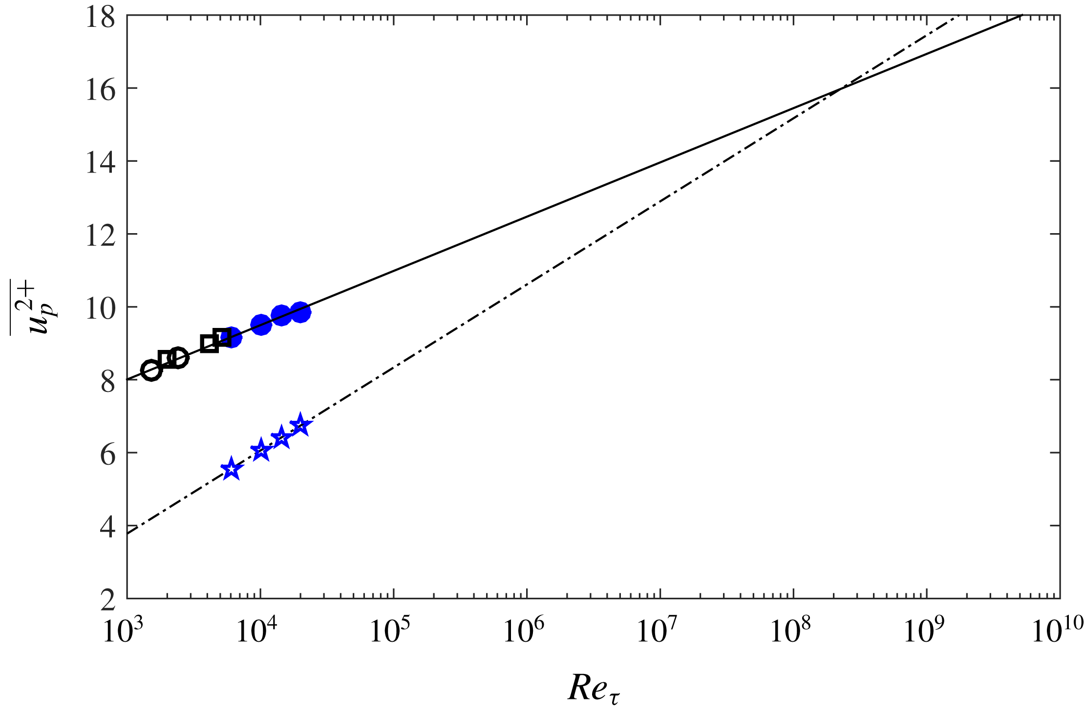
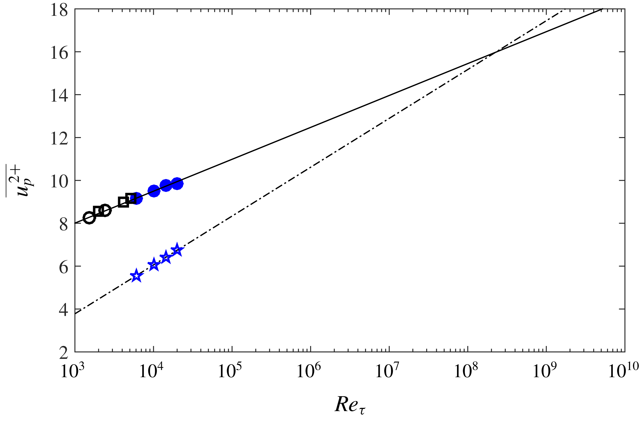
Equations (3.2) and (3.3a ) can be used to predict whether, at sufficiently high $Re_{\unicode[STIX]{x1D70F}}$ , the outer peak overcomes the inner peak. The extrapolated results in figure 8 show that such a phenomenon happens around $Re_{\unicode[STIX]{x1D70F}}=10^{8}$ . Note that since we are using an upper bound for the outer peak, i.e. (3.3a ), this is a lower bound for the predicted $Re_{\unicode[STIX]{x1D70F}}$ . In fact, as recently discussed by Marusic, Baars & Hutchins (Reference Marusic, Baars and Hutchins2017), if we adopt the near-wall peak slope in (3.2) following a gradient of $A_{1}/2$ ( $A_{1}$ is the slope in the logarithmic relation in (3.1)), then the outer peak will never reach the inner peak. Furthermore, one should acknowledge that these predictions are valid if the inner and the outer peak trends remain unchanged up to these extreme values for $Re_{\unicode[STIX]{x1D70F}}$ . Such questions remain controversial since accurate near-wall measurements up to high $Re_{\unicode[STIX]{x1D70F}}$ face significant challenges (Morrison et al. Reference Morrison, McKeon, Jiang and Smits2004; Metzger et al. Reference Metzger, McKeon and Holmes2007; Marusic, Mathis & Hutchins Reference Marusic, Mathis and Hutchins2010a ; Hultmark et al. Reference Hultmark, Vallikivi, Bailey and Smits2012). This makes any prospect of this phenomenon tentative. Nonetheless, according to the NSTAP data and the atmospheric surface layer data of Metzger & Klewicki (Reference Metzger and Klewicki2001), it is unlikely that this phenomenon happens at laboratory scale or any terrestrial $Re_{\unicode[STIX]{x1D70F}}$ .

3.2 Spatial resolution filtering of turbulence intensity in near-wall region

Several correction schemes for spatial filtering of single component hot-wire measurements have been proposed recently (Monkewitz, Duncan & Nagib Reference Monkewitz, Duncan and Nagib2010; Chin et al. Reference Chin, Hutchins, Ooi and Marusic2011; Segalini et al. Reference Segalini, Örlü, Schlatter, Alfredsson, Rüedi and Talamelli2011; Smits et al. Reference Smits, Monty, Hultmark, Bailey, Hutchins and Marusic2011; Philip et al. Reference Philip, Hutchins, Monty and Marusic2013). Comparisons of these corrections are given by Miller, Estejab & Bailey (Reference Miller, Estejab and Bailey2014). Here we restrict our assessment to the correction scheme of Smits et al. (Reference Smits, Monty, Hultmark, Bailey, Hutchins and Marusic2011).

Figure 9.

Streamwise turbulence intensity measured with the hot-wires and the NSTAP probes at various $Re_{\unicode[STIX]{x1D70F}}$ . ——, uncorrected hot-wire data; $\cdots \cdots$ , corrected hot-wire data for spatial resolution using the scheme proposed by Smits et al. (Reference Smits, Monty, Hultmark, Bailey, Hutchins and Marusic2011);

, NSTAP, $Re_{\unicode[STIX]{x1D70F}}=6000$ ; 

, NSTAP, $Re_{\unicode[STIX]{x1D70F}}=10\,000$ ; 

, NSTAP, $Re_{\unicode[STIX]{x1D70F}}=14\,500$ ; 

, NSTAP, $Re_{\unicode[STIX]{x1D70F}}=20\,000$ . (a) $Re_{\unicode[STIX]{x1D70F}}=6000$ , (b) $Re_{\unicode[STIX]{x1D70F}}=10\,000$ , (c) $Re_{\unicode[STIX]{x1D70F}}=14\,500$ , (d) $Re_{\unicode[STIX]{x1D70F}}=20\,000$ .

Figure 9 shows $\overline{{u^{2}}^{+}}$ as measured with the NSTAP and the $2.5~\unicode[STIX]{x03BC}\text{m}$ diameter hot-wire together with the Smits et al. (Reference Smits, Monty, Hultmark, Bailey, Hutchins and Marusic2011) corrected hot-wire profiles for various $Re_{\unicode[STIX]{x1D70F}}$ . It is noted that the NSTAP results are not corrected for spatial resolution since their associated $l^{+}$ is small enough to ensure that all the small-scale energy content is resolved. It can be seen that the correction works reasonably well for measurements at $Re_{\unicode[STIX]{x1D70F}}=6000$ , 10 000 and 14 500 where the inner normalised hot-wire length $l_{HW}^{+}\approx 20$ . However, for $Re_{\unicode[STIX]{x1D70F}}=20\,000$ with $l_{HW}^{+}=29$ , its performance degrades, resulting in an underestimation of the turbulence intensity around the inner peak ( $z^{+}=15$ ). Our results indicate that this correction scheme (validated for up to $Re_{\unicode[STIX]{x1D70F}}=10\,000$ in the original paper) works well for $Re_{\unicode[STIX]{x1D70F}}$ up to at least 14 500 but may not be as accurate for higher Reynolds numbers.

3.3 Skewness and kurtosis

For completeness we also show skewness ( $S_{u}$ ) and kurtosis ( $K_{u}$ ) profiles of the streamwise velocity signals against inner-scaled wall distance $z^{+}$ in figures 10(a) and 10(b). In these figures, skewness and kurtosis as measured by the NSTAP and the $2.5~\unicode[STIX]{x03BC}\text{m}$ diameter conventional hot-wire are compared at various Reynolds numbers. It appears that spatial resolution affects both $S_{u}$ and $K_{u}$ in the near-wall region up to $z^{+}\approx 200$ , but beyond this ( $z^{+}>200$ ) good agreement is observed between the NSTAP and the conventional hot-wire. These results are consistent with the observations of Talamelli et al. (Reference Talamelli, Segalini, Örlü, Schlatter and Alfredsson2013) about the effect of spatial filtering on the skewness and kurtosis in turbulent wall-bounded flows. It should also be noted that in the skewness profiles, a near-wall negative region (which diminishes with $Re_{\unicode[STIX]{x1D70F}}$ ) is seen in the NSTAP results for all the Reynolds numbers, while the conventional hot-wire cannot resolve this due to spatial filtering.

Figure 10.

Comparison of (a) skewness, $S_{u}$ , and (b) kurtosis, $K_{u}$ , as measured by $2.5~\unicode[STIX]{x03BC}\text{m}$ diameter hot-wires (——) and the NSTAP at various $Re_{\unicode[STIX]{x1D70F}}$ . Reynolds numbers are $Re_{\unicode[STIX]{x1D70F}}=6000$ (

), 10 000 (

), 14 500 (

) and 20 000 (

) and the arrow direction indicates the increase in $Re_{\unicode[STIX]{x1D70F}}$ . Skewness and kurtosis curves have been shifted in the ordinate axis for clarity.

3.4 Energy spectra

3.4.1 Near-wall region

We start this section with a dimensional analysis for the streamwise energy spectrum $\unicode[STIX]{x1D719}_{uu}$ in the near-wall region. This analysis is similar to that presented by Perry, Henbest & Chong (Reference Perry, Henbest and Chong1986) for the logarithmic wall region; however, we apply it to the near-wall region. The spectrum can be separated into three wavenumber domains.

1. (i) Small wavenumber (large wavelength) motions. In this domain, although near the wall, the boundary layer thickness is important since the contributing large-scale motions are of the order of the boundary layer thickness, $\unicode[STIX]{x1D6FF}$ . Hence, the relevant variables are energy spectrum $\unicode[STIX]{x1D719}_{uu}$ , streamwise wavenumber $k_{x}$ , friction velocity $u_{\unicode[STIX]{x1D70F}}$ , kinematic viscosity $\unicode[STIX]{x1D708}$ , wall distance $z$ and boundary layer thickness $\unicode[STIX]{x1D6FF}$ . A dimensional analysis leads to

   (3.5) $$\begin{eqnarray}{\displaystyle \frac{k_{x}\unicode[STIX]{x1D719}_{uu}}{u_{\unicode[STIX]{x1D70F}}^{2}}}=\,f_{1}(k_{x}z,z^{+},z/\unicode[STIX]{x1D6FF})=\,f_{1}(k_{x}^{+}z^{+},z^{+},z^{+}/\unicode[STIX]{x1D6FF}^{+}).\end{eqnarray}$$
   Equation (3.5) implies that in the near-wall region over the small wavenumber domain, $k_{x}\unicode[STIX]{x1D719}_{uu}/u_{\unicode[STIX]{x1D70F}}^{2}$ is dependent on $Re_{\unicode[STIX]{x1D70F}}$ as well as $k_{x}^{+}$ and $z^{+}$ .

2. (ii) Moderate to high wavenumber (moderate to small wavelength) motions. In this wavenumber domain in the near-wall region, the relevant variables are $\unicode[STIX]{x1D719}_{uu}$ , $k_{x}$ , $u_{\unicode[STIX]{x1D70F}}$ , $z$ and $\unicode[STIX]{x1D708}$ . Here, since $z/\unicode[STIX]{x1D6FF}\ll 1$ for sufficiently high $Re_{\unicode[STIX]{x1D70F}}$ , $\unicode[STIX]{x1D6FF}$ is not important. Therefore, a dimensional analysis yields

   (3.6) $$\begin{eqnarray}{\displaystyle \frac{k_{x}\unicode[STIX]{x1D719}_{uu}}{u_{\unicode[STIX]{x1D70F}}^{2}}}=\,f_{2}(k_{x}z,z^{+})=\,f_{2}(k_{x}^{+}z^{+},z^{+}).\end{eqnarray}$$
   Therefore, in this domain $k_{x}\unicode[STIX]{x1D719}_{uu}/u_{\unicode[STIX]{x1D70F}}^{2}$ can be expressed in terms of $k^{+}$ and $z^{+}$ only.

3. (iii) Very high wavenumber (very small wavelength) motions. In this range of motions, $\unicode[STIX]{x1D719}_{uu}$ is dependent on wavenumber $k_{x}$ , Kolmogorov’s length scale $\unicode[STIX]{x1D702}$ and Kolmogorov’s velocity scale $v_{\unicode[STIX]{x1D702}}$ . Here, $v_{\unicode[STIX]{x1D702}}=(\unicode[STIX]{x1D708}\unicode[STIX]{x1D716})^{1/4}$ and $\unicode[STIX]{x1D702}=(\unicode[STIX]{x1D708}^{3}/\unicode[STIX]{x1D716})^{1/4}$ , where $\unicode[STIX]{x1D708}$ is kinematic viscosity and $\unicode[STIX]{x1D716}$ is the dissipation rate. With these variables two non-dimensional parameters can be considered such that

   (3.7) $$\begin{eqnarray}{\displaystyle \frac{k_{x}\unicode[STIX]{x1D719}_{uu}}{v_{\unicode[STIX]{x1D702}}^{2}}}=\,f_{3}(k_{x}\unicode[STIX]{x1D702})=\,f_{3}(k_{x}^{+}\unicode[STIX]{x1D702}^{+}).\end{eqnarray}$$
   It is shown in appendix B that in the near-wall region and the inertial sublayer, $\unicode[STIX]{x1D702}^{+}$ and $v_{\unicode[STIX]{x1D702}}^{+}$ can be expressed as functions of inner normalised wall distance $z^{+}$ , independent of $Re_{\unicode[STIX]{x1D70F}}$ , i.e. $\unicode[STIX]{x1D702}^{+}=h_{\unicode[STIX]{x1D702}}(z^{+})$ and $v_{\unicode[STIX]{x1D702}}^{+}=h_{v}(z^{+})$ . Therefore, equation (3.7) can be rewritten as
   (3.8) $$\begin{eqnarray}{\displaystyle \frac{k_{x}\unicode[STIX]{x1D719}_{uu}}{u_{\unicode[STIX]{x1D70F}}^{2}}}=[h_{v}(z^{+})]^{2}f_{3}(k_{x}^{+}h_{\unicode[STIX]{x1D702}}(z^{+})),\end{eqnarray}$$
   which shows that in this wavenumber domain, similar to moderate to high wavenumber motions, $k_{x}\unicode[STIX]{x1D719}_{uu}/u_{\unicode[STIX]{x1D70F}}^{2}$ is a function of $k^{+}$ and $z^{+}$ and independent of $Re_{\unicode[STIX]{x1D70F}}$ .

Figure 11.

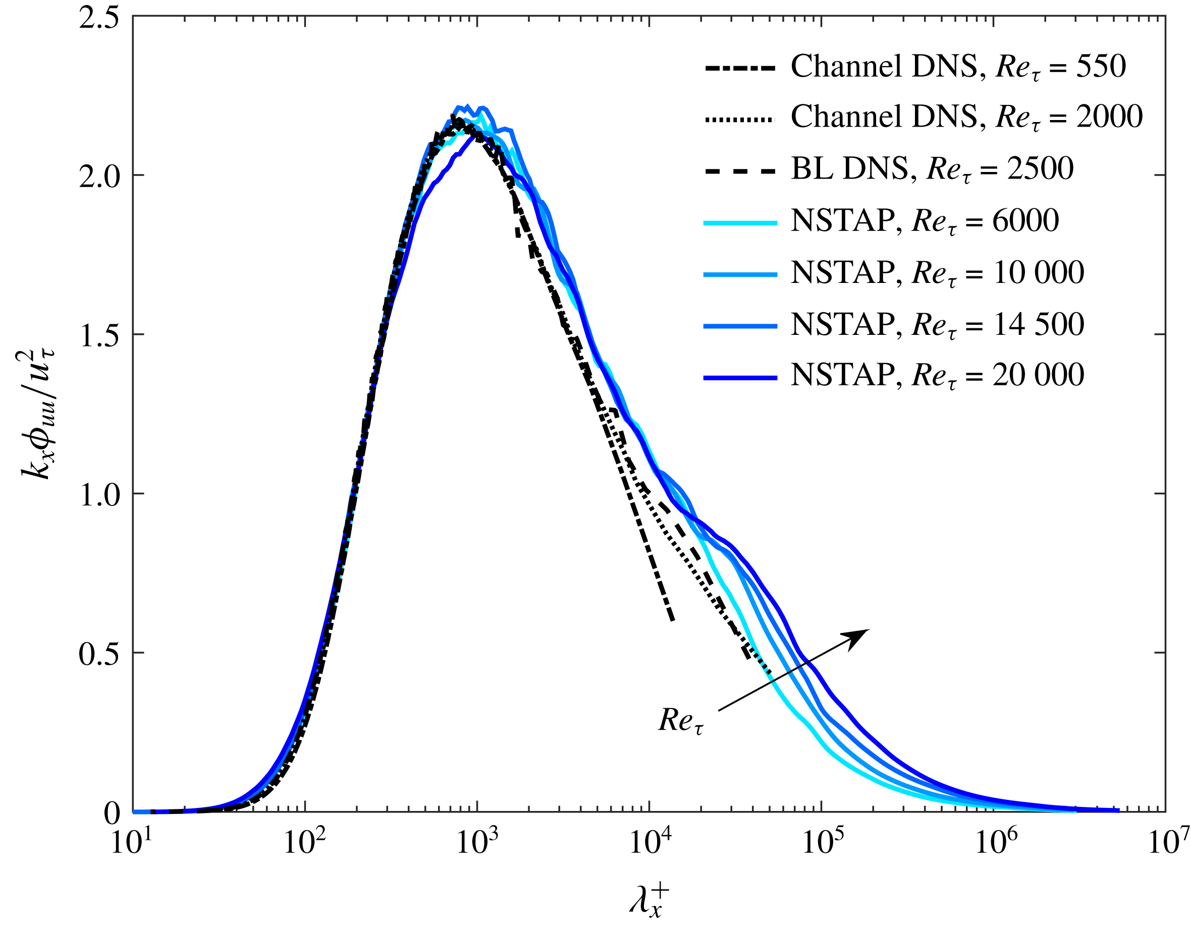
Comparison of pre-multiplied energy spectra at $z^{+}\approx 15$ from various Reynolds numbers and flow geometries. The arrow indicates increase in $Re_{\unicode[STIX]{x1D70F}}$ for the NSTAP spectra.

The above arguments indicate that at a fixed $z^{+}$ in the near wall, $k_{x}\unicode[STIX]{x1D719}_{uu}(k^{+})/u_{\unicode[STIX]{x1D70F}}^{2}$ (or equivalently $k_{x}\unicode[STIX]{x1D719}_{uu}(\unicode[STIX]{x1D706}_{x}^{+})/u_{\unicode[STIX]{x1D70F}}^{2}$ where $\unicode[STIX]{x1D706}_{x}=2\unicode[STIX]{x03C0}/k_{x}$ is the wavelength) curves should collapse over medium to very high wavenumbers (medium to very low wavelengths) when various $Re_{\unicode[STIX]{x1D70F}}$ are compared, and $Re_{\unicode[STIX]{x1D70F}}$ dependence is expected in the low wavenumber (high wavelength) end of the spectra only. Since small-scale energy can be significantly affected by spatial resolution (as documented by Chin et al. (Reference Chin, Hutchins, Ooi and Marusic2009) and Hutchins et al. (Reference Hutchins, Nickels, Marusic and Chong2009)), the data here may be helpful to clarify the small-scale behaviour in the near wall. The inner-scaled, pre-multiplied energy spectra $k_{x}\unicode[STIX]{x1D719}_{uu}/u_{\unicode[STIX]{x1D70F}}^{2}$ are plotted against streamwise wavelength, $\unicode[STIX]{x1D706}_{x}^{+}$ , in figure 11 at the peak turbulence intensity location, $z^{+}\approx 15$ for the experimental data ( $Re_{\unicode[STIX]{x1D70F}}=6000$ , 10 000, 14 500 and 20 000) as well as channel DNS data of Hoyas & Jiménez (Reference Hoyas and Jiménez2006) at $Re_{\unicode[STIX]{x1D70F}}=550$ , 2000 and boundary layer DNS data of Sillero et al. (Reference Sillero, Jiménez and Moser2013) at $Re_{\unicode[STIX]{x1D70F}}=2500$ . Taylor’s frozen turbulence hypothesis (Taylor Reference Taylor1938) is employed to deduce spatial spectra from the time series data obtained from the stationary hot-wire for the experimental spectra, while spatial information is used to construct spectra from DNS. Here, spectra are plotted in pre-multiplied form so that equal areas equate to equal contributions to the turbulence intensities on the semilogorithmic plot: $\int _{0}^{\infty }\unicode[STIX]{x1D719}_{uu}\,\text{d}k_{x}=\int _{0}^{\infty }k_{x}\unicode[STIX]{x1D719}_{uu}\,\text{d}(\log k_{x})=\int _{0}^{\infty }k_{x}\unicode[STIX]{x1D719}_{uu}\,\text{d}(\log \unicode[STIX]{x1D706}_{x})=\overline{u^{2}}$ .

All the spectra appear to collapse well for the wavelengths below $\unicode[STIX]{x1D706}_{x}^{+}\approx 700$ and the experimental spectra ( $Re_{\unicode[STIX]{x1D70F}}\geqslant 6000$ ) collapse well for the wavelengths below $\unicode[STIX]{x1D706}_{x}^{+}\approx 15\,000$ . This is consistent with the dimensional analysis. Moreover, in the high wavelength end of the spectra an increasing trend with $Re_{\unicode[STIX]{x1D70F}}$ is evident. These observations are consistent with the experimental study of Hutchins et al. (Reference Hutchins, Nickels, Marusic and Chong2009) in the boundary layer flow (up to $Re_{\unicode[STIX]{x1D70F}}\approx 19\,000$ ) where hot-wire sensors with lengths of 22 wall units were used, and for the lower Reynolds number DNS studies of Hoyas & Jiménez (Reference Hoyas and Jiménez2006) (up to $Re_{\unicode[STIX]{x1D70F}}\approx 2000$ ) in the channel flow, and Chin, Monty & Ooi (Reference Chin, Monty and Ooi2014) (up to $Re_{\unicode[STIX]{x1D70F}}\approx 2000$ ) in the pipe flow. It is not clear why the DNS and the experimental spectra diverge for $10^{3}<\unicode[STIX]{x1D706}_{x}^{+}<10^{4}$ . This may be due to use of Taylor’s frozen turbulence hypothesis in experimental spectra. The peak of the inner normalised pre-multiplied energy spectra is seen to remain constant at $k_{x}\unicode[STIX]{x1D719}_{uu}/u_{\unicode[STIX]{x1D70F}}^{2}\approx 2.2$ at the inner normalised wavelength $\unicode[STIX]{x1D706}_{x}^{+}\approx 850$ within measurement uncertainty. It should also be noted that the small-scale energy is not only invariant with $Re_{\unicode[STIX]{x1D70F}}$ but independent of the flow geometry, since channel and boundary layer flow spectra in the small-scale region appear to collapse well. This behaviour in the $u$ -spectra at $z^{+}\approx 15$ explains the increasing trend with $Re_{\unicode[STIX]{x1D70F}}$ for the peak $\overline{{u^{2}}^{+}}$ in the near-wall region; there is an increasing amount of large-scale superimposed energy as $Re_{\unicode[STIX]{x1D70F}}$ increases while the small-scale energy content appears to be universal. Figure 12 shows the same plots for the experimental data at other inner normalised wall distance locations. It can be seen that the $k_{x}\unicode[STIX]{x1D719}_{uu}/u_{\unicode[STIX]{x1D70F}}^{2}$ curves collapse for wavelengths below $\unicode[STIX]{x1D706}_{x}^{+}\approx 15\,000$ up to $z^{+}=280$ for the Reynolds number range $6000\leqslant Re_{\unicode[STIX]{x1D70F}}\leqslant 20\,000$ .

Figure 12.

Reynolds number dependence of pre-multiplied energy spectra as measured with the NSTAP at (a) $z^{+}\approx 24$ , (b) $z^{+}\approx 92$ , (c) $z^{+}\approx 180$ , (d) $z^{+}\approx 280$ . Lines are as in figure 11. The arrow indicates increase in $Re_{\unicode[STIX]{x1D70F}}$ .

3.4.2 The $k_{x}^{-5/3}$ power scaling law

Figure 13.

Compensated Kolmogorov’s universal scaling for the streamwise energy spectra at $Re_{\unicode[STIX]{x1D70F}}=6000$ , 10 000, 14 500, 20 000 at (a) $z/\unicode[STIX]{x1D6FF}\approx 0.05$ , (b) $z/\unicode[STIX]{x1D6FF}\approx 0.1$ , (c) $z/\unicode[STIX]{x1D6FF}\approx 0.15$ , (d) $z/\unicode[STIX]{x1D6FF}\approx 0.4$ . Saddoughi & Veeravalli (Reference Saddoughi and Veeravalli1994) found the Kolmogorov constant to be $K_{0}=0.49$ , which is slightly higher than our result which is $K_{0}=0.48$ . The arrow indicates increase in $Re_{\unicode[STIX]{x1D70F}}$ .

Hutchins et al. (Reference Hutchins, Nickels, Marusic and Chong2009) have shown that limited spatial resolution of hot-wires can affect the $k_{x}^{-5/3}$ power scaling region by attenuating the so-called ‘spectral bump’ in the Kolmogorov-scaled energy spectra (Saddoughi & Veeravalli Reference Saddoughi and Veeravalli1994), resulting in misleading estimates of $-5/3$ regions. Here, the NSTAP length is shorter than the Kolmogorov length scale in the logarithmic and outer regions where $k_{x}^{-5/3}$ power scaling is expected to hold (see figure 17(a) for inner normalised Kolmogorov length scale values across the boundary layer thickness at varying $Re_{\unicode[STIX]{x1D70F}}$ ); hence, we inspect this scaling across a range of Reynolds numbers in turbulent boundary layers. The mean rate of turbulent kinetic energy dissipation ( $\unicode[STIX]{x1D716}$ ) is estimated using local isotropy, which allows $\unicode[STIX]{x1D716}$ to be determined from integration of the one-dimensional dissipation spectrum $D(k_{x})$ (Townsend Reference Townsend1976), i.e.

(3.9) $$\begin{eqnarray}\unicode[STIX]{x1D716}=15\unicode[STIX]{x1D708}\int _{0}^{\infty }D(k_{x})\,\text{d}k_{x}=15\unicode[STIX]{x1D708}\int _{0}^{\infty }k_{x}^{2}\unicode[STIX]{x1D719}_{uu}\,\text{d}k_{x}.\end{eqnarray}$$

Figure 13 shows the compensated Kolmogorov-scaled streamwise energy spectra at four outer-scaled wall-normal locations for various Reynolds numbers. The $-5/3$ scaling law appears as a horizontal line in this form of compensated spectra. One can see that a clear $-5/3$ scaling is elusive for $z/\unicode[STIX]{x1D6FF}\leqslant 0.15$ , i.e. the logarithmic region, in the $Re_{\unicode[STIX]{x1D70F}}$ range of this study. Only at $z/\unicode[STIX]{x1D6FF}=0.4$ , which is located in the wake region, are apparent regions of plateau observed. Vallikivi et al. (Reference Vallikivi, Ganapathisubramani and Smits2015a ), however, found that for high Reynolds number turbulent boundary layer and pipe flows at $z/\unicode[STIX]{x1D6FF}=0.5$ , energy spectra have an exponent that is closer to $-1.5$ than to $-5/3$ . The plateau level in our results, which equates to Kolmogorov’s constant $K_{0}$ , changes with $Re_{\unicode[STIX]{x1D70F}}$ from 0.52 for $Re_{\unicode[STIX]{x1D70F}}=6000$ to 0.48 for $Re_{\unicode[STIX]{x1D70F}}=14\,500$ and 20 000 (the plateau values are determined by fitting a horizontal line to the flat portions of the compensated spectra at $z/\unicode[STIX]{x1D6FF}=0.4$ ). This is probably because in the lower $Re_{\unicode[STIX]{x1D70F}}$ cases, the separation between large energetic scales and small dissipative scales is insufficient. The Kolmogorov constant for the highest $Re_{\unicode[STIX]{x1D70F}}$ ( $K_{0}=0.48$ ) is slightly lower than that reported by Saddoughi & Veeravalli (Reference Saddoughi and Veeravalli1994) ( $K_{0}=0.49$ ) in their extremely high- $Re_{\unicode[STIX]{x1D70F}}$ boundary layer experiment. This insufficient scale separation might be part of the reason for the weak Reynolds number dependence of the Kolmogorov constant reported in the literature (Sreenivasan Reference Sreenivasan1995).

3.4.3 Spectrograms

Figure 14.

Pre-multiplied spectra for the streamwise velocity $k_{x}\unicode[STIX]{x1D719}_{uu}/u_{\unicode[STIX]{x1D70F}}$ against inner-scaled wavelength $\unicode[STIX]{x1D706}_{x}^{+}$ and wall distance $z^{+}$ at (a) $Re_{\unicode[STIX]{x1D70F}}=6000$ , (b) $Re_{\unicode[STIX]{x1D70F}}=10\,000$ , (c) $Re_{\unicode[STIX]{x1D70F}}=14\,500$ and (d) $Re_{\unicode[STIX]{x1D70F}}=20\,000$ . ‘+’ indicates the inner energy site.

Figure 15.

Iso-contours of $k_{x}\unicode[STIX]{x1D719}_{uu}/u_{\unicode[STIX]{x1D70F}}^{2}$ against (a) inner-scaled wavelength $\unicode[STIX]{x1D706}_{x}^{+}$ and wall distance $z^{+}$ at the contour levels of 2, 1.4, 0.9, 0.68 and 0.45, (b) $\unicode[STIX]{x1D6FF}$ -scaled wave length $\unicode[STIX]{x1D706}_{x}/\unicode[STIX]{x1D6FF}$ and wall distance $z/\unicode[STIX]{x1D6FF}$ at the contour levels of 0.9, 0.68 and 0.45 for various $Re_{\unicode[STIX]{x1D70F}}$ . Reynolds numbers are 6000 (

), 10 000 (

), 14 500 (

) and 20 000 (

).

In an attempt to provide an overview of the energy distribution across various wavelengths and wall distances, and also the effect of $Re_{\unicode[STIX]{x1D70F}}$ on the energy distribution, contour maps of the pre-multiplied energy spectra $k_{x}\unicode[STIX]{x1D719}_{uu}/u_{\unicode[STIX]{x1D70F}}^{2}$ are plotted against inner-scaled wall distance ( $z^{+}$ ) and inner-scaled streamwise wavelength in figure 14 for $Re_{\unicode[STIX]{x1D70F}}=6000{-}20\,000$ . Here the magnitude of $k_{x}\unicode[STIX]{x1D719}_{uu}/u_{\unicode[STIX]{x1D70F}}^{2}$ is indicated using colour variations. These contour maps show a distinct near-wall peak in the spectrogram for all Reynolds numbers (indicated with white ‘+’ symbols) known as the ‘inner energy site’, which occur at a nominally fixed inner-scaled wall distance $z^{+}\approx 13$ and inner-scaled wavelength $\unicode[STIX]{x1D706}_{x}^{+}\approx 1000$ at a fixed energy level $k_{x}\unicode[STIX]{x1D719}_{uu}/u_{\unicode[STIX]{x1D70F}}^{2}\approx 2.2$ . This wall distance corresponds to approximately the peak in the broadband turbulence intensity, and is related to the near-wall energetic cycle of streaks and quasi-streamwise vortices (Kline et al. Reference Kline, Reynolds, Schraub and Runstadler1967; Jiménez & Pinelli Reference Jiménez and Pinelli1999). In order to acquire better comprehension of the $Re_{\unicode[STIX]{x1D70F}}$ effect on the near-wall energy spectral density, iso-contours of pre-multiplied energy for the spectral surfaces shown previously are now shown in figure 15(a) for various $Re_{\unicode[STIX]{x1D70F}}$ . Five contour levels corresponding to $k_{x}\unicode[STIX]{x1D719}_{uu}/u_{\unicode[STIX]{x1D70F}}^{2}=0.45,0.68,0.9,1.4$ and 2 are shown, and colour gradients are used to indicate $Re_{\unicode[STIX]{x1D70F}}$ variations. The four sets of contours (four Reynolds numbers) show very good collapse on the left-hand side of the inclined dashed line. However, if we look to the right of the dashed line, it is evident that there is an increasing amount of high wavelength energy with $Re_{\unicode[STIX]{x1D70F}}$ extending across all wall heights. This high wavelength energy in the near-wall region is the footprint of an emergent ‘outer energy site’, growth of which with $Re_{\unicode[STIX]{x1D70F}}$ is evident in figure 14. Hutchins & Marusic (Reference Hutchins and Marusic2007) reported emergence of an outer peak associated with this outer energy site at higher Reynolds numbers, and Mathis, Hutchins & Marusic (Reference Mathis, Hutchins and Marusic2009) later proposed the location of the peak to be $Re_{\unicode[STIX]{x1D70F}}$ dependent as $z^{+}\approx \sqrt{15Re_{\unicode[STIX]{x1D70F}}}$ , which coincides with the geometric centre of the logarithmic region. More recently, Vallikivi et al. (Reference Vallikivi, Ganapathisubramani and Smits2015a ) reported that the location of the outer spectral peak at high Reynolds numbers marks the start of a broad plateau. This latter observation is consistent with the outer spectral region at $Re_{\unicode[STIX]{x1D70F}}=20\,000$ in our results. However, $Re_{\unicode[STIX]{x1D70F}}=20\,000$ is only sufficient to see the emergence of this broad plateau which would be expected from the results of Vallikivi et al. (Reference Vallikivi, Ganapathisubramani and Smits2015a ) to become more prominent at higher Reynolds numbers. Figure 15(b) shows a Reynolds number comparison of three contour levels corresponding to $k_{x}\unicode[STIX]{x1D719}_{uu}/u_{\unicode[STIX]{x1D70F}}^{2}=0.45,0.68,0.9$ against outer-scaled wavelength and wall distance. It is evident that the outer-scaled spectra collapse well in the outer region (showing existence of an outer-scaling similarity) and gradually separate at lower $z/\unicode[STIX]{x1D6FF}$ and $\unicode[STIX]{x1D706}_{x}/\unicode[STIX]{x1D6FF}$ . This is consistent with the attached eddy hypothesis model of Perry et al. (Reference Perry, Henbest and Chong1986).