1. Introduction
The filling and simultaneous natural emptying of a box (subject to a continuous supply of buoyancy) is a problem of interest in building engineering. Typical applications include thermal comfort, indoor air quality, accidental gas release and fire smoke management, to name but a few. This buoyancy-driven flow is of practical importance in estimating the temperature (or concentration) distribution in a box during the transients and at steady state, the flow rates through the box openings, the time required to reach steady state, and so on. Another important consideration is whether the flow pattern exhibits stratification or not, which depends on the geometrical configuration and the source buoyancy flux. Beyond building applications, a recent article by Roes, Bolster & Flynn (Reference Roes, Bolster and Flynn2014) addresses, with a similar mathematical formalism, the problem of contamination (or filtration) through a porous medium. More anecdotally, filling–emptying problems also occur in physiology (e.g. in the lung or bladder) even if processes here are rarely both continuous and simultaneous.
Independently of the emptying process, the filling of a box by a buoyant source located on the floor was first examined theoretically by Baines & Turner (Reference Baines and Turner1969) on the basis of Morton’s plume theory (Morton, Taylor & Turner Reference Morton, Taylor and Turner1956). In their model (known as the ‘filling box’ model), these authors considered that the buoyant plume rises, impinges on the top of the box and flows along it to form a thin layer at the beginning of the filling process. This layer is then continuously fed (at the density interface formed between the layer and the ambient fluid) by the plume and grows monotonically but increasingly slowly over time. This ‘filling box’ model assumes the existence of a stratification that is sharp (a homogeneous light fluid layer over homogeneous ambient fluid) or stable with a density profile in the buoyant upper layer fixed in shape and changing at a uniform rate in time at all levels. Significant evolutions to represent the actual density profile in the upper layer were proposed by several authors, particularly Worster & Huppert (Reference Worster and Huppert1983).
The draining of a light fluid layer through an opening located at the top of a box is a straightforward problem to solve as long as Bernoulli’s theorem applies. In particular, a horizontally uniform density in the drained fluid layer is required over a succession of quasi-steady states. This assumption, which corresponds to a situation of ideal displacement flow, is questionable when the replacement fluid (at ambient density) entering at the base opening of the box creates a jet that disrupts the interface or when the base opening is so small that bidirectional flow occurs at the top (draining) opening. The dynamics of such ‘emptying boxes’ were analysed in detail by Coffey & Hunt (Reference Coffey and Hunt2010) and Hunt & Coffey (Reference Hunt and Coffey2010). Following the scalings derived by these authors from their experiments, it can be considered that true classical displacement flows (unidirectional without interface mixing) exist if the inlet area (for incoming ambient air) is about three to four times larger than the outlet area.
The simultaneous emptying and filling (by a source of buoyancy) of a box was first studied both theoretically and experimentally by Linden, Lane-Serff & Smeed (Reference Linden, Lane-Serff and Smeed1990). In the case of a strong stable stratification (displacement ventilation), these authors formally determined the upper layer thickness
 $h_{ss}$
at steady state. As their approach was restricted to Boussinesq plumes, they demonstrated that
 $h_{ss}$
could be considered as independent of the strength of the buoyant source, being a function of only a single geometrical parameter. This ‘emptying–filling box’ theory was later extended to take into account effects of the marked density contrasts characteristic in fires (Rooney & Linden Reference Rooney and Linden1997), external wind (Hunt & Linden Reference Hunt and Linden2001; Mott & Woods Reference Mott and Woods2012), heat transfers (Lane-Serff & Sandbach Reference Lane-Serff and Sandbach2012) and multiple sources of differing strength (Shrinivas & Hunt Reference Shrinivas and Hunt2014).
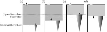
As in the filling box problem, in a box that is simultaneously filling and emptying, a light (or hot) fluid layer forms whose interface descends towards the plume over time. The main difference is that a first equilibrium state can be obtained as soon as the volume flow rate of the plume through the interface (filling flow) balances the volume flow rate of the fluid naturally draining at the top opening (draining flow). Nevertheless, when the interface has reached this position (see figure 1 a), the upper layer is supplied with a reduced volume flux and excessively buoyant fluid, so the hydrostatic pressure difference increases. As a result, the volume flux out of the upper opening exceeds that supplied by the plume and the interface may then move upwards (see figure 1 b). This is why the height of the interface at the first equilibrium state may be regarded as an ‘overshoot’ when it is compared with the height of the interface at its (final) steady state. The ‘overshoot’ phenomenon was first identified by Hunt & Linden (Reference Hunt, Linden, Mundt and Malmstrom1998) and later examined both theoretically and experimentally (salt-water experiments) in Kaye & Hunt (Reference Kaye and Hunt2004). These authors explained the phenomenon by considering (under the right conditions) a fast thickening of the upper layer so that the interface reaches the steady state height before the draining flow can balance the filling flow. In the same way, an upward ‘overshoot’ (see figure 1 c) can be explained, under the right conditions, by a fast thinning of the upper layer so that the interface reaches the steady state height before the filling flow can balance the draining flow. The upper layer is then supplied with an excessive volume flux and fluid of reduced buoyancy so the interface may move downwards (see figure 1 d). The process may then continue, leading the interface to oscillate around its final height before reaching it.
Sketch of a possible oscillation of the upper layer interface: (a) at the downward ‘overshoot’ the filling flow from the plume balances the upper opening flow, (b) the difference in draining hydrostatic pressure has increased and the interface moves up, (c) at the possible upward ‘overshoot’ the filling flow from the plume again balances the upper opening flow, (d) the draining hydrostatic pressure has decreased and the interface moves down.

Multiple overshoots leading to oscillations have not previously been reported. The objective of this study is to demonstrate that such oscillations are theoretically possible, and then determine their period and damping. For mathematical simplicity, the case of a line plume is considered. In § 2, the configuration studied, the hypothesis, the governing equations and steady-state solutions of the problem are presented. In § 3, the governing equations are linearized around the steady state in order to get a second-order differential equation from which the existence of damped oscillations is deduced, quantified and discussed. An extension for (point source) round plumes is presented in the appendix A.
2. Configuration and governing equations
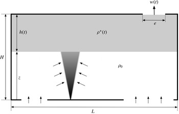
As shown in figure 2, we consider the simultaneous filling and emptying of a cuboid box. The box height is
 $H$
and its constant horizontal surface is
 $L\times l$
(width
 $\times$
depth). The box is continuously supplied with buoyant fluid from a plane plume (extending throughout the box depth) of given buoyancy flux
 $B$
(defined per unit of depth) and naturally emptied through a 2D horizontal opening in its top of width
 $e$
(and depth
 $l$
). At a given time, the outflow mean velocity at the top opening is denoted
 $w$
,
 $h$
represents the thickness of the buoyant upper layer that develops in the box and
 ${\it\rho}^{\ast }$
its density. This density is considered as constant since the buoyant upper layer is assumed to be ‘well mixed’ in the steady state as well as during the transient. It is also assumed that the base openings (for the incoming ambient air at density
 ${\it\rho}_{0}$
) are large enough to overcome the specific behaviours mentioned in § 1 (inlet jet strongly mixing the interface and bidirectional flows at the openings). Finally, to ensure an ideal filling box flow, the box aspect ratio
 $H/L$
is considered sufficiently small that the effect of the plume ‘overturning’, caused by impingement on the sidewalls, is negligible. This condition limits our discussion to box aspect ratios less than unity (Kaye & Hunt Reference Kaye and Hunt2007).
Schematic diagram of the studied configuration.

Following the turbulent plume theory by Morton et al. (Reference Morton, Taylor and Turner1956), we model the buoyant release using the self-similar solutions of a non-Boussinesq line plume. These solutions allow the plume characteristics (mean velocity
 $u$
, thickness
 $b$
and density
 ${\it\rho}$
) to be expressed as functions of a vertical coordinate
 $z$
, thus
 $$\begin{eqnarray}u(z)=u_{i},\quad b(z)=2{\it\alpha}\frac{{\it\rho}_{0}}{{\it\rho}}z,\quad \frac{{\rm\Delta}{\it\rho}}{{\it\rho}}(z)=\frac{u_{i}^{2}}{gz},\end{eqnarray}$$
where
 $g$
is the gravitational acceleration,
 ${\it\alpha}$
is the entrainment coefficient and
 ${\rm\Delta}{\it\rho}={\it\rho}_{0}-{\it\rho}$
. Note that the (constant) vertical velocity in the plane plume
 $u_{i}$
can be calculated from the buoyancy flux
 $B$
(defined per unit of depth) as
 $u_{i}^{3}=B/2{\it\alpha}$
. It is important to underline that these solutions are obtained with an unmodified entrainment model unlike those given in the appendix A (for non-Boussinesq round plumes) in which the classical Morton’s entrainment coefficient
 ${\it\alpha}$
is multiplied by the square root of the plume local density (Rooney & Linden Reference Rooney and Linden1996). In the absence of detailed experiments for plane plumes, the non-Boussinesq effects on the entrainment velocity are usually neglected though this remains an open matter for debate (see van den Bremer & Hunt Reference van den Bremer and Hunt2014).
For area source plumes, the relations in (2.1) can be modified by introducing a virtual origin correction. From a mathematical point of view, such a modification has no direct impact on the theoretical development that follows but it will have to be considered when analysing the model results quantitatively. Therefore, a specific discussion of sources of finite area will be presented in § 3.5.
With the above assumptions, conservation equations for volume and mass flow rates in the buoyant upper layer may be expressed as
 $$\begin{eqnarray}\displaystyle & \displaystyle \frac{\text{d}(H-z)L}{\text{d}t}=bu|_{z=H-h}-we, & \displaystyle\end{eqnarray}$$
 $$\begin{eqnarray}\displaystyle & \displaystyle \frac{\text{d}{\it\rho}^{\ast }(H-z)L}{\text{d}t}=\left.{\it\rho}bu\right|_{z=H-h}-{\it\rho}^{\ast }we. & \displaystyle\end{eqnarray}$$
 ${\it\zeta}=z/H=1-h/H$
(the dimensionless height of the interface location) and
 ${\it\eta}={\rm\Delta}{\it\rho}^{\ast }/{\it\rho}^{\ast }$
(the reduced density of the upper layer). Equations (2.2) and (2.3) can be rewritten in a dimensionless form as
 $$\begin{eqnarray}\displaystyle & \displaystyle \frac{\text{d}{\it\zeta}}{\text{d}{\it\tau}}={\it\omega}{\it\varepsilon}-2{\it\alpha}{\it\lambda}({\it\zeta}+{\it\Theta}), & \displaystyle\end{eqnarray}$$
 $$\begin{eqnarray}\displaystyle & \displaystyle \frac{\text{d}{\it\eta}}{\text{d}{\it\tau}}=2{\it\alpha}{\it\lambda}\frac{1+{\it\eta}}{1-{\it\zeta}}({\it\Theta}-{\it\zeta}{\it\eta}), & \displaystyle\end{eqnarray}$$
 $$\begin{eqnarray}{\it\tau}=\frac{u_{i}}{H}t,\quad {\it\omega}=\frac{w}{u_{i}},\quad {\it\varepsilon}=\frac{e}{L},\quad {\it\lambda}=\frac{H}{L}\quad \text{and}\quad {\it\Theta}=\frac{B^{2/3}}{2{\it\alpha}^{1/3}gH}.\end{eqnarray}$$
The dimensionless parameter
 ${\it\Theta}$
corresponds in fact to the value of
 ${\it\Delta}{\it\rho}/{\it\rho}$
for
 $z=H$
(or
 ${\it\zeta}=1$
), namely the value of the reduced density
 ${\it\eta}$
in the initial layer that is formed at the ceiling at
 $t=0$
. Based on its definition above, it is worth noting that this parameter will be close to zero, especially as the buoyancy flux
 $B$
is weak and/or the box is high.
Bernoulli’s theorem applied between a point located at the interface and a point located downstream of the top opening at the vena contracta yields
 $$\begin{eqnarray}{\it\rho}^{\ast }w^{2}=2C_{d}^{2}{\rm\Delta}{\it\rho}^{\ast }gh.\end{eqnarray}$$
In this relation,
 $C_{d}$
is the discharge coefficient. For a horizontal vent, its value is generally taken to be around
 $0.7\approx 1/\sqrt{2}$
which suggests that half of the draining potential energy is dissipated by losses. This coefficient can be significantly reduced for large density contrasts as Holford & Hunt (Reference Holford, Hunt and Dally2001) have shown experimentally. For simplicity, the discharge coefficient will be assumed to be constant in the following. Note that dynamic pressure in (2.7) is expressed using the upper layer density
 ${\it\rho}^{\ast }$
and not the ambient density
 ${\it\rho}_{0}$
as in Boussinesq models. In dimensionless form, Bernoulli’s theorem becomes
 $$\begin{eqnarray}{\it\omega}^{2}=2\frac{C_{d}^{2}}{{\it\Theta}}{\it\eta}(1-{\it\zeta}).\end{eqnarray}$$
At steady state, the time-derivative terms vanish and equations (2.4), (2.5) and (2.8) can be easily combined. We then obtain the following cubic equation whose unique real root
 $\bar{{\it\zeta}}$
is the value of the variable
 ${\it\zeta}$
at steady state:
 $$\begin{eqnarray}\bar{{\it\zeta}}^{3}+2{\it\Theta}\bar{{\it\zeta}}^{2}+({\it\Theta}^{2}+{\it\Lambda})\bar{{\it\zeta}}={\it\Lambda}\quad \text{or}\quad \bar{{\it\zeta}}\,(\bar{{\it\zeta}}+{\it\Theta})^{2}={\it\Lambda}(1-\bar{{\it\zeta}}),\end{eqnarray}$$
with
 ${\it\Lambda}$
a geometrical parameter defined as
 $$\begin{eqnarray}{\it\Lambda}=\frac{C_{d}^{2}{\it\varepsilon}^{2}}{2{\it\alpha}^{2}{\it\lambda}^{2}}=\frac{C_{d}^{2}}{2{\it\alpha}^{2}}\left(\frac{e}{H}\right)^{2}.\end{eqnarray}$$
Thereafter,
 ${\it\eta}$
and
 ${\it\omega}$
at steady state are expressed as
 $$\begin{eqnarray}\bar{{\it\eta}}=\frac{{\it\Theta}}{\bar{{\it\zeta}}},\quad \bar{{\it\omega}}=\frac{C_{d}\sqrt{2}}{\sqrt{{\it\Lambda}}}(\bar{{\it\zeta}}+{\it\Theta})\quad \text{or}\quad \bar{{\it\omega}}^{2}=2C_{d}^{2}\frac{1-\bar{{\it\zeta}}}{\bar{{\it\zeta}}}.\end{eqnarray}$$
At steady state, it can be seen that
 $\bar{{\it\zeta}}$
(as well as
 $\bar{{\it\omega}}$
and
 $\bar{{\it\eta}}$
) does not depend on the box width
 $L$
, which only affects the time to reach this steady state. This is not surprising since the equilibrium imposed by the draining process depends only on layer height and density. It is then found that
 $\bar{{\it\zeta}}$
is a function of the ratio
 $e/H$
, a classical result already highlighted by Linden et al. (Reference Linden, Lane-Serff and Smeed1990) and by Kaye & Hunt (Reference Kaye and Hunt2004). Nevertheless, those authors developed their theory using the Boussinesq approximation, and concluded that layer thickness
 $h_{ss}$
does not depend on source strength. This is not true in the general non-Boussinesq case. Relation (2.9a,b
) shows that
 $\bar{{\it\zeta}}\,(=1-h_{ss}/H)$
does depend on
 $e/H$
, but also on the source buoyancy flux, via the dimensionless number
 ${\it\Theta}$
. This dependence on the source strength was already noted by Rooney & Linden (Reference Rooney and Linden1997), who addressed the emptying–filling box problem in the context of (non-Boussinesq) fire plumes.
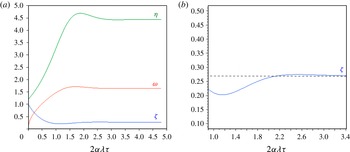
Before studying theoretically the existence of multiple overshoots and oscillations, equations (2.4), (2.5) and (2.8) were first solved numerically using the Runge–Kutta method for
 ${\it\Theta}=1.2$
and
 ${\it\Lambda}=0.8$
. Figure 3(a) shows the evolution of
 ${\it\zeta}$
,
 ${\it\eta}$
and
 ${\it\omega}$
as a function of the dimensionless time
 $2{\it\alpha}{\it\lambda}\,{\it\tau}$
. It can be seen graphically that the interface ‘overshoot’ (minimal value of
 ${\it\zeta}$
) is followed in time by a maximal value of the velocity at the top opening, and then by a maximal value of the reduced density of the upper layer (similar to the ‘thermal overshoot’ already noticed in Shrinivas & Hunt (Reference Shrinivas and Hunt2014)). Figure 3(b) is an enlargement of figure 3(a) for the variable
 ${\it\zeta}$
, which shows that, at the chosen conditions, the first (downward) ‘overshoot’ is followed by a second one (upward). The same behaviour can be also observed for the variables
 ${\it\eta}$
and
 ${\it\omega}$
.
(a) Evolution of
 ${\it\zeta}$
,
 ${\it\eta}$
and
 ${\it\omega}$
as a function of the dimensionless time
 $2{\it\alpha}{\it\lambda}\,{\it\tau}$
(for
 ${\it\Theta}=1.2$
and
 ${\it\Lambda}=0.8$
). (b) Enlargement of (a) for
 ${\it\zeta}$
just before and after the first (downward) ‘overshoot’.

3. Existence of oscillations
In this section, the governing equations are first linearized around the (final) steady state. A second-order differential equation is presented that allows us to discuss the possibility of having oscillating regimes. These oscillations are quantified, at first for the so-called ‘small plume’ and then in a general case. A short discussion on the applicability of the results for sources of finite area is also provided.
3.1. Linearization
Let us consider that instantaneous variables (
 ${\it\zeta},{\it\eta}$
and
 ${\it\omega}$
) consist of small fluctuations (denoted
 $^{\prime }$
) around a steady-state solution (denoted
 $^{-}$
):
 $$\begin{eqnarray}{\it\zeta}=\bar{{\it\zeta}}+{\it\zeta}^{\prime },\quad {\it\eta}=\bar{{\it\eta}}+{\it\eta}^{\prime },\quad {\it\omega}=\bar{{\it\omega}}+{\it\omega}^{\prime }.\end{eqnarray}$$
Equations (2.4), (2.5) and (2.8) are then linearized at the first order, leading to
 $$\begin{eqnarray}\displaystyle & \displaystyle \frac{\text{d}{\it\zeta}^{\prime }}{\text{d}{\it\tau}}=-2{\it\alpha}{\it\lambda}{\it\zeta}^{\prime }+{\it\varepsilon}{\it\omega}^{\prime }, & \displaystyle\end{eqnarray}$$
 $$\begin{eqnarray}\displaystyle & \displaystyle \frac{\text{d}{\it\eta}^{\prime }}{\text{d}{\it\tau}}=-2{\it\alpha}{\it\lambda}\frac{1+\bar{{\it\eta}}}{1-\bar{{\it\zeta}}}(\bar{{\it\eta}}{\it\zeta}^{\prime }+\bar{{\it\zeta}}{\it\eta}^{\prime }), & \displaystyle\end{eqnarray}$$
 $$\begin{eqnarray}\displaystyle & \displaystyle {\it\omega}^{\prime }=-\frac{C_{d}^{2}}{{\it\Theta}\,\bar{{\it\omega}}}\left[\bar{{\it\eta}}{\it\zeta}^{\prime }-(1-\bar{{\it\zeta}}){\it\eta}^{\prime }\right]. & \displaystyle\end{eqnarray}$$
By combining them, we obtain the following second-order differential equation for the fluctuating variable
 ${\it\zeta}^{\prime }$
:
 $$\begin{eqnarray}\frac{\text{d}^{2}{\it\zeta}^{\prime }}{\text{d}{\it\tau}^{2}}+A_{1}\frac{\text{d}{\it\zeta}^{\prime }}{\text{d}{\it\tau}}+A_{2}{\it\zeta}^{\prime }=0.\end{eqnarray}$$
It is important to note that the same differential equation applies to the variables
 ${\it\eta}^{\prime }$
and
 ${\it\omega}^{\prime }$
, so that, in the case of oscillating regimes, the fluctuating variables (
 ${\it\zeta}^{\prime }$
,
 ${\it\eta}^{\prime }$
and
 ${\it\omega}^{\prime }$
) will have the same period and the same rate of damping. However, they could be phase-shifted. Using the relationships (2.11) between variables in steady state, coefficients
 $A_{1}$
and
 $A_{2}$
in (3.5) can be expressed as functions of
 $\bar{{\it\zeta}}$
and
 ${\it\Theta}$
alone:
 $$\begin{eqnarray}A_{1}={\it\alpha}{\it\lambda}\left(2+3\,\frac{\bar{{\it\zeta}}+{\it\Theta}}{1-\bar{{\it\zeta}}}\right)\quad \text{and}\quad A_{2}=2{\it\alpha}^{2}{\it\lambda}^{2}\,\frac{\bar{{\it\zeta}}+{\it\Theta}}{1-\bar{{\it\zeta}}}\left[3+\frac{\bar{{\it\zeta}}+{\it\Theta}}{1-\bar{{\it\zeta}}}+\frac{{\it\Theta}}{\bar{{\it\zeta}}}\right].\end{eqnarray}$$
3.2. Oscillating regimes
Equation (3.5) shows that underdamped oscillations are possible provided that
 ${\it\Delta}={A_{1}}^{2}-4\,A_{2}<0$
. By replacing
 $A_{1}$
and
 $A_{2}$
by their expressions (3.6), this condition can be written as
 $$\begin{eqnarray}{\it\Delta}={\it\alpha}^{2}{\it\lambda}^{2}\frac{17\bar{{\it\zeta}}^{3}+(22{\it\Theta}-20)\bar{{\it\zeta}}^{2}+(9{\it\Theta}^{2}-20{\it\Theta}+4)\bar{{\it\zeta}}-8{\it\Theta}^{2}}{\bar{{\it\zeta}}(1-\bar{{\it\zeta}})^{2}}<0,\end{eqnarray}$$
or alternatively
 $$\begin{eqnarray}{\it\Theta}^{2}(9\bar{{\it\zeta}}-8)+{\it\Theta}\bar{{\it\zeta}}(22\bar{{\it\zeta}}-20)+\bar{{\it\zeta}}(17\bar{{\it\zeta}}^{2}-20\bar{{\it\zeta}}+4)<0.\end{eqnarray}$$
This second formulation immediately indicates that, for high values of
 ${\it\Theta}$
, oscillations will not be possible if
 $\bar{{\it\zeta}}>8/9\approx 0.889$
.
When
 ${\it\Delta}<0$
, we can define the two following indicators: the dimensionless half-period
 ${\it\tau}_{1/2}=2{\rm\pi}/\sqrt{-{\it\Delta}}$
, and the associated damping ratio
 ${\it\beta}=|{\it\zeta}^{\prime }({\it\tau}+{\it\tau}_{1/2})/{\it\zeta}^{\prime }({\it\tau})|=\exp \left(-{\rm\pi}A_{1}/\sqrt{-{\it\Delta}}\right)$
, which is defined by the ratio of any two successive amplitudes on a half-period (i.e. between two successive overshoots). These indicators are expressed as
 $$\begin{eqnarray}\displaystyle & \displaystyle {\it\tau}_{1/2}=\frac{2{\rm\pi}}{{\it\alpha}{\it\lambda}}\frac{1-\bar{{\it\zeta}}}{\sqrt{-17\bar{{\it\zeta}}^{2}-(22{\it\Theta}-20)\bar{{\it\zeta}}-(9{\it\Theta}^{2}-20{\it\Theta}+4)+8\displaystyle \frac{{\it\Theta}^{2}}{\bar{{\it\zeta}}}}}, & \displaystyle\end{eqnarray}$$
 $$\begin{eqnarray}\displaystyle & \displaystyle {\it\beta}=\exp \left[-{\rm\pi}\frac{\bar{{\it\zeta}}+3{\it\Theta}+2}{\sqrt{-17\bar{{\it\zeta}}^{2}-(22{\it\Theta}-20)\bar{{\it\zeta}}-(9{\it\Theta}^{2}-20{\it\Theta}+4)+8\displaystyle \frac{{\it\Theta}^{2}}{\bar{{\it\zeta}}}}}\right]. & \displaystyle\end{eqnarray}$$
As mentioned earlier, the time evolution of the fluctuating quantities
 ${\it\zeta}^{\prime }$
,
 ${\it\eta}^{\prime }$
and
 ${\it\omega}^{\prime }$
may be out of phase. Denoting
 ${\it\Phi}_{1}$
as the phase shift between
 ${\it\zeta}^{\prime }$
and
 ${\it\eta}^{\prime }$
, and
 ${\it\Phi}_{2}$
as the phase shift between
 ${\it\zeta}^{\prime }$
and
 ${\it\omega}^{\prime }$
, we obtain
 $$\begin{eqnarray}{\it\Phi}_{1}={\rm\pi}-\arctan \left[\frac{A_{2}}{{\it\alpha}{\it\lambda}\left(1+\displaystyle \frac{1}{2}\displaystyle \frac{\bar{{\it\zeta}}+{\it\Theta}}{1-\bar{{\it\zeta}}}\right)\sqrt{-{\it\Delta}}}\right]\quad \text{and}\quad {\it\Phi}_{2}={\rm\pi}-\arctan \left[\frac{A_{2}}{{\it\alpha}{\it\lambda}\sqrt{-{\it\Delta}}}\right],\end{eqnarray}$$
using the linearized equations (3.2)–(3.4). These phase shifts and the damping ratio
 ${\it\beta}$
(the other intrinsic indicator of the oscillatory system) are independent of
 ${\it\alpha}{\it\lambda}$
, i.e. of the box width
 $L$
(since
 $A_{2}\propto {\it\alpha}^{2}{\it\lambda}^{2}$
and
 $\sqrt{-{\it\Delta}}\propto {\it\alpha}{\it\lambda}$
). By contrast, the quantities related to the physical time (period and time shifts) obviously do depend upon the value of
 $L$
. When the oscillating regime appears (
 ${\it\Delta}\lesssim 0$
), relations (3.11) indicate that both signals for layer density and outflow velocity are
 $90^{\circ }$
phase-shifted with respect to the interface height signal. For lower (negative) values of
 ${\it\Delta}$
, these shifts are expected to increase. In all cases, the phase shift between
 ${\it\zeta}^{\prime }$
and
 ${\it\omega}^{\prime }$
will be smaller than the one between
 ${\it\zeta}^{\prime }$
and
 ${\it\eta}^{\prime }$
, indicating that the outflow velocity should react before the layer density to an interface height fluctuation. This observation is consistent with the order in which the first overshoots appear for
 ${\it\zeta}$
,
 ${\it\omega}$
and
 ${\it\eta}$
in figure 3(a).
3.3. Case of ‘small plumes’
Before addressing the general non-Boussinesq case, it is interesting to first focus on ‘small plumes’ for which
 ${\it\Theta}\longrightarrow 0$
. Indeed, for
 ${\it\Theta}=0$
, the results so far are those that would have been obtained if we had tackled the problem under the Boussinesq approximation, following Kaye & Hunt (Reference Kaye and Hunt2004). In this case, from inequality (3.7), the existence of oscillations simply leads to
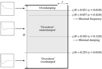
 $$\begin{eqnarray}17\bar{{\it\zeta}}^{2}-20\bar{{\it\zeta}}+4<0\quad \Longrightarrow \quad 0.255<\bar{{\it\zeta}}<0.921.\end{eqnarray}$$
The upper value
 $0.921$
was already found by Kaye & Hunt (Reference Kaye and Hunt2004) from a numerical search aimed at quantifying the critical condition in which a (downward) ‘overshoot’ is possible. These authors used a geometrical parameter
 ${\it\mu}=2{\it\alpha}H/e$
(whose critical value
 ${\it\mu}_{c}$
was
 $0.32$
) related to our parameter
 ${\it\Lambda}$
(
 ${\it\Lambda}=1/{\it\mu}^{2}$
). They also reinterpreted this parameter as being the ratio of two competing time scales (a filling time scale and a draining time scale), which are given for a line plume by
 $T_{f}\sim L/B^{1/3}$
and
 $T_{d}\sim LH/eB^{1/3}$
, respectively. In this light, one can deduce that:
-
(i) for
 $\bar{{\it\zeta}}>0.921$
, draining dominates the process (
$T_{d}\ll T_{f}$
), and the perturbation
${\it\zeta}^{\prime }$
varies as
$+\!\exp (-a{\it\tau})$
(overdamped regime for
${\it\Delta}>0$
) in the vicinity of the horizontal asymptote corresponding to the steady state;
-
(ii) for
$\bar{{\it\zeta}}<0.255$
, filling dominates the process (
$T_{f}\ll T_{d}$
), which creates an initial strong impulse followed by an overdamped regime. In this case, the perturbation
${\it\zeta}^{\prime }$
tends to the (steady-state) horizontal asymptote as
$-\!\exp (-a{\it\tau})$
; -
(iii) for
$0.255<\bar{{\it\zeta}}<0.921$
draining and filling compete, allowing oscillatory behaviour to appear. According to equation (2.9a,b
) (for
${\it\Theta}=0$
,
${\it\alpha}=0.1$
and
$C_{d}=1/\sqrt{2}$
), this corresponds to a top opening width
$e$
ranging from 3 % to 63 % of the box height
$H$
.


Additionally, from relations (3.9) and (3.10) with
 ${\it\Theta}$
set to
 $0$
, it can be shown that the oscillation frequency
 $1/{\it\tau}_{1/2}$
and the damping ratio
 ${\it\beta}$
will be maximal for
 $\bar{{\it\zeta}}=6/7$
and
 $\bar{{\it\zeta}}=6/11$
, respectively. The maximal value that
 ${\it\beta}$
can reach (at
 $\bar{{\it\zeta}}=6/11$
) is
 $0.28\,\%$
. This leads to the conclusion that, for ‘small plumes’, although oscillations can exist, their damping will remain very high. The main results discussed here for ‘small plumes’ are summarized in figure 4.
Main regimes for ‘small plumes’ as a function of the stabilized interface location (the corresponding ratio
 $e/H$
is calculated for
 ${\it\alpha}=0.1$
and for
 $C_{d}\approx 0.7$
).

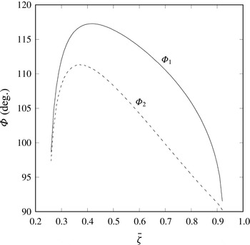
From relation (3.11), in which
 ${\it\Theta}$
is set to 0, figure 5 presents the evolution of the phase shifts
 ${\it\Phi}_{1}$
and
 ${\it\Phi}_{2}$
as a function of the stabilized interface location
 $\bar{{\it\zeta}}$
in the range where oscillations are possible (
 $0.255<\bar{{\it\zeta}}<0.921$
). As expected,
 ${\it\Phi}_{1}$
and
 ${\it\Phi}_{2}$
are minimal and close to
 $90^{\circ }$
at the limits of the oscillating regime. Whatever the value of
 $\bar{{\it\zeta}}$
, the phase shift between
 ${\it\zeta}^{\prime }$
and
 ${\it\eta}^{\prime }$
will always be greater than the one between
 ${\it\zeta}^{\prime }$
and
 ${\it\omega}^{\prime }$
. These conclusions on phase shifts are still valid in the general case (non-‘small plumes’) presented in the next subsection.
Phase shifts
 ${\it\Phi}_{1}$
(between
 ${\it\zeta}^{\prime }$
and
 ${\it\eta}^{\prime }$
) and
 ${\it\Phi}_{2}$
(between
 ${\it\zeta}^{\prime }$
and
 ${\it\omega}^{\prime }$
) as a function of the stabilized interface location
 $\bar{{\it\zeta}}$
for ‘small plumes’.

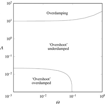
Main regimes in the general case (non-‘small plumes’) as a function of the dimensionless parameter
 ${\it\Theta}$
and the geometrical parameter
 ${\it\Lambda}$
.

3.4. General case – non-‘small plumes’
From relation (2.9a,b
) and inequality (3.8), conditions for which
 ${\it\Delta}<0$
are calculated in the general case (
 ${\it\Theta}\neq 0$
). In the ranges
 $10^{-3}<{\it\Theta}<1$
and
 $10^{-3}<{\it\Lambda}<100$
, the three regimes already mentioned for ‘small plumes’ are shown in figure 6. It can be seen that for
 ${\it\Theta}$
approximately greater than
 $0.1$
, the ‘overshoot’ overdamped regime may disappear, indicating that oscillations are possible provided that the upper layer thickness at steady state
 $h_{ss}$
is greater than
 $H/9$
(i.e.
 $\bar{{\it\zeta}}<8/9$
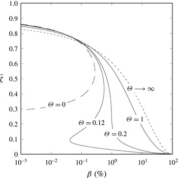
). In order to quantify these oscillations, figure 7 compares the evolution of the damping ratio
 ${\it\beta}$
(in %) as a function of
 $\bar{{\it\zeta}}$
for several values of
 ${\it\Theta}$
including the envelope cases
 ${\it\Theta}=0$
and
 ${\it\Theta}\longrightarrow \infty$
(though an infinite value of
 ${\it\Theta}$
is unrealistic for the applications targeted). Note that these asymptotic cases allow the damping ratio to be expressed analytically as
 $$\begin{eqnarray}\displaystyle {\it\beta}_{({\it\Theta}=0)}=\exp \left[-{\rm\pi}\frac{\bar{{\it\zeta}}+2}{\sqrt{-17\bar{{\it\zeta}}^{2}+20\bar{{\it\zeta}}-4}}\right]\quad \text{and}\quad {\it\beta}_{({\it\Theta}\longrightarrow \infty )}=\exp \left[-{\rm\pi}\sqrt{\bar{{\it\zeta}}/(8/9-\bar{{\it\zeta}})}\right]\!. & & \displaystyle \nonumber\\ \displaystyle & & \displaystyle\end{eqnarray}$$
Figure 7 shows that the damping ratio
 ${\it\beta}$
increases with
 ${\it\Theta}$
for a given value of
 $\bar{{\it\zeta}}$
. For high enough values of
 ${\it\Theta}$
(typically
 ${\it\Theta}\gtrsim 0.2$
),
 ${\it\beta}$
continuously increases when
 $\bar{{\it\zeta}}$
decreases from an upper limit value (that is less than
 $0.921$
but greater than
 $0.889$
) to
 $0$
. From this upper limit value to
 $\bar{{\it\zeta}}\approx 0.7$
, the damping ratio remains very weak and similar to the one obtained for ‘small plumes’. Beyond this value, it can ‘take off’ to reach more significant values as
 $\bar{{\it\zeta}}\longrightarrow 0$
. In this situation, even if the filling process normally dominates the draining process, the interface descends sufficiently to positions where the vertical density gradient in the (non-Boussinesq) plume is strong. The (draining) potential energy of the layer then undergoes marked variations that contribute to reinforcing the oscillations. This conclusion must be qualified, however, by the fact that values of
 $\bar{{\it\zeta}}$
close to
 $0$
are no longer realistic when we consider that, in the present model, the buoyant fluid emerges from a source of finite area. This issue is discussed in the next subsection.
Damping ratio
 ${\it\beta}$
(in %) as a function of
 $\bar{{\it\zeta}}$
for several values of
 ${\it\Theta}$
(axes are reversed for clarity).

3.5. Sources of finite area
For a buoyant fluid emitted (upwards) from a source of finite area (round or 2D), the vertical evolution of the plume variables (velocity
 $u$
, radius or thickness
 $b$
and density
 ${\it\rho}$
) can be exactly and explicitly calculated from a so-called ‘plume function’
 ${\it\Gamma}(z)$
, which quantifies locally the ratio between buoyancy and momentum (see Hunt & Kaye (Reference Hunt and Kaye2005) and Michaux & Vauquelin (Reference Michaux and Vauquelin2008) for extension to non-Boussinesq plumes). Unfortunately,
 ${\it\Gamma}(z)$
is expressed in terms of an incomplete beta function, which limits its usefulness in solving analytically the emptying–filling box problem. Alternatively, and more simply, it is possible to modify self-similar solutions (2.1) by introducing a virtual origin correction (
 $z$
is replaced by
 $z+z_{v}$
where
 $z_{v}$
is the virtual source location). Convenient analytical expressions for the virtual origin location have been offered by Hunt & Kaye (Reference Hunt and Kaye2001) and by Candelier & Vauquelin (Reference Candelier and Vauquelin2012) amongst others. From a mathematical point of view, such a shift is equivalent to considering a line (or point source) plume in a box of height
 $H+z_{v}$
, but with an upper layer thickness that cannot exceed
 $H$
. As a consequence, the domain of variation of
 $\bar{{\it\zeta}}$
is strictly limited between
 $1$
and
 $z_{v}/(H+z_{v})$
, instead of being between
 $1$
and
 $0$
as shown on the ordinate axis in figure 7. For initially buoyancy-dominated plumes (lazy plumes), the virtual origin is expected not to be very far from the actual source, whereas for initially momentum-dominated plumes (forced plumes),
 $z_{v}$
would represent a non-negligible fraction of the box height. This may limit the range of application of the results presented in this article.
4. Conclusions
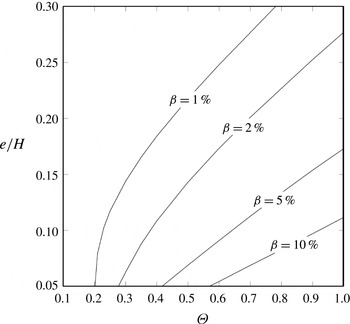
From non-Boussinesq conservation equations, it has been shown that oscillatory behaviour may theoretically occur in the ‘emptying–filling box’ problem (assuming a two-layer displacement ventilation). These oscillations affect not only the thickness of the layer that develops in the box, but also its mean density and the volume flow rate of the (drained) fluid at the top opening. These quantities oscillate with the same period and the same damping ratio but with a phase shift. Oscillations may also exist for Boussinesq plumes but with marked damping. As a practical illustration, figure 8 presents the correspondence (in realistic ranges) between the two key parameters of the problem, the ratio
 $e/H$
and the dimensionless number
 ${\it\Theta}$
, for several fixed values of the damping ratio
 ${\it\beta}$
(in %).
Ratio
 $e/H$
as a function of
 ${\it\Theta}$
for several fixed values of the damping ratio
 ${\it\beta}$
(in %). Calculations consider
 ${\it\alpha}=0.1$
,
 $C_{d}\approx 0.7$
and a line plume model without virtual origin correction.

Appendix A. Extension for (point source) round plumes
In the case of a round non-Boussinesq plume (point source) of buoyancy flux
 $B$
, self-similar solutions for velocity, diameter and density are given by
 $$\begin{eqnarray}u(z)=aB^{1/3}z^{-1/3},\quad d(z)=b\left(\frac{{\it\rho}_{0}}{{\it\rho}}\right)^{1/2}z\quad \text{and}\quad g\frac{{\rm\Delta}{\it\rho}}{{\it\rho}}(z)=cB^{2/3}z^{-5/3},\end{eqnarray}$$
with constants
 $$\begin{eqnarray}a=\frac{1}{2}\left(\frac{25}{6{\rm\pi}{\it\alpha}^{2}}\right)^{1/3},\quad b=\frac{12{\it\alpha}}{5}\quad \text{and}\quad c=\frac{1}{3}\left(\frac{25}{6{\rm\pi}{\it\alpha}^{2}}\right)^{2/3}.\end{eqnarray}$$
Denoting the height and the horizontal surface of the box by
 $H$
and
 $S$
respectively, and the surface of the vent opening by
 ${\it\Sigma}$
, the conservation equations for volume and mass flow rates lead, with the dimensionless variables
 ${\it\zeta}=z/H$
and
 ${\it\eta}={\rm\Delta}{\it\rho}^{\ast }/{\it\rho}^{\ast }$
, to the following equations:
 $$\begin{eqnarray}\displaystyle & \displaystyle \frac{\text{d}{\it\zeta}}{\text{d}{\it\tau}}={\it\omega}{\it\varepsilon}-\frac{{\rm\pi}}{4}ab^{2}{\it\lambda}({\it\zeta}^{5/3}+{\it\Theta}), & \displaystyle\end{eqnarray}$$
 $$\begin{eqnarray}\displaystyle & \displaystyle \frac{\text{d}{\it\eta}}{\text{d}{\it\tau}}=\frac{{\rm\pi}}{4}ab^{2}{\it\lambda}\frac{1+{\it\eta}}{1-{\it\zeta}}({\it\Theta}-{\it\eta}{\it\zeta}^{5/3}). & \displaystyle\end{eqnarray}$$
 $$\begin{eqnarray}{\it\varepsilon}=\frac{{\it\Sigma}}{S},\quad {\it\lambda}=\frac{H^{2}}{S},\quad {\it\omega}=w\frac{H^{1/3}}{B^{1/3}},\quad {\it\tau}=\frac{B^{1/3}}{H^{4/3}}\,t\quad \text{and}\quad {\it\Theta}=\frac{cB^{2/3}}{gH^{5/3}}.\end{eqnarray}$$
The dimensionless number
 ${\it\Theta}$
corresponds to the density deficit in the initial layer at
 $t=0$
, and can also be interpreted as an indicator of the source strength (relative to the local height). With the dimensionless variables defined as before, Bernoulli’s theorem reads
 $$\begin{eqnarray}{\it\omega}^{2}=\frac{2c}{{\it\Theta}}C_{d}^{2}{\it\eta}(1-{\it\zeta}).\end{eqnarray}$$
The dimensionless height
 $\bar{{\it\zeta}}$
where the interface stabilizes is obtained from equations (A 3), (A 4) and (A 6):
 $$\begin{eqnarray}(\bar{{\it\zeta}}^{5/3}+{\it\Theta})^{2}\bar{{\it\zeta}}^{5/3}={\it\Lambda}(1-\bar{{\it\zeta}})\quad \text{with }{\it\Lambda}=\frac{8}{3{\rm\pi}^{2}}\left(\frac{5}{6{\it\alpha}}\right)^{4}\left(\frac{C_{d}{\it\Sigma}}{H^{2}}\right)^{2}.\end{eqnarray}$$
At steady state, the layer density deficit and the dimensionless outflow velocity at the top opening read as
 $$\begin{eqnarray}\bar{{\it\eta}}=\frac{{\it\Theta}}{\bar{{\it\zeta}}^{5/3}}\quad \text{and}\quad \bar{{\it\omega}}=\frac{{\rm\pi}}{4}ab^{2}\frac{{\it\lambda}}{{\it\varepsilon}}(\bar{{\it\zeta}}^{5/3}+{\it\Theta}).\end{eqnarray}$$
The linearization of equations (A 3), (A 4) and (A 6) around the steady-state solution leads to
 $$\begin{eqnarray}\displaystyle & \displaystyle \frac{\text{d}{\it\zeta}^{\prime }}{\text{d}{\it\tau}}=-\frac{5{\rm\pi}}{12}ab^{2}{\it\lambda}\bar{{\it\zeta}}^{2/3}{\it\zeta}^{\prime }+{\it\varepsilon}{\it\omega}^{\prime }, & \displaystyle\end{eqnarray}$$
 $$\begin{eqnarray}\displaystyle & \displaystyle \frac{\text{d}{\it\eta}^{\prime }}{\text{d}{\it\tau}}=-\frac{{\rm\pi}}{4}ab^{2}{\it\lambda}\frac{1+\bar{{\it\eta}}}{1-\bar{{\it\zeta}}}\bar{{\it\zeta}}^{2/3}\left(\frac{5}{3}\bar{{\it\eta}}{\it\zeta}^{\prime }+\bar{{\it\zeta}}{\it\eta}^{\prime }\right), & \displaystyle\end{eqnarray}$$
 $$\begin{eqnarray}\displaystyle & \displaystyle {\it\omega}^{\prime }=-c\frac{C_{d}^{2}}{{\it\Theta}\,\bar{{\it\omega}}}\left[\bar{{\it\eta}}{\it\zeta}^{\prime }-(1-\bar{{\it\zeta}}){\it\eta}^{\prime }\right]. & \displaystyle\end{eqnarray}$$
 ${\it\zeta}^{\prime }$
,
 ${\it\eta}^{\prime }$
and
 ${\it\omega}^{\prime }$
the same second-order differential equation of the form
 $\text{d}^{2}f/\text{d}{\it\tau}^{2}+A_{1}\text{d}f/\text{d}{\it\tau}+A_{2}f=0$
. The coefficients
 $A_{1}$
and
 $A_{2}$
are
 $$\begin{eqnarray}\displaystyle & \displaystyle A_{1}={\rm\pi}ab^{2}{\it\lambda}\left(\frac{5}{12}\bar{{\it\zeta}}^{2/3}+\frac{3}{8}\frac{\bar{{\it\zeta}}^{5/3}+{\it\Theta}}{1-\bar{{\it\zeta}}}\right), & \displaystyle\end{eqnarray}$$
 $$\begin{eqnarray}\displaystyle & \displaystyle A_{2}=\frac{1}{4}({\rm\pi}ab^{2}{\it\lambda})^{2}\frac{\bar{{\it\zeta}}^{5/3}+{\it\Theta}}{1-\bar{{\it\zeta}}}\left[\frac{5}{12}\bar{{\it\zeta}}^{2/3}+\frac{5}{24}\frac{\bar{{\it\zeta}}^{5/3}+{\it\Theta}}{\bar{{\it\zeta}}}+\frac{1}{8}\frac{\bar{{\it\zeta}}^{5/3}+{\it\Theta}}{1-\bar{{\it\zeta}}}\right]. & \displaystyle\end{eqnarray}$$
In the case of ‘small plumes’, namely where
 ${\it\Theta}\approx 0$
, applying the condition
 $A_{1}^{2}<4A_{2}$
to obtain an underdamped regime leads to
 $$\begin{eqnarray}{\textstyle \frac{289}{4}}\bar{{\it\zeta}}^{2}-95\bar{{\it\zeta}}+25<0,\end{eqnarray}$$
which shows that oscillations can exist for
 $0.364<\bar{{\it\zeta}}<0.951$
. The upper value
 $0.951$
corresponds to
 ${\it\Lambda}=15.87$
. We can then formally recover the critical value
 ${\it\mu}_{c}=0.25$
found by Kaye & Hunt (Reference Kaye and Hunt2004) because
 ${\it\Lambda}=1/{\it\mu}^{2}$
.
Using
 $A_{1}$
and
 $A_{2}$
, the main indicators of oscillating regimes (frequency, damping ratio and phase shifts) can be expressed and discussed as functions of the ratio
 ${\it\Sigma}/H^{2}$
and the dimensionless number
 ${\it\Theta}$
.