

1 Introduction
The electrohydrodynamics (EHD) of a drop in a uniform electric field finds relevance in a host of technologically advanced and natural processes. The theoretical model that describes the phenomenon fairly well is the so-called Taylor–Melcher leaky dielectric model (LDM), pioneered by Taylor (Reference Taylor1966) and incisively used by Melcher (Smith & Melcher Reference Smith and Melcher1967; Melcher & Schwarz Reference Melcher and Schwarz1968; Melcher & Smith Reference Melcher and Smith1969; Melcher & Taylor Reference Melcher and Taylor1969) to develop the EHD theory. Briefly, under a weak electric field, the drop elongates in the direction of or perpendicular to the electric field, becoming a prolate or an oblate spheroid, respectively. It can also remain spherical, which is a possibility for leaky dielectric fluids because of intricate interplay of electric and hydrodynamic stresses. The electric field also establishes a circulatory flow in and around the drop, whose direction depends on the relative importance of the electric conductivity ratio  $\widetilde{\unicode[STIX]{x1D70E}}=\unicode[STIX]{x1D70E}_{i}/\unicode[STIX]{x1D70E}_{o}$ (drop fluid/ambient fluid) and the electric permittivity ratio
 $\widetilde{\unicode[STIX]{x1D716}}=\unicode[STIX]{x1D716}_{i}/\unicode[STIX]{x1D716}_{o}$. For
 $\widetilde{\unicode[STIX]{x1D70E}}<\widetilde{\unicode[STIX]{x1D716}}$, the direction of the ambient fluid is from the poles (aligned in the direction of the electric field) to the equator, while for
 $\widetilde{\unicode[STIX]{x1D70E}}>\widetilde{\unicode[STIX]{x1D716}}$ it is the opposite; for
 $\widetilde{\unicode[STIX]{x1D70E}}=\widetilde{\unicode[STIX]{x1D716}}$, the fluid flow ceases to exist, since this is tantamount to a perfect dielectric drop suspended in another perfect dielectric fluid. As the electric field increases, the drop may continue to elongate more or move along a hysteresis curve, where a small increase in the electric field strength at the turning point results in a sudden jump in the deformation. It is also possible that it disintegrates (Zeleny Reference Zeleny1915, Reference Zeleny1917, Reference Zeleny1920; Wilson & Taylor Reference Wilson and Taylor1925; Macky Reference Macky1931; Allan & Mason Reference Allan and Mason1962; Taylor Reference Taylor1964; Torza, Cox & Mason Reference Torza, Cox and Mason1971; Bentenitis & Krause Reference Bentenitis and Krause2005; Lac & Homsy Reference Lac and Homsy2007).
Following the Taylor (Reference Taylor1966) creeping flow solution concerning the steady-state behaviour of a drop in a weak electric field and the Ajayi (Reference Ajayi1978) improvement in the order of accuracy of Taylor’s solution, the theoretical studies have been pursued along different paths to extend the range of validity of the model. Most efforts in this regard have been directed toward determination of the equilibrium shape of the drop at electric field strengths beyond the weak limit (Sherwood Reference Sherwood1988; Tsukada et al. Reference Tsukada, Katayama, Ito and Hozawa1993; Feng & Scott Reference Feng and Scott1996; Lac & Homsy Reference Lac and Homsy2007) while retaining the creeping flow assumption. A few investigators have also looked into the effect of the fluid inertia and convection of charge at the drop surface. Two of the earliest studies in this regard is due to Feng & Scott (Reference Feng and Scott1996) and Feng (Reference Feng1999), respectively. In recent years, the focus has shifted toward exploring the transient dynamics (Dubash & Mestel Reference Dubash and Mestel2007a,Reference Dubash and Mestelb; Esmaeeli & Sharifi Reference Esmaeeli and Sharifi2011; Lanauze, Walker & Khair Reference Lanauze, Walker and Khair2013, Reference Lanauze, Walker and Khair2015; Mandal, Chaudhury & Chakraborty Reference Mandal, Chaudhury and Chakraborty2014; Das & Saintillan Reference Das and Saintillan2017a,Reference Das and Saintillanb). In what follows, we provide a brief account of some of these efforts.
Sherwood (Reference Sherwood1988) was the first to examine the stability of drops in the framework of leaky dielectric theory. He used a boundary integral method and solved the quasi-steady-state creeping flow equations to identify the effect of conductivity ratio on the modes of breakup of prolate drops in several fluid systems. It was shown that highly conducting drops behaved similarly to those in perfectly dielectric fluids, and therefore break up from the tips. On the other hand, in permittivity-matched fluid systems, where the conductivity ratio was the determining factor, a drop more conducting than the surrounding fluid continuously elongated if the conductivity contrast was modest, while it broke up near the tips by dividing into two blobs if the conductivity contrast was sufficiently high. Feng & Scott (Reference Feng and Scott1996) were the first to determine the critical electric field strength  $E_{cr}^{\ast }$ at the turning point for leaky dielectric fluids, who used a Galerkin finite element approach to solve the governing equations. Using an arclength continuation method, they found that, for the drop much more conductive than the surrounding fluid,
 $E_{cr}^{\ast }$ approached that predicted by the electrohydrostatic (EHS) theory regarding a perfectly conducting drop in a perfectly insulating fluid (Garton & Krasucki Reference Garton and Krasucki1964; Taylor Reference Taylor1964; Rosenkilde Reference Rosenkilde1969). The authors also studied the effect of the electric field strength on the steady-state drop deformation under creeping flow regime and showed that in fluid systems for which the drop deformation was vanishingly small, according to the Taylor (Reference Taylor1966) asymptotic results, their computational results recovered the asymptotic ones even at large electric field strengths. Motivated by EHD studies of drops at large electric field strengths (Vizika & Saville Reference Vizika and Saville1992; Tsukada et al. Reference Tsukada, Katayama, Ito and Hozawa1993), Bentenitis & Krause (Reference Bentenitis and Krause2005) extended Taylor’s solution to large deformations using spheroidal coordinates. The authors constructed a map in the physical parameter space, which could be used to predict the two possible behaviours of drops (i.e. continuous elongation versus hysteresis) at strong electric fields but below the critical electric field strength. In a comprehensive study, Lac & Homsy (Reference Lac and Homsy2007) used a boundary integral method and extended the Sherwood (Reference Sherwood1988) analysis to a wide range of dielectric ratios, considering fluid systems of equal viscosity. Building on the second-order solution of Ajayi (Reference Ajayi1978), the authors identified regions where the drop acquired a steady shape, showed hysteresis behaviour or reached a turning point instability past a critical capillary number. They also identified various break-up modes.
Theoretical studies on the transient behaviour of a drop in a weak uniform electric field were initiated by Sozou (Reference Sozou1973), who assumed surface charge build up to be instantaneous and solved the creeping flow equations analytically, while retaining the local fluid acceleration term  $\unicode[STIX]{x2202}\boldsymbol{u}/\unicode[STIX]{x2202}t$. As the focus of this study was on the contribution of the net tangential and normal electric stresses to the evolution of the flow field toward the steady state, the author did not explore deformation-time curve. Furthermore, the solution was not in a closed form. To provide a closed form solution, Esmaeeli & Sharifi (Reference Esmaeeli and Sharifi2011) ignored the local acceleration term and showed that the deformation-time curve was monotonic, with the capillary time scale
 $\unicode[STIX]{x1D707}_{o}a/\unicode[STIX]{x1D6FE}$ being the only characteristic time scale of the problem. Here,
 $\unicode[STIX]{x1D707}_{o}$,
 $a$ and
 $\unicode[STIX]{x1D6FE}$ are the viscosity of the outer fluid, the drop radius and the surface tension, respectively. Lanauze et al. (Reference Lanauze, Walker and Khair2013) accounted for the effect of surface charge relaxation
 $\unicode[STIX]{x2202}q_{s}/\unicode[STIX]{x2202}t$ by extending Sozou’s solution. The authors characterized their results in terms of the Ohnesorge number
 $Oh=(\unicode[STIX]{x1D707}a/\unicode[STIX]{x1D6FE})/(a^{2}/\unicode[STIX]{x1D708})$ and the Saville number
 $Sa=(\unicode[STIX]{x1D716}/\unicode[STIX]{x1D70E})/(a^{2}/\unicode[STIX]{x1D708})$, representing the ratios of the capillary time scale and the charge relaxation time scale to the momentum diffusion time scale, respectively. Here,
 $\unicode[STIX]{x1D716}$,
 $\unicode[STIX]{x1D70E}$ and
 $\unicode[STIX]{x1D708}$ are the electric permittivity, the electric conductivity and the kinematic viscosity, respectively. It was shown that the drop would deform monotonically if charge and momentum relaxation occurred quickly compared to interface deformation,
 $Oh\gg 1$ and
 $Sa\ll 1$ for the droplet and medium. On the other hand, if
 $Sa>1$ or
 $Oh<1$ for either phase, the deformation-time curve would be non-monotonic. It was shown that the droplet and medium behaved as perfect dielectrics at early times, which always favoured an initial prolate deformation.
The effect of charge convection on the transient electrohydrodynamics was studied by Lanauze et al. (Reference Lanauze, Walker and Khair2015) under the creeping flow regime but arbitrary capillary number, using the boundary integral method. Das & Saintillan (Reference Das and Saintillan2017b), on the other hand, studied the problem in the framework of small-deformation theory, where they developed a second-order domain perturbation solution. The authors ignored the  $\unicode[STIX]{x2202}\boldsymbol{u}/\unicode[STIX]{x2202}t$ term but accounted for the surface charge convection
 $\unicode[STIX]{x1D735}_{s}\boldsymbol{\cdot }(\boldsymbol{u}q_{s})$ and relaxation
 $\unicode[STIX]{x2202}q_{s}/\unicode[STIX]{x2202}t$ terms. The picture that emerges from these two studies is that the main effect of charge convection is to reduce the interfacial velocity, leading to oblate drops deforming less but prolate drops deforming more, in agreement with the observations of Feng (Reference Feng1999), who studied the problem numerically in a steady state setting. Transient deformation of a drop in a strong electric field was studied by Zhang, Zahn & Lin (Reference Zhang, Zahn and Lin2013), who extended the steady-state solution of Bentenitis & Krause (Reference Bentenitis and Krause2005) for an ellipsoidal drop, accounting for the charge relaxation
 $\unicode[STIX]{x2202}q_{s}/\unicode[STIX]{x2202}t$. However, they ignored the local acceleration
 $\unicode[STIX]{x2202}\boldsymbol{u}/\unicode[STIX]{x2202}t$ and flow convection
 $\unicode[STIX]{x1D70C}\boldsymbol{u}\boldsymbol{\cdot }\unicode[STIX]{x1D735}\boldsymbol{u}$ as did those authors. Their results were in agreement with those of Dubash & Mestel (Reference Dubash and Mestel2007a), Ha & Yang (Reference Ha and Yang2000) and Bentenitis & Krause (Reference Bentenitis and Krause2005) for the deformation-time curve and steady state deformation, respectively.
Finite Reynolds number computational studies concerning the transient behaviour of the drops have a relatively short history, but are quickly becoming a routine undertaking. The earliest study in this regard is, perhaps, due to Haywood, Renksizbulut & Raithby (Reference Haywood, Renksizbulut and Raithby1991), who used a finite volume method in conjunction with an adaptive grid to study the deformation of drops in liquid/liquid and liquid/gas systems in an axisymmetric setting, treating the fluid systems in both cases as a perfect dielectric. For the range of the Ohnesorge numbers that they considered ( $Oh=2{-}200$) and under a sufficiently small electric field strength (
 $E^{\ast }\ll 1$), the evolution of the drop deformation was monotonic. Supeene, Koch & Bhattacharjee (Reference Supeene, Koch and Bhattacharjee2004) performed simulations using the commercial software package FEMLAB (COMSOL) and studied the transient deformation of a nearly inviscid (
 $\unicode[STIX]{x1D707}=0.001~\text{Pa}~\text{s}$) perfect dielectric liquid drop at low to moderate electric field strengths (
 $3\times 10^{-3}\lessapprox E^{\ast }\lessapprox 0.01$). At all the electric field strengths, the drop settled to its steady state deformation through an oscillatory evolution, where it achieved a large peak that was followed by a much smaller dip and a nearly imperceptible second peak. The deformation-time curves collapsed to a single curve, once the deformation was scaled by the steady-state deformation predicted from the linear theory (O’Konski & Thacher Reference O’Konski and Thacher1953; Allan & Mason Reference Allan and Mason1962) and time was scaled by the natural frequency of oscillation of an inviscid drop. In a follow up article, Supeene, Koch & Bhattacharjee (Reference Supeene, Koch and Bhattacharjee2008) observed a similar behaviour for leaky dielectric systems at low electric field strength.
While the aforementioned studies have significantly enhanced our understanding of the problem, several important issues still remain unanswered. First, the transient behaviour of leaky dielectric drops at finite Reynolds number has not been studied in detail and in an organized way. Thus, little information is available regarding the effect of governing parameters of the problem (such as the fluid system type) on the dynamic response of a drop, and neither a criterion that determines the transition from one dynamic response to the other has been developed, nor is the manner in which the governing parameters affect the time constants of the problem known. Second, there are two misconceptions that have been around for quite some time. One pertains to the relative strength of the hydrodynamic and electric forces in the oblate region of the deformation–circulation map (region I of figure 2), where it is presumed that the drop deforms to an oblate shape because of hydrodynamic forces that are stronger than the electric forces. The other is related to the role of the normal electric stress, where it is assumed that the net normal electric stress always tends to deform a drop to a prolate. Third, the effect of the viscosity ratio on the drop deformation has been studied briefly by Lac & Homsy (Reference Lac and Homsy2007) and Feng & Scott (Reference Feng and Scott1996). However, no justification was provided by these authors regarding their observations. The goal of this study is to shed some light on these issues through numerical simulations and analytical solution.
We use direct numerical simulations to study the problem. The computer code is based on a well-established methodology that has been used in the past to predict the behaviour of a host of multiphase flow problems, in the absence of the electric field (Tryggvason et al. Reference Tryggvason, Bunner, Esmaeeli, Juric, Al-Rawahi, Tauber, Han, Nas and Jan2001). In the context of the electrohydrodynamics of drops, detailed information regarding the mathematical formulation and numerical method can be found in Halim & Esmaeeli (Reference Halim and Esmaeeli2013) and Esmaeeli (Reference Esmaeeli2016). In this study, we solve the governing equations using parallel computing, in conjunction with a message passing interface. The parallel computing algorithm is similar to the one used by Esmaeeli & Tryggvason (Reference Esmaeeli and Tryggvason2005) but has been modified to account for the incorporation of the electric field equations. We consider electric fields of moderate strength, so that the drop will not disintegrate or be subjected to electro-rotation.
The organization of the paper is as follows. In § 2 we discuss the physical set-up and the governing non-dimensional numbers. The background information is provided in § 3, and a brief account of the mathematical formulation and the numerical method are presented in § 4. Section 5 contains the results and discussion. Finally, in § 6 we summarize the new findings.
2 Physical set-up and the governing non-dimensional parameters
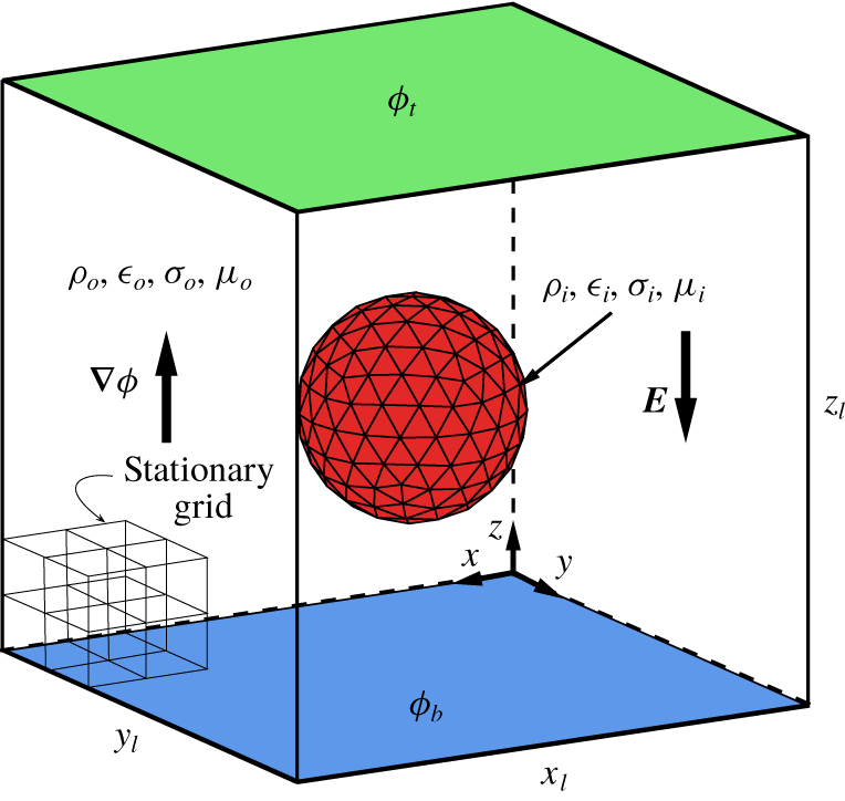
The physical set-up of the problem is shown in figure 1, depicting an initially uncharged liquid drop in a pool of another liquid. Here,  $a$ is the initial radius of the drop, and
 $\unicode[STIX]{x1D70C}$,
 $\unicode[STIX]{x1D707}$,
 $\unicode[STIX]{x1D70E}$,
 $\unicode[STIX]{x1D716}$ and
 $\unicode[STIX]{x1D6FE}$, denote, respectively, the density, the viscosity, the electric conductivity, the electric permittivity and the surface tension. Both fluids are initially quiescent. The electric field is established by assigning uniform electric potentials
 $\unicode[STIX]{x1D719}_{t}$ and
 $\unicode[STIX]{x1D719}_{b}$ to the top and the bottom walls, respectively. Thus, in the absence of the drop, the electric potential is linear (
 $\unicode[STIX]{x1D719}\sim z$) and the electric field strength is uniform, i.e.
 $E_{0}\equiv |\boldsymbol{E}_{0}|=|\unicode[STIX]{x1D719}_{t}-\unicode[STIX]{x1D719}_{b}|/z_{l}$. The computational domain is periodic in the horizontal directions and wall bounded in the vertical direction. No-slip and no-through flow boundary conditions are applied to the velocity field at the walls and periodic boundary conditions are used in the horizontal directions.
The computational set-up, depicting a liquid drop immersed in another liquid. Here  $a$,
 $\unicode[STIX]{x1D70C}$,
 $\unicode[STIX]{x1D707}$,
 $\unicode[STIX]{x1D70E}$ and
 $\unicode[STIX]{x1D716}$ represents, respectively, the radius, the density, the viscosity, the electric conductivity and the electric permittivity. The computational domain is wall bounded in the vertical direction and periodic in the horizontal directions. The moving and the fixed grids are also shown schematically.

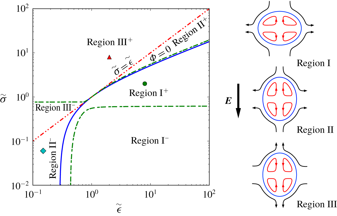
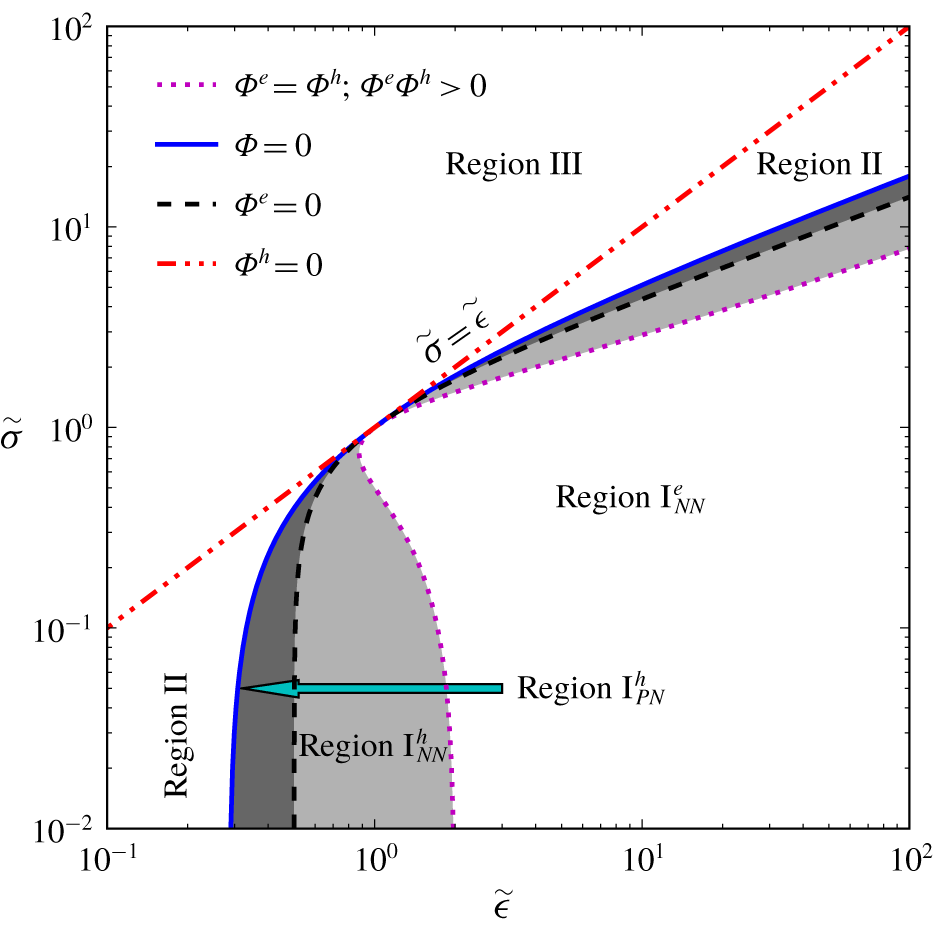
The ‘extended’ deformation–circulation map along with a schematic of the steady-state flow pattern and modes of the drop deformation for  $\widetilde{\unicode[STIX]{x1D707}}=1$. The solid line represents the zero deformation curve, where
 $k_{1}=k_{2}=\unicode[STIX]{x1D6F7}=0$. The dashed-double-dotted line represents the zero-circulation line (
 $\widetilde{\unicode[STIX]{x1D70E}}=\widetilde{\unicode[STIX]{x1D716}}$). The dashed-dotted line shows the
 $k_{1}\neq 0$,
 $k_{2}=0$ line. The ‘
 $+$’ and ‘
 $-$’ superscripts denote the sign of
 $k_{2}$. The coordinates of the fluid systems
 $A{-}C$ are, respectively,
 $\widetilde{\unicode[STIX]{x1D716}}=8$,
 $\widetilde{\unicode[STIX]{x1D70E}}=2$ (circle),
 $\widetilde{\unicode[STIX]{x1D716}}=0.15$,
 $\widetilde{\unicode[STIX]{x1D70E}}=0.06$ (diamond) and
 $\widetilde{\unicode[STIX]{x1D716}}=2$,
 $\widetilde{\unicode[STIX]{x1D70E}}=8$ (triangle).

The governing non-dimensional numbers of the problem can be best identified by non-dimensionalization of the governing equations and their jump conditions. Doing so will put the effect of these terms and their interplay in perspective. Here, it is sufficient to focus on the momentum equation only:
 $$\begin{eqnarray}\unicode[STIX]{x1D70C}_{j}(\unicode[STIX]{x2202}\boldsymbol{u}_{j}/\unicode[STIX]{x2202}t+\boldsymbol{u}_{j}\boldsymbol{\cdot }\unicode[STIX]{x1D735}\boldsymbol{u}_{j})=-\unicode[STIX]{x1D735}p_{j}+\unicode[STIX]{x1D707}_{j}\unicode[STIX]{x1D6FB}^{2}\boldsymbol{u}_{j},\end{eqnarray}$$
where  $j=i,o$ denotes the drop fluid and the ambient fluid, respectively. Considering
 $\unicode[STIX]{x1D70C}_{s}=\unicode[STIX]{x1D70C}_{o}$,
 $\unicode[STIX]{x1D707}_{s}=\unicode[STIX]{x1D707}_{o}$,
 $l_{s}=a$,
 $u_{s}=\unicode[STIX]{x1D716}_{o}E_{0}^{2}a/\unicode[STIX]{x1D707}_{o}$,
 $t_{s}=\unicode[STIX]{x1D707}_{o}a/\unicode[STIX]{x1D6FE}$ and
 $p_{s}=\unicode[STIX]{x1D707}_{o}u_{s}/a\equiv \unicode[STIX]{x1D716}_{o}E_{0}^{2}$ as the density, viscosity, length, velocity, time and pressure scales, and non-dimensionalization of the momentum equation yields
 $$\begin{eqnarray}\unicode[STIX]{x1D70C}_{j}^{\ast }\left(\frac{1}{Oh^{2}}\frac{\unicode[STIX]{x2202}\boldsymbol{u}_{j}^{\ast }}{\unicode[STIX]{x2202}t^{\ast }}+Re_{f}\boldsymbol{u}_{j}^{\ast }\boldsymbol{\cdot }\unicode[STIX]{x1D6FB}^{\ast }\boldsymbol{u}_{j}^{\ast }\right)=-\unicode[STIX]{x1D6FB}^{\ast }p_{j}^{\ast }+\unicode[STIX]{x1D707}_{j}^{\ast }\unicode[STIX]{x1D6FB}^{\ast 2}\boldsymbol{u}_{j}^{\ast }.\end{eqnarray}$$
In (2.1),  $\unicode[STIX]{x1D70C}_{i}^{\ast }=\unicode[STIX]{x1D70C}_{i}/\unicode[STIX]{x1D70C}_{o}\equiv \widetilde{\unicode[STIX]{x1D70C}}$ and
 $\unicode[STIX]{x1D707}_{i}^{\ast }=\unicode[STIX]{x1D707}_{i}/\unicode[STIX]{x1D707}_{o}\equiv \widetilde{\unicode[STIX]{x1D707}}$ are the density and viscosity ratios,
 $Re_{f}=\unicode[STIX]{x1D70C}_{o}au_{s}/\unicode[STIX]{x1D707}_{o}$ is the flow Reynolds number and
 $Oh^{2}=\unicode[STIX]{x1D707}_{o}^{2}/\unicode[STIX]{x1D70C}_{o}a\unicode[STIX]{x1D6FE}$ is the Ohnesorge number squared. Note that
 $\unicode[STIX]{x1D70C}_{o}^{\ast }=1$,
 $\unicode[STIX]{x1D707}_{o}^{\ast }=1$ and
 $u_{s}=\unicode[STIX]{x1D716}_{o}E_{0}^{2}a/\unicode[STIX]{x1D707}_{o}$ is a velocity scale that is constructed by balancing the electric shear stress
 $\unicode[STIX]{x1D749}_{e}\sim \unicode[STIX]{x1D716}_{o}E_{0}^{2}$ and the viscous shear stress
 $\unicode[STIX]{x1D749}_{\unicode[STIX]{x1D707}}\sim \unicode[STIX]{x1D707}_{o}u_{s}/a$ at the surface of the drop.
The momentum equation is supplemented by the shear and normal stress balances at the interface,  $\unicode[STIX]{x27E6}\unicode[STIX]{x1D70F}_{nt}^{e}\unicode[STIX]{x27E7}+\unicode[STIX]{x27E6}\unicode[STIX]{x1D70F}_{nt}^{h}\unicode[STIX]{x27E7}=0$ and
 $\unicode[STIX]{x27E6}\unicode[STIX]{x1D70F}_{nn}^{e}\unicode[STIX]{x27E7}-\unicode[STIX]{x27E6}\,p\unicode[STIX]{x27E7}+\unicode[STIX]{x27E6}\unicode[STIX]{x1D70F}_{nn}^{h}\unicode[STIX]{x27E7}=\unicode[STIX]{x1D705}\unicode[STIX]{x1D6FE}$, respectively. Here, the subscripts
 $t$ and
 $n$ denote the local tangent and normal coordinates at the drop surface, and the superscripts
 $e$ and
 $h$ refer to the electric and hydrodynamic stresses;
 $\unicode[STIX]{x27E6}Q\unicode[STIX]{x27E7}=Q_{o}-Q_{i}$ represents the jump in a typical variable
 $Q$ across the interface, and
 $\unicode[STIX]{x1D705}$ is twice the mean curvature. The structures of
 $\unicode[STIX]{x27E6}\unicode[STIX]{x1D70F}_{nn}^{e}\unicode[STIX]{x27E7}$ and
 $\unicode[STIX]{x27E6}\unicode[STIX]{x1D70F}_{nt}^{e}\unicode[STIX]{x27E7}$ are given in (3.1) and (3.2).
The shear stress balance in non-dimensional form reads
 $$\begin{eqnarray}Ca({\unicode[STIX]{x27E6}\unicode[STIX]{x1D70F}_{nt}^{e}\unicode[STIX]{x27E7}}^{\ast }+{\unicode[STIX]{x27E6}\unicode[STIX]{x1D70F}_{nt}^{h}\unicode[STIX]{x27E7}}^{\ast })=0,\end{eqnarray}$$
where we have used the pressure scale  $p_{s}=\unicode[STIX]{x1D707}_{o}u_{s}/a\equiv \unicode[STIX]{x1D716}_{o}E_{0}^{2}$ to non-dimensionalize the stresses. Here,
 $Ca=\unicode[STIX]{x1D707}_{o}u_{s}/\unicode[STIX]{x1D6FE}$ is the so-called capillary number, which is retained here to emphasize that the net tangential stresses,
 $\unicode[STIX]{x27E6}\unicode[STIX]{x1D70F}_{nt}^{e}\unicode[STIX]{x27E7}$ and
 $\unicode[STIX]{x27E6}\unicode[STIX]{x1D70F}_{nt}^{h}\unicode[STIX]{x27E7}$, are scaled by this number. The appearance of the capillary number in (2.2) can be recognized readily if one notes that the tangential stress balance in general reads
 $\unicode[STIX]{x27E6}\unicode[STIX]{x1D70F}_{nt}^{e}\unicode[STIX]{x27E7}+\unicode[STIX]{x27E6}\unicode[STIX]{x1D70F}_{nt}^{h}\unicode[STIX]{x27E7}=\text{d}\unicode[STIX]{x1D6FE}(s)/\text{d}s$, where the right-hand side represents the surface tension gradient due to the Marangoni effects,
 $s$ being the pertinent arclength of one of the principal curves along the drop surface. Similarly, the non-dimensional normal stress balance reads
 $$\begin{eqnarray}Ca({\unicode[STIX]{x27E6}\unicode[STIX]{x1D70F}_{nn}^{e}\unicode[STIX]{x27E7}}^{\ast }+{\unicode[STIX]{x27E6}\unicode[STIX]{x1D70F}_{nn}^{h}\unicode[STIX]{x27E7}}^{\ast }-\unicode[STIX]{x27E6}\,p\unicode[STIX]{x27E7}^{\ast })=\unicode[STIX]{x1D705}^{\ast },\end{eqnarray}$$
where the terms inside the parentheses have been non-dimensionalized by  $p_{s}=\unicode[STIX]{x1D707}_{o}u_{s}/a\equiv \unicode[STIX]{x1D716}_{o}E_{0}^{2}$, and
 $\unicode[STIX]{x1D705}^{\ast }=\unicode[STIX]{x1D705}a$ is the dimensionless twice-the-mean curvature.
In summary, the governing non-dimensional numbers of the problem are
 $$\begin{eqnarray}\left.\begin{array}{@{}c@{}}Ca={\displaystyle \frac{\unicode[STIX]{x1D707}_{o}u_{s}}{\unicode[STIX]{x1D6FE}}}\equiv {\displaystyle \frac{\unicode[STIX]{x1D716}_{o}E_{0}^{2}a}{\unicode[STIX]{x1D6FE}}},\quad Oh^{2}={\displaystyle \frac{\unicode[STIX]{x1D707}_{o}^{2}}{\unicode[STIX]{x1D70C}_{o}a\unicode[STIX]{x1D6FE}}},\\ \widetilde{\unicode[STIX]{x1D70E}}={\displaystyle \frac{\unicode[STIX]{x1D70E}_{i}}{\unicode[STIX]{x1D70E}_{o}}},\quad \widetilde{\unicode[STIX]{x1D716}}={\displaystyle \frac{\unicode[STIX]{x1D716}_{i}}{\unicode[STIX]{x1D716}_{o}}},\quad \widetilde{\unicode[STIX]{x1D70C}}={\displaystyle \frac{\unicode[STIX]{x1D70C}_{i}}{\unicode[STIX]{x1D70C}_{o}}},\quad \widetilde{\unicode[STIX]{x1D707}}={\displaystyle \frac{\unicode[STIX]{x1D707}_{i}}{\unicode[STIX]{x1D707}_{o}}},\end{array}\right\}\end{eqnarray}$$
noting that  ${\unicode[STIX]{x27E6}\unicode[STIX]{x1D70F}_{nt}^{e}\unicode[STIX]{x27E7}}^{\ast }$ and
 ${\unicode[STIX]{x27E6}\unicode[STIX]{x1D70F}_{nn}^{e}\unicode[STIX]{x27E7}}^{\ast }$ are functions of
 $\widetilde{\unicode[STIX]{x1D70E}}$ and
 $\widetilde{\unicode[STIX]{x1D716}}$ ((3.1), (3.2)). In addition to (2.4), the volume fraction
 $\unicode[STIX]{x1D6FC}=V_{d}/\unicode[STIX]{x1D6FA}$ (
 $V_{d}$ and
 $\unicode[STIX]{x1D6FA}$ being the volume of the drop and the computational domain, respectively) can influence the results if the computational domain is not sufficiently large. Sometimes, in the literature, the non-dimensional electric field strength and the flow Reynolds number
 $$\begin{eqnarray}E^{\ast }=\frac{E_{0}}{\sqrt{\unicode[STIX]{x1D6FE}/\unicode[STIX]{x1D716}_{o}a}}\equiv \sqrt{Ca},\quad Re_{f}=\frac{\unicode[STIX]{x1D70C}_{o}u_{s}a}{\unicode[STIX]{x1D707}_{o}}\end{eqnarray}$$
are used in lieu of  $Ca$ and
 $Oh$, respectively. We note that
 $Re_{f}=Ca/Oh^{2}$.
In addition to the aforementioned governing non-dimensional numbers, we should also refer to two other non-dimensional numbers; namely, the  $Pi$ number
 $\unicode[STIX]{x1D6F1}=\unicode[STIX]{x1D716}\unicode[STIX]{x1D6FE}/\unicode[STIX]{x1D70E}\unicode[STIX]{x1D707}a$ and the electric Reynolds number
 $Re_{el}=\unicode[STIX]{x1D716}a/\unicode[STIX]{x1D70E}u_{s}$. These non-dimensional numbers deal with the relaxation and convection of the surface charge, respectively. Briefly, in typical applications (i.e.
 $\unicode[STIX]{x1D716}=4\unicode[STIX]{x1D716}_{0}~\text{F}~\text{m}^{-1}$,
 $\unicode[STIX]{x1D70E}=10^{-9}~\text{S}~\text{m}^{-1}$,
 $E_{0}=100~\text{kV}~\text{m}^{-1}$,
 $\unicode[STIX]{x1D716}_{0}$ being the permittivity of free space) fluids are electrically neutral on the millimetre length scales and above (Saville Reference Saville1997). Thus, the volume charge conservation equation
 $\unicode[STIX]{x2202}q_{v}/\unicode[STIX]{x2202}t+\unicode[STIX]{x1D735}\boldsymbol{\cdot }(q_{v}\boldsymbol{u}+\unicode[STIX]{x1D70E}\boldsymbol{E})=0$ is simplified to the Laplace equation for the electric potential,
 $\unicode[STIX]{x1D6FB}^{2}\unicode[STIX]{x1D719}=0$. However, this equation needs to be supplemented with the surface charge conservation equation (Saville Reference Saville1997; Castellanos & Gonzalez Reference Castellanos and Gonzalez1998)
 $$\begin{eqnarray}\frac{\unicode[STIX]{x2202}q_{s}}{\unicode[STIX]{x2202}t}+u_{n}\unicode[STIX]{x1D735}\boldsymbol{\cdot }(q_{s}\boldsymbol{n})+\unicode[STIX]{x1D735}_{s}\boldsymbol{\cdot }(\boldsymbol{u}_{s}q_{s})-\left.\unicode[STIX]{x27E6}\unicode[STIX]{x1D70E}\frac{\unicode[STIX]{x2202}\unicode[STIX]{x1D719}}{\unicode[STIX]{x2202}n}\right.\unicode[STIX]{x27E7}=0,\end{eqnarray}$$
where  $u_{n}$ and
 $\boldsymbol{u}_{s}$ are the normal and the tangential components of the fluid velocity at the drop surface,
 $\boldsymbol{n}$ is an outward unit vector normal to the drop surface and
 $\unicode[STIX]{x1D735}_{s}$ is the surface divergence. The terms in (2.6), from the left to the right, account for the charge relaxation, the surface dilation, the charge convection and the charge transport from the bulk due to ohmic conduction, respectively. This equation is made dimensionless, using
 $l_{s}=a$,
 $u_{s}=\unicode[STIX]{x1D716}_{o}E_{0}^{2}a/\unicode[STIX]{x1D707}_{o}$,
 $t_{s}=\unicode[STIX]{x1D707}_{o}a/\unicode[STIX]{x1D6FE}\equiv \unicode[STIX]{x1D70F}_{def}$,
 $Q_{s}=\unicode[STIX]{x1D716}_{o}E_{0}$,
 $\unicode[STIX]{x1D719}_{s}=E_{0}a$ and
 $\unicode[STIX]{x1D70E}_{s}=\unicode[STIX]{x1D70E}_{o}$, as the length, velocity, time, surface charge, electric potential and conductivity scales, leading to
 $$\begin{eqnarray}\unicode[STIX]{x1D6F1}\frac{\unicode[STIX]{x2202}q_{s}^{\ast }}{\unicode[STIX]{x2202}t^{\ast }}+Re_{el}(u_{n}^{\ast }\unicode[STIX]{x1D6FB}^{\ast }\boldsymbol{\cdot }(q_{s}^{\ast }\boldsymbol{n})+\unicode[STIX]{x1D6FB}_{s}^{\ast }\boldsymbol{\cdot }(\boldsymbol{u}_{s}^{\ast }q_{s}^{\ast }))-\left(\frac{\unicode[STIX]{x2202}\unicode[STIX]{x1D719}_{o}^{\ast }}{\unicode[STIX]{x2202}n^{\ast }}-\unicode[STIX]{x1D70E}^{\ast }\frac{\unicode[STIX]{x2202}\unicode[STIX]{x1D719}_{i}^{\ast }}{\unicode[STIX]{x2202}n^{\ast }}\right)=0,\end{eqnarray}$$
where
 $$\begin{eqnarray}\unicode[STIX]{x1D6F1}=\frac{\unicode[STIX]{x1D70F}_{C}}{\unicode[STIX]{x1D70F}_{deff}}\equiv \frac{\unicode[STIX]{x1D716}_{o}/\unicode[STIX]{x1D70E}_{o}}{\unicode[STIX]{x1D707}_{o}a/\unicode[STIX]{x1D6FE}},\quad Re_{el}=\frac{\unicode[STIX]{x1D70F}_{C}}{\unicode[STIX]{x1D70F}_{conv}}\equiv \frac{\unicode[STIX]{x1D716}_{o}/\unicode[STIX]{x1D70E}_{o}}{a/u_{s}}\end{eqnarray}$$
are the  $Pi$ and the electric Reynolds number, respectively. We note that
 $\unicode[STIX]{x1D6F1}=Sa/Oh^{2}$, where
 $Sa=(\unicode[STIX]{x1D716}_{o}/\unicode[STIX]{x1D70E}_{o})/(a^{2}/\unicode[STIX]{x1D708}_{o})\equiv \unicode[STIX]{x1D70F}_{C}/\unicode[STIX]{x1D70F}_{diff}$ is the Saville number.
In (2.8),  $\unicode[STIX]{x1D70F}_{C}=\unicode[STIX]{x1D716}_{o}/\unicode[STIX]{x1D70E}_{o}$ is the time scale of charge relaxation from the bulk to the fluid interface,
 $\unicode[STIX]{x1D70F}_{conv}=a/u_{s}$ is the time scale of charge convection and
 $\unicode[STIX]{x1D70F}_{def}=\unicode[STIX]{x1D707}_{o}a/\unicode[STIX]{x1D6FE}$ is the deformation (or capillary) time scale, during which the drop relaxes to its steady-state deformation. We can safely ignore the charge convection and relaxation in our study, since in the range of physical parameters that we have used,
 $Re_{el}\ll 1$ and
 $\unicode[STIX]{x1D6F1}\ll 1$. Thus, equation (2.7) is simplified to
 $\unicode[STIX]{x27E6}\unicode[STIX]{x1D70E}\unicode[STIX]{x2202}\unicode[STIX]{x1D719}/\unicode[STIX]{x2202}n\unicode[STIX]{x27E7}=0$, which is enforced (implicitly) in our numerical solution (4.1c).
3 Background
The net normal interfacial electric stress
 $$\begin{eqnarray}\unicode[STIX]{x27E6}\unicode[STIX]{x1D70F}_{nn}^{e}\unicode[STIX]{x27E7}=\frac{\unicode[STIX]{x1D716}_{o}}{2}\left[\left(1-\frac{\widetilde{\unicode[STIX]{x1D716}}}{\widetilde{\unicode[STIX]{x1D70E}}^{2}}\right)E_{n_{o}}^{2}+(\widetilde{\unicode[STIX]{x1D70E}}-1)E_{t}^{2}\right]\end{eqnarray}$$
and the net tangential interfacial electric stress
 $$\begin{eqnarray}\unicode[STIX]{x27E6}\unicode[STIX]{x1D70F}_{nt}^{e}\unicode[STIX]{x27E7}=\unicode[STIX]{x1D716}_{o}E_{n_{o}}E_{t}\left(1-\frac{\widetilde{\unicode[STIX]{x1D716}}}{\widetilde{\unicode[STIX]{x1D70E}}}\right)=q_{s}E_{t}\end{eqnarray}$$
are the key parameters that determine, respectively, the sense of drop deformation and fluid circulation in and around the drop. The former is also called the electric pressure. These equations are derived from the Maxwell stress tensor  $\unicode[STIX]{x1D749}_{M}=\unicode[STIX]{x1D716}\boldsymbol{E}\boldsymbol{E}-(1/2)\unicode[STIX]{x1D716}\boldsymbol{I}\boldsymbol{E}\boldsymbol{\cdot }\boldsymbol{E}$, considering tangent-normal coordinates, where
 $\boldsymbol{E}$ and
 $\unicode[STIX]{x1D644}$ are the electric field strength vector and the identity tensor, respectively. In (3.1) and (3.2),
 $E_{t}\equiv E_{t_{i}}=E_{t_{o}}$ and
 $E_{n}$ are the components of
 $\boldsymbol{E}$ in the tangential and normal directions, respectively, and
 $q_{s}=\unicode[STIX]{x1D716}_{o}E_{n_{o}}(1-\widetilde{\unicode[STIX]{x1D716}}/\widetilde{\unicode[STIX]{x1D70E}})$ is the free surface charge. The net tangential interfacial electric stress
 $\unicode[STIX]{x27E6}\unicode[STIX]{x1D70F}_{nt}^{e}\unicode[STIX]{x27E7}$ arises from the action of the tangential component of the electric field at the drop surface
 $E_{t}$ on the surface charge
 $q_{s}$. For a perfectly dielectric drop in a perfectly dielectric liquid,
 $\unicode[STIX]{x27E6}\unicode[STIX]{x1D70F}_{nt}^{e}\unicode[STIX]{x27E7}=0$ since
 $q_{s}=0$. On the other hand, for a perfectly conducting drop in a perfectly dielectric liquid, the electric free charge
 $q_{s}$ is not zero. However,
 $\unicode[STIX]{x27E6}\unicode[STIX]{x1D70F}_{nt}^{e}\unicode[STIX]{x27E7}$ is still zero since
 $E_{t}=0$.
For slightly deformed drops, the deformation is typically characterized by the Taylor deformation parameter (Taylor Reference Taylor1934)
 $$\begin{eqnarray}{\mathcal{D}}=\frac{z_{max}-r_{max}}{z_{max}+r_{max}},\end{eqnarray}$$
where  $z_{max}$ is the maximum end-to-end length in the direction of the electric field and
 $r_{max}$ is the maximum breadth in the transverse direction. Using the Taylor (Reference Taylor1966) solution, Vizika & Saville (Reference Vizika and Saville1992) calculated the steady-state drop deformation for a slight perturbation from sphericity (
 $Ca\ll 1$)
 $$\begin{eqnarray}\displaystyle & {\mathcal{D}}_{\infty }=k_{1}Ca, & \displaystyle\end{eqnarray}$$
 $$\begin{eqnarray}\displaystyle & \displaystyle k_{1}=\frac{9}{16}\frac{\unicode[STIX]{x1D6F7}}{(\widetilde{\unicode[STIX]{x1D70E}}+2)^{2}}, & \displaystyle\end{eqnarray}$$
 $$\begin{eqnarray}\displaystyle & \displaystyle \unicode[STIX]{x1D6F7}=\widetilde{\unicode[STIX]{x1D70E}}^{2}+1-2\widetilde{\unicode[STIX]{x1D716}}+{\displaystyle \frac{3}{5}}(\widetilde{\unicode[STIX]{x1D70E}}-\widetilde{\unicode[STIX]{x1D716}}){\displaystyle \frac{3\widetilde{\unicode[STIX]{x1D707}}+2}{\widetilde{\unicode[STIX]{x1D707}}+1}}, & \displaystyle\end{eqnarray}$$
 $\unicode[STIX]{x1D6F7}$ is the so-called Taylor deformation characteristic function, which determines the sense of drop deformation. For
 $\unicode[STIX]{x1D6F7}<0$, the drop becomes oblate, while for
 $\unicode[STIX]{x1D6F7}>0$ it becomes prolate. For
 $\unicode[STIX]{x1D6F7}=0$ it remains spherical. Taylor’s solution can be treated as a first-order solution in a perturbation series in terms of the capillary number
 $Ca$,
 ${\mathcal{D}}_{\infty }\equiv {\mathcal{D}}^{\langle 1\rangle }=k_{1}Ca$. Ajayi (Reference Ajayi1978) extended it to the second order, which was recast to the following form by Lac & Homsy (Reference Lac and Homsy2007):
 $$\begin{eqnarray}\displaystyle & \displaystyle {\mathcal{D}}_{\infty }^{\langle 2\rangle }=k_{1}Ca+k_{2}Ca^{2}+O(Ca^{3}), & \displaystyle\end{eqnarray}$$
 $$\begin{eqnarray}\displaystyle & \displaystyle k_{2}=\frac{k_{1}}{(\widetilde{\unicode[STIX]{x1D70E}}+2)^{2}}\left[\left(\frac{9}{5}\frac{\widetilde{\unicode[STIX]{x1D70E}}-1}{\widetilde{\unicode[STIX]{x1D70E}}+2}-\frac{1}{16}\right)\unicode[STIX]{x1D6F7}+(\widetilde{\unicode[STIX]{x1D70E}}-\widetilde{\unicode[STIX]{x1D716}})\unicode[STIX]{x1D6FD}(\widetilde{\unicode[STIX]{x1D707}})\right], & \displaystyle\end{eqnarray}$$
 $$\begin{eqnarray}\displaystyle & \displaystyle \unicode[STIX]{x1D6FD}(\widetilde{\unicode[STIX]{x1D707}})=\frac{23}{20}-\frac{139}{210}\left(\frac{1-\widetilde{\unicode[STIX]{x1D707}}}{1+\widetilde{\unicode[STIX]{x1D707}}}\right)-\frac{27}{700}\left(\frac{1-\widetilde{\unicode[STIX]{x1D707}}}{1+\widetilde{\unicode[STIX]{x1D707}}}\right)^{2}. & \displaystyle\end{eqnarray}$$
 $\unicode[STIX]{x1D6F7}$ is a weak function of the viscosity ratio
 $\widetilde{\unicode[STIX]{x1D707}}$, and
 $\unicode[STIX]{x1D6F7}=0$ leads to
 $k_{1}=k_{2}=0$.
The steady-state behaviour of a drop under a weak electric field can be best represented by considering the so-called deformation–circulation map. This map was originally introduced by Torza et al. (Reference Torza, Cox and Mason1971) using the Taylor (Reference Taylor1966) first-order solution, and subsequently extended by Lac & Homsy (Reference Lac and Homsy2007) to account for the Ajayi (Reference Ajayi1978) correction. Figure 2 shows the extended map, which is constructed by plotting  $\unicode[STIX]{x1D6F7}=0$ curve,
 $\widetilde{\unicode[STIX]{x1D70E}}=\widetilde{\unicode[STIX]{x1D716}}$ line and
 $k_{2}=0$ (
 $k_{1}\neq 0$) curve in
 $\widetilde{\unicode[STIX]{x1D70E}}-\widetilde{\unicode[STIX]{x1D716}}$ coordinates. Here, we consider
 $\widetilde{\unicode[STIX]{x1D707}}=1$, since at low electric field strength, the deformation
 ${\mathcal{D}}$ is a weak function of the viscosity ratio
 $\widetilde{\unicode[STIX]{x1D707}}$. The
 $\widetilde{\unicode[STIX]{x1D70E}}=\widetilde{\unicode[STIX]{x1D716}}$ line is called the zero-circulation line, along which the fluid flow ceases to exist at equilibrium, since
 $\widetilde{\unicode[STIX]{x1D70E}}=\widetilde{\unicode[STIX]{x1D716}}$ is tantamount to a perfect dielectric fluid system. The
 $\unicode[STIX]{x1D6F7}=0$ curve is called the zero-deformation curve, along which the drop remains spherical. The
 $\unicode[STIX]{x1D6F7}=0$ curve and the
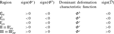
 $\widetilde{\unicode[STIX]{x1D70E}}=\widetilde{\unicode[STIX]{x1D716}}$ line divide the domain into three regions as identified on the map. In region I,
 $\unicode[STIX]{x1D6F7}<0$ and
 $\widetilde{\unicode[STIX]{x1D70E}}<\widetilde{\unicode[STIX]{x1D716}}$, the drop becomes oblate and the external fluid flows from the poles toward the equator. In region II,
 $\unicode[STIX]{x1D6F7}>0$ and
 $\widetilde{\unicode[STIX]{x1D70E}}<\widetilde{\unicode[STIX]{x1D716}}$, the drop becomes prolate and the direction of the external flow remains intact. Finally, in region III,
 $\unicode[STIX]{x1D6F7}>0$ and
 $\widetilde{\unicode[STIX]{x1D70E}}>\widetilde{\unicode[STIX]{x1D716}}$, the drop becomes prolate and the external fluid flows from the equator toward the poles. The inset in the graph schematically depicts the modes of deformation and fluid circulation for each region. When the
 $k_{2}=0$ (
 $k_{1}\neq 0$) curve is added to the map, it divides each region into two subregions, which are identified by adding the superscript (
 $+$) or (
 $-$) to the name of the corresponding region, reflecting the fact that the sign of
 $k_{2}$ is positive or negative in that region.
4 Mathematical formulation and numerical method
The fluids inside and outside the drop, separated by an immiscible phase boundary of constant surface tension, are taken to be incompressible and Newtonian. The material properties are considered to be constant, but not generally equal for each fluid. The governing equations of the problem are conservation of mass and momentum, and the Laplace equation for the electric potential. These equations are valid for each fluid, and are coupled together through jump conditions at the interface. Rather than writing the governing equations separately for each fluid, we use a ‘one-fluid’ formulation, where a single set of equations is used to represent both fluids, and the phase boundary is treated as an embedded interface by adding the appropriate source terms to the conservation laws. These source terms are in the form of delta functions localized at the interface and are selected in such a way to satisfy the correct matching conditions at the phase boundary. The one-fluid equations, governing both fluids, are
 $$\begin{eqnarray}\displaystyle & \displaystyle \unicode[STIX]{x1D70C}\left(\frac{\unicode[STIX]{x2202}\boldsymbol{u}}{\unicode[STIX]{x2202}t}+\unicode[STIX]{x1D735}\boldsymbol{\cdot }(\boldsymbol{u}\boldsymbol{u})\right)=-\unicode[STIX]{x1D735}p+\unicode[STIX]{x1D735}\boldsymbol{\cdot }[\unicode[STIX]{x1D707}(\unicode[STIX]{x1D735}\boldsymbol{u}+(\unicode[STIX]{x1D735}\boldsymbol{u})^{\text{T}})]+\unicode[STIX]{x1D6FE}\int _{S}\unicode[STIX]{x1D705}_{f}\boldsymbol{n}_{f}\unicode[STIX]{x1D6FF}(\boldsymbol{x}-\boldsymbol{x}_{f})\,\text{d}S_{f}+\boldsymbol{F}_{e}, & \displaystyle \nonumber\\ \displaystyle & & \displaystyle\end{eqnarray}$$
 $$\begin{eqnarray}\displaystyle & \displaystyle \unicode[STIX]{x1D735}\boldsymbol{\cdot }\boldsymbol{u}=0, & \displaystyle\end{eqnarray}$$
 $$\begin{eqnarray}\displaystyle & \displaystyle \unicode[STIX]{x1D735}\boldsymbol{\cdot }\unicode[STIX]{x1D70E}\unicode[STIX]{x1D735}\unicode[STIX]{x1D719}=0. & \displaystyle\end{eqnarray}$$
 $\unicode[STIX]{x1D6FE}$ is the surface tension coefficient,
 $\unicode[STIX]{x1D705}$ is the mean curvature,
 $\boldsymbol{n}$ is a normal unit vector at the drop surface pointing toward the drop,
 $\unicode[STIX]{x1D6FF}$ is a three-dimensional delta function and
 $\text{d}S$ is the differential surface area. The variables with subscript
 $f$ are evaluated at the interface;
 $\boldsymbol{x}$ is the point at which the equation is evaluated and
 $\boldsymbol{x}_{f}$ is the position of a point at the interface. The electric force density (
 $\text{N}~\text{m}^{-3}$) is
 $\boldsymbol{F}_{e}=\unicode[STIX]{x1D735}\boldsymbol{\cdot }\unicode[STIX]{x1D749}_{M}$, where
 $\unicode[STIX]{x1D749}_{M}=\unicode[STIX]{x1D716}\boldsymbol{E}\boldsymbol{E}-(1/2)\unicode[STIX]{x1D716}\boldsymbol{I}\boldsymbol{E}\boldsymbol{\cdot }\boldsymbol{E}$ is the Maxwell stress tensor. Equation (4.1b) is formally the same as the conventional mass conservation; however, here the velocity field
 $\boldsymbol{u}$ is defined over the entire domain and changes smoothly from one fluid to the other. Finally, equation (4.1c) should be contrasted with
 $\unicode[STIX]{x1D6FB}^{2}\unicode[STIX]{x1D719}_{i}=\unicode[STIX]{x1D6FB}^{2}\unicode[STIX]{x1D719}_{o}=0$, which is used in the conventional formulation. The fluid properties (
 $\unicode[STIX]{x1D70C}$,
 $\unicode[STIX]{x1D707}$,
 $\unicode[STIX]{x1D70E}$,
 $\unicode[STIX]{x1D716}$) change smoothly from one fluid to the other,
 ${\mathcal{P}}={\mathcal{P}}_{i}H+(1-H){\mathcal{P}}_{o}$, where
 ${\mathcal{P}}$ is a typical property. Here,
 $H(\boldsymbol{x},t)$ is a step function, which is equal to one inside the drop and zero in the outside fluid.
Equation (4.1) enforces the pertinent jump conditions at the interface
 $$\begin{eqnarray}\displaystyle & \unicode[STIX]{x27E6}\unicode[STIX]{x1D749}_{h}-p\boldsymbol{I}\unicode[STIX]{x27E7}\boldsymbol{\cdot }\boldsymbol{n}+\unicode[STIX]{x27E6}\unicode[STIX]{x1D749}_{M}\unicode[STIX]{x27E7}\boldsymbol{\cdot }\boldsymbol{n}=\unicode[STIX]{x1D6FE}\unicode[STIX]{x1D705}\boldsymbol{n}, & \displaystyle\end{eqnarray}$$
 $$\begin{eqnarray}\displaystyle & \unicode[STIX]{x27E6}\boldsymbol{u}\unicode[STIX]{x27E7}\boldsymbol{\cdot }\boldsymbol{n}=0, & \displaystyle\end{eqnarray}$$
 $$\begin{eqnarray}\displaystyle & \unicode[STIX]{x27E6}\boldsymbol{u}\unicode[STIX]{x27E7}\boldsymbol{\cdot }\boldsymbol{t}_{i}=0,\quad i=1,2 & \displaystyle\end{eqnarray}$$
 $$\begin{eqnarray}\displaystyle & \unicode[STIX]{x27E6}\unicode[STIX]{x1D719}\unicode[STIX]{x27E7}=0, & \displaystyle\end{eqnarray}$$
 $$\begin{eqnarray}\displaystyle & \unicode[STIX]{x27E6}\unicode[STIX]{x1D70E}\unicode[STIX]{x1D735}\unicode[STIX]{x1D719}\unicode[STIX]{x27E7}\boldsymbol{\cdot }\boldsymbol{n}=0, & \displaystyle\end{eqnarray}$$
 $\unicode[STIX]{x1D749}_{h}$ is the hydrodynamic stress tensor.
Figure 1 summarizes the computational approach. Here, the drop is represented by triangular elements (Lagrangian grid) and the field variables are computed on a fixed (Eulerian) grid. The computational domain is wall bounded in the vertical direction and periodic in the horizontal directions. The stationary grid is used to discretize the governing equations, and the moving grid marks the position of the phase boundary and is used to keep the stratification of material properties sharp and to calculate the surface tension. This grid is also used to advect the interface by interpolating the velocities of the marker points from the regular grid. The governing equations are solved using parallel computing.
Pertinent information regarding the fluid systems used in this study.

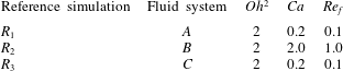
Pertinent information regarding the reference simulations. For all the cases,  $\unicode[STIX]{x1D6FC}=0.035$ and
 $Re_{el}=0.05$.

5 Results
Our aim is to explore transient electrohydrodynamics of a liquid drop in a uniform DC electric field at finite Reynolds number. The governing non-dimensional parameters of the problem are  $Oh^{2}$,
 $Ca$,
 $\unicode[STIX]{x1D6FC}$,
 $\widetilde{\unicode[STIX]{x1D70E}}$,
 $\widetilde{\unicode[STIX]{x1D716}}$,
 $\widetilde{\unicode[STIX]{x1D707}}$ and
 $\widetilde{\unicode[STIX]{x1D70C}}$, as discussed in § 2. Here, we do not examine the effect of
 $\unicode[STIX]{x1D6FC}$ and
 $\widetilde{\unicode[STIX]{x1D70C}}$ on the results, since we are interested in exploring the behaviour of density-matched (
 $\widetilde{\unicode[STIX]{x1D70C}}=1$) ‘solitary’ drops. Thus, for all the simulations performed in this study, the volume fraction is fixed at
 $\unicode[STIX]{x1D6FC}=3.3\,\%$, corresponding to a drop of radius 0.2 unit in a computational box of unit size. Examination of the deformation-time curve of a drop at this volume fraction in a creeping flow regime showed that the steady-state deformation and the associated relaxation time were essentially the same as those for a drop in an unbounded domain (Esmaeeli & Behjatian Reference Esmaeeli and Behjatian2012; Mandal et al. Reference Mandal, Chaudhury and Chakraborty2014).
To examine the effect of dielectric properties ( $\widetilde{\unicode[STIX]{x1D70E}}$ and
 $\widetilde{\unicode[STIX]{x1D716}}$) on the results, it will be more appropriate to choose these two parameters in the context of the so-called deformation–circulation map (figure 2), since it is the relative importance of
 $\widetilde{\unicode[STIX]{x1D70E}}$ and
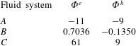
 $\widetilde{\unicode[STIX]{x1D716}}$ that determines the sense of drop deformation and fluid circulation. To this end, we consider three fluid systems as our representative fluid systems. The coordinates of these systems are identified on the map (figure 2) and their dielectric properties are given in table 1. Corresponding to each fluid system, we consider a reference simulation (table 2) as a basis for comparison of the results of the parametric study. To explore the effect of local acceleration
 $\unicode[STIX]{x2202}\boldsymbol{u}/\unicode[STIX]{x2202}t$ on the dynamics, we have chosen
 $Oh^{2}=2$, 0.2 and 0.02, corresponding to
 $Oh^{2}\gg 1$,
 $Oh^{2}\lessapprox 1$ and
 $Oh^{2}\ll 1$, respectively. In selecting
 $Oh^{2}=2$ as the upper limit of the Ohnesorge number we are guided by the fact that the dynamics of the drop will essentially remain the same once
 $Oh>1$. Haywood et al. (Reference Haywood, Renksizbulut and Raithby1991), for example, examined the deformation-time curve of a drop in several perfect dielectric fluid systems for
 $Oh=2$, 20 and 200 using numerical simulations, and observed marginal difference between the deformation-time curve for
 $Oh=2$ and
 $Oh=20$ cases, and the results of the
 $Oh=200$ case were essentially the same as those of the
 $Oh=20$ case. The reference capillary numbers are chosen so that the drop deformation is modest (
 ${\mathcal{D}}\sim 0.1$). Considering the first-order asymptotic solution, equation (3.4), it is seen that the steady-state deformation of the drop is primarily controlled by the characteristic function
 $\unicode[STIX]{x1D6F7}$ and the capillary number
 $Ca=\unicode[STIX]{x1D707}_{o}a/\unicode[STIX]{x1D6FE}$. Here,
 $\unicode[STIX]{x1D6F7}\gg 1$ for fluid systems
 $A$ and
 $C$, while
 $\unicode[STIX]{x1D6F7}<1$ for fluid system
 $B$ (table 1). Thus, an order of magnitude larger capillary number is used for fluid system
 $B$, compared to those of fluid systems
 $A$ and
 $C$, to obtain a deformation that is within the range of those of fluid systems
 $A$ and
 $C$ (table 2). The coordinates of fluid systems
 $A$,
 $B$ and
 $C$ are in subregions
 $\text{I}^{+}$,
 $\text{II}^{-}$ and
 $\text{III}^{+}$; thus, the sign of
 $k_{2}$ is positive for fluid systems
 $A$ and
 $C$, and negative for fluid system
 $B$. Since fluid system
 $A$ is in the oblate region (
 $k_{1}<0$) and fluid systems
 $B$ and
 $C$ are in the prolate regions (
 $k_{1}>0$), the second-order correction leads to
 $|{\mathcal{D}}_{\infty }^{\langle 2\rangle }|<|{\mathcal{D}}_{\infty }^{\langle 1\rangle }|$ for fluid systems
 $A$ and
 $B$, while the opposite holds for fluid system
 $C$. Tables 1–3 summarize the pertinent information about the fluid systems
 $A{-}C$ and reference simulations
 $R_{1}{-}R_{3}$.
Pertinent information regarding the deformation of the drop in the reference simulations,  $R_{1}{-}R_{3}$.

In the computation that follows, we have used a drop of diameter  $d=0.4$ and a cubic computational box of size
 $2.5d$, which is resolved by a
 $128^{3}$ grid. Considering the results of the finest grid as the exact solution, the relative errors in steady-state deformation for
 $32^{3}$,
 $64^{3}$ and
 $128^{3}$ grids were 8.3 %, 1.8 % and 0.34 %, respectively, reflecting the fact that the results are converged for the
 $128^{3}$ grid.
The evolution of the drop and the flow field is controlled by several characteristic times, the relative importance of which can be best understood by representing the governing non-dimensional numbers in terms of the ratios of these characteristic times. This yields
 $$\begin{eqnarray}Oh^{2}=\frac{\unicode[STIX]{x1D70F}_{def}}{\unicode[STIX]{x1D70F}_{diff}}\equiv \frac{\unicode[STIX]{x1D707}_{o}a/\unicode[STIX]{x1D6FE}}{a^{2}/\unicode[STIX]{x1D708}_{o}};\quad Ca=\frac{\unicode[STIX]{x1D70F}_{def}}{\unicode[STIX]{x1D70F}_{conv}}\equiv \frac{\unicode[STIX]{x1D707}_{o}a/\unicode[STIX]{x1D6FE}}{a/u_{s}};\quad Re_{f}=\frac{\unicode[STIX]{x1D70F}_{diff}}{\unicode[STIX]{x1D70F}_{conv}}\equiv \frac{a^{2}/\unicode[STIX]{x1D708}_{o}}{a/u_{s}}.\end{eqnarray}$$
Table 4 presents the relevant time scales of the problem.
The relevant time scales of the problem.

5.1 Dynamic response of a drop
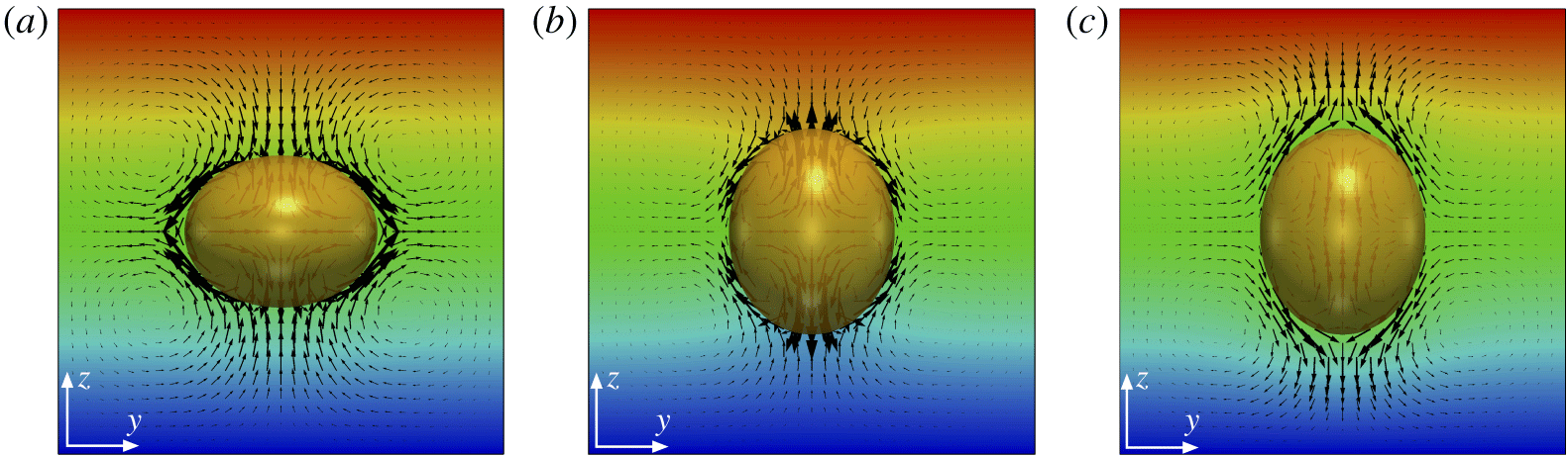
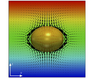
We begin our analysis by considering the evolution of the deformation parameter with time for the reference simulations  $R_{1}{-}R_{3}$. Figure 3 shows the drop, vectors of the velocity field and contours of electric potential field
 $\unicode[STIX]{x1D719}$ in the
 $yz$ midplane at a steady state. The velocity field inside the drop consists of four counter-rotating vortices that are matched with counterpart vortices in the ambient fluid. These vortices are actually the cross-section of toroidal vortices in the midplane. For reference simulations
 $R_{1}$ and
 $R_{2}$, the ambient fluid flows from the poles to the equator, while it runs in the opposite direction for reference simulation
 $R_{3}$. While in an unbounded domain the streamlines in the external flow are open-ended, here they form a closed loop because of the domain confinement.
Vector plot of the velocity field and contours of electric potential  $\unicode[STIX]{x1D719}$ at steady state in the
 $y{-}z$ mid-plane for reference simulations
 $R_{1}{-}R_{3}$ (table 2), corresponding to (a)–(c), respectively.

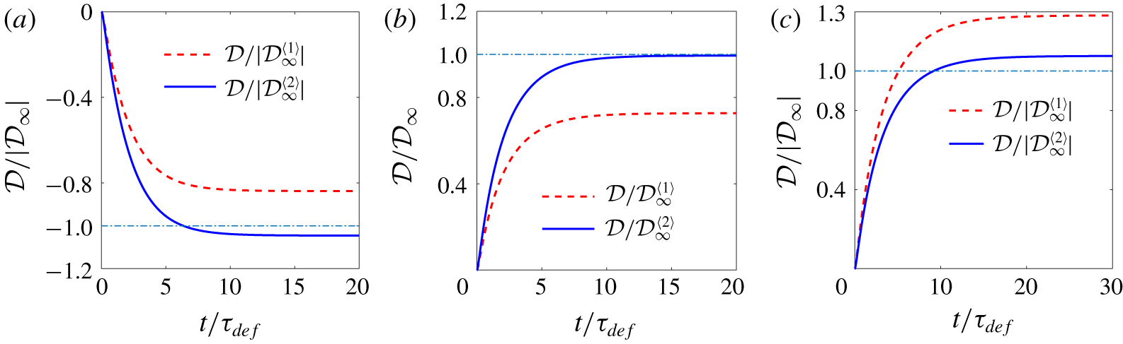
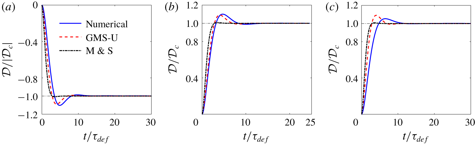
Figure 4 shows the deformation-time curves for the reference simulations. To compare the steady-state deformation with the corresponding creeping flow one, we normalize the deformation parameter by the first- and second-order creeping flow deformations,  ${\mathcal{D}}_{\infty }^{\langle 1\rangle }$ and
 ${\mathcal{D}}_{\infty }^{\langle 2\rangle }$, per (3.4) and (3.5). For these simulations, the steady-state numerical deformation
 $|{\mathcal{D}}_{ss}|$ is approximately 0.1 (table 3). The deformation
 $|{\mathcal{D}}|$ increases monotonically, and as is evident, there is a sizable difference between the numerical and the creeping flow results at the first order; however, the agreements between the two becomes much better at the second order. As expected, the second-order correction reduces the deformation
 $|{\mathcal{D}}|$ for simulations
 $R_{1}$ and
 $R_{2}$, while it increases
 $|{\mathcal{D}}|$ for simulation
 $R_{3}$. Overall, the difference between the numerical deformation and the second-order analytical deformation is minimum for the reference simulation
 $R_{2}$ and maximum for reference simulation
 $R_{3}$. The close agreement between the numerical and the analytical results for simulation
 $R_{2}$ might seem surprising, noting that for this simulation the capillary and flow Reynolds numbers are
 $Ca=2$ and
 $Re_{f}=1$, which deviate substantially from
 $Ca\ll 1$ and
 $Re_{f}\ll 1$ that are the requirements for the validity of the asymptotic solution. This is because the deformation
 ${\mathcal{D}}_{ss}$ is set by not only the capillary number
 $Ca$ but also by the deformation characteristic function
 $\unicode[STIX]{x1D6F7}$, which is quite small for fluid system
 $B$ (table 1). Furthermore, as will be shown in § 5.1.1, the deformation is generally a weak function of the flow Reynolds number
 $Re_{f}$.
Evolution of the normalized deformation  ${\mathcal{D}}/{\mathcal{D}}_{\infty }$ for reference simulations
 $R_{1}{-}R_{3}$ (table 2), corresponding to (a)–(c), respectively.

The results for fluid system  $B$ lend some support to observation of Feng & Scott (Reference Feng and Scott1996), who showed that, for fluid systems for which
 $k_{1}\ll 1$, the drop deformation may be well described by small-deformation theory (Taylor Reference Taylor1966) even at a large strength of the electric field. The authors considered two density- and viscosity-matched fluid systems at
 $\widetilde{\unicode[STIX]{x1D70E}}=0.625$ and
 $\widetilde{\unicode[STIX]{x1D716}}=0.5$ (region II) and
 $\widetilde{\unicode[STIX]{x1D70E}}=1.25$ and
 $\widetilde{\unicode[STIX]{x1D716}}=2$ (region I) in the creeping flow regime, for which
 $k_{1}=0.047$ and
 $-0.1365$, respectively, and showed (their figure 5) that the numerical deformation was essentially the same as the corresponding analytical one for the first fluid system until
 $E^{\ast }=1$, while the difference between the two, for the second fluid system, was very small.
Comparison of the dynamic response of the drop for reference simulations  $R_{1}{-}R_{3}$ (a–c) with the corresponding ones for creeping flow solution.

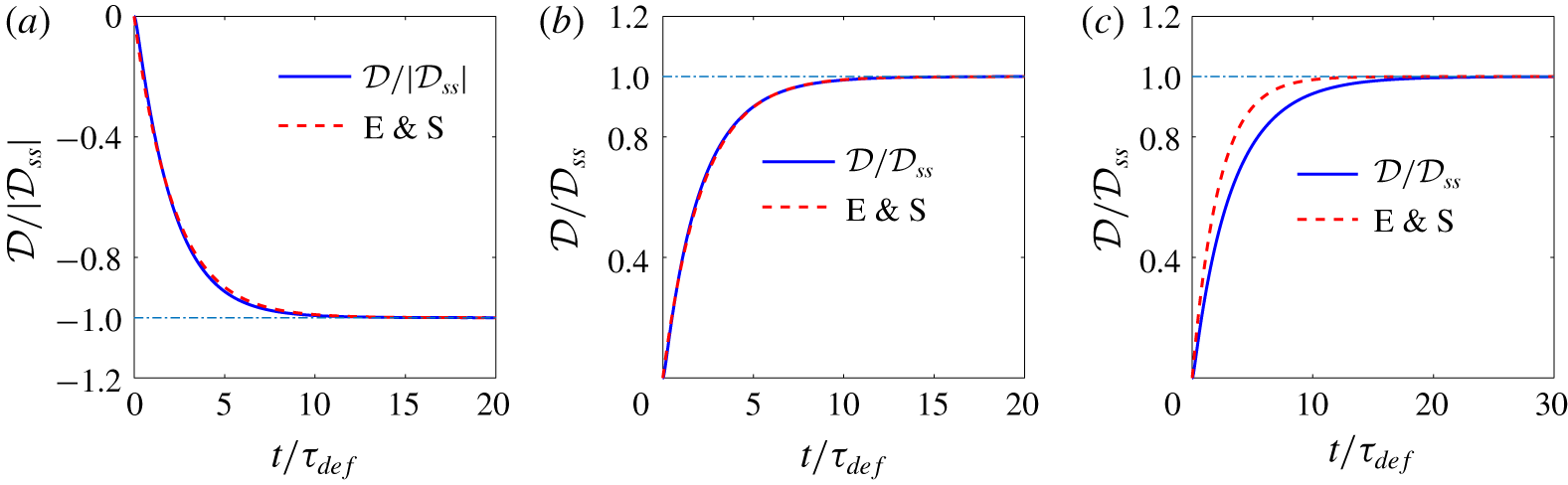
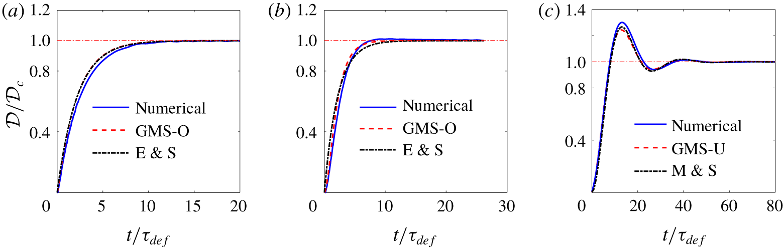
The monotonic evolution of the drop deformation  ${\mathcal{D}}$ with time suggests that the drop dynamics can be modelled as a first-order mechanical system (mass–damper), where the deformation
 ${\mathcal{D}}$ is essentially controlled by a capillary time scale
 $\unicode[STIX]{x1D707}a/\unicode[STIX]{x1D6FE}$. To explore this idea, in figure 5 we compare the evolution of the drop deformation (normalized by its steady-state deformation) with that predicted by the creeping flow analytical solution (Esmaeeli & Sharifi Reference Esmaeeli and Sharifi2011):
 $$\begin{eqnarray}\displaystyle & \displaystyle {\mathcal{D}}/{\mathcal{D}}_{\infty }=1-\exp (-t/\unicode[STIX]{x1D70F}), & \displaystyle\end{eqnarray}$$
 $$\begin{eqnarray}\displaystyle & \displaystyle \unicode[STIX]{x1D70F}=\frac{\unicode[STIX]{x1D707}_{o}a}{\unicode[STIX]{x1D6FE}}\frac{(19\widetilde{\unicode[STIX]{x1D707}}+16)(2\widetilde{\unicode[STIX]{x1D707}}+3)}{40(\widetilde{\unicode[STIX]{x1D707}}+1)}. & \displaystyle\end{eqnarray}$$
 $Oh^{2}\gg 1$,
 $Re_{f}\ll 1$,
 $Ca\ll 1$ and
 $\unicode[STIX]{x1D6F1}\ll 1$. Because of the normalization of (5.2), it is inconsequential if
 ${\mathcal{D}}_{\infty }^{\langle 1\rangle }$ or
 ${\mathcal{D}}_{\infty }^{\langle 2\rangle }$ is used to represent
 ${\mathcal{D}}_{\infty }$. For reference simulations
 $R_{1}$ and
 $R_{2}$, the agreements between the numerical and the analytical relaxation times are close, implying that the dynamic response is essentially the same as that in a creeping flow. On the other hand, for reference simulation
 $R_{3}$, the difference in the relaxation times is more pronounced. We believe the discrepancy is due to the dependency of the relaxation time on the ratio of the dielectric properties (
 $\widetilde{\unicode[STIX]{x1D70E}}$,
 $\widetilde{\unicode[STIX]{x1D716}}$) and the capillary number
 $Ca$, which affect the numerical results, but are not accounted for in the analytical solution. This issue will be discussed in § 5.1.5.
5.1.1 Effect of the  $Oh^{2}$ number

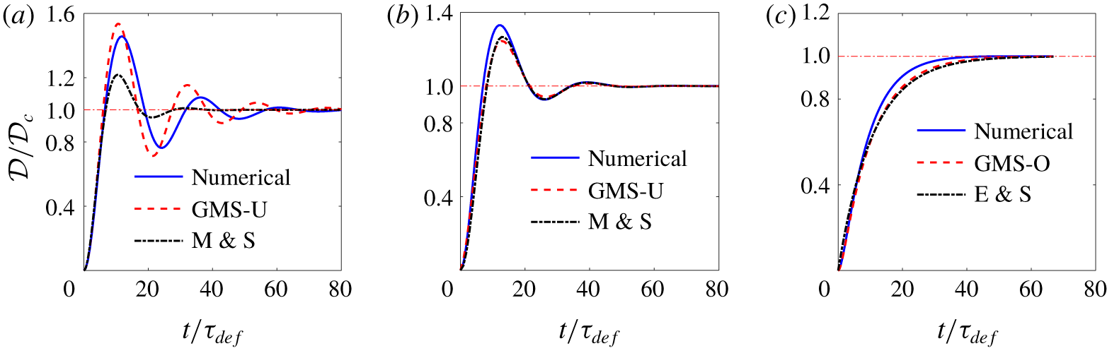
The monotonic behaviour seen in figures 4 and 5 for the deformation-time curves will be disrupted if  $Oh^{2}$ becomes sufficiently small. This parameter controls the response dynamics through the local acceleration term
 $\unicode[STIX]{x2202}\boldsymbol{u}/\unicode[STIX]{x2202}t$, per (2.1). For the ambient fluid,
 $1/Oh^{2}$ emerges as the parameter that controls the local acceleration term. However, considering this equation for the drop fluid and balancing the first and last terms suggests that
 $$\begin{eqnarray}\frac{\widetilde{\unicode[STIX]{x1D70C}}}{\widetilde{\unicode[STIX]{x1D707}}}\left(\frac{1}{Oh^{2}}\right)\end{eqnarray}$$
is the parameter that controls the local acceleration in general. Thus, small  $Oh^{2}$, as well as large
 $\widetilde{\unicode[STIX]{x1D70C}}$ and small
 $\widetilde{\unicode[STIX]{x1D707}}$, favours an oscillatory behaviour. Generally speaking, smaller
 $Oh^{2}$ number is tantamount to a larger drop or a less viscous surroundings.
To explore the effect of variation of  $Oh^{2}$ on the deformation-time curve, we have performed two other simulations at
 $Oh^{2}=0.2$ and 0.02 to compare with the reference simulation,
 $Oh^{2}=2$. Since in these simulations the capillary number
 $Ca$ is fixed, a smaller
 $Oh^{2}$ leads to a larger flow Reynolds number
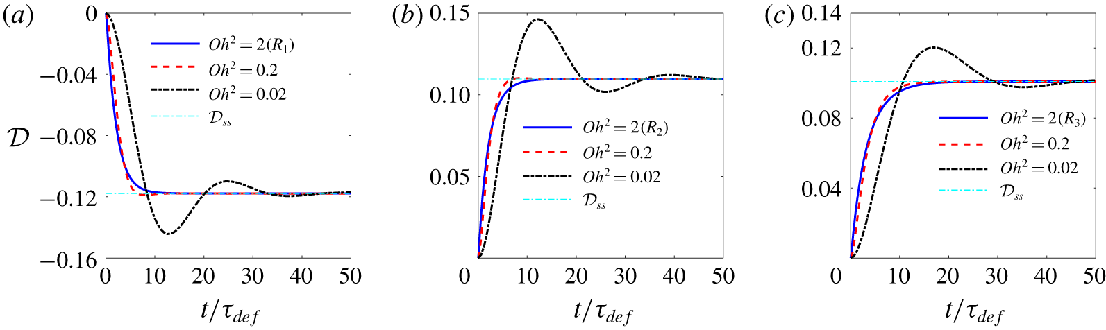
 $Re_{f}=Ca/Oh^{2}$. Figure 6 compares the effect of
 $Oh^{2}$ on the deformation-time history for fluid systems
 $A{-}C$. As is evident, the dynamic response transitions from a monotonic response to an oscillatory one as
 $Oh^{2}$ decreases from 2 to 0.02. For
 $Oh^{2}=2$, the dynamic response is overdamped for all the simulations. For
 $Oh^{2}=0.2$ it is slightly underdamped for fluid system
 $A$ as the deformation
 $|{\mathcal{D}}(t)|$ exceeds the steady-state deformation
 $|{\mathcal{D}}_{ss}|$ at some time, while it is overdamped for fluid systems
 $B$ and
 $C$. However, inspection of the deformation-time curves showed the existence of an inflection point during the transient period for these two fluid systems. This suggests that the dynamic response for all the three fluid systems at
 $Oh^{2}=0.2$ is controlled by more than one time scale. For
 $Oh^{2}=0.02$, the dynamic response resembles that of an underdamped second-order mechanical system, where the drop settles to its steady state via an oscillatory motion. Here, the deformation has a large initial peak that is followed by a smaller dip, and nearly an imperceptible second peak. The overshoot is the largest for fluid system
 $B$ and is nearly the same for fluid systems
 $A$ and
 $C$. This is plausible since flow Reynolds number
 $Re_{f}$ for fluid system
 $B$ is 100, while it is 10 for the other two fluid systems.
Comparison of deformation-time history as a function of  $Oh^{2}$ for fluid systems
 $A{-}C$, corresponding to (a)–(c), respectively. The
 $Oh^{2}=2$ curves correspond, respectively, to
 $R_{1}{-}R_{3}$ reference simulations (table 2). For all the cases
 $\widetilde{\unicode[STIX]{x1D70C}}=1$ and
 $\widetilde{\unicode[STIX]{x1D707}}=1$.

Two observations can be made here. First, the steady-state deformation for each set of simulations (fluid system) is essentially independent of  $Oh^{2}$, and hence
 $Re_{f}$, which characterizes the fluid inertia. This is evident from figure 6, where the steady-state deformation remains nearly the same over two orders of magnitude variation in the flow Reynolds number, i.e.
 $Re_{f}=0.1,1,10$ for fluid systems
 $A$ and
 $C$, and
 $Re_{f}=1,10,100$ for fluid system
 $B$. Second, the reason for the appearance of the first peak in the
 $Oh^{2}=0.02$ simulations is that the deformation settles to a steady state corresponding to the time scale of deformation
 $\unicode[STIX]{x1D70F}_{def}=\unicode[STIX]{x1D707}_{o}a/\unicode[STIX]{x1D6FE}$. However, since in the long term the dynamics is controlled by the momentum diffusion time scale
 $\unicode[STIX]{x1D70F}_{diff}$ (recall
 $Oh^{2}=\unicode[STIX]{x1D70F}_{def}/\unicode[STIX]{x1D70F}_{diff}$), the drop settles to its final steady state over a time that is dictated by this time scale. The oscillation period for the
 $Oh^{2}\ll 1$ simulations is estimated from the inviscid theory to be
 $\unicode[STIX]{x1D70F}_{\unicode[STIX]{x1D714}}=\sqrt{\unicode[STIX]{x1D70C}_{o}a^{3}/\unicode[STIX]{x1D6FE}}$. This time scale can be rewritten as
 $\unicode[STIX]{x1D70F}_{\unicode[STIX]{x1D714}}=\sqrt{\unicode[STIX]{x1D70F}_{def}\unicode[STIX]{x1D70F}_{diff}}$, which asserts that
 $\unicode[STIX]{x1D70F}_{def}<\unicode[STIX]{x1D70F}_{\unicode[STIX]{x1D714}}<\unicode[STIX]{x1D70F}_{diff}$ for
 $Oh^{2}<1$.
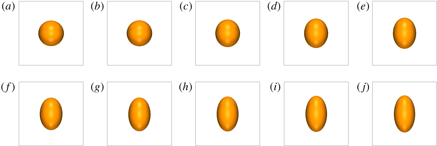
Steady-state drop shape for fluid system  $A$ at
 $Oh^{2}=0.02$. The capillary numbers are 0.02, 0.2, 0.35, 0.6, 0.75, 1, 1.5 and 2, corresponding to (a)–(h).

5.1.2 Effect of the $Ca$ number

The capillary number  $Ca$ controls the drop behaviour through the net normal and shear stresses, per (2.2) and (2.3). We study the effect of this parameter on the dynamic response of the drop by performing a few simulations over three orders of magnitude of the capillary number at
 $Oh^{2}=2$, 0.2 and 0.02. The effect of the capillary number on the equilibrium shape and stability of the drops has been reasonably well studied (Sherwood Reference Sherwood1988; Feng & Scott Reference Feng and Scott1996; Lac & Homsy Reference Lac and Homsy2007). However, not much is known about the impact of this parameter on the transient behaviour of the drops. Here, the literature is limited to only a few studies. For weak electric field strength (
 $E^{\ast }\ll 1$), Supeene et al. (Reference Supeene, Koch and Bhattacharjee2004) studied the deformation of a drop in a perfectly dielectric and nearly inviscid (
 $Oh^{2}\ll 1$) fluid system at several imposed electric field strengths and showed that the normalized dynamic response (
 ${\mathcal{D}}/{\mathcal{D}}_{\infty }$ versus
 $t/\unicode[STIX]{x1D70F}_{\unicode[STIX]{x1D714}}$), which was oscillatory, collapsed to a single curve,
 ${\mathcal{D}}_{\infty }$ being the steady-state deformation of a perfectly dielectric drop in a weak electric field (O’Konski & Thacher Reference O’Konski and Thacher1953; Allan & Mason Reference Allan and Mason1962). For intermediate (
 $E^{\ast }<E_{cr}^{\ast }$) and large (
 $E^{\ast }>E_{cr}^{\ast }$) electric field strengths, Zhang et al. (Reference Zhang, Zahn and Lin2013) performed a semi-numerical study, where they ignored the local acceleration term, but allowed for the surface charge relaxation. For the former, the drop deformed monotonically and settled to a steady-state deformation. For the latter, the deformation proceeded monotonically and slowly in time until it reached a plateau, where the deformation suddenly increased, at which point the drop became unstable.
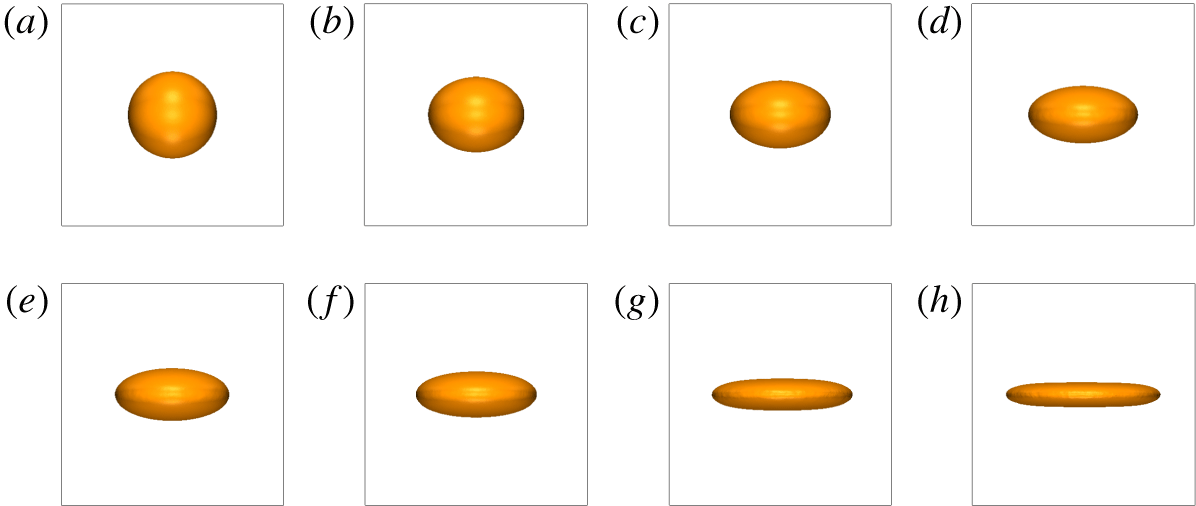
Figure 7 shows the steady-state drop shapes for fluid system  $A$ at
 $Oh^{2}=0.02$, spread over three orders of magnitude of capillary number (
 $Ca=0.02{-}2$). Here, the drop elongates in the direction perpendicular to the field. As the capillary number increases, the drop shape evolves from a spheroid to an ellipsoid, and eventually a donut shape. For this fluid system and in an unbounded domain, the drop would remain stable for all the capillary numbers, according to the Ajayi (Reference Ajayi1978) second-order creeping flow solution, i.e.
 $k_{1}k_{2}<0$. For the finite computational domain used here, the drop will be eventually influenced by the drops in the adjacent periodic cells beyond a capillary number.
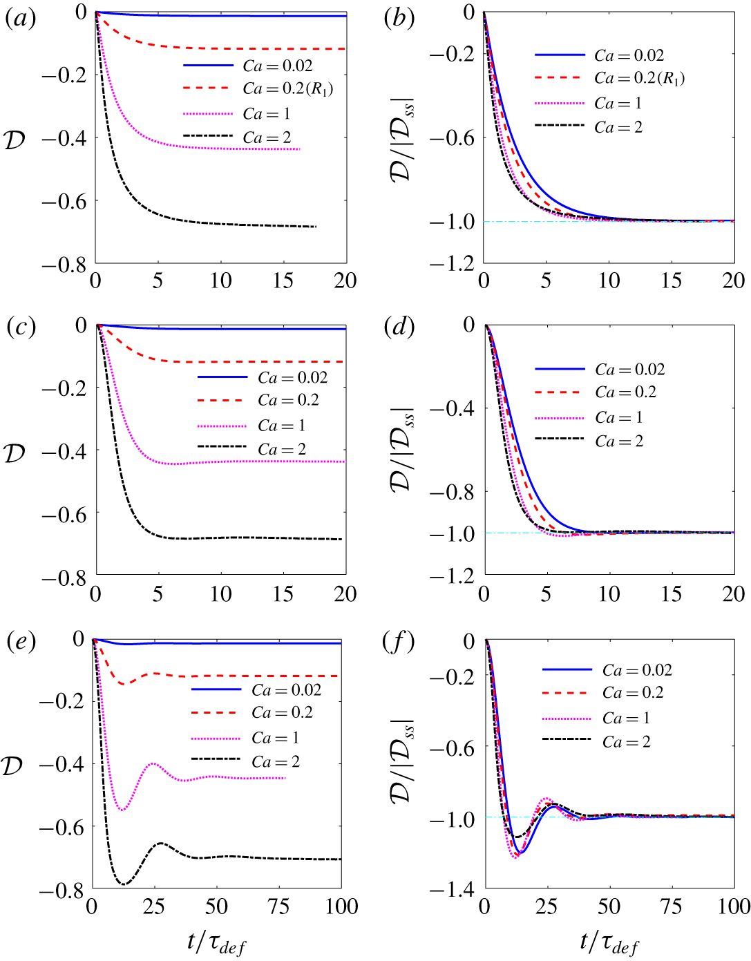
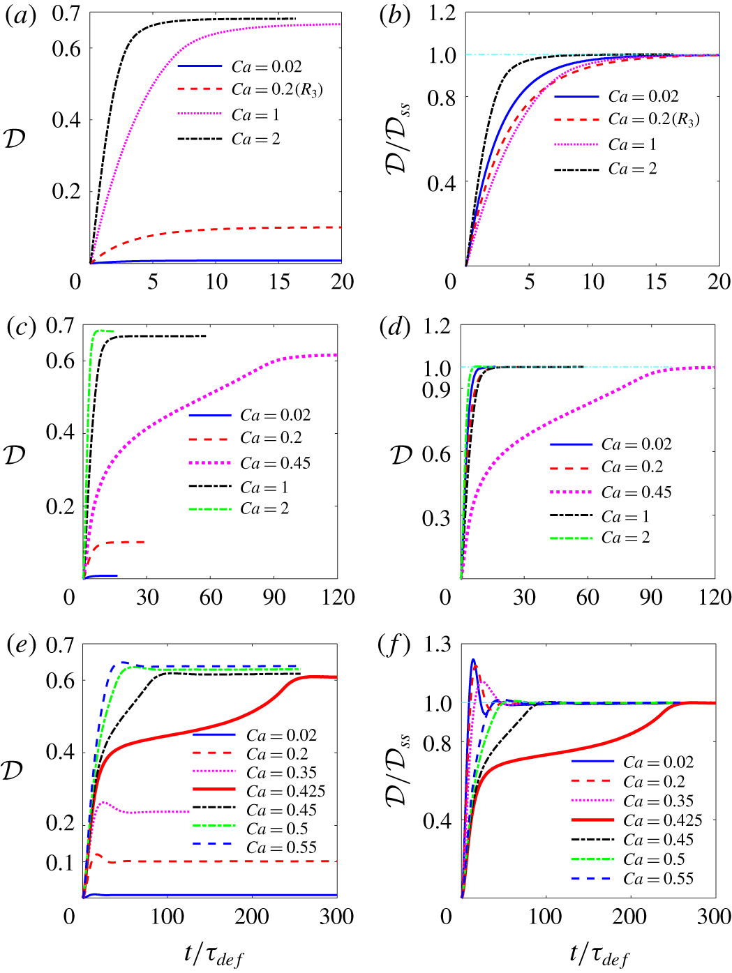
Figure 8 shows the deformation-time curves for representative simulations. The unscaled deformation parameter  ${\mathcal{D}}$ (a,c,e) highlights the effect of the capillary number on the degree of the deformation and the initial rate of the deformation
 $\unicode[STIX]{x2202}{\mathcal{D}}/\unicode[STIX]{x2202}t|_{t=0}$, and the normalized deformation
 ${\mathcal{D}}/{\mathcal{D}}_{ss}$ (b,d,f;
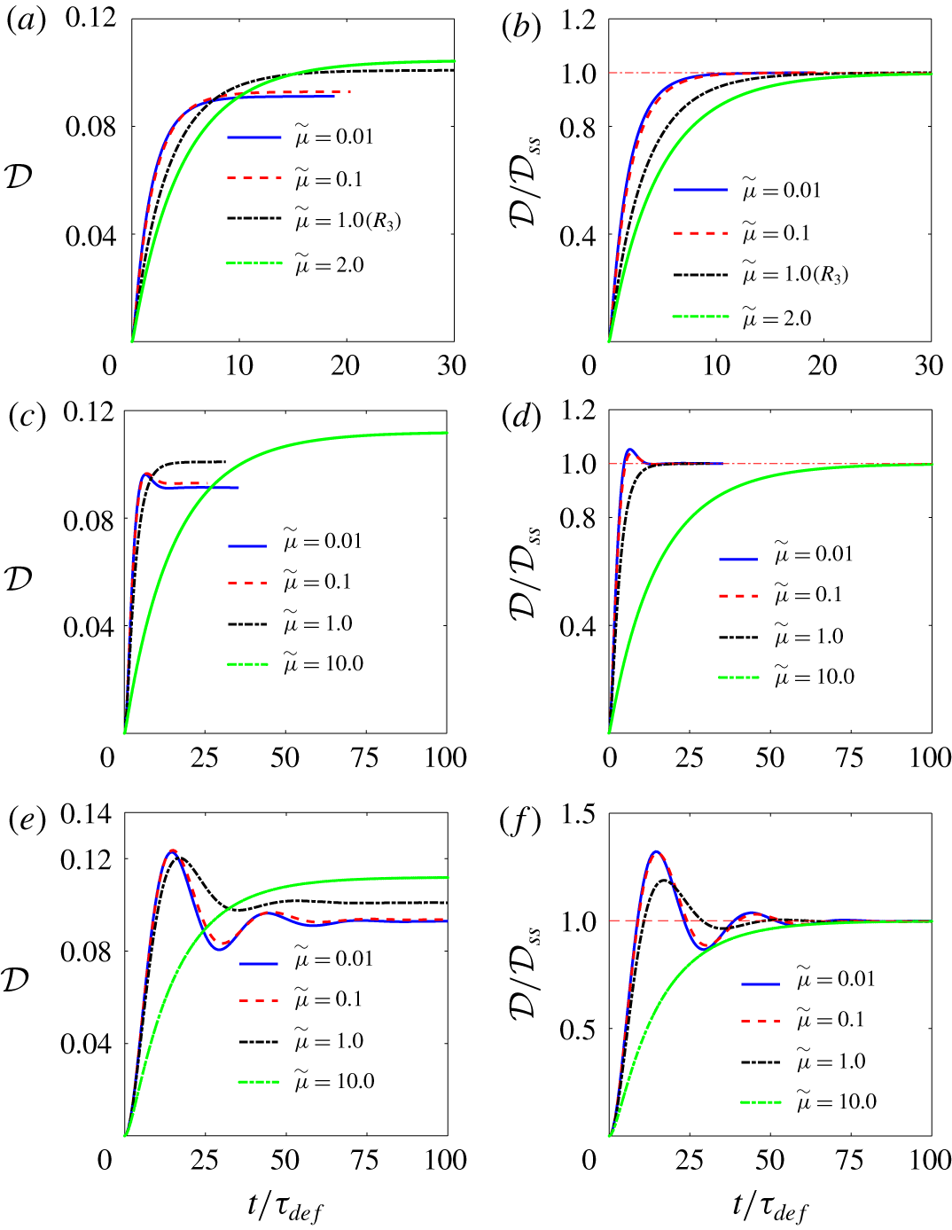
 ${\mathcal{D}}_{ss}$ being the steady-state deformation) provides the possibility of comparison of the dynamic response with that of a linear system (mass–damper or mass–damper–spring). Considering the left panels, the dynamic response gradually transitions from a monotonic response to an oscillatory one with a decrease in the
 $Oh^{2}$ number. For the monotonic evolution (a,c), the time constant at which the drop settles to its steady-state deformation decreases with an increase in the capillary number. Similarly, for the oscillatory evolution (e), the increase in the capillary number results in a decrease in the time at which the deformation reaches its first peak. These observations are in accord with intuition and are in line with the non-dimensionalization of the governing equations; as the capillary number increases, the electric pressure increases (per (2.3)) and, therefore, the drop deforms faster.
Evolution of deformation parameter with time at different capillary numbers for fluid system  $A$ for
 $Oh^{2}=2$, 0.2 and 0.02, corresponding to (a,b), (c,d) and (e,f), respectively. Here,
 $R_{1}$ in (a,b) denotes the reference simulation. For all the cases,
 $\widetilde{\unicode[STIX]{x1D70C}}=1$ and
 $\widetilde{\unicode[STIX]{x1D707}}=1$.

For  $Oh^{2}=2$, the result of the reference simulation
 $R_{1}$, figure 5(a), is identified on the figure. Here, the dynamic response resembles that of a first-order mechanical system,
 ${\mathcal{D}}={\mathcal{D}}_{ss}[1-\exp (-t/\unicode[STIX]{x1D70F}_{rel})]$, where
 $\unicode[STIX]{x1D70F}_{rel}$ is the relaxation time (b). The dependency of the relaxation time
 $\unicode[STIX]{x1D70F}_{rel}$ on the input parameters of the problem is discussed in § 5.1.5. For
 $Oh^{2}=0.2$, the dynamic response is overdamped for
 $Ca=0.02$, becomes slightly underdamped for
 $Ca=0.2$ and 1 and switches back to an overdamped response at
 $Ca=2$ (d). Here, the dynamic response is controlled by more than one time scale as the inspection of the
 ${\mathcal{D}}-t$ curves through magnification (not shown here) showed the appearance of an inflection point during the transient period. As such, the dynamic response at
 $Oh^{2}=0.2$ and low capillary number
 $Ca\ll 1$ seems to be well represented by that of a second-order mechanical system. For
 $Oh^{2}=0.02$, the dynamic response is underdamped for all the capillary numbers (f). Here, the normalized peak increases with an increase in the capillary number for
 $Ca\leqslant 1$ but it decreases for
 $Ca=2$. We believe the change in the behaviour of the curves for
 $Ca>1$ in these simulations is due to the deviation of the drop shape from the ellipsoidal shape. This point will be elucidated in § 5.1.5.
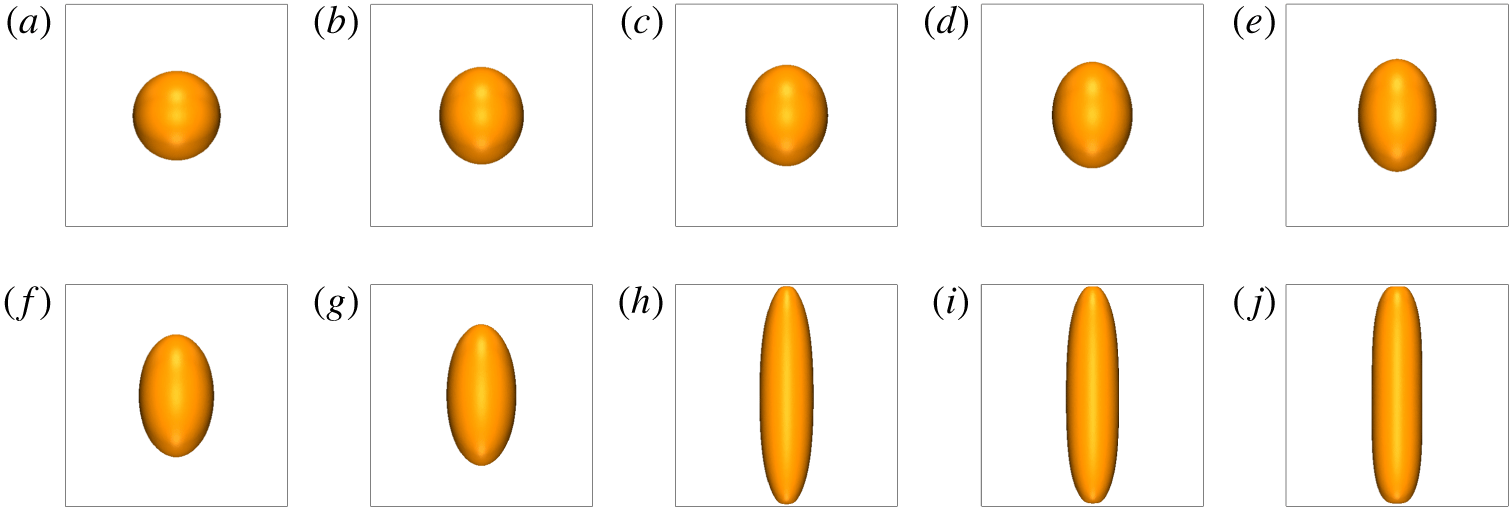
Figure 9 shows the steady-state drop shape for fluid system  $B$ at
 $Oh^{2}=0.02$, spread over three orders of magnitude of the capillary number (
 $Ca=0.02{-}8$). Here, the drop deforms to a prolate and the change in the degree of the deformation with the capillary number is rather slow because the characteristic deformation function
 $\unicode[STIX]{x1D6F7}$ is low (table 1). For this fluid system and in an unbounded domain, the drop would remain stable for all capillary numbers, according to the Ajayi (Reference Ajayi1978) second-order creeping flow solution, i.e.
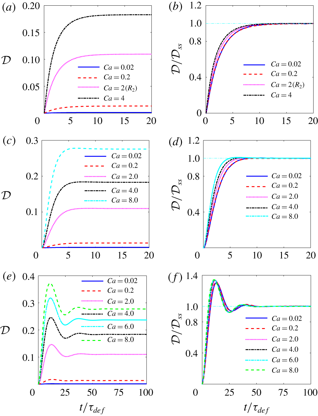
 $k_{1}k_{2}<0$. However, for the finite computational domain used here, the elongation of the drop will eventually be limited by the size of the computational box in the vertical direction beyond a certain capillary number. Figure 10 shows the deformation-time curves for a few representative simulations pertaining to this fluid system. For
 $Oh^{2}=2$, the result of the reference simulation
 $R_{2}$, figure 5(b), is identified on the figure. The drop deforms monotonically for both
 $Oh^{2}=2$ and 0.2, and becomes oscillatory for
 $Oh^{2}=0.02$. The normalized deformation curves are nearly indistinguishable from one another for
 $Ca=0.02{-}0.2$ for each set of curves. For
 $Oh^{2}=0.02$, in particular, the normalized curves are essentially the same over the entire range of capillary number (
 $Ca=0.02{-}8$). As in fluid system
 $A$, the time constant for the monotonic (a–d) and the oscillatory (e,f) evolutions correlates positively with the capillary number.
Steady-state drop shape for fluid system  $B$ at
 $Oh^{2}=0.02$. The capillary numbers are 0.02, 0.2, 1, 2, 3, 4, 5, 6, 7 and 8, corresponding to (a)–(j).

Evolution of deformation parameter with time at different capillary numbers for fluid system  $B$ for
 $Oh^{2}=2$, 0.2 and 0.02, corresponding to (a,b), (c,d) and (e,f), respectively. Here,
 $R_{2}$ in (a,b) denotes the reference simulation. For all the cases,
 $\widetilde{\unicode[STIX]{x1D70C}}=1$ and
 $\widetilde{\unicode[STIX]{x1D707}}=1$.

Figure 11 shows the steady-state drop shape for fluid system  $C$ at
 $Oh^{2}=0.02$, spread over three orders of magnitude of capillary number (
 $Ca=0.02{-}0.55$). For this fluid system and in an unbounded domain, the drop could become unstable beyond a critical capillary number, according to the Ajayi (Reference Ajayi1978) second-order creeping flow solution; i.e.
 $k_{1}k_{2}>0$. As in fluid system
 $B$, the drop deforms to a prolate. However, there are two main differences between the evolution of the drops in the two fluid systems. First, here, the rate of the deformation with the capillary number
 $\unicode[STIX]{x2202}{\mathcal{D}}/\unicode[STIX]{x2202}(Ca)$ is higher. Second, until
 $Ca\leqslant 0.4$ (g) the drop deforms gradually and settles to a steady-state prolate shape that is essentially independent of the domain confinement. However, the deformation incurs a jump at
 $Ca=0.425$. From this point onward (h–j), the elongation of the drop will be limited by the size of the computational box in the
 $z$ direction as the drop touches the top and the bottom electrodes. Here, the end-to-end length of the drop in the direction of the electric field
 $z_{max}$ will remain unchanged. However, since the maximum breadth in the transverse direction
 $r_{max}$ continues to decrease gradually, the deformation
 ${\mathcal{D}}$ continues to increase, albeit at a very slow pace. It should be noted that in order to more accurately determine the capillary number at which the jump occurs one needs to run a few simulations at
 $0.4<Ca<0.425$.
Steady-state drop shape for fluid system  $C$ at
 $Oh^{2}=0.02$. The capillary numbers are 0.02, 0.15, 0.20, 0.25, 0.30, 0.35, 0.40, 0.425, 0.45 and 0.55, corresponding to (a)–(j), respectively. The steady-state deformation increases gradually until
 $Ca\leqslant 40$, but a jump in the deformation occurs at approximately
 $0.4<Ca<0.425$.

Figure 12 shows the deformation-time curves for representative simulations. For  $Oh^{2}=2$, the result of the reference simulation
 $R_{3}$ (figure 5c), is identified in the figure. Here, at all the capillary numbers, the evolution of
 ${\mathcal{D}}$ toward the steady state is monotonic for
 $Oh^{2}=2$ and 0.2. For
 $Oh^{2}=2$ and at
 $Ca=0.02$ and 0.2, the deformation is moderate and, therefore, is not influenced by the box size. However, for
 $Ca=1$ and 2, the drop grows very fast and touches the upper and lower walls early on. A similar observation is made for
 $Oh^{2}=0.2$, where for
 $Ca=0.02$ and 0.2, the deformation is moderate but the drop touches the walls for
 $Ca\geqslant 0.45$ (at approximately
 $t^{\ast }=87.5$). For
 $Oh^{2}=0.02$, the dynamic response is oscillatory for
 $Ca\leqslant 0.4$, where the deformation is modest and, therefore, the drop settles to an equilibrium shape that is not limited by the domain size in the vertical direction. At
 $Ca=0.425$, the drop initially deforms gradually but the rate of the deformation suddenly increases until the drop touches the top and bottom walls at approximately
 $t^{\ast }=237.5$. At this capillary number and beyond, the deformation will be limited by the box size. The evolution of the deformation
 ${\mathcal{D}}$ with time at
 $Ca=0.425$ is similar to the one described by Zhang et al. (Reference Zhang, Zahn and Lin2013), regarding the onset of instability in an unbounded domain. There, the deformation proceeded monotonically and slowly in time until it reached a plateau, where the deformation suddenly increased, at which point the drop became unstable. Here, on the other hand, the drop settles to a steady-state deformation shortly after the jump, because of the domain confinement.
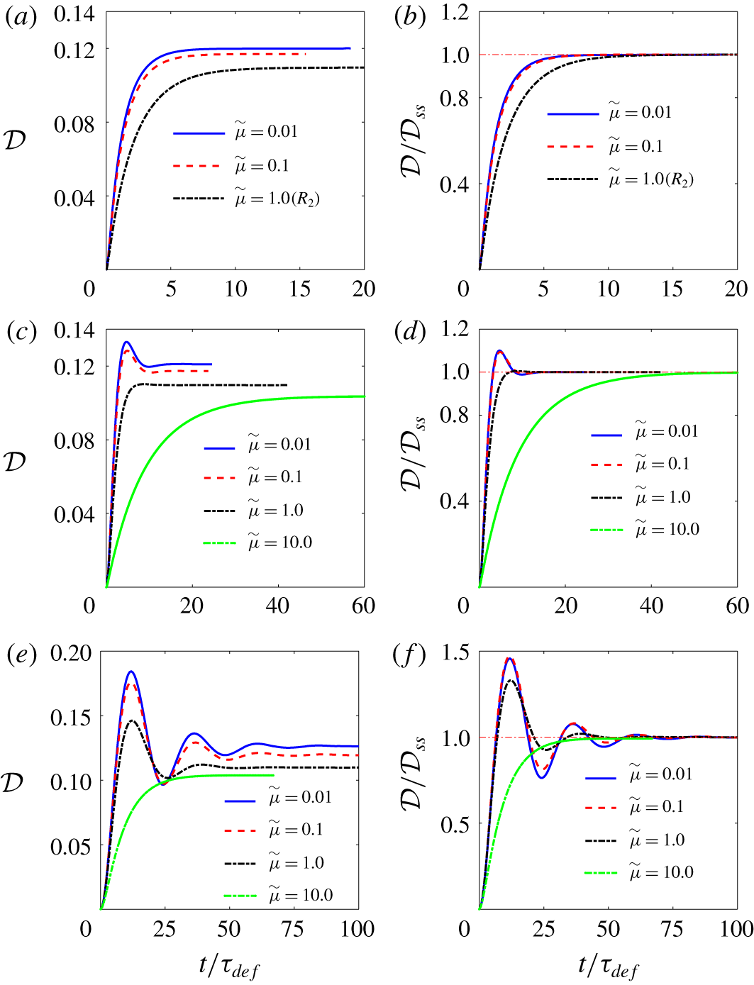
Evolution of deformation parameter with time at different capillary numbers for fluid system  $C$ for
 $Oh^{2}=2$, 0.2 and 0.02, corresponding to (a,b), (c,d) and (e,f), respectively. Here,
 $R_{3}$ in (a,b) denotes the reference simulation. For all the cases,
 $\widetilde{\unicode[STIX]{x1D70C}}=1$ and
 $\widetilde{\unicode[STIX]{x1D707}}=1$.

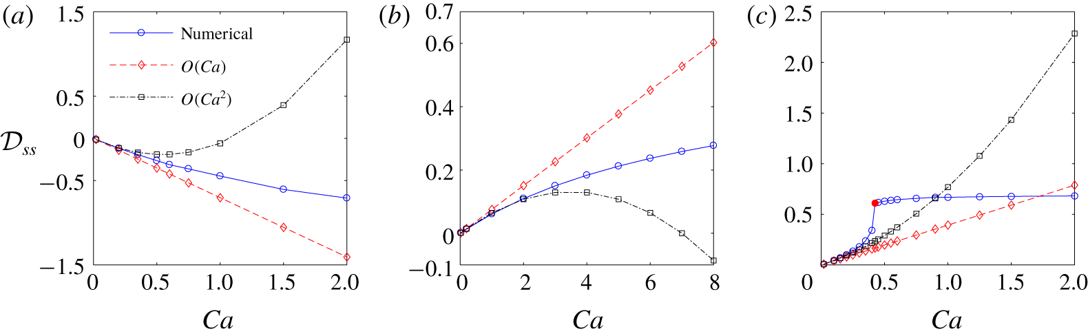
Figure 13 shows the steady-state deformation versus capillary number for the three fluid systems. Here, we present the results for  $Oh^{2}=0.02$ only, since the steady-state deformation is essentially independent of
 $Oh^{2}$. The results of the first- and second-order asymptotic solutions, equations (3.4) and (3.5), are also added to this figure. Here, the first-order asymptotic results agree with the results of the numerical simulation until
 ${\mathcal{D}}\approx 0.02$, 0.2 and 0.15, for fluid systems
 $A{-}C$, respectively. The agreement between the second-order asymptotic results and those of the numerical simulations holds up to 0.2, 2 and 0.25, for fluid systems
 $A{-}C$, respectively. The reason that the range of agreement of the asymptotic results with the numerical results is the largest for fluid system
 $B$ is because of the substantially smaller
 $k_{1}$ for this fluid system. This observation is in line with that of Feng & Scott (Reference Feng and Scott1996); see, their figure (5). For fluid systems
 $A$ and
 $B$, the deformation increases monotonically with the capillary number, as it should. On the other hand, for fluid system
 $C$, it gradually increases until
 $Ca\approx 0.4$, encounters a jump around
 $Ca=0.425$ and remains essentially constant due to the confinement effect. The direction of the curvature of the numerical curves (for fluid system
 $C$ the focus is up to
 $Ca\lessapprox 0.425$) are in line with the predictions of the second-order asymptotic solution. Here,
 $k_{2}$ is positive for fluid systems
 $A$ and
 $C$ and negative for fluid system
 $B$. Thus, the numerical curves are concave up for fluid systems
 $A$ and
 $C$, while the opposite holds for fluid system
 $B$. The sign of
 $k_{1}k_{2}$ provides some insight regarding the stability of the drop in an unbounded domain, where the deformation is not limited by the domain size. If
 $k_{1}k_{2}<0$, then the drop remains stable as the capillary number is increased; in this case, the drop elongates progressively in the direction of or perpendicular to the field, becoming prolate or oblate, respectively. On the other hand, if
 $k_{1}k_{2}>0$, the drop remains stable, or becomes unstable at a critical capillary number
 $Ca_{cr}$. If the drop remains stable, it will move along a hysteresis curve, where
 ${\mathcal{D}}-Ca$ curve transitions from
 $k_{1}k_{2}>0$ to
 $k_{1}k_{2}<0$ via an inflection point. For fluid systems
 $A$ and
 $B$,
 $k_{1}k_{2}<0$, therefore, the drop remains stable. This is hinted at by the signs (direction) of the curvatures of the
 ${\mathcal{D}}-Ca$ curve in these two cases. For fluid system
 $C$, the deformation progressively increases up to
 $Ca\approx 0.4$ and then encounters a jump somewhere between
 $Ca=0.4$ and 0.425.
Variation of steady-state deformation  ${\mathcal{D}}_{ss}$ with the capillary number
 $Ca$ for fluid systems
 $A{-}C$, corresponding to (a)–(c), respectively. For all the simulations,
 $Oh^{2}=0.02$.

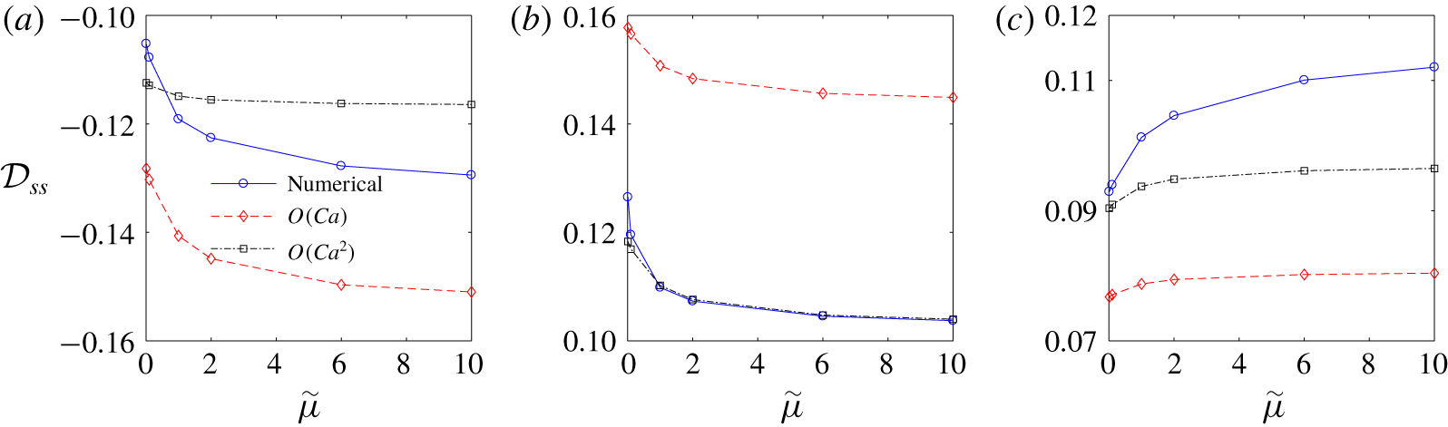
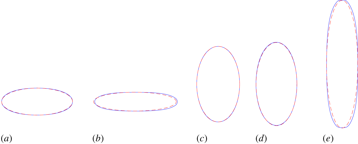
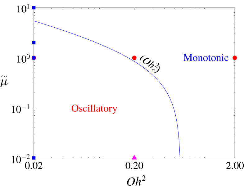
5.1.3 Effect of the viscosity ratio $\widetilde{\unicode[STIX]{x1D707}}$

The effect of the viscosity ratio on the transient electrohydrodynamics of leaky dielectric drops has not been studied in detail. However, several authors have explored this issue more thoroughly in the context of perfect dielectric fluid systems. Moriya, Adachi & Kotaka (Reference Moriya, Adachi and Kotaka1986), Nishiwaki, Adachi & Kotaka (Reference Nishiwaki, Adachi and Kotaka1988) and Haywood et al. (Reference Haywood, Renksizbulut and Raithby1991) focused on highly viscous liquid systems at low electric field strength for which deformation was small and the dynamic response was governed by only a time scale,  ${\mathcal{D}}={\mathcal{D}}_{ss}[1-\exp (-t/\unicode[STIX]{x1D70F})]$. The authors developed an expression for the time constant
 $\unicode[STIX]{x1D70F}$ in terms of the capillary time scale
 $\unicode[STIX]{x1D70F}_{def}=\unicode[STIX]{x1D707}_{o}a/\unicode[STIX]{x1D6FE}$ and the viscosity ratio
 $\widetilde{\unicode[STIX]{x1D707}}=\unicode[STIX]{x1D707}_{i}/\unicode[STIX]{x1D707}_{o}$, using heuristic arguments and analytical solutions. Supeene et al. (Reference Supeene, Koch and Bhattacharjee2004) studied the evolution of the drops using numerical simulations at low Ohnesorge numbers (
 $Oh\ll 1$), where the dynamic response was oscillatory. Considering a baseline simulation for which
 $\unicode[STIX]{x1D707}_{i}=\unicode[STIX]{x1D707}_{o}$, they observed that the dynamic response became more underdamped if they reduced the viscosity of the drop fluid
 $\unicode[STIX]{x1D707}_{i}$ or that of the ambient fluid
 $\unicode[STIX]{x1D707}_{o}$, while the latter rendered the dynamic response more oscillatory.
For steady state, the literature is limited to the studies by Feng & Scott (Reference Feng and Scott1996), Ha & Yang (Reference Ha and Yang2000) and Lac & Homsy (Reference Lac and Homsy2007). The focus of the first and the last studies was on the effect of  $\widetilde{\unicode[STIX]{x1D707}}$ on the critical capillary number
 $Ca_{cr}$ at which the drop disintegrates. Feng & Scott (Reference Feng and Scott1996) examined the effect of
 $\widetilde{\unicode[STIX]{x1D707}}$ on a prolate (
 $\widetilde{\unicode[STIX]{x1D70E}}=100$,
 $\widetilde{\unicode[STIX]{x1D716}}=2$, region II) and an oblate (
 $\widetilde{\unicode[STIX]{x1D70E}}=0.01$,
 $\widetilde{\unicode[STIX]{x1D716}}=0.5$, region I) drop at zero Reynolds number and concluded that in both cases increasing
 $\widetilde{\unicode[STIX]{x1D707}}$ shifted the critical field strength to a lower value. Lac & Homsy (Reference Lac and Homsy2007), on the other hand, examined prolate and oblate drops in creeping flow that were susceptible to instability (i.e. drops in regions I
 $^{-}$, II
 $^{+}$ and III
 $^{+}$, for which
 $k_{1}k_{2}>0$) and concluded that a ‘moderate’ increase in the viscosity ratio
 $\widetilde{\unicode[STIX]{x1D707}}$ shifted the critical field strength to a lower value in regions III
 $^{+}$ and I
 $^{-}$, while it had an opposite effect in region II
 $^{+}$. Ha & Yang (Reference Ha and Yang2000) developed experimentally the deformation-time curves for twenty one fluid systems with
 $0.001\leqslant \widetilde{\unicode[STIX]{x1D707}}\leqslant 0.874$. However, these authors did not elaborate on the effect of the viscosity ratio on the results. Similarly, no justification was provided by Feng & Scott (Reference Feng and Scott1996) and Lac & Homsy (Reference Lac and Homsy2007) to back up their observations. We note that, at small electric field strength (
 $Ca\ll 1$), the viscosity ratio has a weak influence on the degree of deformation of the leaky dielectric drops (Taylor Reference Taylor1964; Ajayi Reference Ajayi1978), while for the perfect dielectric fluid systems, the equilibrium shape is independent of the viscosity ratio, since fluid flow ceases to exist at steady state.
Evolution of the deformation parameter with time at different viscosity ratios  $\widetilde{\unicode[STIX]{x1D707}}$ for fluid system
 $A$. Here,
 $Oh^{2}=2$, 0.2 and 0.02 for (a,b), (c,d) and (e,f), respectively, and
 $Ca=0.2$ for all simulations. The deformation parameter has been scaled with the corresponding steady-state deformation
 ${\mathcal{D}}_{ss}$ for each case.

To explore the effect of the viscosity ratio on the behaviour of the drop, we performed several simulations at viscosity ratios  $\widetilde{\unicode[STIX]{x1D707}}$ above and below that of the reference simulations (
 $\widetilde{\unicode[STIX]{x1D707}}=1$). In these simulations, the viscosity ratio was changed by changing the viscosity of the drop fluid
 $\unicode[STIX]{x1D707}_{i}$. Figure 14 shows the deformation-time curves for fluid system
 $A$. For
 $Oh^{2}=2$, the result of the reference simulation
 $R_{1}$ (figure 5a) is identified in the figure. Since the ambient viscosity remains intact, the deformation time scale
 $\unicode[STIX]{x1D70F}_{def}=\unicode[STIX]{x1D707}_{o}a/\unicode[STIX]{x1D6FE}$ is the same for each set of simulations. Thus, the non-dimensionalization of the time does not affect the relative scales of the curves in a set. Furthermore, since the relaxation time to steady-state deformation (in monotonic response) and the oscillation period
 $\unicode[STIX]{x1D70F}_{\unicode[STIX]{x1D714}}$ (in oscillatory response) are inherent functions of viscosity ratio, the deformation curves in each set will not collapse to a single curve, even if their dynamic response corresponds to that of a linear mechanical system. Considering the left panels, it is seen that, for all simulations, the steady-state deformation
 $|{\mathcal{D}}|$ increases with an increase in
 $\widetilde{\unicode[STIX]{x1D707}}$. However, the rate of deformation with the viscosity ratio
 $\unicode[STIX]{x2202}|{\mathcal{D}}|/\unicode[STIX]{x2202}\widetilde{\unicode[STIX]{x1D707}}$ is small, which is hinted at by the asymptotic solution. For
 $Oh^{2}=2$, the dynamic response remains monotonic over three orders of magnitude of the viscosity ratio. Furthermore, the time constant at which the deformation settles to steady state increases with an increase in
 $\widetilde{\unicode[STIX]{x1D707}}$, which is in line with (5.2). For
 $Oh^{2}=0.2$, an order of magnitude decrease in the viscosity ratio from
 $\widetilde{\unicode[STIX]{x1D707}}=1$ to 0.1 leads to an oscillatory behaviour. However, another order of magnitude reduction does not lead to a major change in the dynamic response. For
 $Oh^{2}=0.02$, the dynamic response is already underdamped at
 $\widetilde{\unicode[STIX]{x1D707}}=1$. Here, an order of magnitude decrease in the viscosity ratio from
 $\widetilde{\unicode[STIX]{x1D707}}=1$ to 0.1 leads to a larger initial normalized peak. On the other hand, an order of magnitude increase in the viscosity ratio from
 $\widetilde{\unicode[STIX]{x1D707}}=1$ to 10 leads to transition of the dynamic response from an underdamped response to an overdamped one. It is seen that the differences between the dynamic responses for
 $\widetilde{\unicode[STIX]{x1D707}}=0.1$ and 0.01 in each set of curves are very small. This suggests that the dynamic response will be essentially independent of the viscosity ratio for
 $\widetilde{\unicode[STIX]{x1D707}}<0.01$. Hence,
 $\widetilde{\unicode[STIX]{x1D707}}=0.01$ may serve as the threshold for nearly inviscid fluid systems.
Figure 15 shows the deformation-time curves for fluid system  $B$. For
 $Oh^{2}=2$, the result of the reference simulation
 $R_{2}$, figure 5(b), is identified in the figure. Here, as opposed to fluid system
 $A$, the deformation decreases with an increase in
 $\widetilde{\unicode[STIX]{x1D707}}$. However, other features of the evolution are similar to those for fluid system
 $A$. Figure 16 shows the deformation-time curves for fluid system
 $C$. For
 $Oh^{2}=2$, the result of the reference simulation
 $R_{3}$ (figure 5c) is identified in the figure. Here, similar to fluid system
 $A$, the deformation increases with
 $\widetilde{\unicode[STIX]{x1D707}}$ for all fluid systems. Furthermore, the general features of the evolution are similar to those observed for fluid systems
 $A$ and
 $B$.
Evolution of the deformation parameter with time at different viscosity ratios  $\widetilde{\unicode[STIX]{x1D707}}$ for fluid system
 $B$. Here,
 $Oh^{2}=2$, 0.2 and 0.02 for (a,b), (c,d) and (e,f), respectively, and
 $Ca=2$ for all the simulations. The deformation parameter has been scaled with the corresponding steady-state deformation
 ${\mathcal{D}}_{ss}$ for each case.

Evolution of the deformation parameter with time at different viscosity ratios  $\widetilde{\unicode[STIX]{x1D707}}$ for fluid system
 $C$. Here,
 $Oh^{2}=2$, 0.2 and 0.02 for (a,b), (c,d) and (e,f), respectively, and
 $Ca=0.2$ for all the simulations. The deformation parameter has been scaled with the corresponding steady-state deformation
 ${\mathcal{D}}_{ss}$ for each case.

Figure 17 shows the steady-state deformation  ${\mathcal{D}}_{ss}$ versus the viscosity ratio
 $\widetilde{\unicode[STIX]{x1D707}}$ for fluid systems
 $A{-}C$. Here, we present the results for
 $Oh^{2}=0.02$ simulations only. This figure puts into perspective some of the features that we discussed earlier. An increase in
 $\widetilde{\unicode[STIX]{x1D707}}$ leads to an increase in
 $|{\mathcal{D}}|$ for fluid systems
 $A$ and
 $C$, but the opposite holds for fluid system
 $B$. These observations are in line with those of Lac & Homsy (Reference Lac and Homsy2007) who briefly touched on this issue. The rate of change of the deformation with the viscosity
 $\unicode[STIX]{x2202}|{\mathcal{D}}|/\unicode[STIX]{x2202}\widetilde{\unicode[STIX]{x1D707}}$ is higher for
 $0.01<\widetilde{\unicode[STIX]{x1D707}}<1$ compared to
 $\widetilde{\unicode[STIX]{x1D707}}>1$. We also superimpose the results of the asymptotic solution, equations (3.4) and (3.5), in this figure. Depending on the sign of
 $k_{1}k_{2}$, the second-order deformation
 $|{\mathcal{D}}_{\infty }^{\langle 2\rangle }|$ may be smaller or larger than the first-order one
 $|{\mathcal{D}}_{\infty }^{\langle 1\rangle }|$. Note that the capillary number
 $Ca$ is
 $0.2$ for fluid systems
 $A$ and
 $C$, while it is
 $2$ for fluid system
 $B$. Here, the correction for fluid system
 $B$ is marginal since
 $k_{2}<k_{1}\ll 1$. As expected, the second-order results show a closer agreement with the numerical results, compared to the first-order results, and the agreement between the two is better at
 $\widetilde{\unicode[STIX]{x1D707}}\lessapprox 0.1$. The agreement between the numerical and the analytical results is the best for fluid system
 $B$. This is primarily because of the reduction of
 $|{\mathcal{D}}|$ with
 $\widetilde{\unicode[STIX]{x1D707}}$ for this fluid system, which helps extend the range of applicability of the asymptotic results. In § 5.3 we provide the justification for the observed correlations between
 ${\mathcal{D}}_{ss}$ and
 $\widetilde{\unicode[STIX]{x1D707}}$ for the three fluid systems.
Variation of steady-state deformation  ${\mathcal{D}}_{ss}$ with the viscosity ratio
 $\widetilde{\unicode[STIX]{x1D707}}$ for fluid systems
 $A{-}C$, corresponding to (a)–(c), respectively. For all the simulations,
 $Oh^{2}=0.02$.

5.1.4 Ellipsoidal approximation
In the analytical studies of electrohydrodynamics of a liquid drop, the drop shape has been generally considered as an ellipsoid (Allan & Mason Reference Allan and Mason1962; Taylor Reference Taylor1964). This approximation seems to be reasonable for weak electric fields where  $|{\mathcal{D}}|\ll 1$, however, the ellipsoidal solution has been also used for strong electric fields, where the deformation is substantial. In particular, one can refer to the analytical solution of Bentenitis & Krause (Reference Bentenitis and Krause2005) who developed the so-called extended leaky dielectric method and solved the creeping flow equations using an ellipsoidal coordinates to study deformation of the drops in strong electric fields, and Zhang et al. (Reference Zhang, Zahn and Lin2013) who extended their approach to study transient deformation of drops, using numerical solution.
To explore whether the ellipsoidal approximation holds here, we found the cross-section of the drop in the  $y{-}z$ mid-plane for the simulations shown in figures 7, 9 and 11, and compared them with the contour of the counterpart ellipse,
 $$\begin{eqnarray}\frac{y^{2}}{(r_{max})^{2}}+\frac{z^{2}}{(z_{max})^{2}}=1,\end{eqnarray}$$
whose major (minor) and the minor (major) axes were equal to the maximum end-to-end length of the drop in the direction of the electric field  $z_{max}$ and its maximum breadth
 $r_{max}$ in the transverse direction. The relative error in the ellipsoidal approximation was measured by computing
 $E=1/N\sum _{i=1}^{N}|z_{n_{i}}-z_{a_{i}}|/z_{n_{i}}$, where
 $z_{n_{i}}$ and
 $z_{a_{i}}$ are the numerical and the approximated heights at the corresponding
 $y_{i}$,
 $N$ being the number of the points. Figure 18 shows the result of this comparison for representative simulations. Since the error increases with an increase in the capillary number, here we only present the results for the higher capillary numbers. Panels (a,b) pertain to fluid system
 $A$ at
 $Ca=1$ and 1.5. The agreement between the two curves seems excellent at
 $Ca=1$ but for
 $Ca=1.5$, the two differ around the left and the right ends. Here the relative error is approximately 0.37 % and 0.86 %, respectively. For
 $Ca=2$ (not shown here), the front deviated substantially from the elliptic shape. Panel (c) pertains to fluid system
 $B$ at
 $Ca=8$. Here, the two curves are nearly indistinguishable and the relative error is approximately 0.5 %. Panels (d,e) pertain to fluid system
 $C$ at
 $Ca=0.4$ and 0.45. For the former, which is before the onset of instability, the agreement between the two curves seems excellent and the relative error is approximately 2 %. For the latter, which is after the jump in the deformation and the squashing of the drop ends by the electrodes, the deviation between the two curves is substantial. Here, the error is 38 %. We speculate that, even for this more extreme elongated shape, the error would have been only a few per cent if it was characterized relative to an effective radius. Furthermore, the observed agreement should not be surprising, since higher modes in spherical harmonics will be suppressed by dissipation; see, for example, Yu et al. (Reference Yu, Lira, Riske, Dimova and Lin2015).
Comparison of the cross-section of the drop in the  $yz$ mid-plane with the corresponding ellipse. Panels (a) and (b) correspond, respectively, to panels (f) (
 $Ca=1$) and (g) (
 $Ca=1.5$) of figure 7. Panel (c) corresponds to panel (j) (
 $Ca=8$) of figure 9. Panels (d) and (e) correspond, respectively, to panels (g) (
 $Ca=0.4$) and (i) (
 $Ca=0.45$) of figure 11.

In the analysis of the effect of the capillary number on the dynamic response of the drops (figures 8, 10 and 12) the normalized curves followed the same trend with an increase in the capillary number for fluid system  $B$. However, this was not the case for fluid systems
 $A$ and
 $C$, where the curves followed two different trends at the low and the high capillary numbers. Considering figure 18, we believe the change in the trend for fluid system
 $A$ was primarily due to the deviation of the drop shape from the ellipsoidal shape at
 $Ca>1$. On the other hand, the change in the trend for fluid system
 $C$ was initially triggered by the transition of the deformation-time curve from a stable regime (
 $Ca\leqslant 0.4$) to an unstable one (
 $0.4<Ca\leqslant 0.425$). However, the deviation of the drop shape from the ellipsoidal shape also played a role later on, as soon as the drop began to touch the upper and the lower electrodes.
5.1.5 Deviation from linear response
In the analysis of the dynamic response of the drop at high  $Oh^{2}$ numbers (
 $Oh^{2}=2$) (figure 5) we observed that the numerical and analytical relaxation times had a nearly perfect agreement for the reference simulations
 $R_{1}$ and
 $R_{2}$, but the agreement was not so close for the reference simulation
 $R_{3}$. Recall that these simulations were based on fluid systems
 $A{-}C$, and their capillary numbers were
 $Ca=0.2$, 2 and 0.2, respectively.
Since the analytical solution is valid for the creeping flow regime ( $Re_{f}\ll 1$) and for small deformation (
 $Ca\ll 1$), one would normally expect the agreement between the numerical results and the analytical one to improve as the capillary number decreases. This is indeed the case for fluid system
 $C$ (figure 12b)) where the time constant of the
 $Ca=0.02$ curve is greater than the time constant of the reference simulation (
 $Ca=0.2$), which is smaller than the analytical time constant, as per figure 5(c). On the other hand, for fluid systems
 $A$ and
 $B$ (figures 8b and 10b) the agreement between the numerical results and the corresponding analytical ones decreases with a decrease in the capillary number, considering the fact that the deviation from the reference simulations
 $R_{1}$ (
 $Ca=0.2$) and
 $R_{2}$ (
 $Ca=8$) is tantamount to deviation from the analytical solutions, since the reference simulations had near perfect agreement with the corresponding analytical solution.
We believe that the trend seen here is primarily due to the convective effects that are present in the numerical simulations but absent in the analytical solution. While in our computations we do not explicitly account for the surface charge convection, this effect is possibly accounted for (to some degree) in the numerical simulation, where the coordinates of the marker points  $\boldsymbol{x}_{f}$ are moved by the kinematic equation
 $\text{d}\boldsymbol{x}_{f}/\text{d}t=\boldsymbol{u}_{f}$, where
 $\boldsymbol{u}_{f}$ is the grid velocity at their positions. Specifically, the movement of the marker points could account for the charge convection due to surface dilation (the second term in (2.6)). The presence of convective effects is further evidenced by the fact that in fluid systems
 $A$ and
 $B$, which show a similar trend, the direction of the external flow around the drop is the same (poles-to-equator), while in fluid system
 $C$, which shows the opposite trend, the flow runs in the opposite direction (equator-to-poles). Furthermore, in fluid system
 $C$, where the agreement between the numerical simulation and the analytical solution improves with the decrease in the capillary number (from 0.2 to 0.02), the results of computer simulations (not presented here) showed that an order of magnitude decrease in the capillary number from 0.02 to 0.002 did not improve the agreement; the results of
 $Ca=0.002$ simulation was essentially the same as that of the
 $Ca=0.02$ simulation. This hints at an effect that is present in the numerical simulation but absent in the analytical solution.
For fluid systems  $A$ and
 $B$, the marker points are moved by the fluid flow from the poles toward the equator, while for fluid system
 $C$, they are moved in the opposite direction. Because of the convective effects, the numerical time constant in general will not agree with the analytical solution, which ignores this effect. As pointed out by Feng (Reference Feng1999), the charge convection tends to decrease the deformation of the drops in regions I and II (fluid systems
 $A$ and
 $B$), while it tends to increase it in region III (fluid system
 $C$). Accordingly, for fluid systems
 $A$ and
 $B$, a combination of a capillary number that is not too small, along with the convective effects (which tend to reduce the deformation) leads to a time constant that is close to the analytical one. On the other hand, for fluid system
 $C$, where the convective effects tend to increase the deformation, a smaller capillary leads to a better agreement.
In summary, because of the sensitivity of the results to the instantaneous evolution of the drop, we believe the relaxation time  $\unicode[STIX]{x1D70F}_{rel}$ in the numerical solution
 ${\mathcal{D}}={\mathcal{D}}_{\infty }(1-\exp (-t/\unicode[STIX]{x1D70F}_{rel}))$ is a function of
 $\widetilde{\unicode[STIX]{x1D70E}}$,
 $\widetilde{\unicode[STIX]{x1D716}}$,
 $Ca$,
 $\unicode[STIX]{x1D70F}_{def}=\unicode[STIX]{x1D707}_{o}a/\unicode[STIX]{x1D6FE}$ and
 $\widetilde{\unicode[STIX]{x1D707}}$. On the other hand, the analytical time constant
 $\unicode[STIX]{x1D70F}_{a}\equiv \unicode[STIX]{x1D70F}$ is a function of
 $\unicode[STIX]{x1D70F}_{def}=\unicode[STIX]{x1D707}_{o}a/\unicode[STIX]{x1D6FE}$ and
 $\widetilde{\unicode[STIX]{x1D707}}$ only, as per (5.2). This leads to the observed mismatch. It is worth mentioning that the dependency of the time constant
 $\unicode[STIX]{x1D70F}$ on the capillary number
 $Ca$ and
 $\widetilde{\unicode[STIX]{x1D70E}}$ and
 $\widetilde{\unicode[STIX]{x1D716}}$ should be potentially unravelled from a second-order transient solution, and while Das & Saintillan (Reference Das and Saintillan2017b) provides such a solution, unfortunately, it is not possible to discern this dependency, since their solution is not in a closed form.
5.2 Characterizing the dynamic response by a second-order mechanical system model
From the investigations so far it is clear that the key parameters that determine the transition from a monotonic behaviour to an oscillatory one (or vice versa) for density-matched fluids are the Ohnesorge number squared  $Oh^{2}$ and the viscosity ratio
 $\widetilde{\unicode[STIX]{x1D707}}$, the former being more influential. In general, an oscillatory dynamic response is favoured by small
 $Oh^{2}$ and/or small
 $\widetilde{\unicode[STIX]{x1D707}}$. Conversely, a monotonic response is favoured by large
 $Oh^{2}$ and/or large
 $\widetilde{\unicode[STIX]{x1D707}}$. Theoretical characterization of the dynamic response of drops in these two limits provides valuable insight in exploring their behaviour. For small deformation
 $|{\mathcal{D}}|\ll 1$, this undertaking is possible using asymptotic solutions. For
 $Oh^{2}\gg 1$, the dynamic response can be characterized by (5.2), which is valid for creeping flows (
 $Re_{f}\ll 1$) and
 $\widetilde{\unicode[STIX]{x1D707}}=O(1)$. Here the dynamic response resembles that of a first-order linear overdamped mechanical system, where the response is controlled by only a time constant only. For
 $Oh^{2}\ll 1$, we resort to the Miller & Scriven (Reference Miller and Scriven1968) solution for small amplitude oscillations of a drop. These authors performed linear stability analysis along with normal mode approach to determine the stability of liquid drops (in the absence of an electric field) for arbitrary viscosity ratios subject to small surface perturbations. Subsequently, they simplified their generalized solution in the limit of
 $\unicode[STIX]{x1D707}_{i}$,
 $\unicode[STIX]{x1D707}_{o}\ll 1$ to characterize the drop oscillation in nearly inviscid fluid systems. Their oscillation frequency
 $\unicode[STIX]{x1D714}$ and the damping rate
 $\unicode[STIX]{x1D701}$ for an initially two-lobed (second-harmonic) oscillation read
 $$\begin{eqnarray}\displaystyle & \displaystyle \unicode[STIX]{x1D714}=\unicode[STIX]{x1D714}_{0}-\frac{25(\unicode[STIX]{x1D714}_{0}\unicode[STIX]{x1D707}_{i}\unicode[STIX]{x1D707}_{o}\unicode[STIX]{x1D70C}_{i}\unicode[STIX]{x1D70C}_{o})^{1/2}}{2^{1/2}\unicode[STIX]{x1D6EC}}, & \displaystyle\end{eqnarray}$$
 $$\begin{eqnarray}\displaystyle & \displaystyle \unicode[STIX]{x1D701}=\frac{25(\unicode[STIX]{x1D714}_{0}\unicode[STIX]{x1D707}_{i}\unicode[STIX]{x1D707}_{o}\unicode[STIX]{x1D70C}_{i}\unicode[STIX]{x1D70C}_{o})^{1/2}}{(2^{1/2})\unicode[STIX]{x1D6EC}}-\frac{625\unicode[STIX]{x1D707}_{i}\unicode[STIX]{x1D707}_{o}\unicode[STIX]{x1D70C}_{i}\unicode[STIX]{x1D70C}_{o}}{\unicode[STIX]{x1D6EC}^{2}}+\frac{5(6\unicode[STIX]{x1D707}_{i}^{2}\unicode[STIX]{x1D70C}_{i}+16\unicode[STIX]{x1D707}_{o}^{2}\unicode[STIX]{x1D70C}_{o}+\unicode[STIX]{x1D707}_{i}\unicode[STIX]{x1D707}_{o}(4\unicode[STIX]{x1D70C}_{i}-\unicode[STIX]{x1D70C}_{o}))}{2a^{2}\unicode[STIX]{x1D6E4}((\unicode[STIX]{x1D707}_{i}\unicode[STIX]{x1D70C}_{i})^{1/2}+(\unicode[STIX]{x1D707}_{o}\unicode[STIX]{x1D70C}_{o})^{1/2})}, & \displaystyle \nonumber\\ \displaystyle & & \displaystyle\end{eqnarray}$$
 $$\begin{eqnarray}\displaystyle & \displaystyle \unicode[STIX]{x1D714}_{0}=\sqrt{\frac{24}{3\widetilde{\unicode[STIX]{x1D70C}}+2}\left(\frac{\unicode[STIX]{x1D6FE}}{\unicode[STIX]{x1D70C}_{o}a^{3}}\right)}, & \displaystyle\end{eqnarray}$$
 $$\begin{eqnarray}\displaystyle & \displaystyle \unicode[STIX]{x1D6EC}=2a\unicode[STIX]{x1D6E4}((\unicode[STIX]{x1D707}_{i}\unicode[STIX]{x1D70C}_{i})^{1/2}+(\unicode[STIX]{x1D707}_{o}\unicode[STIX]{x1D70C}_{o})^{1/2}), & \displaystyle\end{eqnarray}$$
 $$\begin{eqnarray}\displaystyle & \displaystyle \unicode[STIX]{x1D6E4}=2\unicode[STIX]{x1D70C}_{o}+3\unicode[STIX]{x1D70C}_{i}, & \displaystyle\end{eqnarray}$$
 $\unicode[STIX]{x1D714}_{0}$ is the frequency of oscillation for inviscid fluids (Lamb Reference Lamb1932). Note that the inclusion of the second term in (5.4b) was suggested by Marston (Reference Marston1980), Prosperetti (Reference Prosperetti1980) and Basaran, Scott & Byers (Reference Basaran, Scott and Byers1989), who re-derived the solution of Miller & Scriven independently. Furthermore, Prosperetti pointed out that, in order for (5.4) to be valid, not only should the viscosities be small (
 $\unicode[STIX]{x1D707}_{i},\unicode[STIX]{x1D707}_{o}\ll 1$), but also their orders should be the same,
 $O(\unicode[STIX]{x1D707}_{i})=O(\unicode[STIX]{x1D707}_{o})$. He also provided an estimate of the error by comparison of the results of (5.4) with that of the exact solution of the dispersion relation for a few cases and concluded that the error will be negligibly small for
 $Oh_{i}^{2}$,
 $Oh_{o}^{2}<0.01$. However, he estimated that an order of magnitude increase in
 $Oh_{i}^{2}$ and
 $Oh_{o}^{2}$, would lead to a ten per cent error with respect to the exact solution.
Here, we use (5.4) to construct an equation for  ${\mathcal{D}}(t)$ by considering
 ${\mathcal{D}}(t)={\mathcal{D}}_{\infty }[1+\exp (-\unicode[STIX]{x1D701}t)(c_{1}\cos \unicode[STIX]{x1D714}t+c_{2}\sin \unicode[STIX]{x1D714}t)]$, where
 $\unicode[STIX]{x1D701}$ and
 $\unicode[STIX]{x1D714}$ are given in (5.4) and
 $c_{1}$ and
 $c_{2}$ are found from
 ${\mathcal{D}}(0)=0$ and
 $\text{d}{\mathcal{D}}(0)/\text{d}t=0$. This leads to
 $$\begin{eqnarray}{\mathcal{D}}={\mathcal{D}}_{\infty }\left[1-\exp (-\unicode[STIX]{x1D701}t)\left(\cos \unicode[STIX]{x1D714}t+\left(\frac{\unicode[STIX]{x1D701}}{\unicode[STIX]{x1D714}}\right)\sin \unicode[STIX]{x1D714}t\right)\right],\end{eqnarray}$$
which we will use as the equation that represents the dynamic response in the limit of small  $Oh^{2}$ and
 $\widetilde{\unicode[STIX]{x1D707}}$. Equation (5.5) characterizes the behaviour of a second-order underdamped linear mechanical system. In passing, we note that the solution of Miller & Scriven (Reference Miller and Scriven1968) for high viscosities (their equation (38)) converges to (5.2) by setting
 $\ell =2$,
 $\ell$ being the mode number of the oscillation.
A question that naturally arises is whether it is possible to find a priori a criterion that identifies transition from a monotonic response to an oscillatory one (or vice versa). To construct a solution that is reasonably accurate in the intermediate range of  $Oh^{2}$ and converges to (5.2) and (5.5) for
 $Oh^{2}\gg 1$ and
 $Oh^{2}\ll 1$, respectively, we consider a differential equation of the from
 $$\begin{eqnarray}c_{1}\frac{\text{d}^{2}{\mathcal{D}}}{\text{d}t^{2}}+c_{2}\left(\unicode[STIX]{x1D70F}\frac{\text{d}{\mathcal{D}}}{\text{d}t}+{\mathcal{D}}\right)=c_{2}{\mathcal{D}}_{\infty },\end{eqnarray}$$
where  $c_{1}$ and
 $c_{2}$ are positive constants and
 $\unicode[STIX]{x1D70F}$ is the time constant defined in (5.2b). This equation is formally the same as that for a general second-order mechanical system and its structure is inspired by the fact that for
 $c_{1}\rightarrow 0$, it converges to the differential equation corresponding to (5.2). Here,
 $c_{1}$ and
 $c_{2}$ are found by matching them in the limit of
 ${\mathcal{D}}_{\infty }\rightarrow 0$ and
 $\unicode[STIX]{x1D70F}\rightarrow 0$ with the corresponding coefficients in the classical equation concerning the free oscillation of an inviscid drop (Lamb Reference Lamb1932)
 $$\begin{eqnarray}\frac{1}{\unicode[STIX]{x1D714}_{0}}\frac{\text{d}^{2}{\mathcal{D}}}{\text{d}t^{2}}+{\mathcal{D}}=0.\end{eqnarray}$$
This results in  $c_{1}=1/\unicode[STIX]{x1D714}_{0}^{2}$ and
 $c_{2}=1$. Substitution for these coefficients in (5.6) yields
 $$\begin{eqnarray}\frac{1}{\unicode[STIX]{x1D714}_{0}^{2}}\frac{\text{d}^{2}{\mathcal{D}}}{\text{d}t^{2}}+\unicode[STIX]{x1D70F}\frac{\text{d}{\mathcal{D}}}{\text{d}t}+{\mathcal{D}}={\mathcal{D}}_{\infty },\end{eqnarray}$$
as the governing equation for the evolution of the drop deformation in the limit of small deformation for arbitrary  $Oh^{2}$. The solution of (5.8), subject to initial conditions
 ${\mathcal{D}}(0)=0$ and
 $\unicode[STIX]{x2202}{\mathcal{D}}/\unicode[STIX]{x2202}t(0)=0$, yields
 $$\begin{eqnarray}\displaystyle & \displaystyle {\mathcal{D}}(t)={\mathcal{D}}_{\infty }\left[1-\exp \left(-{\displaystyle \frac{\unicode[STIX]{x1D70F}\unicode[STIX]{x1D714}_{0}^{2}}{2}}t\right)\left(\cos (\unicode[STIX]{x1D714}_{d}t)+{\displaystyle \frac{\unicode[STIX]{x1D70F}\unicode[STIX]{x1D714}_{0}^{2}}{2\unicode[STIX]{x1D714}_{d}}}\sin (\unicode[STIX]{x1D714}_{d}t)\right)\right];\quad \unicode[STIX]{x1D70F}\unicode[STIX]{x1D714}_{0}/2<1,\qquad & \displaystyle\end{eqnarray}$$
 $$\begin{eqnarray}\displaystyle & \displaystyle \unicode[STIX]{x1D714}_{d}=\unicode[STIX]{x1D714}_{0}\sqrt{1-\left(\frac{\unicode[STIX]{x1D70F}\unicode[STIX]{x1D714}_{0}}{2}\right)^{2}}, & \displaystyle\end{eqnarray}$$
 $$\begin{eqnarray}\displaystyle & \displaystyle {\mathcal{D}}(t)={\mathcal{D}}_{\infty }\left[1+{\displaystyle \frac{\unicode[STIX]{x1D706}_{2}}{\unicode[STIX]{x1D706}_{1}-\unicode[STIX]{x1D706}_{2}}}\exp (-\unicode[STIX]{x1D706}_{1}t)-{\displaystyle \frac{\unicode[STIX]{x1D706}_{1}}{\unicode[STIX]{x1D706}_{1}-\unicode[STIX]{x1D706}_{2}}}\exp (-\unicode[STIX]{x1D706}_{2}t)\right];\quad \unicode[STIX]{x1D70F}\unicode[STIX]{x1D714}_{0}/2>1,\qquad & \displaystyle\end{eqnarray}$$
 $$\begin{eqnarray}\displaystyle & \displaystyle \unicode[STIX]{x1D706}_{1,2}=\frac{\unicode[STIX]{x1D70F}\unicode[STIX]{x1D714}_{0}^{2}}{2}\mp \unicode[STIX]{x1D714}_{0}\sqrt{\left(\frac{\unicode[STIX]{x1D70F}\unicode[STIX]{x1D714}_{0}}{2}\right)^{2}-1};\quad \unicode[STIX]{x1D70F}\unicode[STIX]{x1D714}_{0}/2>1, & \displaystyle\end{eqnarray}$$
 $\unicode[STIX]{x1D714}_{d}$ is the underdamped angular frequency of the system, and
 $\unicode[STIX]{x1D706}_{1}$ and
 $\unicode[STIX]{x1D706}_{2}$ are the characteristic times for monotonic decay (i.e. overdamped deformation). As is evident, the transition from a monotonic dynamic response to an oscillatory one (and vice versa) is determined by the magnitude of
 $\unicode[STIX]{x1D70F}\unicode[STIX]{x1D714}_{0}/2$ relative to one. Thus, setting
 $\unicode[STIX]{x1D70F}\unicode[STIX]{x1D714}_{0}/2=1$ leads to
 $$\begin{eqnarray}Oh_{c}^{2}=\frac{3\widetilde{\unicode[STIX]{x1D70C}}+2}{6}\left[\frac{40(\widetilde{\unicode[STIX]{x1D707}}+1)}{(19\widetilde{\unicode[STIX]{x1D707}}+16)(2\widetilde{\unicode[STIX]{x1D707}}+3)}\right]^{2}\end{eqnarray}$$
as the characteristic Ohnesorge number (squared) for which the solution switches from an overdamped response ( $Oh^{2}>Oh_{c}^{2}$) to an underdamped one (
 $Oh^{2}<Oh_{c}^{2}$). Considering the fact that
 $Oh_{c}^{2}$ is a decreasing function of
 $\widetilde{\unicode[STIX]{x1D707}}$ and an increasing function of
 $\widetilde{\unicode[STIX]{x1D70C}}$, and that a higher
 $Oh_{c}^{2}$ is tantamount to a liquid drop that more readily becomes oscillatory, all things being the same, the oscillatory behaviour is favoured toward the drops less viscous and more dense than the surrounding fluid. This observation reaffirms the result of the non-dimensionalization of the momentum equation in § 5.1.1. Figure 19 presents these observations in terms of a phase diagram for density-matched fluids.
A phase diagram depicting the regions of the monotonic and oscillatory responses in the physical space. The characteristic Ohnesorge number squared ( $Oh_{c}^{2}$) is found from (5.11). The symbols represent the placement on the map of the numerical results in § 5.2. Here, the circle, the square and the triangle represent the results of figures 20–22, respectively.

In the investigations that we performed to explore the performance of (5.9), the agreement between (5.9) and the numerical results would improve substantially if in (5.9) the inviscid frequency  $\unicode[STIX]{x1D714}_{0}$ and the underdamped frequency
 $\unicode[STIX]{x1D714}_{d}$ were replaced with the nearly inviscid frequency
 $\unicode[STIX]{x1D714}$ and
 $\widehat{\unicode[STIX]{x1D714}}_{d}\equiv \unicode[STIX]{x1D714}\sqrt{1-(\unicode[STIX]{x1D70F}\unicode[STIX]{x1D714}/2)^{2}}$, while keeping the damping rate intact. This yields
 $$\begin{eqnarray}\displaystyle & \displaystyle {\mathcal{D}}(t)={\mathcal{D}}_{\infty }\left[1-\exp \left(-{\displaystyle \frac{\unicode[STIX]{x1D70F}\unicode[STIX]{x1D714}_{0}^{2}}{2}}t\right)\left(\cos (\widehat{\unicode[STIX]{x1D714}}_{d}t)+{\displaystyle \frac{\unicode[STIX]{x1D70F}\unicode[STIX]{x1D714}^{2}}{2\widehat{\unicode[STIX]{x1D714}}_{d}}}\sin (\widehat{\unicode[STIX]{x1D714}}_{d}t)\right)\right];\quad \unicode[STIX]{x1D70F}\unicode[STIX]{x1D714}/2<1,\qquad & \displaystyle\end{eqnarray}$$
 $$\begin{eqnarray}\displaystyle & \displaystyle \widehat{\unicode[STIX]{x1D714}}_{d}=\unicode[STIX]{x1D714}\sqrt{1-\left(\frac{\unicode[STIX]{x1D70F}\unicode[STIX]{x1D714}}{2}\right)^{2}}, & \displaystyle\end{eqnarray}$$
 $Oh_{i}^{2}$,
 $Oh_{o}^{2}\ll 1$,
 $\unicode[STIX]{x1D707}_{i}$,
 $\unicode[STIX]{x1D707}_{o}\ll 1$ and
 $O(\unicode[STIX]{x1D707}_{i})=O(\unicode[STIX]{x1D707}_{o})$. We note that, since
 $\widehat{\unicode[STIX]{x1D714}}_{d}/\unicode[STIX]{x1D714}\leqslant 1$, the frequency of oscillation predicted by (5.12) is in general less than that of (5.5). On the other hand, the relative magnitude of the damping rates of (5.5) and (5.12),
 $\unicode[STIX]{x1D70F}\unicode[STIX]{x1D714}_{0}^{2}/2$ and
 $\unicode[STIX]{x1D701}$, depends on the viscosity ratio. From this point onward, we refer to (5.2) as E & S, equation (5.5) as M & S and (5.10) and (5.12) as the generalized mechanical system solutions (GMS-O and GMS-U), where O and U stand for overdamped and underdamped.
Comparison of the dynamic response of a drop in fluid system  $B$ with the pertinent asymptotic solutions, E & S (5.2) and M & S (5.5) and the generalized solution, GMS-O (5.10) and GMS-U (5.12). The capillary number is
 $Ca=0.02$ and
 $Oh^{2}$ is 2, 0.2 and 0.02, corresponding to (a)–(c), respectively.

To scrutinize the performance of the generalized solution, equations (5.10) and (5.12), in predicting the monotonic and oscillatory responses, respectively, we compared it with the results of our numerical simulations as well as the asymptotic solutions, equations (5.2) and (5.5). This comparison covered three orders of magnitude of the Ohnesorge number squared ( $Oh^{2}=0.02{-}2$) and the capillary number (
 $Ca=0.02{-}2$) and four orders of magnitude of the viscosity ratio (
 $\widetilde{\unicode[STIX]{x1D707}}=0.01{-}10$). As the focus of these tests was on the temporal evolution of the deformation parameter (i.e. monotonic versus oscillatory), we used the normalized deformations;
 ${\mathcal{D}}/{\mathcal{D}}_{ss}$ for the numerical simulation and
 ${\mathcal{D}}/{\mathcal{D}}_{\infty }$ for the generalized and the asymptotic solutions. These investigations showed that the generalized solution performed the best at both ends of the spectra (
 $Oh^{2}\ll 1$ and
 $Oh^{2}\gg 1$) for viscosity-matched fluid systems
 $\widetilde{\unicode[STIX]{x1D707}}=1$. It also performed reasonably well for
 $Oh^{2}\ll 1$ and
 $0.1<\widetilde{\unicode[STIX]{x1D707}}<1$, and at intermediate
 $Oh^{2}$ (
 $Oh^{2}\lessapprox 1$) at
 $\widetilde{\unicode[STIX]{x1D707}}=1$. However, it did not perform very well for
 $Oh^{2}\ll 1$ and
 $\widetilde{\unicode[STIX]{x1D707}}\ll 1$. We note that the less than optimal performance of the generalized solution (5.12) in this range is because this equation is being used outside its realm of validity.
Here, we present the results of some of these investigations. Figure 20 shows representative results for fluid system  $B$ over three orders of magnitude of
 $Oh^{2}$. Here,
 $Ca=0.02$ and
 $\widetilde{\unicode[STIX]{x1D707}}=1$. In this figure and the one that will follow,
 ${\mathcal{D}}_{c}$ stands for characteristic deformation, where
 ${\mathcal{D}}_{c}\equiv {\mathcal{D}}_{ss}$ for the numerical simulation and
 ${\mathcal{D}}_{c}\equiv {\mathcal{D}}_{\infty }$ for the generalized and the asymptotic solutions. For
 $Oh^{2}=2$ and
 $Oh^{2}=0.02$, the generalized solutions are in close agreement with the numerical results and also converge to the asymptotic solutions. For
 $Oh^{2}=0.2$, the dynamic response is overdamped and resembles a second-order mechanical system, because of the existence of an inflection point during the transient period. Here, the generalized solution picks up the correct (monotonic) branch, however, since the analytical time constants (
 $1/\unicode[STIX]{x1D706}_{1}$ and
 $1/\unicode[STIX]{x1D706}_{2}$) do not quite match the intrinsic time constants of the numerical solution, there are some differences between the two. Figure 21 shows representative results for fluid system
 $B$ over four orders of magnitude of the viscosity ratio
 $\widetilde{\unicode[STIX]{x1D707}}=0.01{-}10$. Here,
 $Oh^{2}=0.02$ and
 $Ca=2$. As is evident, the discrepancy between the generalized and asymptotic solutions and the numerical result is the largest at
 $\widetilde{\unicode[STIX]{x1D707}}=0.01$. However, compared to the asymptotic solution, the generalized solution follows the numerical curve more closely. The agreement between the generalized and asymptotic solutions and the numerical result improves substantially for
 $\widetilde{\unicode[STIX]{x1D707}}=1$ and starts to decline for
 $\widetilde{\unicode[STIX]{x1D707}}>1$. For
 $\widetilde{\unicode[STIX]{x1D707}}=10$ the dynamic response becomes monotonic and the generalized solution (5.10) and the asymptotic one (5.2) are in close agreement. However, both solutions overestimate the relaxation time. Figure 22 shows representative results for fluid systems
 $A{-}C$ at an intermediate
 $Oh^{2}$ (
 $Oh^{2}=0.2$) and
 $\widetilde{\unicode[STIX]{x1D707}}=0.01$. Here,
 $Ca=0.2$, 2 and 0.2, respectively. The asymptotic solution (5.5) grossly overestimates the damping rates for all the fluid systems, leading to dynamic responses that are essentially monotonic. On the other hand, the generalized solution (5.12) mimics the numerical simulations more closely. Both solutions, however, have a phase lead with respect to the numerical curve. Figure 19 shows the placement of the numerical simulations on the phase diagram, where it is seen that the prediction of (5.11) in demarking the monotonic and oscillatory response is correct for all the numerical simulations.
Comparison of the dynamic response of a drop in fluid system  $B$ at
 $Oh^{2}=0.02$ and
 $Ca=2$ with the creeping flow solution, E & S (5.2), the solution for nearly inviscid drops, M & S (5.5) and the generalized solution, GMS-O (5.10) and GMS-U (5.12). The viscosity ratios are
 $\widetilde{\unicode[STIX]{x1D707}}=0.01$, 1 and 10, corresponding to (a)–(c), respectively.

Comparison of the dynamic response of a drop in fluid systems  $A{-}C$ (a–c) at
 $Oh^{2}=0.2$ and
 $\widetilde{\unicode[STIX]{x1D707}}=0.01$ with the solution for nearly inviscid drops, M & S (5.5) and the generalized solution, GMS-U (5.12). Here,
 $Ca=0.2$, 2 and 0.2, for fluid systems
 $A{-}C$, respectively.

5.3 The normal stress map
In the studies on the electrohydrodynamics of a liquid drop, there are two main misconceptions about the relative strength of the hydrodynamic and electric forces and their interplay. Specifically, it is presumed that the drop deforms to an oblate shape because of stronger hydrodynamic forces relative to the electric pressure, and that the electric pressure always tends to deform a drop to a prolate: ‘…oblate drop deformation usually indicates relatively high flow intensity, because the oblate drop shape is necessarily maintained by the hydrodynamic stresses arising from the flow field against the normal electric stress that always tend to deform the drop into prolate shape …’, in Feng & Scott (Reference Feng and Scott1996, p. 307); ‘…it is worth pointing out that the electrical normal stress mismatch would always deform the drop into a prolate spheroid …’, in Ha & Yang (Reference Ha and Yang1995, p. 366); ‘…by its nature, the oblate regime is characterized by important electrohydrodynamic effects, since the drop is always prolate when these effects vanish …’, in Lac & Homsy (Reference Lac and Homsy2007, p. 262). In what follows we try to mitigate these misconceptions by resorting to the small-deformation theory (Taylor Reference Taylor1966). This undertaking also provides the reason behind the trend seen in figure 17, concerning the variation of the steady-state deformation with the viscosity ratio, as the two topics are indeed related.
We note that the sense and degree of the deformation of the drop is set by the normal electric stress (also called electric pressure)  $\unicode[STIX]{x27E6}\unicode[STIX]{x1D70F}_{nn}^{e}\unicode[STIX]{x27E7}$ and the hydrodynamic stress
 $\unicode[STIX]{x27E6}\unicode[STIX]{x1D70E}_{nn}^{h}\unicode[STIX]{x27E7}\equiv \unicode[STIX]{x27E6}\unicode[STIX]{x1D70F}_{nn}^{h}\unicode[STIX]{x27E7}-\unicode[STIX]{x27E6}\,p\unicode[STIX]{x27E7}$. To explore the interplay of these forces in the drop deformation, we decompose the deformation characteristic function
 $\unicode[STIX]{x1D6F7}$ (3.4c) into two parts:
 $$\begin{eqnarray}\displaystyle & \displaystyle \unicode[STIX]{x1D6F7}=\unicode[STIX]{x1D6F7}^{e}+\unicode[STIX]{x1D6F7}^{h}, & \displaystyle\end{eqnarray}$$
 $$\begin{eqnarray}\displaystyle & \displaystyle \unicode[STIX]{x1D6F7}^{e}=\widetilde{\unicode[STIX]{x1D70E}}^{2}+1-2\widetilde{\unicode[STIX]{x1D716}},\quad \unicode[STIX]{x1D6F7}^{h}=\frac{3}{5}\frac{3\widetilde{\unicode[STIX]{x1D707}}+2}{\widetilde{\unicode[STIX]{x1D707}}+1}(\widetilde{\unicode[STIX]{x1D70E}}-\widetilde{\unicode[STIX]{x1D716}}), & \displaystyle\end{eqnarray}$$
 $\unicode[STIX]{x1D6F7}^{e}$ and
 $\unicode[STIX]{x1D6F7}^{h}$ represent the contributions of the anisotropic components of the electric pressure and normal hydrodynamic stress in the deformation, respectively. The collective effect of
 $\unicode[STIX]{x1D6F7}^{e}$ and
 $\unicode[STIX]{x1D6F7}^{h}$ on the deformation can be best understood by considering the relative importance of these stresses in the different regions of the deformation–circulation map. To do so, we construct a map in a
 $\widetilde{\unicode[STIX]{x1D716}}-\widetilde{\unicode[STIX]{x1D70E}}$ coordinate where we draw the zero-deformation curve (
 $\unicode[STIX]{x1D6F7}=0$) along with the
 $\unicode[STIX]{x1D719}^{e}=0$ curve, the
 $\unicode[STIX]{x1D6F7}^{h}=0$ line and the
 $|\unicode[STIX]{x1D6F7}^{e}|=|\unicode[STIX]{x1D6F7}^{h}|$ curve (figure 23). Note that the
 $\unicode[STIX]{x1D6F7}^{h}=0$ line is indeed the zero-circulation (
 $\widetilde{\unicode[STIX]{x1D70E}}=\widetilde{\unicode[STIX]{x1D716}}$) line. Thus, along the
 $\unicode[STIX]{x1D719}^{e}=0$ curve and the
 $\unicode[STIX]{x1D6F7}^{h}=0$ line, the contribution of the electric pressure and the hydrodynamic force is zero, respectively. The
 $\unicode[STIX]{x1D6F7}^{e}=0$ curve runs essentially parallel to the
 $\unicode[STIX]{x1D6F7}=0$ curve and almost coincides with that curve in the
 $\widetilde{\unicode[STIX]{x1D716}}>1$ region of the map. The
 $\unicode[STIX]{x1D6F7}^{e}=0$ curve and the
 $\unicode[STIX]{x1D6F7}^{h}=0$ line are used to identify the change in direction of the electric pressure and the hydrodynamic normal stress, where positive or negative
 $\unicode[STIX]{x1D6F7}^{e}$ (
 $\unicode[STIX]{x1D6F7}^{h}$) is interpreted as the normal electric (hydrodynamic) stress that tends to deform the drop to a prolate or an oblate, respectively. When the signs of
 $\unicode[STIX]{x1D6F7}^{e}$ and
 $\unicode[STIX]{x1D6F7}^{h}$ are the same, the sense of the drop deformation can be readily determined. However, when the sign of
 $\unicode[STIX]{x1D6F7}^{e}$ and
 $\unicode[STIX]{x1D6F7}^{h}$ are opposite, to determine the sense of drop deformation, the relative magnitude of
 $\unicode[STIX]{x1D6F7}^{e}$ and
 $\unicode[STIX]{x1D6F7}^{h}$ needs to be known. This information can be extracted from the
 $|\unicode[STIX]{x1D6F7}^{e}|=|\unicode[STIX]{x1D6F7}^{h}|$ curve, which is the locus of the points where the contributions of the normal electric and hydrodynamic stresses are equal. Two possibilities exist: if
 $\unicode[STIX]{x1D6F7}^{e}\unicode[STIX]{x1D6F7}^{h}<0$, then the
 $|\unicode[STIX]{x1D6F7}^{e}|=|\unicode[STIX]{x1D6F7}^{h}|$ curve is simply the
 $\unicode[STIX]{x1D6F7}=0$ curve, since
 $|\unicode[STIX]{x1D6F7}^{e}|=|\unicode[STIX]{x1D6F7}^{h}|$ leads to
 $\unicode[STIX]{x1D6F7}^{e}=-\unicode[STIX]{x1D6F7}^{h}$, or
 $\unicode[STIX]{x1D6F7}^{e}+\unicode[STIX]{x1D6F7}^{h}\equiv \unicode[STIX]{x1D6F7}=0$. On the other hand, if
 $\unicode[STIX]{x1D6F7}^{e}\unicode[STIX]{x1D6F7}^{h}>0$, then the equation of the curve will be
 $\unicode[STIX]{x1D6F7}^{e}=\unicode[STIX]{x1D6F7}^{h}$, which is shown by the dotted line in the figure.
The electric pressure-normal hydrodynamic stress map, which is used to determine the signs and the relative strengths of the electric pressure  $\unicode[STIX]{x27E6}\unicode[STIX]{x1D70F}_{nn}^{e}\unicode[STIX]{x27E7}$ and the normal hydrodynamic stress
 $\unicode[STIX]{x27E6}\unicode[STIX]{x1D70F}_{nn}^{h}\unicode[STIX]{x27E7}$;
 $\unicode[STIX]{x27E6}\unicode[STIX]{x1D70F}_{nn}^{h}\unicode[STIX]{x27E7}$ is dominant only in the shaded subregions of region I, i.e.
 $\text{I}_{NN}^{h}$ and
 $\text{I}_{PN}^{h}$. The senses of the normal hydrodynamic stress and the electric pressure are the same in regions
 $\text{III}\equiv \text{III}_{PP}^{e}$,
 $\text{I}_{NN}^{h}$ and
 $\text{I}_{NN}^{e}$, and in the opposite directions in regions
 $\text{I}_{PN}^{h}$ and
 $\text{II}\equiv \text{II}_{PN}^{e}$.

The information provided by the  $\unicode[STIX]{x1D6F7}=0$,
 $\unicode[STIX]{x1D6F7}^{e}=0$,
 $\unicode[STIX]{x1D6F7}^{h}=0$ and
 $|\unicode[STIX]{x1D6F7}^{e}|=|\unicode[STIX]{x1D6F7}^{h}|$ curves can be used to infer the signs of
 $\unicode[STIX]{x1D6F7}^{e}$ and
 $\unicode[STIX]{x1D6F7}^{h}$ and their relative strengths in the different regions of the map. The
 $\unicode[STIX]{x1D6F7}=0$ curve and the
 $\unicode[STIX]{x1D6F7}^{h}=0$ line divide the map into three regions I–III, which are exactly the same as the corresponding regions in the deformation–circulation map, and are named the same way. Furthermore, the curves
 $\unicode[STIX]{x1D6F7}^{e}=0$ and
 $|\unicode[STIX]{x1D6F7}^{e}|=|\unicode[STIX]{x1D6F7}^{h}|$ (when
 $\unicode[STIX]{x1D6F7}^{e}\unicode[STIX]{x1D6F7}^{h}>0$) divide region I into subregions I
 $_{NN}^{e}$, I
 $_{NN}^{h}$ and I
 $_{PN}^{h}$. In naming these subregions we have used R
 $_{ij}^{k}$, where R stands for the region, superscript
 $k$ refers to the dominance of the electric
 $(e)$ or the hydrodynamic
 $(h)$ stresses, respectively, and subscripts
 $i$ and
 $j$ refer to the signs of
 $\unicode[STIX]{x1D6F7}^{e}$ and
 $\unicode[STIX]{x1D6F7}^{h}$, respectively. Note that a positive
 $(P)$ or a negative
 $(N)$ normal stress tends to deform the drop to a prolate or an oblate, respectively. Accordingly, in subregions I
 $_{NN}^{e}$ and I
 $_{NN}^{h}$ both electric pressure and normal hydrodynamic stresses tend to deform the drop to an oblate; however, the electric force is dominant in the former, while the hydrodynamic force is dominant in the latter. The drop, obviously, will deform to an oblate. On the other hand, in subregion I
 $_{PN}^{h}$, the electric pressure tends to deform the drop to a prolate, while the hydrodynamic force tends to deform it to an oblate. However, the drop will still deform to an oblate since the hydrodynamic force is dominant. In regions II and III, the drop deforms to a prolate. In the former, the electric pressure is positive and dominant, while the hydrodynamic stress is negative. In the latter, both the electric pressure and the hydrodynamic stress are positive, while the electric pressure is the dominant. Thus, we rename these regions as
 $\text{II}\equiv \text{II}_{PN}^{e}$ and
 $\text{III}\equiv \text{III}_{PP}^{e}$ to emphasize the above facts. In summary, the hydrodynamic stress is only dominant in a small subregion of region I (
 $\text{I}_{PN}^{h}$), and the electric pressure does not tend to deform the drop to a prolate at all the regions.
The preceding results can be used to discern the role of the viscosity ratio  $\widetilde{\unicode[STIX]{x1D707}}$ in the degree of deformation in the three regions of the stress map. We note that the contribution of the hydrodynamic stresses increases with an increase in
 $\widetilde{\unicode[STIX]{x1D707}}$, since
 $\unicode[STIX]{x1D6F7}^{h}$ is an increasing function of
 $\widetilde{\unicode[STIX]{x1D707}}$, per (5.13). Several possibilities exist. When the signs of
 $\unicode[STIX]{x1D6F7}^{h}$ and
 $\unicode[STIX]{x1D6F7}^{e}$ are the same, the net effect of an increase in
 $\widetilde{\unicode[STIX]{x1D707}}$ will be to increase
 $|\unicode[STIX]{x1D6F7}|\equiv |\unicode[STIX]{x1D6F7}^{h}+\unicode[STIX]{x1D6F7}^{e}|$, and hence the degree of deformation. Thus, the degree of deformation increases with an increase in
 $\widetilde{\unicode[STIX]{x1D707}}$ in regions I
 $_{NN}^{h}$, I
 $_{NN}^{e}$ and
 $\text{III}\equiv \text{III}_{PP}^{e}$. When the signs of
 $\unicode[STIX]{x1D6F7}^{h}$ and
 $\unicode[STIX]{x1D6F7}^{e}$ are opposite and
 $\unicode[STIX]{x1D6F7}^{h}$ is dominant, such as in the narrow region
 $\text{I}_{PN}^{h}$, increasing the viscosity ratio leads to higher deformations. On the other hand, when the signs of
 $\unicode[STIX]{x1D6F7}^{h}$ and
 $\unicode[STIX]{x1D6F7}^{e}$ are opposite and
 $\unicode[STIX]{x1D6F7}^{e}$ is dominant, an increase in
 $\widetilde{\unicode[STIX]{x1D707}}$ leads to a decrease in
 $\unicode[STIX]{x1D6F7}$, and hence the degree of the deformation. This happens in region
 $\text{II}\equiv \text{II}_{PN}^{e}$. In summary, an increase in viscosity leads to an increase in the deformation in regions
 $\text{I}=\text{I}_{NN}^{h}+\text{I}_{NN}^{e}+\text{I}_{PN}^{h}$ and
 $\text{III}$, and a decrease in the deformation in region
 $\text{II}$.
Table 5 summarizes the preceding finding, and table 6 puts the results into perspective for fluid systems  $A{-}C$. For fluid system
 $A$, both the electric pressure and the hydrodynamic stress tend to deform the drop to an oblate, which is what actually happens. For fluid system
 $B$, the electric pressure tends to deform the drop to a prolate while the hydrodynamic force tends to deform it to an oblate. However, since the electric pressure is dominant, the drop deforms to a prolate. For fluid system
 $C$, both the electric pressure and the hydrodynamic stress tend to deform the drop to a prolate, while the former is dominant. As a result, the drop deforms to a prolate.
The key information regarding the normal stress map, figure 23.

6 Concluding remarks
The transient behaviour of a liquid drop under a uniform DC electric field was studied by direct numerical simulations. The governing equations of the problem were solved using a parallelized front tracking/finite difference scheme in the framework of Taylor–Melcher’s leaky dielectric theory. The effects of the dielectric properties of the fluids were studied by considering three representative fluid systems (table 1), corresponding to regions I–III of the deformation–circulation map (figure 2). The drop deformed to an oblate in region I and a prolate in regions II and III. At steady state, the EHD-induced flow consisted of two toroidal vortices inside the drop that were paired with the vortices in the ambient fluid. The external flow ran from the poles toward the equator in regions I and II, while it ran in the opposite direction in region III. At low capillary numbers, the dynamic response of the drop was similar to that of a first- (mass–damper) or second-order (mass–damper–spring) mechanical system (depending on  $Oh^{2}\gg 1$ and
 $Oh^{2}\ll 1$, respectively), where the drop settled to a steady deformation
 ${\mathcal{D}}_{ss}$ monotonically or through oscillations. However, at higher capillary numbers the dynamic response became nonlinear and deviated from that of a mechanical system.
The electric and the hydrodynamic deformation characteristic functions,  $\unicode[STIX]{x1D6F7}^{e}$,
 $\unicode[STIX]{x1D6F7}^{h}$, for fluid systems
 $A{-}C$.

The results of the computer simulations (as well as the scaling arguments) showed that  $Oh^{2}$ and the viscosity ratio
 $\widetilde{\unicode[STIX]{x1D707}}$ are the key parameters that determine the transition from a monotonic response to an oscillatory one (and vice versa), in density-matched fluid systems and for low to intermediate capillary numbers. For all the fluid systems considered, at high
 $Oh^{2}$ numbers (
 $Oh^{2}\gtrapprox 2$) the dynamic response was monotonic (corresponding to that of a first-order mechanical system), regardless of the viscosity ratio
 $\widetilde{\unicode[STIX]{x1D707}}$. However, at intermediate
 $Oh^{2}$ numbers (
 $Oh^{2}\sim 0.2$) it depended on the viscosity ratio. Here, the dynamic response was monotonic for
 $\widetilde{\unicode[STIX]{x1D707}}\geqslant 1$, resembling that of a second-order mechanical system (having two time constants), but transitioned to an oscillatory response for
 $\widetilde{\unicode[STIX]{x1D707}}\leqslant 0.1$. At low
 $Oh^{2}$ numbers (
 $Oh^{2}\lessapprox 0.02$) the dynamic response was oscillatory for
 $\widetilde{\unicode[STIX]{x1D707}}\lessapprox 1$ and became monotonic for
 $\widetilde{\unicode[STIX]{x1D707}}\gtrapprox 1$.
To provide a means to predict the dynamic response for arbitrary  $Oh^{2}$ numbers and viscosity ratios
 $\widetilde{\unicode[STIX]{x1D707}}$, an analytical solution was developed using the pertinent linear asymptotic solutions that exist in the limit of high and low
 $Oh^{2}$, equations (5.2) and (5.5), respectively. This generalized mechanical system (GMS) solution led to the determination of a critical Ohnesorge number squared
 $Oh_{c}^{2}$ (5.11), above which the dynamic response is monotonic, and below which it becomes oscillatory. The mathematical structure of
 $Oh_{c}^{2}$ implies that an oscillatory behaviour is favoured toward drops less viscous and more dense than the surrounding fluid. The normalized GMS solution (
 ${\mathcal{D}}/{\mathcal{D}}_{ss}$) had a close agreement with the numerical dynamic response in the limits of (
 $Oh^{2}\gg 1$,
 $\widetilde{\unicode[STIX]{x1D707}}\geqslant 1$) and (
 $Oh^{2}\ll 1$,
 $\unicode[STIX]{x1D707}_{i},~\unicode[STIX]{x1D707}_{o}\ll 1$,
 $O(\widetilde{\unicode[STIX]{x1D707}})=1$), while it did not follow the numerical results as closely in the limit of (
 $Oh^{2}\ll 1$,
 $\unicode[STIX]{x1D707}_{i},~\unicode[STIX]{x1D707}_{o}\ll 1$,
 $O(\widetilde{\unicode[STIX]{x1D707}})\neq 1$). The discrepancy between the GMS solution and the numerical result was attributed mostly to the inherent limitation of the solution in that limit, which was in line with the limitation in the asymptotic solution (5.5) that was used as one of the building blocks of the GMS solution.
The effect of the capillary number on the dynamic response was studied and it was shown that for low to intermediate capillary numbers, the relaxation time constant (in a monotonic response) and the time to reach the first overshoot (in an oscillatory response) decreased with an increase in the capillary number. In the range of the capillary number that we studied (0.02–2 for fluid systems  $A$ and
 $C$ and 0.02–8 for fluid system
 $B$), the deformation increased gradually for fluid systems
 $A$ and
 $B$, but incurred a jump at
 $Ca\lessapprox 0.425$ for fluid system
 $C$. Considering the fact that
 $k_{1}k_{2}>0$ for this fluid system, we believe that the jump is due to the onset of instability of the drop around this capillary number.
In the theoretical studies of the electrohydrodynamics of a drop it is generally presumed that the electric pressure  $\unicode[STIX]{x27E6}\unicode[STIX]{x1D70F}_{nn}^{e}\unicode[STIX]{x27E7}$ always tends to deform a drop to a prolate and that the drop becomes oblate in region I of the deformation–circulation map because of the dominance of the normal hydrodynamic stress
 $\unicode[STIX]{x27E6}\unicode[STIX]{x1D70E}_{nn}^{h}\unicode[STIX]{x27E7}$ compared to the electric pressure
 $\unicode[STIX]{x27E6}\unicode[STIX]{x1D70F}_{nn}^{e}\unicode[STIX]{x27E7}$. To explore this issue, we developed a normal stress map in a
 $\widetilde{\unicode[STIX]{x1D716}}-\widetilde{\unicode[STIX]{x1D70E}}$ coordinate where we identified the regions in the parameter space where
 $\unicode[STIX]{x27E6}\unicode[STIX]{x1D70F}_{nn}^{e}\unicode[STIX]{x27E7}$ or
 $\unicode[STIX]{x27E6}\unicode[STIX]{x1D70E}_{nn}^{h}\unicode[STIX]{x27E7}$ becomes dominant and their tendencies in deforming the drop to an oblate and a prolate. It was shown that the electric pressure tends to deform the drop to an oblate in a large part of region I (i.e.
 $\text{I}_{NN}^{e}$ and
 $\text{I}_{NN}^{h}$), and the hydrodynamic forces are dominant only in a limited part of that region (i.e.
 $\text{I}_{NN}^{h}$ and
 $\text{I}_{PN}^{h}$). Evidently, both of these observations are in contradiction to the perceived assumption. The normal stress map was also used to justify the observations that were made earlier regarding the variations of the steady-state deformation
 ${\mathcal{D}}_{ss}$ with the viscosity ratio
 $\widetilde{\unicode[STIX]{x1D707}}$ in the three regions of the map; namely,
 ${\mathcal{D}}_{ss}$ correlates positively with
 $\widetilde{\unicode[STIX]{x1D707}}$ in regions I and III, while the opposite holds in region II.
Finally, in the present study we ignored the surface charge relaxation and convection (§ 2), since  $Re_{el}\ll 1$ and
 $\unicode[STIX]{x1D6F1}\ll 1$ for our simulations. Specifically,
 $Re_{el}=0.005$ for all of our simulations, while the maximum
 $\unicode[STIX]{x1D6F1}$ adopted 0.25. Quantitative assessment of the effect of charge convection and relaxation on the problem should await computations. However, one can qualitatively infer how the incorporation of these terms would affect the results. Analytical studies on the effect of the charge relaxation on the dynamic response of a drop in creeping flow regime and in the oblate region (Lanauze et al. Reference Lanauze, Walker and Khair2013; Mandal et al. Reference Mandal, Chaudhury and Chakraborty2014) show that the drop initially deforms to a prolate, because of insufficient charge build up at its surface. Furthermore, charge relaxation modifies the dynamic response via its associated time scale
 $\unicode[STIX]{x1D70F}_{C}=\unicode[STIX]{x1D716}/\unicode[STIX]{x1D70E}$, which now interacts with
 $\unicode[STIX]{x1D70F}_{def}=\unicode[STIX]{x1D707}_{o}a/\unicode[STIX]{x1D6FE}$ and
 $\unicode[STIX]{x1D70F}_{diff}=a^{2}/\unicode[STIX]{x1D708}$. Lanauze et al. (Reference Lanauze, Walker and Khair2013) examined a case (
 $Oh^{2}=19.36$,
 $\unicode[STIX]{x1D6F1}=1.69$) for which the deformation-time curve was monotonic in the absence of the charge relaxation. The dynamic response showed a significant lag compared to that of instantaneous charge relaxation model (5.2) because of transient charge build up. Furthermore, the monotonic response was replaced by a slightly underdamped response, as a result of the transition of the deformation from a prolate (
 ${\mathcal{D}}>0$) to an oblate (
 ${\mathcal{D}}<0$). Similarly, numerical simulations (Feng Reference Feng1999) and analytical studies (Lanauze et al. Reference Lanauze, Walker and Khair2015; Das & Saintillan Reference Das and Saintillan2017b,Reference Das and Saintillana) show that the main effect of charge convection is to reduce the interfacial velocity, leading to oblate drops deforming less but prolate drops deforming more.
Declaration of interests
The authors report no conflict of interest.