1. Introduction
The moment generating function (MGF)  $\mathcal{M}(s)$ is an important tool used for deriving distributions in applied probability. When an expression for
 $\mathcal{M}$ cannot be readily recognised, then the corresponding density and survival functions may be computed by using inversion methods. Such inversion procedures are largely based upon computing values for
 $\mathcal{M}$ which are entirely within its convergence region. Prominent among such methods are saddlepoint approximations as well as Fourier-series inversion methods, including the fast Fourier transform (FFT). In this paper we provide expansions, saddlepoint approximations, and numerical inversion methods which rather make use of values for
 $\mathcal{M}$ outside of its convergence region and in its analytic continuation. Our discussion focusses on the setting of greatest practical importance in which the analytic continuation of
 $\mathcal{M}$ into {Re(s) > 0} is either meromorphic, so all singularities are poles, or else has isolated essential singularities.
1.1. Summary and relationship to existing literature
Suppose that the random variable X has an absolutely continuous distribution on (− ∞, ∞) with MGF  $\mathcal{M}(s)$, which converges in a neighbourhood of 0 of the form {a < Re(s) < b} or {a ≤ Re(s) < b} for a ≤ 0 < b. Assume that b is an 𝔪-pole and dominant in that there are no other singularities in {Re(s) = b}. Furthermore, suppose that the analytic continuation of
 $\mathcal{M}$ into {Re(s) ≥ b} is meromorphic, so that any additional singularities in {b < Re(s) < ∞} are also poles. In this context we develop right-tail expansions for the density function f (t) and the survival function S(t) = ℙ(X > t) associated with
 $\mathcal{M}$ using the asymptotic residue methods of Doetsch (Reference Doetsch1974, Section 35). These methods are simple in principle and entail displacing the inversion integrals for f(t) and S(t) along the contour {Re(s) = b − ε} inside the convergence domain to the contour {Re(s) = b + ε} outside the convergence domain and employing Cauchy’s residue theorem. Accordingly, the integral along the vertical contour {Re(s) = b − ε}, which is f (t), is the sum of the residue term at b, denoted by f 1(t), plus an error term which is the integral along the vertical contour {Re(s) = b +} for b + = b + ε and denoted by R 1(t). Thus, when applied to both f (t) and S(t), Cauchy’s theorem provides the first-order expansions
 \begin{align}f(t) & = f_{1}(t)+R_{1}(t)\coloneqq\sum_{k=1}^{\mathfrak{m}}u_{k}t^{k-1} \re^{-bt}+R_{1}(t),\label{exp1}\\ \end{align}
 \begin{align}S(t) & = S_{1}(t)+R_{1}^{S}(t)\coloneqq\sum_{k=1}^{\mathfrak{m}}v_{k}S_{\text{G}(k,b)}(t)+R_{1}^{S}(t),\label{exp11}\end{align}
where f 1(t) and S 1(t) are the respective residue approximations based on specified constants {uk} and {vk}, and S G(k,b) is the survival function of a gamma (k, b) distribution with mean k/b and variance k/b 2. The errors R 1(t) and  $R_{1}^{S}(t)$ are contour integrals along {Re(s) = b +} of order o(e−b +t) as t → ∞. If b is rather an isolated essential singularity then Cauchy’s residue theorem still applies and leads to the same sort of residue expansions as in (1) and (2), but with 𝔪 = ∞.
Apart from the setting in which  $\mathcal{M}$ is rational, such approximations have not been developed in any generality for continuous distributions in which
 $\mathcal{M}$ is meromorphic or when
 $\mathcal{M}$ has essential singularities. In rational settings, f 1 and S 1 represent inversions for the leading term in a partial fraction expansion of
 $\mathcal{M}$. The only nonrational meromorphic context for
 $\mathcal{M}$ in which the expansion S 1 (but not f 1) has been featured in the literature concerns the Pollaczek–Khintchine formula for steady-state waiting time in an M/G/1 queue. In this context, S 1(t) is equivalent to the Cramér–Lundberg approximation for S(t), the survival function for steady-state waiting time which is also the ruin probability in the Cramér–Lundberg ruin model; see Tijms (Reference Tijms2003, Section 8.4).
Recently, Butler (Reference Butler2017) used Tauberian theorems from analytic number theory to determine the asymptotic orders for f 1 and S 1 as t → ∞. These orders capture the leading terms in (1) and (2) as f 1(t) ~ u 𝔪t 𝔪−1e−bt and S 1(t) ~ u 𝔪t 𝔪−1e−bt/b ~ v 𝔪S G(𝔪,b)(t). Concerning the quality of the numerical approximations, the entire residue expansions are substantially more accurate than just their leading terms. For 𝔪 > 1, we find that the full residue expansions are often extremely accurate even for small t whereas the mth leading terms alone are not accurate at all even for larger t. This is not the case, however, for a simple pole (𝔪 = 1), since the leading terms in Butler (Reference Butler2017) are analytically the same as (1) and (2) with f 1(t) = u 1e−bt and S 1(t) = u 1e−bt/b = v 1S G(1,b)(t).
While the results in Butler (Reference Butler2017, Proposition 1) also apply more broadly than those here, such as when b is an algebraic branch point and 𝔪 ∉ 𝕀+ = {1, 2, …}, they also impose the typical side conditions on the density f which are characteristic of such Tauberian results. Checking such conditions when all that is known about f is its MGF  $\mathcal{M}$ can be very difficult. By contrast, the main results of this paper for S(t) are derived by placing all assumptions on
 $\mathcal{M}$. Expansions concerning f (t) such as (1), only require the assumption that its inversion formula holds. This is ensured by making the weak assumption that f is locally of bounded variation at t. Butler (Reference Butler2017, Section 6) also considered the Sparre Anderson and Cramér–Lundberg models and provided asymptotic orders for the density f and survival S functions of maximum loss. Results for both f and S require moderately strong side conditions on the claim amount density. Here, conditions on this density are only needed for density expansions and even then entail much weaker conditions which are related to its bounded variation. The same comment also applies to more general compound distributions.
If  $\mathcal{M}$ has additional poles (or complex conjugate pairs of poles) at b = b 1 < Re(b 2±) < … < Re(bm ±) then Cauchy’s theorem can be used to deform the inversion integral further out to {Re(s) = Re(bm)+}, where Re(bm)+ = Re(bm) + ε. This provides the higher-order expansions
 \begin{align}\label{exp2}f(t)=f_{m}(t)+R_{m}(t), \qquad S(t)=S_{m}(t)+R_{m}^{S}(t),\end{align}
where fm and Sm add the residue contributions from the m (pairs of) poles and the error terms Rm and  $R_{m}^{S}$ are integrals along the vertical contour {Re(s) = Re(bm)+}. The higher-order expansions fm and Sm typically provide errors which are o(e−Re(b m)+t) as t → ∞. If
 $\mathcal{M}$ is rational then fm and Sm represent higher-order partial fraction expansions of
 $\mathcal{M}$ as given in Feller (Reference Feller1968, Section XI.4). Our emphasis, however, is on what is new here: that such expansions also apply to meromorphic functions that are not rational.
An important attribute of such expansions is that the expansion errors for fm(t) and Sm(t) may be assessed by computing saddlepoint approximations for the error integrals Rm(t) and  $R_{m}^{S}(t)$, which we denote as R̂m(t) and
 $\hat{R}_{m}^{S}(t)$. These saddlepoint approximations quite accurately determine the expansion errors as they depend on m so that computing { R̂m(t),
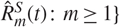 $\hat{R}_{m}^{S}(t)\colon m\geq1\}$ allows m to be selected so that fm(t) and Sm(t) achieve preset accuracies. The fact that expansion errors can be so effectively approximated using such saddlepoint methods makes the expansions much more valuable computationally than they would be otherwise. The approximations may also be used to correct the mth order expansions as fm(t) + R̂m(t) and
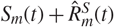 $S_{m}(t)+\hat{R}_{m}^{S}(t)$ to achieve even greater accuracy. Alternatively, the error terms may be computed by using numerical contour integration so that the corrected expansions can achieve even higher accuracy. This approach will be seen as easier that direct numerical inversion in the convergence domain since a much smaller term (just the error) is being numerically approximated.
If  $\mathcal{M}$ admits an infinite sequence of poles in which Re(bm) → +∞ as m → ∞, then the resulting infinite expansions f ∞ and S ∞ often provide convergent expansions for f and S. We show this happens in the computationally difficult case for the null distribution of Wilks’ likelihood ratio test in MANOVA in which
 $\mathcal{M}$ is not rational. This is a setting in which there is no exact expression in the literature for making p-value computations and in Section 2.7 we show how these new infinite expansions f ∞ and S ∞ can be expressed in terms of generalised hypergeometric functions. Various other examples are used to examine whether or not the infinite expansions f ∞ and S ∞ converge in the presence of convolutions and finite mixing.
The bulk of the discussion and numerical work concerns expansions for general compound distributions on (−∞, ∞) as well as for the Sparre Andersen and Cramér–Lundberg models with distributions on (0,∞). In the former general setting, we formulate very weak conditions in Theorem 3 and Corollary 3 for the existence of first-order expansions and also for the existence of new higher-order expansions, respectively. We also provide numerical examples to demonstrate the extraordinary accuracy of these expansions when b is a pole that assumes various orders. For the Sparre Andersen and Cramér–Lundberg models, where only first-order expansions have been previously considered, we again formulate very weak conditions for their existence in Theorem 4 and Corollary 4 and propose new higher-order expansions fm(t) and Sm(t) in Corollary 5. Connections are made to heavy-traffic approximations. In numerical examples such higher-order expansions are shown to provide accuracy which approaches that of exact computation.
1.2. Main contributions of the paper
The major point of this paper is that the computation of f and S from  $\mathcal{M}$ need not be based solely on values of
 $\mathcal{M}$ in its convergence domain. In fact, such computations can be better made by using values of
 $\mathcal{M}$ outside and in its analytic continuation in the following three ways.
The poles/essential singularities of
 $\mathcal{M}$ at b and further into its analytic continuation provide residue expansions as described above that are typically competitive or more accurate than traditional saddlepoint approximations which make use of values of $\mathcal{M}$ in its convergence domain.
Saddlepoint approximations implemented in the analytic continuation of
$\mathcal{M}$ often provide quite accurate approximations to the error integrals Rm(t) and $R_{m}^{S}(t)$ for the expansions in (1) and (3). This makes the expansions all the more important since it allows m to be chosen to achieve preset accuracy. When added to the expansions, they improve upon the accuracy of the expansions. For even greater accuracy, Rm(t) and $R_{m}^{S}(t)$ can be computed using simple numerical integration that makes a modest attempt at pursuing the steepest descent direction in the analytic continuation of $\mathcal{M}$.Inversion integrals for computing f (t) and S(t) necessarily have contours that begin in the convergence domain, but this does not mean that such contours should stay in the convergence domain to achieve the most efficient numerical inversion. Indeed, the most efficient computation allows such contours to be deformed (using Cauchy’s theorem) so that they make some attempt at pursuing the path of steepest descent which most often passes outside of the convergence domain for
$\mathcal{M}$ and into its analytic continuation.


The expansions in (1)–(3) only apply to the right tail as t → ∞. For the left tail, similar expansions for the density and cumulative distribution function (CDF) can be derived as t → − ∞. The theoretical development is given in Section 5.3 of Butler (Reference Butler2019a) and an example involving the compound distribution of Example 17 is given in Section 5.3.1.
Due to space limitations, analogous expansions and saddlepoint approximations for lattice distributions are presented elsewhere in Butler (Reference Butler2019b). A parallel but quite distinct theory results for lattice distributions which must also address periodicity of the mass function. Also, the MGFs are periodic and the inversion formulae involve finite contour integration and both of these facts lead to a parallel but different development of the expansions and saddlepoint approximations in the analytic continuation.
2. Expansions using the analytic continuation
Suppose that X is an absolutely continuous random variable on (−∞, ∞) with density f (t), distribution function F(t), and survival function S(t) = 1 − F(t). Define the MGF of X as  $\mathcal{M}(s) = \kE(\re^{sX})$ on the complex domain for which the expectation converges and suppose that this domain is {a < Re(s) < b} or {a ≤ Re(s) < b} for −∞ ≤ a ≤ 0 < b < ∞. Let the notation
 $\mathcal{M}( s) $ also denote the analytic continuation of the MGF to complex values s ∈ ℂ for which
 $\kE(\re^{sX})$ is not finite.
To ensure that the inversion theorem applies to density f (t) for t > 0, we assume that f (t) is locally of bounded variation for all t ∈ (0, ∞); see Doetsch (Reference Doetsch1974, Theorem 24.3) or Widder (Reference Widder1946, Chapter VI, Theorem 5a). The inversion theorem concerns the normalised version of density f (t) defined as  $\,\bar{\!f}(t)=\tfrac{1}{2}\{f(t^{+})+f(t^{-})\}$. In order to avoid distinctions between the two, we assume, without any loss in generality, that f (t) = f̄(t) is the normalised version at points for which it is not continuous.
2.1. Expansions for f(t) using pole b
The inversion formula for f (t) is
 \begin{equation}f(t)=\frac{1}{2\pi \im}\lim_{N\rightarrow\infty}\int_{b^{-}-\im N}^{b^{-} +\im N}\mathcal{M}(s)\re^{-st}\sd s,\end{equation}
where b − = b − ε with 0 < ε < b, and the integration is performed along the vertical line {Re(s) = b −} and within the convergence domain for  $\mathcal{M}$. Consider deforming this contour to allow integration along the vertical line {Re(s) = b + = b + ε} which is outside the convergence domain of
 $\mathcal{M}$ but still within its analytic continuation. If singularity b is an m-pole of
 $\mathcal{M}$ and the only singularity in {b ≤ Re(s) ≤ b +}, then we can use Cauchy’s residue theorem to relate the two integrals in terms of the residue of
 $\mathcal{M} (s)\re^{-st}$ at b > 0. If, apart from the pole at b,
 $\mathcal{M}$ possesses an analytic continuation to {Re(s) < b + ε 0} for ε 0 > ε, then Cauchy’s theorem can be applied to integration over the rectangular curve with the four corners b − ± iN and b + ± iN to give
 \begin{align}
f(t)&=\frac{1}{2\pi \im}\lim_{N\rightarrow\infty}\int_{b^{-}-\im
N}^{b^{-} +\im N}\mathcal{M}(s)\re^{-st}\sd s\nn\\
&=-\operatorname*{Res}\{\mathcal{M}(s)\re^{-st} ;\ b\}
+\frac{1}{2\pi \im}\lim_{N\rightarrow\infty}\bigg(
\int_{b^{+}-\im N}^{b^{+}+\im N}+\int_{b^{+}+\im N}^{b^{-}+\im
N}+\int_{b^{-}-\im N} ^{b^{+}-\im N}\bigg) \mathcal{M}(s)\re^{-st}\sd s.\nonumber\\
\end{align}
Subject to condition  $\mathcal{X}$ of Theorem 1 below, the last two integrals are negligible for large N so that (5) becomes
 \begin{equation}f(t)=-\operatorname*{Res}\{\mathcal{M}(s)\re^{-st};\ b\}+R_{1}(t),\end{equation}
with
 \begin{equation}R_{1}(t)=\re^{-b^{+}t}\frac{1}{2\pi}\int_{-\infty}^{+\infty}\mathcal{M} (b^{+}+\im y)\re^{-\im yt}\sd y,\end{equation}
where the improper integral is a principal-value integral. With the additional uniform integrability condition  $\mathcal{UI}$ of Theorem 1, then the integral in (7), whose contour lies outside the convergence domain of
 $\mathcal{M}$ but within the analytic continuation, can be made as small as o(1) as t → ∞. Thus, R 1(t) = o(e−b+t) as t → ∞ so (6) becomes
 \begin{equation}f(t)=\re^{-bt}\sum_{k=1}^{\mathfrak{m}}t^{k-1}\frac{({-}1)^{k}\beta_{-k}} {(k-1)!}+o(\re^{-b^{+}t}), \qquad t\rightarrow\infty.\end{equation}
Here, the residue has been determined by multiplying the Taylor expansion of e−st about s = b with the Laurent expansion of  $\mathcal{M}$ about b whose principal part is denoted as
 $\sum_{k=1}^{\mathfrak{m}}\beta _{-k}\break (s-b)^{-k}$. Sufficient conditions for the expansion in (8) are formalised in Theorem 1.
The leading term in this expansion is e−btt 𝔪−1(−1)𝔪β −𝔪/(𝔪 − 1)! and was given in Butler (Reference Butler2017, Proposition 1) with error o(t 𝔪−1e−bt) as t → ∞. By contrast, the use of Cauchy’s theorem determines the expansion in (8) with smaller-order error o(e−b +t), which should prove more accurate in numerical computations.
Before stating Theorem 1, it is worth emphasizing that the integral in (7) is not the Fourier inversion that leads to the tilted density fb+ (t) = eb +tf (t). For ε < 0,  $\mathcal{M} (b+\varepsilon+\im y)$, as a function of y, is the characteristic function of fb +ε (t) so that the inversion holds.
 \begin{equation}
f_{b+\varepsilon}(t)=\re^{(b+\varepsilon)t}f(t)=\frac{1}{2\pi}
\int_{-\infty }^{+\infty}\mathcal{M}(b+\varepsilon+\im y) \re^{-\im
yt}\sd y, \qquad\varepsilon\in({-}b,0),
\end{equation}
However, for ε ≥ 0, the identity in (9) does not hold because the integral is outside the convergence domain for  $\mathcal{M}(s)$.
Theorem 1. (Density expansions.) Suppose absolutely continuous X has density f (t) on support S⊆(−∞, ∞) which is locally of bounded variation for all t > 0. Also suppose that X has MGF  $\mathcal{M}$ with convergence boundary {s ∈ ℂ: Re(s) = b} with 0 < b < ∞. Subject to conditions
 $\mathcal{AC}, \mathcal{X}$ and
 $\mathcal{UI}$ on
 $\mathcal{M}$ below, the density has asymptotic expansion (8) as t → ∞ with error R 1(t) = o(e−b +t) as given in (7).
- {$\mathcal{AC}$. There exists ε 0 > 0 such that $\mathcal{M}$ can be analytically continued across its convergence boundary to {b ≤ Re(s) < b + ε 0}, save from an 𝔪-pole at b.
- $\mathcal{X}$. For some b + = b + ε with ε ∈ (0, ε 0),
\begin{equation}\max _{b \leq x \leq b^{+}}|\mathcal{M}(x+\mathrm{i} N)| \rightarrow 0, \qquad N \rightarrow \infty.\end{equation}
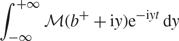
- $\mathcal{UI}$. For some T > 0, the principal-value integral
converges uniformly in t for t ≥ T.\begin{equation}\int_{-\infty}^{+\infty} \mathcal{M}\left(b^{+}+\mathrm{i} y\right) \mathrm{e}^{-\mathrm{i} y t} \mathrm{d} y\end{equation}


Proof. The proof follows from Doetsch (Reference Doetsch1974, Theorem 35.1) and details are given in Section 5.1.1 of Butler (Reference Butler2019a).
What is most notable about Theorem 1 is that its main assumptions  $\mathcal{AC}, \mathcal{X}$, and
 $\mathcal{UI}$ all concern
 $\mathcal{M}$ and not f. In many stochastic modelling applications,
 $\mathcal{M}$ is available but f is not, so such conditions are much simpler to check than conditions on f as were used in Butler (Reference Butler2017, Proposition 1). The only assumption made about f in Theorem 1 is that it is locally of bounded variation, i.e. for each t > 0, there is a small δt > 0 for which f is of bounded variation within (t − δt, t + δt). This is the weakest assumption under which the inversion formula (4) holds and is satisfied, for example, over sets for which f is finitely piecewise continuous.
The uniform integrability condition  $\mathcal{UI}$ can often be established by showing that M(b + + iy) is absolutely integrable in y. The next result follows directly from the Riemann–Lebesgue lemma (Feller (Reference Feller1971, p. 513)).
Lemma 1. If |M(b + + iy)| is integrable in y then  $\mathcal{UI}$ holds. If a δ > 0 and Y > 0 exist such that
 $\max_{b\,\leq\,x\,\leq b^{+}}| \mathcal{M}(x+\im y)| <c/|y|^{1+\delta}$ for |y| > Y and some c > 0, then conditions
 $\mathcal{X}$ and
 $\mathcal{UI}$ hold.
Example 1. (Minus log-beta.) The density of X = − ln{Beta (α, β)} provides an example in which the uniform integrability assumption  $\mathcal{UI}$ holds, but the absolute integrability in Lemma 1 may not. The MGF of X is
 $\mathcal{M}(s)=c\Gamma(\alpha -s)/\Gamma(\alpha+\beta-s)$ with c = Γ(α + β)/ Γ(α), and has the asymptotic order
 $|\mathcal{M}(x+\im y)|\sim c|y|^{-\beta}$ as y → ±∞ which is uniform over bounded values of x; see 5.11.9 of NIST DLMF (Reference Nist2014) in the references. If β ≤ 1 then absolute integrability does not hold; however,
 $\mathcal{UI}$ holds along with condition
 $\mathcal{X}$ as shown in Section 5.1.2 of Butler (Reference Butler2019a). Thus, from Theorem 1, the density of X has expansion f (t) = e−αtΓ(α + β)/{Γ(α)Γ(β)} + o(e−α +t) for all α > 0 and β > 0 and any α + ∈ (0, 1).
Theorem 1 can be extended to deal with the setting in which multiple poles lie along the convergence boundary {Re(s) = b}. The expansion is given as Equation (53) in Corollary 6 of Butler (Reference Butler2019a, Section 5.1.3).
Example 2. (Interfering poles.) Suppose that  $\mathcal{M}$ has 𝔪-poles at b and b ± yi, with respective mth order Laurent coefficients β −𝔪 = α 0,
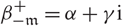 $\beta_{-\mathfrak{m}}^{+}= \alpha+\gamma \im,$, and
 $\beta_{-\mathfrak{m} }^{-}=\bar{\beta}_{-\mathfrak{m}}^{+}=\alpha-\gamma \im$, where the superscripts ± identify the associated pole b ± yi. Then expansion (53) in Corollary 6 of Butler (Reference Butler2019a) has the form
 \begin{equation}f(t)=\re^{-bt}\sum_{k=1}^{\mathfrak{m}}\frac{t^{k-1}(-1)^{k}c_{k} (t)}{(k-1)!}+o(\re^{-b^{+}t}),\end{equation}
where the term with the highest order has the coefficient
 c_{\mathfrak{m}}(t)=\beta_{-\mathfrak{m}} +\re^{-\im yt} \beta_{-\mathfrak{m}}^{+}+\re^{\im yt}\bar{\beta}_{-\mathfrak{m}}^{+}=\alpha_{0}+2\alpha\cos(yt)+2\gamma\sin(yt).
The periodicity of c 𝔪(t) is due to the presence of the complex conjugate pair of poles. If, instead, the poles at b ± yi are of lower order 𝔪1 < 𝔪 then c 𝔪(t) = β −𝔪 and the periodicity does not appear in the leading O(e−btt m−1) term, but rather in the lower-order O(e−btt 𝔪1−1) term.
2.2. Expansions for S(t) using pole b
An asymptotic expansion for S(t) also follows by using Cauchy’s theorem in the same manner as used in Theorem 1 under slightly weaker conditions.
Theorem 2. (Survival expansions.) Suppose absolutely continuous X with support in (− ∞, ∞) has the survival function S(t) and MGF  $\mathcal{M}$ with convergence boundary {s ∈ ℂ: Re(s) = b} with 0 < b < ∞. Subject to conditions
 $\mathcal{AC}$ and
 $\mathcal{X}$ of Theorem 1 as well as
 $\mathcal{UI}^{{S}}$ below on
 $\mathcal{M}$, then
 \begin{equation}S(t)=\sum_{k=1}^{\mathfrak{m}}S_{\text{G}(k,b)}(t)\frac{(-1)^{k}\beta_{-k} }{b^{k}}+R_{1}^{S}(t),\end{equation}
where  $\sum_{k=1}^{\mathfrak{m}}\beta_{-k}(s-b)^{-k}$ is the principal part of the Laurent expansion for
 $\mathcal{M}(s)$ at b, and SG (k,b) is the survival function of a gamma (k, b) distribution given by
 \begin{equation}\label{incomplete}S_{\text{G}(k,b)}(t)=\re^{-bt}\sum_{j=0}^{k-1}\frac{(bt)^{j}}{j!}.\end{equation}
with b + = b + ε, the error is
 \begin{equation}R_{1}^{S}(t)=\re^{-b^{+}t}\frac{1}{2\pi}\int_{-\infty}^{\infty}\frac {\mathcal{M}(b^{+}+\im y)}{b^{+}+\im y}\re^{-\im yt}\sd y=o(\re^{-b^{+}t}), \qquad t\rightarrow\infty.\end{equation}
 $\mathcal{UI}_{\rm m}$. For some T > 0, the principal-value integral
 \begin{equation*}\int_{-\infty}^{+\infty}\frac{\mathcal{M}(b^{+}+\im y)}{b^{+}+\im y}\re^{-\im yt}\sd y\end{equation*}
converges uniformly in t for t ≥ T.
Proof. The proof is the same as used in Theorem 1 but applied instead to the inversion formula of S(t). See Section 5.1.4 of Butler (Reference Butler2019a) for details.
If S 1(t) and f 1(t) are the expansions in (11) and (8), respectively, then  $S_{1}(t)=\int_{t}^{\infty}f_{1}(u)\sd u$ also the error terms in (13) and (7) are related by
 $R_{1} ^{S}(t)=\int_{t}^{\infty}R_{1}(u)\sd u$. Thus, expansion (11) could have been derived directly from Theorem 1 through the integration of (8) and subsequently showing that the error of o(e−b+t) is maintained after such integration. This is a legitimate argument but it also requires using the stronger condition
 $\mathcal{UI}$ of Theorem 1 rather than the weaker condition
 $\mathcal{UI}^{{\rm S}}$ of Theorem 2. Note also that no locally bounded variation assumption is needed for S(t), as there was for f (t), since S(t) has total variation 1.
Condition  $\mathcal{UI}^{{\rm S}}$ can often be shown to hold by using the following result.
Lemma 2. If 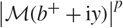 $\left| \mathcal{M} (b^{+}+\im y)\right| ^{p}$ is integrable for some p > 1 then
 $\mathcal{UI}^{{S}}$ of Theorem 2 holds. If δ > 0 and Y > 0 exist such that
 $\max_{b\leq x\leq b^{+}}\left| \mathcal{M}(x+\im y)\right| <c/|y|^{\delta}$ for |y| > Y and some c > 0, then conditions
 $\mathcal{X}$ and
 $\mathcal{UI}^{{S}}$ hold.
Proof. Use Hölder’s inequality so that
 \begin{equation}
\int_{-\infty}^{+\infty}\frac{| \mathcal{M}(b^{+}+\im y)|
}{| b^{+}+\im y| }\sd y\leq\bigg\{
\int_{-\infty}^{+\infty}| \mathcal{M}(b^{+}+\im y)| ^{p}\sd
y\bigg\} ^{1/p}\bigg\{ \int_{-\infty }^{+\infty}\frac{1}{|
b^{+}+\im y| ^{q}}\sd y\bigg\} ^{1/q}<\infty,
\end{equation}
where 1/p + 1/q = 1. The absolute integrability in (14) implies  $\mathcal{UI}^{{\rm S}}$.
Example 3. (Example 1 continued.) The MGF of X = − ln{Beta (α, β)} satisfies both conditions of Lemma 2 and SX(t) = e−αtΓ(α + β)/{αΓ(α)Γ(β)} + o(e−α+t).
When  $\mathcal{M}$ admits multiple poles along the convergence boundary {Re(s) = b}, then an expansion for S(t) is given in Equation (56) of Butler (Reference Butler2019a, Section 5.1.5, Corollary 7).
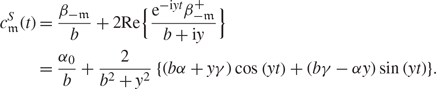
Example 4. (Example 2 continued.) The survival function expansion given in Butler (Reference Butler2019a, Equation (56)) has the same general form as (10) but with different coefficients  $\{c_{k}^{S}(t)\colon k=1,\ldots, \mathfrak{m\}}$ replacing {ck(t)}. After using (12) to expand S G(m,b) and S G(m,b+iy) in (56), then the leading term of order O(e−btt m−1) in S(t) is e−btt m−1(−1)mcSm(t)/(m − 1)!, with
 \begin{align*}
c_{\mathfrak{m}}^{S}(t) &=\frac{\beta_{-\mathfrak{m}
}}{b}+2{\mathrm{Re}}\Big\{ \frac{\re^{-\im
yt}\beta_{-\mathfrak{m}}^{+} }{b+\im y}\Big\}
\\
&=\frac{\alpha_{0}}{b}+\frac{2}{b^{2}+y^{2}}\left\{
(b\alpha+y\gamma)\cos\left( yt\right) +(b\gamma-\alpha y)
\sin(yt)\right\}\!.
\end{align*}
A tedious computation shows that  $c_{\mathfrak{m}}^{S}(t)=\int_{t}^{\infty }c_{\mathfrak{m}}(u)\sd u$, which is consistent with the fact that the survival expansion in Butler (Reference Butler2019a, Equation (56)) is the tail area for the density expansion in Butler (Reference Butler2019a, Equation (53)) when the latter expansion is valid. Note that the hazard function
 $f(t)/S(t)\sim c_{\mathfrak{m}}(t)/c_{\mathfrak{m}}^{S}(t)$ as t → ∞ and this ratio is a 2π/y-periodic function without a limit as discussed in Butler (Reference Butler2017, Section 3, Example 1).
2.3. Higher-order expansions using multiple poles
We now consider higher-order expansions for f (t) and S(t) related to poles of  $\mathcal{M}$ that lie further into the analytic continuation {Re(s) ≥ b}. The following alternative assumption is needed.
- $\mathcal{AC}_{{\rm m}}$. Either $\mathcal{M}$ has a monotone increasing sequence of distinct real poles b = b 1 < · · · < bm, where bj is an 𝔪j-pole, or it has a monotonic increasing sequence of complex conjugate pairs of poles denoted by b = b 1 < Re(b 2±) < · · · < Re(bm ±). Apart from these poles, $\mathcal{M}$ admits an analytic continuation into {b ≤ Re(s) < bm + ε 0}, with ε 0 > 0.


Nonreal poles must occur in complex conjugate pairs bj + and bj − = b̄j + due to the property that 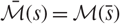 $\mathcal{\bar{M}}(s)=\mathcal{M} (\bar{s})$ for all s. Denote the principal part of the Laurent expansion of
 $\mathcal{M}$ about pole bj as
 $\sum_{k=1}^{\mathfrak{m}_{j}}\beta _{-k;j}(s-b_{j})^{-k}$.
Cauchy’s theorem is now used as in Theorems 1 and 2 to give an expansion in terms of the first m residues at {bk: k ≤ m} by displacing the contour integral from {Re(s) = b −} to 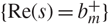 $\{{\mathrm{Re}} (s)=b_{m}^{+}\}$, where
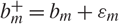 $b_{m}^{+}=b_{m}+\varepsilon_{m}$ with 0 < εm < ε 0.
Corollary 1. (Higher-order expansions.) Suppose that the density f (t) satisfies the conditions of Theorem 1 with conditions  $\mathcal{AC}_{{m}}, \mathcal{X}_{m},$, and
 $\mathcal{UI}_{m}$ on
 $\mathcal{M}$ replacing
 $\mathcal{AC}, \mathcal{X}$, and
 $\mathcal{UI}$.
- $\mathcal{X}_{{\rm m}}$. For some εm ∈ (0, ε 0), $\max_{b\,\leq\,x\,\leq b_{m}^{+}}\left| \mathcal{M}(x+\im N)\right| \rightarrow0$ as N → ∞.
- $\mathcal{UI}_{\rm m}$. For some T > 0, the principal-value integral $\int_{-\infty}^{+\infty}\mathcal{M}(b_{m} ^{+}+\im y)\re^{-\im yt}\sd y$ converges uniformly in t for t ≥ T.




Then,
 \begin{equation}f(t)=f_{m}(t)+R_{m}(t)\coloneqq\sum_{j=1}^{m}\re^{-b_{j}t} \sum_{k=1}^{\mathfrak{m}_{j} }t^{k-1}\frac{(-1)^{k} \beta_{-k;j}}{(k-1)!}+R_{m}(t),\end{equation}
where
 \begin{equation}R_{m}(t)=\re^{-b_{m}^{+}t}\frac{1}{2\pi}\int_{-\infty}^{+\infty} \mathcal{M} (b_{m}^{+}+\im y)\re^{-\im yt}\sd y=o(\re^{-b_{m}^{+}t}),\qquad t\rightarrow\infty.\end{equation}
Suppose that S(t) satisfies the conditions of Theorem 2 with conditions  $\mathcal{AC}_{m}$ and
 $\mathcal{X}_{m}$ on
 $\mathcal{M}$ replacing
 $\mathcal{AC}$ and
 $\mathcal{X}$, and the following assumption
 $\mathcal{UI}_{m}^{S}$ replacing
 $\mathcal{UI}^{S}$.
- $\mathcal{UI}_{{\rm m}}^{{\rm S}}$. For some T > 0, the principal-value integral $\int_{-\infty}^{+\infty} \mathcal{M} (b_{m}^{+}+\im y)(b_{m}^{+}+\im y)^{-1}\re^{-\im yt}\sd y$ converges uniformly in t for t


Then,
 \begin{equation}S(t)=S_{m}(t)+R_{m}^{S}(t)\coloneqq\sum_{j=1}^{m}\sum_{k=1}^{\mathfrak{m}_{j} }S_{\text{G}(k,b_{j})}(t)\frac{({-}1)^{k}\beta_{-k;j}}{b_{j}^{k}} + R_{m}^{S}(t),\end{equation}
where
 \begin{equation}R_{m}^{S}(t)=\re^{-b_{m}^{+}t}\frac{1}{2\pi}\int_{-\infty}^{+\infty} \frac{\mathcal{M}(b_{m}^{+}+\im y)}{b_{m}^{+}+\im y}\re^{-\im yt}\sd y = o(\re^{-b_{m}^{+} t}), \qquad t\rightarrow\infty,\end{equation}
and S G(k,bj) denotes the survival function of a gamma (k, bj) distribution as in (12).
If bj is rather a complex conjugate pair bj + and bj −, then (15) and (17) continue to hold but with the jth term summed over both j + and j −.
2.4. Expansions using essential singularities
If b and other finite singularities are isolated essential then similar residue expansions hold under the identical conditions used in Theorems 1 and 2 and Corollary 1. The formal statements of the corresponding results are identical apart from pole orders {mj} taking value ∞ so that residue sums are infinite. We provide two examples.
Example 5. (Compound Poisson distributions.) Here 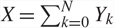 $X=\sum_{k=0}^{N}Y_{k}$, where N ~ Poisson (λ), {Yk: k ≥ 1} are independent and identically distributed (i.i.d.) with a meromorphic MGF
 $\mathcal{M}_{Y}(s)$, and Y 0 = 0 with probability 1. The MGF of X is
 $\mathcal{M}(s)=\exp[\lambda\{\mathcal{M}_{Y}(s)-1\}]$ and the poles of
 $\mathcal{M}_{Y}$ are isolated essential singularities of
 $\mathcal{M}$. Expansions for the conditional density and survival functions of X given X ≠ 0 make use of the residue expansions for these essential singularities. Unconditional expansions include the additional factor 1 − e−λ.
Example 6. (Noncentral χ 2(2m, λ).) The MGF is
 \begin{equation}\mathcal{M}(s)=\frac{1}{(1-2s)^{m}}\exp\Big\{ \frac{\lambda} {2}\Big( \frac{1}{1-2s}-1\Big) \Big\}\end{equation}
and  $b=\tfrac12$ is an essential singularity. From the form in (19) we see that this distribution is the convolution of a central χ 2(2m), which contributes the factor (1 − 2s)−m, and a compound Poisson with Poisson rate λ/2 and Y 1 ~ Exponential
 $(\tfrac12)$.
For m ≥ 2, the  $\mathcal{UI}$ condition holds due to Lemma 1; when m = 1,
 $\mathcal{UI}$ holds by an integration-by-parts argument as given in Butler (Reference Butler2019a, Section 5.1.6). The expansion errors in (7) and (13) are R 1(t) ≡ 0 ≡ R 1S(t) so the residue expansions are exact and take the form of infinite Poisson mixtures of well-known central χ 2 distributions of the form
 \begin{align}
f(t) & = -\operatorname*{Res}\Big\{\mathcal{M}(s)\re^{-st};\ \frac12
\Big\}=\sum _{k=0}^{\infty}\frac{\re^{-\lambda/2}}{k!}\Big(
\frac{\lambda}{2}\Big) ^{k}f_{\chi^{2}(2m+2k)}(t),\label{esssing}\end{align}
 \begin{align}S(t) & = -\operatorname*{Res}\Big\{ \frac{\mathcal{M}(s)}
{s}\re^{-st};\ \frac{1}{2}\Big\}
=\sum_{k=0}^{\infty}\frac{\re^{-\lambda/2}} {k!}\Big(
\frac{\lambda}{2}\Big) ^{k}S_{\chi^{2}(2m+2k)}(t). \label{esssing2}
\end{align}
Here fχ 2(2m+2k) and Sχ 2(2m+2k) are the density and survival functions of a central χ 2(2m + 2k) distribution. For details, see Butler (Reference Butler2019a, Section 5.1.6).
Alternatively, these expansions can be shown to hold for any real m > 0 by taking a Taylor expansion of the exponential term in  $\mathcal{M}$ about 0 and inverting the infinite sum term-by-term. Since the sum is infinite, justification for this must be based on Doetsch (Reference Doetsch1974, Theorem 30.1) which allows the inversion integral to be interchanged with the infinite sum. From this, we conclude that the identities in (20) and (21) hold for any real m > 0 and for a.e. t > 0.
2.5. Saddlepoint approximations in the analytic continuation
The expansion errors in (16) and (18) can be approximated by using either saddlepoint approximations or through numerical integration. In both integrals, if the integrand factor  $\mathcal{M}(s)\re^{-st}$ has another real pole at bm +1 > bm then a real saddlepoint ŝm ∈ (bm, bm +1) may exist to approximate the integrals. In such cases, saddlepoint approximations for Rm(t) and
 $R_{m}^{S}(t)$ are
 \begin{equation}R_{m}(t) \simeq\hat{R}_{m}(t)=\frac{1}{\sqrt{2\pi\mathcal{K}^{\prime \prime}(\hat{s}_{m})}\,}\exp\{\mathcal{K}(\hat{s}_{m})-\hat{s}_{m} t\},\end{equation}
 \begin{equation}R_{m}^{S}(t) \simeq\hat{R}_{m}^{S}(t)=\frac {1}{\sqrt{2\pi\{\mathcal{K}^{\prime\prime}(\mathfrak{\hat{s}}_{m} )+\mathfrak{\hat{s}}_{m}^{-2}\}}\,}\frac{1}{\mathfrak{\hat{s}}_{m}}\exp\{\mathcal{K}(\mathfrak{\hat{s}}_{m})-\mathfrak{\hat{s}}_{m}t\},\end{equation}
where  $\mathcal{K}(s)=\ln\mathcal{M}(s)$ and ŝm and
 $\mathfrak{\hat{s}}_{m}$ are the respective saddlepoint solutions to and in (bm, bm +1).
Proposition 1. (Existence of a saddlepoint in (bm, bm +1).) For the setting above in which consecutive poles bm < bm +1 are real, saddlepoints ŝm and  $\mathfrak{\hat{s}}_{m}$ exist in (bm, bm +1) if
 $\{\mathcal{M}(s)\colon s\in(b_{m},b_{m+1})\}$ is either a subset of (0, ∞) or a subset of (− ∞, 0).
An example of the setting for Proposition 1 is given in Figure 1 of Section 3.2.1. In such cases,  $\mathcal{M}(s)\re^{-st}$ achieves a minimum (maximum) value in (bm, bm +1) when
 $\mathcal{M}(s) 0 (<0)$. Also, in such cases,
 $\mathcal{K}(s)=\ln\mathcal{M}(s)$ is analytic on s ∈ (bm, bm +1) × (− δ, δ) ⊂ ℂ for sufficiently small δ > 0, so that
 $\mathcal{K}^{\prime}(s)-t$ must have a real zero for at least one ŝm ∈ (bm, bm +1). Such a point ŝm must therefore be a saddlepoint by the Cauchy–Riemann equations. This argument does not apply when
 $0\in\{\mathcal{M}(s)\colon s\in(b_{m},b_{m+1})\}$ This is because
 $\mathcal{K}(s)$ cannot be made analytic on (bm, bm +1) × (− δ, δ) since 0 is not in the domain of the ln function and an analytic branch of the multifunction
 $\ln\mathcal{M}(s)$ cannot be defined on (bm, bm +1) × (− δ, δ).
With this setup, the saddlepoint formulae in (22) and (23) can be derived as in Copson (Reference Copson1965, pp. 92–93) or Murray (Reference Murray1984, Chapter 3) based upon the steepest descents method. Both (22) and (23) presume that the saddlepoints are simple meaning that  $\mathcal{K}^{\prime\prime}(\hat{s}_{m})\neq0$ so the expressions are well defined as complex computations.
In many settings there is a unique real saddlepoint for  $\mathcal{M} (s)\re^{-st}$ in (bm, bm +1). This is the case for some simpler distributions such as the minus log-beta distribution (Examples 1 and 3), Wilks’ likelihood ratio statistic (Examples 7 and 8), the extreme value, logistic, and hyperbolic secant distributions (Example 10). This is also the case in a relatively complicated Cramér–Lundberg example (Example 19).
In settings where bm +1 is not real and is rather a complex conjugate pair of poles bm +1 and b̄m +1, then there may be multiple real or complex conjugate pairs of saddlepoints in {bm < Re(s) < Re(bm +1)}. This is illustrated in both the right and left tails of the compound distribution of Example 17 (see also Butler (Reference Butler2019a, Sections 5.3 and 5.3.1)) and in a Cramér–Lundberg example (Example 18). With multiple real or multiple complex conjugate pairs of saddlepoints, then a choice must be made between them when using (22) and (23) to approximate the inversion integrals for Rm(t) and  $R_{m}^{S}(t)$. We recommend the closest (pair) in terms of its real component. If one must deal with a complex conjugate pair of saddlepoints then such saddlepoints typically lie somewhere in the vicinity between bm and bm +1, and bm and b̄m +1, but not necessarily on straight lines as would happen when bm and bm +1 are both real poles. Also with a complex conjugate pair of saddlepoints, both saddlepoints are used in the approximation and the contour of the inversion integral must be deformable to pass along the path of steepest descent from each saddlepoint in the pair. Thus, in this case, (22) and (23) are applied by adding the contributions from both saddlepoints.
The saddlepoint approximation in (23) will be accurate without the need to apply the method of Bleistein (Reference Bleistein1966) to deal with the integrand factor  $(b_{m}^{+}+\im y)^{-1}$, since
 $b_{m}^{+}$ is not in the convergence domain of
 $\mathcal{M}$ and therefore well away from 0. If a value for
 $b_{0}^{+} \in(0,b)$ in (18) were chosen so it is in the convergence domain, then
 $R_{0}^{S}(t)=S(t)$ and the approximation in (23) using a saddlepoint in (0, b) would not be as accurate as the Lugannani and Rice (Reference Lugannani and Rice1980) saddlepoint approximation for S(t), which is based upon the Bleistein method.
If  $\mathcal{M}$ is analytic on {Re(s) > bm} then deforming the contour integral further to the right cannot change the errors Rm(t) and
 $R_{m}^{S}(t)$. Also, there may not be any saddlepoints in this region to approximate these errors. An example is the random variable −ExV * Exp (1), where ExV is an extreme value distribution with MGF Γ(1 − s). The convolution distribution has MGF Γ(1 + s)/(1 − s) with poles {…, −2, −1, 1} and f 1(t) = e−t = S 1(t) have errors R 1(t) = −e−et (1 + e−t) and
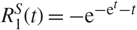 $R_{1}^{S}(t)=-\re^{-\re^{t} -t}$. In examples for which
 $\mathcal{M}$ is meromorphic with only a finite number of poles outside of {a < Re(s) < b}, then
 $\mathcal{M}$ is rational and such errors are 0. For example, with poles only at an < · · · < a 1 < 0 < b < · · ·< bm, then f (t) = fm(t) and S(t) = Sm(t) for t > 0.
2.6. Examples
The expansions and saddlepoint approximations together can provide more accurate approximations to f (t) and S(t) than the individual methods used separately as seen in the next example.
Example 7. (Wilks’ likelihood ratio statistic,  $\mathcal{M}$ rational.) The likelihood ratio statistic Λk,p,n in MANOVA has null distribution, with ai = n − i+ 1 and all beta variates independent. Here, k denotes dimension, p is the degrees of freedom for hypothesis, and n is the degrees of freedom for error. Taking k = 3, p = 6, and n = 7, then the MGF for − ln Λ3,6,7 is
 \begin{align}
\mathcal{M}(s) & = c\,\prod_{\im=1}^{3}\frac{\Gamma\{(8-\im)/2-s\} }{\Gamma\{(14-\im)/2-s\} }\nonumber\\
& = c\big\{ \big( \tfrac52-s\big) \big( 3-s\big) \big(\tfrac72-s\big) ^{2}\big( 4-s\big) \big( \tfrac92-s\big)^{2}\big( 5-s\big) \big(\tfrac{11}{2}-s\big) \big\} ^{-1}
\end{align}
where 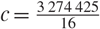 $c=\tfrac{3\,274\,425}{16}$ and
 $s<a_{3}/2=\tfrac52=b$. The MGF has seven poles ranging from
 $\tfrac52$ to
 $\tfrac{11}{2}$ in increments of
 $\tfrac12$ with 1-poles at
 $\tfrac52$, 3, 4, 5, and
 $\tfrac{11}{2}$ and 2-poles at
 $\tfrac72$ and
 $\tfrac92$. This rational form for
 $\mathcal{M}$ occurs whenever either p is even or k is even with the latter setting following from the fact that Λk,p,n and Λp,k,p+n−k have the same distribution. From the rational form in (24), the exact density/survival functions can be easily computed through partial fraction inversion. This approach can be shown to be equivalent to that used by Schatzoff (Reference Schatzoff1966) who worked in the time domain by successively convoluting log-beta densities.
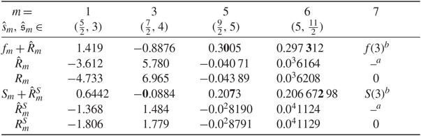
Various density and survival approximations, fm(3) + R̂m(3) and 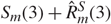 $S_{m}(3)+\hat{R}_{m}^{S}(3)$, for f (3) = 0.297 316 and S(3) = 0.206 673 47 where m denotes the number of residues included. The boldface digit indicates the last ‘accurate’ digit or the last digit in agreement with the exact result when both are rounded to the same number of digits. Also shown are saddlepoint approximations R̂m(3) and
 $\hat{R}_{m}^{S}(3)$ for errors Rm(3) and
 $R_{m}^{S}(3)$, respectively, along with exact (numerically integrated) computations for these errors.
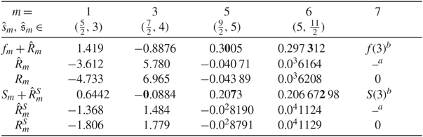
a Indicates that R̂m or  $\hat{R}_{m}^{S}$ is undefined.
b Indicates that the seven residue sum is exact.
In Table 1 we show the approximations of Corollary 1 for f (3) = 0.297 316 and S(3) = 0.206 673. The entries demonstrate that a sufficient number m of residue terms are needed in order for the asymptotic expansions to achieve an accurate approximation. This should have been expected in this example from the nature of the asymptotic expansion since the poles are spaced relatively close together with increments of  $\tfrac12$. The entries for saddlepoint error approximations R̂m(3) and
 $\hat{R}_{m}^{S}(3)$ provide guidance about the expansion error and appear quite useful in determining the value of m needed to ensure sufficient accuracy. Both approximations need to sum residues to at least the 2-pole at m = 5 in order to achieve any kind of accuracy. Inaccuracy for m ≤ 4 occurs because successively added residue terms fluctuate in sign and magnitude. This is caused by quite large residues that are not adequately dampened by the gradually diminishing exponential values {exp (− bj t)} using poles {bj} in increments of
 $\tfrac12$ which are not well spaced.
Saddlepoint density and Lugannani and Rice (Reference Lugannani and Rice1980) survival approximations applied in the convergence strip  $\{s<\tfrac52\}$ of the MGF lead to the values 0.2984 and 0.2061, respectively, where the boldface digits indicate the last ‘accurate’ digit or the last digit in agreement with the exact result when both are rounded to the same number of digits. These approximations attain remarkable accuracy which is slightly better than expansions to m = 5 and exceeded only by using m = 6 residues. When term m = 7 is included, the expansions are exact.
Example 8. (Wilks’ likelihood ratio statistic,  $\mathcal{M}$ is not rational.) Consider the case in which both p and k are odd. This is the setting in which there are no exact computational procedures (however, see Section 2.7 below). We take k = 3, p = 5, and n = 7 so the MGF for − ln Λ3,5,7 is
 \begin{equation}\mathcal{M}(s)=c_{1}\,\frac{1}{\left( 5/2-s\right) \left( 3-s\right)\left( 7/2-s\right) ^{2}\left( 4-s\right) \left( 9/2-s\right) ^{2}}\times\frac{\Gamma(11/2-s)}{\Gamma(6-s)},\end{equation}
where  $c_{1}=30240/\sqrt{\pi}$ There are poles at
 $\tfrac52$, 3,
 $\tfrac72$, 4,
 $\tfrac92, \tfrac{11}{2}$ with saddlepoints in between; however, above
 $\tfrac{11}{2}$ there are no saddlepoints. At
 $\tfrac{11}{2}$ and above there are simple poles at
 $\tfrac{11}{2},\tfrac{13}{2},\ldots$, but
 $\mathcal{M}(s)$ is monotone decreasing in between each pair of poles with
 $\infty=\mathcal{M}\{(k-\tfrac12)^{+}\}> \mathcal{M}\{(k+\tfrac12)^{-}\}=-\infty$ for k ≥ 6, so Proposition 1 does not hold. Since
 $\Gamma(\tfrac{11}{2}-s)/\Gamma (6-s)\sim1/\sqrt{-s}$ when Re(s) is fixed and Im (s) → ∞, then
 $|\mathcal{M}(s)|= O(|s|^{-{15}/{2}} )$; thus, conditions
 $\mathcal{AC}_{\rm m}, \mathcal{X}_{\rm m}$, and
 $\mathcal{UI}_{\rm m}$ of Corollary 1 hold for all m ≥ 1.
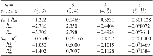
Various density and survival approximations for f (2.7) = 0.301 133 and S(2.7) = 0.201 400 8 where m denotes the number of residues included. See Table 1 for further description.
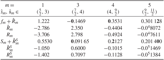
In Table 2 we show the accuracy that can be achieved when using the expansions and saddlepoint approximations to determine f (2.7) = 0.301 133 and S(2.7) = 0.201 400 8. Five terms (m = 5) are needed to stabilise the expansion but five terms result in 5 digit accuracy (after rounding) for both density and survival approximations. For comparison, the saddlepoint density and Lugannani and Rice (Reference Lugannani and Rice1980) survival approximations are 0.3028 and 0.2009, respectively, with 2 and 3 digit accuracy (after rounding); this is considerably better than the four term expansion but much less accurate than using five residue terms.
In both examples, the saddlepoint error approximations R̂m and  $\hat{R}_{m}^{S}$ make it very clear which values of m provide adequate and inadequate expansions. This is an important aspect of the methods if they are to ensure a specified accuracy particularly when poles are not well spaced as occurs in these two examples.
2.7. Expansions using an infinite number of poles
If  $\mathcal{M}$ admits an infinite sequence of increasing poles b = b 1 < b 2 < · · · and Corollary 1 can be assumed to hold for all m = 1, 2, …, then we obtain infinite expansions for f (t) and S(t) which we can denote as
 \begin{equation}%\label{dwig}
f(t)\approx f_{\infty}(t),\qquad S(t)\approx S_{\infty}(t).\nonumber
\end{equation}
The proper meaning for these expansions is that Corollary 1 holds for each m < ∞. The infinite sums f ∞ (t) and S ∞(t) may or may not be pointwise convergent and if so, may or may not converge to f (t) and S(t). We formalise the conditions for equality in the next result whose proof is based on Cauchy’s theorem.
Corollary 2. Suppose that Corollary 1 holds for all m = 1, 2, … Then
(a) f ∞(t) is convergent and f (t) = f ∞(t) if and only if there exists a sequence {εm} such that Rm(t) → 0 as m → ∞;
(b) S ∞(t) is convergent and S(t) = S ∞(t) if and only if there exists a sequence {εm} such that
$R_{m}(t)\rightarrow0$ as m → ∞;(c) if (a) holds then (b) holds.

Proof. Only (c) requires comment. If f(t) = f ∞(t) then S(t) = S ∞(t) follows from Fubini’s theorem.
The condition Rm(t) → 0 as m → ∞ is an existence condition for a particular sequence of vertical contours  $\{{\mathrm{Re}}(s)=b_{m}^{+}=b_{m}+\varepsilon_{m}\}$ such that Rm(t), the integral over this vertical line, converges to 0 as m → ∞. It is not necessary that this holds for all possible sequences. Typically
 $b_{m}^{+}\rightarrow\infty$, so in relatively straightforward cases Rm(t) → 0 if it can be shown that
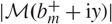 $|\mathcal{M}\mathbf{(}b_{m}^{+}+\im y)|$ is uniformly integrable for sufficiently large values of m. Examples where these series correctly converge to f (t) and S(t) are now given.
Example 9. (Example 1 continued.) For integer-valued β ∈ {1, 2, …}, the minus log-beta MGF  $\mathcal{M}(s)=\Gamma (\alpha+\beta)\Gamma(\alpha-s)/\{\Gamma(\alpha) \Gamma(\alpha+\beta-s)\}$ is a rational function with β simple poles so an exact finite expansion is easily determined. For β ∉ {1, 2, …},
 $\mathcal{M}$ has simple poles at s = α, α + 1, … and the exact density and survival functions are recovered from the infinite expansion of residues; see Section 5.1.7 of Butler (Reference Butler2019a).
Example 10. (Extreme value, logistic, and hyperbolic secant(θ).) These distributions have respective MGFs Γ(1 − s), Γ(1 + s)Γ(1 − s), and cos(θ)/ cos(θ + s) for θ ∈ (− π/2, π/2). All three distributions satisfy all parts of Corollary 2 and the details are given in Section 5.1.7 of Butler (Reference Butler2019a).
Example 11. (Example 8 continued.) From (25), the MGF has the form  $\mathcal{M}(s)=\mathcal{M}_{5}(s)\times\Gamma(11/2-s)/\Gamma(6-s)$, where
 $\mathcal{M}_{5}(s)$ contributes the first 5 poles which lead to the term f 5(t) based on the associated residues. The latter factor
 $\Gamma(\frac{11}{2}-s)/\Gamma(6-s)$ has an infinite sequence of simple poles at
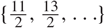 $\{\frac{11}{2},\frac{13}{2},\ldots\}$, which contributes an infinite sum of residues. All conditions of Corollary 2 are shown to hold in Section 5.1.7 of Butler (Reference Butler2019a). After simplification, the residue summation becomes the convergent hypergeometric expansion in
 \begin{equation}f(t)=f_{\infty}(t)=f_{5}(t)-\frac{672}{\pi}\re^{-(11/2)t}\,_{4}F_{3}\Big(\frac {1}{2},1,1,\frac{3}{2};\ 3,\frac{7}{2},4;\ \re^{-t}\Big).\nonumber\end{equation}
The exact survival function has S(t) = S ∞(t), which is also expressible in terms of 4F 3 hypergeometric functions. Thus, Corollary 2 provides exact expressions for the density and survival functions of Wilks’ likelihood ratio statistic in the intractable setting where k and m are odd-valued, which is the setting in which no exact results have previously been derived. General expressions can be derived for arbitrary odd values of k and m and a computational algorithm is under development to make such computations simple in the general case. Similar infinite residue expansions can be developed for all the other log-likelihood ratio test statistics in normal theory MANOVA as they involve sums of independent log-beta distributions with structure similar to this example; see Anderson (Reference Anderson2003, Chapters 9 and 10).
2.8. Convolutions and finite mixtures
For convolution distributions, the infinite expansions in Corollary 2 may or may not converge as seen in the next three examples. The first two examples convolve a density that has a convergent expansion with a density whose MGF is an entire function.
Example 12. (ExV * Normal.) The convolution of an extreme value and an independent normal distribution leads to divergent sums for both f ∞(t) and S ∞(t). The MGF is  $\mathcal{M}(s)=\Gamma(1-s)\exp(s^{2}/2)$ and has simple poles at j = 1, 2, … with
 $\operatorname*{Res}(\mathcal{M};\,j)=(-1)^{j} /(j-1)!\times\exp(j^{2}/2)$. In f ∞(t), the residue factor exp (j 2/2) from the normal term dominates e−jt for all t so f ∞(t) and also S ∞(t) diverge. Here,
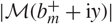 $|\mathcal{M} (b_{m}^{+}+\im y)|$ is integrable (see Butler (Reference Butler2019a, Section 5.1.8)) but not uniformly integrable in m while
 $\mathcal{AC}_{\rm m}, \mathcal{X}_{\rm m}, \mathcal{UI}_{\rm m}$, and
 $\mathcal{UI}_{\rm m}^{\rm S}$ hold for all m. Thus, Corollary 1 applies for all m and the divergence of f ∞(t) is due to the nonexistence of a sequence {εm} for which Rm(t) → 0 as m → ∞. Using m = 5 terms, f 5(1.7) = 2.0506 with f (1.7) = 0.1697 and R̂ 5(1.7) = −1.6202 with R 5 = −1.8813. The saddlepoint sequence { R̂m} also captures this divergence since R̂ 6(1.7) = 16.35 with R 6(1.7) = 18.89.
Example 13. (ExV * Uniform (0, 1).) Both f ∞(t) and S ∞(t) converge to f (t) and S(t), respectively, if we convolve an extreme value distribution with an independent uniform on (0, 1). The  $MGF\,\mathcal{M}(s)=\Gamma (1-s)(\re^{s}-1)/s$ has
 $\operatorname*{Res}(\mathcal{M};\,j)=(-1)^{j} /(j-1)\times(\re^{\,j}-1)/j$ and now factor ej − 1 does not overwhelm e−jt when summed over j as occurred in Example 12. See Butler (Reference Butler2019a, Section 5.1.8) for more details.
Example 14. (General convolution.) Let the MGFs  $\mathcal{M}_{1}(s)$ and
 $\mathcal{M}_{2}(s)$ both satisfy Corollary 2. Then the convolution density for
 $\mathcal{M}_{1}(s)\mathcal{M}_{2}(s)$ may also admit a convergent infinite residue expansion about the combined set of poles for
 $\mathcal{M}_{1}(s)$ and
 $\mathcal{M}_{2}(s)$ denoted as {bn}. If bn → ∞ then a sufficient condition is the existence of an N and a sequence {εn} such that
 $b_{n}^{+}=b_{n} +\varepsilon_{n}\in(b_{n},b_{n+1}),$, and
 $|\mathcal{M}_{1}(b_{n}^{+}+\im y))|$ and
 $|\mathcal{M}_{2}(b_{n}^{+}+\im y))|$ are uniformly integrable for n > N. When
 $\mathcal{M}_{1}(s)$ and
 $\mathcal{M}_{2}(s)$ share common poles, then this expansion depends on coefficients from the analytic portions of the Laurent expansions for
 $\mathcal{M}_{1}(s)$ and
 $\mathcal{M}_{2}(s)$ at these common poles. An example satisfying this sufficient condition and sharing poles is given in Butler (Reference Butler2019a, Section 5.1.8) in which X and Y have MGFs Γ(1 − s) and Γ(1 − 2s), and the density of X + Y is derived as an infinite convergent expansion.
Example 15. (Laplace distribution.) This distribution is the difference of two independent Exponential (1) variables and it provides an example in which there are poles at ±1 and for which expansions exist in both the right and left tails. If the appropriate expansions are used in either tail then f 1(t) = e−t/2 for t > 0 in the right tail and fL 1(t) = et/2 for t < 0 is the expansion in the left tail. Together they reproduce f (t) = e−|t|/2 for t ∈ (− ∞, ∞). Also left-tail expansion F 1(t) = et/2 for t ≤ 0 and S 1(t) = e−t/2 for t ≥ 0, so all agree with their exact counterparts. This example reinforces the point that the expansions should only be used in their appropriate tails.
If all the components of a finite mixture distribution admit convergent expansions then a weighted sum of these expansions provides the expansion for the mixture distribution and f ∞(t) = f (t) and S ∞(t) = S(t). If, however, a component distribution lacks such an expansion then f ∞(t) and S ∞(t) can converge but perhaps to the wrong density/survival function.
Example 16. (Mixture of ExV and Uniform (0, 1).) Consider a finite mixture of ExV and a uniform distribution on (0, 1) using equal weights. The MGF is  $\mathcal{M} (s)=\{\Gamma(1-s)+(\re^{s}-1)/s\}/2$ and
 $\operatorname*{Res}\{\mathcal{M}% (s);\,j\}=({-}1)^{j}/(j-1)!/2=\operatorname*{Res}\{\Gamma(1-s)/2;\,j\}$ so that f ∞(t) = f ExV(t)/2. This, however, differs from f (t) = { f ExV(t) + 1{0<t<1}}/2 on the interval {0 < t < 1}, where the uniform has its support. Likewise, S ∞(t) = S ExV(t)/2 = [S ExV(t) + {1{t<1} −t 1{0<t<1}}]/2 = S(t). Conditions
 $\mathcal{AC}_{\rm m}, \mathcal{X}_{\rm m}, \mathcal{UI}_{\rm m},$, and
 $\mathcal{UI}_{\rm m}^{\rm S}$ hold for all m, but a sequence of {εm} cannot be found for which Rm(t) → 0 as m → ∞.
The difficulty in Example 16 is that the residue expansion recognises addend Γ(1 − s)/2 but not addend (es − 1)/(2s), which has no finite singularities. In the density inversion, addend 1{0<t<1} /2 as a part of f (t) remains in the error term Rm(t) for all m since, by Cauchy’s theorem, the corresponding addend (es − 1)/s}/2 in  $\mathcal{M}(s)$ is an entire function. This phenomenon occurs whenever an addend in
 $\mathcal{M}(s)$ is an entire function and demonstrates that such residue expansions should not be used with mixture distributions in such instances.
3. Compound distributions as infinite mixtures
In insurance mathematics a ruin amount R is often a compound distribution 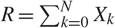 $R=\sum_{k=0}^{N}X_{k}$, where N ∈ {0, 1, …} has a weighting distribution with probability generating function (PGF)
 $\mathcal{P} (z)=\sum_{k=0}^{\infty}p(k)z^{k}$ which is convergent on {z ∈ ℂ: |z| < r} for r > 1. Suppose that X 0 puts mass 1 at 0 and {Xk: k ≥ 1} are i.i.d. absolutely continuous claim amounts with support in (−∞, ∞). Let X 1 have density fX(t) and MGF
 $\mathcal{M}_{X}(s)$ which converges in the right half of the complex plane on {0 ≤ Re(s) < c} or {0 ≤ Re(s) ≤ c} with 0 < c ≤ ∞. When
 $\mathcal{M}_{X}(c)<\infty$, then suppose that
 $r<\mathcal{M}_{X}(c)$ so that in all settings there is a unique root b to
 $\mathcal{M}_{X}(s)=r$ such that b ∈ (0, c). Ruin R has a compound distribution with MGF
 $\mathcal{P}\{\mathcal{M}_{X}(s)\}$ which converges on {0 ≤ Re(s) < b} in the right half of the complex plane. The special case in which
 $\mathcal{P}(z)$ is a geometric (1 − 1/r) PGF leads to an infinite mixture distribution with geometric weights and includes the Cramér–Lundberg and Sparre Andersen risk models as described in Feller (Reference Feller1971, Chapter XI.7) and considered in Section 4. The case in which
 $\mathcal{P}(z)$ is negative binomial (n, 1 − 1/r) was considered by Embrechts et al. (Reference Embrechts, Maejima and Teugels1985) and Sundt (Reference Sundt1982).
In the general compound distribution setting, we now give new first-order expansions for the density and survival functions of the ruin amount R with support S ⊆ (−∞, ∞). The proof is relegated to Section 5.2.1 of Butler (Reference Butler2019a). The following conditions are needed on fX(t) and  $\mathcal{M} _{X}(b+\varepsilon_{1}+s)$, the transform for the unnormalised tilted density e(b+ε 1)tf X(t) for some ε 1 > 0.
- $\mathcal{AI}_{\rm p}^{{\rm CD}}$. For some ε 1 ∈ (0, c − b), $|\mathcal{M}_{X}(b+\varepsilon_{1}+\im y)|^{p}$ is integrable in y for some integer p ≥ 1.
- $\mathcal{UI}^{\rm CD}$. If p ≥ 2 then, for k = 1, …, p − 1, there exists Tk > 0 such that the principal-value integral $\int_{-\infty}^{\infty}\mathcal{M}_{X} (b+\varepsilon_{1}+\im y)^{k}\re^{-\im ty}\sd y$ converges uniformly in t for t > Tk.




A sufficient condition for both  $\smash{\mathcal{AI}_{\rm p}^{\rm CD}}$ and
 $\mathcal{UI}^{\rm CD}$ to hold is that
 $|\mathcal{M}_{X}(b+\varepsilon_{1}+\im y)|$ is integrable in y for some ε 1 ∈ (0, c − b). Necessary conditions for such absolute integrability are that fX(t) is continuous and bounded (Feller (Reference Feller1971, Chapter XV.3, Theorem 3)). The exponential density, for example, is neither continuous nor does it satisfy this absolute integrability condition, but it does satisfy the weaker stated conditions
 $\mathcal{AI}_{\rm p}^{\rm CD}$ and
 $\mathcal{UI}^{\rm CD}$ as well as the next very weak condition.
- $\mathcal{BV}^{\rm CD}$. Integer q ≥ 1 exists such that $f_{X}^{(\ast q)}(t)$, the q-fold convolution of fX, has bounded variation on (−∞, ∞). If q ≥ 2 then, for k = 1, …, q − 1, assume that $f_{X}^{(\ast k)}(t)$ is locally of bounded variation for all t ∈ S ∩ (0, ∞).


Theorem 3. (Density/survival expansions for compound distributions.) Let  $\mathcal{P}(z)$ and
 $\mathcal{M}_{X}(s)$ be as described above. Suppose that the convergence bound r > 1 is an m-pole of
 $\mathcal{P}(z)$ which is analytic on {z ∈ ℂ: |z| ≤ r} apart from its pole at r.
If conditions  $\mathcal{AI}_{p}^{CD}$,
 $\mathcal{UI}^{CD}$, and
 $\mathcal{BV}^{CD}$ hold, then there exists an ε ∈ (0, ε 1) sufficiently small such that the density of R has the expansion
 \begin{equation}f_{R}(t)=\re^{-bt}\sum_{k=1}^{\mathfrak{m}}t^{k-1}\frac{({-}1)^{k}\beta_{-k}}{(k-1)!}+o(\re^{-(b+\varepsilon)t}), \qquad t\rightarrow\infty,\end{equation}
with
 \begin{equation}\beta_{-k}=\sum_{j=0}^{\mathfrak{m}-k}\frac{\rho_{-k-j}}{j!}\frac{\rd^{j}}{\rd s^{j}}\Big( \frac{1}{\{\mathcal{N}(s)\}^{k+j}}\Big) _{s=b},\end{equation}
where  $\sum_{k=1}^{\mathfrak{m}}\rho_{-k}(z-r)^{-k}$ specifies the principal part of the Laurent expansion for
 $\mathcal{P}(z)$ at r,
 $\mathcal{N}(s)=\{\mathcal{M}_{X}% (s)-r\}/(s-b)$,
 $\mathcal{N}(b)=\mathcal{M}_{X}^{\prime}(b)$, and
 $\smash{\mathcal{N}^{(j)}(b)=\mathcal{M}_{X}^{(j+1)}(b)/(j+1)}$.
Assuming that only condition  $\mathcal{AI}_{p}^{CD}$ holds, there exists an ε ∈ (0, ε 1) sufficiently small such that the survival function of R has the expansion
 \begin{equation}S_{R}(t)=\sum_{k=1}^{\mathfrak{m}}S_{\text{G}(k,b)}(t)\frac{(-1)^{k}\beta_{-k}}{b^{k}}+o(\re^{-(b+\varepsilon)t}),\qquad t\rightarrow\infty.\end{equation}
Proof. The theorem follows from Theorems 1 and 2 if the conditions for these theorems can be shown to hold. Such theorems cannot be expected to hold for R directly because it has a point mass at 0 with probability p(0). This leads to p(0) as the leading term in a Taylor expansion for  $\mathcal{P}\{\mathcal{M}_{X}(s)\}$ so that conditions
 $\mathcal{X}$ and
 $\mathcal{UI}$ of Theorem 1 typically do not hold. We work instead with random variable R +, defined as R given that R ≠ 0, which has an absolutely continuous distribution on (− ∞, ∞) with MGF
 \begin{equation}\mathcal{M}_{R^{+}}(s)=\frac{\mathcal{P}\{\mathcal{M}_{X}(s)\}-p(0)}{1-p(0)}.\end{equation}
The conditions of Theorem 3 ensure that Theorems 1 and 2 can be applied to  $\mathcal{M}_{R^{+}}(s)$; the details are relegated to Butler (Reference Butler2019a, Section 5.2.1).
In Theorem 3 we state that expansions (26) and (28) exist for a sufficiently small ε ∈ (0, ε 1). If, however,  $\mathcal{M}_{R^{+}}$ can be analytically continued to {Re(s) < b + ε 0} for ε 0 > 0 apart from its pole at b, then these first-order expansions may hold to order o{e−(b+ε)t} for any ε ∈ (0, ε 0). Corollary 8 of Butler (Reference Butler2019a, Section 5.2.2) provides the modest conditions needed for this to hold.
Conditions  $\mathcal{AI}_{\rm p}^{\rm CD}$,
 $\mathcal{UI}^{\rm CD}$, and
 $\mathcal{BV}^{\rm CD}$ represent the weakest conditions under which it has been possible to prove Theorem 3. Such weak conditions allow the density of X to be unbounded and for
 $|\mathcal{M}_{X}(b+\varepsilon_{1}+\im y)|$ to not be integrable. For example, consider the gamma (α, c) distribution with α ∈ (0, 1]. Any such distribution satisfies
 $\mathcal{AI}_{\rm p}^{\rm CD}$ and
 $\smash{\mathcal{UI}^{\rm CD}}$ since integrand {1 − (b + ε 1 + iy)/c}−αke−ity is uniformly integrable in y for all k ≥ 1 (using an integration-by-parts argument) and absolutely integrable for k > 1/α. Any such gamma (α, c) density also satisfies condition
 $\mathcal{BV}^{\rm CD}$ with q = ⌈1/α⌉ for S = (0, ∞).
3.1. Higher-order expansions
If  $\mathcal{M}_{R}$ is a meromorphic function in its analytic continuation {Re(s) ≥ b}, then higher-order expansions can be computed subject to the conditions below. In order to simplify the resulting expansions, we assume simple poles in
 $\mathcal{AC}_{\rm m}^{\rm CD}$ below, which result by assuming that
 $\mathcal{P}$ admits only one simple pole at r.
- $\mathcal{AC}_{\rm m}^{\rm CD}$. The function $\mathcal{M}_{R}$ admits a sequence of simple real poles b = b 1 < · · · < bm or a complex conjugate sequence of simple poles for which b = b 1 < Re(b 2±) < · · · < Re(bm ±). Apart from these poles, $\mathcal{M}_{R}$ can be continued analytically to {b ≤ Re(s) < bm + ε 0} for some ε 0 > 0.
- $\mathcal{AI}_{\rm mp}^{\rm CD}$. There exists εm ∈ (0, ε 0) and integer p ≥ 1 such that $|\mathcal{M}_{X}(b_{m}^{+}+\im y)|^{p}$ is integrable in y for $b_{m}^{+}=b_{m}+\varepsilon_{m}$. If $b_{m}^{+}>c$ then $\max_{c\,\leq\,x\,\leq b_{m}^{+}}| \mathcal{M} _{X}(x+iN)| \rightarrow0$ as N → ∞.
- $\mathcal{UI}_{\rm m}^{\rm CD}$. If p ≥ 2 in condition $\mathcal{AI}_{\rm mp}^{\rm CD}$ then, for k = 1, …, p − 1, there exists Tk > 0 such that the principal-value integral $\int_{-\infty}^{\infty}\mathcal{M}_{X}(b_{m}^{+} +\im y)^{k}\re^{-\im ty}\sd y$ converges uniformly in t for t > Tk.



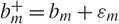





Corollary 3. (Higher-order expansions for compound distributions.) Let  $\mathcal{P}(z)$ and
 $\mathcal{M}_{X}(s)$ be as described in Theorem 3.
If fX satisfies the bounded variation conditions of  $\mathcal{BV}^{CD}$, and
 $\mathcal{M}_{R}$ and
 $\mathcal{M}_{X}$ satisfy conditions
 $\mathcal{AC}_{m}^{CD}$,
 $\mathcal{AI}_{mp}^{CD}$, and
 $\mathcal{UI}_{m}^{CD}$ above with simple real poles, then
 \begin{equation}f_{R}(t) = f_{m}(t)+R_{m}(t)\coloneqq\sum_{j=1}^{m}\re^{-b_{j}t} \frac{-\rho_{-1}}{\mathcal{M}_{X}^{\prime}(b_{j})}+R_{m}(t),\qquad t\rightarrow\infty,\end{equation}
 \begin{equation}R_{m}(t) = \frac{1-p(0)}{2\pi}\re^{-b_{m}^{+}t}\int_{-\infty}^{\infty}\mathcal{M}_{R^{+}}(b_{m}^{+}+\im y)\re^{-\im ty}\sd y=o(\re^{-b_{m}^{+}t}),\end{equation}
where ρ −1 is the residue for  $\mathcal{P}$ at its single simple pole r and
 $\mathcal{M}_{R^{+}}$ is given in (29).
Assuming that conditions  $\mathcal{AC}_{m}^{CD}$ and
 $\mathcal{AI}_{mp}^{CD}$ hold, then
 \begin{equation}S_{R}(t)=S_{m}(t)+R_{m}^{S}(t)\coloneqq\sum_{j=1}^{m}\re^{-b_{j}t}\frac{-\rho_{-1} }{b_{j}\mathcal{M}_{X}^{\prime}(b_{j})}+o(\re^{-b_{m}^{+}t}),\qquad t\rightarrow\infty,\end{equation}
where  $R_{m}^{S}(t)$ is the integral expression in (31) with the additional integrand factor
 $(b_{m}^{+}+\im y)^{-1}$. With complex conjugate pairs of poles, the same expansions apply when summed over all complex conjugate pairs.
Proof. The proof is given in Section 5.2.3 of Butler (Reference Butler2019a) and broadly follows that of Theorem 3.
If r is rather an m-pole of  $\mathcal{P}$ then b 1, · · ·, bm are also m-poles, and a more general and complicated version of the corollary can be stated in which the jth terms of (30) and (32) are replaced with terms of the form given in (26) and (28), respectively. Furthermore, if
 $\mathcal{P}$ admits more than one pole then the residue ρ −1 in (30) and (32) becomes dependent on j and is the residue for the pole of
 $\mathcal{P}$ at the value
 $\mathcal{M}_{X}(b_{j})$.
3.2. Negative binomial weights
Suppose that the weight distribution for N is negative binomial (𝔪, p) with q = 1 − p = 1/r and  $\mathcal{P}(z)=(p/q)^{\mathfrak{m}} (1/q-z)^{-\mathfrak{m}}$. Then
 \begin{equation}\mathcal{M}_{R^{+}}(s)=\frac{p^{\mathfrak{m}}}{1-p^{\mathfrak{m}}}\left[\frac{1}{\{1-q\mathcal{M}_{X}(s)\}^{\mathfrak{m}}}-1\right]\!.\end{equation}
From (33) we see that  $\mathcal{M}_{R^{+}}$ can be analytically extended past the value c if c is a pole of
 $\mathcal{M}_{X}$ but not when it is a branch point. If c is a pole then
 $\mathcal{M}_{R^{+} }(s)\rightarrow-p^{\mathfrak{m}}/(1-p^{\mathfrak{m}})$ as s → c, so c is a removable singularity for
 $\mathcal{M}_{R^{+}}$. Additional poles of
 $\mathcal{M}_{X}$ above c are also removable singularities of
 $\mathcal{M} _{R^{+}}$, while the zeros of
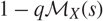 $1-q\mathcal{M}_{X}(s)$ determine 𝔪-poles of
 $\mathcal{M}_{R^{+}}$ for use in the higher-order expansions of Corollary 3.
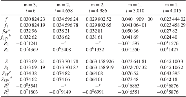
Various density and survival function approximations for the true density f (t) and survival S(t) in three settings: using a negative binomial (𝔪,  $\tfrac12$) weight distribution with 𝔪 = 3, 2, and 1 along with an extreme value claim distribution. For various approximations, the last accurate digit is boldface.
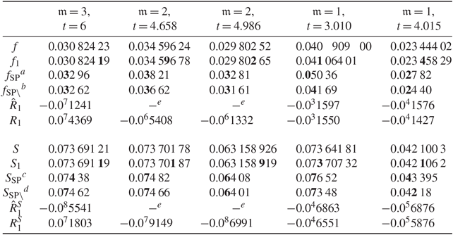
a,c Denotes a saddlepoint density or Lugannani and Rice (Reference Lugannani and Rice1980) survival approximation applied directly to  $\mathcal{P}\{\mathcal{M} _{X}(s)\}$ and retaining the point mass at t = 0.
b,d Denotes a saddlepoint density or Lugannani and Rice (Reference Lugannani and Rice1980) survival approximation applied to  $\mathcal{M}_{R^{+}}(s)$ and without the point mass and subsequently correcting by using the factor 1 − p(0).
e Path of steepest descent for computation lies in the directions θ = 0 and 180°.
The Laurent coefficients from the PGF of N are ρ −𝔪 = (− p/q)𝔪 and ρ −k = 0 for k = 1, …, 𝔪 − 1. Values in (27) are
 \beta_{-k}=\frac{\rho_{-\mathfrak{m}}}{(\mathfrak{m}-k)!}\frac{d^{\mathfrak{m} -k}}{ds^{\mathfrak{m}-k}}\Big(\frac{1}{\{\mathcal{N}(s)\}^{\mathfrak{m}} }\Big) _{s=b},\qquadk=1,\ldots,\mathfrak{m}-1.
Example 17. (Extreme value claims, right tail.) Suppose claims follow an extreme value distribution with support (− ∞, ∞) and MGF  $\mathcal{M}_{X}(s)=\Gamma(1-s)$. In Table 3 we show expansion approximations f 1 and S 1 for the density and survival function of R using negative binomial
 $(\mathfrak{m},\tfrac12)$ weight distributions, with 𝔪 = 3, 2, and 1. We used t = 6 in the 𝔪 = 3 case and chose values for t in the 𝔪 = 2 and 𝔪 = 1 cases which are designed to maintain a comparable percentile location both unconditionally, with t = 4.658 and 3.010, respectively, and conditionally (given X ≠ 0), with t = 4.986 and 4.015, respectively. The rationale for this is that the accuracy of such expansions can be expected to improve as t → ∞, so in order to determine accuracy as the pole order m changes, the percentile rank of t should stay fixed.
A comparison of f (t) with f 1(t) and S(t) with S 1(t) leads to the following observations. For m fixed, accuracy increases with t as expected. If the percentile rank of t is held fixed for R|R ≠ 0, so the accuracy comparison involves columns 2, 4, and 6, then accuracy decreases as the pole order decreases from 𝔪 = 3 to 1.
All 𝔪 terms in expansions (26) and (28) are needed in order to attain the high accuracy seen in the table. For density approximation, if only the leading term in (26) of order O(e−btt 𝔪−1) is used in the 𝔪 = 3 and 𝔪 = 2 cases, then the resulting approximate density values are not accurate. This leading term attains the values 0.02674, 0.0168, and 0.0150 respectively over columns 2–4. For the survival function, the leading term of order O(S G(𝔪,b)(t)) is not accurate either and attains the respective values 0.0215, 0.0417, and 0.0365.
First-order expansions are least accurate for 𝔪 = 1; however, saddlepoint error corrections also substantially improve accuracy in this case. When t = 3.010 (4.015) then f 1 + R̂ 1 = 0.040 904 (0.023 443) and each error correction adds one further digit of accuracy; also S 1 + $\hat{R}_{1}^{S}=0.073\,6\mathbf{3}9$ $(0.042\,0\mathbf{9}9)$ and error correction adds two (one) additional digits of accuracy.
Saddlepoint density approximations f SP(t) and f SP\(t) in Table 3 are based on the approximation (22) applied with and without the point mass p(0) included in the MGF used for the approximation. Thus, we approximate f (t) either directly from  $\mathcal{M}_{R}$ to get f SP(t), or indirectly from
 $\mathcal{M}_{R^{+}}$ to get f SP\(t), through f (t) = {1 − p(0)}fR+ (t) 1{t>0}. Likewise, S SP(t) and S SP\(t) use the Lugannani-Rice approximation (Butler (Reference Butler2007, Section 1.2.1)) to approximate S(t) either directly or else indirectly through S(t) = {1 − p(0)}SR+(t) 1{t>0}. Both approximations provide adequate accuracy for all these applications but do not achieve the extraordinary accuracy of f 1(t) and S 1(t). Approximations f SP\(t) and S SP\(t) have comparable accuracy to their counterparts f SP(t) and S SP(t) for m = 3 and 2 and show slightly greater accuracy with 𝔪 = 1. This is explained by the fact that p(0) increases as m decreases so more mass is placed at 0 and the methods that do not remove this point mass encounter greater difficulty and, hence, lose accuracy.
3.2.1. Inversion integration and the analytic continuation of $\mathcal{P}\{\mathcal{M}_{X}(s)\}$

The expansions of Theorems 1 and 2 do not apply directly to the density and survival of R, but rather indirectly by way of the absolutely continuous distribution for R + = R| R = 0 with MGF  $\mathcal{M}_{R^{+} }(s)=[\mathcal{P}\{\mathcal{M}_{X}(s)\}-p(0)]/\{1-p(0)\}$, density fR+ (t), and survival SR+ (t); thus, the relations fR(t) = {1 − p(0)}fR+(t) and SR(t) = {1 − p(0)}SR+ (t) for t > 0 lead to the expansions in Theorem 3 for the distribution of R. In fact, if the density inversion integral in (4) were used with MGF
 $\mathcal{P} \{\mathcal{M}_{X}(s)\}$, then it would not converge due to the leading term p(0) > 0 in its expansion. Using
 $\mathcal{P}\{\mathcal{M}_{X}(s)\}$ in the survival inversion integral (54) of Butler (Reference Butler2019a, Section 5.1.4) results in a conditionally convergent principal-value integral but not an absolutely convergent integral; thus, numerical inversion requires integration from ε − Ni to ε + Ni for quite large N. By comparison, both of these integrals are absolutely convergent using
 $\mathcal{M}_{R^{+}}(s)$ if
 $|\mathcal{M}_{X}(\varepsilon+\im y)|=O(|y|^{-1-\alpha})$ as y → ∞ for some α > 0. From a practical perspective, however, absolute convergence is typically not enough and α must be large if the numerical inversion is to be accurate using reasonable values of N.
For our example, the ‘exact’ computations for f (t) and S(t) in Table 3 were based on the numerical inversion of  $\mathcal{M}_{R^{+}}(s)$ to determine fR+ (t) and SR+ (t). The integration was in the convergence strip along the contour line {Re(s) = ŝ 0} determined by saddlepoint ŝ 0 ∈ (0, b) which solves
 $\rd\ln\,\{\mathcal{M}_{R^{+} }(s)\}/\sd s=t$. This leads to an inversion integral expression
 \begin{equation}f_{R^{+}}(t)\approx \re^{-\hat{s}_{0}t}\frac{1}{\pi}\int_{0}^{N}{\mathrm{Re}}\{\mathcal{M}_{R^{+}}(\hat{s}_{0}+\im y)\re^{-\im ty}\}\sd y\end{equation}
for sufficiently large N. Survival SR+ (t) is determined as in (34) by including the additional factor (ŝ 0 + iy)−1 in the argument of Re{·} in the integrand. We used N = 20 to obtain a 17 digit accuracy based on an inversion integrand which, from (33), has the order
 |\mathcal{M}_{R^{+}}(\hat{s}_{0}+\im y)|\sim\frac{p^{\mathfrak{m}}\mathfrak{m} q}{1-p^{\mathfrak{m}}}|\Gamma(1-\hat{s}_{0}-\im y)|=O(|y|^{1/2-\hat{s}_{0} }\re^{-\pi|y|/2}),\qquad |y|\rightarrow\infty,
with ŝ 0 ∈ (0, 0.55); see 5.11.9 of NIST DLMF (Reference Nist2014).
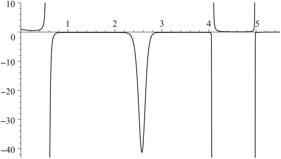
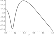
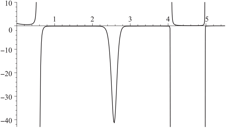
Plot of  $\mathcal{M}_{R^{+}}(s)\re^{-6s}$ versus s ∈ [0, 5.5] for the 𝔪=3 setting showing the real poles as well as the potential for saddlepoints at critical values in between the integers 1–5.
The analytic continuation of  $\mathcal{P}\{\mathcal{M} _{X}(s)\}$. The m-pole b = 0.5571 applies to all five examples in Table 3 since it is a pole for the factor {2 − Г(1 − s)}−𝔪, which appears in
 $\mathcal{P}\{\mathcal{M}_{X}(s)\}$ and
 $\mathcal{M}_{R^{+}}(s)$. The exact remainder terms R 1(t) and
 $R_{1}^{S}(t)$ in Table 3 were computed using numerical inversion of
 $\mathcal{M}_{R^{+}}(s)$ as in (34) but rather passing the vertical contour through ŝ 1, the closest real saddlepoint above b. In each of the five examples, Cauchy’s theorem, as reflected in the identities f (t) = f 1(t) + R 1(t) and
 $S(t)=S_{1}(t)+R_{1}^{S}(t)$, was confirmed to 17 significant digits through numerical computation of f (t), R 1(t), S(t), and S 1(t) using MAPLE®.
In the analytic continuation of  $\mathcal{M}_{R^{+}}(s)$ in which Re(s) > b, there are poles at b 2± = 2.581 ± 0.1723i, b 3 = 4.076, 4.978, 6.004, 6.999, … arising as zeros of 2 − Г(1 − s). For the 𝔪 = 3 example, Figure 1 shows a plot of
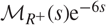 $\mathcal{M}_{R^{+}}(s)\re^{-6s}$ which captures these real poles as well as potential saddlepoints spaced in between the integers 1 − 5. Saddlepoints are located at 0.2687, 2.196, 2.546, 4.019, and 4.838. For all saddlepoints except 2.546, Figure 1 suggests that
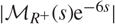 $|\mathcal{M}_{R^{+}}(s)\re^{-6s}|$ has a local minimum at each of these saddlepoints along the real line. This is indeed the case as
 $\mathcal{K}_{R^{+}}^{\prime\prime}>0$ at each of these saddlepoints so the steepest descent (ascent) directions are ±90° (0°, 180°) and the saddlepoint is ‘vertically oriented’. By contrast, the saddlepoint at 2.546 occurs at a local maximum for
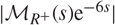 $|\mathcal{M}_{R^{+}}(s)\re^{-6s}|$ along the real line. This is confirmed by computing
 $\mathcal{K}_{R^{+}} ^{\prime\prime}(2.546)<0$ so its steepest descent (ascent) directions are θ = 0°, 180° (± 90°) and are horizontally oriented. Thus, the geometry at 2.546 shows a real saddlepoint roughly in between the complex conjugate pair of poles b 2± which have the bearings ±1.370 = ±78.5°.
The extraordinary accuracy of f 1(t) and S 1(t) in the examples of Table 3 is partly due to having the poles b 2± lying well above b = 0.5571, so the asymptotic order of error is O(e−Re(b 2+)t).
The computations for R 1(t) and  $R_{1}^{S}(t)$ integrate along the respective contours {Re(s) = ŝ 1} and
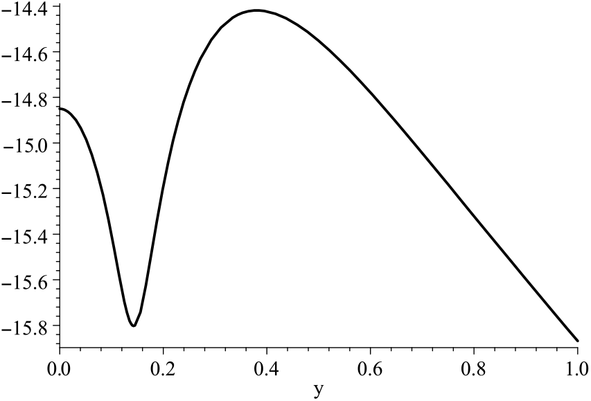
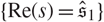 $\{{\mathrm{Re}}(s)=\mathfrak{\hat{s}}_{1}\}$. In Figure 2 we plot the modulus of the integrand along the former contour leaving saddlepoint ŝ 1 = 2.196. While the steepest descent curve is tangent at ŝ 1, it clearly deviates from this vertical line quite quickly since, for y > 0.14, the modulus increases along the vertical line due to the presence of the pole at 2.581 + 0.1723i.
In all the cases for which entries of R̂ 1(t) and  $\hat{R}_{1}^{S}(t)$ are given in Table 3, the next highest saddlepoint above b is vertically oriented and the saddlepoint approximation at this saddlepoint gives a reasonable assessment for the error magnitude in Cauchy’s theorem. In the 𝔪 = 2 case, these saddlepoints were horizontally oriented and this leads to inaccuracy when approximating R 1(t) and
 $R_{1}^{S}(t)$. For example, in the case t = 4.658, R̂ 1(t) = 0.03146i and
 $\hat{R} _{1}^{S}(t)=0.0^{3}149\im$ and the imaginary factor i results from the contour integral passing horizontally through the saddlepoints at ŝ 1 = 0.861 and
 $\mathfrak{\hat{s}}_{1}=0.851$, respectively, to the right of pole b. Apart from the obviously incorrect imaginary factors, their magnitudes are also quite far from the true values of R 1(t) and
 $R_{1}^{S}(t)$. Judging from this example and others, the accuracy of saddlepoint computations as error approximations are in doubt if the saddlepoints are horizontally oriented.
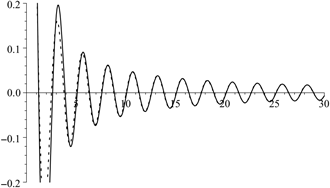
Plot of  ${\mathrm{Re}}\{\mathcal{K}_{R^{+}} (\hat{s}_{1}+\im y)-6(\hat{s}_{1}+\im y)\}$ versus y ∈ [0, 1] for the 𝔪 = 3 setting, where ŝ 1 = 2.196. The path of steepest descent is tangent at ŝ 1 (y = 0).
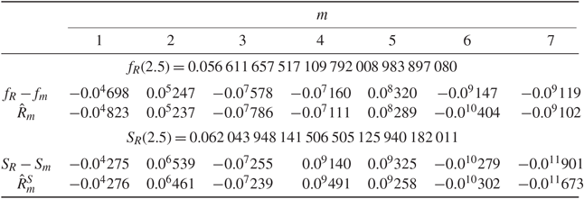
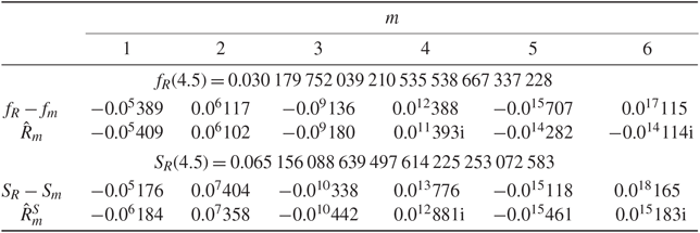
4. Sparre Andersen and Cramér–Lundberg models
Suppose claims for an insurance company arrive as a renewal process with interarrival times {Ti} that are i.i.d. and absolutely continuous with MGF  $\mathcal{M}_{T}$ convergent on {Re(s) > a} or {Re(s) ≤ a} with 0 < a ≤ ∞. Let the claim amounts {Xi} be positive, i.i.d., and absolutely continuous with MGF
 $\mathcal{M}_{X}$ convergent on {Re(s) < c} or {Re(s) ≤ c} with 0 < c ≤ ∞. Suppose that the company’s premiums increase revenue at the constant rate σ > 0 such that
 $\sigma>0$ so the random walk
 $\sum_{i=1}^{n}(X_{i}-\sigma T_{i} )=:\sum_{i=1}^{n}Y_{i}=:S_{n}$, which measures the company loss, has a negative drift. Under such circumstances, the maximum loss R = supn≥1 Sn is known to have a compound geometric distribution with MGF
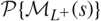 $\mathcal{P}\{\mathcal{M}_{L^{+}}(s)\}$ in which
 $\mathcal{P}(z)=\re^{-B} /\{1-(1-\re^{-B})z\}$ gives geometric (e−B) weights with
 $B=\sum _{n=1}^{\infty}\Pb(S_{n}>0)/n<\infty$. The MGF
 $\mathcal{M}_{L^{+}}(s)$ is that of the ascending ladder distribution of the random walk {Sn} and has been discussed extensively in Feller (Reference Feller1971, Chapter XII). Wiener–Hopf factorization is used to extract
 $\mathcal{M}_{L^{+}}$ from
 $\mathcal{M}_{Y}(s)=\mathcal{M} _{X}(s)\mathcal{M}_{T}(-\sigma s)$, the MGF of Y = X − σT. The convergence domain for
 $\mathcal{M}_{L^{+}}$ is {Re(s) < c} and, assuming that
 $1<\mathcal{M}_{Y}(c)\leq\infty$, the convergence domain for
 $\mathcal{M}_{L^{+}}$ is {Re(s) < b}, where b is the unique positive real root of
 $\mathcal{M}_{Y}(s)=1$ in (0, c). Feller (Reference Feller1971, Chapter XVIII, Sections 3–5) discusses Wiener–Hopf factorization and Butler (Reference Butler2017, Appendix B.4.2) summarises much that is relevant to our discussion. Density and survival function expansions for R, as in Theorem 3, can be derived, but the integrability conditions
 $\mathcal{AI}_{\rm p}^{\rm CD}$ and
 $\mathcal{UI}^{\rm CD}$ do not seem especially suitable in this context as they can be difficult to verify for
 $\mathcal{M} _{L^{+}}$. The density
 $f_{L^{+}}(t)$ and, hence, eb +tf L+ (t) are most often discontinuous at t = 0, so that transform
 $\mathcal{M}_{L^{+} }(b^{+}+\im y)$ is not absolutely integrable in y (Feller (Reference Feller1971, Chapter XV.3, Theorem 3)) and this refutes a simple sufficient condition for
 $\mathcal{AI}_{\rm p}^{\rm CD}$ and
 $\mathcal{UI}^{\rm CD}$. Furthermore,
 $\mathcal{BV}^{\rm CD}$ is difficult to verify since fL+ (t) is more often intractable. We instead develop the conclusions of Theorem 3 under some alternative conditions
 $\mathcal{AC}^{\rm SA}$ and
 $\mathcal{AI}_{\rm p}^{\rm SA}$ given below, which are more practically useful and suited for distributions with support on (0, ∞). A proof is given in Section 5.4.1 of Butler (Reference Butler2019a).
- $\mathcal{AC}^{\rm SA}$. For some ε 1 ∈ (0, c – b), $\int_{0^{-}}^{\infty}\re^{(b+\varepsilon_{1})t}\sd f_{L^{+}} (t)$ is absolutely convergent.
- $\mathcal{AI}_{\rm p}^{\rm SA}$. For some ε 1 ∈ (0, c – b), $|\mathcal{M}_{L^{+}}(b+\varepsilon_{1}+\im y)|^{p} $ is integrable in y for some p > 1.




Theorem 4. (Sparre Andersen model.) Let  $\mathcal{M}_{T}$,
 $\mathcal{M}_{X}$, and
 $\mathcal{P}$ be as described above so that b ∈ (0, c) is a simple pole of
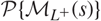 $\mathcal{P}\{\mathcal{M}_{L^{+}}(s)\}$.
Under condition  $\mathcal{AC}^{SA}$,
 \begin{equation}f_{R}(t)=\re^{-bt}(\!-\beta_{-1})+o(\re^{-(\beta+\varepsilon)t}),\qquadt\rightarrow\infty,\end{equation}
for sufficiently small ε ∈ (0, ε 1), where  $\beta_{-1}=\operatorname*{Res}[\mathcal{P} \{\mathcal{M}_{L^{+}}(s)\},b]$.
If either of the conditions  $\mathcal{AC}^{SA}$ or
 $\mathcal{AI}_{p}^{SA}$ holds, then
 \begin{equation}S_{R}(t)=\frac{\re^{-bt}(\!-\beta_{-1})}{b}+o(\re^{-(b+\varepsilon)t}),\qquad t\rightarrow \infty,\end{equation}
for sufficiently small ε ∈ (0, ε 1).
The expansion of SR(t) in (36) is the classical result given in Theorem 3.1, Case (i) of Embrechts and Veraverbeke (Reference Embrechts and Veraverbeke1982). Density expansion (35), which implies (36), was first shown to hold in Butler (Reference Butler2017, Section 5.2) under more restrictive conditions on the MGF and density of X. By comparison, the assumptions  $\mathcal{AC}^{\rm SA}$ and
 $\mathcal{AI}_{\rm p}^{\rm SA}$ place conditions on
 $\mathcal{M}_{L^{+}}$ and f L + which tend to be weaker and more inclusive, but perhaps more difficult to check in settings where f L + is not tractable.
Conditions  $\mathcal{AC}^{\rm SA}$ and
 $\mathcal{AI}_{\rm p}^{\rm SA}$, however, are ideally suited for the Cramér–Lundberg setting in which density f L + and MGF
 $\mathcal{M}_{L^{+}}$ take on explicit forms. In this context it is easily shown that conditions
 $\mathcal{AC}^{\rm SA} $ and
 $\mathcal{AI}_{\rm p}^{\rm SA}$ and Theorem 4 hold without further qualification; see Section 5.4.2 of Butler (Reference Butler2019a). In the Cramér–Lundberg setting the renewal process for claim arrivals is a Poisson (λ) process so that interarrival times {Ti} for claims are i.i.d. Exponential (λ). If
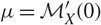 $\mu=\mathcal{M}_{X}^{\prime}(0)$ then B = − ln(1 − ρ), where ρ = λμ/σ < 1 ensures that the random walk
 $\sum_{i=1}^{n}Y_{i}$ has a negative drift. The ascending ladder distribution has density f L + (t) = SX(t)/μ, which is the excess life density with MGF
 $\mathcal{M}_{L^{+}}(s)=\{1-\mathcal{M}_{X}(s)\}/(-\mu s)$. See Section 5.4.2 of Butler (Reference Butler2019a) for more details.
Corollary 4. (Cramér–Lundberg model.) Suppose that  $\mathcal{M}_{X}$ is as described above,
 $\mathcal{M}_{T}(s)=(1-s/\lambda)^{-1}$, and
 $\mathcal{P} (z)=(1-\rho)/(1-\rho z)$. Let b be the smallest positive root of
 $\rho\mathcal{M}_{L^{+}}(s)=1$ in (0, c). Then conditions
 $\mathcal{AC}^{SA}$ and
 $\mathcal{AI}_{p}^{SA}$ hold without further conditions, so that
 \begin{align}f_{R}(t) = (1-\rho)\re^{-bt}\frac{b}{\lambda \mathcal{M}_{X}^{\prime}(b)/\sigma-1} +o(\re^{-(b+\varepsilon)t}),\qquad t\rightarrow\infty,\end{align}
 \begin{align}S_{R}(t) = (1-\rho)\re^{-bt}\frac{1}{\lambda \mathcal{M}_{X}^{\prime}(b) \sigma-1}+o(\re^{-(b+\varepsilon)t}),\qquad t\rightarrow\infty,\end{align}
for sufficiently small ε ∈ (0, c − b).
The survival expansion (38) is the classical Cramér–Lundberg approximation for ruin probability as given in Asmussen (Reference Asmussen2000, III.5, Theorem 5.3). Expansion (37), which implies (38), was first derived in Butler (Reference Butler2017, Section 5.1) under restrictive conditions on the MGF and density of X.
The expansions for fR and SR in both Theorem 4 and Corollary 4 hold to higher asymptotic order (for larger values of ε > 0) if MGF
 \begin{equation}\mathcal{M}_{R^{+}}(s)=\frac{(1-\rho)\mathcal{M}_{L^{+}}(s)}{1-\rho \mathcal{M}_{L^{+}}(s)},\qquad{\mathrm{Re}}(s)<b, \end{equation}
can be analytically extended to Re(s) < b + ε 0}\{b} for some ε 0 > 0. Corollary 9 of Butler (Reference Butler2019a, Section 5.4.3) gives the precise conditions.
4.1. Higher-order expansions for the Cramér–Lundberg model
Increasingly accurate approximations can be obtained by adding in additional residue terms when  $\mathcal{M}_{R^{+}}$ in (39) admits an increasing sequence of simple real poles or complex conjugate pairs. The next result is new and follows from Corollary 3 as shown in Section 5.4.4 of Butler (Reference Butler2019a).
Corollary 5. (Cramér–Lundberg model.) Assume that the conditions of Corollary 4 hold. Suppose, furthermore, that  $\mathcal{M}_{R^{+}}$ can be analytically continued as in
 $\mathcal{AC}_{m}^{CD}$ and that
 $\mathcal{M}_{X}$ satisfies
 $\mathcal{X}_{m}^{CL}$.
- $\mathcal{X}_{\rm m}^{\rm CL}$. If bm > c, then εm ∈ (0, ε 0) exists such that $\max_{c\leq x\leq b_{m}^{+}}|\mathcal{M}_{X}(x+iN)|\rightarrow0$ as N → ∞, where $b_{m}^{+}=b_{m}+\varepsilon_{m}$ and ε 0 is specified in condition $\mathcal{AC}_{m}^{CD}$.


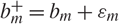

For real-valued poles, then
 \begin{align}f_{R}(t) = f_{m}(t)+R_{m}(t)\coloneqq(1-\rho)\sum_{k=1}^{m}\re^{-b_{k}t}\frac{b_{k}}{\lambda\mathcal{M}_{X}^{\prime}(b_{k})/\sigma-1}+o(\re^{-b_{m}^{+}t}),\end{align}
 \begin{align}S_{R}(t) = S_{m}(t)+R_{m}^{S}(t)\coloneqq(1-\rho)\sum_{k=1}^{m}\re^{-b_{k}t}\frac {1}{\lambda\mathcal{M}_{X}^{\prime}(b_{k})/\sigma-1}+o(\re^{-b_{m}^{+}t}),\end{align}
as t → ∞. Here,
 \begin{equation}R_{m}(t)=\frac{1-\rho}{2\pi}\re^{-b_{m}^{+}t}\int_{-\infty}^{\infty} \mathcal{M}_{R^{+}}(b_{m}^{+}+\im y)\re^{-\im ty}\sd y,\end{equation}
and  $R_{m}^{S}(t)$ is expression (42) with the additional integrand term
 $(b_{m}^{+}+\im y)^{-1}$. The same expansions hold with complex conjugate pairs of poles when summed over all pairs of poles.
4.2. Heavy-traffic diffusion approximations
Siegmund (Reference Siegmund1979) and Blanchet and Glynn (Reference Blanchet and Glynn2006) provided diffusion or heavy-traffic approximations for the distribution of R in the Sparre Andersen model which are directly related to the expansions above. In particular, the complete asymptotic expansion of Blanchet and Glynn (Reference Blanchet and Glynn2006, Equation 5) is exactly the survival expansion (36) in Theorem 4, and the corrected diffusion approximation of Siegmund (Reference Siegmund1979, Equation 28) is a lower-order approximation to this expansion as discussed further below. The importance of these papers is that they address the computation of the residue coefficient  $\beta_{-1}=\operatorname*{Res} [\mathcal{P}\{\mathcal{M}_{L^{+}}(s)\},b],$, a task made quite difficult due to its dependence on
 $\mathcal{M}_{L^{+}}$. These papers are less relevant in the Cramér–Lundberg setting since explicit values for this residue are available and so the complete expansion of Blanchet and Glynn (Reference Blanchet and Glynn2006, Equation 5) is given in (38) of Corollary 4 with even higher-order terms in (41) of Corollary 5.
Heavy traffic is related to properties of the convex function  $\mathcal{K} _{Y}(s)=\ln\mathcal{M}_{Y}(s)$ for the random step size Y. From Siegmund (Reference Siegmund1979), the adjustment coefficient Δ = b − 0 since 0 and b are the unique zeros for
 $\mathcal{K}_{Y}(s)$. Heavy traffic occurs when the negative drift of the random walk
 $\mathcal{K}_{Y}^{\prime}(0)\uparrow0$ and Δ = b ↓ 0. In terms of convex
 $\mathcal{K}_{Y}$, this means that the value and location of its minimum approach 0. The asymptotic regime for heavy traffic has t → ∞, b ↓ 0, and bt → ξ > 0; see Siegmund (Reference Siegmund1979). The expansion in (36) holds under asymptotic regime t → ∞ so it also holds under the more restrictive heavy-traffic regime. Hence, equating the asymptotic expansion in (36) with that in Blanchet and Glynn (Reference Blanchet and Glynn2006, Equation 5) shows their leading terms must be the same within the heavy-traffic asymptotic regime.
This discussion suggests that improvement over the expansions in both Siegmund (Reference Siegmund1979) and Blanchet and Glynn (Reference Blanchet and Glynn2006, Equation 5) is possible in the Sparre Andersen setting by using higher-order expansions comparable to those in Corollary 5. The impediment to this, however, is in determining the additional residues for poles of  $\mathcal{P}\{\mathcal{M}_{L^{+}}(s)\}$ further into its analytic continuation.
4.3. Applications and Cramér–Lundberg examples
Wiener–Hopf factorization in the Sparre Andersen model leads to an explicit rational form for  $\mathcal{M}_{L^{+}}$ when
 $\mathcal{M}_{Y}(s)=\mathcal{M} _{X}(s)\mathcal{M}_{T}(-\sigma s)$ is a rational function and B < ∞. Factorization of
 $1-\mathcal{M}_{Y}(s)$ into monomials in its numerator and denominator fully identifies those monomials belonging to the rational factor that determines
 $\mathcal{M}_{L^{+}}(s)$, so that
 $\mathcal{M}_{L^{+}}$ is rational; see Butler (Reference Butler2017, Section B.4.2). Since
 $\mathcal{P}$ is rational, then
 $\mathcal{P}\{\mathcal{M}_{L^{+}}(s)\}$ is rational and its partial fraction expansion leads to exact computation of the density and survival function of R +.
By contrast, when  $\mathcal{M}_{Y}$ is not rational, then extraction of
 $\mathcal{M}_{L^{+}}(s)$ is quite difficult except in the Cramér–Lundberg setting where
 $\mathcal{M}_{L^{+}}$ is the excess life MGF constructed from
 $\mathcal{M}_{X}$. Tijms (Reference Tijms2003, Section 9.2.2) considered two Cramér–Lundberg examples which use hyperexponential and Erlang claim distributions. In both instances, however,
 $\mathcal{M}_{X}$ is rational which leads to rational expressions for
 $\mathcal{M}_{L^{+}}(s)=\{1-\mathcal{M}_{X}(s)\}/(-\mu s)$ and an exact analysis is possible through partial fraction expansion. We avoid these simpler situations by presenting two examples in which
 $\mathcal{M} _{L^{+}}$ is not rational. In the first example,
 $\mathcal{M}_{X}$ is an entire function while in the second example,
 $\mathcal{M}_{X}$ admits a sequence of increasing poles.
Example 18. (Cramér–Lundberg, Raleigh (1) claims.) Assume that claims follow a Raleigh (1) distribution with mean 1. Take λ = 1 and σ = 2 so that ρ = 1/2. We wish to determine f (2.5) and S(2.5) using higher-order expansions. In Figure 3 we show a sequence of simple poles (◊) for  $\mathcal{M}_{R^{+}}(x+\im y)$ which occur as zeros for denominator
 $1-\rho\mathcal{M}_{L^{+}}(s)$ with b = 0.913 (◊) as the real pole at the boundary of convergence. Higher-order poles lie approximately on the 45° line with x ≈ y. Interspersed in between the poles are saddlepoints (°) for
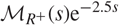 $\mathcal{M}_{R^{+}}(s)\re^{-2.5s}$. The lines through the saddlepoints indicate the directions of steepest descent. Not shown are the matching complex conjugate poles and saddlepoints located below the real axis. Real saddlepoint ŝ 0 = 0.4753(°) lies inside the convergence domain.
In Table 4 we show the accuracy for asymptotic expansions in (40) and (41) of orders m = 1 to m = 7 for the values fR(2.5) and SR(2.5). First-order expansion f 1(2.5) = 0.056 68 attains 4 (3 significant) digit accuracy and this exceeds the accuracy of saddlepoint approximation f SP\ (2.5) = 0.060 46. First-order expansion S 1(2.5) = 0.062 071 4 attains similar accuracy and exceeds that of saddlepoint approximation S SP\ (2.5) = 0.062 17.
A plot showing the alternating pattern of poles (◊) and saddlepoints (°) for 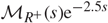 $\mathcal{M}_{R^{+}}(s)\re^{-2.5s}$ for s = x + iy ∈ ℂ with x, y ≥ 0. Lines through saddlepoints indicate the directions of steepest descent.
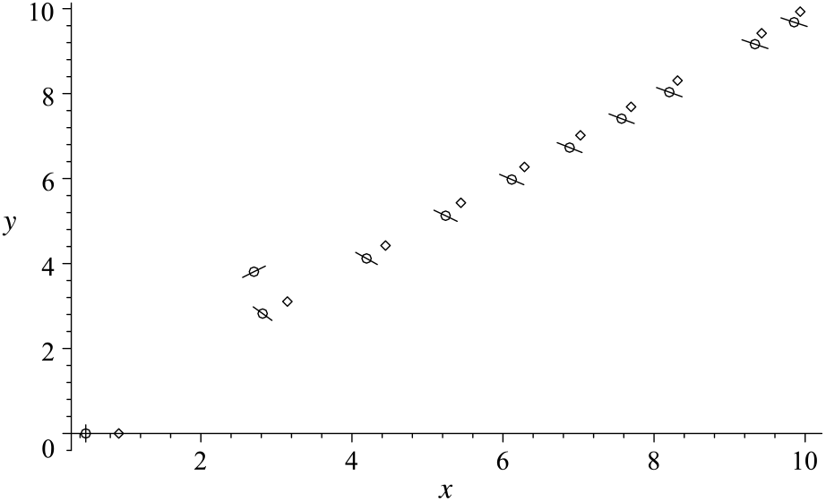
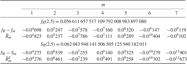
Exact values for fR and SR are displayed to a 30 decimal point accuracy and were computed using numerical integration which roughly follows the path of steepest descent from ŝ 0 as described in Section 4.4 below.
There are some subtleties concerning how the saddlepoint computations were made. The saddlepoint density value f SP\ (2.5) = 0.060 46 results if (22) is used only with ŝ 0 = 0.4753. However, upon viewing the pattern of saddlepoints and poles in Figure 3, additional saddlepoint terms are needed to approximate f (2.5) when based on the method of steepest descents. The contour for this path must be deformed to pass through the saddlepoint ŝ 0 but also the saddlepoints ŝ 1± = 2.703 ± 3.807i with steepest descent directions ±0.723 ≈ ±41.4°. The sum of all three contributions is 0.060 44 and about the same value. Likewise, in the computation of R̂ 1, saddlepoint computation requires summing four contributions over ŝ 1± and ŝ 2± = 2.817 ± 2.821i with the latter having steepest descent directions ±2.23 ≈ ±128.0°. This yields the value for R̂ 1 in Table 4. The value S SP \(2.5) = 0.062 17 was computed using the Lugannani–Rice approximation, which accommodates for the pole at s = 0 using the Bleistein (Reference Bleistein1966) method, but which is not based upon following the path of steepest descent. Saddlepoint approximation using (23) and summing over saddlepoints 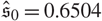 $\mathfrak{\hat{s}}_{0}=0.6504$ and
 $\mathfrak{\hat{s}}_{1\pm}=2.679\pm3.794\im$ leads to 0.058 17 which, as expected, is less accurate due to not accommodating the pole at s = 0.
(Cramér–Lundberg, truncated extreme value claims). Errors of various residue approximations for density and survival function values fR(4.5) and SR(4.5) using a truncated extreme value claim distribution. For a description of other entries, see Table 2.
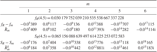
Example 19. (Cramér–Lundberg, truncated extreme value claims.) Assume that the claim distribution has the density (1 − e−1) exp (− t − e−t) 1{t>0} with mean μ = 1.260. Its MGF is derived in Section 5.4.8 of Butler (Reference Butler2019a) as
 \begin{equation}\mathcal{M}_{X}(s)=\frac{1}{1-\re^{-1}}\frac{1}{1-s}\,_{1}F_{1}(1-s;2-s;-1),\end{equation}
where 1F 1 denotes the confluent hypergeometric function. Expression (43) admits simple poles at s 𢘈 {1, 2, . . .} at which  $\mathcal{M}_{R^{+}}(s)$ is analytic. Interspersed between these poles are simple zeros for the denominator of
 $\mathcal{M}_{R^{+}}(s)$ which occur at
 \begin{align*}b=b_{1}=0.4632<b_{2}=2.226<2.896<4.023<4.995<6.001=b_{6}.\end{align*}
We choose λ = 1/μ and σ = 2 so that  $\rho=\tfrac12$. In between the poles, there are real saddlepoints for
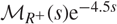 $\mathcal{M}_{R^{+}}(s)\re^{-4.5s}$ which are used to approximate error terms for fR(4.5). They occur at
 \hat{s}_{1}=2.049<2.735<3.906<4.312(-)<5.958<6.055(-)=\hat{s}_{6},
where the negative sign (no sign) indicates a saddlepoint that is oriented horizontally (vertically) so the path of steepest descent is in directions 0, π (± π/2). Slightly different saddlepoints apply when dealing with the survival inversion.
In Table 5 we show that increasingly accurate approximations can be obtained by adding in additional residue terms from these simple poles. The leading residue terms f 1(4.5) = 0.030 175 8 and S 1(4.5) = 0.065 154 3 achieve a 5 and 4 decimal point accuracy, and this exceeds that of the saddlepoint approximations f SP\ (4.5) = 0.032 54 and S SP\(4.5) = 0.065 21, which achieve a 2 and 4 decimal point accuracy. Each additional residue term contributes 2 or 3 more accurate digits in the expansions. The saddlepoint computation of errors R̂m(4.5) and  $\hat{R}_{m}^{S}(4.5)$ provides a reliable guide for expansion accuracy by capturing the correct order for error except, as previously seen, when horizontally oriented saddlepoints are involved.
Exact computations of fR(4.5) and SR(4.5) were computed by roughly following the path of steepest descent as described below.
(Raleigh claim distribution). A plot of  ${\mathrm{Re}} \{\mathcal{M}_{R^{+}}(\hat{s}_{0}+\im y)\re^{-\im ty}\}$ versus y (solid line) and its asymptotic expression μ −1(1 − ρ)y −1 sin (ty) versus y (dashed line) shows that the former plot resembles a slowly dampened sine function. Here, t = 2.5, μ = 1, and
 $\rho=\tfrac12$.
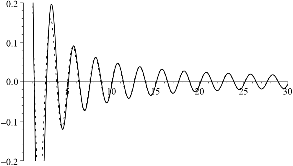
4.4. Steepest descent inversion required
In both examples of Section 4.3, numerical confirmation for the accuracy of various approximations for fR(t) and SR(t) required choosing inversion contours that are more specific to the examples than those in (34). In fact, for all Cramér–Lundberg examples, the integrand for the inversion in (34) is of order O{y −1 sin(ty)} as y → ∞ and not absolutely integrable. A proof is given in Section 5.4.5 of Butler (Reference Butler2019a).
Theorem 5. (Cramér–Lundberg inversion contour.) Let the inversion integral (34) for fR+ (t) use an arbitrary contour {Re(s) = x} for x ∈ [0, b). Then, the integrand in (34) for the resulting inversion integral which computes fR+ (t) has the asymptotic expansion
 \begin{equation}\re^{-xt}\frac{1}{\pi}{\mathrm{Re}}\{\mathcal{M}_{R^{+}}(x+\im y)\re^{-\im ty} \}\sim\frac{(1-\rho)\re^{-xt}}{\pi\mu}\frac{\sin(ty)}{y},\qquad y\rightarrow \infty.\end{equation}
Thus, the left-hand side of (44) is conditionally integrable in y but not absolutely integrable. The integrand for inversion of SR+ (t) if x ≠ 0 has the expansion
 \begin{equation}\re^{-xt}\frac{1}{\pi}{\mathrm{Re}}\Big\{ \frac{\mathcal{M}_{R^{+}}(x+\im y)\re^{-\im ty}}{x+\im y}\Big\} \sim\frac{(1-\rho)\re^{-xt}}{\pi\mu}\,\frac {\cos(ty)}{y^{2}},\qquad y\rightarrow\infty,\end{equation}
so the left-hand side of (45) is absolutely integrable but still converges very slowly.
In Figure 4 we show how quickly the inversion integrand for the density conforms to its oscillatory asymptotic expansion in (44) when x = ŝ 0. Such slowly dampened oscillations are a major impediment to accurate density and survival function inversion. To avoid such difficulties in our numerical computations, we deform the inversion contour so it becomes a contour ray which ultimately approximates the path of steepest descent in direction θ ∈ [0, π/2]. Instead of integrating from ŝ 0 − i∞ to ŝ 0 + i∞ as in (34), we choose ray angle θ above the real axis and ray angle −θ below the real axis. Thus, our deformation of the integration is along three lines: from ŝ 0 − iπ + e−iθ∞ to ŝ 0 − iπ to ŝ 0 + iπ to ŝ 0 + iπ + eiθ∞. As shown in Section 5.4.6 of Butler (Reference Butler2019a), this provides the following inversion expression.
Theorem 6. (Cramér–Lundberg deformed contour.) Let absolutely continuous variable R + have density fR+ (t) on (− ∞, ∞) which is locally of bounded variation at t. Suppose that its MGF  $\mathcal{M}_{R^{+}}(s)$ converges in the right half-plane on {0 ≤ Re(s) < b} for b > 0. Furthermore, assume that
 \begin{equation}\max_{\theta\leq\phi\leq\pi/2}|\mathcal{M}_{R^{+}}(\hat{s}_{0}+\im\pi+N\re^{\im\phi })|\rightarrow0, \qquad N\rightarrow\infty,\nonumber\end{equation}
and also assume that  $\mathcal{M}_{R^{+}}$ is analytic in the sector {ŝ 0 + iπ + reiϕ : r ≥ 0, ϕ ∈ [θ, π/2]}. Then, the inversion integral (4) for fR+ (t) which passes through the saddlepoint ŝ 0 may be deformed so that
 \begin{align}f_{R^{+}}(t) & = \re^{-\hat{s}_{0}t}\frac{1}{\pi}\int_{0}^{\pi}{\mathrm{Re}}\{\mathcal{M}_{R^{+}}(\hat{s}_{0}+\im y)\re^{-\im ty}\}\sd y\label{invertray}\end{align}
 \begin{align}&\jump +\re^{-\hat{s}_{0}t}\frac{1}{\pi}\int_{0}^{\infty}\operatorname{Im} [\mathcal{M}_{R^{+}}(\hat{s}_{0}+\im\pi+r\re^{\im\theta})\exp\{ \im(\theta -t\pi)-tr\re^{\im\theta}\} ] \sd r. \label{invertray2}\end{align}
The inversion for SR + (t) is the same as in (46) and (47) but includes the additional integrand factors (ŝ 0 + iy)−1 and (ŝ 0 + iπ + reiθ)−1 inside the curly and square braces of (46) and (47), respectively.
Contour deformation, as in Theorem 6, leads to extraordinary gains in computational efficiency over (34) for numerical inversion. This is demonstrated in Example 20, which provides a setting in which the ultimate steepest descent direction is θ ≈ 50.6°, and also in Example 21 where the ultimate direction is θ = 0.
Example 20. (Raleigh (1) claims.) Exact values for fR and SR in Table 4 are given to a 30 decimal point accuracy and were computed using (46) and (47) and following a ray that approximates the path of steepest descent. The improper integral in (47) was truncated at N = 60. This path starts at saddlepoint ŝ 0 = 0.4753 goes to ŝ 0 + iπ, and then follows the ray θ = 9π/32 ≈ 50.6° which lies slightly above the 45° ray on which we find the sequence of poles for  $\mathcal{M}_{R^{+}}$. These ‘exactly’ computed values were confirmed to agree (to 30 digits) with computed values for f 1 + R 1 and
 $S_{1} +R_{1}^{C}$, where R 1 and
 $R_{1}^{C}$ were computed as in (46) and (47) but with ŝ 0 replaced by 3 > b and using a slightly different direction θ = 10π/32 ≈ 56.2°.
By comparison, integration along the vertical contours in (34) with N = 500 was quite far from exact with fR(2.5) ≈ 0.056 593 and SR(2.5) ≈ 0.062 043 98. The density error is 0.0319 and less accurate than first-order approximation f 1(2.5) and the survival error is 0.0730 and comparable to S 3(2.5). The problem with accuracy is due to the slowly dampened and oscillatory nature of the integrand as seen in Figure 4 and highlighted in Theorem 5.
Example 21. (Truncated extreme value claims.) Exact computations of f (4.5) and S(4.5) used the inversion contour in (46) and (47) which passes through saddlepoint ŝ 0 = 0.4632, ŝ 0 + πi and follows a horizontal ray with θ = 0 and truncated with N = 60. Justification for using Theorem 6 is given in Section 5.4.8 of Butler (Reference Butler2019a). These computations were confirmed to a 30 digit accuracy using Cauchy’s theorem and passing the inversion also through saddlepoint ŝ 5 and using θ = π/32.
To determine what sort of accuracy can be achieved numerically when the contour of integration stays within the convergence region as in (34), we used integration on vertical contours with N = 500 and 502. Since the integrand is a slowly dampened sine wave, the numerical integration fluctuates with increasing N. A separation of 2 for N = 500 and 502 satisfies sin (4.5N) ≈ − sin{4.5(N + 2)} and should lead to two numerical results which have errors of opposite signs. This is what happened as we obtained f (4.5) ≈ 0.030 171 8 and 0.030 189 2 with errors 0.0579 and −0.0595, and S(4.5) ≈ 0.065 156 10 and 0.065 156 085 with errors of −0.0711 and 0.0837. Even with the use of such a massive amount of numerical integration within the convergence domain, we are only able to achieve roughly the accuracy of the first- and second-order expansions f 1 and S 2. Of course, the convergence acceleration methods of Abate and Whitt (Reference Abate and Whitt1992) and Strawderman (Reference Strawderman2004) can improve upon these results.
The problem with conventional inversion algorithms is their insistence on using vertical contours that stay in the convergence domain, which ensures that convergence is slow, rather than attempting to follow the path of steepest descent which is ultimately in some direction θ ∈ [0, π/2 − ε) and which takes the contour outside the convergence domain. If we deform the contour to crudely follow this path, as given in the integration formula of Theorem 6, then Example 21 shows that numerical integration in MAPLE® achieves a 30 digit accuracy using a contour that is  $12\%=100(\frac{60}{500})\%$ of the length used in following the vertical contours. Thus, our integration after deformation far outperforms the truncated integration along the vertical contour and is, furthermore, more stable and faster per unit of contour length. There seems to be no sensible reason for applying sophisticated convergence acceleration methods to slowly converging integrals in the convergence domain in the first place when much faster convergence can be achieved by deforming the contour to pass into the analytic continuation and to roughly follow the direction of steepest descent.
From a practical point of view, however, numerical integration is not even needed in this example since the first three residue terms suffice as a substitute for exact computation. We know this without making exact computations since the suggested saddlepoint approximations in the analytic continuation accurately provide the correct orders for these errors.
Acknowledgements
The author is grateful to a referee who drew attention to heavy-traffic/diffusion approximations and made suggestions to improve the presentation.