1. Introduction
This work is on fluid flow at high Reynolds number over a partly flexible surface. We are concerned especially with a flexible in-wall blip (a compliant patch forming a bump or a dip of finite length) which is tiny in the sense that its representative length scales along and normal to the otherwise fixed solid wall are very small compared with those of a boundary layer that is flowing over the wall. In fact the blip of theoretical concern here is so short and buried so low inside the boundary layer that only the near-wall part of the oncoming shear flow affects the local motion over the blip. Similar concern applies if several blips are present.
The applications motivating the work originally are in external flows in aerodynamics, sailing and past ice sheets. Carpenter & Garrad (Reference Carpenter and Garrad1985), Carpenter & Sen (Reference Carpenter and Sen1990), Gajjar & Sibanda (Reference Gajjar and Sibanda1996) and Gad-el-Hak (Reference Gad-el-Hak2000) primarily address perturbations for a compliant surface on an airfoil and find modes of instability stemming from those associated with a fixed surface. Fitt & Pope (Reference Fitt and Pope2001) and Alben & Shelley (Reference Alben and Shelley2008) discuss sail and flag flutter on inviscid grounds largely while Forbes (Reference Forbes1988) and Squire (Reference Squire1996) consider and compute surface waves and travelling loads on a model of an elastic plate. A common aim in aerodynamics and sailing for example is to promote drag reduction in which the near-surface flow is tripped beneficially causing transition to turbulence, as reviewed by Gad-el-Hak (Reference Gad-el-Hak2000) and Schlichting & Gersten (Reference Schlichting and Gersten2004). In many racing events (P. Bond, Private communication, 2010) engineering methods to reduce drag play an increasing part for rigid and flexible winged gliders, yachts, sails and hulls; the methods range from introducing surface-mounted trips (fixed bumps) or wall suction to special coatings or compliant surfaces intended to affect the boundary layer (Gad-el-Hak Reference Gad-el-Hak2000). The beneficial placing of a fixed trip depends sensitively however on the imposed pressure gradients and the local velocity profiles within the boundary layer. We are interested here in whether a so-called tuneable trip effect using a flexible blip instead may help produce total drag reduction, given that strong winds alter the oncoming flow and in particular alter the incident wall shear stress (WSS) significantly.
Previous relevant work tends to centre on periodic assumptions in the theoretical fluid/surface interaction, as in the pioneering studies of Benjamin (Reference Benjamin1960), Carpenter & Garrad (Reference Carpenter and Garrad1985) and Gajjar & Sibanda (Reference Gajjar and Sibanda1996), or on relatively large streamwise length scales that exceed the boundary-layer thickness to induce Tollmien–Schlichting instabilities (Smith Reference Smith1979; Lagrée Reference Lagrée2000), or both. Our interest is more in a tiny finite-length blip or several blips with fixed surface upstream and downstream, implying that periodicity is absent and the streamwise length scales are relatively small.
Applications also exist to internal flow such as that within a channel or pipe. See Hall & Smith (Reference Hall and Smith1982) and Green, Ovenden & Smith (Reference Green, Ovenden and Smith2009) on flexible-wall analysis and the very interesting string of studies by Pedley (Reference Pedley, Batchelor, Moffatt and Worster2000), Guneratne & Pedley (Reference Guneratne and Pedley2006), Kudenatti, Bujurke & Pedley (Reference Kudenatti, Bujurke and Pedley2012) and Pihler-Puzović & Pedley (Reference Pihler-Puzović and Pedley2013), on collapsible channel flows. The lateral pressure difference across the flexible blip surface is assumed to be directly related to the blip shape as in the external-flow references above. Here again the studies to date have tended to focus on length scales and corresponding time scales substantially larger than those of current concern.
Section 2 considers the incompressible viscous laminar properties due to the blip shape and the latter’s response to the fluid flow to yield two-way interaction in a planar setting, the typical blip length
 $l^{\ast }$
being much less than the typical development length
 $L^{\ast }$
of the boundary layer. Slowly evolving features are examined during a first stage to allow for significant changes in the parameters including the incident WSS. Linear and nonlinear interactive solutions for a single blip are investigated in §§ 3 and 4 which confirm the occurrence of intensifications, i.e. unduly large effects found for certain parameter values or eigenvalues. Special interest arises in forcing at low amplitudes because the intensifications and weakly nonlinear interactions appear to be unusual and lead on to rapidly evolving features as a second stage. Section 5 finds linear and nonlinear intensifications in the presence of many blips. These magnified effects for one or more tiny flexible blips are discussed further in § 6 along with potential repercussions.
2. Short blips
The typical tiny flexible blip is mounted on a solid surface such as an airfoil or bluff-body surface but the blip is so localised that the solid part of the surface may be considered as quasi-flat for most of our purposes. Concerning (first) the fluid dynamics, far from the surface the fluid is moving with a given constant velocity parallel to that flat part of the surface. The working below for two-dimensional flows incorporating short blips is expressed conveniently in terms of non-dimensional flow velocities
 $(u,v)$
, corresponding Cartesian coordinates
 $(x,y)$
, time
 $t$
and pressure
 $p$
, such that the dimensional versions are
 $U^{\ast }(u,v),L^{\ast }(x,y),L^{\ast }t/U^{\ast }$
and
 ${\it\rho}^{\ast }U^{\ast ^{2}}p$
, respectively. Here
 $U^{\ast }$
is the representative fluid velocity, taken to be the free-stream value above for definiteness, while
 $L^{\ast }$
is the typical length factor introduced in § 1,
 ${\it\rho}^{\ast }$
is the uniform density of the incompressible fluid and the temporal factor
 $L^{\ast }/U^{\ast }$
taken is the typical transport time. The continuity and Navier–Stokes equations of momentum balance are then
 $$\begin{eqnarray}\displaystyle & \mathbf{div}\,\boldsymbol{u}=0, & \displaystyle\end{eqnarray}$$
 $$\begin{eqnarray}\displaystyle & \boldsymbol{u}_{t}+(\boldsymbol{u}\boldsymbol{\cdot }\boldsymbol{{\rm\nabla}})\boldsymbol{u}=-\boldsymbol{{\rm\nabla}}\,p+\mathit{Re}^{-1}{\rm\nabla}^{2}\,\boldsymbol{u}, & \displaystyle\end{eqnarray}$$
 $\boldsymbol{u}=(u,v)$
, pressure
 $p$
and coordinates
 $x,y$
are generally of order unity except near the flat part of the solid surface which is located along the axis
 $y=0$
. In particular
 $\boldsymbol{u}$
is given by
 $(1,0)$
in the far field and the leading edge of the airfoil can be taken as the origin without loss of generality. The Reynolds number is given by
 $\mathit{Re}=U^{\ast }L^{\ast }/{\it\nu}^{\ast }$
where
 ${\it\nu}^{\ast }$
is the uniform kinematic viscosity of the fluid. The blip starts at an order-unity distance downstream
 $x_{0}$
say from the airfoil leading edge, the representative length of the blip is now
 $\ell$
which is
 $\ell ^{\ast }/L^{\ast }$
and the prime concern is with the properties induced for short blips for which
 $\ell$
is small, when the Reynolds number is comparatively large.
For large values of the Reynolds number
 $\mathit{Re}$
a thin boundary layer is set-up along the undisturbed surface ahead of the blip and also downstream of it. The boundary layer is a classical one having
 $x$
scale of order unity whereas the
 $y$
scale is of order
 $\mathit{Re}^{-1/2}$
, with
 $u,p$
variations of
 $O(1)$
and
 $v$
being of
 $O(\mathit{Re}^{-1/2})$
. The time scale there is of order unity. This boundary layer and its local free stream form the oncoming and surrounding flow field for the blip-induced motion (see figure 1). The reasoning below based on estimates of the orders of magnitude present indicates that the main range of interest is for scaled lengths such that
 $$\begin{eqnarray}\mathit{Re}^{-3/4}\ll \ell \ll \mathit{Re}^{-3/8}.\end{eqnarray}$$
The reasoning supposes the characteristic blip height
 $\mathit{Re}^{-1/2}{\it\delta}$
say to be significantly less than the boundary-layer thickness, which is of order
 $\mathit{Re}^{-1/2}$
since
 $x_{0}$
is of order unity (so
 ${\it\delta}$
is small), and supposes the major flow response to occur over the same height
 $O(\mathit{Re}^{-1/2}{\it\delta})$
in general by virtue of invoking a nonlinear response and the possibility of significant local alterations to the WSS for instance. The oncoming velocity profile then indicates that the typical velocity
 $u$
involved near the blip is small and comparable with
 ${\it\delta}$
because of the dominant wall-shear effect near the oncoming flat surface. The typical streamwise length scale
 $\ell _{1}$
of physical importance in the sublayer around the blip can then be estimated from balancing the order of magnitude of the inertial forces
 $uu_{x}\sim {\it\delta}^{2}/\ell _{1}$
against that of the prominent viscous force
 $\mathit{Re}^{-1}u_{yy}\sim \mathit{Re}^{-1}{\it\delta}/(\mathit{Re}^{-1/2}{\it\delta})^{2}$
, bearing in mind that
 $y$
is of scale
 $\mathit{Re}^{-1/2}{\it\delta}$
. The balance thus imposes
 $\ell _{1}$
as being of order
 ${\it\delta}^{3}$
. One would expect
 $\ell _{1}$
,
 $\ell$
to be comparable as the first central interactive case and so obtain a simple relationship between the fraction
 ${\it\delta}$
and the critical length scale with the accompanying scales
 $$\begin{eqnarray}{\it\delta}\sim \ell ^{1/3},\quad u\sim \ell ^{1/3},\quad p\sim \ell ^{2/3},\quad y\sim \ell ^{1/3}\mathit{Re}^{-1/2},\quad t\sim \ell ^{2/3}.\end{eqnarray}$$
See Smith (Reference Smith1976a ,Reference Smith b ), Sobey (Reference Sobey1980), Lagrée (Reference Lagrée1994), Rothmayer & Smith (Reference Rothmayer, Smith and Johnson1998) and Lagrée (Reference Lagrée2007) for related discussions of scalings. Longer blips and shorter blips are mostly subcases: shorter ones for example produce the steepness effect that is addressed by Smith & Daniels (Reference Smith and Daniels1981) as regards breakaway separation.
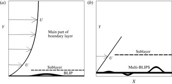
The major parts of the flow/body interaction: the short-scale flow structure which comprises a viscous–inviscid sublayer surrounded by the main part of the incident boundary layer. Here (a) is for a single blip and shows the whole boundary layer while (b) is for the corresponding configuration with several or many blips, shown closer to the wall where to leading order the incident flow is a uniform shear.

So far we have taken the time scale to respond to the inertial force. In the next section we will take it to be slower, yielding quasi-steady behaviour; the time scale
 $l^{2/3}$
reasserts itself later however through a process of intensifications.
The lower limitation in (2.2a
) corresponds to the sublayer height
 $|y|$
becoming comparable with the streamwise scale
 $\ell$
and producing a quite tiny region governed by the full system (2.1) in normalised form. In contrast the upper limitation in (2.2a
) is associated with the triple deck stage where the thin sublayer around the blip experiences a substantial feedback of pressure which arises from interaction with the flow outside the surrounding boundary layer. In between, where the range (2.2a
) applies, the sublayer is controlled by thin-layer dynamics alone. Moreover, the range of validity in (2.2a
) which is verified above is actually quite a large one in terms of the scales covered.
The flow structure is therefore concentrated primarily in the thin sublayer of figure 1. The flexible blip of unknown shape in 1(a) occupies the range
 $0<X<1$
and has height comparable with the sublayer height, whereas the surface is fixed and solid outside that range; 1(b) is for several or many blips. The blips can be humps or dents. The thick dashed line between the sublayer and the rest of the boundary layer indicates the lack of displacement over these short length scales. In the sublayer at leading order
 $$\begin{eqnarray}(u,v,p)=(\ell ^{1/3}U,\ell ^{-1/3}\mathit{Re}^{-1/2}V,\ell ^{2/3}P),\quad \text{with }x-x_{0}=\ell \,X,~y=\ell ^{1/3}\mathit{Re}^{-1/2}Y,~t=\ell ^{2/3}T,\end{eqnarray}$$
and all of the capital-lettered quantities are generally of order unity. The full system (2.1) then reduces to the well-known condensed flow interaction (Smith Reference Smith1976a ,Reference Smith b ; Smith & Daniels Reference Smith and Daniels1981) given by
 $$\begin{eqnarray}\displaystyle U={\it\Psi}_{Y},\quad V=-{\it\Psi}_{X}, & & \displaystyle\end{eqnarray}$$
 $$\begin{eqnarray}\displaystyle U_{T}+UU_{X}+VU_{Y}=-P_{X}(X,T)+U_{YY}, & & \displaystyle\end{eqnarray}$$
with the unknown scaled pressure
 $P(X,T)$
being independent of
 $Y$
because of the
 $y$
-momentum equation. The relevant boundary conditions are
 $$\begin{eqnarray}\displaystyle U=0,\quad V=\partial f/\partial T,\quad \text{at }Y=f(X,T), & & \displaystyle\end{eqnarray}$$
 $$\begin{eqnarray}\displaystyle U-{\it\lambda}Y\rightarrow 0\quad \text{as }Y\rightarrow \infty & & \displaystyle\end{eqnarray}$$
for no slip on the moving blip surface and to match with the outer flow response in turn. The requirement (2.4f
) of effectively zero displacement in
 $Y$
corresponds to the feedback effect from the flow outside the sublayer being relatively small. The function
 $f$
in (2.4d,e
) denotes the unknown scaled shape of the blip surface which is addressed further just below while the positive
 $O(1)$
factor
 ${\it\lambda}$
in (2.4f
) is the given scaled incident WSS, namely
 $\mathit{Re}^{-1/2}(\partial u/\partial y)$
at
 $y=0$
, in the surrounding boundary layer locally: see figure 1.
Concerning (second) the blip surface shape as it responds to the fluid flow over the blip, the shape and the flow interact via the local pressure as in the models used by Carpenter & Garrad (Reference Carpenter and Garrad1985), Gajjar & Sibanda (Reference Gajjar and Sibanda1996), Davies & Carpenter (Reference Davies and Carpenter1997) and Pruessner (Reference Pruessner2013) and others. The assumptions made are primarily those of the widely used membrane-model type as in the references immediately above with particularly interesting background discussions of linearly elastic materials and allied facets relevant here being in Takagi & Balmforth (Reference Takagi and Balmforth2011) as well as Vella, Kim & Mahadevan (Reference Vella, Kim and Mahadevan2004), Stewart, Waters & Jensen (Reference Stewart, Waters and Jensen2009), Singh, Lister & Vella (Reference Singh, Lister and Vella2014) and Xu, Billingham & Jensen (Reference Xu, Billingham and Jensen2014). This then gives the wall equation
 $$\begin{eqnarray}e_{1}{\it\eta}_{xxxx}+e_{2}{\it\eta}_{xx}+e_{3}{\it\eta}+e_{4}{\it\eta}_{tt}+e_{5}{\it\eta}_{t}=p-p_{0}.\end{eqnarray}$$
In this simple plate membrane model the unknown blip shape is
 $y={\it\eta}(x,t)$
and the non-dimensional constant coefficients
 $e_{n}$
are
 $(e_{1},e_{2},e_{3},e_{4},e_{5})=(-B^{\ast }/U^{\ast 2}L^{\ast 3},T_{t}^{\ast }/U^{\ast ^{2}}L^{\ast },-{\it\kappa}^{\ast }L^{\ast }/U^{\ast 2},M^{\ast }/L^{\ast },C^{\ast }/U^{\ast })/{\it\rho}^{\ast }$
with
 $M^{\ast },C^{\ast },B^{\ast },{\it\kappa}^{\ast },T_{t}^{\ast }$
being the mass density, the damping constant, the flexural rigidity, the spring stiffness and the longitudinal tension respectively, while
 $p_{0}$
is the non-dimensional base pressure relative to the oncoming pressure level which is taken to be zero. The values of the above quantities are determined experimentally or are tabulated for certain materials. The scaled version appropriate to the short-blip application is then
 $$\begin{eqnarray}\tilde{e}_{1}\,f_{XXXX}+\tilde{e}_{2}\,f_{XX}+\tilde{e}_{3}\,f+\tilde{e}_{4}\,f_{TT}+\tilde{e}_{5}\,f_{T}=P-P_{0}\end{eqnarray}$$
where
 ${\it\eta}=\mathit{Re}^{-1/2}{\it\delta}f$
,
 $\tilde{e}_{1}=\mathit{Re}^{-1/2}e_{1}/(\ell ^{4}{\it\delta})$
,
 $\tilde{e}_{2}=\mathit{Re}^{-1/2}e_{2}/(\ell ^{2}{\it\delta})$
,
 $\tilde{e}_{3}=\mathit{Re}^{-1/2}e_{3}/{\it\delta}$
,
 $\tilde{e}_{4}=\mathit{Re}^{-1/2}e_{4}/{\it\delta}^{5}$
,
 $\tilde{e}_{5}=\mathit{Re}^{-1/2}e_{5}/{\it\delta}^{3}$
,
 $P_{0}=\ell ^{-2/3}p_{0}$
. In particular
 $\tilde{e}_{1}<0$
,
 $\tilde{e}_{2}>0$
,
 $\tilde{e}_{3}<0$
. The coefficients are sensitive to the blip length scale
 $\ell$
(recall
 ${\it\delta}$
in (2.2b−f
)) and to
 $\mathit{Re}$
but in applications of interest here the dominant coefficient can sometimes be
 $\tilde{e}_{2}$
. The boundary conditions on
 $f$
are
 $$\begin{eqnarray}f=f_{X}=0\quad \text{at }X=0,1\end{eqnarray}$$
if the end points of the single blip are taken as
 $X=0,1$
for definiteness. Representative initial conditions have the shape
 $f$
and pressures
 $P,P_{0}$
being zero.
The nonlinear governing system is therefore (2.4a–f
), (2.6a,b
). Fair agreement between theoretical results based on the system and experimental results or direct simulations is found in the prescribed-shape case (Smith Reference Smith1976a
,Reference Smith
b
; Sobey Reference Sobey1980; Rothmayer & Smith Reference Rothmayer, Smith and Johnson1998). This system whether with prescribed wall shape or flexible shape then appears to require numerical treatment usually: see the next section. On the other hand if
 $P_{0}$
is zero then there is simply no disturbance. Thus, a linearised version which is also helpful and intriguing in its own right has
 $f$
being small and so (2.4a–f
) reduce to linear equations for small
 $U-{\it\lambda}Y,V,P$
. Use of a Fourier transform in
 $X$
for example as in Stewartson (Reference Stewartson1970), Smith (Reference Smith1976a
,Reference Smith
b
) and Guneratne & Pedley (Reference Guneratne and Pedley2006) along with inversion and convolution properties then yields for quasi-steady flow the integro-differential relation
 $$\begin{eqnarray}P=-{\it\gamma}\int _{0}^{X}f(s)(X-s)^{-2/3}\,\text{d}s\end{eqnarray}$$
between
 $P,f$
for
 $X>0$
, thus replacing (2.4a–f
). Here
 ${\it\gamma}=-3\,\text{Ai}^{\prime }(0){\it\lambda}^{5/3}/{\it\Gamma}(1/3)$
is a positive constant
 $\{{\approx}0.289838{\it\lambda}^{5/3}\}$
. The parabolic nature of the flow contribution on its own is then clear. Also the unknown blip
 $f$
is again assumed to start at the station
 $X=0$
for definiteness and the pressure
 $P$
there is zero. In the streamwise direction the only boundary conditions imposed on
 $U,V,P$
are at the upstream end of the first blip, where
 $U={\it\lambda}Y$
,
 $V=P=0$
, and we note that it is inappropriate to fix the downstream pressure on the current short length scales. The nature of the problem is somewhat mixed, being parabolic upstream of the blip(s), then elliptic over the length of a blip, then parabolic at all streamwise stations where there is no blip, and so on, but the overall upstream influence of a relatively long triple-deck in external flow (Stewartson Reference Stewartson1970; Smith Reference Smith1982) or the long
 $\mathit{Re}^{1/7}$
(multiplied by the channel width) axial length in internal flow (Smith Reference Smith1977; Luo & Pedley Reference Luo and Pedley1996) is insignificant for the present short blips. Likewise the corresponding flow-dominated linear instabilities existing over the longer scales are inactive in the present setting. The fully nonlinear unsteady condensed flow (2.4a
)–(2.6b
) with
 $|\partial /\partial T|$
of order unity can nevertheless lead to a finite-time breakup, Smith (Reference Smith1988) and Peridier, Smith & Walker (Reference Peridier, Smith and Walker1991), as a nonlinear by-pass into deep transition as seen later in §§ 4 and 6. The motivational settings of § 1 however are more concerned with quasi-steady behaviour initially in which
 $|\partial /\partial T|$
is relatively small.
It can be seen immediately that a positive
 $f$
shape corresponding to a bump rather than a dent provokes negative pressures, which makes sense physically in terms of an adverse pressure gradient on the front face of the blip and a favourable pressure gradient most likely on the rear face, together with a lag in the response due to convolution. Likewise a pressure rise followed by a fall is expected for a dent. The persistence of the pressure response downstream of the end point
 $X=1$
is evident from (2.7) (the integral is then from 0 to 1) and represents a wake effect. A normalisation is now applied. With
 $U,V,P,Y,T,f$
normalised by factors
 ${\it\lambda}^{m}$
where
 $m$
is
 $2/3,1/3,4/3,-(1/3),-(2/3),-(1/3)$
in turn (see the references above) and the representative
 $X$
already normalised to unity by definition of blip length, the flow contributions throughout (2.4) are thus normalised to
 $O(1)$
whereas the shape contributions in (2.6a
) have orders
 $|\tilde{e}|{\it\lambda}^{-1/3}$
on the left compared with
 ${\it\lambda}^{4/3}$
and
 $P_{0}$
successively on the right-hand side. Here only the steady case is considered for now and
 $|\tilde{e}|$
refers to the typical size of the wall coefficients
 $\tilde{e}_{n},~n=1,2,3$
, all of the wall coefficients being supposed to be of the same order for convenience. Hence the active ratios indicate two major parameters, namely
 ${\it\Gamma}_{1},{\it\Gamma}_{2}$
defined by
 $$\begin{eqnarray}\displaystyle {\it\Gamma}_{1}=P_{0}/{\it\lambda}^{4/3}\quad \text{and}\quad {\it\Gamma}_{2}=|\tilde{e}|/{\it\lambda}^{5/3}. & & \displaystyle\end{eqnarray}$$
When
 ${\it\Gamma}_{1},{\it\Gamma}_{2}$
are of order unity the fluid-shape interaction is fully nonlinear, while if
 ${\it\Gamma}_{1}$
is small then linearised theory holds since the normalised responses in
 $P,f$
become of order
 ${\it\Gamma}_{1}$
. In the subsequent calculations we tend to take
 $|\tilde{e}|$
as given as
 $O(1)$
and vary the incoming shear factor
 ${\it\lambda}$
and the relative base pressure
 $P_{0}$
in order to help explore the main two-dimensional parameter space. There are many other parameters of course detailing relative wall coefficients and blip distributions for example. The linear and nonlinear responses for a single blip are examined in the next two sections whereas those from the presence of multiple blips are addressed in § 5.
3. Results and intensifications
The influences of various physical factors are discussed in the following subsections. Analytical and numerical treatments of (2.4a–f
), (2.6a,b
) appear necessary. The numerical method we adopted is a finite difference one and, in brief, it comprises an iterative process of guessing the scaled shape
 $f$
for all
 $X$
in the range, then solving (2.4a–f
) for the scaled pressure
 $P$
or using (2.7) if applicable, then updating
 $f$
from integration of (2.6a,b
), and continuing to iterate thus between the flow and wall equations until successive iterates differ by a specified small tolerance, typically 10−6 in
 $P$
. This is with a prescribed under-pressure value
 $P_{0}$
in (2.6a
) and with a Prandtl transposition introduced into (2.4a–f
) in order to deal with the no-slip requirement accurately. The treatment applies with modifications for both the linear and the nonlinear cases, abetted by analysis in §§ 3–5, for quasi-steady slowly varying flow. Results are presented in figures 2–9. These tend to confirm the expectation from the previous section of adverse and favourable pressure gradients over the typical blip as well as corresponding reductions and increases respectively in the scaled WSS,
 $\partial U/\partial Y$
at
 $Y=0$
, along with response lags and with a clear wake effect in terms of the wall pressure downstream of the blip. Both linear and nonlinear quasi-steady flows will be considered at first below before the emphasis moves on to the linear regime for reasons (namely the occurrence of intensifications and blowups) that will become apparent.
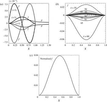
(a) Numerical results for a single blip with wall coefficients
 $[\tilde{e}_{1},\tilde{e}_{2},\tilde{e}_{3}]$
of
 $[-1,1,-1]$
, incoming shear
 ${\it\lambda}$
of unity and
 $P_{0}=1$
or
 $-1$
, showing blip shape
 $f$
, slope
 $f^{\prime }$
and fluid-flow pressure
 $P$
versus scaled distance
 $X$
. Linearised and low-amplitude nonlinear calculations are compared (light and dark). (b) As (a) but
 ${\it\lambda}$
varying from 1 to 80: linearised results for shape. (c) Normalised shape at
 ${\it\lambda}={\it\lambda}_{c}\approx 58.504$
, the first intensification value, from linearised theory.

3.1. Effects of the incident wall shear
Here the influence of the scaled wall-shear parameter
 ${\it\lambda}$
is investigated starting with figure 2(a) which shows single-blip results from the nonlinear version (2.4a–d
) with (2.6a,b
) along with those from the linearised version (2.7) with (2.6a,b
). This is for wall coefficients
 $[\tilde{e}_{1},\tilde{e}_{2},\tilde{e}_{3}]$
equal to
 $[-1,1,-1]$
, an incident shear
 ${\it\lambda}$
of unity and under-pressures
 $P_{0}$
of 1 and
 $-1$
. The versions produce almost identical results with allowance for sign changes due to
 $P_{0}$
, even though the parameter
 ${\it\Gamma}_{1}$
is not especially small here. The inference drawn tentatively is that for amplitudes that are suitably low in numerical terms the two versions can be used almost interchangeably. A subsequent result described in § 3.4 is for a raised amplitude of blip shape
 $f$
where the agreement is observed to remain close, again for wall coefficients
 $[-1,1,-1]$
. Figure 2(b) then shows how the induced shapes respond according to linearised theory when
 ${\it\lambda}$
is varied over a wide range of values with
 $P_{0}$
maintained at unity for the
 $[-1,1,-1]$
case. The rapid change of response as
 ${\it\lambda}$
passes through a critical value
 ${\it\lambda}_{c}$
between 55 and 60 is indicative of a substantial enhancement or intensification of effects then; this may be thought of as static divergence or even resonance but we refer also to the next section with respect to unsteadiness. Figure 2(c) plots the associated result from the linearised theory when
 $P_{0}$
is neglected and a renormalisation of
 $f^{\prime \prime }(0)$
to unity is applied, a result that tends to confirm an enhanced effect on shape emerging together with an eigenvalue phenomenon for
 ${\it\lambda}_{c}$
of 58.504 more precisely.
The effect of the flow on the blip shape itself (being an integral or lagged effect) is a gradual build-up with downstream distance. The blip hump rises for instance, so the induced flow pressure falls, certainly along the front face of the hump, and the scaled wall shear rises; hence this supplements the under-pressure influence tending to pull the blip surface down, with the WSS then decreasing on the leeward face of the upward blip; if the conditions are just right the interaction leads to intensification.
3.2. Effects of base pressure
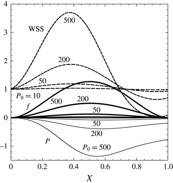
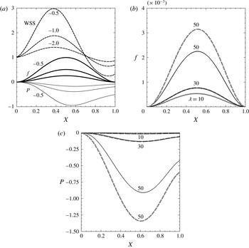
The influence of the under-pressure is investigated via figure 3, showing the blip shape, fluid pressure and WSS produced over the
 $[-1,1,-1]$
flexible blip with the incident shear
 ${\it\lambda}$
maintained at unity. The scaled under-pressures
 $P_{0}$
imposed cover a wide range from 10 to 500. Linearised properties hold well for the lower amplitudes but nonlinear effects are important at the higher amplitudes as separation in the sense of flow reversal is approached although the solutions for blip shape throughout do remain notably similar. Flow reversal is a regular phenomenon in view of the non-classical setting here, and previous solutions showing reversed-flow eddies for bumps and dents are given in figures 5–7 of Smith (Reference Smith1976a
,Reference Smith
b
), in Rothmayer & Smith (Reference Rothmayer, Smith and Johnson1998) and in Pihler-Puzović & Pedley (Reference Pihler-Puzović and Pedley2013). The results again seem physically sensible, in keeping with the earlier comments in this section.
Results for same case as in figure 2 with
 ${\it\lambda}$
of unity and
 $P_{0}$
being varied: nonlinear calculations showing
 $f,P$
, WSS (wall shear stress).

3.3. Effects of the wall coefficients
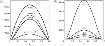
Figure 4(a) concerns the influence of the scaled wall coefficients. The calculated blip shapes
 $f$
are presented for wall coefficients
 $[\tilde{e}_{1},\tilde{e}_{2},\tilde{e}_{3}]$
such that
 $\tilde{e}_{2}$
is kept as unity but
 $\tilde{e}_{1},\tilde{e}_{3}$
are varied from
 $-1$
to zero with
 $\tilde{e}_{1},\tilde{e}_{3}$
equal, corresponding to the flexural rigidity and spring stiffness being reduced in magnitude. The under-pressure remains at unity throughout while
 ${\it\lambda}$
is also kept as unity. The responses are all at low amplitudes but the relative response in shape increases considerably as the rigidity and stiffness are reduced. We note that for all
 $[0,1,\tilde{e}_{3}]$
cases for any
 $\tilde{e}_{3}$
in the present paper only the boundary conditions of zero
 $f$
are imposed at the ends
 $X=0,1$
directly leaving
 $f^{\prime }$
to be accommodated by the implicit slight rigidity becoming significant in local end layers of relative length
 $O(|\tilde{e}_{1}|^{1/2})$
because of the higher derivatives involved. See also the variations due to wall coefficients examined in appendix A. The property that the
 $[0,1,0]$
case in particular appears comparatively remote from the other cases in figure 4(a) even at quite small rigidity and stiffness is due to the
 $|\tilde{e}_{1}|^{1/2}$
scaling. Figure 4(a) in addition shows as crosses an analytical solution brought forward from § 3.5 which is included for comparison and agrees well with the linearised numerical work. Also there is close agreement again between the nonlinear (solid) and the linearised (dashed) calculations as the figure indicates. Figure 4(b) provides a closer-in view in order to see clearly the effects from increasing the coefficients
 $\tilde{e}_{1},\tilde{e}_{3}$
in magnitude up to 2; the blip shapes reduce notably then.
Linearised shape solutions with wall coefficients
 $[\tilde{e}_{1},1,\tilde{e}_{3}],{\it\lambda}=1,P_{0}=1$
, where
 $\tilde{e}_{1}=\tilde{e}_{3}$
is varied from (a)
 $-0.1$
to 0, (b)
 $-0.1$
to
 $-2$
. A nonlinear solution is also shown by the dashed curve in (a).

Influences of increasing amplitude for different
 ${\it\lambda}$
values: (a)
 ${\it\lambda}=1$
with
 $P_{0}=200$
, wall
 $[\tilde{e}_{1},1,\tilde{e}_{3}]$
where
 $\tilde{e}_{1}=\tilde{e}_{3}$
ranges from
 $-2$
to
 $-0.5$
, nonlinear computations of
 $f,P$
, WSS; (b)
 ${\it\lambda}=10,30,50$
with
 $P_{0}=0.2$
, wall
 $[-1,1,-1]$
, comparing nonlinear (dashed curves) and linearised (solid) predictions for
 $f$
; (c) is as (b) but for
 $P$
.

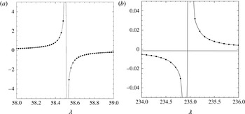
Blip height
 $f$
at midpoint
 $(X_{mid})$
as
 ${\it\lambda}$
is varied, implying enhanced responses (intensifications) near critical values
 ${\it\lambda}_{c}$
of (a) 58.5, (b) 234.9 approximately, in the
 $[-1,1,-1]$
case with
 $P_{0}$
of unity.

3.4. Increasing amplitudes
Figure 5(a–c) addresses further the effects of scaled amplitudes and provides evidence of two distinct paths into nonlinear behaviour, one standard and one not. Variations in the wall coefficients similar to those of figure 4(a,b) are examined in figure 5(a) but with
 $P_{0}$
increased to 200, which raises the blip amplitudes firmly into the nonlinear range and shows a trend towards flow reversal taking place just ahead of the downstream end of the blip. Phenomena similar to those in § 3.2 thus occur here including induced adverse pressure gradients near the rear of the blip. Figure 5(b) examines a less familiar trend, for the basic
 $[-1,1,-1]$
case with base pressure
 $P_{0}$
reduced to 0.2 but increasing
 ${\it\lambda}$
. The resulting blip shapes for a given
 ${\it\lambda}$
from linear and nonlinear calculations remain almost graphically indistinguishable from each other up to
 ${\it\lambda}$
values of 30 or so but the differences begin to show up clearly when
 ${\it\lambda}$
is increased to about 50; these herald the approach to intensification as
 ${\it\lambda}\rightarrow {\it\lambda}_{c}\;({\approx}58.504\text{ in this case})$
. Lowering the base pressure delays the onset of these differences. The same trend occurs in the corresponding pressures shown in figure 5(c).
3.5. Intensification
The effects observed intensify according to the computational results above as certain critical parameter values are approached. See also the plots in figures 6–9 concerning among other quantities the critical
 ${\it\lambda}$
values for full intensification. Figure 6(a,b) is for the basic case of
 $[-1,1,-1],P_{0}$
of unity, but with
 ${\it\lambda}$
varying more widely: see also figures 2(b,c), 5(b,c). Now another intensification is indicated clearly near a higher
 ${\it\lambda}$
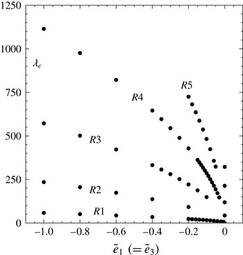
value of about 235, i.e. a second eigenvalue. Figure 7 presents the critical values
 ${\it\lambda}_{c}$
plotted against
 $\tilde{e}_{1}\;(=\tilde{e}_{3})$
obtained for 4–5 successive roots by treating (2.6a,b
), (2.7) as a shooting problem with the constant
 $P_{0}$
omitted. The trend is one of increasing
 ${\it\lambda}_{c}$
overall as the rigidity and stiffness are increased, for a given root number, while the remoteness between critical values for nominally zero rigidity and stiffness parameters and small parameter values is in line with the
 $|\tilde{e}|^{1/2}$
scaling described in § 3.3. The close-in results suggest that each root for zero rigidity and stiffness may propagate more than one set of roots
 $R1,R2$
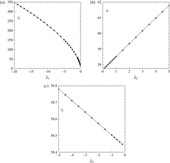
and so on among those shown for non-zero rigidity and stiffness. In figure 8(a–c) by contrast we show the first-root eigenvalues associated with intensification for cases where each of
 $\tilde{e}_{1},\tilde{e}_{2},\tilde{e}_{3}$
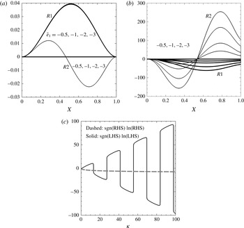
is varied separately in order to present a different slice through the parameter space, which connects with the parameter study in appendix A and accompanying analysis. Next, figure 9(a,b) gives plots of the shapes
 $f$
and induced pressures
 $P$
from both the first and second roots in wall cases
 $[\tilde{e}_{1},1,-1]$
with the coefficient
 $\tilde{e}_{1}$
being varied between
 $-0.5$
and
 $-3$
. We see little change in
 $f$
over the range for a given set of first or second roots whereas the pressure
 $P$
alters considerably for each set, which is physically sensible because of the different incident shear values, and the maximum magnitude of the pressure depends almost linearly on
 $\tilde{e}_{1}$
. Shown in figure 9(c) is a plot relevant to the special case of
 $[0,1,0]$
described at the end of the current section and confirming the existence of multiple roots.
Intensification roots for varying wall coefficients. Roots
 ${\it\lambda}_{c}$
versus
 $\tilde{e}_{1}\;(=\tilde{e}_{3})$
showing roots
 $R1$
–
 $R5$
for cases
 $[\tilde{e}_{1},1,\tilde{e}_{3}]$
.

Intensifications for wall coefficients
 $[\tilde{e}_{1},1,-1],[-1,\tilde{e}_{2},-1],[-1,1,\tilde{e}_{3}]$
respectively. First roots
 ${\it\lambda}_{c}$
are plotted against
 $\tilde{e}_{1},\tilde{e}_{2},\tilde{e}_{3}$
in turn.

(a) Renormalised shapes
 $f$
versus
 $X$
at the first and second roots for cases
 $[\tilde{e}_{1},1,-1]$
with various
 $\tilde{e}_{1}$
. (b) As (a), showing pressure
 $P$
. (c) Case
 $[0,1,0]$
: right- and left-hand sides (RHS, LHS) of (3.4a
) in logarithmic form plotted against
 ${\it\kappa}$
; their crossings identify the intensification roots.

Additional analytical support can be given in regard to intensification and a succession of critical values. In the linear regime first, formally, an exponential solution proportional to
 $\exp (mX)$
applies at large
 $X$
values downstream or for rapid spatial variation if
 $X$
is renormalised to keep
 $f^{\prime \prime }(0)=1$
, the
 $\tilde{e}_{n}$
coefficients are adjusted accordingly,
 $n=1,2,3$
, and shooting forward in
 $X$
from zero
 $f,f^{\prime }$
at zero
 $X$
with a single parameter is considered. This supplements a particular solution proportional to
 $P_{0}$
. The unknown exponential factor
 $m$
must satisfy
 $$\begin{eqnarray}\tilde{e}_{1}m^{4}+\cdots =-\bar{{\it\gamma}}m^{1/3},\end{eqnarray}$$
where
 $\bar{{\it\gamma}}$
is proportional to
 ${\it\gamma}$
and depends on the renormalisation. The relation (3.1) allows oscillatory behaviour which can be adjusted in principle to give
 $f,f^{\prime }$
zero at the end
 $X=1$
. Second, suppose that the governing equation (2.6a
) is dominated by the contribution involving
 $\tilde{e}_{2}$
on the left. Then the derivative conditions in (2.6b
) have to be abandoned and the small-
 $X$
expansion of
 $f$
has the form
 $$\begin{eqnarray}f=a_{1}X+a_{2}X^{{\it\omega}}+\cdots\end{eqnarray}$$
where
 ${\it\omega}$
is
 $10/3$
with
 $a_{1}$
unknown but
 $a_{2}=-81{\it\gamma}a_{1}/(280\tilde{e}_{2})$
, for the case of zero
 $P_{0}$
. If the condition
 $f=0$
is then imposed at
 $X=1$
the approximate requirement
 $a_{1}+a_{2}=0$
is obtained. Hence there is a non-trivial solution for
 $$\begin{eqnarray}{\it\gamma}\approx \left({\textstyle \frac{280}{81}}\right)\tilde{e}_{2},\end{eqnarray}$$
as an estimate for intensification. Extending this to include non-zero wall coefficients
 $\tilde{e}_{3}$
and base pressures
 $P_{0}$
leads to the relation
 $$\begin{eqnarray}[1-81{\it\gamma}/(280\tilde{e}_{2})-\tilde{e}_{3}/(6\tilde{e}_{2})]a_{1}=P_{0}/(2\tilde{e}_{2}),\end{eqnarray}$$
for the constant
 $a_{1}$
, away from the intensification at a critical value
 ${\it\lambda}={\it\lambda}_{c}$
,
 ${\it\gamma}_{c}=(0.289838\dots ){\it\lambda}_{c}^{5/3}=280\tilde{e}_{2}(1-\tilde{e}_{3}/(6\tilde{e}_{2}))/(81)$
wherever the term in square brackets on the left is zero in (3.2c
). The prediction (3.2c
) has the effective slope
 $a_{1}$
and base pressure
 $P_{0}$
being of identical sign for
 ${\it\lambda}$
values below critical and opposite signs above critical, in line with the numerical results in figures 2(b), 6–9. A similar analysis based on the
 $\tilde{e}_{1}$
contribution dominating leads to
 ${\it\omega}$
being
 $16/3$
and the estimate
 ${\it\gamma}\approx (58\,240/729)\tilde{e}_{1}$
for intensification which is closer to the numerical values obtained.
In the (third) special case of small or negligible
 $\tilde{e}_{1},\tilde{e}_{3}$
a Laplace-transform approach as in Pruessner (Reference Pruessner2013) provides an explicit solution in the form
 $$\begin{eqnarray}{\it\kappa}\tilde{e}_{2}f(X)=\frac{6}{7}\text{e}^{{\it\nu}_{1}X}\left[{\it\alpha}\cos {\it\alpha}_{1}-\frac{P_{0}}{{\it\kappa}}\cos {\it\beta}_{1}\right]-\frac{3^{1/2}}{2{\rm\pi}}\int _{0}^{\infty }\frac{({\it\alpha}+P_{0}{\it\kappa}^{-1}R^{-1})R^{1/3}e^{-{\it\kappa}RX}\,\text{d}R}{\hat{D}},\end{eqnarray}$$
where
 ${\it\kappa}\equiv \tilde{{\it\gamma}}^{3/7}$
,
 ${\it\alpha}_{1}\equiv 3{\rm\pi}/7-{\it\nu}_{2}X$
,
 ${\it\beta}_{1}\equiv 6{\rm\pi}/7-{\it\nu}_{2}X$
,
 ${\it\nu}_{1}\equiv {\it\kappa}\sin 3{\rm\pi}/7$
,
 ${\it\nu}_{2}\equiv {\it\kappa}\cos 3{\rm\pi}/7$
,
 $\tilde{{\it\gamma}}\equiv {\it\gamma}{\it\Gamma}(1/3)/\tilde{e}_{2}$
are given while
 ${\it\alpha}\equiv \tilde{e}_{2}\,f^{\prime }(0)$
is unknown. Also
 $\hat{D}=(R^{14/3}+R^{7/3}+1)$
. The condition
 $f(1)=0$
then acts to determine
 ${\it\alpha}$
since, from (3.3a
),
 $$\begin{eqnarray}D_{1}{\it\alpha}+D_{2}P_{0}=0,\end{eqnarray}$$
with the coefficients
 $D_{1},D_{2}$
defined by
 $$\begin{eqnarray}\displaystyle & \displaystyle {\it\kappa}D_{1}=\frac{3^{1/2}}{2{\rm\pi}}\int _{0}^{\infty }\frac{R^{1/3}\text{e}^{-{\it\kappa}R}\,\text{d}R}{\hat{D}}-\frac{6}{7}\text{e}^{{\it\nu}_{1}}\cos \left(\frac{3{\rm\pi}}{7}-{\it\nu}_{2}\right), & \displaystyle\end{eqnarray}$$
 $$\begin{eqnarray}\displaystyle & \displaystyle {\it\kappa}^{2}D_{2}=\frac{3^{1/2}}{2{\rm\pi}}\int _{0}^{\infty }\frac{R^{-2/3}\text{e}^{-{\it\kappa}R}\,\text{d}R}{\hat{D}}+\frac{6}{7}\text{e}^{{\it\nu}_{1}}\cos \left(\frac{6{\rm\pi}}{7}-{\it\nu}_{2}\right). & \displaystyle\end{eqnarray}$$
A comparison with the numerical results above is favourable and is shown in figure 4(a) concerning the blip shape. Moreover the roots or eigenvalues at which intensification occurs are given simply by
 $$\begin{eqnarray}\frac{3^{1/2}}{2{\rm\pi}}\int _{0}^{\infty }\frac{R^{1/3}\text{e}^{-{\it\kappa}R}\,\text{d}R}{\hat{D}}=\frac{6}{7}\text{e}^{{\it\theta}_{1}{\it\kappa}}\cos \left(\frac{3{\rm\pi}}{7}-{\it\theta}_{2}{\it\kappa}\right),\end{eqnarray}$$
from (3.3a,b
), in this special case. Here
 ${\it\theta}_{1}=\sin 3{\rm\pi}/7$
,
 ${\it\theta}_{2}=\cos 3{\rm\pi}/7$
are constants. The relation (3.4a
) establishes that there are infinitely many intensification roots
 ${\it\kappa}={\it\kappa}_{n}$
successively, and
 $$\begin{eqnarray}{\it\kappa}_{n}\sim \left.\left(n+\frac{{\rm\pi}}{14}\right)\!\right/{\it\theta}_{2}\end{eqnarray}$$
at large
 $n$
. The dominant roots stemming from (3.4a
) are presented in terms of the predictions for the critical
 ${\it\lambda}$
values in figure 9(c) and they agree closely with the large-
 $n$
asymptote (3.4b
) even for
 $n$
of unity. We remark that although at first glance a
 ${\it\lambda}$
of zero might appear to be a root it is not really so for this case; it just corresponds to the value
 $f(0)$
being zero as required. The approach can be extended to general wall coefficients, and we note in addition that for small non-zero
 $\tilde{e}_{3}$
values the roots lie close to those of (3.4a
) whereas for small nonzero
 $\tilde{e}_{1}$
some roots lie there but others arise at large values of the Laplace-transformed variable corresponding to short-length effects concentrated near the endpoints at
 $X=0,1$
usually. These and the previous results indicate that nonlinear influences, for example in § 3.4 and figure 5(a–c), and the closeness to intensification, where the amplitude
 $|f|$
grows in inverse proportion to
 $|{\it\lambda}-{\it\lambda}_{c}|$
according to either (3.2c
) or (3.3a
), must have an interesting interplay.
4. Weakly nonlinear behaviour of a single blip near intensification
To clarify how nonlinearity first affects intensification at low amplitude this section considers the weakly nonlinear response of the blip shape and the local flow properties at parameter values close to a typical intensification. Near a representative critical value
 ${\it\lambda}_{0}$
for intensification the scaled incident WSS can be expressed as
 $$\begin{eqnarray}{\it\lambda}={\it\lambda}_{0}+{\it\epsilon}{\it\lambda}_{1}+\cdots\end{eqnarray}$$
say, where the constant
 ${\it\epsilon}$
is small and the coefficients
 ${\it\lambda}_{0},{\it\lambda}_{1}$
and so on are of order unity. The entire fluid-body interaction then takes the form
 $$\begin{eqnarray}\displaystyle \{U,{\it\Psi},P\} & = & \displaystyle \{{\it\lambda}_{0}Y,{\textstyle \frac{1}{2}}{\it\lambda}_{0}Y^{2},0\}+{\it\epsilon}\{AU_{1}+{\it\lambda}_{1}Y,A{\it\Psi}_{1}+{\textstyle \frac{1}{2}}{\it\lambda}_{1}Y^{2},AP_{1}\}\nonumber\\ \displaystyle & & \displaystyle +\,{\it\epsilon}^{2}\{U_{2},{\it\Psi}_{2},P_{2}\}+\cdots \,,\end{eqnarray}$$
 $$\begin{eqnarray}\displaystyle \{f,P_{0}\} & = & \displaystyle {\it\epsilon}\{Af_{1},0\}+{\it\epsilon}^{2}\{f_{2},P_{02}\}+\cdots \,,\end{eqnarray}$$
 $$\begin{eqnarray}\displaystyle \tilde{e}_{M} & = & \displaystyle \tilde{e}_{1M}+{\it\epsilon}\tilde{e}_{2M}+\cdots\end{eqnarray}$$
 $M=1,2,3$
, when nonlinear influences first become substantial. The blip-shape perturbation of order
 ${\it\epsilon}$
is an order of magnitude greater than the base-pressure perturbation (of order
 ${\it\epsilon}^{2}$
) in (4.2b
), hence providing evidence of the occurrence of intensification subject to the self-consistency that emerges below. The critical disturbance function
 $f_{1}$
is taken to be normalised such that
 $f_{1}^{\prime \prime }(0)=1$
, for the sake of definiteness, whereas
 $A$
represents the unknown disturbance amplitude and is dependent on the slow scaled time
 $\tilde{T}$
in general which is defined by time
 $T={\it\epsilon}^{-1}\tilde{T}$
. The physical expectation is that the slow-time dependence is present usually because of variations in the under-pressure or in the change in the wall-shear factor
 ${\it\lambda}_{1}$
, while the leading factor
 ${\it\lambda}_{0}$
must normally remain constant for physical sense in the scalings. If
 ${\it\lambda}$
is evolving faster, on the condensed scale with
 $T$
of
 $O(1)$
, then the far-field conditions involve a Stokes layer (Brown & Daniels Reference Brown and Daniels1975) wherein
 $Y$
is
 $O(1)$
balancing the order of magnitude
 $T^{1/2}$
from (2.4d,e
) at large
 $|X|$
. For slow evolutions however the effective time scale is larger and so is the Stokes
 $Y$
scale, even lying outside the condensed layer of § 2 if the effective time scale is as large as a positive power of
 $\mathit{Re}$
. Further the evolution in (4.1)–(4.2c
) is with regard to the perturbation in
 ${\it\lambda}$
rather than the leading-order contribution. A weak temporal dependence through the additional wall-flexibility coefficients
 $\tilde{e}_{4},\tilde{e}_{5}$
in (2.6a
) would also be admissible and is discussed later in § 6 but we focus here on temporal dependence springing from the fluid-dynamical background. The relative smallness of the under-pressure in (4.2b
) is notable, its order-
 ${\it\epsilon}^{2}$
size being due to the interaction intensifying at the leading order
 ${\it\epsilon}$
. Further the contributions to the wall-flexibility parameters of order
 ${\it\epsilon}$
and smaller on the right-hand side of (4.2c
) correspond to detuning of the intensification; a similar effect can be generated by slight detuning of the blip length.
Substitution of (4.1)–(4.2c
) into the nonlinear governing equations (2.4a–f
), (2.6a,b
) along with the usual stream-function properties yields at leading order
 $O({\it\epsilon})$
the unforced linear system
 $$\begin{eqnarray}\displaystyle & U_{mX}+V_{mY}=0, & \displaystyle\end{eqnarray}$$
 $$\begin{eqnarray}\displaystyle & {\it\lambda}_{0}YU_{mX}+V_{m}{\it\lambda}_{0}=-P_{mX}+U_{mYY}+R_{1m}, & \displaystyle\end{eqnarray}$$
 $$\begin{eqnarray}\displaystyle & \text{with }U_{m}\sim {\it\lambda}_{0}f_{m}+R_{2m}\quad \text{as }Y\rightarrow \infty , & \displaystyle\end{eqnarray}$$
 $$\begin{eqnarray}\displaystyle & U_{m}=V_{m}=0\quad \text{at }Y=0, & \displaystyle\end{eqnarray}$$
 $$\begin{eqnarray}\displaystyle & \tilde{e}_{11}\,f_{m}^{\prime \prime \prime \prime }+\tilde{e}_{21}\,f_{m}^{\prime \prime }+\tilde{e}_{31}\,f_{m}=P_{m}+R_{3m}, & \displaystyle\end{eqnarray}$$
 $m$
is unity and
 $R_{11}$
–
 $R_{31}$
are identically zero. Here
 $X$
lies between
 $0,1$
, the values of
 $f_{m},f_{m}^{\prime }$
are to be zero at the end points and the intensification or eigen-function which is accentuated through the absence of any forcing on the
 $m=1$
quantities is described below. At next order,
 $O({\it\epsilon}^{2})$
, the same system applies but with
 $m=2$
and with the forcing that arises from detuning, evolutionary and nonlinear contributions, so that
 $$\begin{eqnarray}\displaystyle & R_{12}=-\text{d}A/\text{d}\tilde{T}U_{1}-A{\it\lambda}_{1}(YU_{1X}+V_{1})-A^{2}(U_{1}U_{1X}+V_{1}U_{1Y}), & \displaystyle\end{eqnarray}$$
 $$\begin{eqnarray}\displaystyle & R_{22}=A{\it\lambda}_{1}f_{1}, & \displaystyle\end{eqnarray}$$
 $$\begin{eqnarray}\displaystyle & R_{32}=-P_{02}-A(\tilde{e}_{12}\,f_{1}^{\prime \prime \prime \prime }+\tilde{e}_{22}\,f_{1}^{\prime \prime }+\tilde{e}_{32}\,f_{1}). & \displaystyle\end{eqnarray}$$
 $R_{12},R_{22}$
are flow-field effects while
 $R_{32}$
constitutes the wall effect.
The solution of (4.3a–e
) may be obtained by means of a Fourier transform (superscripted
 $F$
) applied in
 $X$
, which allows (4.3a,b
) to be cast as a forced Airy equation for the scaled flow shear. Hence,
 $$\begin{eqnarray}(\partial u_{m}/\partial y)^{F}=[(\text{i}{\it\alpha}{\it\lambda}_{0})^{-1/3}I({\it\xi})+B_{m}]\text{Ai}({\it\xi})\end{eqnarray}$$
where
 ${\it\alpha}$
is the transform variable,
 $\text{Ai}$
is the Airy function,
 ${\it\xi}=(\text{i}{\it\alpha}{\it\lambda}_{0})^{1/3}Y$
and
 $$\begin{eqnarray}I({\it\xi})=\int _{0}^{{\it\xi}}(\text{Ai}(\hat{q}))^{-2}\left[\int _{\infty }^{q}\text{Ai}(\hat{{\it\xi}})R_{1m\hat{{\it\xi}}}^{F}\,\text{d}\hat{{\it\xi}}\right]\text{d}\hat{q}.\end{eqnarray}$$
Use of (4.3c,d
) then enables the unknown shear constant
 $B_{m}$
to be determined in terms of the scaled pressure which is found to be given by
 $$\begin{eqnarray}P_{m}^{F}=3{\it\lambda}_{0}^{5/3}(\text{i}{\it\alpha})^{-1/3}\text{Ai}^{\prime }(0)f_{m}^{F}+{\it\Gamma}^{F}.\end{eqnarray}$$
Here
 $$\begin{eqnarray}(\text{i}{\it\alpha}){\it\Gamma}^{F}=-\text{Ai}(0)I^{\prime }(0)+3\text{Ai}^{\prime }(0)\left\{\int _{0}^{\infty }\text{Ai}({\it\xi})I({\it\xi})\,\text{d}{\it\xi}+(\text{i}{\it\alpha})^{2/3}{\it\lambda}_{0}^{2/3}R_{2m}^{F}\right\}.\end{eqnarray}$$
So the wall balance (4.3e ) requires the relation
 $$\begin{eqnarray}\tilde{e}_{11}\,f_{m}^{\prime \prime \prime \prime }+\tilde{e}_{21}\,f_{m}^{\prime \prime }+\tilde{e}_{31}\,f_{m}=-{\it\gamma}\int _{0}^{X}f_{m}(s)(X-s)^{-2/3}\,\text{d}s+R_{42}(X)\end{eqnarray}$$
to hold, in which
 $R_{42}(X)={\it\Gamma}(X)+R_{32}(X)$
. The factor multiplying the integral on the right in (4.7a
) agrees with the intensified value of that in (2.7) as required for consistency. The relation (4.7a
), which is subject to the end conditions
 $$\begin{eqnarray}f_{m}=f_{m}^{\prime }=0\quad \text{at }X=0,1,\end{eqnarray}$$
acts at leading order
 $(m=1)$
to define the intensified blip shape in normalised form but also acts, at the second order
 $(m=2)$
where the
 $R$
terms are non-zero, to provide a solvability constraint that helps control the unknown amplitude. This constraint stems from use of the normalised function
 $q(X)$
say that is adjoint to
 $f_{1}(X)$
and can be shown from (4.7a,b
) when
 $m=1$
to be given by
 $q(X)=f_{1}(1-X)$
. Multiplication through by
 $q(X)$
in (4.7a
) when
 $m=2$
then leads to the requirement that
 $$\begin{eqnarray}\int _{0}^{1}R_{42}(X)q(X)\,\text{d}X=0\end{eqnarray}$$
which constitutes an amplitude equation. A substitution of the effects from (4.4a–c
) in the requirement (4.8) yields the amplitude equation for
 $A(\tilde{T})$
as
 $$\begin{eqnarray}d_{1}\frac{\text{d}A}{\text{d}\tilde{T}}+d_{7}A+d_{6}A^{2}+P_{02}=0,\end{eqnarray}$$
where
 $$\begin{eqnarray}d_{7}\equiv d_{2}{\it\lambda}_{1}+d_{3}\tilde{e}_{12}-d_{4}\tilde{e}_{22}+d_{5}\tilde{e}_{32}\end{eqnarray}$$
and it can be shown that all the coefficients
 $d_{1}{-}d_{6}$
are positive; a calculation gives the estimates
 $0.422,0.392,14.76,0.362,0.029,1.11$
in turn. The latter values are for the central example of the wall coefficients
 $\tilde{e}_{1},\tilde{e}_{2},\tilde{e}_{3}$
being
 $-1,1,-1$
respectively whereas effects over a wide range of variation in these wall coefficients are investigated in appendix A.
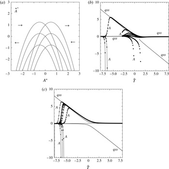
(a) The phase-plane solution with horizontal axis
 $A^{\ast }=d_{6}A/|d_{7}|$
and vertical
 $\stackrel{\bullet }{A}^{\ast }$
for times
 $|d_{7}|\tilde{T}/d_{1}$
, associated with weakly nonlinear evolution in or near intensification. (b) Evolution of amplitude
 $A$
when
 $d_{7}=\tilde{T},P_{02}=0.25$
with
 $d_{1},d_{6}$
normalised to unity, for various small kicks in amplitude at large negative
 $\tilde{T}$
. Quasi-steady states denoted
 $\mathit{qss}$
are shown for comparison. (c) As (b) but
 $P_{02}=-0.25$
.

The amplitude equation (4.9a
) encapsulating the nonlinear response in terms of the amplitude function
 $A(\tilde{T})$
is Riccati-like and yields the phase-plane diagram drawn in figure 10(a), when
 $d_{1},d_{6},d_{7}$
are independent of time
 $\tilde{T}$
, which tends to confirm the significance of only the signs of the coefficients above. Varying the scaled pressure
 $P_{02}$
yields the different sets of trajectories with positive, zero or negative intercept values (
 $+,0,-$
respectively) at zero
 $A$
while
 $d_{7}$
being positive or negative is responsible for the left–right reflection of the curves. Here
 $d_{7}$
may be positive or negative depending on the four parts which constitute that coefficient. The arrows indicate direction along the trajectories with increasing time: rightwards in the upper half plane and leftwards in the lower half. The normalised diagram, plotting
 $(d_{6}d_{1}/|d_{7}|^{2})\,\text{d}A/\text{d}\tilde{T}$
against
 $d_{6}A/|d_{7}|$
, shows first that if the scaled under-pressure
 $P_{02}$
is negative then on any solution trajectory there are two roots of the quadratic equation corresponding to zero time derivative, one root having positive amplitude and the other negative, and all trajectories are also connected with a large-amplitude asymptote in which
 $\text{d}A/\text{d}\tilde{T}\propto A^{2}$
with a negative coefficient of proportionality. On the other hand if
 $P_{02}$
is positive then two roots are found if
 ${d_{7}}^{2}>4d_{6}P_{02}$
(in which case the roots are of the same sign), one root in the marginal case where equality holds and no real roots otherwise. Again the connection with a large-amplitude asymptote is clear. Whether the under-pressure is positive or negative, the greater of the two amplitude roots acts as an attractor and the lesser one as a repellor whenever two roots exist, whereas the large-amplitude asymptote which is featured on the left-hand side of the diagram with
 $A$
tending to negative infinity serves as an attractor in every instance. The initial value of
 $A$
and subsequent evolution with scaled time can play a key role in deciding the eventual outcome for the evolving amplitude. The choice of outcomes is
 $$\begin{eqnarray}\displaystyle & A\rightarrow [-d_{7}+({d_{7}}^{2}-4d_{6}P_{02})^{1/2}]/(2d_{6})\quad \text{as }\tilde{T}\rightarrow \infty ,\text{ for }{d_{7}}^{2}>4d_{6}P_{02}, & \displaystyle\end{eqnarray}$$
 $$\begin{eqnarray}\displaystyle & A\sim -(d_{1}/d_{6})(\tilde{T}_{0}-\tilde{T})^{-1}\quad \text{as }\tilde{T}\rightarrow \tilde{T}_{0}-. & \displaystyle\end{eqnarray}$$
 $P_{02}$
and the coefficient
 $d_{7}$
, and is consistent with the value
 $-P_{02}/(d_{2}{\it\lambda}_{1})$
for the linear steady regime and results of § 3 when
 ${\it\lambda}$
approaches the critical value identified there with prescribed
 $\tilde{e}_{n}$
coefficients. This links with the quasi-steady behaviour of § 3 at low amplitudes.
In contrast the blow-up behaviour in (4.10b
) occurs at a finite scaled time and is such that the fully nonlinear system (2.4a–f
), (2.6a,b
) is reinstated over a shorter time scale around the blow-up time
 $T$
of approximately
 ${\it\epsilon}^{-1}\tilde{T}_{0}$
. This is because when
 $T-{\it\epsilon}^{-1}\tilde{T}_{0}$
becomes of order unity the denominator in (4.10b
) becomes of order
 ${\it\epsilon}$
, making
 $A$
grow as large as
 ${\it\epsilon}^{-1}$
and therefore causing the
 $U$
-perturbation and
 $|f|$
in (4.2a,b
) to become of order unity. Saturation as in (4.10a
) and blow-up to full (strong) nonlinearity within a finite scaled time as in (4.10b
) are the two main possibilities for the weakly nonlinear near-intense response, then, while the latter full nonlinearity leads on to the strong break-up route discussed later in terms of transition.
Concerning (4.9a,b
) further the results in figure 10(b,c) are formally for varying
 ${\it\lambda}_{1}$
from large negative to large positive values which force
 $d_{7}$
to pass smoothly from negative to positive; specifically this is normalised to
 $d_{7}=\tilde{T}$
with
 $d_{1}=d_{6}=1$
. The scaled base pressure is
 $\pm 0.25$
. The low-amplitude asymptotes for large negative times
 $\tilde{T}$
match with the quasi-steady behaviour found in § 3 whereas blow-up of the amplitude
 $A$
can be produced within a finite time, confirming the nonlinear progression to the strong break-up route mentioned at the conclusion of the previous paragraph.
5. Intensifications for many blips
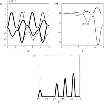
Interactive solutions for multi-blips are now considered. Solutions for four blips are presented in figure 11(a,b), with the values of the wall coefficients fixed at
 $(-1,1,-1)$
. These are linear results. Also solutions for one, two or three blips correspond to terminating the calculation just before the second, third or fourth blip successively. In figure 11(a) two different arrangements of the four under-pressures are considered, for parameter
 ${\it\lambda}$
of unity, and it is apparent that the interactions between the successive blips are relatively mild in these cases. In figure 11(b)
 ${\it\lambda}$
is increased to a near-critical value of 55 where the interactions are seen to be considerable. When
 $P_{0}$
is positive the minimum pressure produced decreases with downstream distance
 $X$
and the maximum pressure also decreases, and in addition the scaled pressure
 $P$
starts from a non-zero value at the beginning of all but the first blip because of the wake effect. For linear or nonlinear intensifications the wake effects in the induced pressure field can play a substantial role in the total interaction produced by a configuration of many blips, as described below.
Two or more blips. (a) Linearised
 $f,P$
versus
 $X$
with successive base-pressures
 $P_{0}$
of
 $1,1,1,1$
(thin curves) or
 $1,-1,1,-1$
(thick), blip lengths unity,
 ${\it\lambda}=1$
, wall case
 $[-1,1,-1]$
. (b) Linearised
 $f,P$
with base pressures
 $1,1,1,1$
, blip lengths unity,
 ${\it\lambda}=55$
(just below intensification), wall case
 $[-1,1,-1]$
. (c) Weakly nonlinear heights
 $f$
for the equimaterial setting of (5.1), equally or unequally spaced blips, yielding heights
 ${\it\epsilon},{\it\epsilon}^{1/2}$
, etc., as
 $X$
increases; not to scale. Results for 2 blips stop before the third, 3 blips stop before the fourth, and so on.

Sketch, not to scale, of effects of changing incident shear
 ${\it\lambda}$
: curve
 $a$
shows response of max
 $|WSS|$
if
 ${\it\lambda}$
varies slowly as in
 $b$
from subcritical to supercritical; when
 ${\it\lambda}$
variation is instead as in
 $c$
the response remains close to
 $c$
. Time scales (i)–(iv),… are slow, fast, faster, faster, ….

Supposing the configuration consists of a sequence of blips that are of identical length (normalised to unity), identical material and so on, but not necessarily spaced out equally, we consider the most upstream one first. This approach ties in with the mixed parabolic–elliptic nature of the entire fluid/body interaction. Near or in intensifications the first blip produces a dominant scaled pressure response
 $P$
and scaled shape response
 $F$
which in the incipient nonlinear range have amplitude of order
 ${\it\epsilon}$
, that is small as in § 4, and these act as eigenfunctions. The associated under-pressure
 $P_{0}$
is only of order
 ${\it\epsilon}^{2}$
then and acts at second order to help control the detailed amplitude evolution; thus, the dominant pressure response varies as the square root of the forcing pressure. The main point now concerns the
 $O({\it\epsilon})$
pressure
 $P$
and the fact that it exhibits a wake contribution as referred to in § 3, a contribution which extends over the second blip in particular. As a consequence the forcing pressure for the second blip is also of
 $O({\it\epsilon})$
. Moreover this blip is augmented, as it is identical to the first blip, and so it produces the very same eigenfunction response as before except that, crucially, the amplitude is of order
 ${\it\epsilon}^{1/2}$
since the forcing pressure (replacing under-pressure effect) is now of order
 ${\it\epsilon}$
. The overall effect is therefore larger on the second blip and begins as if anew. Also the mechanism can continue afresh to further blips downstream: the pressure wake effect from the second blip is
 $O({\it\epsilon}^{1/2})$
, extends over the third blip, produces
 $O({\it\epsilon}^{1/4})$
amplitudes in pressure and shape on the third blip; the pressure wake effect from the third blip is
 $O({\it\epsilon}^{1/4})$
, extends over the fourth blip, produces
 $O({\it\epsilon}^{1/8})$
amplitudes in pressure and shape there; and so on.
The prediction then is of an increasing trend of pressure and shape amplitudes with increasing distance downstream, and likewise for the wall-shear perturbations. The trend has the enhanced amplitude sequence:
 $$\begin{eqnarray}{\it\epsilon},{\it\epsilon}^{1/2},{\it\epsilon}^{1/4},{\it\epsilon}^{1/8},{\it\epsilon}^{1/16},\dots\end{eqnarray}$$
from blip to successive blip for the above case of several identically constituted blips (see figure 11 c) whereas for example the sequence is
 $$\begin{eqnarray}{\it\epsilon},{\it\epsilon}^{1/2},{\it\epsilon}^{1/2},{\it\epsilon}^{1/2},{\it\epsilon}^{1/4},\dots\end{eqnarray}$$
for the case of two identical blips followed by any two differently constituted blips and then identical ones again. Each of the two different blips here provokes a maintained amplitude in shape and pressure because of the wake-pressure effect from its immediate predecessor and so delays the enhancement but does not prevent it continuing downstream. Overall, the increasing downstream trend and mechanism involved seem to add weight to the significance of non-periodicity in the overall configuration.
The same or similar reasoning extends to configurations other than the identical-blips one above, as (5.2) indicates. A combination of the workings in this and the previous sections points to a succession of linked nonlinear amplitude equations which are of considerable interest for future research.
6. Further comments
Three points (i)–(iii) stand out in conclusion.
(i) Inferences on flow transition. The work has shown that when the wall shear of the incident boundary layer flow acquires certain critical values (eigenvalues) a tiny flexible blip can, after some delay, rise or fall to a magnitude much greater than is otherwise the case. This intensification (§ 3, § 5) along with blowup (§ 4 and see next paragraph) points to a tuneable trip being feasible over a wide parameter range in the boundary layer. Both shear and wall flexibility are required for the present intensifications and fast growth mechanisms to occur as the present scales lie outside the usual boundary-layer instability of Tollmien–Schlichting waves (Smith Reference Smith1979).
Intensification leads to a non-standard path into transition from low amplitudes, as figure 12 indicates by showing schematically the effects of gradually changing the oncoming shear
 ${\it\lambda}$
for the regime of relatively low base pressures. Curve
 $a$
shows the response of the maximal
 $|WSS|$
when
 ${\it\lambda}$
varies slowly as in
 $b$
from subcritical to supercritical. The response produces only a small disturbance from
 ${\it\lambda}$
over the quasi-steady temporal scale (i) of § 3 until a critical value
 ${\it\lambda}={\it\lambda}_{c}$
is encountered at which stage (ii) weakly nonlinear amplification can occur (§ 4), leading to strongly nonlinear evolution over the faster time scale (iii) of (2.4a–f
), (2.6a,b
). This is followed by finite-time blowup as in Smith (Reference Smith1988) and Peridier et al. (Reference Peridier, Smith and Walker1991) which provokes the even faster evolution (iv) described by Davies, Bowles & Smith (Reference Davies, Bowles and Smith2003) (see also Cassel & Conlisk Reference Cassel and Conlisk2014; Gargano et al.
Reference Gargano, Sammartino, Sciacca and Cassel2014) with further restructuring and deep transition towards turbulence taking place. The time scales (i)–(iv) etc. for response
 $a$
are slow, fast, faster, faster, etc. The boosted nonlinear behaviour in
 $a$
does not arise however without the intensification associated with a critical
 ${\it\lambda}$
. Thus when the incident
 ${\it\lambda}$
variation is subcritical throughout as in
 $c$
the response remains close to
 $c$
. It is noted that the incident
 ${\it\lambda}$
values
 $b,c$
do not change scale. The variation in surrounding conditions can be by means of varying Reynolds number rather than shear as in the figure.
(ii) Comparisons. A connection can be made here with the recent work on non-flexible but dynamic roughnesses (Huebsch Reference Huebsch2006; Huebsch et al.
Reference Huebsch, Gall, Hamburg and Rothmayer2012) which are similarly small and numerous distributed on an airfoil surface. These show considerable effects on transition and on the mean-flow alteration in particular similar to those discussed above. Detailed comparisons may follow. An additional contrast can be made with the works on internal motions cited in the introduction, since the present study based on small-scale condensed flow holds also for internal motions with comparatively short flexible blips. In particular Guneratne & Pedley (Reference Guneratne and Pedley2006), Kudenatti et al. (Reference Kudenatti, Bujurke and Pedley2012) and Pihler-Puzović & Pedley (Reference Pihler-Puzović and Pedley2013) and related papers are all on longer length and time scales and largely involve the
 $1/7$
-power length scaling of viscous–inviscid interaction that brings cross-channel pressure gradients into play (Smith Reference Smith1977) as well as upstream influence in the steady case and Tollmien–Schlichting-like instabilities in the unsteady case (Hall & Smith Reference Hall and Smith1982). Such overall upstream influence and underlying flow instabilities are absent in effect over the short scales of current concern whether the flow is external or internal. Moreover, the current concern includes influences (due to
 $\tilde{e}_{1},\tilde{e}_{3}$
) from flexural rigidity and spring stiffness which are absent in the papers above. Nevertheless comparison is possible. The results in our figures 7, 9(c) with regard to higher roots can be compared, with rigidity and stiffness neglected, and they seem to agree with those in Guneratne & Pedley’s (Reference Guneratne and Pedley2006) figure 5 in two ways: the first is for ‘shorter’ length scales (large
 ${\it\sigma}$
in Guneratne and Pedley) and the second is for ‘longer’ scales (small
 ${\it\sigma}$
). Both of these ranges of length scales yield fixed displacement of the wall layer(s) in effect, namely zero or the average of the wall shapes respectively as described in Smith (Reference Smith1976a
,Reference Smith
b
), Smith (Reference Smith1977) and Sobey (Reference Sobey2000), the former length scales being analogous with our range (2.2a
). The comparison takes into account the different incident wall shears and wall coefficients for the internal and external applications and the factor of two associated with the average mentioned above in the case of much longer length scales. The present theory thus covers a wide range in internal channel flows, specifically
 $$\begin{eqnarray}\mathit{Re}^{-1/2}\ll \mid x\mid \ll \mathit{Re}^{1/7}\quad \text{and}\quad \mathit{Re}^{1/7}\ll \mid x\mid \ll \mathit{Re},\end{eqnarray}$$
with allowance for that factor of two (and noting that this
 $\mathit{Re}$
is based on channel width). The intensified or critical values from (3.4a,b
) for short blips are in the same close neighbourhood as the numerical values in Guneratne & Pedley (Reference Guneratne and Pedley2006) at large
 ${\it\sigma}$
. The corresponding analytical values for ‘long’ blips are, from the factor of two above, simply given by
 $$\begin{eqnarray}(\text{Critical tension for `long' blips})/(\text{that for short blips})=2.\end{eqnarray}$$
The change in critical values here is due to the mitigating effect of the opposite channel wall for the ‘long’ cases. In comparison, on a logarithmic scale the numerical values of spacings between the large-
 ${\it\sigma}$
roots are approximately the same as those between small-
 ${\it\sigma}$
roots in Guneratne & Pedley (Reference Guneratne and Pedley2006), suggesting consistency with the prediction (6.2).
(iii) Further work. It will also be interesting to extend the tiny-flexible-blip study to the highly nonlinear regime as in Smith & Daniels (Reference Smith and Daniels1981) producing longer-scale separations. Some evidence for this appears in Smith (Reference Smith1976a
,Reference Smith
b
) and Pihler-Puzović & Pedley (Reference Pihler-Puzović and Pedley2013). In terms of the parameters of § 2 the regime corresponds to
 ${\it\Gamma}_{1}\sim 1$
but
 ${\it\Gamma}_{2}\gg 1$
. Future studies should investigate unsteadiness associated with the influences of mass density and damping in the wall response in addition to that considered in § 4. The initial effect of the damping proportional to
 $e_{4}$
in (2.5) is merely to alter the coefficient of the single derivative in (4.9a
), raising the interesting possibility of a change in sign of the coefficient and hence a change in the physical mechanism, whereas that of the mass density represented by
 $e_{5}$
is to introduce a second derivative in scaled time and this alters the physical nature and implications of the amplitude equation to a greater extent.
Acknowledgements
Thanks are due to P. Bond (Bristol, Oxford), G. Johnson (BAe Systems), R. Lewis (TotalSim), for very helpful discussion throughout, to G. Johnson for certain detailed comments, to A. Rothmayer (Iowa State) for pointing out certain references, to EPSRC (UK) grant numbers GR/T11364/01, EP/G501831/1, EP/H501665/1, for CASE support of LP, and to industry (TotalSim) for continued interest and support. Helpful comments by the referees are acknowledged gratefully also.
Appendix A. Nonlinear coefficients as the wall parameters vary
This appendix describes the behaviour of certain quantities as the scaled wall parameters vary. The major quantities are the eigenvalue
 ${\it\lambda}_{c}$
and the constants
 $$\begin{eqnarray}C_{1}=\int _{0}^{1}q(x)\,\text{d}x,\quad J_{1}=\int _{0}^{1}q_{1}(x)q(x)\,\text{d}x,\quad C_{3}=\int _{0}^{1}q_{2}(x)q(x)\,\text{d}x,\end{eqnarray}$$
 $$\begin{eqnarray}D_{1}=\int _{0}^{1}f_{1}^{\prime \prime \prime \prime }(x)q(x)\,\text{d}x,\quad D_{2}=\int _{0}^{1}f_{1}^{\prime \prime }(x)q(x)\,\text{d}x,\quad D_{3}=\int _{0}^{1}f_{1}(x)q(x)\,\text{d}x,\end{eqnarray}$$
which arise in the nonlinear study in § 4. Here
 $q(X)$
is
 $f_{1}(1-X)$
as defined in that section while
 $q_{1}(X)$
is the integral of
 $f_{1}(s)$
with respect to
 $s$
from zero to
 $X$
and
 $q_{2}(X)$
is the integral of
 $3f_{1}^{\prime }(s)(X-s)^{(1/3)}$
with respect to
 $s$
from zero to
 $X$
. The findings are that the above constants when evaluated for the (first) resonant value of
 ${\it\lambda}$
vary relatively little, by less than 1 % over
 $\tilde{e}_{1}$
values from
 $-1$
to
 $-20$
. The normalisation
 $f_{1}^{\prime \prime }(0)=1$
is assumed. Similar comparatively small variations in the values of the constants in (A 1), (A 2) occur over a wide range of wall coefficients
 $\tilde{e}_{2},\tilde{e}_{3}$
.
The most significant point is that there is no change in sign of any of the constants as the wall coefficients vary. So in particular since these constants are largely proportional to the contributions
 $d_{1}$
to
 $d_{6}$
in (4.9a
), (4.9b
) the results in figure 10(a) remain valid throughout.
These findings are complemented by an asymptotic analysis holding for small or large values of the wall coefficients as follows.
First, analysis of the orders of the terms in the integro-differential equation resulting from (2.6a
) combined with (2.7) when
 $f=f_{1}$
,
 ${\it\lambda}={\it\lambda}_{0}$
at intensification with zero
 $P_{0}$
in effect indicates that: whenever
 $\tilde{e}_{n}\gg 1$
then
 ${\it\lambda}_{0}^{5/3}$
is
 $O(\tilde{e}_{n})$
(i.e.
 $a_{1}$
increases linearly with
 $\tilde{e}_{n}$
); whenever
 $\tilde{e}_{n}\ll 1$
then
 ${\it\lambda}_{0}^{5/3}$
is
 $O(1)$
; in most cases of small or large
 $\tilde{e}_{n}$
the shape
 $f$
is typically
 $O(1)$
since the condition
 $f^{\prime \prime }(0)=1$
is applied. The sole exception is for small
 $\tilde{e}_{1}$
, where thin end layers of length order
 $\tilde{e}_{1}^{(1/4)}$
occur near
 $x=0,1$
(in which
 $f$
is of order
 $\tilde{e}_{1}^{(1/2)}$
) due to the highest derivative and these lead to
 $f$
being typically
 $O(\tilde{e}_{1}^{(1/4)})$
for almost the whole
 $x$
-range.
Second, similar reasoning extends to the nonlinear coefficients
 $C_{1},J_{1}$
, etc., as
 $\tilde{e}_{n}$
becomes large or small. Thus, in nearly all cases
 $C_{1}$
remains
 $O(1)$
since
 $f(x)$
and
 $q(x)$
are
 $O(1)$
, and similarly
 $J_{1},C_{3},D_{1},D_{2},D_{3}$
are
 $O(1)$
. The only exceptional case is for small
 $\tilde{e}_{1}$
where, since
 $f$
is typically
 $O(\tilde{e}_{1}^{(1/4)}),C_{1}$
must be
 $O(\tilde{e}_{1}^{(1/4)})$
; likewise
 $J_{1},C_{3},D_{1},D_{2},D_{3}$
are all
 $O(\tilde{e}_{1}^{(1/2)})$
because they are shape-squared effects.
All of the trends in the analysis here agree reasonably well with the trends found in numerical studies of the six constants as the wall coefficients become small or large.