1 Motivation

For ion thrusters, the angular ion distribution in terms of ion current, charge state and energy is an important parameter since it determines the thrust efficiency of the propulsion system. It is also one of the few thruster characteristics that can be accessed experimentally to validate numerical plasma simulations.

In the present study, numerical simulations are performed for the Highly Efficient Multistage Plasma Thruster (HEMP-T), patented by the THALES group in 1998 (Kornfeld, Seidel & Wegener Reference Kornfeld, Seidel and Wegener1998). As described in Koch, Harmann & Kornfeld (Reference Koch, Harmann and Kornfeld2007), HEMP-Ts consist of a dielectric, rotationally symmetric discharge channel with an anode and a propellant inlet located at the upstream end and a hollow cathode neutraliser placed at the thruster exit. The discharge channel is surrounded by a system of axially magnetised permanent magnet rings in opposite magnetisation, forming a multi-cusp structure. The level of magnetic induction at any position within the thruster channel is chosen such that the Larmor radius of the electrons is much smaller than the geometrical dimensions of the discharge channel. While the propellant ions are hardly affected by the magnetic field due to their much higher mass, electrons are efficiently confined and only few electrons are lost to the wall, mostly at the cusps. In this work an older prototype model named DM3a is discussed. It has three cusps, the anode, the central and the exit cusp and is described in Kornfeld, Koch & Harmann (Reference Kornfeld, Koch and Harmann2007). An anode potential of $U_{a}=500~\text{V}$ is applied.

Numerical simulations show a typical neutral particle density in the channel is $n_{n}=10^{20}~\text{m}^{-3}$ with a neutral temperature of $T_{n}=700~\text{K}$ . Typical plasma parameters are a plasma particle density of $n_{e,i}=10^{18}~\text{m}^{-3}$ , with a temperature of approximately $T_{e}=4~\text{eV}$ and $T_{i}=1~\text{eV}$ . While the ions in the channel are nearly thermalised, the electrons have an additional drift velocity of approximately $10^{4}~\text{m}~\text{s}^{-1}$ towards the anode. Inside the thruster channel the electron Debye length is $\unicode[STIX]{x1D706}_{D_{e}}=7.4~\unicode[STIX]{x03BC}\text{m}$ , the electron plasma frequency is $\unicode[STIX]{x1D714}_{p,e}=1.8\times 10^{11}~\text{Hz}$ and the electron mean free path is in the range of the channel length of 50 mm. This motivates kinetic simulations rather than a fluid approach for the electrons. The electrostatic approximation can be used, because the magnetic fields connected with the internal plasma currents are negligible compared to the static magnetic fields from the magnets. A strong coupling of the channel and plume plasma requires a simulation of both regions. In the plume, the plasma densities are decreased by at least 4 orders of magnitudes and the ion kinetic energy is increased to $E_{kin,i}=500~\text{eV}$ , as a consequence of the accelerating potential drop close to the exit.

A widely applied kinetic method is the particle-in-cell (PIC) scheme with Monte Carlo collisions (PIC-MCC), simulating the trajectories of super-particles consisting of many real particles. It requires the resolution of the smallest length scale of the system, usually the Debye scale, and the shortest time scale of the system, usually the plasma frequency, resulting in small domain sizes in the mm range and short simulated run times of approximately some $\unicode[STIX]{x03BC}\text{s}$ . Since angular ion distributions are typically measured at a distance of tens of centimetres to some metres from the thruster exit, it is necessary to introduce proper mapping functions to transfer the results of the kinetic model to these positions. The computational requirements for such a fully kinetic model are quite demanding in memory and run time. Therefore, after a short description of the PIC-MCC code, a possible parallelisation strategy is discussed in § 2. Afterwards, the simulated angular distribution of ion current and energy is described in detail in § 3 and compared with experimental data.

2 Code description and parallelisation strategy

The non-Maxwellian characteristics of the electron distribution function in the thruster requires a kinetic method (Kalentev et al. Reference Kalentev, Matyash, Duras, Lüskow, Schneider, Koch and Schirra2014). Due to the rotational symmetry of the system, the spatial domain was reduced to $r{-}z$ (radial and axial coordinate) and an electrostatic 2d3v PIC code (2-D in position space and 3-D in velocity space) with Monte Carlo collisions (Matyash et al. Reference Matyash, Schneider, Mutzke, Kalentev, Taccogna, Koch and Schirra2010; Kalentev et al. Reference Kalentev, Matyash, Duras, Lüskow, Schneider, Koch and Schirra2014) was used. In this PIC-MCC simulation we follow the kinetics of so-called super-particles (each of them representing many real particles), moving in the self-consistent electric field calculated on a spatial grid by solving Poisson’s equation

(2.1) $$\begin{eqnarray}\unicode[STIX]{x0394}\unicode[STIX]{x1D6F7}=-\frac{\unicode[STIX]{x1D70C}}{\unicode[STIX]{x1D700}}.\end{eqnarray}$$

Here, $\unicode[STIX]{x1D6F7}$ indicates the electric potential, $\unicode[STIX]{x1D70C}$ the plasma density and $\unicode[STIX]{x1D700}$ the absolute permittivity. The relevant collisions: electron–electron Coulomb, electron–neutral elastic, ionisation and excitation collisions, ion–neutral momentum transfer and charge exchange collisions are included. For Coulomb collisions a binary collision routine, as suggested by Takizuka & Abe (Reference Takizuka and Abe1977), is used. Collisions with neutrals are simulated by a Monte Carlo routine similar to Vahedi et al. (Reference Vahedi, Dipeso, Birdsall, Lieberman and Rognlien1993), using cross-sections for xenon from Hayashi (Reference Hayashi2003), Phelps (Reference Phelps2000) and Phelps (Reference Phelps2002). A detailed description of the applied collision models can be found in Tskhakaya et al. (Reference Tskhakaya, Matyash, Schneider and Taccogna2007). The dynamics of the background neutral gas is self-consistently resolved by Direct Simulation Monte Carlo (Procassini et al. Reference Procassini, Birdsall, Morese and Cohen1987). As can be seen from three-dimensional (3-D) simulations of a similar HEMP thruster model, classical transport along magnetic field lines is dominant (Kalentev et al. Reference Kalentev, Matyash, Duras, Lüskow, Schneider, Koch and Schirra2014). Only in the narrow cusp regions, where $\boldsymbol{B}$ turns from the axial to radial direction, fluctuations of the azimuthal electric field allow the electrons to overcome. In the 3-D simulations the anomalous fluxes are calculated self-consistently (Kalentev et al. Reference Kalentev, Matyash, Duras, Lüskow, Schneider, Koch and Schirra2014). Using these results, an effective anomalous transport coefficient of $D_{\bot }\propto 0.4\times k_{B}T/eB$ following Bohm, Burhop & Massey (Reference Bohm, Burhop and Massey1949) can be determined. This coefficient is then used in the 2-D model, which does not allow us to calculate electrostatic turbulence self-consistently. The anomalous transport fluxes are implemented by a diffusive model using the calibrated transport coefficient deduced from the 3-D simulation for a random walk model in velocity space in all three velocity components (radial, axial and poloidal). Information of all three velocity components exists in the 2-D code due to the Monte Carlo collisions (Bronold et al. Reference Bronold, Matyash, Tskhakaya, Schneider and Fehske2007; Tskhakaya et al. Reference Tskhakaya, Matyash, Schneider and Taccogna2007). The isotropic characteristics of turbulence is well represented by this procedure. Dominant transport contributions in two dimensions will be perpendicular to the magnetic field lines, as discussed previously. With respect to the channel plasma parameters, an equidistant grid with a spacing of $\unicode[STIX]{x0394}r=\unicode[STIX]{x0394}z=1.3\,\unicode[STIX]{x1D706}_{D,e}=0.01~\text{mm}$ is used, including both the thruster channel and the near-field plume. In order to reduce the computational time, a similarity scaling is applied with a factor of $10$ (Taccogna et al. Reference Taccogna, Longo, Capitelli and Schneider2005). For the time resolution a time step of $\unicode[STIX]{x0394}t=0.2\,\unicode[STIX]{x1D714}_{p,e}^{-1}=1~\text{ps}$ is chosen. In the channel around the propulsion exhaust, the neutral particle density is two orders of magnitude higher than for the plasma particles. For a correct treatment of MCC of neutrals with plasma particles, the same weighting of plasma and neutral super-particles is required. This results in a number of simulated super-particles which is $100$ times higher than for ions and electrons. In total, the high resolution in space, time and particles results in a long run time. For the serial PIC-MCC code, typically one month of calculation is needed on a desktop system in order to simulate a run time in the range of some micro seconds. With access to parallel computing clusters, the best chance of gaining a speed up of the simulation is an efficient parallelisation.

Dependent on the simulated system, a domain decomposition according to number of particles in each subdomain is applied; collision probability or grid cells per rank. In this work, a domain decomposition according to number of particles was used. With the help of the Message Passing Interface (MPI), particle arrays as well as the electric field computed on the grid are distributed to the different subdomains. Each subdomain is either located at different nodes or cores. This allows the parallel execution of the particle pusher. In a second step, the MC collisions routine is planned to be parallelised by using the Open Multi-Processing (OpenMP), suitable for shared memory parallelisation on a single node.

To calculate the electric field on the grid, Poisson’s equation (2.1) is solved using a finite difference scheme for the spatial second-order derivatives creating a system of linear equations

(2.2) $$\begin{eqnarray}\unicode[STIX]{x1D63C}\,\unicode[STIX]{x1D731}=\boldsymbol{b}.\end{eqnarray}$$

Here, the vector $\unicode[STIX]{x1D731}$ and $\boldsymbol{b}$ indicate the electric potential $\unicode[STIX]{x1D719}$ and the plasma density $-\unicode[STIX]{x1D70C}/\unicode[STIX]{x1D700}$ respectively, on the grid points. For a two-dimensional $M\times N$ grid, this gives a matrix $\unicode[STIX]{x1D63C}$ of dimension $(M\cdot N)\times (M\cdot N)$ . In order to reach reasonably low computing time, the calculation of $\unicode[STIX]{x1D731}$ within one time step has to be faster than one second $t_{max}\leqslant 1~\text{s}$ .

A standard sparse matrix solver is the LU decomposition. The matrix is decomposed into a product of an upper triangular matrix $\unicode[STIX]{x1D650}$ and a lower triangular matrix $\unicode[STIX]{x1D647}$ . By this, in each time step the calculation of $\unicode[STIX]{x1D647}(\unicode[STIX]{x1D650}\unicode[STIX]{x1D731})=\boldsymbol{b}$ can be done easily. While the decomposition is rather time consuming, the so-called back solve has a complexity of ${\sim}(M\cdot N)^{2}/2$ (Stoer Reference Stoer2005a ), making it very efficient. Therefore, the decomposition is calculated only at the beginning of the simulation, as the matrix does not change throughout the execution of the code, and only the back solve has to be computed every PIC cycle, hence giving a complexity of ${\sim}(M\cdot N)^{2}$ per PIC cycle. A parallelisation of this method is problematic, as each line within a back-solve step depends on the results of the previous lines, limiting its application to one computational core. Parallel methods are only available for the calculation of the LU decomposition but not for the back solve (Li Reference Li2005).

In order to reduce the number of grid points, a ‘matryoska-like’ hierarchy of equidistant grids can be used for the simulation of the HEMP thruster (Kalentev et al. Reference Kalentev, Matyash, Duras, Lüskow, Schneider, Koch and Schirra2014). The hierarchy is constructed such that a coarse grid, given by the electron Debye length in the plume, covers the whole domain, while a fine grid with a mesh spacing of $\unicode[STIX]{x1D706}_{D,e}$ in the channel, covers in addition the channel and the near-field plume. The solution of Poisson’s equation (2.1) is obtained by first solving the equation on the coarse grid and then using the interpolated coarse grid values as boundary values for the fine grid solution. This approach appears to be not only accurate enough, but also remarkably fast compared with the solution for a single equidistant mesh. Alternatively, non-equidistant meshes could be used, but these suffer from artefacts (Tskhakaya et al. Reference Tskhakaya, Matyash, Schneider and Taccogna2007), such as self-forces, and corrections to minimise such errors are needed. A reduction can be achieved by a modified two point central difference scheme for calculation of the electric field on a non-equidistant grid (Duras et al. Reference Duras, Matyash, Tskhakaya, Kalentev and Schneider2014). In the case of thruster simulations, a transition from a fine to a coarser grid can be done in the plume region, since here the coupling with the channel plasma is lower and the influence of artificial forces is reduced.

Instead of using the fast, but serial back solve, the advantage of a slower but parallelisable method can be facilitated (Kahnfeld et al. Reference Kahnfeld, Bandelow, Duras, Lüskow, Kemnitz and Schneider2016). A standard iterative solver is the successive over-relaxation (SOR) method which is often applied to solve the finite difference discretisation of the Poisson equation (2.1). It is a variation of the Gauss–Seidel algorithm with a relaxation factor $\unicode[STIX]{x1D714}>1$ . The matrix $\unicode[STIX]{x1D63C}$ is represented by the sum of $\unicode[STIX]{x1D63C}$ ’s diagonal matrix $\unicode[STIX]{x1D63F}$ (with $a_{ii}\neq 0$ for all $i$ ) and it’s strictly lower and upper triangular matrices $\unicode[STIX]{x1D647}$ and $\unicode[STIX]{x1D64D}$ (not to be confused with the matrix used in the LU decomposition) with $\unicode[STIX]{x1D63C}=1/\unicode[STIX]{x1D714}(\unicode[STIX]{x1D63F}+\unicode[STIX]{x1D714}\unicode[STIX]{x1D647})+\unicode[STIX]{x1D64D}$ . The expected number of iteration steps is ${\sim}(M\cdot N)$ , giving the entire SOR method a complexity of ${\sim}(M\cdot N)^{3}$ (Stoer Reference Stoer2005b ). This is much higher compared to the back solve of the LU decomposition which scales quadratically, however the algorithm allows for easy parallelisation as the calculation of each point’s iterate depends only on the surrounding points. Only the boundary points have to be exchanged during each iteration step.

In this work, compared to a serial run, parallelisation of the particle pusher gained a speed up of 2.6, running on 2 nodes with 4 cores each node. Here, mainly the serial solver limits the total simulation speed up.

3 Ion angular distributions

The angular distributions of ion current and energy are among the key parameters of an ion thruster and are also directly accessible to experiments. Within experiments, ion angular distributions are typically measured with a Retarding Potential Analyzer (RPA) at approximately $1~\text{m}$ distance from the thruster exit (van Reijen et al. Reference van Reijen, Weis, Lazurenko, Haderspeck, Genovese, Holtmann, Ruf and Pttmann2013). In the PIC simulation, the simulated plume has a size of several centimetres, limited by the high computational costs. In the plume, the potential distribution and ion–neutral collisions are the important physical mechanisms for current and energy distribution of the ions. Also, secondary electron emission (SEE) at vessel walls, generated by accelerated ions, influences the potential at the thruster exit. These low energetic electrons are magnetised in the thruster near-field plume and follow the magnetic field lines.

In the following the angular ion current distribution, as well as the angular energy distribution, will be discussed in detail. Within the simulation, these distribution functions are diagnosed along a diagnostic surface at the plume domain boundary. The angle is defined with respect to the thruster exit at the symmetry axis ( $r=0~\text{mm}$ ), assuming a point source. In experimental measurements the same assumption is applied. The angular resolution is chosen to be $5^{\circ }$ . For the current diagnostics, the current passing the diagnostic surface is calculated and for the energy distribution, the kinetic energy of the ions crossing this surface is detected.

Figure 1.

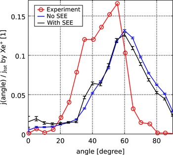
Angular ion current distribution with respect to the thruster exit at $r=0~\text{mm}$ , measured in experiment (Matyash et al. Reference Matyash, Kalentev, Schneider, Taccogna, Koch and Schirra2009) and simulated with SEE and without. Simulation results are given with statistic error bars.

3.1 Angular ion current distribution

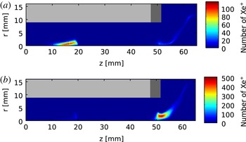
In figure 1, the calculated angular ion current distribution is given in blue. It shows contributions for all angles with a maximum current at $60^{\circ }$ . In the same figure a measured angular ion current distribution for the DM3a HEMP model is given in red. It shows two maximums at $35^{\circ }$ and $55^{\circ }$ , respectively. For a better understanding, the origin of the detected ions was diagnosed and analysed with respect to the angle. It indicates a correlation of the respective cusp, in which an ion is generated, and the angle into which it is emitted, as can be seen in figure 2, which shows the ionisation distribution for ions detected at $40^{\circ }$ and $60^{\circ }$ . While for angles between $30^{\circ }$ and $50^{\circ }$ , ions are mainly generated in the central cusp, for angles larger than $55^{\circ }$ the exit cusp apparently is the place of origin. Due to a low contribution of the ionisation in the central cusp, the second maximum around $40^{\circ }$ is not well accentuated. Therefore, the simulated ion angular current distribution can be seen as qualitatively matching the experimental data, shifted by $5^{\circ }$ towards higher angles.

Figure 2.

Ionisation distribution for ions detected at the diagnostic surface at $40\pm 2.5^{\circ }$ (a) and $60\pm 2.5^{\circ }$ (b). The dielectric channel wall is shown in light grey and the grounded pole piece is shown in dark grey.

Figure 3.

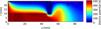
Potential of thruster channel and plume, given in $V$ . In magenta, the diagnostic surface for the ion angular distributions is given at the plume domain boundary. The small black box in the plume indicates the position of the electron source.

An important effect on the angular ion distribution is the potential drop in the plume, accelerating the ions towards different angles. In the simulation, it is also sensitive to the potential at the boundary of the simulation domain due to its limited size. In figure 3, the resulting potential is shown and in magenta, the diagnostic surface is indicated. The black rectangle at $r=20~\text{mm}$ and $z=75~\text{mm}$ indicates the position of the primary electron source with a source current of $I_{src,1}=0.3~\text{mA}$ . It represents the real neutraliser, which is located outside the computational domain. The position was chosen in order to provide sufficient starter electrons for the thruster channel. In experiments, the HEMP-T can operate even without the neutraliser because even a very small amount of free electrons are sufficient for successful start up. Corresponding ion and electrons distributions can be found in Duras et al. (Reference Duras, Schneider, Kalentev, Kemnitz, Matyash, Koch, Lüskow, Kahnfeld and Bandelow2016). For the boundary condition at the right-hand side of the domain $E_{z}=0$ is chosen. The potential at the left-hand side is fixed to the anode potential $U_{a}$ . At the upper boundary $\unicode[STIX]{x1D6F7}=0~\text{V}$ is used. This fixed potential can squeeze or stretch the potential solution in the radial direction, which results in shifted angular distributions. To prevent this, it is reasonable to use, for the area of the simulated plume, a similar aspect ratio as the vessel in which the experiments were taking place. What constitutes a sufficient domain size to reduce the influence of this defined potential boundary remains to be investigated.

An indirect influence on the potential is induced by the emission of secondary electrons from the vessel walls. These low energetic electrons are attracted by the anode potential and become magnetised by the magnetic field of the thruster acting as additional primary source of electrons. A study of different external electron sources and their positions showed strong influence of the magnetic field on the near-field plume (Duras et al. Reference Duras, Schneider, Kalentev, Kemnitz, Matyash, Koch, Lüskow, Kahnfeld and Bandelow2016). To represent the possible contributions of secondary electrons created by ions at the vessel walls, an electron source is placed close to the symmetry axis. This changes the potential distribution in the channel, while external electron sources at other places in the plume hardly influence the potential structure. The main reason for this is that the magnetic field, close to the symmetry axis, points directly into the thruster. At other radial positions the field lines are curved and electrons are trapped between a magnetic mirror movement, pushing them away from the thruster, and the potential drop forcing them towards the exit. Electrons emitted close to the symmetry axis have higher energies due to the direct guidance into the channel. This increases the probability of ionisation which expands the potential drop out of the thruster channel.

SEE at the aluminium vessel walls can act as an additional electron source. Secondary electrons created at the vessel walls by impinging ions fly towards the thruster. Rosenberg & Wehner (Reference Rosenberg and Wehner1962) measured sputter yields for singly charged ions impinging on aluminium which have been published for ion energies of 100, 200, 300 and 600 eV. With the help of an empirical fitting formula by Yamamura, Matsunami & Itoh (Reference Yamamura, Matsunami and Itoh1983), an emission coefficient of $\unicode[STIX]{x1D6FE}=0.6$ can be approximated for singly charged xenon ions impinging with an energy of 500 eV.

Approaching the thruster entrance such electrons experience an increasing magnetic field, which directs them mostly towards the axis. In the small simulation domain of this work, the electron influx from this process is parametrised as an additional surface source close to the axis. Electrons are injected at the right domain boundary close to the symmetry axis at $r\in (0;2~\text{mm})$ and $z\in (88~\text{mm};90~\text{mm})$ , with a directed drift velocity towards the thruster based on an energy of $100~\text{eV}$ corresponding to the potential at this location and a thermal broadening of the source distribution assuming a temperature of $0.45~\text{eV}$ . Of the total emitted ion current of $I_{tot}=142~\text{mA}$ , 10 % were chosen as an effective electron source close to the axis, representing SEE. This contribution is a factor of approximately 5 times higher than the primary electron source. This value was chosen because it induced a visible effect in the solution without affecting strongly the integral ion current.

The resulting angular current distribution with SEE can be seen in black in figure 1. It shows a higher ion contribution close to the symmetry axis ( $0^{\circ }$ ), which is the direct effect of the additional electron source in this region. At approximately $40^{\circ }$ the second ion beam becomes more pronounced, which is in qualitative agreement with the experimental data.

3.2 Angular ion energy distribution

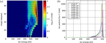
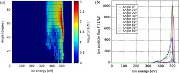
The simulated angular ion energy distribution calculated at the domain boundary is shown in figure 4. At the left-hand side the calculated ion flux is colour coded in logarithmic scale and the angle is defined with respect to the thruster exit at the symmetry axis. The right-hand side of figure 4 shows the same result in linear scale as line plots for nine angles. As expected, the maximum ion energy is 500 eV, given by the anode potential. The dominant contribution of ions originates from ions at approximately $60^{\circ }$ .

Figure 4.

Angular ion energy distribution at the domain boundary. (a) Contour plot of the ion particle flux $\unicode[STIX]{x1D6E4}_{i}$ in logarithmic scale as a function of angle and ion energy. (b)  $\unicode[STIX]{x1D6E4}_{i}$ in linear scale as a function of ion energy shown for nine angles.

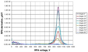
An experimentally measured energy distribution for the HEMP thruster model HEMPT 3050 is shown in figure 5 for nine different angles (Koch et al. Reference Koch, Schirra, Weis, Lazurenko, van Reijen, Haderspeck, Genovese, Holtmann, Schneider and Matyash2011). It is characterised by a maximum close to the anode potential $U_{a}=1000~\text{V}$ , with an opening angle of $20^{\circ }$ . While the simulated energy distribution shows a peak, smeared out to lower energies, the measured data show a Gaussian distribution around $U_{a}$ .

Figure 5.

Angular ion energy distribution for the HEMP thruster model HEMPT 3050, derived from RPA measurements. The applied thruster anode voltage was $U_{a}=1000~\text{V}$ (Koch et al. Reference Koch, Schirra, Weis, Lazurenko, van Reijen, Haderspeck, Genovese, Holtmann, Schneider and Matyash2011).

In the numerical diagnostic, the limited domain size causes differences between the simulated and measured ion energy distributions. In order to make the simulated ion distribution comparable to the experimentally measured one, a transfer function $g(f)$ , similar to the detector function in Reiter (Reference Reiter2009), is used to transfer information from the domain boundary to the detector position in the experiment

(3.1) $$\begin{eqnarray}g:f(\text{domain boundary})\mapsto f(\text{detector position}).\end{eqnarray}$$

Here $f$ stands for the angular ion energy distribution. This correction is used to represent effects which are not included in the current PIC simulation. One artefact caused by the limited domain size originates from the von Neumann boundary condition at the right-hand side of the domain. Ions reaching the diagnostic surface at this location have not yet reached the maximum kinetic energy of $U_{a}$ . For small angles, $0^{\circ }$ – $30^{\circ }$ , one can clearly see in figure 4 a reduction of the maximum energy, which is decreasing with the angle. At the detector position $1~\text{m}$ distant from the thruster exit, the potential will have relaxed to values close to ground potential and the additional acceleration by this potential drop has to be taken into account. Therefore, the transfer function $g(f)$ of the angular ion energy distribution corrects the ion energies of the detected ions by adding the additional potential at the domain boundary

(3.2) $$\begin{eqnarray}f(\text{detector position})=f(\text{domain boundary})+q_{i}\unicode[STIX]{x1D6F7}(\text{domain boundary}),\end{eqnarray}$$

with the ion charge $q_{i}$ . In figure 6, the corrected angular ion energy distribution can be seen. For angles ${<}35^{\circ }$ , the correction results in a shift to higher energies, so that for all angular bins the maximum energy corresponds to the anode potential $U_{a}$ . This improves the qualitative agreement between simulation and measured ion energy distribution (see figure 5).

Figure 6.

Mapped angular ion energy distribution to the location of the experimental detector position. (a) Contour plot of the ion particle flux $\unicode[STIX]{x1D6E4}_{i}$ in logarithmic scale as a function of angle and ion energy. (b)  $\unicode[STIX]{x1D6E4}_{i}$ in linear scale as a function of ion energy shown for nine angles.

Another discrepancy between experiment and simulation are the missing ion charge exchange (CX) collisions during the $1~\text{m}$ of flight within the plume. Within the PIC simulation, domain charge exchange collisions between ions and neutrals are fully included. While within the acceleration channel the mean free path of these collisions is smaller than the channel length, the decreasing neutral density increases this mean free path to approximately $1~\text{m}$ , which is larger than the simulated domain size. Therefore, CX collisions appearing between the domain boundary of the simulation and the position of the experimental measurement of the ion energy distribution are not represented within this simulation due to the latter’s limited domain size and require special corrections. This is visible in the missing low energetic part of the ion energy distribution of the simulation (figure 4), which clearly appear in the experimental measurements at about $0$ – $200~\text{eV}$ (figure 5). Here the idea of the transfer function, trying to map the information from the boundary of the simulated domain to the location of the experimental measurement, can be improved using a Monte Carlo post-processing procedure including CX collisions for a pre-defined neutral background gas density in the vessel.