1 Introduction
Current sheets are ubiquitous in space plasmas. They appear in magnetized collisionless plasmas as a result of the frozen-in law and the conservation of field line connectivity (Priest & Forbes Reference Priest and Forbes2000). An important consequence is the formation of tangential layers between plasmas of different origin and connectivity. The Earth’s magnetopause is certainly the most studied of these current sheets, separating the shocked solar wind plasma in the magnetosheath from the plasma of the Earth’s magnetosphere (Chou & Hau Reference Chou and Hau2012). Important dynamical processes can develop in the vicinity of tangential current sheets, and several can have system-wide consequences. For instance, magnetic reconnection occurring at the Earth’s magnetopause results in substantial transport of solar wind mass, momentum and energy into the magnetosphere, from which originates most of its internal activity. A prerequisite to understanding such processes is the correct modelling of the unperturbed tangential current sheet structures.
To understand the development of local microphysical processes, one can often make the assumption that current sheets are essentially one-dimensional (1-D) tangential layers, accounting only for the variations of physical quantities along the direction locally normal to the current sheet. As a result, in a steady state, the momentum equation across the layer can be written as a pressure balance:
 $nk_{B}T+B^{2}/2{\it\mu}_{0}=\text{const.}$
, where
 $n$
is the plasma density,
 $k_{B}$
the Boltzmann constant,
 $T$
the plasma temperature,
 $B$
the magnetic field and
 ${\it\mu}_{0}$
the vacuum permeability. If all 1-D steady-state tangential layers must satisfy this condition, it is however not a sufficient condition to be steady. Indeed, in collisionless media, the thickness of the boundaries can be of the order of the scale of the particle Larmor radius, meaning the system has to be described at the kinetic level. For instance, the magnetopause is approximately 1000 km wide, that is approximately 5 local Larmor ion radii, but can reach thicknesses of approximately 300 km (Dunlop & Balogh Reference Dunlop and Balogh2005). Then, not only the pressure balance should be satisfied, but the underlying particle distribution function
 $F(\boldsymbol{r},\boldsymbol{v})$
should be steady as well. In other words, any kinetic modelling starting from only a tangential pressure-balanced current sheet will not be steady and lead to a Larmor scale, self-consistent evolution of the current sheet (Fujimoto & Sydora Reference Fujimoto and Sydora2008; Pritchett Reference Pritchett2008; Aunai, Belmont & Smets Reference Aunai, Belmont and Smets2013).
Many works have been dedicated to finding kinetic equilibria, i.e. particle distribution functions such that
 $\partial F/\partial t=0$
. The most famous one is the Harris equilibrium model (Harris Reference Harris1962). It describes the distribution functions of both ions and electrons as drifting Maxwellians with constant drift velocities and temperatures across the layer. The Harris configuration is symmetric in density with a coplanar antisymmetric magnetic field without an electric field in the current sheet. As a result, the density tends to zero on both sides of the layer. This description is not suitable for most space tangential current sheets which can have different asymptotic properties, such as the Earth’s magnetopause. More general models have later been presented, possibly enabling asymmetric solutions (Alpers Reference Alpers1971; Channell Reference Channell1976; Lemaire & Burlaga Reference Lemaire and Burlaga1976; Roth, de Keyser & Kuznetsova Reference Roth, de Keyser and Kuznetsova1996; Mottez Reference Mottez2003), but some of their limitations have so far restricted their widespread use in theoretical and numerical modelling of current sheet processes such as magnetic reconnection. Indeed, in these models (hereafter said to follow the usual methods), the analytical form of the distribution function chosen for all species, and further assumptions used to solve the Vlasov–Maxwell system, fully constrain the fields and plasma profiles. As a result, the usual methodology of modellers, consisting of studying current sheet processes such as reconnection as a function of e.g. the magnetic field profile, is non-trivial and not possible unless the many parameters of the equilibrium theories are fine tuned in a rather non-intuitive way. Furthermore, starting from Jeans’s theorem, usual methods look for distribution functions which explicitly depend only on Hamiltonian invariants
 $k_{i}$
, which further constrain the solutions. Indeed, if any function of
 $k_{i}$
is a solution of Vlasov’s equation, the converse is not true. A solution of Vlasov’s equation can depend on other parameters and, in particular, it can depend on the position, which is more physically reasonable for an equilibrium in an inhomogeneous system. This explicit dependence on the position is allowed by the Vlasov equation in certain regions of the invariant space which depend on the magnetic topology. This concept of accessibility of the particles to the solution has only been used recently (Belmont, Aunai & Smets Reference Belmont, Aunai and Smets2012; Aunai et al.
Reference Aunai, Belmont and Smets2013) to find kinetic equilibria in asymmetric configurations (hereafter called the BAS model). The method is simply based on the fact that, at a position
 $y$
, particles do not access distributions located further than their Larmor radius. Imposing the distribution far from the layer, the local distribution can be determined step by step by moving along the normal direction across it. At a given step, the distribution in invariant space remains unchanged for all locations that correspond to particles already present in the previous step. On the contrary, all new locations can be filled by any prescribed function (analytical or not) of the invariants, using a model that can be chosen to satisfy macroscopic constraints such as being close to a given thermal pressure profile. Since there are no particles at infinite energy, distributions which are distant enough eventually become completely independent from one another, allowing asymmetric layers to exist. With a distribution function depending only on
 $k_{i}$
, in coplanar magnetic configurations, distributions have the same value for a given set
 $k_{i}$
, no matter how far they might be spatially. Usual methods then only lead to symmetric solutions in the absence of an electrostatic field. Such a field is therefore a necessary ingredient to obtain a stationary asymmetric layer with these methods, while it is not in the more general case considered in BAS. This apparently essential need for an electric field to sustain asymmetric solutions have been shown to be a purely artificial consequence of neglecting the explicit spatial dependence of the solutions allowed by the accessibility concept, which in itself allows us to build asymmetric solutions with vanishing electric fields. Considering real tangential layers, it then appears much more reasonable that they include both the normal electric field and the explicit dependence on the position. The BAS model has then recently been generalized to include the effect of a chosen electric field profile (Dorville et al.
Reference Dorville, Belmont, Aunai, Dargent and Rezeau2015).
The BAS model (Belmont et al.
Reference Belmont, Aunai and Smets2012) allows us to build equilibria with distribution functions
 $F(y,k_{i})$
that explicitly depend on the spatial position across the layer. To simplify the problem, this model describes the tangential current sheet with kinetic ions and fluid electrons. By fluid, we mean that only the electron density, bulk velocity and scalar pressure are accounted for in the model, which therefore is independent on the specific underlying electron distribution. This is a priori justified whenever the scale of the layer is of the order of the ion Larmor scale, which is much larger than that of the electrons. The BAS model was confirmed to be a steady state with a hybrid simulation (Aunai et al.
Reference Aunai, Belmont and Smets2013), which makes the same assumptions of kinetic ions and fluid electrons. However, one can legitimately wonder to what extent the steady state holds in fully kinetic models, where one needs to specify an electron distribution, not imposed by the model. In order to address this question, we perform fully kinetic simulations (i.e. with both kinetic ions and electrons) initialized with a solution found by the BAS model and study the evolution of the current sheet. Since this model does not impose the electron distribution, it will be arbitrarily chosen to follow a isotropic Maxwellian distribution, locally following the fluid moments imposed by the BAS model.
Considering that steady states have never been used in the literature as a starting point for kinetic simulations of asymmetric current sheet processes, we will extend this work to study the possible consequences of not controlling the internal profiles of the initial tangential current sheet and of the resulting unsteadiness (Fujimoto & Sydora Reference Fujimoto and Sydora2008; Aunai et al. Reference Aunai, Belmont and Smets2013) on the later physical processes developing in the layer. One of them, magnetic reconnection, is generally supposed to depend only on the upstream plasma properties and fields. This assumption is essential for interpreting spacecraft data but has never been tested. For that purpose, we compare 2-D fully kinetic simulations of magnetic reconnection with the same asymptotic plasma and field properties but different descriptions of the initial tangential current sheet. Their structure differs both microscopically, i.e. with or without a kinetic equilibrium, and macroscopically, i.e. with different profiles. We especially look for possible differences in the reconnection rate, as well as more detailed signatures of asymmetric reconnection such as the relative position of the magnetic neutral point (X point) and the electron flow stagnation point (Cassak & Shay Reference Cassak and Shay2007) or the predominance area of the different Ohm’s law terms (Hesse et al. Reference Hesse, Neukirch, Schindler, Kuznetsova and Zenitani2011, Reference Hesse, Aunai, Sibeck and Birn2014) discussed in the literature and searched for in Magnetospheric MultiScale (MMS) data.
The present paper is organized as follows: § 2 gives a quick overview of the numerical model and data normalization used for the simulations. In § 3, we demonstrate that the BAS model can be used to initialize fully kinetic particle-in-cell (PIC) simulations of magnetic reconnection with a steady-state ion-scale tangential current sheet. In § 4 we show simulations of magnetic reconnection with different initial particle distributions and compare the evolution of signatures mentioned above. Finally, § 5 contains a summary and outlook.
2 Numerical model and data normalization
In this paper, we present several fully kinetic simulations using a PIC code described in Hesse et al. (Reference Hesse, Schindler, Birn and Kuznetsova1999). All the simulations presented here share the same initial electromagnetic set-up, following the assumptions of the BAS model. The electric field
 $\boldsymbol{E}$
is supposed to be zero and all simulations share the same initial antisymmetric magnetic field
 $\boldsymbol{B}$
which is along the
 $x$
axis:
 $$\begin{eqnarray}\boldsymbol{B}=B_{x}(z)\boldsymbol{u}_{x}=B_{0}\tanh (z-z_{0})\boldsymbol{u}_{x},\end{eqnarray}$$
with
 $z_{0}=z_{max}/2$
the position of the current sheet and
 $\boldsymbol{u}_{x}$
the unit vector in the
 $x$
direction.
The data presented are normalized using ion-scale quantities. The magnetic field and density are normalized to arbitrary values
 $B_{0}$
and
 $n_{0}$
, respectively. The masses and charges are normalized to the proton mass
 $m_{p}$
and charge
 $e$
, time is normalized to the inverse of the proton gyrofrequency
 ${\it\omega}_{ci}^{-1}=m_{p}/eB_{0}$
and length to the proton inertial length
 ${\it\delta}_{i}=c/{\it\omega}_{pi}$
, where
 $c$
is the speed of light in a vacuum and
 ${\it\omega}_{pi}=\sqrt{n_{0}e^{2}/m_{p}{\it\epsilon}_{0}}$
is the proton plasma frequency.
3 Kinetic equilibrium in a full PIC simulation
The BAS model (Belmont et al. Reference Belmont, Aunai and Smets2012; Aunai et al. Reference Aunai, Belmont and Smets2013; Dorville et al. Reference Dorville, Belmont, Aunai, Dargent and Rezeau2015) was proven to provide a kinetic equilibrium explicitly dependent on the position in the layer. However, it assumes fluid electrons. We here study the impact of the kinetic nature of electrons on a kinetic equilibrium obtained from the BAS model. For this purpose, we run two 1-D fully kinetic simulations. One is initialized with the BAS model equilibrium, i.e. the proton distribution follows the kinetic solution. The other one has the same first moments but is not a kinetic equilibrium, i.e. protons are loaded, as usually done, in locally Maxwellian distributions. For both of them electrons are loaded with Maxwellian distribution functions. We first describe the initial set-up of both runs, then give an overview of their evolution at the ion scale, as has been previously done in hybrid simulations, and finally we inspect in more detail the behaviour of the electrons and their influence on the internal structure of the tangential current sheet.
3.1 Initial set-up
We perform two simulations of a 1-D asymmetric current layer named runs a and b. Run a is initialized with the BAS model. Run b is initialized with locally Maxwellian distribution functions for which the first two moments are those used in run a, i.e. the moments of the steady kinetic solution. The electron pressure for run b is considered isotropic and equal to the
 $zz$
term of the pressure tensor of run a. Run a is expected to be steady, as shown for a hybrid simulation, while run b is not (Aunai et al.
Reference Aunai, Belmont and Smets2013). As in the BAS model, we assume that the ratio of electron and ion currents is equal to
 $T_{e}/T_{i}$
, the electron to ion temperature ratio, which is chosen to be equal to 0.2 in the current work; a typical value for a magnetopause plasma. The mass ratio
 $m_{i}/m_{e}$
is 25 unless otherwise stated.
The simulation domain of runs a and b consists in a 1-D layer in the
 $z$
direction of size
 $z_{m}=36.4$
. There are
 $n_{z}=10\,000$
cells in this direction and at least 12 000 particles per cell. This large number of particles per cell is not required for the equilibrium to be steady but will decrease the noise level and allow for a more detailed analysis. The time step is
 $\text{d}t=10^{-3}$
and the total time of the simulation is
 $T=10$
, which is sufficient to study the validity of the BAS model and the effect of the lack of equilibrium in other models, which should manifest itself within the first few ion cyclotron periods. In the
 $z$
direction, the box is closed by reflecting boundary conditions, which are located far enough from the current sheet not to influence the result of the simulations.
Density profile of runs a and b.

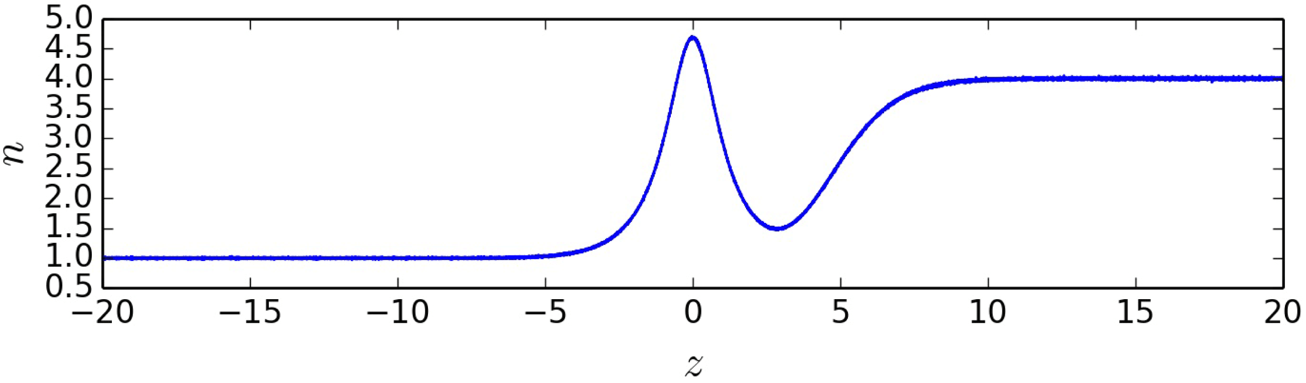
The density profile used to initialize runs a and b is showed in figure 1. It goes from 1 to 4. The density peak at the centre of the tangential current sheet is a generic feature of equilibria calculated with the BAS model, mainly resulting from neglecting the magnetic field rotation and the normal electric field. These assumptions have been relaxed in a recent generalization of the BAS model (Dorville et al.
Reference Dorville, Belmont, Aunai, Dargent and Rezeau2015), but the use of this new model is left for future work. The BAS model provides for the ions an analytical distribution function
 $F(E,P_{y},z)$
depending on the position
 $z$
and invariants of motion, i.e.
 $E$
the energy and
 $P_{y}$
the generalized momentum along
 $y$
axis (Belmont et al.
Reference Belmont, Aunai and Smets2012). However, we have to load particles such that
 $(z,\boldsymbol{v})=(z,v_{x},v_{y},v_{z})$
. To do this, we use the rejection method, as recently done to initialize hybrid simulations (Aunai et al.
Reference Aunai, Belmont and Smets2013). For a given position, we take a random velocity
 $\boldsymbol{v}$
, we deduce
 $(E,P_{y})$
and reject or not the created particle, depending on the value of a random number drawn uniformly between
 $0$
and
 $\max (F)$
. We then repeat the process until we meet the desired density at that location. As the BAS model does not impose any distribution for electrons, we use the first three moments
 $(n_{i},\boldsymbol{V}_{i},\boldsymbol{P}_{i})$
of the BAS equilibrium, where the ions only are kinetic, and deduce
 $(n_{e},\boldsymbol{V}_{e},\boldsymbol{P}_{e})$
for the electrons. We obtain the density assuming
 $n_{e}=n_{i}$
, the current density
 $\boldsymbol{V}_{e}=-(T_{e}/T_{i})~\boldsymbol{V}_{i}$
and the scalar pressure
 $P_{e}=(T_{e}/T_{i})~P_{izz}$
. Knowing
 $(n_{e},\boldsymbol{V}_{e},\boldsymbol{P}_{e})$
, we load electrons within Maxwellian distributions, as done for run
 $\boldsymbol{b}$
.
Total pressure for different
 $t$
. (a) Total pressure for run a (equilibrium). (b) Total pressure for run b (non-equilibrium).

3.2 BAS equilibrium: test and comparison
In steady state, the sum of thermal and magnetic pressures through the layer has to be constant. We plot in figure 2 this total pressure for run a and run b at different times. The tangential current sheet is localized at
 $z=0$
. In both cases the initial total pressure is constant. In figure 2(a), one can see that for run a, the total pressure remains equal to its initial value throughout the current sheet, to within the noise level. However, figure 2(b) reveals that this is not the case for run b. In this run, the total pressure starts oscillating as soon as
 $t=1$
within the current sheet and those oscillations are observed to propagate away with time approximately at the Alfvén velocity. The amplitude of these oscillations reaches here 10 % of the initial total pressure, but it can be larger depending on the initial profile of the layer (Aunai et al.
Reference Aunai, Belmont and Smets2013). Whether those fluctuations are to be considered important or not will depend on the final application.
Our main point here is that run a confirms that even within a fully kinetic simulation, the BAS model can be successfully used to initialize steady-state tangential current sheets, despite providing a distribution function for the ions alone. On the other hand, run b confirms that not using kinetic solutions for the ions, but only its first moments with Maxwellian distributions, results in unsteadiness of the tangential current sheet (Aunai et al. Reference Aunai, Belmont and Smets2013). This unsteadiness occurs within the first ion cyclotron period and results from local finite Larmor radius effects.
3.3 Influence of locally Maxwellian electron distributions
We have just seen that not knowing the kinetic steady state for electrons does not affect the global equilibrium with regards to the total pressure. We will show now that they are however responsible for small-scale unsteadiness. This unsteadiness mostly affects the current density of the electrons.
Current density of electrons
 $Jy_{e}$
for different times in run a. The black thick curve is the theoretical
 $Jy_{e}$
used to initialize the simulation at
 $t=0$
. The vertical dashed lines represent the boundary of bounce widths. The red lines show the ion bounce width and the purple ones the electron bounce width.

Figure 3 displays, for different times, the electron current density. The black thick line is the initial current density imposed by the BAS model. The vertical dashed lines mark the boundary of ion and electron bounce widths, i.e. where the local thermal Larmor radius is equal to the distance to the centre of the layer (Hesse et al.
Reference Hesse, Neukirch, Schindler, Kuznetsova and Zenitani2011). One can notice that the current density is steady almost everywhere, but that a structure can be observed to slowly grow in the centre of the layer. It must therefore be concluded that not knowing a steady distribution for the electrons does not affect the pressure balance but has an effect on the electron moments at electron scales. Indeed, the unsteadiness stays confined within the electron bounce width, i.e. this is an electron-scale effect which does not affect the ion scales. To confirm this, we ran another simulation, a*, with exactly the same parameters as run a except for the mass ratio, which was
 $m_{i}/m_{e}=100$
. The results (not shown here) reveal that the unsteadiness stays confined within the new (and reduced) electron bounce width, which confirms its electron kinetic origin. In simulations using a realistic mass ratio, the scale of such effects, as well as its amplitude compared to the noise level, would make it completely negligible. This result confirms that neglecting the kinetic behaviour of electrons, as is done in the BAS model, is a reasonable assumption in building kinetic equilibria for asymmetric ion scale tangential current sheets. Let us furthermore add that, in the case of the tangential magnetopause, for instance, the current sheet is often even wider than the ion scales.
4 Asymmetric magnetic reconnection: sensitivity to the initial current sheet structure
Simulations of asymmetric magnetic reconnection usually start from pressure balanced, locally Maxwellian tangential current sheets as an initial condition (Pritchett Reference Pritchett2008; Hesse et al. Reference Hesse, Aunai, Sibeck and Birn2014). As we have already seen, such a configuration is fundamentally unsteady in collisionless models and results in waves and relaxation of the current sheet internal structure. Many authors have noticed these effects (Fujimoto & Sydora Reference Fujimoto and Sydora2008; Aunai et al. Reference Aunai, Belmont and Smets2013) and wondered to what extent not using a kinetic equilibrium as an initial state matters. When no equilibrium is used, one has to assume that the microphysics processes under investigation do not remember the initial conditions and only depend on the properties of the inflowing asymptotic plasmas. We present here the results of simulations of asymmetric reconnection sharing the same asymptotic plasma properties but different initial structures of the tangential current sheet, among which are layers initialized with a kinetic equilibrium or locally Maxwellian plasmas. Doing so will allow us to assert the robustness of some previously discussed reconnection features seen in simulations upon which the interpretation of in situ measurements, e.g. from the MMS mission, may be based. Among the usual methods available in the literature, we continue to use the BAS model as a kinetic equilibrium since it allows us to choose the magnetic field profile exactly and the first part of this study has shown it can be successfully used to initialize steady-state ion-scale current sheets.
4.1 Initial set-up
We present three simulations of 2-D asymmetric magnetic reconnection, respectively named runs A, B and C. Run A is initialized with a BAS model equilibrium for ions and locally Maxwellian distribution functions for the electrons. Run B is initialized with locally Maxwellian distribution functions for both ions and electrons but shares the first two moments of run A, i.e. the moments of the steady kinetic solution, and the pressure is chosen to be isotropic and equal to the component
 $zz$
of the pressure tensor of run A. Run C is also initialized with Maxwellian distribution functions but with arbitrary moments satisfying the pressure balance condition (here with a monotonic density profile). In all three runs, the plasma and fields are uniform along the
 $x$
direction. Their magnetic field is given by (2.1) and the density ratio between asymptotic plasmas is 2. We assume that the ratio of electron and ion currents is equal to
 $T_{e}/T_{i}$
, the electron to ion temperature ratio, chosen equal to
 $0.2$
in the current work. The mass ratio
 $m_{i}/m_{e}$
is 25.
The simulation domain of runs A, B and C consists of a 2-D layer in the
 $(x,z)$
plane of size
 $(x_{m},z_{m})=(69,45)$
. There are
 $n_{x}=3000$
cells in the
 $x$
direction,
 $n_{z}=1500$
cells in the
 $z$
direction and at least 200 particles per cell. The time step is
 $\text{d}t=10^{-3}$
and the total time of the simulation is
 $T=200$
, which is sufficient to reach a steady state of asymmetric reconnection in all simulations. In the
 $z$
direction, the box is closed by reflecting boundary conditions. These boundary conditions are far enough from the current sheet to not influence the results until the final time of the simulation. The domain is periodic in the
 $x$
direction.
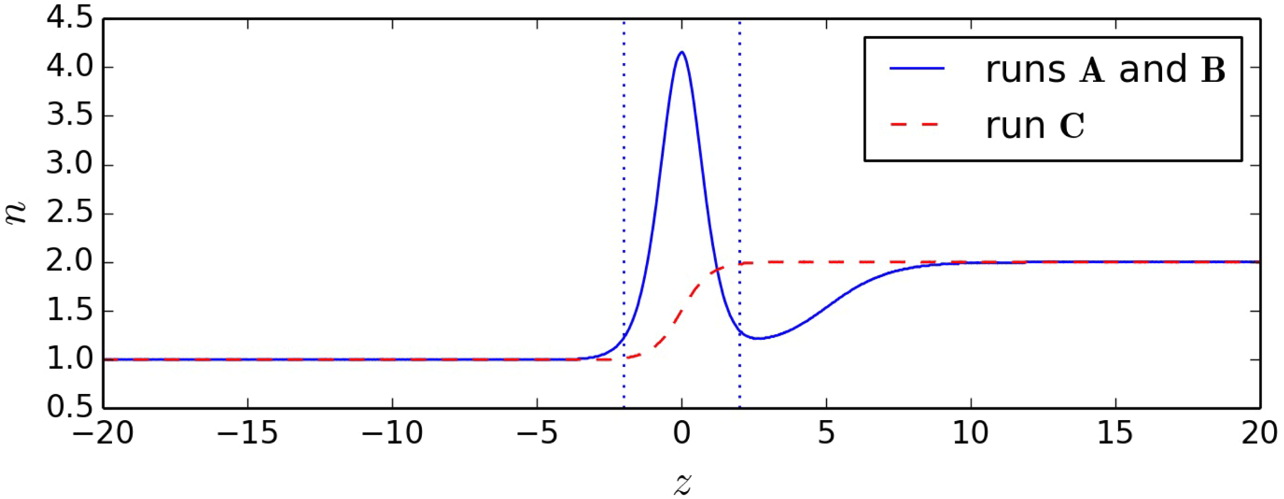
The density profiles used to initialize runs A, B and C are showed in figure 4. Density goes from 1 to 2. To compare with simulation set-ups usually chosen in current sheet models, the density for run C is chosen to be monotonic with asymptotic values equal to those of runs A and B. The density profile of run C is given by
 $n(z)=n_{1}+0.5(n_{2}-n_{1})(\tanh (z-z_{0})+1)$
, where
 $n_{1}=1$
,
 $n_{2}=2$
and
 $z_{0}=z_{m}/2$
. The initial magnetic field
 $\boldsymbol{B}_{0}$
is antisymmetric (see (2.1)) and the temperature is calculated in order to satisfy pressure balance. Initial parameters such as the ratio of upstream densities differ from those of § 3 mainly for computational reasons. In the three runs, we impose a perturbation
 $\boldsymbol{B}_{1}$
on the initial magnetic field
 $\boldsymbol{B}_{0}$
in order to trigger magnetic reconnection:
 $$\begin{eqnarray}\displaystyle & \displaystyle \boldsymbol{B}_{1}=B_{1x}(x,z)\boldsymbol{u}_{x}+B_{1z}(x,z)\boldsymbol{u}_{z} & \displaystyle\end{eqnarray}$$
 $$\begin{eqnarray}\displaystyle & \displaystyle B_{1x}(x,z)=-2{\it\delta}b\frac{z-z_{0}}{{\it\sigma}}\exp -\frac{(x-x_{0})^{2}+(z-z_{0})^{2}}{{\it\sigma}^{2}} & \displaystyle\end{eqnarray}$$
 $$\begin{eqnarray}\displaystyle & \displaystyle B_{1z}(x,z)=2{\it\delta}b\frac{x-x_{0}}{{\it\sigma}}\exp -\frac{(x-x_{0})^{2}+(z-z_{0})^{2}}{{\it\sigma}^{2}}, & \displaystyle\end{eqnarray}$$
 $z_{0}=z_{m}/2$
,
 $x_{0}=x_{m}/2$
,
 ${\it\delta}b=0.3$
and
 ${\it\sigma}=3$
.
Density profiles in the
 $z$
direction of runs A, B and C. The dotted lines delimit the area where the density profile of runs A and B is approximately symmetric.

4.2 Current sheet relaxation
Initialized with an equilibrium from the BAS model, run A is steady. Runs B and C are not steady and the internal structure of their tangential current sheets is self-consistently reconfigured within the first ion cyclotron periods. Figure 5 represents the different terms of the electron force balance across the layer during these early times, far from the reconnection site that eventually develops. Although the electric field is initially zero in all runs, only run A keeps this characteristic. A small imbalance between the pressure and the ideal terms appears in run B while run C reveals a large reconfiguration associated with a strong bipolar electric field. This last feature in run C is consistent with previous findings (Pritchett Reference Pritchett2008; Aunai et al. Reference Aunai, Belmont and Smets2013).
 $z$
axis component of Ohm’s law terms through the tangential current layer far from the reconnection site. (a) Run A. (b) Run B. (c) Run C. Curves are obtained by averaging 100 points in time for times between
 $t=3$
and
 $4~{\it\omega}_{ci}^{-1}$
.

4.3 Reconnection rate
Figure 6(a,b) offer us an overview of the three simulations through the time evolution of the reconnection rate. The first thing to notice is the similarity of all three rates in the late quasi-steady period. This demonstrates that the intrinsic structure of the initial tangential current sheet does not have a major impact on the global evolution. In particular, runs A and B are remarkably similar. The unsteadiness observed in run B (figure 5) and the subsequent waves emitted by the current sheet have no noticeable effect on the later nonlinear phase of the reconnection process. Run C however, is noticeably different from the others, due to its different macroscopic initialization. Figure 4 shows how the density profiles differ between runs (A, B) and C. The non-monotonic density profile of the first two runs results in a slightly more complex evolution than what occurs in the latter.
(a,b) Reconnection rate versus time of runs A and B (a,c) and run C (b,d). (c,d) Density versus time measured
 ${\it\delta}_{i}$
above and below X point for the run A (a,c) and the run C (b,d).

The influence of the density profile on the reconnection rate can be understood if one looks at figure 6. In the case of runs A and B, the reconnection rate suddenly increases as the plasma from the central dense layer is ejected and replaced by a plasma of much lower, quasi-symmetrical density. At
 $t\approx 50$
however, the incoming plasma becomes increasingly asymmetric, which lowers the reconnection rate. This is when the plasma processed by reconnection starts to increase towards that typical of asymptotic plasmas. At
 $t\approx 130$
, this asymmetry in the density becomes steady and the rate settles into a steady state as well. Around
 $t\approx 180$
, the domain boundaries in the upstream and downstream directions start to impact the dynamics and lower the reconnection rate. In the case of run C, the density profile is monotonic and the reconnection process is asymmetric right from the early phase, as can be seen on figure 6(c,d). The reconnection rate nonetheless seems to reach a maximum around
 ${\approx}0.4$
before decreasing to a quasi-steady value similar to that of runs A and B, i.e. at
 ${\approx}0.28$
. This overshoot, at
 $t\approx 30$
frequently occurs in simulations and depends on the initial current sheet thickness (Shay, Drake & Swisdak Reference Shay, Drake and Swisdak2007). It must not be confused with the peak of runs A and B, mostly resulting from the non-monotonic density profile.
Interestingly, one can also note that in run C the reconnection rate fluctuates quite a lot more than in the other two simulations. This is very probably a consequence of being initially quite far from a kinetic equilibrium. The large unsteadiness results in waves throughout the system which perturb the layer and favour the formation of large plasmoids. Figure 7 shows a plasmoid in run C at
 $t=111$
. This plasmoid appears at a slightly earlier time and is clearly associated with the sudden increase of the reconnection rate at this time (see figure 6). A similar plasmoid is observed approximately
 $t=140$
, and is associated with the second fluctuation in the reconnection rate on figure 6.
Ion density in 2-D for run C at
 $t=111~{\it\omega}_{ci}^{-1}$
. The picture is centred on the reconnection site. Black lines represent magnetic field lines.

4.4 Evolution of magnetic reconnection signatures
The interpretation of in situ measurements is, and will continue to be, largely based on comparison to simulation data, especially in the context of the NASA/MMS mission, where detailed measurements of the critical ion and electron decoupling regions are expected. In this section, we investigate some key features of the reconnection region and how they may vary as a result of different initializations for identical asymptotic plasma properties.
4.4.1 X line motion
In all runs, the X line location is not steady. Let us first investigate its motion. Figure 8 shows the position of the X point in the box for the three runs. One can note the motion of the X point in the
 $x$
direction in (a). Such a drift is usually seen in guide field simulations and is associated with diamagnetic effects (Swisdak et al.
Reference Swisdak, Rogers, Drake and Shay2003; Pritchett & Mozer Reference Pritchett and Mozer2009). Recent asymmetric simulations without a guide field have, however, revealed some motion in that direction (Malakit et al.
Reference Malakit, Shay, Cassak and Bard2010). In our case, a careful investigation of the processes occurring nearby the X point reveal that the changes in direction or speed are always associated with the appearance of plasmoids. Whenever an island appears on one side of the dominant X line, it temporarily prevents a proper plasma outflow from developing in that direction and results in the X line drifting in the other direction. As can be seen in figure 8, all three runs start to drift at
 $t\approx 60$
. The reason is that just before this time, the reconnection rate of all runs has significantly decreased. This drop in the rate is associated with an increased aspect ratio of the reconnection current sheet, which therefore becomes increasingly sensitive to plasmoid instabilities (Daughton, Scudder & Karimabadi Reference Daughton, Scudder and Karimabadi2006). Some of them are large enough to affect the reconnection rate, such as those of run C at
 $t\approx 100$
and
 $140$
(see figure 6). It is interesting to note that these two plasmoids have inverse effects on the reconnection rate despite both are moving to the left side of the X line and are of approximately equal size. As soon as one plasmoid forms, its motion on whatever side breaks the left–right macroscopic symmetry, which in turn influences the motion of subsequent plasmoids. This memory can last for tens of ion cyclotron periods. For instance, the plasmoid at
 $t\approx 140$
in run C appears in a region with a substantial left–right asymmetry caused by the plasmoid produced at
 $t\approx 100$
.
In figure 8(b), we can see that the X point is slowly drifting in the
 $z$
direction towards the low density side. The drift in the
 $z$
direction is related to the density asymmetry across the reconnecting current sheet. In the case of runs A and B, it starts at
 $t\approx 30$
, which is, as one can see in figure 6, approximately the time at which the asymmetry of the two inflowing plasmas starts to become non-negligible. Run C appears to drift right from the start of the simulation. This can be caused by the difference in the initial density profile. This drift would be unnoticeable in observations. For example, for
 $B=40~\text{nT}$
and
 $n=5~\text{m}^{-3}$
(typical values at the magnetopause), the drift velocity is
 ${\approx}1~\text{km}~\text{s}^{-1}$
, which is negligible compared to typical magnetopause speeds (De Keyser et al.
Reference De Keyser, Dunlop, Owen, Sonnerup, Haaland, Vaivads, Paschmann, Lundin and Rezeau2005).
Position of the X point in
 $x$
and
 $z$
directions versus time.

4.4.2 Electron flow stagnation point
A recent discovery in the context of asymmetric reconnection is that, contrary to what occurs in symmetric configurations, the X line and the ion and electron flow stagnation points are not collocated (Cassak & Shay Reference Cassak and Shay2007, Reference Cassak and Shay2009). As a result, there is a net flow across the X line and the off-diagonal components of the pressure tensor do not necessarily balance the reconnection electric field at the X line, while they do so at the stagnation point (Hesse et al.
Reference Hesse, Aunai, Sibeck and Birn2014). Figure 9 shows, for run A, the position of the electron flow stagnation point (S point) in the
 $x$
and
 $z$
directions, together with the position of the X point. Contrary to the X line, the location of the S point depends on the reference frame one chooses, since it is defined by
 $\boldsymbol{v}=\mathbf{0}$
in this frame. We represent this position in the simulation reference frame and in the X line reference frame. The latter is obtained by calculating the time derivative of the X line position on which a Gaussian filter has been applied to avoid large fluctuations. The inherent noise in PIC simulation makes the detection of the S point difficult. Our method consists in detecting the minimum of the in-plane velocity squared
 $v_{ex}^{2}+v_{ez}^{2}$
smoothed with a 2-D Gaussian filter in the proximity of the X point. A visual inspection (figure 10
c) confirms the detection is consistent with what appears to be the S point, and the fluctuation level of that detection is of the same order as the one for the X point, i.e. smaller than the relative distance between X and S points. As expected, figure 9 reveals that the S point is not collocated with the X point in the
 $z$
direction. At early times in the simulation, one may notice that the
 $z$
location of the S point oscillates but on average is equal to that of the X point, however at
 $t\approx 20{-}30$
, it starts to systematically be found below the X line. Again, this time is associated with the incoming, increasingly asymmetric plasmas, as seen in figure 6. The S point is, after that time, always on the low density side of the X line, which is consistent with recent findings (Cassak & Shay Reference Cassak and Shay2007). It is interesting to note that the motion of the X line towards the low density region results in a shorter distance to the S point in the X line frame, but is not sufficient in this case to reverse the relative position. Comparing the measured relative distance S–X in the X line frame with recently derived scaling laws does not reveal a good agreement, which may be related to the insufficient steadiness of the process, an electron mass effect or to more fundamental assumptions used in the model regarding, for instance, the way the mass and energy fluxes are partitioned within the decoupling region (Aunai, Belmont & Smets Reference Aunai, Belmont and Smets2011).
In the absence of a guide field, one may expect the S and X point to be at the same
 $x$
position. This is very well satisfied until
 $t\approx 60$
. After that time, the lower reconnection rate leads to the formation of plasmoids, resulting, as explained earlier, in the motion of the X line. They create a local asymmetry in the outflow direction and decouple the S point from the X point (Murphy, Sovinec & Cassak Reference Murphy, Sovinec and Cassak2010). Interestingly, we see in figure 9 that the S point is following the X line with a small time delay. The tension force driving reconnection originates from the X line, but it takes some time for the electron flow to adjust to this change. Overall, similar patterns are found in runs B and C, but for the latter the fluctuation level makes such a careful analysis more difficult.
Position of X point versus time in
 $x$
and
 $z$
directions, electron flow stagnation point in the box reference frame and electron flow stagnation point in the X point reference frame for run A.

(a,b) Ohm’s law terms through the current sheet at the X point (a) and the electron flow stagnation point (b) for run A. The vertical dashed line show, respectively, the X point and S point position in
 $z$
. These curves, and the following ones, are an average over 400 points in time between
 $t=150$
and
 $t=154$
. (c) Ohm’s law pressure term in 2-D for run A. The mean X point is shown by a blue cross and the mean S point by a green point. Their standard deviation in time is represented by an ellipse of the same colour. Arrows illustrate the in-plane velocity. (d) Same as the central panel but for the electron inertial term. Dashed black lines are the electron bounce width boundaries. Solid grey lines represent magnetic field lines.

4.4.3 Structure of the electron decoupling region
A key issue is to understand which mechanism breaks the field line connectivity in magnetic reconnection. This question can, to some extent, be addressed by investigating which term balances the reconnection electric field at the X line. It has been accepted for a long time that in space plasmas, whether reconnection occurs in antiparallel or guide field configurations, the non-gyrotropic part of the electron pressure tensor dominates. Recent findings however have shown that this is limited to the special case of symmetric reconnection, and that the electron inertia dominates at the X line for asymmetric configurations (Hesse et al. Reference Hesse, Aunai, Sibeck and Birn2014). The pressure tensor term, somehow related to dissipation, remains dominant at the flow stagnation point. Since there should be some continuity between symmetric and asymmetric results, it is interesting to understand to what extent previous findings depend on the degree of asymmetry of the system. For instance, we have observed that our asymmetry is sufficient to impact the reconnection rate, to make the X line drift and to separate the X point from the S point. We now proceed to looking at the structure of the terms balancing the reconnection electric field.
Figure 10(a,b) show the different terms of the electron Ohm’s law in a cut along
 $z$
at the
 $x$
position of the S and X points, during the asymmetric steady state of run A. Figure 10(c,d) show the 2-D structure of the electron pressure tensor term and electron inertia term, respectively. On both of these panels, we have indicated the position of the X and S points at that time. The random motion of the X and S points is small compared to their relative distance, as shown in figure 10 with uncertainty ellipses. Although the asymmetry is sufficient to make the X and S points non-collocated and drifting, it is clear from figure 10 that the electron decoupling region looks much like previous results of symmetric reconnection. In particular, the pressure tensor term dominates both at the X and S points, and the electron inertia is rather symmetric around the midplane. Looking very carefully at the position of the vertical dashed grey line, one can see that the pressure term is exactly equal to the reconnection electric field at the S point, whereas at the X point, the inertia term has a small contribution. The fact that only the pressure term can contribute to the reconnection electric field at the electron flow stagnation point, and both the pressure and inertia term can contribute at the X point, is consistent with recent findings (Hesse et al.
Reference Hesse, Aunai, Sibeck and Birn2014). We can see that the electron inertia term is positive only in two bands which match the bounce width boundaries (dashed black lines in figure 10
d). Electrons bouncing around the midplane appear, in the
 $z$
direction, as counterstreaming beams (Aunai et al.
Reference Aunai, Belmont and Smets2013) which effectively decrease the bulk velocity of the incoming plasma and result in an important inertia term.
Ohm’s law terms and electric field, i.e. their sum, through the reconnecting current layer for runs A, B and C along the
 $y$
axis. The curves are the average over 400 points in time between
 $t=150$
and
 $t=154$
. The vertical dashed line is the position of the mean X point for run A.

Figure 11 now compares these different terms for runs A, B and C at the position of the X point once magnetic reconnection reaches a steady state. As shown previously, terms depending on the magnetic field vanish at the X point (
 $z\approx -0.7$
), where the electric field is mainly supported by the pressure term. One can see that all the signatures are remarkably robust and do not depend on the initial structure of the tangential current layer, whether it is a kinetic equilibrium, locally Maxwellian or even with arbitrary pressure-balanced profiles.
5 Summary and discussion
Being ubiquitous and the locus of many dynamical phenomena, the modelling of tangential current sheets is a major topic in space plasma physics. Nowadays, however, there are very few models describing steady asymmetric current layers at kinetic scales. The BAS model (Belmont et al. Reference Belmont, Aunai and Smets2012) is one of them, enabling us to build a kinetic equilibrium for ions with an easy control over asymptotic properties of the plasma and electromagnetic field profiles. However, this model tends to produce a spike at the layer in the density profile. Furthermore, it assumes fluid electrons and thus does not provide distribution functions for them. A legitimate question was to understand to what extent this assumption prevents the use of the BAS model in fully kinetic models, i.e. to what extent the kinetic nature of the electrons matters. In this paper, we have tested equilibria found by the BAS model in fully kinetic simulations, using locally Maxwellian distribution functions for the electrons. We have proved that, even without a steady distribution function for the electrons, the tangential current sheet remains very well pressure balanced, while ignoring the kinetic solution results in large initial fluctuations and reconfiguration of the moments and fields. Unsteadiness resulting from the electron initialization stays confined within the electron bounce width. This result provides support to the BAS model hypothesis of fluid electrons and provides an adequate kinetic equilibrium to initialize fully or hybrid kinetic simulations with asymmetric current sheets.
In a second step, we used the BAS model to investigate the sensitivity of magnetic reconnection simulations to initial unsteadiness. We have compared two simulations with same profiles initialized with and without a kinetic equilibrium. We did another run, initialized with arbitrary pressure-balanced profiles, as usually done in the community. All the runs share the same properties for the asymptotic upstream plasmas. We carefully studied key features of interest for future interpretation of MMS data in the electron decoupling region. In particular, we found that our degree of asymmetry is sufficient to separate the electron flow stagnation point from the X line and to impact the reconnection rate. In the absence of a guide field, the position of the X line and the reconnection rate can also be occasionally perturbed by the formation of plasmoids. We notice that the slowing or increasing of the reconnection rate due to a plasmoid does not seem to be related either to its size or to the direction in which it moves. The asymmetry is, however, not strong enough to significantly alter the qualitative structure of the terms of the Ohm’s law in that region compared to symmetric models. A detailed analysis reveals that the electron inertia term contributes very little at the X line, whereas the pressure term is the sole contributor at the electron flow stagnation point. With a stronger asymmetry, the system will continuously evolve towards a more extreme case where the pressure tensor may eventually be negligible at the X line (Hesse et al. Reference Hesse, Aunai, Sibeck and Birn2014). A comparison between all runs indicates that all signatures are very robust and do not depend on the initial internal state of the current layer, at least for the upstream parameters we have used.
The BAS model for asymmetric equilibrium is now proven to be usable in fully kinetic simulations. A recent extension (Dorville et al. Reference Dorville, Belmont, Aunai, Dargent and Rezeau2015) has been proposed to generalize the tangential current sheets to rotating magnetic fields and non-zero normal electric fields. These extensions can help better control the density variation. In particular, an appropriate electric field profile can decrease and even suppress the density spike. In these non-coplanar magnetic configurations, the effects associated with kinetic electrons will be even more negligible. When started in the nonlinear phase, reconnection has been shown in this paper to depend only on asymptotic properties of the upstream plasmas, which provides more confidence in comparisons of simulations with observations based on upstream plasma parameters. This confirms that having a kinetic equilibrium or not is not crucial when studying this phase of the process. Having an initial steady state mostly facilitates the analysis because it drastically reduces fluctuations from the initial condition and prevents the formation of large plasmoids.
It is clear that the observed fluctuations associated with non-steady initialization do not allow for the study of collisionless instabilities. Future work should use asymmetric equilibria to study current sheet instabilities such as the tearing mode or Kelvin–Helmholtz modes. At this phase, the nature of the kinetic equilibrium is not only expected to be important, but not having a steady state precludes the study of instabilities in the first place. Such a study however requires a low-noise model such as used in the delta-f or Vlasov codes because PIC simulations are inherently too noisy. This will be the goal of a forthcoming study.
Acknowledgement
This is a pleasure to thank L. Rezeau for enlightening discussions regarding this work. The authors acknowledge the ANR for funding the project MON-ANR (ANR-13-PDOC-0027) supporting this research. This work was granted access to the HPC resources of CINES and IDRIS under the allocation i2015047231. Some simulations were also performed on CALMIP. We would like to especially thanks IDRIS staff for their help with regarding computational devices.