1. Introduction
The importance of the mechanisms whereby turbulent boundary-layer (TBL) flows undergo separation and subsequent reattachment has long been recognized in aerodynamics. While several decades of experimental, theoretical and computationally-based research have both clarified and categorized several salient features of the TBL separation/reattachment process, a general understanding of separated flow remains elusive; see Simpson (Reference Simpson1989) for a review. At the same time, the rapid growth of computational resources has enabled some accurate predictions of separation/reattachment flows using direct numerical simulation (DNS) at low Reynolds numbers (Na & Moin Reference Na and Moin1998). At larger Reynolds numbers, typical of real engineering applications, advances in the numerical simulation of separated flows past bodies with complex geometry have been made using wall-modelled large-eddy simulation (LES) or detached-eddy simulation (DES) strategies (Spalart Reference Spalart2009).
For flow past either a streamlined or bluff-body, such as an airfoil or cylinder, respectively, critical factors that may induce or affect either incipient or actual separation of a TBL are the wall curvature in one or two directions, or the presence of an adverse pressure gradient (APG) or some combination of these. A somewhat simpler flow that nonetheless offers a natural setting for the study of the fundamental structure of separation is the flat-plate TBL with an imposed APG. The attraction here is the absence of curvature but the presence of the reasonably well understood, canonical TBL prior to separation. Further, there exists several well documented studies of separation/reattachment of the flat-plate TBL that can provide validation cases for simulations over a range of Reynolds numbers. Presently, we develop and apply a wall model suitable for the LES of separated flow that provides direct calculation of the surface skin friction vector and allows detailed comparison between wall-modelled LES and experimental results for separation and reattachment of a flat-plate TBL at low to moderate Reynolds numbers.
The systematic study of separation in flat-plate TBL flow perhaps began in the 1970s. Perry & Fairlie (Reference Perry and Fairlie1975) investigated a nominally two-dimensional (in the mean) turbulent separation bubble in a wind tunnel with a tailored diverging–converging roof system designed to produce first, a region of adverse pressure gradient flow that induced separation of the TBL on the flat-plate floor below, followed by a steep favourable pressure gradient that forced shear-layer reattachment. In order to minimize the unwanted effects of boundary-layer separation on the upper wall on the separation bubble flow below, their roof system consisted of two disconnected and separate diverging and converging parts, staggered and overlapped so that the gap separating the parts swallowed the (possibly separating) boundary layer generated on the diverging part. They investigated two cases with different pressure gradient profiles, the first of which generated a closed separation bubble, while the second produced incipient but not actual separation. They also developed a simple separation model which utilized an inviscid region of uniform vorticity to represent the separation bubble and which proved capable of reproducing some average properties of the experimental data.
Later, Simpson and co-workers systematically studied separating turbulent boundary layers, beginning with separation induced by an airfoil-type pressure gradient (Simpson, Strickland & Barr Reference Simpson, Strickland and Barr1977) and subsequently using a series of experiments that investigated velocity profile scalings up to separation, together with some higher-order moments (Simpson, Chew & Shivaprasad Reference Simpson, Chew and Shivaprasad1981a ,Reference Simpson, Chew and Shivaprasad b ), and also a scaling for backflow velocity inside the bubble (Simpson Reference Simpson1983). Patrick (Reference Patrick1987) employed the Perry & Fairlie (Reference Perry and Fairlie1975) two-roof strategy to produce a large-scale separation bubble with an extremely strong imposed pressure gradient, showing that separated flow generally follows Simpson’s velocity profile scaling. Patrick also found interesting reattachment behaviour which is quite unsteady and somewhat similar to that observed in separation from a backward-facing step. Recently, Lögdberg, Angele & Alfredsson (Reference Lögdberg, Angele and Alfredsson2008) investigated three separation flows each with a mild pressure gradient. They argued that their mean-velocity defect profiles showed reasonable similarity for separated regions. A study of separation in an axisymmetric turbulent boundary layer (Alving & Fernholz Reference Alving and Fernholz1996) has also improved our general understanding of separation induced by an adverse pressure gradient.
DNS of turbulent boundary-layer separation was performed by Spalart & Coleman (Reference Spalart and Coleman1997), who noted that a prescribed pressure gradient along the boundary layer could be generated by imposing a tailored normal velocity distribution on the upper boundary of a rectangular computational domain. Using DNS, Na & Moin (Reference Na and Moin1998) give a detailed discussion of the flow characteristics near separation and reattachment, finding that the mean velocity profile before separation deviates from both a linear law and logarithmic form, and that the reattachment zone is unsteady. Skote & Henningson (Reference Skote and Henningson2002) argue that the flow near separation can be analysed using two velocity scales obtained from a boundary-layer equation. Na & Moin (Reference Na and Moin1998) and Skote & Henningson (Reference Skote and Henningson2002) are both at
 $Re_{{\it\theta}}\approx 300$
where
 $Re_{{\it\theta}}=U_{\infty }{\it\theta}/{\it\nu}$
is the Reynolds number based on the momentum boundary-layer thickness
 ${\it\theta}$
,
 $U_{\infty }$
is the free-stream velocity and
 ${\it\nu}$
is the kinetic viscosity of the flow. Recently, Abe et al. (Reference Abe, Mizobuchi, Matsuo and Spalart2012) extended the case of Na & Moin (Reference Na and Moin1998) to
 $Re_{{\it\theta}}=986$
, which is still well below Perry & Fairlie (Reference Perry and Fairlie1975) (
 $Re_{{\it\theta}}\approx 2000$
) and Patrick (Reference Patrick1987) (
 $Re_{{\it\theta}}=11\,000$
).
LES has proven a useful tool for the numerical simulation of turbulent free-shear and wall-bounded flows at large Reynolds numbers. In LES, the flow on turbulent length scales, at or larger than the local grid resolution, are simulated directly within the algorithmic discretization scheme, while the range of scales below a cutoff length scale, usually proportional to the grid size, is modelled. LES of wall-bounded turbulent flows generally fall into two categories; wall-resolved and wall-modelled. In wall-resolved LES, for example Abe et al. (Reference Abe, Mizobuchi, Matsuo and Spalart2012), the simulation can be viewed as hybrid LES–DNS, with the near-wall either fully or nearly resolved. While useful, wall-resolved LES is presently limited to flows where
 $\log (Re_{{\it\tau}})$
is not large, where
 $Re_{{\it\tau}}\equiv u_{{\it\tau}}\,{\it\delta}/{\it\nu}$
, with
 ${\it\delta}$
an outer length scale and
 $u_{{\it\tau}}=\sqrt{|{\it\tau}_{w}|/{\it\rho}}$
the friction velocity.
In order to achieve larger
 $\log (Re_{{\it\tau}})$
, while eliminating the need to resolve near-wall motions, wall-modelled LES generally introduces a subgrid-scale (SGS) model at the wall that recognizes both near-wall anisotropy of the unresolved small-scale turbulence and also the no-slip condition, while communicating the wall-normal flux of energy and momentum to the outer flow; see Piomelli & Balaras (Reference Piomelli and Balaras2002) for a review. Two major issues for wall-modelled LES are first, capturing Reynolds-number effects that can be weak for attached flows and second, the adequate modelling of flow separation. Useful approaches to the latter have included hybrid methods that implement a Reynolds-averaged Navier–Stokes (RANS) model very near the wall, merged with conventional LES away from solid surfaces, for example Constantinescu & Squires (Reference Constantinescu and Squires2004), and the use of a slip boundary condition based on use of a differential filter as described by Bose & Moin (Reference Bose and Moin2014).
The essence of the present wall model, henceforth referred to as the virtual-wall model, is the application of a near-wall integration strategy to obtain an ordinary differential equation (ODE), at each wall point describing the time variation of an instantaneous, filtered or window-averaged wall skin-friction velocity. This ODE is then numerically evolved to provide boundary condition information for LES in the bulk of the flow. The model also proposes use of a plane parallel to, but displaced above, the physical wall. A Dirichlet velocity boundary condition is applied on this plane, which is, for the outer-flow LES, considered as a virtual wall. The offset of the virtual wall is set to be proportional to the mesh size, which ensures the convergence of fine mesh LES to DNS. To provide the velocity boundary condition, Chung & Pullin (Reference Chung and Pullin2009) developed a log-like relationship obtained from the stretched-vortex subgrid model under an assumption of linear scaling of the wall-parallel vortex scale with distance from the wall. The virtual-wall model has been applied and validated for LES of both smooth- and rough-wall channel flow (Saito, Pullin & Inoue Reference Saito, Pullin and Inoue2012; Saito & Pullin Reference Saito and Pullin2014) and to fully-developed turbulent boundary-layer flow for both zero pressure gradient (Inoue & Pullin Reference Inoue and Pullin2011; Inoue et al. Reference Inoue, Mathis, Marusic and Pullin2012) and attached-flow APG cases (Inoue et al. Reference Inoue, Pullin, Harun and Marusic2013). As an alternative to the sub-virtual wall modelling leading to a log-variation for the slip velocity, Cheng & Samtaney (Reference Cheng and Samtaney2014) used a power-law relation for the virtual-wall slip velocity. For the zero-pressure gradient boundary layer they found little effect on the calculated outer-flow properties.
Chung & Pullin (Reference Chung and Pullin2009) made the strong assumption that the wall-shear stress lies in the direction of the outer free-stream flow. While this may be reasonable for wall-attached boundary layers, it cannot describe a general flow near a wall where, on the wall itself, the wall-shear stress is a surface vector field whose field lines are everywhere orthogonal to the vorticity at the wall, and in general will not be approximately parallel to the driving, outer free-stream flow. The purpose of the present work is first, to extend our LES capability, with calculation of the wall shear stress, to separated flow at moderately large Reynolds numbers, and second, to apply this capability to the study of boundary-layer separation/reattachment in the form of a separation bubble flow. The virtual-wall model is presently extended to two wall-parallel dimensions. It will be shown that this treatment of the wall-slip boundary condition allows local backflow near the virtual wall with respect to an outer free stream, and permits accurate LES modelling of separation/reattachment flows.
In the following section, the development of the two-dimensional wall model is described in § 2. In § 3 the present numerical LES strategy is outlined including discussion of the virtual-wall boundary condition. This is followed by a description of the LES for two cases of flow in a turbulent separation bubble. Section 4 contains an account of the present strategy for simulation of the experimental conditions. This section also describes a comparison with the medium Reynolds number, mild pressure gradient experiments of Perry & Fairlie (Reference Perry and Fairlie1975). The LES of the higher-Reynolds number, sharper pressure gradient case of Patrick (Reference Patrick1987) is discussed in § 5. Further parametric studies and the prospects for more detailed simulations are discussed in § 6.
2. Physical model
In implementing wall-modelled LES, both a SGS model for the outer flow and a wall model are required. The latter is essentially an SGS model designed specifically to recognize the special character of near-wall flow, including the no-slip boundary condition. We employ the stretched vortex SGS model introduced by Misra & Pullin (Reference Misra and Pullin1997), and further developed by Voelkl, Pullin & Chan (Reference Voelkl, Pullin and Chan2000) and Chung & Pullin (Reference Chung and Pullin2009). This last-cited version is used presently for the outer flow without modification. In this section, we first summarize the stretched vortex SGS model to provide a closure for LES simulation. Then an extended wall model is derived.
2.1. Stretched vortex SGS model
In LES, the velocity components
 $u_{i}$
and pressure
 $p$
can be decomposed as a resolved part and an unresolved part:
 $u_{i}=\tilde{u_{i}}+u_{i}^{\prime }$
,
 $p=\tilde{p}+p^{\prime }$
. After applying a filter with scale
 ${\it\Delta}_{c}$
, the filtered Navier–Stokes (N–S) equations can be written as
 $$\begin{eqnarray}\displaystyle {\displaystyle \frac{\partial \widetilde{u_{i}}}{\partial t}}+{\displaystyle \frac{\partial \widetilde{u_{i}}\widetilde{u_{j}}}{\partial x_{j}}}=-{\displaystyle \frac{\partial \tilde{p}}{\partial x_{i}}}+{\it\nu}{\displaystyle \frac{\partial ^{2}\widetilde{u_{i}}}{\partial x_{j}^{2}}}-{\displaystyle \frac{\partial \unicode[STIX]{x1D61B}_{ij}}{\partial x_{j}}},\quad {\displaystyle \frac{\partial \widetilde{u_{i}}}{\partial x_{i}}}=0, & & \displaystyle\end{eqnarray}$$
with the subgrid stress (SGS) tensor
 $\unicode[STIX]{x1D61B}_{ij}\equiv \widetilde{u_{i}u_{j}}-\widetilde{u_{i}}\widetilde{u_{j}}$
. The subscript
 $i$
or
 $j$
presently denotes three components
 $x$
,
 $y$
and
 $z$
, corresponding to the streamwise, spanwise and wall-normal directions, respectively. The three velocity components are also written as
 $u$
,
 $v$
and
 $w$
.
The stretched-vortex SGS model owes its genesis to the stretched-spiral vortex model by Lundgren (Reference Lundgren1982). The model assumes that in each computational cell, the subgrid motion is dominated by a vortex with direction
 $\boldsymbol{e}^{v}$
, modelled by a delta-function probability density function. The SGS tensor is modelled as Chung & Pullin (Reference Chung and Pullin2009):
 $$\begin{eqnarray}\unicode[STIX]{x1D61B}_{ij}=({\it\delta}_{ij}-e_{i}^{v}e_{j}^{v})K,\quad K=\int _{k_{c}}^{\infty }E(k)\,\text{d}k=\mathscr{K}_{0}^{\prime }{\it\Gamma}[-1/3,{\it\kappa}_{c}^{2}]/2\end{eqnarray}$$
with
 $k_{c}={\rm\pi}/{\it\Delta}_{c}$
the cutoff wavenumber,
 $k$
the wavenumber, and
 $E(k)$
the energy spectrum. In the integration above, the Lundgren vortex model is used, with
 $\mathscr{K}_{0}^{\prime }=\mathscr{K}_{0}{\it\epsilon}^{2/3}{\it\lambda}_{{\it\nu}}^{2/3}$
,
 ${\it\Gamma}$
is an incomplete Gamma function with
 ${\it\kappa}_{c}=k_{c}{\it\lambda}_{{\it\nu}}$
,
 ${\it\lambda}_{{\it\nu}}=(2{\it\nu}/(3|\tilde{a}|))^{1/2}$
,
 $\tilde{a}=e_{i}^{v}e_{j}^{v}\widetilde{\unicode[STIX]{x1D61A}}_{ij}$
is the stretching along the subgrid vortex and
 $\widetilde{\unicode[STIX]{x1D61A}}_{ij}=(\partial \widetilde{u}_{i}/\partial x_{j}+\partial \widetilde{u}_{j}/\partial x_{i})/2$
is the resolved strain-rate tensor.
By using a matching procedure, the constant
 $\mathscr{K}_{0}^{\prime }$
can be found as
 $\mathscr{K}_{0}^{\prime }=\langle F_{2}\rangle /\langle Q({\it\kappa}_{c},d)\rangle$
. Here
 $\langle ~\rangle$
denotes the local average and is computed technically from a set of 26 neighbouring points, and
 $F_{2}$
is the local second-order velocity structure function calculated from the resolved velocities. The quantity
 $$\begin{eqnarray}Q({\it\kappa}_{c},d)=4\,\int _{0}^{{\it\kappa}_{c}}{\it\kappa}^{-5/3}\text{e}^{-{\it\kappa}^{2}}[1-J_{0}(({\it\kappa}/{\it\kappa}_{c})\,{\rm\pi}d)]\,\text{d}{\it\kappa},\end{eqnarray}$$
is calculated using an efficient asymptotic approximation with
 $d=r/{\it\Delta}_{c}$
and
 $r$
is the distance from neighbour point to the vortex axis (Chung & Pullin Reference Chung and Pullin2009).
The SGS model discussed above is utilized in the main body of the flow. For modelling near-wall flow, Chung & Pullin (Reference Chung and Pullin2009) developed an extended SGS model based on the idea that the convection of both the passive scalars and the axial velocity inside cylindrical SGS vortices can be analysed within a two-dimensional, three-component flow framework. This leads to an additional term added to the original SGS model
 $$\begin{eqnarray}\unicode[STIX]{x1D61B}_{ij}=K({\it\delta}_{ij}-e_{i}^{v}e_{j}^{v})-K_{s}\left[e_{j}^{v}e_{k}^{v}{\displaystyle \frac{\partial \tilde{u_{k}}}{\partial x_{l}}}({\it\delta}_{li}-e_{l}^{v}e_{i}^{v})+e_{i}^{v}e_{k}^{v}{\displaystyle \frac{\partial \tilde{u_{k}}}{\partial x_{l}}}({\it\delta}_{lj}-e_{l}^{v}e_{j}^{v})\right]\end{eqnarray}$$
with
 $K_{s}={\it\gamma}{\it\Delta}_{c}K^{1/2}/2$
and
 ${\it\gamma}$
a ‘mixing’ constant. This SGS model was used in the virtual-wall model to obtain the wall-normal flux of wall-parallel momentum in the near wall region.
2.2. Wall model
Chung & Pullin (Reference Chung and Pullin2009) argue that the dominant parameter for near wall-modelling is
 $u_{{\it\tau}}$
. In order to calculate
 $u_{{\it\tau}}$
without resolving the fine scales near the wall, they introduce wall-normal averaging of the wall-parallel, streamwise (outer flow) momentum equation combined with local inner scaling used to treat the time-dependence of the filtered, wall-parallel velocity. This latter assumption requires no specific form for the wall-normal variation of this velocity. This results in an ODE describing the local wall-normal velocity gradient
 ${\it\eta}_{0}=\partial \tilde{u} /\partial z|_{w}$
or equivalently
 $u_{{\it\tau}}^{2}\equiv {\it\nu}\,{\it\eta}_{0}$
, at each wall point with coefficients and source terms that, with a few-point approximation to certain wall-normal integrals, can be determined dynamically from the outer LES at the first few grid points away from the wall. Combined with a log-based description of the slip velocity at a virtual wall at a distance
 $h_{0}$
(to be defined later) from the actual wall that is a small fraction of the first wall-normal grid location, this provides closure.
Following this approach, we begin with the Navier–Stokes equations and apply two filters:
 $$\begin{eqnarray}\displaystyle & \displaystyle \tilde{{\it\phi}}(x,y,z,t)=\int \int {\it\phi}(x^{\prime },y^{\prime },z,t)G(x-x^{\prime };{\it\Delta}_{f})G(y-y^{\prime },{\it\Delta}_{f})\,\text{d}x^{\prime }\,\text{d}y^{\prime }, & \displaystyle\end{eqnarray}$$
 $$\begin{eqnarray}\displaystyle & \displaystyle \langle {\it\phi}\rangle ={\displaystyle \frac{1}{h}}\int _{0}^{h}\tilde{{\it\phi}}(x,y,z,t)\,\text{d}z, & \displaystyle\end{eqnarray}$$
 $xy$
-plane) quantity
 $\tilde{{\it\phi}}$
and (2.6) defines a wall-normal (
 $z$
) or top-hat filter
 $\langle {\it\phi}\rangle$
. For the wall-parallel velocity components these are presently
 $\tilde{u}$
and
 $\tilde{v}$
and
 $\langle u\rangle$
and
 $\langle v\rangle$
, respectively. We remark that presently, the wall-parallel filtering is strictly formal.
After applying the wall-parallel filter to both the streamwise and spanwise momentum equations, neglecting lateral diffusion, we obtain
 $$\begin{eqnarray}\left.\begin{array}{@{}c@{}}\displaystyle {\displaystyle \frac{\partial \tilde{u} }{\partial t}}+{\displaystyle \frac{\partial \widetilde{u\phantom{\!~\!}u}}{\partial x}}+{\displaystyle \frac{\partial \widetilde{uv}}{\partial y}}+{\displaystyle \frac{\partial \widetilde{uw}}{\partial z}}=-{\displaystyle \frac{\partial \tilde{p}}{\partial x}}+{\it\nu}{\displaystyle \frac{\partial ^{2}\tilde{u} }{\partial z^{2}}},\\ \displaystyle {\displaystyle \frac{\partial \tilde{v}}{\partial t}}+{\displaystyle \frac{\partial \widetilde{vu}}{\partial x}}+{\displaystyle \frac{\partial \widetilde{vv}}{\partial y}}+{\displaystyle \frac{\partial \widetilde{vw}}{\partial z}}=-{\displaystyle \frac{\partial \tilde{p}}{\partial y}}+{\it\nu}{\displaystyle \frac{\partial ^{2}\tilde{v}}{\partial z^{2}}}.\end{array}\right\}\end{eqnarray}$$
2.2.1. Inner scaling assumption and ODE of
 ${\it\eta}_{0}$

The virtual-wall model adopts an inner scaling assumption, which states that very near the wall, the SGS, instantaneous wall-filtered, wall-parallel velocity scales locally with the time-dependent
 $u_{{\it\tau}}(x,y,t)$
and
 ${\it\nu}$
. This is a widely-accepted standard for mean-velocity profiles, sufficiently close to the wall, in either steady or statistically stationary, wall-bounded flows such as laminar boundary layer, turbulent channel flow, the TBL and also the APG TBL. While its strict accuracy for the fluctuating, near-wall filtered velocity profile is unknown, it was shown to work well in LES determination of the mean wall-friction velocity for both the ZPG and APG TBLs (Chung & Pullin Reference Chung and Pullin2009; Inoue & Pullin Reference Inoue and Pullin2011).
For the purposes of wall modelling in a virtual-wall region
 $h_{0}>z\geqslant 0$
, where
 $h_{0}$
is much smaller than the thickness of the wall layer, we presently assume that the magnitude of the resultant velocity in the wall-parallel plane
 $\tilde{q}=(\tilde{u} ^{2}+\tilde{v}^{2})^{1/2}$
, follows inner scaling. We then have
 $$\begin{eqnarray}{\displaystyle \frac{\tilde{q}}{u_{{\it\tau}}}}=F(z^{+}),\quad z^{+}\equiv {\displaystyle \frac{z}{l^{+}}}={\displaystyle \frac{zu_{{\it\tau}}}{{\it\nu}}},\end{eqnarray}$$
where
 $F(z^{+})$
is unknown, together with
 $$\begin{eqnarray}{\it\eta}_{0}\equiv \left.{\displaystyle \frac{\partial \tilde{q}}{\partial z}}\right|_{0},\quad u_{{\it\tau}}^{2}={\it\nu}{\it\eta}_{0},\quad {\displaystyle \frac{\partial u_{{\it\tau}}}{\partial {\it\eta}_{0}}}={\displaystyle \frac{{\it\nu}}{2u_{{\it\tau}}}}={\displaystyle \frac{1}{2}}\left({\displaystyle \frac{{\it\nu}}{{\it\eta}_{0}}}\right)^{1/2},\quad {\displaystyle \frac{\partial z^{+}}{\partial {\it\eta}_{0}}}={\displaystyle \frac{z^{+}}{2{\it\eta}_{0}}}.\end{eqnarray}$$
Applying the wall-normal filter to the time derivative of
 $\tilde{q}$
then gives
 $$\begin{eqnarray}{\displaystyle \frac{\partial \langle q\rangle }{\partial t}}={\displaystyle \frac{\tilde{q}|_{h}}{2{\it\eta}_{0}}}{\displaystyle \frac{\partial {\it\eta}_{0}}{\partial t}},\quad \tilde{q}|_{h}\equiv u_{{\it\tau}}F(h^{+}),\end{eqnarray}$$
where we note that, in obtaining (2.10) wall-normal integrals containing
 $F(z^{+})$
in the integrand cancel. If
 $\tilde{q}|_{h}$
in (2.10) is identified as the resolved-scale fluid speed at the first grid point off the wall, then here, the specific form of
 $F(z^{+})$
is not required. From the definition of
 $\tilde{q}$
, we obtain
 $$\begin{eqnarray}\displaystyle {\displaystyle \frac{\partial \langle q\rangle }{\partial t}} & = & \displaystyle {\displaystyle \frac{1}{h}}\int _{0}^{h}{\displaystyle \frac{1}{(\tilde{u} ^{2}+\tilde{v}^{2})^{1/2}}}\left(\tilde{u} {\displaystyle \frac{\partial \tilde{u} }{\partial t}}+\tilde{v}{\displaystyle \frac{\partial \tilde{v}}{\partial t}}\right)\,\text{d}z.\end{eqnarray}$$
Then combining (2.11) with the momentum equations (2.7), and using (2.10) for the unsteady term, we have an equation for
 ${\it\eta}_{0}$
as
 $$\begin{eqnarray}\displaystyle {\displaystyle \frac{\tilde{q}|_{h}}{2{\it\eta}_{0}}}{\displaystyle \frac{\partial {\it\eta}_{0}}{\partial t}} & = & \displaystyle {\displaystyle \frac{1}{h}}\int _{0}^{h}\left[-{\displaystyle \frac{1}{\tilde{q}}}\left(\tilde{u} {\displaystyle \frac{\partial \widetilde{u\phantom{\!~\!}u}}{\partial x}}+\tilde{u} {\displaystyle \frac{\partial \widetilde{uv}}{\partial y}}+\tilde{u} {\displaystyle \frac{\partial \widetilde{uw}}{\partial z}}+\tilde{v}{\displaystyle \frac{\partial \widetilde{vu}}{\partial x}}+\tilde{v}{\displaystyle \frac{\partial \widetilde{vv}}{\partial y}}+\tilde{v}{\displaystyle \frac{\partial \widetilde{vw}}{\partial z}}\right)\right.\nonumber\\ \displaystyle & & \displaystyle \left.+\,{\displaystyle \frac{1}{\tilde{q}}}\left(-\tilde{u} {\displaystyle \frac{\partial \tilde{p}}{\partial x}}+{\it\nu}\tilde{u} {\displaystyle \frac{\partial ^{2}\tilde{u} }{\partial z^{2}}}-\tilde{v}{\displaystyle \frac{\partial \tilde{p}}{\partial y}}+{\it\nu}\tilde{v}{\displaystyle \frac{\partial ^{2}\tilde{v}}{\partial z^{2}}}\right)\right]\text{d}z.\end{eqnarray}$$
2.2.2. Treatment of near-wall region
The integration on the right-hand side of (2.12) can be further simplified. Using integration by parts, for the viscous term, one can obtain
 $$\begin{eqnarray}-\int _{0}^{h}{\displaystyle \frac{1}{\tilde{q}}}\left(\tilde{u} {\displaystyle \frac{\partial ^{2}\tilde{u} }{\partial z^{2}}}+\tilde{v}{\displaystyle \frac{\partial ^{2}\tilde{v}}{\partial z^{2}}}\right)\text{d}z=\left.{\displaystyle \frac{\partial \tilde{q}}{\partial z}}\right|_{h}-{\it\eta}_{0}-\int _{0}^{h}\left[{\displaystyle \frac{1}{\tilde{q}}}\left(\left({\displaystyle \frac{\partial \tilde{u} }{\partial z}}\right)^{2}+\left({\displaystyle \frac{\partial \tilde{v}}{\partial z}}\right)^{2}-\left({\displaystyle \frac{\partial \tilde{q}}{\partial z}}\right)^{2}\right)\right]\text{d}z.\end{eqnarray}$$
For the purposes of modelling we make the approximation that, within the first grid cell
 $0\leqslant z\leqslant h$
, the angle
 ${\it\theta}\equiv \arccos (\tilde{u} /\tilde{q})$
is constant. The last term in the above equation is then zero. Also, terms such as
 $\tilde{u} /\tilde{q}$
and
 $\tilde{v}/\tilde{q}$
will then be constant in the wall-normal direction and integration over them is straightforward. Using these results, performing all integrations on integrands expressed as
 $\partial ../\partial z$
and applying exact no-slip boundary conditions at
 $z=0$
, (2.12) can then be written as
 $$\begin{eqnarray}\displaystyle & & \displaystyle {\displaystyle \frac{\tilde{q}|_{h}^{2}}{2{\it\eta}_{0}}}{\displaystyle \frac{\text{d}{\it\eta}_{0}}{\text{d}t}}+\left.\left(\tilde{u} {\displaystyle \frac{\partial \langle uu\rangle }{\partial x}}+\tilde{u} {\displaystyle \frac{\partial \langle uv\rangle }{\partial y}}+\tilde{v}{\displaystyle \frac{\partial \langle vu\rangle }{\partial x}}+\tilde{v}{\displaystyle \frac{\partial \langle vv\rangle }{\partial y}}+\tilde{u} {\displaystyle \frac{\partial \langle p\rangle }{\partial x}}+\tilde{v}{\displaystyle \frac{\partial \langle p\rangle }{\partial y}}\right)\right|_{h}\nonumber\\ \displaystyle & & \displaystyle \quad +\,{\displaystyle \frac{1}{h}}\left.\left(\tilde{u} \,\widetilde{uw}+\tilde{v}\,\widetilde{vw}\right)\right|_{h}-{\displaystyle \frac{{\it\nu}\tilde{q}|_{h}}{h}}\left(\left.{\displaystyle \frac{\partial \tilde{q}}{\partial z}}\right|_{h}-{\it\eta}_{0}\right)=0.\end{eqnarray}$$
Each
 $\langle \cdots \rangle$
or tilde term in above equation can be estimated by resolved-scale quantities near, or at, the first grid point
 $z=h$
above the wall. For example, nonlinear terms are approximated by LES resolved-scale values at
 $z=h$
as
 $$\begin{eqnarray}{\displaystyle \frac{\partial \langle uu\rangle }{\partial x}}\approx {\displaystyle \frac{\partial \widetilde{u\phantom{\!~\!}u}|_{h}}{\partial x}}={\displaystyle \frac{\partial \tilde{u} |_{h}\tilde{u} |_{h}}{\partial x}}+{\displaystyle \frac{\partial T_{xx}|_{h}}{\partial x}},\end{eqnarray}$$
with similar approximations for other terms. The wall-normal integrated pressure
 $\langle p\rangle$
is also approximated as
 $\tilde{p}|_{h}$
. Equation (2.14) can then be interpreted as a nonlinear ODE for
 ${\it\eta}_{0}$
.
Once
 ${\it\eta}_{0}(x,y,t)$
is known and
 ${\it\theta}$
is estimated as
 ${\it\theta}={\it\theta}_{0}$
, the angle of the shear stress at the wall is known, then the local wall-shear stress components can be calculated as
 $$\begin{eqnarray}{\displaystyle \frac{{\it\tau}_{w,x}}{{\it\rho}}}={\it\nu}\,{\it\eta}_{0}\,\cos {\it\theta}_{0},\quad {\displaystyle \frac{{\it\tau}_{w,y}}{{\it\rho}}}={\it\nu}\,{\it\eta}_{0}\,\sin {\it\theta}_{0}.\end{eqnarray}$$
where
 $\boldsymbol{{\it\tau}}_{w}\equiv ({\it\tau}_{w,x},{\it\tau}_{w,y})$
is the LES representation of the surface stress vector. Since the wall-parallel momentum equations have been (formally) filtered in two wall-parallel directions, then the present estimate of
 $\boldsymbol{{\it\tau}_{w}}$
should be interpreted as a wall-parallel filtered and not a point-wise version of this quantity. We presently investigate two models for the estimation of
 ${\it\theta}_{0}$
as follows:
-
(1)
${\it\theta}_{0}={\it\theta}_{h}\equiv \arccos (\tilde{u} |_{h}/\tilde{q}|_{h})$
, namely the flow angle at
$z=h=h_{0}+{\rm\Delta}z/2$
. This is extremely simple and is referred to as model I; -
(2) obtain an independent equation for
${\it\theta}_{0}$
using similar arguments to those leading to (2.14) for
${\it\eta}_{0}$
. This is done in appendix A and is referred to as model II.




The ODE (2.14) is independent of the possible presence of local backflow at
 $z=h$
, with respect to the outer free stream. Note that, by construction, we expect that
 ${\it\eta}_{0}>0$
except possibly at a finite number of critical points of the surface stress vector field. In principle, these can occur when
 $\tilde{q}|_{h}=0$
which means the appearance of an actual wall-parallel stagnation point at the first wall-normal grid cell. In real turbulent separated flow at large Reynolds number, the area measure of critical points of
 $\boldsymbol{{\it\tau}_{w}}$
is unknown but is expected to be zero. Likewise, the grid-set measure of stagnation points in the wall parallel direction (that is
 $\tilde{q}|_{h}=0$
at a grid point) is also expected to be zero, and in fact none has been encountered in the present LES. This is discussed further in appendix B. Presently we demonstrate that (2.14) works well for flow that is considered to be separated. In passing, we remark that there appears to be no precise definition of separation for spatially three-dimensional flow.
2.2.3. Slip wall boundary conditions
The wall model is completed with a slip velocity specified at a raised virtual plane at
 $z=h_{0},h_{0}<h$
. The slip velocity may represent a back flow with respect to the outer free stream. The slip velocity used presently is defined by
 $$\begin{eqnarray}\displaystyle \left.\tilde{q}\right|_{h_{0}}=\left\{\begin{array}{@{}ll@{}}\left\{\begin{array}{@{}ll@{}}u_{{\it\tau}}\left({\displaystyle \frac{1}{\mathscr{K}_{1}}}\log \left({\displaystyle \frac{h_{0}^{+}}{h_{{\it\nu}}^{+}}}\right)+h_{{\it\nu}}^{+}\right),\quad & h_{0}^{+}>h_{{\it\nu}}^{+},\\ u_{{\it\tau}}h_{0}^{+},\quad & h_{0}^{+}<h_{{\it\nu}}^{+},\end{array}\right.\quad & {\it\tau}_{w,x}>0,\\ \quad u_{{\it\tau}}\,h_{0}^{+},\quad & {\it\tau}_{w,x}\leqslant 0,\end{array}\right. & & \displaystyle\end{eqnarray}$$
where
 $h_{0}^{+}\equiv h_{0}\,u_{{\it\tau}}/{\it\nu}$
and
 $h_{{\it\nu}}^{+}$
is a parameter to be discussed. For
 ${\it\tau}_{w,x}>0$
the above is essentially a log/linear version of the slip velocity used by Chung & Pullin (Reference Chung and Pullin2009) and derived from the stretched-vortex SGS model in the near-wall region, with dynamic calculation of the Kármán-like parameter
 $\mathscr{K}_{1}$
. This is used everywhere except where
 $h_{0}^{+}<h_{{\it\nu}}^{+}$
where a simple linear relationship is used. In (2.17),
 $z^{+}=h_{{\it\nu}}^{+}$
is a standard division of the viscous sublayer and the log layer. Presently,
 $h_{{\it\nu}}^{+}=11$
is used which is an empirical parameter of the present model. The condition
 ${\it\tau}_{w,x}<0$
, which is the present version of the more general condition
 ${\bf\tau}_{w}\boldsymbol{\cdot }\boldsymbol{U}_{\infty }<0$
, is interpreted presently as the wall-model indication of local back flow. In this case it is considered that a state of ordered boundary-layer-like flow has broken down. While it cannot be ruled out that a sufficiently ordered back flow could produce an equilibrium wall layer with its own log-like behaviour, we presently use a simple linear relationship consistent with local inner scaling, namely
 $\tilde{u} ^{+}=z^{+}$
. We remark that, sufficiently close to the wall, the latter relation is always valid except at critical points of the surface stress field.
In Chung & Pullin (Reference Chung and Pullin2009) for channel flow,
 $h_{0}/{\rm\Delta}z=0.18$
remains fixed with respect to the computational grid and the sensitivity to changes was documented. Their collated mesh arrangement results in
 $h=h_{0}+{\rm\Delta}z$
, but this relation is not required by the wall model. Inoue & Pullin (Reference Inoue and Pullin2011) extended the model to turbulent boundary-layer flow. Their staggered mesh strategy changes the relation to
 $h=h_{0}+{\rm\Delta}z/2$
while retaining
 $h_{0}/{\rm\Delta}z=0.18$
. Their verification shows good convergence and reasonable agreement for the near-wall physical variables. Presently we follow Inoue & Pullin (Reference Inoue and Pullin2011).
Since
 $h_{0}$
is fixed,
 $h_{0}^{+}$
can be calculated locally using
 $u_{{\it\tau}}=\sqrt{{\it\nu}{\it\eta}_{0}}$
where
 ${\it\eta}_{0}>0$
is known from the solution of (2.14). In calculating the slip velocity at the virtual wall
 $z=h_{0}$
, a straightforward strategy is to align the velocity vector to the skin-friction vector, i.e.,
 $\tilde{u} |_{h_{0}}=\tilde{q}|_{h_{0}}\cos {\it\theta}_{0}$
and
 $\tilde{v}|_{h_{0}}=\tilde{q}|_{h_{0}}\sin {\it\theta}_{0}$
.
The velocity component in the wall-normal direction on the virtual wall,
 $\tilde{w}|_{h_{0}}$
, is generally non-zero, especially for flow in the vicinity of separation. It is natural to evaluate
 $\tilde{w}|_{h_{0}}$
by applying the inner scaling assumption to the wall-normal integrated continuity equation. This gives
 $$\begin{eqnarray}\tilde{w}|_{h_{0}}=-{\displaystyle \frac{\tilde{q}|_{h}h}{2{\it\eta}_{0}}}{\it\eta}_{0,n},\quad {\it\eta}_{0,n}={\displaystyle \frac{\partial {\it\eta}_{0}}{\partial x}}\cos {\it\theta}_{0}+{\displaystyle \frac{\partial {\it\eta}_{0}}{\partial y}}\sin {\it\theta}_{0},\end{eqnarray}$$
where
 ${\it\eta}_{0,n}$
is the spatial gradient parallel to the wall. Numerical implementation, however, shows that this wall-parallel spatial gradient near separation can produce over-shoot fluctuations, which decrease the robustness of the code. This over-shoot appears to be associated with using the spatial gradient of a fluctuating, locally modelled quantity. Hence presently, a spanwise filter is applied on
 ${\it\eta}_{0}$
prior to wall-parallel differentiation
 $$\begin{eqnarray}\tilde{w}|_{h_{0}}=-{\displaystyle \frac{\tilde{q}|_{h}h}{2{\it\eta}_{0}}}\,\overline{{\it\eta}_{0,n}},\end{eqnarray}$$
where
 $\overline{{\it\eta}_{0,n}}$
is the spanwise filter of
 ${\it\eta}_{0,n}$
. Note that we still employ the local instantaneous value for
 $\tilde{q}|_{h}$
and
 ${\it\eta}_{0}$
. From a physical viewpoint, we would expect the magnitude of
 $|\tilde{w}|_{h_{0}}/\tilde{q}|_{h_{0}}$
to be generally small, except perhaps in the neighbourhood of critical points of the
 $\boldsymbol{{\it\tau}}_{w}$
field where wall-normal and wall-parallel flow speeds may be of the same order.
3. Numerical configuration and simulation strategy
3.1. Numerical method
The LES equations, including the resolved-scale Navier–Stokes equations and the ODE for
 ${\it\eta}_{0}$
, are integrated using the three-stage low-storage Runge–Kutta method of Spalart, Moser & Rogers (Reference Spalart, Moser and Rogers1991) for temporal evolution. For each stage, the fractional-step method (Perot Reference Perot1993) is implemented for the temporal-discretized Navier–Stokes equation which results in a modified Helmholtz equation for the velocity arising from an implicit treatment of the viscous terms, a Poisson equation for pressure and finally a correction step. For spatial discretization, we employ a staggered grid in the streamwise/wall-normal plane in which the streamwise (respectively wall-normal) velocity components are stored at the
 $x$
(respectively
 $z$
) faces of the computational cells and cell-centred storage in the spanwise direction. In obtaining Helmholtz equations, both convective and nonlinear terms are evaluated using a fourth-order finite difference scheme in the
 $x$
and
 $z$
-directions, and a pseudo-spectral representation for the
 $y$
-direction. A skew-symmetric form for convective terms is employed to improve energy conservation and reduce aliasing errors. The Poisson equation for pressure is reduced to a series of one-dimensional equations in the
 $z$
-direction by applying a spectral method in the
 $y$
-direction and a fast-cosine transform in the
 $x$
-direction. Finally, the Helmholtz equation and the one-dimensional Poisson equations are solved by the septa-diagonal matrix solver provided by LAPACK. The above methods, originally implemented by Inoue & Pullin (Reference Inoue and Pullin2011), have been validated for both DNS and LES of TBL flows.
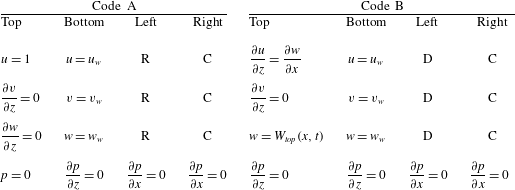
The present code is designed as an ‘AB code’ framework, with code-A for a prior zero pressure gradient turbulent boundary layer (ZPGTBL) simulation and code-B for the main separation/reattachment LES. The computational domains for both codes are of rectangular parallelepiped shape. Code-A and code-B employ the same numerical method as discussed above, but employ different boundary conditions. For comparison, table 1 lists all the boundary conditions for both code-A and code-B. The same boundary conditions are used in the two codes for the outflow boundary and the virtual wall boundary. The inflow boundary condition for code-A is generated by the recycling method (Lund, Wu & Squires Reference Lund, Wu and Squires1998). In code-A, a Dirichlet pressure boundary condition is used for the top boundary. Since code-B does not have uniform free-stream flow at the upper boundary, the most accurate boundary condition for the top boundary is to specify the normal velocity profile
 $W_{top}(x,t)$
. This type of boundary condition was used in DNS of separation in a flat-plate TBL by Na & Moin (Reference Na and Moin1998) and Skote & Henningson (Reference Skote and Henningson2002).
Boundary conditions for A and B codes. D, Dirichlet type; R, recycling method (Lund et al. Reference Lund, Wu and Squires1998); C, convective outflow.

3.2. Simulation strategy
Presently, we try to match wall conditions in experiments performed with curved upper walls using LES in rectangular parallelepiped domains. For flow where there exists a separation bubble, care is required in making comparisons between LES and the results of these experiments. Our general strategy is to design boundary conditions for code B that will reproduce flat-wall, streamwise pressure distributions close to those measured in the experiments. This, together with a parametric description that characterizes flows with separation/reattachment is now discussed in some detail.
Unlike the ZPGTBL, which has a uniform free-stream flow and only one parameter (Reynolds number), flow with separation from a flat plate will depict features that depend critically on the top boundary condition. Suppose that the form of the vertical velocity function along the top wall is given by
 $W_{top}(x/L_{p})$
, where
 $L_{P}$
is a length scale. Then for a given rectangular parallelepiped computational domain, the remaining flow parameters would be the inflow velocity
 $U_{\infty }$
, the viscosity
 ${\it\nu}$
, some measure of the boundary layer thickness
 ${\it\delta}$
and
 $L_{p}$
. For diagnosing flow results, two other parameters of interest are the length
 $L_{B}$
and the height
 $H_{B}$
of the separation bubble. Using dimensional analysis, we can then write
 $$\begin{eqnarray}{\displaystyle \frac{L_{B}}{{\it\delta}}}=F_{1}\left(Re_{{\it\delta}},{\displaystyle \frac{L_{p}}{{\it\delta}}}\right),\quad {\displaystyle \frac{H_{B}}{{\it\delta}}}=F_{2}\left(Re_{{\it\delta}},{\displaystyle \frac{L_{p}}{{\it\delta}}}\right).\end{eqnarray}$$
Generally the functional form of both
 $F_{1}$
and
 $F_{2}$
may be expected to depend on the specific form of
 $W_{top}(x/L_{p})$
.
In order to produce flow containing a separation bubble, the imposition of a streamwise pressure distribution is required. Here
 $C_{p}$
increases with the imposed APG prior to boundary-layer separation. Inside the separation bubble itself,
 $C_{p}$
will be determined by the structure the bubble flow, typically remaining approximately constant for the first part of the separation bubble, and then increasing to an apex or maximum within the incipient reattachment region. After reattachment,
 $C_{p}$
then decreases in a favourable-pressure-gradient (FPG) region to match a desired outflow boundary condition. In order to discuss this in quantitative terms, we summarize our interpretation of some prior work on the general effect of pressure gradient as follows. We consider the smooth development of
 $C_{p}(x)$
along a streamwise direction, and define two parameters
 $C_{inc}$
and
 $C_{dec}$
, the streamwise average of changes in
 $C_{p}$
during separation and reattachment, respectively, with
 $C_{inc}=|{\rm\Delta}C_{p}|_{i}/{\rm\Delta}x_{i}^{\prime }$
and
 $C_{dec}=|{\rm\Delta}C_{p}|_{d}/{\rm\Delta}x_{d}^{\prime }$
. Here the subscript ‘
 $i$
’ denotes the increasing part before separation and ‘
 $d$
’ the decreasing part after reattachment and
 ${\rm\Delta}x^{\prime }$
is the dimensionless length of the region over which
 $C_{p}$
changes, generally defined as
 ${\rm\Delta}x^{\prime }=L_{p}/{\it\delta}_{99}^{in}$
where
 ${\it\delta}_{99}^{in}$
is the 99 % boundary-layer thickness just before the onset of the imposed APG. In the present simulation the APG corresponds to the first part of
 $W_{top}(x)$
on the top boundary.
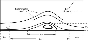
Sketch configuration of the separation-bubble flow after Perry & Fairlie (Reference Perry and Fairlie1975).
 $L_{in}$
, length of ZPG part near inlet;
 $L_{out}$
, length of ZPG part near outlet;
 $L_{P}$
length of APG part;
 $L_{B}$
, length of the bubble;
 $H_{B}$
, height of the bubble.

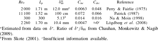
Table of parameters for experimental and DNS data.
 $C_{inc}$
and
 $C_{dec}$
correspond to the average spanwise increase and decrease in pressure coefficient
 $C_{p}$
, respectively. All
 $Re_{{\it\theta}}$
,
 $L_{p}$
and
 ${\it\delta}_{99}$
are calculated from data or scaled from figures in reference cited.

a
Estimated from data on
 ${\it\delta}^{\ast }$
. Ratio of
 ${\it\delta}^{\ast }/{\it\delta}_{99}$
from Chauhan, Monkewitz & Nagib (Reference Chauhan, Monkewitz and Nagib2009).
b From Skote (Reference Skote2001).
c Insufficient information available.
Table 2 lists our estimates of these parameters for some previous work on separation in TBL flow. We find that Perry & Fairlie (Reference Perry and Fairlie1975) has a very mild APG but a strong FPG. Patrick (Reference Patrick1987) has both a strong APG and subsequent FPG, while Lögdberg et al. (Reference Lögdberg, Angele and Alfredsson2008) has a mild APG for separation and weak FPG for reattachment. One aim of the present work is to undertake strong quantitative comparisons between our LES and some of the existing experimental studies of separation and reattachment. We first address the case of Perry & Fairlie (Reference Perry and Fairlie1975) in order to test the present wall model up to separation, and also for a mild APG followed by a strong FPG at low Reynolds number. Subsequently, we address the flow studied by Patrick (Reference Patrick1987) to evaluate the performance of the overall LES, including the present two-dimensional wall model at moderately high Reynolds number.
4. Separation bubble: Perry & Fairlie (Reference Perry and Fairlie1975)
Utilizing the above analysis, we design boundary conditions to generate flows in a parallelepiped domain which enable direct comparison with the experiments of Perry & Fairlie (Reference Perry and Fairlie1975). They used a 2.5 m long working section and a Reynolds number
 $1.25\times 10^{6}~\text{m}^{-1}$
. While Perry & Fairlie (Reference Perry and Fairlie1975) do not provide data on the state of the upstream ZPG TBL, their tabulated
 $C_{f}$
and the displacement boundary-layer thickness
 ${\it\delta}^{\ast }$
data at
 $x=0.15~\text{m}$
(the first point in the data and inside the APG part), conforms closely to the Coles–Fernholz 1 formula,
 $C_{f}/4=\log (Re_{{\it\delta}^{\ast }})/0.384+3.354$
(Nagib, Chauhan & Monkewitz Reference Nagib, Chauhan and Monkewitz2007). Thus the data at this point are chosen as scaling parameters. We note that the actual available length scale for
 $C_{p}$
is
 $L_{p}=1.7~\text{m}$
. Although the pressure gradient has still not fully recovered, this length,
 $L_{p}$
is nonetheless considered as the
 $L_{p}$
in our LES. From the above discussion, we obtain
 $Re_{{\it\theta}}=2000$
and
 $L_{p}/{\it\delta}_{99}^{in}=142$
from the experimental data.
4.1. Domain size and mesh resolution
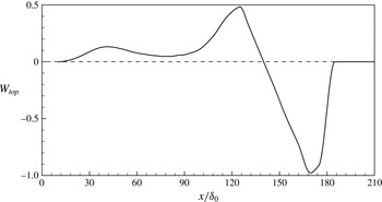
Vertical velocity distribution
 $W_{top}(x)$
used as a boundary condition on the top-wall of a rectangular parallelepiped domain for the case of Perry and Fairlie. – – – –,
 $W_{top}=0$
.

Figure 1 provides a sketch for the interpretation of the present LES in relation to the experimental conditions. This illustrates the definitions described previously, including
 $L_{p}$
,
 $L_{B}$
,
 $H_{B}$
and
 $Re_{{\it\delta}}$
. We identify two distinct parts or portions of the ZPGTBL, before separation and after reattachment, with lengths defined as
 $L_{in}$
and
 $L_{out}$
, respectively. These connect to the non-zero pressure gradient part of the flow. These two ZPG parts are used to accommodate the flow to ensure that the inflow and outflow boundary conditions have minimal impact on the flow within the non-zero pressure gradient region. In figure 1 the experimental configuration is sketched as a dual-roof top wall which generates first the APG followed by the FPG. The present LES employs instead a parallelepiped box. The present strategy is then to match the given experimental
 $C_{p}(x)$
data, to be discussed subsequently, on the bottom wall by tuning
 $W_{top}(x)$
. This is done by trial and error using a rough, simple potential flow model using sinks, sources and vortices as a guide. The final
 $W_{top}(x/{\it\delta}_{0})$
used for the Perry & Fairlie (Reference Perry and Fairlie1975) experiment is plotted in figure 2.
We use a nominal boundary-layer thickness
 ${\it\delta}_{0}$
as a length scale and fix the 99 % boundary-layer thickness at the beginning of the APG region as
 $1.2{\it\delta}_{0}$
. The domain length in the streamwise direction was set to be
 $216{\it\delta}_{0}$
, with
 $W_{top}(x/L_{p})$
enforced in a length
 $L_{p}=170{\it\delta}_{0}$
. This numerical test section joins an upstream ZPG part with
 $L_{in}=10{\it\delta}_{0}$
, which is for the development of the inflow, and is connected to a second, downstream ZPG part with
 $L_{out}=36{\it\delta}_{0}$
. The ZPG parts are designed to ensure that the influence of vertical velocity enforcement does not reach the inflow and outflow boundaries in the streamwise direction. As a check, we plot isolines of the mean (in the sense of spanwise and time-averaged) vertical velocity in the
 $(x,z)$
plane of the simulation domain in figure 3 for a typical LES. It can be seen that the isolines of
 $w=\pm 0.01$
, which correspond to approximately 1 % of the maximum vertical velocity, do not extend to either the inflow or outflow boundaries.
Isolines of spanwise mean vertical velocity
 $W$
.
 $W=0.01$
describes the upper limit of the desired vertical velocity for an acceptable upstream influence of the APG.

Isolines of mean streamwise velocity
 $U$
(– – – –) and streamlines of mean velocity (—— with arrows). Line — ⋅ — is the isoline of
 $U=0.4595$
, a visualization of the saddle point.

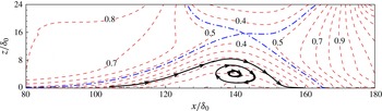
The domain size in the wall-normal direction should be restricted by a fully-potential flow top boundary criterion. We ensure that the saddle point of the
 $\tilde{u} (x,y)$
field above the separation bubble is located within the computational domain. A similar criterion was used by Na & Moin (Reference Na and Moin1998). Figure 4, in which the dashed lines are the isolines of mean streamwise velocity while the solid lines are the streamlines of the mean velocity, illustrates this criterion. The domain in the
 $z$
-direction is presently
 $24{\it\delta}_{0}$
. This is also where the vertical velocity boundary condition
 $W_{top}(x)$
, shown in figure 2, is imposed.
There is no straightforward criterion available for the domain size in the spanwise direction. Ideally the spanwise domain should have sufficient space for the development of the largest turbulent structures. However, as wall-modelled LES cannot precisely capture these largest structures, the present strategy is to compare the averaged properties from results predicted with a different spanwise domain. We start with a spanwise domain
 $12{\it\delta}_{0}$
, which is comparable to the domain size of
 $9.8{\it\delta}_{0}$
in Na & Moin (Reference Na and Moin1998).
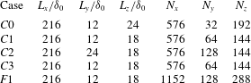
Presently, several LES cases are implemented in order to assess the influence of domain-size and resolution; see table 3. Three coarse mesh cases test domain size, with
 $C_{0}$
the baseline domain discussed above,
 $C_{1}$
a smaller domain in the wall-normal direction
 $L_{z}=18{\it\delta}_{0}$
and
 $C_{2}$
is the doubled spanwise domain. Case
 $F_{1}$
is a fine mesh case for assessing mesh resolution. Note that for all cases with
 $L_{z}=18{\it\delta}_{0}$
, the vertical velocity at
 $z=18{\it\delta}_{0}$
obtained from case
 $C_{0}$
is imposed on the top boundary. The Reynolds number is set to
 $Re_{{\it\theta}}^{in}=2000$
with superscript ‘
 $in$
’ denoting just upstream of the region where the vertical velocity boundary condition is imposed. This is implemented by adjusting the inflow boundary-layer thickness in code-A. For most LES, model I was used for calculation of
 ${\it\theta}_{0}$
. One case was performed using model II.
Wall pressure coefficient
 $C_{p}$
: ▫, experiment (Perry & Fairlie Reference Perry and Fairlie1975), – – – –, case
 $C0$
; — ⋅ —, case
 $C1$
; — ⋅ ⋅ —, case
 $C2$
;
 $\cdots \cdots$
, case
 $C3$
; ——, case
 $F1$
.

Time evolution of maximum height of the backflow region,
 $h_{B}$
. First
 $3T_{t}$
is the start-up transient followed by
 $5T_{t}$
for stabilizing the flow and then a final
 $10T_{t}$
for diagnostics and output.
 $T_{t}$
is a typical particle transit time across the domain.

Boundary-layer thickness parameters up to separation. Symbols for experiment (Perry & Fairlie Reference Perry and Fairlie1975), lines for LES results, case
 $F1$
. ▫,
 $Re_{{\it\theta}}$
, ○,
 $H$
. ——,
 $Re_{{\it\theta}}$
, - - - -,
 $H$
.

LES performed for Perry & Fairlie (Reference Perry and Fairlie1975) flow: three coarse-mesh cases with different spanwise and wall-normal domain dimensions, and one finer-mesh case,
 $F1$
.
 $Re_{{\it\theta}}^{in}=2000$
is held constant.
 $C3$
is an extension of
 $C1$
with using model II.

4.2. Wall streamwise pressure distribution
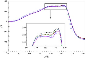
As shown in figure 5,
 $C_{p}$
distributions from the various LES are similar and they all match reasonably with the experimental measurements of Perry & Fairlie (Reference Perry and Fairlie1975). Figure 5 also includes a close-up of
 $C_{p}$
in the separated region. We find that the differences between cases are within model error, and that the fine mesh case
 $F1$
shows somewhat better agreement with experimental data than the coarse mesh cases. We note also that the LES using model I for
 ${\it\theta}_{0}$
is very close to that using model II at a similar resolution.
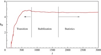
The initial conditions used for both code A and code B are zero-pressure gradient results from previous LES at the same Reynolds number. The vertical velocity boundary condition on the top boundary is applied instantaneously from
 $t=0$
. Figure 6 shows the time evolution of the maximum height of the backflow region
 $h_{B}$
. This rapidly increases from zero, reaching a maximum at about three times a characteristic flow time
 $3T_{t}$
where
 $T_{t}$
refers to the time required for a typical free-stream particle to transit the full flow domain. At about
 $t=8T_{t}$
, the flow is considered to reach statistical steady state, and simple average diagnostics are implemented in the next
 $10T_{t}$
period.
4.3. Boundary-layer thickness and skin-friction distribution
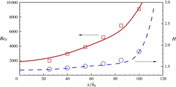
Because Perry & Fairlie (Reference Perry and Fairlie1975) recorded boundary-layer flow data prior to flow separation, we focus first on the APG of the flow. Figure 7 shows the streamwise variation of both
 $Re_{{\it\theta}}$
and the shape factor
 $H\equiv {\it\delta}^{\ast }/{\it\theta}$
, respectively versus
 $x/{\it\delta}_{0}$
prior to separation. It can be seen that our LES generally matches the
 $Re_{{\it\theta}}$
number development in this region.
Skin friction coefficient
 $C_{f}$
. Symbols for experiments by Perry & Fairlie (Reference Perry and Fairlie1975), lines for present LES. ▫,
 $C_{f}$
; ○, separation point; ▵, reattachment point; – – – –, case
 $C0$
; — ⋅ —, case
 $C1$
; — ⋅ ⋅ —, case
 $C2$
;
 $\cdots \cdots$
, case
 $C3$
; ——, case
 $F1$
. Horizontal dashed line indicates
 $C_{f}=0$
.

The skin friction
 $C_{f}$
is defined presently as
 $$\begin{eqnarray}C_{f}\equiv {\displaystyle \frac{|\overline{{\it\tau}_{w,x}}|}{{\textstyle \frac{1}{2}}\,{\it\rho}\,U_{\infty }^{2}}}={\displaystyle \frac{2{\it\nu}}{U_{\infty }^{2}}}\,|\overline{{\it\eta}_{0}\cos {\it\theta}_{0}}|,\end{eqnarray}$$
where the overline refers to a time-spanwise average, and we note that, by definition,
 $C_{f}\geqslant 0$
always. This is perhaps the most important flowfield parameter in our wall-modelled LES as we directly solve for
 ${\it\eta}_{0}$
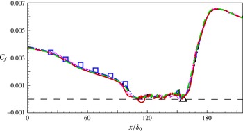
from the ODE (2.14). Figure 8 plots
 $C_{f}$
versus
 $x/{\it\delta}_{0}$
. It is seen that our LES can reasonably capture the
 $C_{f}$
development in the streamwise development prior to separation where measurements were recorded. This means the whole APG TBL development before separation is accurately represented by the LES. This result is consistent with the APG TBL simulation performed by Inoue et al. (Reference Inoue, Pullin, Harun and Marusic2013), which uses Dirichlet streamwise velocity and pressure boundary conditions. Note that in Inoue et al. (Reference Inoue, Pullin, Harun and Marusic2013), a one-dimensional wall model is used and only a small APG region is implemented. Again it can be seen that the
 $C_{f}(x)$
variation using model I for
 ${\it\theta}_{0}(x,y,t)$
is very close to that obtained using model II. This is evidence that the overall LES is relatively insensitive to this choice. Hence subsequently, all LES discussed presently utilize the simpler model I.
Two points plotted in figure 8 are the separation point and reattachment point obtained from experiment from mean-flow streamlines. In the present simulation, the two-dimensional wall model enables calculation of
 $C_{f}$
up to and through separation. For three-dimensional flow, even when statistically stationary in some sense, a ‘separation point’ is not generally defined. But since the present flow is driven by boundary conditions that have no variation in the
 $y$
or spanwise direction, it is expected to be statically stationary and two-dimensional in the time-wise mean. Hence presently, the separation and reattachment points in
 $x$
are defined as those points where the time-spanwise averaged
 $x$
-shear stress
 $\overline{{\it\tau}_{w,x}}$
, as calculated from the ODE, changes sign. As shown in figure 8, this measure of the separation and reattachment points agrees well with the experimental results.
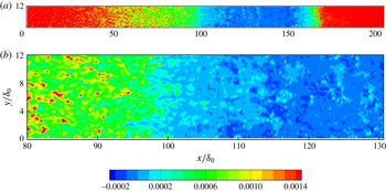
The separation/reattachment flow is highly unsteady and far from two dimensional. This is illustrated in figure 9 which shows an
 $x{-}y$
plane plot, on the plane
 $z=0$
, of the instantaneous (at a particular time) streamwise component of wall shear stress
 ${\it\tau}_{w,x}$
. The whole-domain plot on the figure 9(a) shows the spatially non-uniform character of a typical instantaneous distribution of
 ${\it\tau}_{w,x}$
. From the close-up plot, we can see that separation is not well defined in an instantaneous image. In the region surrounding the mean separation line as defined previously, at about
 $x/{\it\delta}_{0}=112$
, the instantaneous field of
 ${\it\tau}_{w,x}$
is highly irregular, showing patches and areas of both positive and negative sign over a region of extent many
 ${\it\delta}_{0}$
in the streamwise direction. This feature is perhaps associated with the moderate APG for this case. In contrast, further downstream, the
 ${\it\tau}_{w,x}$
field appears to be more ordered in the reattachment region where the strong FPG enables recovery of the skin friction to quite strong positivity.
4.4. Bubble size and velocity profile
To compare data that characterizes the extent of the separation bubble, we compare both
 $L_{B}/{\it\delta}_{99}^{in}$
and
 $H_{B}/{\it\delta}_{99}^{in}$
in table 4. Note that here
 $L_{B}/{\it\delta}_{99}^{in}$
is defined by the separation point and reattachment point from
 $C_{f}=0$
.
 $H_{B}/{\it\delta}_{99}^{in}$
is evaluated from the maximum height of the enveloping line of the separation bubble. Both the bubble length and height in all simulations are close to the experimental data within a few per cent.
Contour plot of the instantaneous
 ${\it\tau}_{w,x}(x,y)$
. Case
 $F1$
of table 3. (a) The whole domain. (b) Close-up near separation. Both figures use the key shown.

Comparison of bubble size with experimental data from Perry & Fairlie (Reference Perry and Fairlie1975): length of the bubble
 $L_{B}$
and height of the bubble
 $H_{B}$
. Length scale
 ${\it\delta}_{99}^{in}$
set to be
 ${\it\delta}_{99}$
before APG part of flow.

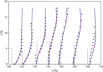
Comparison of velocity profiles. ▪, Experimental data Perry & Fairlie (Reference Perry and Fairlie1975); ——, LES case
 $C1$
; – – – –, LES case
 $F1$
.

Figure 10 shows the mean streamwise velocity profile at different locations. These match those of the experiment, with two upstream of the bubble (
 $x/{\it\delta}_{0}=102.6,110.6$
), four points inside the bubble (
 $x/{\it\delta}_{0}=121.6,131.0,139.4,150.0$
) and one final point downstream the bubble (
 $x/{\it\delta}_{0}=160.0$
). We plot velocity profiles for two cases, a solid line for
 $C1$
and dashed line for
 $F1$
. It can be found that, in the region upstream of the bubble, the velocity profiles obtained from LES are in reasonably good agreement with experiments.
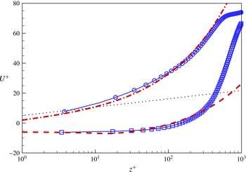
Skote & Henningson (Reference Skote and Henningson2002) propose a model for mean velocity scaling in the separation region. Prior to separation, their mean velocity is given by
 $$\begin{eqnarray}U^{+}={\displaystyle \frac{1}{{\it\kappa}}}\left(\ln z^{+}-2\ln {\displaystyle \frac{\sqrt{1+{\it\lambda}z^{+}}+1}{2}}+2(\sqrt{1+{\it\lambda}z^{+}}-1)\right)+B,\end{eqnarray}$$
while the velocity profile inside the separation region is
 $$\begin{eqnarray}U^{+}={\displaystyle \frac{1}{{\it\kappa}}}\left(2\sqrt{{\it\lambda}z^{+}-1}-2\arctan (\sqrt{{\it\lambda}z^{+}-1})\right)+C,\end{eqnarray}$$
where
 $$\begin{eqnarray}U^{+}={\displaystyle \frac{u}{u_{{\it\tau}}}},\quad {\it\lambda}=\left({\displaystyle \frac{u_{p}}{u_{{\it\tau}}}}\right)^{3},\quad u_{p}=\left({\it\nu}\left.{\displaystyle \frac{\text{d}p}{\text{d}x}}\right|_{z=0}\right)^{1/3},\quad u_{{\it\tau}}=\sqrt{2C_{f}}.\end{eqnarray}$$
Comparison of velocity profiles:
 $\cdots \cdots$
, log line
 $U^{+}=(1/0.378)\ln z^{+}+4.08$
(Inoue & Pullin Reference Inoue and Pullin2011); — ⋅ —, (4.2); – – – –, (4.3); —— with symbols, LES results. ○,
 $x/{\it\delta}_{0}=102.6$
; ▫,
 $x/{\it\delta}=121.6$
.

The present LES is compared with these scalings in figure 11 where we use the same parameters as suggested in Skote & Henningson (Reference Skote and Henningson2002):
 ${\it\kappa}=0.41$
,
 $B=1.5$
and
 $C=-7$
. In determining the LES profiles, we presently use
 $u_{{\it\tau}}$
defined in (4.4). This is strictly for the present comparison and is not the same as the wall-model definition of
 $u_{{\it\tau}}$
given by the second of (2.9). We compare two velocity profiles at
 $x/{\it\delta}_{0}=102.6$
and
 $121.6$
, which are the first and third velocity profiles in figure 10. The velocity profile at
 $x/{\it\delta}_{0}=102.6$
, which is in the APG region, agrees quite well with (4.2), but is different from the classical log law. The velocity profile within the separated region also matches (4.3) reasonably well up to
 $z^{+}\approx 350$
, implying that the Skote and Henningson theory is valid for weakly separated flow.
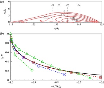
Velocity in backflow region. (a) Isolines of mean streamwise velocity of backflow,
 $U<0$
(contour of
 $U$
). Velocity probed at
 $P1$
,
 $P2$
,
 $P3$
and
 $P4$
(vertical dash lines) are extracted for (b). (b) Scaled velocity. ——, Scaling equation (4.5), Simpson (Reference Simpson1983); – – – – with symbols, LES results. ▵,
 $P1$
; ▫,
 $P2$
; ○,
 $P3$
; ♢,
 $P4$
(comparison of scaled
 $U$
).

For the region downstream of separation, Simpson (Reference Simpson1983) suggests a scaling formula to describe the velocity profile of the main backflow region. In this scaling, the maximum negative velocity
 $U_{N}$
and its distance from the wall
 $N$
are two basic parameters. Simpson’s equation, which covers the region of
 $0.02<z/N<1.0$
with
 $z$
the wall-normal coordinate, is given by
 $$\begin{eqnarray}{\displaystyle \frac{U}{U_{N}}}=A\left({\displaystyle \frac{z}{N}}-\ln \left|{\displaystyle \frac{z}{N}}\right|-1\right)-1\end{eqnarray}$$
with
 $A=0.3$
. To compare with this scaling formula, contours of the backflow velocity are first plotted in figure 12(a). This shows that the present LES can capture the maximum negative velocity at about
 $135<x/{\it\delta}_{0}<145$
. The streamwise velocity at four positions are extracted and plotted in figure 12(b), with
 $x/{\it\delta}_{0}=133.5(P1)$
,
 $136.5$
,
 $140$
and
 $145$
. We find that at position
 $P2$
, which is a good example from the LES owing to obvious maximum backflow velocity and sufficient mesh points for
 $z<N$
, the LES results agree quite well with the formula. For
 $P1$
, there is interaction of different isolines. This complexity raises the backflow velocity to somewhat above the theory. The velocity profiles at position
 $P3$
also agrees well with the scaling formula. Comparison of
 $P2$
and
 $P3$
shows that only the first two near-wall points deviate from the formula, with fair agreement for other points. Except for
 $P4$
, where there are only three points under the maximum negative velocity, the present LES results are broadly consistent with (4.5).
4.5. Discussion
We have argued that the present wall model can accurately model the near wall flow before separation, reasonably postdict the separation and reattachment points and show good agreement for the velocity profiles. Referring to the velocity slip component of the wall model defined by (2.17), we find that for the LES corresponding to the Perry & Fairlie (Reference Perry and Fairlie1975) flow, use of
 $Re_{{\it\theta}}=2000$
results in a small
 $h_{0}^{+}$
within the separation bubble. In particular, for both the coarse and fine mesh LES,
 $h_{0}^{+}(x,y,t)$
, which fluctuates in time because the calculated
 $u_{{\it\tau}}(x,y,t)$
fluctuates, satisfies
 $h_{0}^{+}(x,y,t)<h_{{\it\nu}}^{+}$
in more than 99 % of realizations. From (2.17) this then means that the linear form of the slip velocity is overwhelmingly used within the separated region. Next, we consider a second case from Patrick (Reference Patrick1987), at sufficiently high Reynolds numbers,
 $Re_{{\it\theta}}=11\,000$
, which gives
 $h_{0}^{+}>h_{{\it\nu}}^{+}$
within the separation bubble.
5. Separation bubble: Patrick (Reference Patrick1987)
The experiment of Patrick (Reference Patrick1987) differs from Perry & Fairlie (Reference Perry and Fairlie1975), owing to the relative size of the separation bubble in comparison to the scale of the confining duct geometry. From table 2, we find that
 $L_{p}/{\it\delta}_{99}^{in}$
in Perry & Fairlie (Reference Perry and Fairlie1975) is almost ten times that in Patrick (Reference Patrick1987). Differences of
 $C_{inc}$
are similar. In other words, Patrick (Reference Patrick1987) provides a separation process induced by a very strong APG. This tends to generate a separation region that is more confined in the streamwise direction and somewhat more ordered than the Perry & Fairlie (Reference Perry and Fairlie1975) flow. It also implies a
 $W_{top}(x)$
boundary condition on the upper wall with very strong streamwise gradients, which can potentially reduce the robustness of the LES.
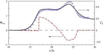
Case of Patrick: vertical velocity on the top boundary
 $W_{top}$
(— ⋅ —) and mean wall-pressure coefficient
 $C_{p}$
(——). ▫, Experiment, Patrick (Reference Patrick1987).

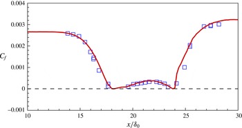
Streamwise variation of skin-friction coefficient
 $C_{f}$
.▫, Experiment, Patrick (Reference Patrick1987); ——, LES; – – – –,
 $C_{f}=0$
.

In designing the LES, a similar procedure to that used previously is repeated here to determine the dimensions of the computational domain in streamwise, spanwise and wall-normal directions. The domain used is
 $36{\it\delta}_{0}\times 12{\it\delta}_{0}\times 3.2{\it\delta}_{0}$
. In the streamwise direction, the first
 $L_{in}=10{\it\delta}_{0}$
is a zero-pressure-gradient flow which then connects to the varying pressure gradient part with
 $L_{p}=15.2{\it\delta}_{0}$
. The final subdomain, which is approximately
 $L_{out}=11{\it\delta}_{0}$
, is used to adapt the flow back to the ZPG state. The mesh used, which has similar resolution to that of case
 $F1$
, is
 $384\times 128\times 96$
. The vertical velocity imposed on the top boundary is shown in figure 13. It can be seen that the
 $C_{p}(x)$
distribution on the wall, which is derived from the actual LES, captures approximately the streamwise variation of pressure in the experiment.
Figure 14 compares the
 $C_{f}$
of the LES and experiment. This shows that the present LES can capture well almost all variations within the separated flow. In the approach to separation, the decrease of
 $C_{f}$
due to the steep APG is reasonably modelled. The LES also reproduces well the
 $C_{f}$
variation inside the bubble, with good agreement between experiment and LES. In the LES the first grid point is beyond the viscous sublayer, with
 $h_{0}^{+}>h_{{\it\nu}}^{+}$
in more than 80 % of realizations. This demonstrates the present effectiveness of a simple linear model given in (2.17) for regions of local back flow.
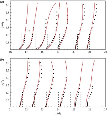
Comparison of mean streamwise velocity profiles at different locations. ▫, Experimental data Patrick (Reference Patrick1987); – – – –, reference of streamwise locations; ——, LES results.

In figure 15 we also compare the streamwise velocity profiles at several streamwise locations with the experimental measurements of Patrick (Reference Patrick1987). Results show that the velocity profile predicted by LES generally follows the experimental data.
6. Results and discussion
6.1. Separation bubble
It is of interest to discuss some other features of the separation bubble flows of both Perry & Fairlie (Reference Perry and Fairlie1975) and Patrick (Reference Patrick1987). As discussed previously, the case of Perry and Fairlie has a mild APG combined with a strong FPG, and its
 $C_{f}$
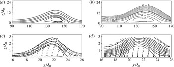
from the LES shows a strong streamwise asymmetry in figure 8. This behaviour can be observed in the bubble shape, as shown in figure 16(a), where we find the bubble is not perfectly symmetric, being slightly lifted towards the downstream part of the flow domain. Physically, it is reasonable that the bubble is not symmetric owing to the unsymmetrical pressure gradient. Interestingly, this feature is not present in all cases. For the Patrick flow, the
 $C_{f}(x)$
variation of figure 14, while not perfectly symmetric, is more so than in the case of Perry and Fairlie. The bubble shape is also approximately symmetric. Considering the sharp pressure gradient near separation, a rather large bubble is generated. In figure 16, experiment and LES look reasonably similar near and inside the separation bubble.
Comparison of separation bubble shape. (a) LES for the case of Perry & Fairlie (Reference Perry and Fairlie1975); (b) experiment by Perry & Fairlie (Reference Perry and Fairlie1975); (c) LES for the case of Patrick (Reference Patrick1987); (d) experiment by Patrick (Reference Patrick1987).

Effect of Reynolds number: ——,
 $Re_{{\it\theta}}^{in}=2000$
; – – – –,
 $Re_{{\it\theta}}^{in}=8000$
; — ⋅ —,
 $Re_{{\it\theta}}^{in}=16\,000$
; — ⋅ ⋅ —,
 $Re_{{\it\theta}}^{in}=10^{5}$
; ▫, from experimental data of Perry & Fairlie (Reference Perry and Fairlie1975). (a)
 $C_{f}$
versus
 $x/{\it\delta}_{0}$
; (b)
 $\overline{h_{0}^{+}}$
versus
 $x/{\it\delta}_{0}$
; (c)
 ${\it\beta}$
versus
 $x/{\it\delta}_{0}$
.

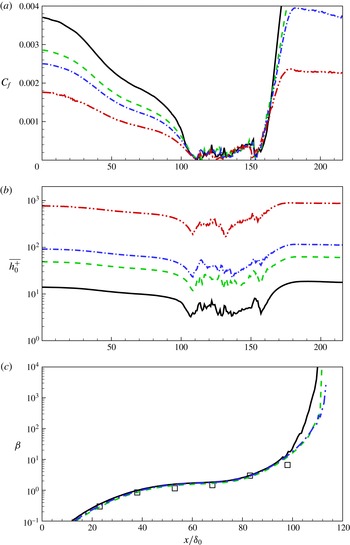
Another interesting effect is the change of bubble size due to Reynolds number. The case of Perry and Fairlie was extended to three further LES with
 $Re_{{\it\theta}}^{in}=8000$
, 16 000 and
 $10^{5}$
. The same numerical set-up as in case
 $C1$
was used. In figure 17(a), the
 $C_{f}(x)$
variation is qualitatively similar for all cases. As
 $Re_{{\it\theta}}^{in}$
increases, the values of
 $C_{f}$
before separation and after reattachment reduce substantially at a given
 $x$
, consistent with the effect of increasing Reynolds number on an attached flow TBL. In contrast, inside the separation bubble, differences in
 $C_{f}(x)$
are relatively smaller between the various cases, suggesting an interior bubble flow that is only weakly dependent on Reynolds number over a broad range.
To compare the wall-model behaviour in cases with different Reynolds number, the variation of
 $\overline{h_{0}^{+}}$
versus
 $x/{\it\delta}_{0}$
is shown in figure 17(b) for the Perry–Fairlie flow. The quantity
 $h_{0}^{+}(x,y,t)$
is dynamically calculated at every wall point. Here, its mean diagnostic is defined as
 $$\begin{eqnarray}\overline{h_{0}^{+}}(x)\equiv {\displaystyle \frac{h_{0}\sqrt{\overline{u_{{\it\tau}}^{2}}}}{{\it\nu}}}=h_{0}\sqrt{{\displaystyle \frac{\overline{{\it\eta}_{0}}}{{\it\nu}}}}.\end{eqnarray}$$
The average of
 ${\it\eta}_{0}$
is implemented in both the spanwise direction and in time. It is interesting that
 $\overline{h_{0}^{+}}$
does not approach zero even near the separation and reattachment points. This is reasonable as we would expect that
 ${\it\eta}_{0}(x,y,t)$
, which is proportional the magnitude of the skin-friction vector, would be zero only at isolated critical points. Since we have fixed relation
 $h^{+}=0.68/0.18h_{0}^{+}$
, the behaviour of
 $h^{+}$
is not shown. The variation of
 $\overline{h_{0}^{+}}(x)$
for the Patrick flow is similar to that of figure 17(b).
An issue of some interest is the effect of the boundary condition (2.19) used presently for the wall-normal velocity. For the LES of the Perry–Fairlie flow, we find that at the virtual wall,
 $\text{Prob}:\{|\tilde{w}|_{h_{0}}/\tilde{q}|_{h_{0}}>0.05\}\approx 0.07$
,
 $\text{Prob}:\{|\tilde{w}|_{h_{0}}/\tilde{q}|_{h_{0}}\}>0.1\approx 0.038$
and
 $\text{Prob}:\{|\tilde{w}|_{h_{0}}/\tilde{q}|_{h_{0}}>0.2\}\approx 0.02$
, while for the Patrick flow the corresponding results are
 $\text{Prob}:\{|\tilde{w}|_{h_{0}}/\tilde{q}|_{h_{0}}>0.05\}\approx 0.097$
,
 $\text{Prob}:\{|\tilde{w}|_{h_{0}}/\tilde{q}|_{h_{0}}>0.1\}\approx 0.061$
and
 $\text{Prob}:\{|\tilde{w}|_{h_{0}}/\tilde{q}|_{h_{0}}>0.2\}\approx 0.038$
. These values are small but not negligible and are probably associated with local regions of small
 $|\boldsymbol{{\it\tau}}_{w}|$
within the large-scale separated flow. When, however, (2.19) is replaced with
 $|\tilde{w}|_{h_{0}}=0$
, we find LES results for example for the
 $C_{f}(x)$
distribution (not shown) that are little different to those shown presently.
In passing, we note the large-scale Reynolds numbers
 $Re_{B}\equiv U_{\infty }\,L_{b}/{\it\nu}$
for the present separation-bubble flows. For the Perry–Fairlie flow with
 $Re_{{\it\theta}}^{in}=2\times 10^{3},8\times 10^{3}$
,
 $1.6\times 10^{4}$
and
 $10^{5}$
, we find
 $Re_{B}=5.3\times 10^{5},2.1\times 10^{6},4.2\times 10^{6}$
and
 $4.2\times 10^{7}$
, respectively. For the Patrick case with
 $R_{{\it\theta}}=1.1\times 10^{4}$
, then
 $Re_{B}=6\times 10^{5}$
. This shows that
 $Re_{B}$
for the two experiments are almost the same. This is because for the Patrick case,
 ${\it\theta}$
is six times larger than for the Perry and Fairlie flow, but the bubble length is five times smaller. These values of
 $Re_{B}$
serve to indicate that we are performing LES at substantial values of the large-scale Reynolds number.
For quantifying different APG flows over a range of Reynolds number, a commonly used metric is the non-dimensional pressure gradient parameter
 $$\begin{eqnarray}{\it\beta}={\displaystyle \frac{{\it\delta}^{\ast }}{{\it\tau}_{w}}}{\displaystyle \frac{\text{d}P}{\text{d}x}},\end{eqnarray}$$
which is plotted versus
 $x/{\it\delta}_{0}$
in figure 17(c). Results show that all three cases plotted collapse into a curve, which is consistent with results by Inoue et al. (Reference Inoue, Pullin, Harun and Marusic2013). When the TBL is lifted by the APG, we observe that
 ${\it\beta}$
in the lowest Reynolds number case first lifts upwards and then reaches separation. This implies that the separation bubble will shrink with increasing Reynolds number, although this effect is very slow. Lastly, we also observe that the difference between
 $Re_{{\it\theta}}^{in}=8000$
and
 $Re_{{\it\theta}}^{in}=16\,000$
is smaller than the difference between
 $Re_{{\it\theta}}^{in}=2000$
and
 $Re_{{\it\theta}}^{in}=8000$
. The LES for
 $Re_{{\it\theta}}^{in}=10^{5}$
shows differences in
 ${\it\beta}(x)$
compared with
 $Re_{{\it\theta}}^{in}=16\,000$
of order the plot-line thickness and is therefore not shown.
6.2.
$h{-}{\it\lambda}$
relation

A correlation in an
 $h{-}{\it\Lambda}$
plane has been suggested to demarcate the regions of separation where
 $h=(H-1)/H$
with
 $H\equiv {\it\delta}^{\ast }/{\it\theta}$
and
 ${\it\Lambda}\equiv {\it\delta}^{\ast }/{\it\delta}_{99}$
. Previous studies have identified two important lines on
 $h{-}{\it\Lambda}$
plots. The line
 $h=1.5{\it\Lambda}$
was discussed by Simpson (Reference Simpson1989), who stated that the data of Perry & Schofield (Reference Perry and Schofield1973) supported the hypothesis that this characterized a path for detaching flow. Another line is
 $h=1/(2-{\it\Lambda})$
proposed by Sanborn & Kline (Reference Sanborn and Kline1961). They suggested that at a given
 ${\it\Lambda}$
,
 $h$
greater than this value would indicate appreciable intermittent backflow. For a more detailed discussion of the
 $h{-}{\it\Lambda}$
plane, see Simpson (Reference Simpson1989).
Comparison of mean velocity profile parameters. In (a) and (b), ——, Perry and Schofield correction; – – – –, Sanborn and Kline relation. In (a) and (c), ▪ with line for LES results of case
 $F1$
. (a)
 $h{-}{\it\Lambda}$
plot for case by Perry & Fairlie (Reference Perry and Fairlie1975). — ⋅ — for
 $C_{f}$
; horizontal line for
 $C_{f}=0$
; (b)
 $h{-}{\it\Lambda}$
plot for case by Patrick (Reference Patrick1987). ▫, experimental data; — ⋅ —, LES result; (c) plot of
 $h(2-{\it\Lambda})$
versus
 $\overline{{\it\tau}_{u,x}}$
. Horizontal line for
 $h(2-{\it\Lambda})=1$
and vertical line for
 $\overline{{\it\tau}_{w,x}}=0$
.

Figure 18(a) plots the whole path of case
 $C2$
in the
 $h{-}{\it\Lambda}$
plane for the Perry & Fairlie (Reference Perry and Fairlie1975) flow. For interpretation purposes,
 $C_{f}$
is also plotted. The near inflow part, which includes the ZPG portion and subsequent APG part, develops from point A to point B. Here point B is the first point where our LES falls onto the Perry & Schofield (Reference Perry and Schofield1973) line. Point C, corresponding to zero skin friction, which is followed by mean backflow, corresponds closely to the Sanborn–Kline relation, as does the reattachment point D. Between these two points, the LES
 $h{-}{\it\Lambda}$
plot satisfies the Sanborn–Kline relation criterion. After reattachment, the flow further develops, and the LES
 $h{-}{\it\Lambda}$
path deviates somewhat from the Perry and Schofield correlation. The recovery of the flow near outflow to the ZPG state can be seen where the LES
 $h{-}{\it\Lambda}$
path almost closes near point A.
Figure 18(b) compares measurements by Patrick with the present LES. Note that points E and F, which are the separation point and the reattachment points, respectively, agree well with the Sanborn–Kline relation and again the LES
 $h{-}{\it\Lambda}$
path satisfies the Sanborn–Kline relation in the separated flow region. Although LES cannot exactly reproduce the experimental
 $h{-}{\it\Lambda}$
path, both are close to the Perry and Schofield correlation. A plot of
 $h(2-{\it\Lambda})$
versus
 $\overline{{\it\tau}_{w,x}}$
is provided in figure 18(c) to illustrate the interaction points between LES and Sanborn–Kline relation.
7. Conclusion
The present work develops a two-dimensional virtual-wall model designed to model in LES, both streamwise and spanwise fluctuating skin-friction properties in a turbulent wall-bounded flow that may include regions of separated flow. This wall model is a natural extension of the virtual-wall model of Chung & Pullin (Reference Chung and Pullin2009) discarding the strong assumption of near-wall flow in the virtual-wall layer along the outer streamwise direction. Starting from both components of the wall-parallel momentum equations, and assuming local inner scaling for the magnitude of the filtered, instantaneous, wall-parallel velocity up to the first wall-normal grid point, then an ODE for the wall-normal gradient of the wall-parallel fluid speed at the wall, or equivalently the square of the wall skin-friction velocity, can be obtained. Aligning the slip velocity on the virtual wall with the skin-friction vector locally at every wall point, we obtain a self-consistent and robust wall model capable of accommodating backflow with respect to an outer free-stream flow direction.
The wall model is implemented in LES for two flows, Perry & Fairlie (Reference Perry and Fairlie1975) and Patrick (Reference Patrick1987), that exhibit separation and reattachment of a turbulent boundary layer and the subsequent production of a structured separation bubble that is two-dimensional in the mean. Owing to non-equilibrium effects, the skin friction coefficient
 $C_{f}$
along the wall generally shows a somewhat complex behaviour: first decreasing up to separation, then maintaining a small magnitude within a separation bubble and finally recovering in the reattached portion of the flow. This spatial-varying behaviour presents a challenging scenario for LES. The present wall model is found to reasonably reproduce
 $C_{f}$
for both the medium Reynolds number case of Perry & Fairlie (Reference Perry and Fairlie1975) and the higher Reynolds number flow studied by Patrick (Reference Patrick1987). The present LES also reproduces other features of the separated flow including the variation in the streamwise direction of the pressure-gradient parameter
 ${\it\beta}(x)$
and the Reynolds number
 $Re_{{\it\theta}}(x)$
based on the boundary-layer momentum thickness prior to separation, the scale and shape of the separation bubble, wall-normal streamwise velocity profiles and features of the wall-flow in a
 $h{-}{\it\lambda}$
plane. The LES can be extended to quite high Reynolds number flow, presently
 $Re_{{\it\theta}}=10^{5}$
. This indicates that the effect of increasing Reynolds number on the skin friction variation is substantial outside the separation bubble but small within the bubble. Further, the effect of increasing Reynolds number on the streamwise size of the separation bubble, when the imposed wall pressure profile is fixed, appears to be small.
Although the present wall model has been developed and implemented in simple Cartesian geometry for plane walls, these constraints can be relaxed. In principle, our approach to wall-modelling for LES can be extended to a system of general coordinates on a generally curved wall with two-dimensional curvature. This suggests further applications both attached and separated flows past streamlined and bluff bodies.
Acknowledgements
W.C. and R.S. were supported by the KAUST Office of Competitive Research Funds (OCRF) under Award No. URF/1/1394-01. D.I.P. was partially supported under KAUST OCRF Award No. URF/1/1394-01 and partially by NSF award CBET 1235605.
Appendix A. Equation for
${\it\theta}_{0}$

Here we derive an equation for
 ${\it\theta}_{0}$
, the angle of the shear-stress vector at the wall. Define
 ${\it\theta}$
generally as
 $$\begin{eqnarray}{\it\theta}=\tan ^{-1}\left({\displaystyle \frac{v}{u}}\right),\quad -{\rm\pi}<{\it\theta}\leqslant {\rm\pi},\end{eqnarray}$$
and
 ${\it\theta}_{0}\equiv {\it\theta}_{z\rightarrow 0}$
. So
 $$\begin{eqnarray}{\displaystyle \frac{\partial {\it\theta}}{\partial t}}=-{\displaystyle \frac{1}{q}}\,\sin {\it\theta}\,{\displaystyle \frac{\partial u}{\partial t}}+{\displaystyle \frac{1}{q}}\,\cos {\it\theta}\,{\displaystyle \frac{\partial v}{\partial t}},\quad q^{2}=u^{2}+v^{2},\end{eqnarray}$$
where
 $\sin {\it\theta}=u/q$
,
 $\cos {\it\theta}=v/q$
. Now take the limit
 $z\rightarrow 0$
, to obtain (using L’Hopital’s rule)
 $$\begin{eqnarray}{\displaystyle \frac{\partial {\it\theta}_{0}}{\partial t}}=-\sin \,{\it\theta}_{0}\,\left({\displaystyle \frac{\partial {\it\eta}_{0,x}/\partial t}{{\it\eta}_{0}}}\right)+\cos {\it\theta}_{0}\,\left({\displaystyle \frac{\partial {\it\eta}_{0,y}/\partial t}{{\it\eta}_{0}}}\right).\end{eqnarray}$$
Equations for
 ${\it\eta}_{0,x},{\it\eta}_{0,y}$
are
 $$\begin{eqnarray}\displaystyle \left.\begin{array}{@{}c@{}}{\displaystyle \frac{\partial {\it\eta}_{0,x}}{\partial t}}={\displaystyle \frac{2\,{\it\eta}_{0,x}}{\tilde{u} |_{h}}}\left(\tilde{F}_{x}+{\displaystyle \frac{{\it\nu}}{h}}\left(\left.{\displaystyle \frac{\partial \tilde{u} }{\partial z}}\right|_{h}-{\it\eta}_{0,x}\right)\right),\\ {\displaystyle \frac{\partial {\it\eta}_{0,y}}{\partial t}}={\displaystyle \frac{2\,{\it\eta}_{0,y}}{\tilde{v}|_{h}}}\left(\tilde{F}_{y}+{\displaystyle \frac{{\it\nu}}{h}}\left(\left.{\displaystyle \frac{\partial \tilde{v}}{\partial z}}\right|_{h}-{\it\eta}_{0,y}\right)\right),\end{array}\right\} & & \displaystyle\end{eqnarray}$$
where
 $$\begin{eqnarray}\displaystyle \left.\begin{array}{@{}c@{}}\tilde{F}_{x}=-{\displaystyle \frac{\partial \widetilde{u\phantom{\!~\!}u}|_{h}}{\partial x}}-{\displaystyle \frac{\partial \widetilde{uv}|_{h}}{\partial y}}-{\displaystyle \frac{1}{h}}\widetilde{uw}|_{h}-\left.{\displaystyle \frac{\partial \widetilde{p}}{\partial x}}\right|_{h},\\ \tilde{F}_{y}=-{\displaystyle \frac{\partial \widetilde{uv}|_{h}}{\partial x}}-{\displaystyle \frac{\partial \widetilde{vv}|_{h}}{\partial y}}-{\displaystyle \frac{1}{h}}\widetilde{vw}|_{h}-\left.{\displaystyle \frac{\partial \widetilde{p}}{\partial y}}\right|_{h}.\end{array}\right\} & & \displaystyle\end{eqnarray}$$
Using,
 ${\it\eta}_{0,x}={\it\eta}_{0}\,\cos {\it\theta}_{0}$
,
 ${\it\eta}_{0,y}={\it\eta}_{0}\,\sin {\it\theta}_{0}$
and substituting (A 4) into (A 3) and simplifying then gives
 $$\begin{eqnarray}{\displaystyle \frac{\partial {\it\theta}_{0}}{\partial t}}=-{\displaystyle \frac{2\,\sin {\it\theta}_{0}}{\tilde{q}|_{h}}}\left(\left.\tilde{F}_{x}+{\displaystyle \frac{{\it\nu}}{h}}\left({\displaystyle \frac{\partial \tilde{u} }{\partial z}}\right|_{h}\right)\right)+{\displaystyle \frac{2\,\cos {\it\theta}_{0}}{\tilde{q}|_{h}}}\left(\left.\tilde{F}_{y}+{\displaystyle \frac{{\it\nu}}{h}}\left({\displaystyle \frac{\partial \tilde{v}}{\partial z}}\right|_{h}\right)\right),\end{eqnarray}$$
where the approximation, valid to first order in
 ${\it\theta}_{0}-{\it\theta}_{h}$
(
 ${\it\theta}_{h}$
is the value of
 ${\it\theta}$
at
 $z=h$
)
 $$\begin{eqnarray}\tilde{u} |_{h_{0}}\approx \tilde{q}|_{h_{0}}\,\cos {\it\theta}_{0},\quad \tilde{v}|_{h_{0}}\approx \tilde{q}|_{h_{0}}\,\sin {\it\theta}_{0},\end{eqnarray}$$
has been used. This equation can be solved in tandem with (2.14).
Appendix B. ODE behaviour near a singular point
Here we consider the behaviour of (2.14) in the neighbourhood of a singular point. This may occur when there is an actual wall-parallel stagnation point at
 $z=h$
, so that
 $\tilde{q}|_{h}\rightarrow 0$
from above. In this case the dominant terms will be the pressure gradient
 $P$
in the direction of
 $\tilde{q}|_{h}>0$
. Since the flow is decelerating, it is expected that
 $P>0$
. Equation (2.14) can then be approximated by its dominant terms as
 $$\begin{eqnarray}{\displaystyle \frac{1}{{\it\eta}_{0}}}\,{\displaystyle \frac{\text{d}{\it\eta}_{0}}{\text{d}t}}=-{\displaystyle \frac{a}{\tilde{q}|_{h}}}\left({\displaystyle \frac{P}{a}}+{\it\eta}_{0}\right),\end{eqnarray}$$
where
 $a={\it\nu}/h$
. We consider
 $\tilde{q}|_{h}\approx b\,(t_{0}-t)$
,
 $t_{0}>t$
,
 $b>0$
. This gives
 $$\begin{eqnarray}{\displaystyle \frac{1}{{\it\eta}_{0}}}\,{\displaystyle \frac{\text{d}{\it\eta}_{0}}{\text{d}t}}=-{\displaystyle \frac{a}{b}}\,{\displaystyle \frac{1}{t_{0}-t}}\left({\displaystyle \frac{P}{a}}+{\it\eta}_{0}\right),\end{eqnarray}$$
with solution
 $$\begin{eqnarray}{\it\eta}_{0}={\displaystyle \frac{P}{a}}\,{\displaystyle \frac{(1-t/t_{0})^{P/b}}{1-(1-t/t_{0})^{P/b}}}\end{eqnarray}$$
from which it can be seen that
 ${\it\eta}_{0}\rightarrow 0$
when
 $t\rightarrow t_{0}$
provided
 $P/b>0$
. In the present wall model, this would correspond to a critical point of the surface stress vector field. If the above is replaced by
 $\tilde{q}|_{h}\approx b\,(t_{0}-t)^{n}$
,
 $t_{0}>t$
,
 $b>0,n>1$
and
 $n$
integer then the above is replaced by an expression involving logs but the result is similar. In the present LES, no actual singular behaviour of (2.14) at grid points has been encountered, probably because an actual stagnation point during a time step is extremely unlikely. In separated flow regions we cannot rule out near-zero
 $\tilde{q}|_{h}$
, in which case we would expect behaviour similar to the above.