China has played a central role in the debate over the Great Divergence of productivity and living standards between Europe and Asia. Many European writers have viewed China as wealthier than Europe at the beginning of the second millennium, but have then seen Europe as catching up with China, and already forging ahead by the early modern period. This Eurocentric view was increasingly challenged during the 1990s, culminating in Kenneth Pomeranz’s Reference Pomeranz2000 book The Great Divergence. Pomeranz argued that historical differences in economic performance between Europe and Asia were much less than was once thought, if regional variation within both continents is considered. Although Pomeranz made use of scattered data covering parts of the economy, he was not able to call upon the most widely used measure of long-run economic performance, gross domestic product (GDP) per capita, for the period before the mid-nineteenth century. In the absence of such data, important questions remained unanswered. Was China ever really wealthy? If so, when did China fall behind? And was this falling behind the result of positive growth in Europe or negative growth in China?
One way to answer these questions is to estimate GDP per capita for economies reaching back to the medieval period, and as a result of recent advances in historical national accounting, such estimates are now available for a number of European economies, including Britain, the Netherlands, Italy, and Spain (Broadberry et al. Reference Broadberry, Campbell, Klein and Overton2015; van Zanden and van Leeuwen Reference van Zanden and van Leeuwen2012; Malanima Reference Malanima2011; Álvarez-Nogal and Prados de la Escosura Reference Álvarez-Nogal and de la Escosura2013). Recent studies have also extended this approach to Asian economies, including India and Japan (Broadberry, Custodis, and Gupta Reference Broadberry, Custodis and Gupta2015; Bassino et al. Reference Bassino, Broadberry, Fukao and Gupta2017). So far, however, the economy which has been at the center of the Great Divergence debate, China, has been conspicuously absent from this approach.
This article applies historical national accounting methods to a wide range of Chinese primary and secondary sources to estimate GDP for China during the Northern Song, Ming, and Qing dynasties, and combines the resulting series with population estimates to produce GDP per capita. Although the Northern Song dynasty formally began in 960 and ended in 1127, we have data covering the slightly shorter period of 980 to 1120. There followed a long interlude without data following the collapse of the Northern Song dynasty, before bureaucratic control was restored under the Ming dynasty which ruled from 1368 to 1644. Our Ming data start in 1400 and end in 1620, due to difficulties in creating consistent series during territorial expansion in the fourteenth century and collapsing imperial power from the 1620s. The Qing dynasty ruled from 1644 to 1911, but our Qing data start in 1690 and end in 1840, again as a result of difficulties created by violence and territorial expansion in the seventeenth century and declining imperial control from the 1840s. These estimates of Chinese GDP per capita can be used to compare economic performance during the Northern Song, Ming, and Qing dynasties. We show that China’s GDP per capita fluctuated at a high level during the Northern Song and Ming dynasties, before trending downwards during the Qing dynasty, falling to around 70 percent of its 980 level by 1840.
Placing these results for China in an international comparative framework sheds new light on the timing of the Great Divergence. Our estimates indicate that Northern Song China was richer than Domesday Britain circa 1090, but Britain had caught up by 1400. China as a whole was certainly poorer than Italy by 1300, but at that stage, it is quite possible that the richest parts of China were still on par with the richest parts of Europe. By the seventeenth century, however, China as a whole was already substantially behind the leading European economies in the North Sea area, despite still being the richest Asian economy. Even allowing for regional variation within China, it is clear that the Great Divergence between China and Western Europe was already well under way by the first half of the eighteenth century, before the start of the Industrial Revolution. Although this clearly contradicts the early statements of California School writers such as Pomeranz (Reference Pomeranz2000) and Roy Bin Wong (Reference Wong1997), it is broadly consistent with the later views of Pomeranz (Reference Pomeranz2011), who accepts that his early claim of China on par with Europe as late as 1800 was exaggerated, and now sees an earlier date between 1700 and 1750 as more realistic. The California School were therefore right to claim that, considering regional variation, historical differences in economic performance between China and Europe were much less than was once thought. However, the early claims of the California School went too far: China and Europe were already on different trajectories before the Industrial Revolution, as European economic historians have traditionally maintained. The Great Divergence began earlier than the nineteenth century.
Recent Developments in Historical National Accounting
Until recently, most accounts of economic growth before the mid-nineteenth century were largely qualitative (Elvin Reference Elvin1973; Needham Reference Needham1954; Wittfogel Reference Wittfogel1957). That changed with Angus Maddison’s (Reference Maddison2001), The World Economy: A Millennial Perspective, published shortly after Pomeranz’s (Reference Pomeranz2000) The Great Divergence, although Maddison’s medieval and early modern estimates can best be described as controlled conjectures, rather than estimates derived from contemporary data. This has had an unfortunate effect of leaving some historians with the impression that quantification of the Great Divergence is not possible because of the absence of useable quantitative data (Deng and O’Brien Reference Deng and O’Brien2016a, Reference Deng and O’Brien2016b). In fact, however, medieval and early modern Europe and Asia were much more literate and numerate than is often thought, and left behind a wealth of data in documents such as government accounts, customs accounts, poll tax returns, parish registers, city records, trading company records, hospital and educational establishment records, manorial accounts, probate inventories, farm accounts, tithe files, and other records of religious institutions.
For some European countries, abundant quantitative information has survived, so that historical national accounts can be constructed directly from the output side on a sectoral basis in great detail. Britain and Holland have very rich data, with historical national accountants able to build on decades of detailed data processing by generations of scholars as well as well-stocked archives (Broadberry et al. Reference Broadberry, Campbell, Klein and Overton2015; van Zanden and van Leeuwen Reference van Zanden and van Leeuwen2012). For other countries, where information is more limited, or where there has been less processing of existing data, Paolo Malanima (Reference Malanima2011) and Carlos Álvarez-Nogal and Leandro Prados de la Escosura (Reference Álvarez-Nogal and de la Escosura2013) have developed a short-cut method for reconstructing GDP, building on earlier work by Nicholas Crafts (Reference Crafts1985) and Robert Allen (Reference Allen2000) on agriculture and E. Anthony Wrigley (Reference Wrigley1985) on non-agriculture. In the agricultural sector, output is estimated via a demand function, making use of data on population, real wages, and the relative price of food, together with elasticities derived from later periods and the more recent experience of other less developed economies. An allowance can also be made for international trade in food. For the non-agricultural sector, output is assumed to have moved in line with the urban population, but with some allowance made for rural industry and the phenomenon of agro-towns. This output-based GDP is helpful in bridging the gap between the macro approach of growth economists and the sectoral approach of much economic history.
Although the Chinese data are not as abundant as the British data, the approach followed here for China is closer to the direct approach than to the indirect or short-cut approach. The main reason for this is that China has only very patchy real wage data before the nineteenth century, making it impossible to estimate agricultural output from the demand side. However, agricultural output can be estimated from the supply side using the direct sectoral approach of Stephen Broadberry et al. (Reference Broadberry, Campbell, Klein and Overton2015) for Britain. This involves building on the pioneering work of Ho Ping-ti (Reference Ho1959), Dwight Perkins (Reference Perkins1969), and others, who assembled data on population, cultivated land, and grain yields, and also subsequent developments by Paul Liu and Kuo-shu Hwang (Reference Liu and Hwang1979), Maddison (Reference Maddison1998), and others, who have further refined the estimates. For non-agriculture, although Gilbert Rozman’s (Reference Rozman1973) data on urbanization are available for China from the Northern Song to the Qing dynasties, sufficient data exist to provide separate series for a number of industries and services, as in the direct approach. For industry, our estimates incorporate production data from official sources supplemented by individual industry studies produced in both English and Chinese.Footnote 1 For services, we make use of data on the size of the state and the volume of marketed output in the commercial sector as well as the urbanization rate for housing and other services.
Chinese Data Sources
The absence of China from the new comparative work on the origins of the Great Divergence, noted previously, is surprising given the centrality of China to the debate. It is also surprising given the large amounts of quantitative data collected during the Northern Song, Ming, and Qing dynasties. Indeed, China has a long and impressive tradition of recording history to provide experience and lessons in national governance for future dynasties. To achieve this, governments could establish a special institution with responsibility for compiling and recording laws and policy, and these institutions collected important economic data. It would surely be an astonishing act of neglect to throw away this rich stock of data on the grounds that it does not provide a complete picture, as if the same issue of the representativeness of the surviving records does not affect the use of qualitative information (Deng and O’Brien Reference Deng and O’Brien2016a, Reference Deng and O’Brien2016b). In addition to this official historical literature, there are two additional types of material that we have drawn from in the estimates provided later, a private historical literature and regional gazetteers.
The official historical literature includes Shihuo zhi (treatise on food and money) for each dynasty, starting from the Han dynasty (202 BC to 220 AD). In a country with a highly centralized authority, local governments had to report to the central government, and those sources contain much important economic data that are useful for a historical national accounting study, including the amount of arable land, the total population, fiscal revenue, and the output of salt and iron. Another important official historical source for the Ming and Qing dynasties is the Shilu (veritable record), an annual commissioned by the Emperors to record in detail, on a daily basis, events that happened in the royal palace and the whole country. The Ming shilu (veritable records of the Ming dynasty) and Qing shilu (veritable records of the Qing dynasty) were compiled by highly regarded contemporary scholars, and have been accorded high value in the historiography. Huiyao and huidian (collected statutes) chiefly recorded laws and institutions. Song huiyao (collected statutes of the Song dynasty), for example, provides detailed information on the legal system of the Song dynasty, while Da Ming huidian (collected statutes of the Great Ming dynasty) provides information on the administrative laws and regulations of the Ming dynasty.
The authors of private historical works were sometimes distinguished historians of their era. For example, Ma Duanlin, the compiler of Wenxian tongkao (comprehensive examination of the literature) was a renowned scholar, who wrote a kind of Chinese encyclopedia from ancient times to the Song dynasty. Li Tao, another historian living in the Song dynasty, wrote the historiographical work Xu zizhi tongjian changbian (extended continuation to “Comprehensive mirror in aid of governance”). Privately written historical works sometimes recorded important economic data based on the investigative research of the authors.
A gazetteer is a kind of encyclopedia of a particular province, prefecture, or county. It is known in Chinese as Difang zhi, which means “area record,” and contains information about the natural, human, and economic geography of the area. Gazetteers provide important economic data for this study, particularly where an industry was regionally concentrated. Guangdong tongzhi chugao (provincial gazetteer of Guangdong), for example, is an important source of data for the iron industry around Foshan, a town in Guangdong province, during the later stages of the Ming dynasty. These sources help to fill important gaps in the official historical literature at the national level.
There are advantages and disadvantages with each of these three types of historical source. The official historical literature has full national coverage and is highly systematic, but there are sometimes good reasons to doubt its accuracy. Thus, for example, at the beginning of the Ming dynasty, the population and land data were recorded in the Huangce (Yellow Registers) because Emperor Hongwu wanted to know how much tax revenue could be raised from the people.Footnote 2 Once this work had been completed, the Emperor set a fixed fiscal revenue, so that later data on land and population do not reflect real developments, which can only be tracked from other sources. The private historical literature is therefore more credible than some of the official historical literature, but since it is less complete, it should be seen as complementary to the official historical literature rather than as a substitute. Gazetteers are usually more credible than some of the official historical literature, but they are also less complete, since they are available only at the sub-national level. In some cases, it is possible to simply aggregate area level data to the national level, but in other cases, it is necessary to make assumptions about the relationship between areas for which data are available and the rest of the country.
It is worth noting that although some data from the official historical literature suffer from inaccuracies and biases, Chinese economic historians have drawn on other sources to publish adjusted data, as will be discussed later. In addition to referencing the primary sources used in our calculations, we also make use of many studies from the existing secondary literature on the quantitative economic history of China.
Although some series are available on an annual basis, many others are not. In particular, although it is possible to track long-run trends in grain yields, there are no data on annual fluctuations. Since this was the largest sector of the Chinese economy, and since grain yield fluctuations were the key driver of annual fluctuations in GDP even in Britain, where agriculture accounted for a much smaller share of GDP, a decision was made to work towards obtaining data every 10 years, along the lines of Liu and Hwang (Reference Liu and Hwang1979).
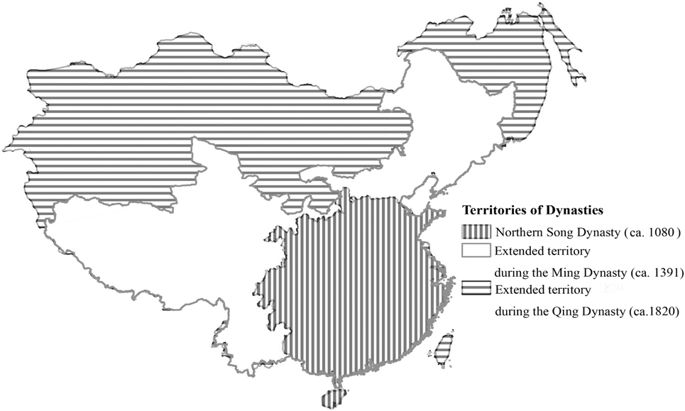
It is important to be clear about how territorial changes have been dealt with in this study, since the Northern Song dynasty covered a smaller area than the Ming dynasty, which in turn covered a smaller area than the Qing dynasty. This is clearly shown in Figure 1, where the Northern Song territory is indicated by the area in the south-east shaded with vertical lines, the Ming territory adds the unshaded areas to the north and west, while the Qing dynasty also includes the areas to the north-east and north-west shaded with horizontal lines. Within each dynasty, however, the territorial coverage has been held constant. Although each dynasty did experience an initial period of territorial expansion, these years are not included in the data set. Thus, the Northern Song is covered for the period 980–1120, consequently avoiding the period of territorial expansion between 960 and 980. Similarly, the territorial expansion of the Ming dynasty between 1368 and 1400 is avoided by restricting the Ming coverage to the period 1400–1620. The Qing dynasty is covered only for the period 1690–1840, thus avoiding the period of territorial expansion between 1644 and 1690. Although the territorial changes were substantial, since the new territories were thinly populated the changes in population and GDP were much smaller. Furthermore, discontinuities in GDP per capita were smaller still. This is similar to the British case used later for comparative purposes, where a change of territory from England to Great Britain in 1700 led to a significant increase in population and GDP but a relatively minor decline in GDP per capita (Broadberry et al. Reference Broadberry, Campbell, Klein and Overton2015).
Territories of The Northern Song, Ming and Qing Dynasties

Detailed data sources are provided in an Online Appendix, and the data set can be downloaded from Broadberry et al. (Reference Broadberry, Guan and Li2018). Inevitability, the results of our calculations must rest on the accuracy of the underlying data, and the previously noted brief survey indicates some areas of potential error. To deal with this uncertainty, we build upon the subjective error margins approach used by Perkins (Reference Perkins1969) for Chinese population and agricultural series. This approach has also been used in other historical national accounting studies for Britain and the Netherlands (Feinstein, Reference Feinstein1972; Feinstein and Thomas Reference Feinstein and Thomas2002; van Zanden and van Leeuwen Reference van Zanden and van Leeuwen2012).
Chinese Economic Growth, 980–1840
Population
We begin with trends in population, which is needed to derive estimates of GDP per capita, the key indicator of overall economic performance in this study. In China, data on the numbers of households and/or individuals assessed for taxation and labor service purposes were collected systematically throughout the period 980–1840. Ho (Reference Ho1959) provides a detailed guide to the nature of the official population data in the Ming and Qing dynasties. It is generally accepted that the officials recorded the number of people accurately, but some adjustments to the official data are necessary because of institutional factors affecting the proportion of the population covered in different periods (Perkins Reference Perkins1969, pp. 193, 203; Ho Reference Ho1959, pp. 3–64). There is broad agreement that the official data for 1381–1382 and 1391 provide an accurate picture of the population for China as a whole, and that the official figures for the late eighteenth century require little adjustment. Between these dates, however, sometimes much larger adjustments are needed to deal with the changing institutional context of data collection (Ho Reference Ho1959, p. 4).Footnote 3 The estimates of Perkins (Reference Perkins1969), Liu and Hwang (Reference Liu and Hwang1979), and Maddison (Reference Maddison1998) build on the insights of Ho (Reference Ho1959) to construct estimates that are sensitive to the changing institutional arrangements to avoid periods of implausibly high population growth rates.
Our estimates for the Ming and Qing dynasties are taken from Maddison (Reference Maddison1998), with some small adjustments described later. The Maddison estimates are close to those of Liu and Hwang (Reference Liu and Hwang1979), who interpolated the data for a number of benchmark years from Perkins (Reference Perkins1969), who provided a correction to the recorded census estimates for the Ming and Qing dynasties that has commanded widespread support. Our minor adjustments during the period 1480–1510 extend the corrections of Maddison (Reference Maddison1998), who thought that Liu and Hwang’s (Reference Liu and Hwang1979) series included some observations with implausibly high decadal population growth rates, but did not consider large unexplained population declines to be a problem. We have dropped Liu and Hwang’s estimates for 1490 and 1500 and log-linearly interpolated between 1480 and 1510, because there is no qualitative historical material to support a sharp drop of more than 15 percent in the population at this time.
For the Northern Song dynasty, our estimates are taken from Wu Songdi (Reference Wu2000), based on official data on the number of households. Wu’s (Reference Wu2000) estimates agree broadly with the figures derived by Kent Deng (Reference Deng2004, p. 43) for the Northern Song dynasty, obtained by multiplying the registered households by a family size of 5.77, the long-term average from years when both household and population data are available. However, Wu (Reference Wu2000, pp. 156–62) suggests a slightly lower family size of 5.4, based on data from local gazetteers and other private sources as well as Song huiyao jigao.
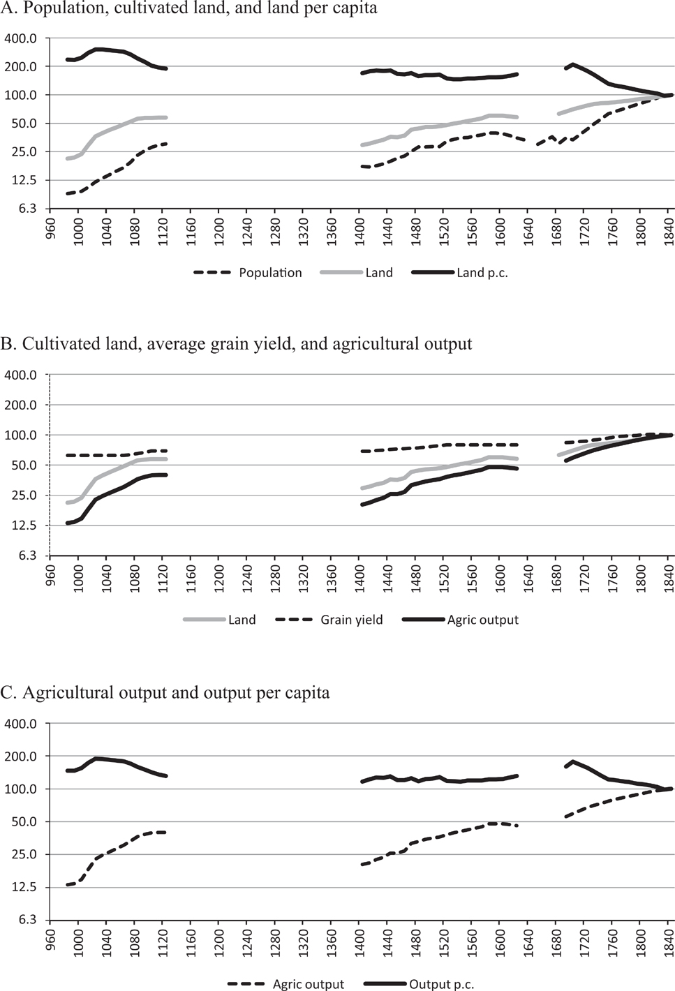
The population data are plotted on a log scale in Figure 2A, and show rapid growth during the Northern Song dynasty at an annual rate of 0.87 percent. Following a substantial decline during the Mongol interlude, population increased during the Ming dynasty, but at a slower rate of 0.32 percent per annum. After another population decline during the next dynastic change, the annual growth rate picked up to 0.70 percent during the Qing dynasty. Although there seems to be a high degree of consensus about the trend of China’s population over this period, the foundational study by Perkins (Reference Perkins1969, p. 216) provides a range of estimates for his benchmark years. This range, based informally on his working knowledge of the data, declines from around ±10 percent in 1393 to ±6 percent in the mid-nineteenth century, but with a greater range in the first half of the seventeenth century associated with the collapse of the Ming dynasty. These margins of error will be used in the reliability assessments and sensitivity analysis.
Chinese Population and Agriculture, 980–1840 (1840 = 100, Log Scale)

Agricultural Output
Agricultural output is estimated mainly from data on the amount of land cultivated and crop yields per unit of land. This section provides an overview of the sources and methods, with more detail provided in Online Appendix A1. The direct output-based approach described in the section on recent developments in historical national accounting has been used by Perkins (Reference Perkins1969) and Liu and Hwang (Reference Liu and Hwang1979) for some parts of the Ming and Qing dynasties, and represents the only feasible quantitative approach for Chinese long-run economic history, due to the absence of reliable wage data needed for the alternative demand-based approach (Álvarez-Nogal and Prados de la Escosura Reference Álvarez-Nogal and de la Escosura2013; Broadberry, Custodis, and Gupta Reference Broadberry, Campbell, Klein and Overton2015). These estimates have been tested and improved by subsequent scholars, leading to important changes during the Qing dynasty in particular, as outlined later.Footnote 4
The starting point for our estimation of output is the cultivated land area. This is derived ultimately from the official data, but also draws upon information obtained from gazetteers and private histories. We use Qi Xia’s (Reference Qi2009) adjustment of the official data for the Northern Song dynasty. For the Ming and Qing dynasties, we use the adjusted figures of Shi Zhihong (Reference Shi2011, Reference Shi2015) and Wang Yeh-chien (Reference Wang2003). The adjustments are necessary because the official data related to tax units rather than the amount of land in arable production (Xu et al. Reference Xu Yi, van Leeuwen and Ni2017, p. 6). The groundwork for the Ming and Qing estimates was laid by Perkins (Reference Perkins1969, pp. 217–40), who drew upon the work of Chinese and Japanese scholars to derive adjustment coefficients for the Ming and early Qing periods. For the period after 1766, Perkins (Reference Perkins1969, pp. 231–40) concluded that the official data had become too far removed from reality, and preferred to work backwards from the 1950s using an index of cultivated land produced by the Agricultural Economics Department of Nanking University and the National Agricultural Research Bureau.
Perkins (Reference Perkins1969, p. 234) demonstrated that the two methods yielded results that were broadly consistent for 1766 and 1873. His estimates have been subsequently improved by Wang (Reference Wang2003) and Shi (Reference Shi2011, Reference Shi2015). For the late Ming and early Qing periods, the adjustment coefficients have been improved by taking account of different rates of tax evasion on private and government fields, and allowing for regional variation (Xu et al. Reference Xu Yi, van Leeuwen and Ni2017, p. 374). For the mid-Qing period, Shi (Reference Shi2011, Reference Shi2015) improves upon Perkins by projecting back from an earlier year in the 1950s and showing that this is consistent with another benchmark for the early 1930s (Xu et al. Reference Xu Yi, van Leeuwen and Ni2017, p. 375). Shi (Reference Shi2015) argues that 1952 is a better benchmark than 1957 because it is distant enough from the preceding wars for the rural economy to have recovered, but not so far from the revolution to have allowed the official data to become too distorted for political reasons (Xu et al. Reference Xu Yi, van Leeuwen and Ni2017, p. 375).
Chao Kang (Reference Kang1986, pp. 80–86) discusses a number of possible reasons apart from tax evasion for under-reporting of the cultivated land area, including incentives provided by emperors to encourage peasants to bring marginal lands into cultivation without being properly registered. The figures provided here have been adjusted for both of these types of underreporting. However, it should be kept in mind that although land data were kept primarily for tax purposes, and that people try to avoid taxes, biases arising from this are unlikely to be too large because people need to register their interest to retain ownership rights (Perkins Reference Perkins1969, p. 217). A more serious worry concerns the lack of a consistent standard measure for the unit of land area, the mu, which varied between regions and over time. Fortunately, however, much effort has been devoted to documenting this variation and the estimates presented here work in terms of a standard mu that is 1/15th of a hectare or 1/6th of an acre (Perkins Reference Perkins1969, pp. 218–21).
Figure 2A plots on a log scale the cultivated land area for the Northern Song, Ming, and Qing dynasties, together with the population series. As we discuss later, because agriculture was the largest sector of the economy, cultivated land per capita plays an important role in determining overall living standards. Although the cultivated land area grew substantially over time, albeit with a major decline between the Northern Song and Ming dynasties, ultimately it did not keep pace with the growth of population so that cultivated land per capita declined over time from a peak of around 9 mu during the Northern Song dynasty to just 3 mu by the late Qing period. Much of this decline occurred during the Qing dynasty, as uncovered by the careful work of Shi (Reference Shi2011, Reference Shi2015).
Given the important role of cultivated land per capita in determining overall living standards, it will be useful to consider the orders of magnitude of potential errors in the estimates. Perkins (Reference Perkins1969, p. 240) again provides a range of estimates for his benchmark years, although as with his population estimates, they reflect subjective judgement rather than formal statistical criteria. His error range for cultivated area declines from just under ±20 percent in 1400 to around ±10 percent by the mid-eighteenth century and under ±5 percent by the late nineteenth century.
Of course, declines in cultivated acreage per capita can be offset by increases in land productivity. Grain yield data largely come from official sources and gazetteers, as set out in Online Appendix A1.2. As noted earlier, there are difficulties of interpretation associated with the variation in the size of a mu over both space and time, but painstaking work by historians to deal with this problem has produced a consensus that grain yields increased over time (Qi Reference Qi2009; Luo Reference Luo1999; Perkins Reference Perkins1969). In addition, some of the grain yield observations are derived from land rent data. There is much evidence to support the contention that the rent was around half the output, so that doubling the rent provides a good measure of crop yields (Perkins, Reference Perkins1969, p. 312). Grain yields are given in jin per mu, where the jin is equal to 1.102 lb. During the Northern Song, wheat yields were stable at 210 jin per mu. With the introduction of high yielding champa rice, husked rice yields increased from 195 to 230 jin per mu, corresponding to an increase in unhusked rice yields from 390 to 460 jin per mu (Qi Reference Qi2009; Wu Reference Wu1985; Ho Reference Ho1956). Guo Songyi (Reference Guo2000) bases his average China-wide yields during the Ming dynasty on a sample covering 37 rice areas in the south and 8 wheat areas in the north, and covering 4 different grades of land (highest, high, middle, and low quality). Average grain yields for wheat and husked rice rose during the Ming dynasty from 220 jin per mu in 1402 to 256 jin per mu by 1626. During the Qing dynasty, Shi (Reference Shi2015) derives average yields for the country as a whole as a weighted average of yields in northern China and southern China broken down into dry farming and paddy farming, with an allowance for multiple cropping. Average grain yields rose from 266 jin per mu in 1685 to 326 jin per mu in 1812. However, this upward trend in grain yields across the three dynasties was insufficient to offset the decline in cultivated land per capita.
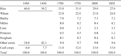
The grain yields used in the calculations are averaged across crops, and reflect the changing distribution of the cultivated land area between crops. These crop distribution data are derived ultimately from official sources, and are shown for benchmark years in Table 1. Rice and wheat were the most important crops during the Northern Song and Ming dynasties, but other crops became more important during the Qing dynasty. In addition to corn and potatoes introduced from the New World, the share of land devoted to cash crops (including sugarcane, hemp, cotton, tobacco, and peanuts) also significantly increased. The cultivated area multiplied by the average grain yield provides a measure of real agricultural output over time. Although separate allowance can be made for cash crops grown on uncultivated land, such as tea and fruit and for livestock, forestry and fishing when calculating the level of agricultural value added in 1840, our key benchmark year for deriving sectoral weights, we lack separate time series information on these subsidiary parts of the agricultural sector.
Distribution of Cultivated Land Area in China by Major Crops 1000–1850 (Percent)

Sources: Wu (Reference Wu1985); Guo (Reference Guo2000); Luo (Reference Luo1999).
Figure 2B plots indices of the cultivated land area and grain yields used to derive the index of agricultural output. Grain yields increased over time, so that agricultural output grew faster than the cultivated land area. However, as Figure 2C makes clear, agricultural output did not increase as fast as population, so that agricultural output per capita declined over time, particularly during the Qing dynasty. Territorial expansion between dynasties was not an important driver of the overall downward trend in agricultural output per capita. Indeed, agricultural output per capita did not decline substantially across either of the dynastic changes in our sample, which might have been expected if territorial expansion had led to growing reliance on more marginal land. Rather, we see that output per capita increased between the later years of the Ming dynasty and the early Qing dynasty. Given the existing literature, there are two noteworthy periods. First, although grain yields per mu did increase significantly during the later years of the Northern Song dynasty, with the introduction of high-yielding champa rice, as noted by Ho (Reference Ho1956), this did not lead to any substantial increase in living standards or output per capita. Indeed, these higher yields were needed just to dampen the negative effects of the decline in cultivated land per capita arising from the rapid population growth of the period. Second, the decline in agricultural output per capita from the eighteenth century is broadly consistent with Philip Huang’s (Reference Huang1985, Reference Huang2002) process of involution. Here again, population growth outstripped the increase in the cultivated land area, and grain yields did not increase sufficiently to offset the fall in land per capita.
Industrial Output
Industry is divided into four main sectors: (1) metals and mining, (2) food processing, (3) textiles and other manufacturing, and (4) building. Our basic approach is to obtain indicators of the volume of output in each main branch of industry and to aggregate these into an index of industrial production using value added weights for the benchmark year of 1840.Footnote 5
The output of the metals and mining sector is tracked using volume data for iron, copper, and salt, taken largely from official sources. This is supplemented by information from gazetteers and private historical sources, particularly where an industry was regionally concentrated. Many economic historians have worked on the original data to provide cross-checks and make up for the shortcomings of individual sources. There have been numerous studies of the iron industry since the strong claims of Robert Hartwell (Reference Hartwell1962) that China produced as much as 150,000 tons of iron in 1078. Subsequent researchers argue that Hartwell seriously overestimated iron production in the Northern Song dynasty and as a result the estimates used here are taken from Liu Sen (Reference Liu1993), obtained by aggregating the annual quantities of iron used for coining and government purchases.Footnote 6 According to Liu, peak iron output in 1078 was around 13,500 tons rather than the 150,000 tons claimed by Hartwell. For the Ming dynasty, the state-run iron industry was based mainly in Zunhua City and the output estimates are based on the official records. The private iron industry is tracked during this period using tax revenue, with the tax rate set at one-fifteenth of output.Footnote 7 For the Qing dynasty, iron industry output is based on regional data for Guangdong, which became the center of the iron mining and metallurgical industry. Li Longqian (Reference Li1979) added data from all other iron-producing provinces to the Guangdong data to estimate the total volume of iron production.
Copper output for the Northern Song dynasty is estimated from official sources. Because copper was used in minting, the industry was strictly regulated by the government, so that few adjustments to the tax quota or ke (er) were needed (Wang Reference Wang2005; Wang Reference Wang1995). Although copper output was much lower during the Ming dynasty, it can be gleaned from official sources for a number of benchmark years. During the Qing dynasty, copper output data are taken from Peng Zeyi (Reference Peng1962), drawing on detailed information for Yunnan province, an important center of copper mining, and more fragmentary information for other regions. For the Northern Song and Qing dynasties, salt output is based mainly on the work of Guo Zhengzhong (Reference Guo1997), who collected data on salt production in different regions and then aggregated the regional estimates to arrive at national salt output. For the Ming dynasty, salt tax data recorded in Ming shilu are supplemented with demand-based estimates using information on consumption per capita.Footnote 8
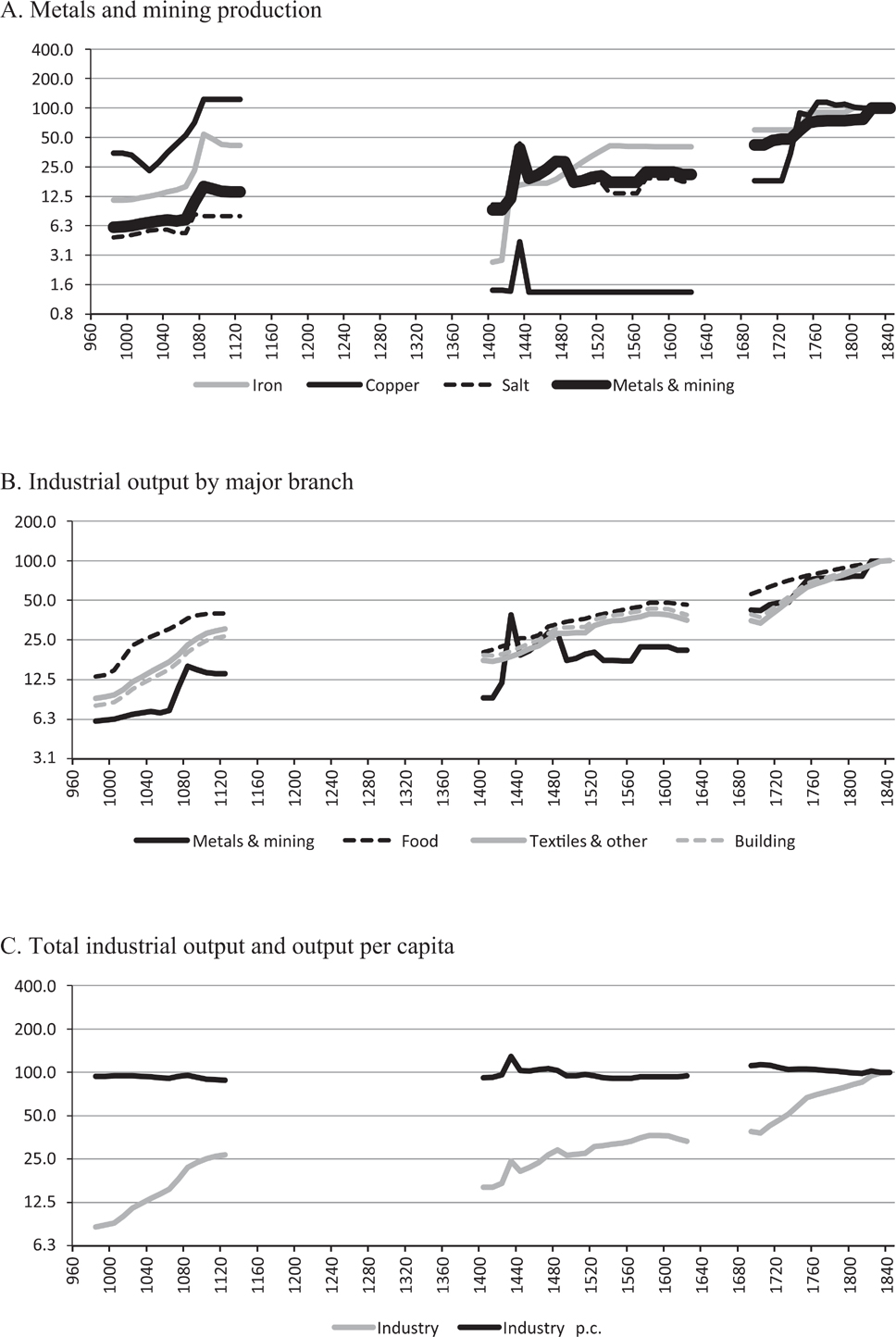
The data in Figure 3A show a good deal of volatility in the output of the iron and copper industries. The boom in these industries during the later years of the Northern Song dynasty is clearly visible, qualitatively consistent (although not quantitatively) with the views of Hartwell (Reference Hartwell1962, Reference Hartwell1966, Reference Hartwell1967). The lower level of activity in these industries during the Ming dynasty was largely the result of developments in the state-owned sector, with a temporary decline in the production of weapons and a more dramatic and long lasting reduction in the minting of coins.Footnote 9 A famous politician and historian of the Ming dynasty, Qiu Jun, estimates that the Ming output of metals was about one to two tenths of the level of the previous dynasty (Daxue yanyi bu, Vol. 29, Shanze Zhili (profits from metals and mining)). The private sector only managed to fully offset these developments during the Qing dynasty, when the government gave up its prohibition of private production, and officials met imperial demand by purchasing metal products in the market. However, although iron and copper have received a great deal of attention in the literature, the value of their output was dwarfed by that of the much larger salt mining industry, which was less volatile.Footnote 10
Chinese Industry, 980–1840 (1840 = 100, Log Scale)

Along with the index of output in the metals and mining branch, Figure 3B presents production indices of the other three main branches of industry. Food processing is assumed to grow in line with agricultural output, following the approach of Broadberry et al. (Reference Broadberry, Campbell, Klein and Overton2015) for England. Building is assumed to grow in line with population, but with an allowance for urbanization, since the growth of towns was associated with more building. This also follows the procedure of Broadberry et al. (Reference Broadberry, Campbell, Klein and Overton2015) in the estimation of English economic growth, 1270–1700. Data on the urbanization rate are taken from Rozman (Reference Rozman1973, pp. 279–83), as presented by Maddison (Reference Maddison1998, p. 35).Footnote 11 Although the building of the Great Wall must have accounted for a significant share of construction activity during the Ming dynasty, most of that construction was completed before 1400. During the period covered by our Ming dataset, 1400–1620, house building accounted for the bulk of construction sector activity. The textile industry, which is taken as representative of other manufacturing, is assumed to grow in line with population, consistent with evidence on cloth consumption per capita (Li Reference Li2005; Xu Reference Xu1992). The food processing, textiles and other manufacturing, and building industries all grew rapidly within the Northern Song, Ming, and Qing dynasties, but with some setback across the dynastic changes.
Figure 3C plots the overall index of industrial production, aggregated using value added weights from Table 2, discussed later. The aggregate index was dominated by the largest sectors, textiles and other manufacturing and building. Food processing grew more slowly in line with agricultural output, while metals and mining showed slightly faster trend growth, but with a greater degree of volatility. Figure 3C also describes our index of Chinese industrial output per capita. Over the long run, industrial production grew at about the same rate as population, so that industrial output per capita exhibits no trend. The boom in the early fifteenth century was due largely to developments in metals and mining and coincides with the famous voyages to the western oceans which demonstrated to the world China’s technological precocity (Maddison Reference Maddison2001, pp. 67–69; Fairbank Reference Fairbank1992, pp. 137–40).
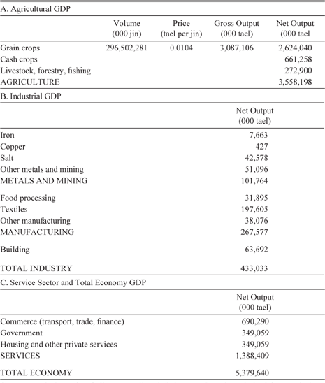
Chinese Current Price GDP in 1840 (000 tael)

Sources: Agriculture: See Online Appendix A3. Industry and services: derived from agriculture using sectoral shares from Zhang (Reference Zhang1987).
Service Sector Output
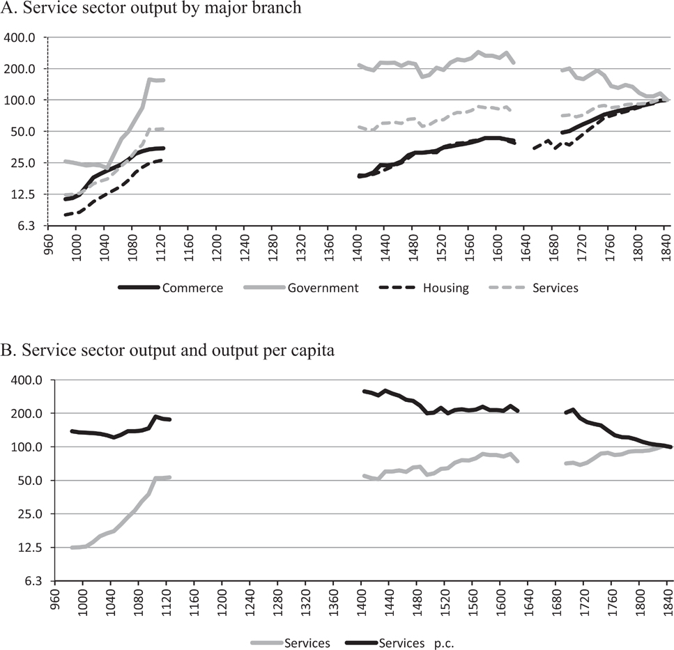
Services have received much less attention from economic historians than have agriculture and industry (Broadberry Reference Broadberry and Gupta2006). Here, the service sector is broken down into three subsectors: (1) commerce, (2) government, and (3) housing and domestic services. Volume indicators are used to construct real output indices for each subsector.Footnote 12
The output of the commercial sector is estimated from data on the volume of agricultural and industrial goods to be distributed. We use 1840 weights of 58 percent for agricultural output and 42 percent for industrial output despite the fact that agriculture was much larger than industry. This is because Wu Hui (Reference Wu1998) finds that only approximately 17 percent of agricultural output was marketed during the Northern Song, Ming, and early Qing dynasties, before rising to 20.7 percent during the later Qing period after 1840, while all industrial output is assumed to be marketed.
For government services, the value of output is calculated from the number of civil servants and soldiers and their salaries, derived from official sources. This yields nominal output, which is deflated by a price index to obtain the real value of government services. The GDP deflator used for this purpose is described in the next section. Following Broadberry et al. (Reference Broadberry, Campbell, Klein and Overton2015), we assumed that housing and domestic service grew in line with population, again with an allowance for urbanization from Rozman (Reference Rozman1973), as for the building sector.
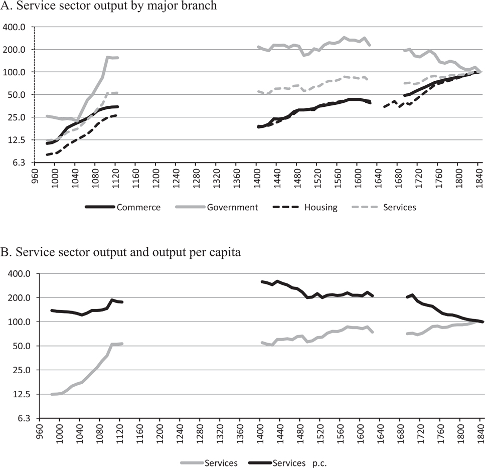
Output indices of the main service sub-sectors are shown in Figure 4A. The most significant long-term trend was the sharp rise in the real size of the government sector during the later years of the Northern Song dynasty, which was maintained during the Ming dynasty, but declined sharply during the Qing dynasty. This appears to be a result of the peak level of government revenue already being reached in nominal terms by the late Northern Song period. As population and the price level both increased above their Northern Song peak levels during the Qing dynasty, the real value of government services on a per capita basis declined sharply. This provides a strong contrast to the rise of the fiscal state in early modern northwest Europe, with growing tax revenues as a share of GDP funding the provision of public goods (Karaman and Pamuk Reference Karaman and Pamuk2010; O’Brien Reference O’Brien2011). As seen in Figure 4B, this pattern of an increase during the Northern Song and a decline during the Qing dynasty is also visible in the overall index of service sector output per capita.
Chinese Services, 980–1840 (1840 = 100, Log Scale)
Gross Domestic Product
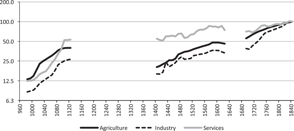
Indices of real output in the agricultural, industrial, and service sectors are plotted together in Figure 5. Over the period as a whole, industry was the fastest growing sector, keeping pace with population, while agriculture grew more slowly. Services grew at about the same rate as agriculture over the long run, but with more of the growth occurring during the Northern Song dynasty. The next step is to combine these sectoral indices into a series of real GDP, which requires a set of value added weights for the benchmark year of 1840. These weights are presented in Table 2. The sectoral shares are taken from the work of Zhang Zhongli (Reference Zhang1987), who estimated Chinese GDP for the 1880s. The absolute level of GDP in 1840 is established by first calculating value added in agriculture for that year, and then applying the shares from the 1880s to calculate nominal value added in industry and services. We argue this is reasonable, given the huge dominance of agriculture in the Chinese economy and the stability of the sectoral shares between the 1880s and 1933, when another estimation of Chinese GDP broken down by sector is available from the work of Wu Baosan and Wang Yusun (Reference Wu and Wang1947).
Chinese Agricultural, Industrial, and Service Sector Output, 980–1840 (1840 = 100, Log Scale)

The level of nominal GDP in agriculture in 1840 is given in Part A of Table 2. We start with the data on crops grown on cultivated land that we used to track the growth of agricultural output over time. The volume of grain output is obtained by multiplying the cultivated land area devoted to grain crops by the average grain yield. This is then multiplied by the average grain price, considering the distribution of crops shown in Table 1. This gives us gross output, which is converted to a net output basis by subtracting the value of agricultural inputs such as seed and fertilizer. Fang Xing (Reference Xing1996) and Luo Yi (Reference Luo1999) suggest that these inputs amounted to 15 percent of gross output during the Qing dynasty, a figure which is also applied to 1933 (Wu and Wang Reference Wu and Wang1947).Footnote 13 The net output of cash crops is set at 25.2 percent of the net output of grain crops, based on the ratio from Zhang (Reference Zhang1987). Zhang (Reference Zhang1987) also yields a ratio of 10.4 percent for the net output of livestock, forestry, and fishing compared to the net output of grain crops.
In Part B of Table 2, the values of net output in the industries that were used in the construction of the index of industrial production are also derived using the sectoral shares from Zhang (Reference Zhang1987), with the 1840 level of agricultural output from Part A of the same table. Within metals and mining, salt was much larger than the iron and copper industries, as noted earlier. Within industry as a whole, metals and mining was larger than food processing and building, but smaller than textiles and other manufacturing (considered together in our production index). Turning to services in Part C of Table 2, levels of net output are again arrived at using the sectoral shares from Zhang (Reference Zhang1987) and taking the 1840 level of net output in agriculture from Part A of Table 2. Commerce was approximately double the size of government services and also housing and other private services. For the total economy, agriculture accounted for 66.1 percent of net output, industry for 8.1 percent, and services for the remaining 25.8 percent.
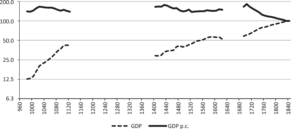
Combining the 1840 weights from Table 2 with the output indices underlying Figures 2 to 5 yields the index of constant price GDP shown in Figure 6. Combined with the population index from Figure 2, this yields our index of GDP per capita, also plotted in Figure 6.Footnote 14 These series will be used in the next section to evaluate the performance of the Chinese economy both domestically across the Northern Song, Ming, and Qing dynasties, and compared with other nations in Europe and Asia.
Chinese Constant Price GDP and GDP per Capita, 980–1840 (1840 = 100)

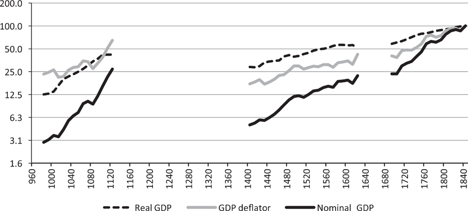
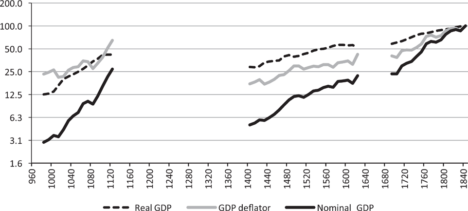
We also need to establish China’s GDP and GDP per capita in nominal as well as in real terms. To do this, we must generate a price index that covers both agricultural and non-agricultural prices. Following the approach of Broadberry, Johann Custodis, and Bishnupriya Gupta (Reference Broadberry, Campbell, Klein and Overton2015) for India, we establish a GDP deflator for China using a grain price index and a cloth price index, with weights of 67 and 33 percent, respectively, in line with the shares of agriculture and non-agriculture in GDP in Table 2. Detailed data sources are provided in Online Appendix A4, and the price index is plotted in Figure 7, together with the index of real GDP from Figure 6. Multiplying real GDP by the GDP deflator yields an index of nominal GDP, which can be used to project back in time from the 1840 benchmark in Table 2 to obtain nominal GDP in taels. Nominal GDP increased from 158 million taels in 980 to 5,380 million taels by 1840. This increase in nominal GDP by a factor of 34.0 was split between an increase in the price level by a factor of 4.3 and a larger increase in real GDP by a factor of 7.9.
Real GDP, The GDP Deflator, and Nominal GDP in China (1840 = 100)
Reliability of the Estimates
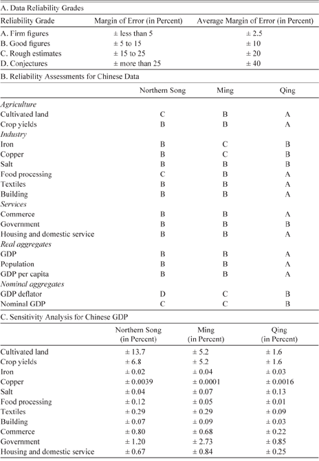
It is worth adding a note of caution, given uncertainties about the accuracy of the underlying data. We have already reported subjective error margins provided by the compilers of some of the most important original series, based on their informed impressions of the reliability of the primary data. To this can be added information gleaned from the range of estimates made by others, as well as the underlying volatility and extent of interpolation in the individual series. Assessments of this type have often been made for official national accounts and were also adopted in Charles Feinstein’s (Reference Feinstein1972, p. 21) historical national accounts for the United Kingdom. The reliability grades, set out in Table 3A, fit quite well with the scale of error margins reported by Perkins (Reference Perkins1969) for the key variables used in our reconstruction of China’s historical national accounts.Footnote 15
Data Reliability Assessments and Sensitivity Analysis

Sources: Reliability assessments based on error margins from Perkins (Reference Perkins1969), comparisons with alternative series produced by other authors and the volatility of the underlying data, as described in the text. Data reliability grades from Feinstein (Reference Feinstein1972, p. 21). Sensitivity analysis shows the percentage increase (decrease) in GDP in response to an increase (decrease) in each series by an amount equal to the average margin of error during each dynasty.
In Table 3B we set out the reliability assessments for all the series used in the construction of the GDP per capita estimates presented in this article. Information on the range and volatility of the underlying series is presented in Online Appendix Table A1, while Table A2 describes the number of observations and methods of interpolation for dealing with missing data. The reliability assessments are based on the error margins from Perkins (Reference Perkins1969) and comparisons with alternative series produced by other authors, together with factors such as the frequency of observations and unexplained volatility in the underlying data.
In Table 3C we conduct sensitivity analysis for Chinese GDP, reporting the percentage increase (decrease) in GDP in response to an increase (decrease) in each component series. Working with a historical study based on Britain, Feinstein and Mark Thomas (Reference Feinstein and Thomas2002, p. 157) follow Chapman (Reference Chapman1953) in assuming that the subjective margins of error are held with 95 percent confidence, so that the average margin of error can be interpreted as two standard errors. Perkins (Reference Perkins1969, p. 216) suggested an 80 percent confidence interval would be more appropriate for the less well documented Chinese case. However, the statistical basis for either of these assumptions is tenuous, so here we eschew a formal statistical interpretation and examine the response of GDP to perturbations of one average margin of error in each series. Chinese GDP is clearly very robust to changes of one average margin of error in most of the component series. Only government during the Northern Song and Ming dynasties and cultivated land and crop yields in all three dynasties affect GDP by more than 1 percent when perturbed by one average error. This is the result of the weight of agriculture and government in the economy rather than the particular unreliability of those series, which are among the best-documented.
The previous exercises highlight where the strengths and weaknesses of the estimates lie. First, the reliability assessments indicate that prices and nominal values are generally less reliable than volume measures, the cultivated land area is less reliable during the Northern Song than during the Qing dynasty, while iron and copper are less reliable during the Ming than in the Northern Song or Qing dynasties. Second, since it is likely that some series will be biased upwards and others downwards, some offsetting errors may be expected in the aggregates derived as the sum of individual series, so long as those series are independently derived (Feinstein and Thomas Reference Feinstein and Thomas2002; Bowley Reference Bowley1911–1912). This explains the B, B, and A grades for GDP during the Northern Song, Ming, and Qing dynasties, respectively, despite some of the component series receiving lower grades. Third, error margins for ratios may also be lower than suggested by the accumulation of error margins for the component series where the errors are positively correlated (Feinstein and Thomas Reference Feinstein and Thomas2002; Bowley Reference Bowley1911–1912). This may be expected to apply to GDP per capita, which is heavily influenced by the ratio of cultivated land to population. Since the population and cultivated land data were collected by the imperial authorities, it is likely that an under-estimate of one was accompanied by an under-estimate rather than an over-estimate of the other.
Chinese Economic Performance
Comparing the Northern Song, Ming, and Qing Dynasties
We now discuss the long-term evolution of the Chinese economy between 980 and 1840 by comparing the growth rate of GDP and the level of GDP per capita during the three dynasties for which data are available. Although China’s territory expanded between the Northern Song and Ming dynasties, and expanded further between the Ming and Qing dynasties, it is nevertheless useful to compare these three dynasties. First, most of the newly extended territory was sparsely populated, and as a result did not have a particularly large effect on the aggregate volume of economic activity. Second, our main concern is with GDP per capita, which was affected even less by territorial changes. The average annual growth rate of real GDP during the Northern Song, Ming, and Qing dynasties was 0.87, 0.27, and 0.36 percent, respectively, although there was also a sharp fall in the level of real GDP (and population) between the end of the Northern Song and the beginning of the Ming dynasties. Real GDP more or less kept pace with population during, as well as between, both dynasties, so that GDP per capita fluctuated without trend but around a high level. During the Qing dynasty, GDP per capita trended strongly downwards at an annual rate of −0.34 percent. As a result, GDP per capita in 1620 was about the same as it had been in 980, but by 1840 had fallen to around 70 percent of its 980 level.
This general pattern of fluctuations without trend around a high level during the Northern Song and Ming dynasties, followed by decline during the Qing dynasty, is broadly consistent with much of the largely qualitative literature on Chinese economic performance over the very long run. The early good performance during the Northern Song and Ming dynasties is most obviously consistent with the work of Mark Elvin (Reference Elvin1973) and his idea of China in a high-level equilibrium trap. The idea of an early peak is also consistent with the view of Chinese science expressed by Joseph Needham (Reference Needham1954), who asked why China was overtaken by the West despite its early scientific successes, such as the development of gunpowder, the magnetic compass, and paper and printing. It also fits with the emphasis of Karl Wittfogel (Reference Wittfogel1957) on the early development of irrigation works, leading to high levels of agricultural productivity, but also a bureaucracy that stifled later development. None of these writers, however, provided any quantitative evidence. Although Hartwell (Reference Hartwell1966) did provide estimates of an impressive level of coke-smelted iron output in the eleventh century, his quantitative evidence was limited to this one sector of the economy.Footnote 16
The idea of a decline in GDP per capita during the Qing dynasty is also most obviously consistent with the work of Huang (Reference Huang1985, Reference Huang2002), who argues that the rapid population expansion at this time led to a growing division of land holdings into ever-smaller plots. Although Huang (Reference Huang1985, pp. 321–27, Reference Huang1990, pp. 340–42) examines the official data on population and cultivated acreage in some districts of North China and the Yangzi Delta, he does not provide systematic quantitative data for China as a whole. However, the decline in the cultivated land per capita, shown in Figure 2A, together with the failure of grain yields to rise sufficiently to offset this over time, shown in Figure 2B, is consistent with Huang’s basic explanation of the decline in living standards. As in our study, recent estimates of Chinese national income produced by Xu et al. (Reference Xu Yi, van Leeuwen and Ni2017) for the period 1661–1933 show a similar percentage decline in GDP per capita during the Qing dynasty.
Note that this pattern of high levels of per capita income during the Northern Song and Ming dynasties, followed by decline during the Qing dynasty differs substantially from the path of Chinese GDP per capita in Maddison (Reference Maddison1998), whose “controlled conjectures” showed an increase from $450 in 1990 international prices to $600 during the Northern Song dynasty, before a long period of stagnation at $600 until the mid-nineteenth century. Our data-based estimates show only a temporary boom in per capita GDP during the Northern Song dynasty rather than Maddison’s (Reference Maddison1998) assumed 33 percent permanent increase. And as noted earlier, our data also indicate a steady decline during the Qing dynasty in contrast to Maddison’s assumed constancy of living standards.
Indeed, this picture of falling living standards during the Qing dynasty is very different from the view of Chinese economic performance painted by California School authors, who see the eighteenth century as a period of economic success for China. On its own terms, the Chinese state would clearly have seen this as a successful period, with new territory and a rapidly expanding population. However, in the modern world which was just emerging during the eighteenth century, economic success was beginning to be measured in terms of rising productivity and living standards. Careful analysis of the cultivated land area and grain yields reveals a decline in per capita food availability, which was not compensated for by an increase in industrial production or service sector output, or by trade in food.
It is worth stating an important implication of rejecting our pattern of decline in GDP per capita during the Qing dynasty. Few would now dispute that China had a low level of GDP per capita by the early nineteenth century. If there was no decline during the Qing period, then this must necessarily mean that China was also very poor during the Ming and Northern Song dynasties, so that any idea of China having once been the richest country in the world would disappear. For, as we shall see later, levels of GDP per capita in Europe were already well above bare bones subsistence levels in the late medieval period.
Comparing China and Britain
It is possible to compare our new GDP per capita estimates for China with the British estimates from Broadberry et al. (Reference Broadberry, Campbell, Klein and Overton2015). However, to do so requires converting the estimates for both countries into a common currency. Following the work of Maddison (Reference Maddison2001, Reference Maddison2010), this is usually done in terms of 1990 international dollars, which Broadberry et al. (Reference Broadberry, Campbell, Klein and Overton2015) do.Footnote 17 If we can establish Chinese GDP per capita as a proportion of British GDP per capita in the mid-nineteenth century, we can thus arrive at a figure for Chinese GDP per capita in 1990 international dollars.Footnote 18
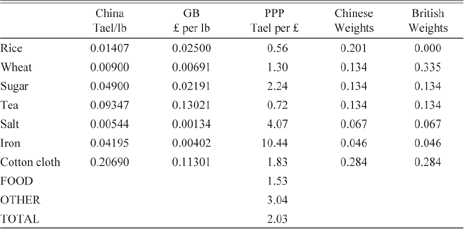
We have data for nominal GDP per capita in 1840 in both countries and prices for a number of important commodities, which can be used to convert the nominal GDP per capita comparison to real terms. Table 4 lays out the 1840 price data for seven commodities which can be grouped into categories covering food and non-food items, with the former divided between unprocessed grain products (wheat and rice) and more processed foods (sugar, tea, and salt). The non-food commodities cover textiles (cotton cloth) and metals (bar iron).Footnote 19 Weights are based on Feinstein (Reference Feinstein1995) and Sara Horrell, Jane Humphries, and Martin Weale (Reference Horrell, Humphries and Weale1994) for Britain, adapted for China to reflect the importance of rice production.Footnote 20 Using British weights, the appropriate price ratio or purchasing power parity (PPP) in 1840 is £1 = 2.11 tael, while at Chinese weights the PPP is £1 = 1.96 tael. Taking the geometric mean of British and Chinese weights, the Fisher index PPP is £1 = 2.03 tael. The nominal exchange rate in 1840, given by the silver weight of the tael compared to the pound sterling was £1 = 3.20 tael. The resulting PPP was substantially below the exchange rate, found also by Allen (Reference Allen2009, pp. 540–43) for the Yangzi Delta in 1820. Note, however, that the PPP was substantially lower for food (£1 = 1.53 tael) than for non-food commodities, where the PPP was close to the exchange rate (£1 = 3.04 tael). This again is a result found by Allen (Reference Allen2009, p. 541) for the Yangzi Delta in 1820 and is explained by the possibility of arbitrage in tradable commodities. Food was less easily tradable than cloth because of the high cost of transporting low value but bulky items which reduced the possibilities of arbitrage.
A China/GB PPP for 1840

Sources and Notes:
GB:
Rice: Beveridge (Reference Beveridge1939, p. 433). The figure of 6s per 12 lb from the Lord Steward’s Department actually refers to 1830.
Wheat: UK Board of Trade (1903, p. 70). The figure of 66s 4d per imperial quarter is taken originally from the London Gazette.
Sugar: UK Board of Trade (1903, p. 162). The average price per cwt unrefined sugar exclusive of duty.
Tea: UK Board of Trade (1903, p. 177). Average price per lb in bond.
Salt: UK Board of Trade (1903, p. 188). Data originally from Greenwich Hospital.
Iron: Mitchell (Reference Mitchell1988, p. 762). English merchant bar iron at Liverpool.
Cotton cloth: Mitchell (Reference Mitchell1988, p. 761). Average value of cotton piece goods exported, converted from yards to lb using 1840 ratio from Robson (Reference Robson1957, p. 331).
Weights: Based on Feinstein (Reference Feinstein1995) for the mid-nineteenth century. Food and non-food items have weights of 0.67 and 0.33, respectively. For the breakdown within food, Feinstein (Reference Feinstein1995) suggests that grain-based products (wheat flour and bread) accounted for around half of expenditure on food. Thus, wheat is given a weight of 0.335 and rice, which was prohibitively expensive, has a weight of zero. The remaining expenditure on food has been allocated across sugar, tea, and salt, with equal weights for sugar and tea and a smaller weight for salt, again broadly consistent with budget studies. Within non-food, the breakdown between cotton and iron is in proportion to the value added in these two industries, from Horrell, Humphries, and Weale (Reference Horrell, Humphries and Weale1994).
China:
Rice: Peng (Reference Peng1965, p. 850).
Wheat: Yiban lu.
Sugar: Fu (Reference Fu1987).
Tea: Yao (Reference Yao1962, vol. 1, p. 582), based on export prices.
Salt: Qingshi gao (Shihuo zhi: Yanfa).
Iron: Kong (Reference Kong1981, pp. 509, 527), wrought iron.
Cotton cloth: Yao (Reference Yao1962, vol. 1, pp. 557, 616), based on export prices.
Weights: The weights are the same as for Britain, apart from an allowance within food for rice, based on the late-Qing ratio between wheat and rice production (30:20). Within non-food, the breakdown between cotton and iron is broadly consistent with the late-Qing shares of value added in textiles and metals production.
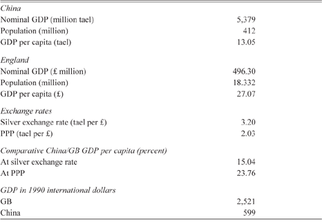
Table 5 provides an estimate of Chinese GDP per capita in 1840 benchmarked on Great Britain. At the silver exchange rate, Chinese GDP per capita was only 15.04 percent of the British level. However, allowing for the lower price level in China in the PPP suggests that Chinese GDP per capita was 23.76 percent of the British level. Taking the 1840 level of British GDP per capita in 1990 international dollars as $2,521 (Broadberry et al. Reference Broadberry, Campbell, Klein and Overton2015) and Chinese GDP per capita in that year as 23.76 percent of the British level, a figure for Chinese GDP per capita in 1990 international dollars is $599. This is close to the figure of $600 suggested by Maddison (Reference Maddison2010) for 1850.
A Benchmark Estimate of China/GB GDP per Capita in 1840

Sources and Notes: Nominal GDP and population from Figures 2 and 7 for China, and from Broadberry et al. (Reference Broadberry, Campbell, Klein and Overton2015) for Britain. Silver exchange rate derived from the silver weight of the tael and pound sterling from von Glahn (Reference von Glahn1996, p. 133) and Craig (Reference Craig1953), respectively. PPP from Table 4. GDP for Britain in 1990 international dollars from Broadberry et al. (Reference Broadberry, Campbell, Klein and Overton2015).
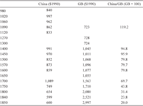
Table 6 presents the GDP per capita series for both China and Britain over the long period 980–1850. These estimates suggest that Northern Song China was richer than Britain at around the time of the Domesday Survey in the late eleventh century. However, per capita incomes then fluctuated without trend in China until the end of the Ming dynasty, while per capita incomes rose in Britain from the mid-fourteenth century, following the mortality crisis of the Black Death. Britain caught up with China by the beginning of the fifteenth century, and then edged ahead. China fell further behind during the Qing dynasty as Chinese per capita incomes declined while incomes started to grow rapidly in Britain from the mid-seventeenth century. By the mid-nineteenth century, Chinese per capita GDP was just 20 percent of the British level.
GDP per Capita Levels in China and Britain (1990 International Dollars)

Sources: GB: Broadberry et al. (Reference Broadberry, Campbell, Klein and Overton2015); Walker (Reference Walker2014). China: Figure 6.
Asia-Europe Comparisons
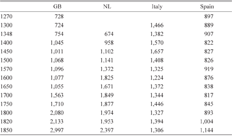
Britain was a relatively poor part of Europe in the eleventh century and a relatively rich part by 1850, as seen in the recent estimates of GDP per capita in Table 7. However, before the Black Death struck in 1348, per capita incomes were substantially higher in Italy and Spain than in Britain and the Netherlands. There then followed a substantial reversal of fortunes between the North Sea area and Mediterranean Europe, so that by 1750, just before the Industrial Revolution, per capita incomes were substantially higher in Britain and the Netherlands than in Italy and Spain. This “Little Divergence” within Europe accompanied the “Great Divergence” between Europe and Asia.
GDP per Capita Levels in Europe (1990 International Dollars)

Sources: Great Britain: Broadberry et al. (Reference Broadberry, Campbell, Klein and Overton2015); Netherlands: van Zanden and van Leeuwen (Reference van Zanden and van Leeuwen2012); Italy: Malanima (Reference Malanima2011); Spain: Álvarez-Nogal and Prados de la Escosura (Reference Álvarez-Nogal and de la Escosura2013).
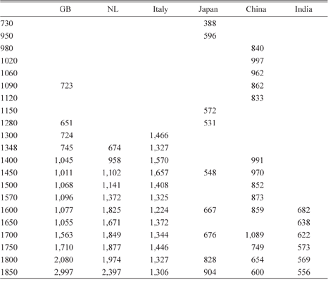
The data in Table 8 also suggest a “Little Divergence” within Asia, with a reversal of fortunes between China and Japan. Japan had very low levels of per capita GDP until 1450, but then experienced episodic growth of the kind seen in Britain and the Netherlands. A phase of positive growth between 1450 and 1600 was followed by a plateau before a second phase of growth from the 1720s. Japan’s more rapid growth after the Meiji Restoration of 1868, which marked the first transition to modern economic growth in Asia, was built on this earlier period of dynamism. This upward trajectory in Japan contrasts with the downward trend in Chinese per capita GDP. Based on these estimates, Japan overtook China during the eighteenth century. India experienced declining GDP per capita from the Mughal peak under Akbar, circa 1600, so that Japan overtook India during the seventeenth century.
GDP per Capita Levels in Europe and Asia (1990 International Dollars)

Sources: GB: Broadberry et al. (Reference Broadberry, Campbell, Klein and Overton2015); Walker (Reference Walker2014); Netherlands: van Zanden and van Leeuwen (Reference van Zanden and van Leeuwen2012); Italy: Malanima (Reference Malanima2011); China: Table 6; Japan: Bassino et al. (Reference Bassino, Broadberry, Fukao and Gupta2017); India: Broadberry, Custodis, and Gupta (Reference Broadberry, Campbell, Klein and Overton2015).
The GDP per capita figures presented here suggest that China was the richest country in the world during the Northern Song dynasty. China was certainly richer than Britain in 1090, sometime after its peak, although Britain had caught up with China by 1400. However, Britain was a relatively poor part of Europe at this time, and comparing China with the richest part of medieval Europe, it is likely that Italy was already ahead by 1300, and perhaps even earlier. By 1500, the Netherlands and Italy were both substantially ahead of China. However, we need to be careful here before concluding that the Great Divergence began in the sixteenth century, since China was much larger than any individual European country, as emphasized by Pomeranz (Reference Pomeranz2000) and Wong (Reference Wong1997). While the GDP per capita gap between the leading North Sea area economies and the whole of China remained small, as it did until the eighteenth century, it is quite possible that a smaller region of China, such as the Yangzi Delta, may still have been on par with the richest parts of Europe.
Sensitivity Analysis
A striking result in this study is the finding of a substantial decline in Chinese GDP per capita during the Qing dynasty, mainly as a result of a large increase in population without an equivalent expansion of the cultivated area or crop yields. This coincided with positive growth of GDP per capita in the leading regions of Europe producing a clear divergence in the eighteenth century, so that the gap between Europe and China became too large to be bridged by regional variation within China. In this section we explore whether it would be possible to restore Pomeranz’s (Reference Pomeranz2000) original finding of a delayed divergence beginning only in the nineteenth century. The answer must surely be no.
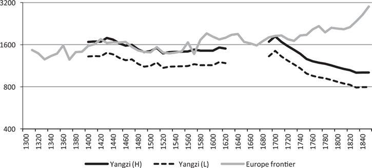
Li Bozhong and Jan Luiten van Zanden (Reference Li and van Zanden2012) have produced a comparison of GDP per capita in the Yangzi Delta and the Netherlands in the early nineteenth century, finding per capita incomes in the Yangzi Delta to be 53.8 percent of the level in the Netherlands in the 1820s. This suggests a per capita GDP figure of $1,050 for the Lower Yangzi, in 1990 international dollars, or about 75 percent higher than in China as a whole. A high estimate for GDP per capita in the Yangzi Delta in earlier years would apply this ratio to our estimates of per capita GDP for China as a whole. This produces our Yangzi (H) series in Figure 8, which also plots the GDP per capita data for the richest part of Europe. The European frontier is based on Italy until the 1540s, followed by the Netherlands until the 1800s and then Great Britain. Although the Netherlands enjoyed a significant lead over the Yangzi Delta in the early seventeenth century, this should be understood as a very small region of Europe, with no other North Sea area economies enjoying a significant advantage over the Yangzi Delta. But once Great Britain, the Netherlands, and Belgium had all forged ahead of the Yangzi Delta during the first half of the eighteenth century, this is too large an area to be ignored. By 1750, Dutch GDP per capita was 49 percent higher than in the Yangzi Delta, rising to an 83 percent lead by 1770. This is well outside the 5 percent error margins for a grade A series such as GDP per capita during the Ming dynasty and indeed even beyond the error margins for a grade B or C series.
GDP per Capita in the Leading Regions of Europe and China, 1300–1850 (1990 International Dollars)

Figure 8 also includes an alternative low estimate of GDP per capita in the Yangzi Delta, shown by the dashed line Yangzi (L). This is derived by rebasing the Yangzi (H) series on an alternative mid-nineteenth century benchmark from Xu et al. (Reference Xu Yi, van Leeuwen and Ni2017). Their figure for China’s GDP per capita in 1850 is obtained by accepting Maddison’s (Reference Maddison2010) estimate for 1933 and projecting backwards using a different series. Instead of our figure of $600 in 1850, this yields an alternative estimate of $472, which is getting quite close to bare bones subsistence of $400, thus providing an effective lower bound.Footnote 21 Note that even with this lower bound series, although western Europe appears to start forging ahead in the sixteenth century, GDP per capita in the Yangzi Delta remains 78 percent of the level of the leading European country as late as 1700, and the first half of the eighteenth century remains a critical juncture.
There are clearly discontinuities in the crucial population and agricultural output series between the Ming and Qing dynasties. Is it possible, therefore, that the decline in agricultural output per capita is a statistical artefact of the Qing data? And if that decline is removed, what are the implications for the Great Divergence debate? On the first point, the break in the population series is actually very short, being confined to the 1640s when the Ming dynasty finally collapsed. However, population was already declining from a peak at the end of the sixteenth century, as China experienced severe pestilence in northern provinces (Cao Reference Shuji2000, pp. 414–43). Southern provinces also suffered population losses during the early years of the Qing dynasty, particularly as a result of the Manchu conquest of the whole of China, but recovery began from the 1650s (Cao Reference Shuji2001, pp. 19–51). As population fell, although there was initially some decline in the total area cultivated, it proceeded more slowly than the decline in population, so that land per capita increased. Agricultural output per capita was thus already rising during the final decades of the Ming dynasty. As population recovered from the 1650s, a decline in land per capita and agricultural output per capita may have been expected, along Malthusian lines. However, because of territorial expansion, land per capita continued to increase, leading to a further significant boost to agricultural output per capita (Shi Reference Shi2015, p. 6). Although the increase of land per capita cannot be distributed across the decades, it is what underlies the increase in agricultural output per capita between 1620 and 1690. In the long run, however, as territorial expansion ceased and population growth continued, land per capita and agricultural output per capita began to decline, as suggested by Huang (Reference Huang1985, Reference Huang1990).
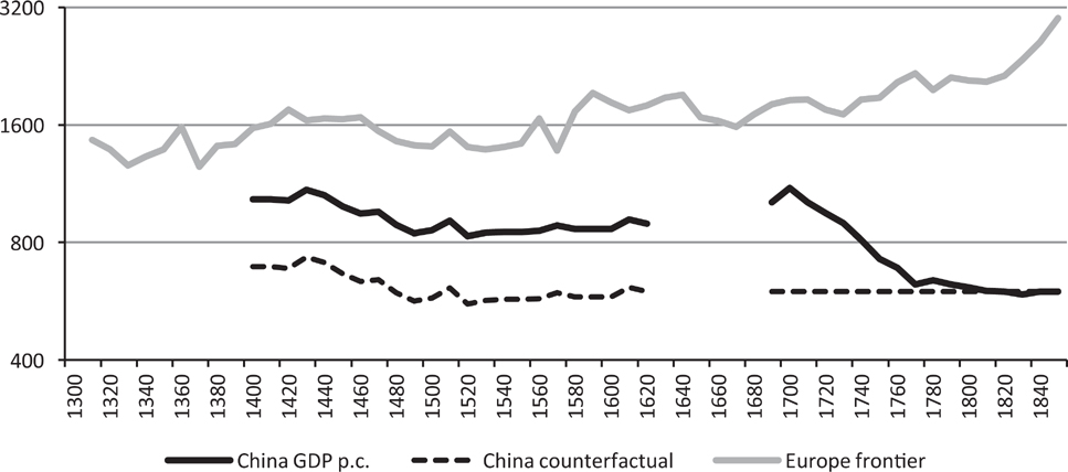
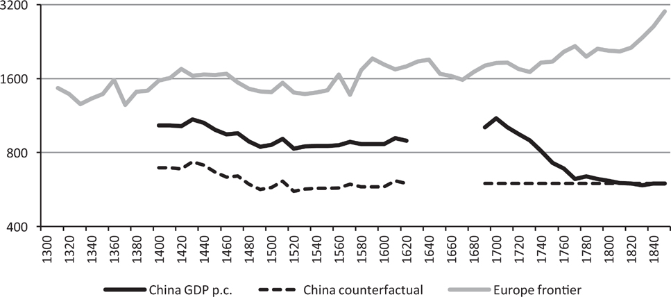
On the second point of what happens if we remove the Qing decline in Chinese per capita GDP, Figure 9 provides another sensitivity test. Here, we investigate the implications of removing the Qing decline, which was driven in turn largely by the decline in agricultural output per capita. This illustrates the key point that if there had been no decline of GDP per capita in China during the Qing dynasty, then China would never have been a rich country, since nobody disputes the fact that it was a very poor country by the mid-nineteenth century. Given the already high levels of per capita GDP in Italy by the fourteenth century, China without a Qing decline would already have been much poorer than Europe in the medieval period, so that the idea of a late Great Divergence would not even arise.
Counterfactual GDP per Capita in China Compared with the Frontier in Europe, 1300–1850 (1990 International Dollars)
It is reassuring that the historical national accounting evidence suggests the first half of the eighteenth century as the point in time when the gap between Europe and Asia became too large to ignore, since this seems to be the new consensus that is emerging from both California School authors such as Pomeranz (Reference Pomeranz2011) and from economic historians using other quantitative indicators such as real wages and urbanization rates (Broadberry and Gupta Reference Broadberry2006; Allen et al. Reference Allen, Bassino, Ma and Moll-Murata2011).
Conclusions
This article provides estimates of Chinese GDP and relative standing in the world constructed from the output side between 980 and 1840, covering the Northern Song, Ming, and Qing dynasties. These GDP estimates are combined with population data to track the path of GDP per capita. China’s GDP per capita fluctuated around a high level during the Northern Song and Ming dynasties, before trending downwards during the Qing dynasty, falling to around 70 percent of its 980 level by 1840.
From an international perspective, Northern Song China was richer than Domesday Britain in 1090, but Britain had caught up with China by the fifteenth century. Although China had the highest standard of living in the world during the Northern Song dynasty, Italy had already forged ahead by 1300. At this point, however, and even until the eighteenth century, it is quite possible that a relatively rich Chinese region such as the Yangzi Delta was on par with the most developed parts of Europe. But Chinese GDP per capita declined sharply during the Qing dynasty, just when parts of northwest Europe made the transition to modern economic growth, so that by the middle of the eighteenth century, the gap between China and the most developed parts of Europe was too large to be bridged by any discussion of regional variation within China. Since China was still the richest Asian country at this time, it is therefore likely that western Europe was significantly ahead of Asia not just by the early nineteenth century, but already by the mid-eighteenth century, before the Industrial Revolution. The Great Divergence thus began earlier than originally suggested by the California School, but later than implied by older Eurocentric writers.
Main Data Series (1840 = 100)