





1. Introduction
Birefringent strands (Harlen, Rallison & Chilcott Reference Harlen, Rallison and Chilcott1990) are localized regions of large strain and stress in viscoelastic flows of polymer solutions. At the molecular level, they correspond to polymers that are highly stretched and tend to align in a thin region that is optically anisotropic. Birefringent strands have been observed in a variety of systems (Mackley Reference Mackley1978; Keller & Odell Reference Keller and Odell1985), including roll mills (Crowley et al. Reference Crowley, Frank, Mackley and Stephenson1976; Farrell & Keller Reference Farrell and Keller1978; Fuller & Leal Reference Fuller and Leal1980; Lee et al. Reference Lee, Kapur, Gaskell, Savage and Homsy2002), opposed jets (Müller, Odell & Keller Reference Müller, Odell and Keller1988; Odell, Müller & Keller Reference Odell, Müller and Keller1988), cross-slot devices (Scrivener et al. Reference Scrivener, Berner, Cressely, Hocquart, Sellin and Vlachos1979; Miles & Keller Reference Miles and Keller1980; Odell & Carrington Reference Odell and Carrington2006; Haward & McKinley Reference Haward and McKinley2013; Sousa et al. Reference Sousa, Pinho, Oliveira and Alves2015), flows around cylinders (Haward & McKinley Reference Haward and McKinley2013; Sun & Huang Reference Sun and Huang2016; Haward et al. Reference Haward, Toda-Peters and Shen2018; Hopkins et al. Reference Hopkins, Haward and Shen2020) and flows around spheres (Haward & Odell Reference Haward and Odell2004). Examples of flow-induced birefringence in the case of a cross-slot device and the flow around one and two cylinders are shown in figure 1.
Examples of experimental observations of the formation of birefringent strands in the literature, with (a,d,f) cases with one cylinder; (c,e,g) cases with two cylinders; and (b) a cross-slot device. In (f,h,g,i), the results correspond to two different regimes of flow with (f,g) steady symmetric and (h,i) steady asymmetric. Panels (a,c) are reproduced from Haward, Toda-Peters & Shen (Reference Haward, Toda-Peters and Shen2018) with permission. Panel (b) is reproduced from Haward & McKinley (Reference Haward and McKinley2013) with permission. Panels (d,e) are reproduced from Sun & Huang (Reference Sun and Huang2016) with permission. Panels (f–i) are reproduced from Hopkins, Haward & Shen (Reference Hopkins, Haward and Shen2020) with permission. In all panels, birefringence is characterized by the retardation,  $R(\text {nm})$, between two optical paths, which stems from differences in refractive index due to polymer molecules. This local change in the optical property of the polymer solution is also a proxy for visualizing stress as it can be linked to the local principal stress difference through the stress–optic law, which states that there is a linear relationship between
 $R$ and the difference in principal stresses.

Geometries with a cylinder are often used as model systems to study the fundamental fluid mechanics of viscoelastic flow past solid obstacles – in experiments (François et al. Reference François, Lasne, Amarouchene, Lounis and Kellay2008; Shi & Christopher Reference Shi and Christopher2016; Varshney & Steinberg Reference Varshney and Steinberg2017; Qin et al. Reference Qin, Salipante, Hudson and Arratia2019b), numerical approaches (Chilcott & Rallison Reference Chilcott and Rallison1988; Liu et al. Reference Liu, Bornside, Armstrong and Brown1998; Fan, Yang & Tanner Reference Fan, Yang and Tanner2005; Wapperom & Renardy Reference Wapperom and Renardy2005; Bajaj, Pasquali & Prakash Reference Bajaj, Pasquali and Prakash2008) and theoretical analyses (Renardy Reference Renardy1997; Becherer, van Saarloos & Morozov Reference Becherer, van Saarloos and Morozov2009). Flow around a cylinder leads to the formation of a birefringent strand in the wake. The strand develops close to stagnation points, where elongation is strong and the residence time is long compared with the relaxation time of the polymer (Harlen et al. Reference Harlen, Rallison and Chilcott1990), and is then transported with a competition between advection and relaxation. Continuum representations of the viscoelastic flow, in particular Oldroyd-B and finitely extensible nonlinear elastic (FENE)-type models, capture the formation of the strands through a two-way coupling between a polymeric stress tensor,  $\boldsymbol{\mathsf{\tau}}_{p}$, in the momentum balance and a separate transport equation for its components.
The problem can be simplified by considering a one-way coupling with no feedback of the polymeric stress upon the velocity field, for instance in a limit of extreme dilution. The velocity field is calculated in the Newtonian limit and then used for the transport of the polymeric stress. This approach has made it possible to determine the structure of the stress field and its scalings near a curved boundary (Renardy Reference Renardy1997), around a cylinder and in its wake (Renardy Reference Renardy2000) or near a flat wall (Becherer et al. Reference Becherer, van Saarloos and Morozov2009; Van Gorder, Vajravelu & Akyildiz Reference Van Gorder, Vajravelu and Akyildiz2009). On the other hand, the feedback of the strand upon the flow has been described through approaches such as the birefringent strand technique, which treats the strand of extended polymers as a line distribution of forces surrounded by a Newtonian fluid (Rallison & Hinch Reference Rallison and Hinch1988; Harlen et al. Reference Harlen, Rallison and Chilcott1990). This force, exerted by the polymers upon the fluid, leads to a jump in shear rate across the strand and to a decrease of the velocity in the wake of the cylinder (Harlen et al. Reference Harlen, Rallison and Chilcott1990). This method was also used in Harlen (Reference Harlen1990) for the flow past a falling sphere, in Harlen, Hinch & Rallison (Reference Harlen, Hinch and Rallison1992) to study the case of an opposed jet, in Lee et al. (Reference Lee, Kapur, Gaskell, Savage and Homsy2002) for a co-rotating two-roll mill and in Málaga & Rallison (Reference Málaga and Rallison2007) for rising bubbles.
Configurations with more than one cylinder have also been recently considered to unravel interaction mechanisms. For instance, Haward et al. (Reference Haward, Toda-Peters and Shen2018) studied the case of two cylinders aligned with the flow using microfluidics. They show that the strand formed in the wake of the first cylinder can interact with the second cylinder, encapsulate it completely and even create a stagnation zone between the two cylinders. Hopkins, Haward & Shen (Reference Hopkins, Haward and Shen2021) considered the case of two cylinders in a confined microfluidic channel – with the line segment joining the centres of the cylinders being orthogonal to the flow direction – and studied the flow as a function of the gap between the cylinders. For small gaps, the flow is ‘divergent’, with the flow rate between the cylinders being smaller than in the Newtonian case. For large gaps, on the contrary, the flow converges with the flow rate between the cylinders being larger than in the Newtonian case. A rupture of symmetry can occur, which was also observed in the case of a single cylinder (see figure 1f,h). This phenomenon is linked to the shear-thinning rheology of the fluid (Haward et al. Reference Haward, Kitajima, Toda-Peters, Takahashi and Shen2019; Haward, Hopkins & Shen Reference Haward, Hopkins and Shen2020; Haward et al. Reference Haward, Hopkins, Varchanis and Shen2021b; Varchanis et al. Reference Varchanis, Hopkins, Shen, Tsamopoulos and Haward2020) and is hypothesized to stem from a positive feedback mechanism involving the strand (Haward et al. Reference Haward, Hopkins, Varchanis and Shen2021b). Khan & Sasmal (Reference Khan and Sasmal2021) recovered these results and showed a change of curvature sign in the convergent and divergent cases. This observation, along with the known effect of a strand in slowing down the flow in the wake of a single cylinder, suggests that strands may play a central role in controlling the relative flow through the different parts of the geometry and the transition mechanisms.
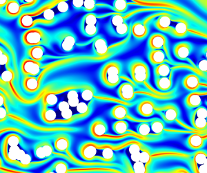
In porous media, little is known about the interaction between the strands, the flow and the geometrical structure. De et al. (Reference De, Kuipers, Peters and Padding2017a) observed numerically the formation of strands in steady flows through random arrays of cylinders and the concomitant appearance of preferential flow paths. To illustrate such effects, we show in figure 2 some results of our steady state simulations for an incompressible Oldroyd-B fluid in a two-dimensional (2-D) geometry with biperiodic conditions and a body force oriented from left to right (see § 5). The strands exhibit surprisingly rich behaviours that have yet to be understood. In some regions, they completely encapsulate large regions containing some fluid and several cylinders. In other regions, they form channel-like structures that seem to drive the flow paths through the structure. This raises many questions about these strands including how they modify the flow, how they interact with solid obstacles and with each other or what their effect is on larger scales. For instance, could these strands be involved in the increase of flow resistance through porous structures – a phenomenon reported in numerous studies (Marshall & Metzner Reference Marshall and Metzner1967; James & McLaren Reference James and McLaren1975; Durst, Haas & Kaczmar Reference Durst, Haas and Kaczmar1981; Kauser et al. Reference Kauser, Dos Santos, Delgado, Müller and Sáez1999)? Although a variety of hypotheses have been formulated, such as the effect of extensional viscosity of the fluids (Durst, Haas & Interthal Reference Durst, Haas and Interthal1987; Chmielewski & Jayaraman Reference Chmielewski and Jayaraman1992; Khomami & Moreno Reference Khomami and Moreno1997; Rothstein & McKinley Reference Rothstein and McKinley2001; Zamani et al. Reference Zamani, Bondino, Kaufmann and Skauge2015; Skauge et al. Reference Skauge, Zamani, Gausdal Jacobsen, Shaker Shiran, Al-Shakry and Skauge2018) or elastic turbulence (Galindo-Rosales et al. Reference Galindo-Rosales, Campo-Deano, Pinho, Van Bokhorst, Hamersma, Oliveira and Alves2012; Clarke et al. Reference Clarke, Howe, Mitchell, Staniland and Hawkes2016; Machado et al. Reference Machado, Bodiguel, Beaumont, Clisson and Colin2016; Kawale et al. Reference Kawale, Marques, Zitha, Kreutzer, Rossen and Boukany2017; Qin et al. Reference Qin, Salipante, Hudson and Arratia2019a; Browne & Datta Reference Browne and Datta2021), a detailed picture of the problem that clearly links pore-scale physics with larger scales is still lacking.
Example simulations of the flow of an Oldroyd-B fluid through an array of cylinders in the case with a Weissenberg number  ${\simeq }5$ and
 $\beta =1$ (see § 2.1 for definitions). Plots of (a) the trace of the conformation tensor
 ${\rm tr}(\boldsymbol{\mathsf{c}})$, which represents the stretching of the polymer chains, and (b) velocity magnitude
 $\Vert \,\boldsymbol {u}\Vert$.

In this work, our goal is to study the formation of strands past obstacles and in porous structures to understand how they modify the flow, how they interact with each other and how they interact with the solid structure. With this fundamental understanding at the pore scale, we also aim at providing a link with the macro-scale through energetic considerations. Our numerical approach is presented in § 2 and is based upon the Oldroyd-B model (§ 2.1), which has proven very useful in describing Boger-type viscoelastic fluids with constant viscosity in simple shear flow (James Reference James2009; Shaqfeh & Khomami Reference Shaqfeh and Khomami2021). Viscoelastic fluids give rise to rich physics even without inertial effects (Larson Reference Larson2000) so that we focus here on steady incompressible flow in the creeping limit. We use simulations based on a recently developed high performance computing (HPC) code (Mokhtari et al. Reference Mokhtari, Davit, Latché and Quintard2021) that is summarized in § 2.2. We cannot start directly with porous structures since, as illustrated in figure 2, the fields are complex and difficult to interpret. Rather, our strategy consists of progressively increasing the complexity of the problem, starting with a single cylinder (§ 3). We detail the fundamental mechanisms that generate the strand, describe its behaviour and quantify important properties, in particular its length and its effect upon the flow. We then study cases with two cylinders (§ 4) either aligned with the flow or with the line segment joining the centres of the cylinders that is orthogonal to the flow direction, outlining strand/cylinder and strand/strand interactions and quantifying their effect upon the flow. Finally, we get back to more complex porous media consisting of arrays of cylinders (§ 5) and compute pore-scale and Darcy-scale quantities, in particular the resistance to flow for a range of Weissenberg numbers and ratios of polymer to solvent viscosities.
2. Numerical approach
2.1. Governing equations
We consider the Oldroyd-B model for an incompressible fluid in the creeping flow limit. Momentum and continuity equations read
 \begin{equation} \left. \begin{gathered} -\boldsymbol{\nabla} \mathfrak{p}+\eta_{s}\boldsymbol{\nabla} \boldsymbol{\cdot}\left(\boldsymbol{\nabla} \boldsymbol{\mathfrak{u}}+\left(\boldsymbol{\nabla} \boldsymbol{\mathfrak{u}}\right)^{\mathrm{T}}\right)+\boldsymbol{\nabla} \boldsymbol{\cdot}\boldsymbol{\mathsf{\tau}}_{p}+\boldsymbol{\mathfrak{F}} =0,\\ \boldsymbol{\nabla} \boldsymbol{\cdot}\boldsymbol{\mathfrak{u}} =0, \end{gathered} \right\} \end{equation}
where  $\eta _{s}$ is the solvent viscosity,
 $\boldsymbol {\mathfrak {u}}$ the fluid velocity,
 $\mathfrak {p}$ the pressure,
 $\boldsymbol {\mathfrak {F}}$ is a body force acting on the fluid,
 $\boldsymbol{\mathsf{\tau}}_{p}$ is the polymeric stress, and superscript T denotes the transpose operator. In the Oldroyd-B model,
 $\boldsymbol{\mathsf{\tau}}_{p}$ is proportional to the deviation of the conformation tensor from its equilibrium state
 \begin{equation} \boldsymbol{\mathsf{\tau}}_{p}={\eta_{p}}/{\lambda}\left(\boldsymbol{\mathsf{c}}-\boldsymbol{\mathsf{I}}\right), \end{equation}
with  $\eta _{p}$ a viscosity associated with the polymers,
 $\lambda$ a relaxation time,
 $\boldsymbol{\mathsf{c}}$ the conformation tensor and
 $\boldsymbol{\mathsf{I}}$ the identity matrix. The constitutive equation for the evolution of the conformation tensor is given by
 \begin{equation} \partial_{t}\boldsymbol{\mathsf{c}}+\left(\boldsymbol{\mathfrak{u}}\boldsymbol{\cdot}\boldsymbol{\nabla} \right)\boldsymbol{\mathsf{c}}=\boldsymbol{\nabla} \boldsymbol{\mathfrak{u}}\,\boldsymbol{\mathsf{c}}+\boldsymbol{\mathsf{c}}\left(\boldsymbol{\nabla} \boldsymbol{\mathfrak{u}}\right)^{\mathrm{T}}-\frac{1}{\lambda}\left(\boldsymbol{\mathsf{c}}-\boldsymbol{\mathsf{I}}\right). \end{equation}
Non-dimensionalizing space by a length scale  $R$ and time by
 ${R}/{U}$, where
 $U$ is a reference velocity, we obtain the following dimensionless version of the equations:
 \begin{gather} -\boldsymbol{\nabla} p+\boldsymbol{\nabla} \boldsymbol{\cdot}\left(\boldsymbol{\nabla} \boldsymbol{u}+\left(\boldsymbol{\nabla} \boldsymbol{u}\right)^{\mathrm{T}}\right)+\frac{\beta}{Wi}\boldsymbol{\nabla} \boldsymbol{\cdot}\boldsymbol{\mathsf{c}}+\boldsymbol{F} =0, \end{gather}
 \begin{gather}\boldsymbol{\nabla} \boldsymbol{\cdot}\boldsymbol{u} =0, \end{gather}
 \begin{gather}\partial_{t}\boldsymbol{\mathsf{c}}+\left(\boldsymbol{u}\boldsymbol{\cdot}\boldsymbol{\nabla} \right)\boldsymbol{\mathsf{c}} =\boldsymbol{\nabla} \boldsymbol{u}\,\boldsymbol{\mathsf{c}}+\boldsymbol{\mathsf{c}}\left(\boldsymbol{\nabla} \boldsymbol{u}\right)^{\mathrm{T}}-\frac{1}{Wi}\left(\boldsymbol{\mathsf{c}}-\boldsymbol{\mathsf{I}}\right), \end{gather}
where  $\beta ={\eta _{p}}/{\eta _{s}}$ is a viscosity ratio and
 $Wi={\lambda U}/{R}$ the Weissenberg number. This system of equations must be complemented by suitable boundary and initial conditions for the velocity and the conformation tensor. For initial conditions, we will consider uniform fields in the form
 $\boldsymbol {u}=\boldsymbol {u}_{0}$ and
 $\boldsymbol{\mathsf{c}}=\boldsymbol{\mathsf{c}}_{0}$, where
 $\boldsymbol{\mathsf{c}}_{0}$ is a symmetric positive definite tensor. Unless otherwise stated, we impose
 $\boldsymbol {u}_{0}=\boldsymbol {0}$ and
 $\boldsymbol{\mathsf{c}}_{0}=\boldsymbol{\mathsf{I}}$.
Since the Oldroyd-B model has a clear physical connection to polymer chains, involves relatively few parameters and is one of the simplest models that is capable of capturing some of the complex features of viscoelastic flows, it is a natural starting point for many studies of dilute polymer solutions (Shaqfeh & Khomami Reference Shaqfeh and Khomami2021). It has some well-known shortcomings, such as the infinite extensibility of polymer chains in elongation – an issue that can make numerical approximations and convergence difficult, for example when trying to precisely capture the stress profile in the strand in the wake of a single cylinder (Hulsen, Fattal & Kupferman Reference Hulsen, Fattal and Kupferman2005; Damanik et al. Reference Damanik, Hron, Ouazzi and Turek2010; Mokhtari et al. Reference Mokhtari, Davit, Latché and Quintard2021). Extensions of this model that are based upon a non-affine relation between the stress and the conformation tensor can be used to overcome this particular issue. This includes the FENE-P model (Bird, Dotson & Johnson Reference Bird, Dotson and Johnson1980),
 \begin{equation} \boldsymbol{\mathsf{\tau}}_{p}=\frac{\eta_{p}}{\lambda}\left(\frac{b}{b-{\rm tr}(\boldsymbol{\mathsf{c}})}\boldsymbol{\mathsf{c}}-\frac{b}{b-{\rm tr}(\boldsymbol{\mathsf{I}})}\boldsymbol{\mathsf{I}}\right), \end{equation}
where  $b>d$ with
 $d$ the spatial dimension. This model imposes a bound upon the stretching of the polymers,
 $\textrm {tr}(\boldsymbol{\mathsf{c}})< b$. Contrary to the Oldroyd-B model, it does not describe a Boger fluid (Herrchen & Öttinger Reference Herrchen and Öttinger1997) but rather couples elastic effects with shear thinning. This can be useful to reproduce experimental observations but may also be a problem when actually trying to decouple the different mechanisms to study the fundamentals of viscoelastic flows. A closely related formulation is the FENE-CR model (Chilcott & Rallison Reference Chilcott and Rallison1988) with
 \begin{equation} \boldsymbol{\mathsf{\tau}}_{p}=\frac{\eta_{p}}{\lambda}\frac{b}{b-{\rm tr}(\boldsymbol{\mathsf{c}})}\left(\boldsymbol{\mathsf{c}}-\boldsymbol{\mathsf{I}}\right). \end{equation}
This model also imposes a bound upon the stretching of the polymers,  $\textrm {tr}(\boldsymbol{\mathsf{c}})< b$, so that mesh convergence is easier than for the Oldroyd-B model (Kim et al. Reference Kim, Kim, Chung, Ahn and Lee2005; Mokhtari et al. Reference Mokhtari, Davit, Latché and Quintard2021). It is similar to the FENE-P model in elongational flow (Chilcott & Rallison Reference Chilcott and Rallison1988; Keunings Reference Keunings1997) and similar to the Oldroyd-B in shear flows. In particular, it is a description of a Boger fluid (Herrchen & Öttinger Reference Herrchen and Öttinger1997) with constant shear viscosity, thus making it possible to separate elastic effects from shear thinning. Compared with the Oldroyd-B, FENE-type models have the disadvantage of introducing another source of nonlinearity to the equations, which must be dealt with carefully in numerical simulations, and of involving an additional parameter
 $b$ that is not strictly necessary to describe interactions between birefringent strands and flow. The rationale behind our choice of using the Oldroyd-B model is that we want to understand some of the fundamental aspects of viscoelastic flows past obstacles, while keeping the model as minimal as possible. This approach is supported by our own comparisons between the FENE-CR and Oldroyd-B models in Mokhtari et al. (Reference Mokhtari, Davit, Latché and Quintard2021), showing that the backbone of the stress fields remains the same for both models.
A schematic 2-D geometry is represented in figure 3, along with the two types of boundary conditions that we will use in this work. The characteristic length scale,  $R$, for the non-dimensionalization will be the radius of the cylinders. Boundary conditions on the surface of the cylinder are no-slip and no-penetration boundary conditions,
 $\boldsymbol {u}=\boldsymbol {0}$. Periodic boundary conditions are used for the top/bottom boundaries and two types of boundary conditions will be considered for the left/right boundaries, with either
(i) inlet/outlet boundary conditions. In this case, Dirichlet conditions
 $\boldsymbol {\mathfrak {u}}=\boldsymbol {\mathfrak {u}}_{in}$ and $\boldsymbol{\mathsf{c}}=\boldsymbol{\mathsf{I}}$ are imposed for both the velocity and the conformation tensor at the inlet. The reference velocity will then be the Euclidean norm of the inlet velocity, $U=\Vert \boldsymbol {\mathfrak {u}}_{in}\Vert$. At the outlet, the fluid is supposed to obey a Neumann boundary condition, with an external force normal to the boundary
(2.9)where\begin{equation} \left({-}p\boldsymbol{\mathsf{I}}+\boldsymbol{\nabla} \boldsymbol{u}+\left(\boldsymbol{\nabla} \boldsymbol{u}\right)^{\mathrm{T}}+\frac{\beta}{Wi}\boldsymbol{\mathsf{c}}\right)\boldsymbol{n}_{ext}={-}p_{ext}\boldsymbol{n}_{ext},\end{equation}$\boldsymbol {n}_{ext}=\boldsymbol {e}_{x}$ is the normal vector, $\boldsymbol {e}_{x}$ being the first vector of the canonical basis of $\mathbb {R}^{2}$. The external pressure $p_{ext}$ is fixed to zero. When these boundary conditions are used, we systematically have $\boldsymbol {F}=\boldsymbol {0}$;
(ii) periodic boundary conditions, leading to biperiodicity. The flow is then imposed through a uniform body force
$\boldsymbol {F}=F\boldsymbol {e}_{x}$. The reference velocity for non-dimensionalization is determined a posteriori because the velocity is not imposed, but rather results from the body force. This velocity is calculated as the Euclidean norm of the average velocity, $U=\Vert \langle \boldsymbol {\mathfrak {u}}\rangle \Vert$ where the averaging operator is defined by
(2.10)with\begin{equation} \left\langle \bullet\right\rangle =\frac{1}{\left|\varOmega\right|}\int_{\varOmega}\mathcal{\bullet}\,{\rm d}S \end{equation}$\varOmega$ the fluid part of the domain. Note that, with this definition, the average velocity $\langle \boldsymbol {u}\rangle$ is the intrinsic velocity of the fluid and not the Darcy velocity. For cases with one or two cylinders, the porosity is close to 1 so that the values of intrinsic and Darcy velocities are very similar. For arrays of cylinders, intrinsic and Darcy velocities are significantly different.This periodic boundary condition is useful in two cases: flows through a lattice of cylinders and obstacles in a channel. For the cylinder lattice, periodic boundary conditions are a rather natural choice to mimic flow through a porous medium (Sanchez-Palencia Reference Sanchez-Palencia1982; Whitaker Reference Whitaker1986). For the channel case, this is essentially a numerical trick to avoid dealing with the entrance length and to simplify boundary conditions in calculating different orders of asymptotic developments. To avoid interactions between periodicity and strand formation, we make sure that the length of the channel is long enough for relaxation to occur. For example, in the case of a single cylinder, a strand reaching the outlet will be reintroduced at the inlet and may interfere with the flow if the channel is too short. To prevent this, the channel must be long enough so that the conformation tensor has enough time to relax to equilibrium and the strand disappears before reaching the outlet.


Typical geometry with boundary conditions. The boundary conditions are top–bottom periodicity and  $\boldsymbol {u}=(0,0)^{\mathrm {T}}$ on the cylinder. Two types of boundary conditions are used for left- and right-hand sides, either (a) an inlet condition on the left-hand side,
 $\boldsymbol {u}=(1,0)^{\mathrm {T}}$ and
 $\boldsymbol{\mathsf{c}}=\boldsymbol{\mathsf{I}}$, and an outlet condition on the right-hand side,
 $p_{ext}=0$ (see (2.9)), or (b) periodic boundary conditions with the flow generated through a body force
 $\boldsymbol {F}$. (a) Inlet/outlet. (b) Biperiodic.

2.2. Numerical method
To solve this problem, we have developed a novel approach that is detailed and validated against two benchmarks (lid-driven cavity and confined cylinder) in Mokhtari et al. (Reference Mokhtari, Davit, Latché and Quintard2021). Here, we simply summarize the numerical scheme, which implements a fractional step approach. First, the unstationary Stokes system (i.e. mass and momentum balance equations) is decoupled from the transport equation for the conformation tensor by using a beginning-of-step approximation of the latter in the momentum balance equation. Then, we use a standard projection scheme to once again decouple the momentum balance equation from the divergence constraint, and circumvent the solution of a discrete saddle point problem. Let  $\textrm {d}t$ be the time step. The solution of the hydrodynamics is thus obtained by the following algorithm:
 \begin{equation} \left. \begin{aligned}
& \textbf{Prediction step}\,\unicode{x2013}\,\text{Solve for
}\tilde{\boldsymbol{u}}^{n+1}:\\ & \quad \dfrac{1}{{\rm
d}t}\
\left(\tilde{\boldsymbol{u}}^{n+1}-\boldsymbol{u}^{n}\right)+\boldsymbol{\nabla}
p^{n}-\boldsymbol{\nabla}
\boldsymbol{\cdot}\left(\boldsymbol{\nabla}
\tilde{\boldsymbol{u}}^{n+1}+\left(\boldsymbol{\nabla}
\tilde{\boldsymbol{u}}^{n+1}\right)^{\mathrm{T}}\right)-\frac{\beta}{Wi}\boldsymbol{\nabla}
\boldsymbol{\cdot}\boldsymbol{\mathsf{c}}^{n}-\boldsymbol{F}=0.\\
& \textbf{Correction step}\,\unicode{x2013}\,\text{Solve for
}p^{n+1}\text{ and }\boldsymbol{u}^{n+1}:\\ & \quad
\dfrac{1}{{\rm d}t}\
\left(\boldsymbol{u}^{n+1}-\tilde{\boldsymbol{u}}^{n+1}\right)+\boldsymbol{\nabla}
\left(p^{n+1}-p^{n}\right)=0,\\ & \quad \boldsymbol{\nabla}
\boldsymbol{\cdot}\boldsymbol{u}^{n+1}=0. \end{aligned}
\right\} \end{equation}
The discretization of the constitutive equation is then performed using a Strang-type decoupling. We first perform one half-step of homogeneous transport of  $\boldsymbol{\mathsf{c}}$, then treat the reaction terms and finish by the second half-step of transport of
 $\boldsymbol{\mathsf{c}}$. For accuracy, and as previously proposed in Fattal & Kupferman (Reference Fattal and Kupferman2004) and Hulsen et al. (Reference Hulsen, Fattal and Kupferman2005), we introduce a
 $\log$ transformation of the conformation tensor that is applied to the decoupled transport equation for the conformation tensor. The scheme reads
 \begin{equation} \left. \begin{aligned}
& \textbf{Advection I}\,\unicode{x2013}\,\text{Solve for
}\boldsymbol{\mathsf{c}}^{n+{1}/{3}}:\\ & \quad
\dfrac{1}{{\rm
d}t/2}\left(\log\boldsymbol{\mathsf{c}}^{n+{1}/{3}}-\log\boldsymbol{\mathsf{c}}^{n}\right)+
\left(\boldsymbol{u}^{n+1}\boldsymbol{\cdot}\boldsymbol{\nabla}\right)\log\left(\boldsymbol{\mathsf{c}}^{n+{1}/{3}}\right)=0.\\
& \textbf{ODE}\,\unicode{x2013}\,\text{Set
}\boldsymbol{\mathsf{c}}(t_{n})=\boldsymbol{\mathsf{c}}^{n+{1}/{3}}\text{
and solve for
}\boldsymbol{\mathsf{c}}^{n+{2}/{3}}=\boldsymbol{\mathsf{c}}(t_{n}+{\rm
d}t):\\ & \quad
\boldsymbol{\dot{\boldsymbol{\mathsf{c}}}}-\left(\boldsymbol{\nabla}
\boldsymbol{u}^{n+1}\right)\,\boldsymbol{\mathsf{c}}-\boldsymbol{\mathsf{c}}\,\left(\boldsymbol{\nabla}
\boldsymbol{u}^{n+1}\right)^{\mathrm{T}}+\dfrac{1}{Wi}\,\left(\boldsymbol{\mathsf{c}}-\boldsymbol{\mathsf{I}}\right)=0.\\
& \textbf{Advection II}\,\unicode{x2013}\,\text{Solve for
}\boldsymbol{\mathsf{c}}^{n+1}:\\ & \quad
\dfrac{1}{{\rm
d}t/2}\left(\log\boldsymbol{\mathsf{c}}^{n+1}-\log\boldsymbol{\mathsf{c}}^{n+{2}/{3}}\right)+
\left(\boldsymbol{u}^{n+1}\boldsymbol{\cdot}\boldsymbol{\nabla}\right)\log\left(\boldsymbol{\mathsf{c}}^{n+1}\right)=0.
\end{aligned} \right\}
\end{equation}
The local ordinary differential equation (ODE) is solved using a first-order semi-implicit Euler scheme
 \begin{equation} \frac{1}{\delta t} \left(\boldsymbol{\mathsf{c}}^{n+1}-\boldsymbol{\mathsf{c}}^{n}\right)=\boldsymbol{\nabla} \boldsymbol{u} \boldsymbol{\mathsf{c}}^{n+1}+\left(\boldsymbol{\mathsf{c}}^{n+1}\right)^{\mathrm{T}}\left(\boldsymbol{\nabla} \boldsymbol{u}\right)^{\mathrm{T}}-\frac{1}{Wi}\left(\boldsymbol{\mathsf{c}}^{n+1}-\boldsymbol{\mathsf{I}}\right), \end{equation}
where  $\delta t$ is a local time step for the solution of the ODE on each mesh element, small enough to ensure stability. When the velocity gradient is large, the ODE becomes stiff and sub-cycling is needed. In practice, this occurs in a small number of cells so that the computational cost associated with the ODE is limited. Note that the viscoelastic constitutive law is only involved in this ODE, so that it can be easily modified for a variety of viscoelastic constitutive laws.
In all the computations, the steady state is obtained by running a transient computation until the solution stabilizes in time. The time step is monitored to ensure time convergence and obtain steady state solutions. We consider that steady state is reached when the relative difference between two consecutive time steps satisfies the criterion
 \begin{equation} \max\left( \frac{\Vert\boldsymbol{u}^{n+1}-\boldsymbol{u}^{n}\Vert_\infty}{\max\left(1,\Vert\boldsymbol{u}^{n}\Vert_\infty\right)}, \frac{\Vert\boldsymbol{\mathsf{c}}^{n+1}-\boldsymbol{\mathsf{c}}^{n}\Vert_\infty}{\max\left(1,\Vert\boldsymbol{\mathsf{c}}^{n}\Vert_\infty\right)}, \frac{\Vert p^{n+1}- p^{n}\Vert_\infty}{\max\left(1,\Vert p^{n}\Vert_\infty\right)} \right) \leq 10^{{-}6}. \end{equation}
We use  $\textrm {d}t=10^{-4}$ as the initial time step. We then increase
 $dt$ progressively with the constraint that the relative difference – in the maximum norm – between the beginning and end-of-step values must be lower than
 $10^{-3}$ for all component of the velocity and the conformation tensor. The decoupling of the equations may require a limitation of the time step, with an upper limit decreasing with the space step – a choice of a time step too large may make it difficult to reach a steady state solution. Further, to preserve the positive definiteness of the conformation tensor, the local time step for the solution of the ODE is set to
 $\delta t={\textrm {d}t}/{n_{e}}$, with
 $n_{e}$ the smallest integer number such that
 $\delta t\le 1/(200\Vert \boldsymbol {\nabla } \boldsymbol{u}^{n+1}\Vert _{\infty })$, see Mokhtari et al. (Reference Mokhtari, Davit, Latché and Quintard2021). With this strategy, the CPU-time used in the ODE step remains almost negligible (less than 3 % of the total time for each calculation).
The space discretization relies on a partition of the domain with quadrilateral cells and consists in a staggered approximation of the velocity/pressure pair with non-conforming low-order finite elements, namely the Rannacher and Turek (RT) element. As shown in figure 4, the discrete pressure and conformation unknowns are associated with the cells of the mesh and the discrete velocity unknowns are located at the centre of the faces of the mesh. The conformation tensor is discretized as piecewise constant and the constitutive equation is then solved using a finite-volume scheme. In the spirit of Barrett & Boyaval (Reference Barrett and Boyaval2011) and Boyaval, Lelièvre & Mangoubi (Reference Boyaval, Lelièvre and Mangoubi2009), the scheme uses a space discretization such that a discrete free-energy estimate is obtained with more sophisticated (and, unfortunately, costly) time marching algorithms, so that it may be hoped to inherit the resulting stability property, at least at small time steps.
Schematic of mesh and unknowns corresponding to the RT element for quadrilateral cells. The degrees of freedom for the pressure and the conformation tensor are located at the centre of the cells. The degrees of freedom for the velocity components are located at the centre of the faces of the mesh and associated with the dual cells. For a rectangular mesh and each face of it, the dual cell is the union of the cones with basis the face and vertex the mass centre of an adjacent cell. The dual cell corresponding to the face between the two rectangular cells is shown in grey.

The mesh itself is structured, either uniform or non-uniform depending on the configuration. Cylinders are obtained by making holes into the mesh and are thus approximated as ‘stair steps’. This is done by excluding cells from the mesh whose centre  $(x,y)^\mathrm {T}$ verifies
 \begin{equation} \min_{c\in\left\{\text{cylinders}\right\}}{\sqrt{(x-x_c)^2+(y-y_c)^2}\leq R}, \end{equation}
where  $(x_c,y_c)^\mathrm {T}$ designates the centre of the cylinder
 $c$. In the case of a single cylinder, the position of the strand is known a priori so that the mesh can easily be refined in the wake of the cylinder. We thus consider a rectilinear non-uniform grid with square meshes far away from the cylinder and an aspect ratio that progressively decreases using a geometric progression towards the central axis. In the case of several cylinders, the position of the strands is not known a priori. The mesh then consists in a Cartesian grid with a constant size
 ${1}/{25}$ and mesh refinement is obtained by cutting each face into two equal parts and each cell into
 $2\times 2$ parts in two dimensions. This corresponds to a good compromise between precision and computational cost, see the Appendix. The characteristic sizes of the meshes used in this study are summarized in table 1.
Characteristics of the meshes used for the calculations. Lengths are non-dimensionalized with the radius of the cylinder as a reference.

To summarize important properties detailed in Mokhtari et al. (Reference Mokhtari, Davit, Latché and Quintard2021), the scheme
(i) is a low-order approximation using a staggered space discretization;
(ii) uses a space discretization consistent with a free-energy estimate;
(iii) is well suited to high-performance computations; and
(iv) shows good accuracy and captures well steady state solutions, mostly thanks to the log transformation in the transport step.
2.3. Implementation and high performance computing
The solver was implemented as a specific module of the CALIF3S (2021) platform developed at the French Institut de Radioprotection et de Sûreté Nucléaire (IRSN). Parallel computations were carried out on TotalEnergies’ group supercomputer Pangea II through a domain decomposition approach using the METIS (4.0.3) graph partitioner (Karypis & Kumar Reference Karypis and Kumar1998) and the OpenMPI (3.1.5) library (Graham, Woodall & Squyres Reference Graham, Woodall and Squyres2005). The linear systems coming from the prediction step and the conformation advection are solved using the generalized minimal residual method (GMRES) method while the projection step is solved using a classical conjugate gradient method. All these linear systems are preconditioned by a block-Jacobi preconditioner. Finally, the linear systems coming from the local ODE, of size  $6\times 6$ (in 2-D), are solved using a direct lower–upper (LU) method. For each array of cylinders, we used approximately
 $10^{6}$ mesh cells and the entire work required approximately
 $10^{7}$ cores
 $\times$h.
3. Steady viscoelastic flow past a single cylinder
In this section, we study the formation of a strand in the wake of a single cylinder. Since our intent is to study a single non-interacting cylinder, we consider a low-blockage ratio (Haward et al. Reference Haward, Kitajima, Toda-Peters, Takahashi and Shen2019) of  $0.05$. The geometry is presented in figure 5. Variables and dimensionless numbers are summarized in table 2. The mesh consists in a structured non-uniform grid with a cell size equal to
 ${1}/{32}$ away from the cylinder and refined vertically on the centreline, where the presence of the strand is expected, using a geometric progression towards a size of
 ${1}/{1024}$.
Schematic of the geometry for a single cylinder. The length scales of the system are  $H=20$ the height of the domain,
 $L_{in}=25$ the distance from the inlet to the centre of the cylinder and
 $L$ the total length of the domain. The length
 $L=L_{in}+30Wi$ is chosen sufficiently large so that the conformation tensor relaxes to its equilibrium value
 $\boldsymbol{\mathsf{c}}=\boldsymbol{\mathsf{I}}$ before reaching the boundary condition on the right-hand side. The boundary conditions are top–bottom periodicity and
 $\boldsymbol {u}=\boldsymbol {0}$ on the cylinder. Left/right boundary conditions are either inlet/outlet conditions or periodicity depending on the calculation.

Summary of parameters and dimensionless numbers used for flow past a single cylinder.

Our goals are to describe how the strand forms, to highlight some of its fundamental properties and to analyse its feedback upon the flow. We start by exemplifying the concept through typical cases of strand formation at different  $Wi$. Next, we detail the mechanisms leading to the formation of the strand and its structure in the limit case
 $\beta =0$, which consists of Stokes flow and transport of
 $\boldsymbol{\mathsf{c}}$ with a fixed velocity field. Last, we study the feedback of the strand upon the flow through
 $\beta$ asymptotics and fully coupled simulations at
 $\beta >0$.
3.1. Examples and preliminary observations
The first column in figure 6 shows how  $\textrm {tr}(\boldsymbol{\mathsf{c}})$, a measure of the stretching of the polymer chains, evolves with
 $Wi$ in the case
 $\beta =1$. For sufficiently large values of
 $Wi$, a strand corresponding to large values of
 $\textrm {tr}(\boldsymbol{\mathsf{c}})$ appears in the wake of the cylinder. The length of this strand increases with
 $Wi$ and can become very large compared with the diameter of the cylinder from which it originates. Consistent with experimental results in Haward et al. (Reference Haward, Toda-Peters and Shen2018) and Varchanis et al. (Reference Varchanis, Hopkins, Shen, Tsamopoulos and Haward2020), the strand length appears linear with
 $Wi$ for sufficiently large
 $Wi$, with e.g. a doubling of the length observed when
 $Wi$ is doubled. The width of this strand seems to increase with
 $Wi$ – in the logarithmic scale representation – but we will see later that the core region of the strand that features extremely large values of
 $\textrm {tr}(\boldsymbol{\mathsf{c}})$ is actually getting thinner with increasing
 $Wi$. We also see in figure 6 that the intensity of
 $\textrm {tr}(\boldsymbol{\mathsf{c}})$ is strongly nonlinear, with a maximum value that is
 ${O}(1)$ for
 $Wi=1$,
 ${O}(10^{1})$ for
 $Wi=2$ and
 $Wi=4$,
 ${O}(10^{2})$ for
 $Wi=8$ and
 ${O}(10^{3})$ for
 $Wi=16$. This is a remarkable feature of this strand, which is particularly difficult to capture numerically. Polymer chains are strongly stretched and the component
 ${\mathsf{c}}_{xx}$ reaches extremely high values in a thin zone that is reminiscent of a hyperplane.
Flow past a single cylinder in the case  $\beta =1$ and inlet/outlet boundary conditions;
 $\textrm {tr}(\boldsymbol{\mathsf{c}})$ (a,c,e,g,i) and
 $\Vert \,\boldsymbol {u}\Vert$ (b,d,f,h,j) for different
 $Wi$. Panels (a,b) to (i,j) show
 $Wi=1$,
 $Wi=2$,
 $Wi=4$,
 $Wi=8$ and
 $Wi=16$. For ease of visualization, the range of the colour bar for the velocity field has been fixed to the interval
 $[0,1.6]$ with
 $1.6$ corresponding to the maximum value in the case
 $Wi=16$.

In examining the different mechanisms at play in the formation of the strand and their effect upon the flow, one of the difficulties is the two-way coupling between the transport equations for the conformation tensor and for the momentum. In the Oldroyd-B model, the feedback of  $\boldsymbol{\mathsf{c}}$ on the velocity field is done through the term
 $({\beta }/{Wi})\boldsymbol {\nabla }\boldsymbol {\cdot}\boldsymbol{\mathsf{c}}$ in the momentum transport equation. The second column in figure 6 shows example cases of how the magnitude of the velocity field evolves with
 $Wi$. In the limit of small
 $Wi$, the flow tends towards a Stokes solution with a fore–aft symmetry. When
 $Wi$ is larger, the velocity in the wake of the cylinder slows down because of the presence of the strand and, consistent with experimental and numerical observations in Haward et al. (Reference Haward, Toda-Peters and Shen2018) and Varchanis et al. (Reference Varchanis, Hopkins, Shen, Tsamopoulos and Haward2020), we observe a symmetry breaking compared with Stokes flow solution. On the other hand, the transport equation on
 $\boldsymbol{\mathsf{c}}$ also depends on
 $\boldsymbol {u}$ and
 $\boldsymbol {\nabla }\boldsymbol {u}$, so that the changes in the velocity field generated by the strand also modify the strand itself. To overcome these difficulties, our strategy consists in first studying the case
 $\beta =0$ without any feedback, with the velocity field determined by Stokes flow and the transport of the conformation tensor that is based on a fixed velocity field. Then, we analyse the feedback of the strand upon the flow through
 $\beta$ asymptotics and finally get back to the general case
 $\beta >0$.
3.2. Formation and structure of the strand in the case $\beta =0$

To provide a first intuition of how such strands develop, we go back to the transport equation for the conformation tensor. In the case  $\beta =0$, it reads
 \begin{equation} \partial_{t}\boldsymbol{\mathsf{c}}+{{\left(\boldsymbol{u}^{0}\boldsymbol{\cdot}\boldsymbol{\nabla}\right)\boldsymbol{\mathsf{c}}}}={{\boldsymbol{\nabla}\boldsymbol{u}^{0}\boldsymbol{\mathsf{c}}+\boldsymbol{\mathsf{c}}\left(\boldsymbol{\nabla}\boldsymbol{u}^{0}\right)^{\mathrm{T}}}}{{-\frac{1}{Wi}\left(\boldsymbol{\mathsf{c}}-\boldsymbol{\mathsf{I}}\right)}}, \end{equation}
with  $\boldsymbol {u}^{0}$ the velocity field of Stokes flow. Taking the trace of (3.1), we have
 \begin{equation} \partial_{t}{\rm tr}\left(\boldsymbol{\mathsf{c}}\right)+\underset{\text{Advective transport}}{\underbrace{\left(\boldsymbol{u}^{0}\boldsymbol{\cdot}\boldsymbol{\nabla}\right) {\rm tr}\left(\boldsymbol{\mathsf{c}}\right)}}=\underset{\text{Source}}{\underbrace{2\boldsymbol{\nabla}\boldsymbol{u}^{0}:\boldsymbol{\mathsf{c}}}}\underset{\text{Relaxation}}{\underbrace{-\frac{1}{Wi}\left({\rm tr}\left(\boldsymbol{\mathsf{c}}\right)-2\right)}}. \end{equation}
One way to think about this equation is as an advection–reaction transport equation for  $\textrm {tr}(\boldsymbol{\mathsf{c}})$. The advection is due to
 $(\boldsymbol {u}^{0}\boldsymbol {\cdot}\boldsymbol {\nabla })\textrm {tr}(\boldsymbol{\mathsf{c}})$, which has the important consequence that strands tend to follow streamlines at steady state. The reaction is due to both a source and a relaxation term. The growth rate of the conformation tensor is controlled by
 $\boldsymbol {\nabla }\boldsymbol {u}^0$ and the relaxation rate by
 ${1}/{Wi}$. Roughly speaking, large values of
 $\Vert \boldsymbol {\nabla }\boldsymbol {u}^0\Vert$ are therefore expected to yield large values of
 $\textrm {tr}(\boldsymbol{\mathsf{c}})$. This can be understood through the following 1-D model transport equation
 \begin{equation} \left. \begin{gathered} \partial_{t}c+\partial_{x}c=a(x)\,c-\frac{1}{Wi}c,\\ c(0,t)=1, \end{gathered} \right\} \end{equation}
where  $a(x)$ is here to mimic the velocity gradients (Mokhtari et al. Reference Mokhtari, Davit, Latché and Quintard2021). At steady state, the profile of
 $c(x)$ grows exponentially at a rate
 $a(x)-{1}/{Wi}$ and the solution is given by
 \begin{equation} c(x)=\exp\int_{0}^{x}\left(a(s)-\frac{1}{Wi}\right)\,{\rm d}s. \end{equation}
Of course, the tensorial equation gives rise to various complications but this simple conceptual simplification is helpful in understanding the problem and was already used in Renardy (Reference Renardy2000) to study 1-D analytical solutions along the streamline corresponding to the rear stagnation point.
To further grasp the physical phenomena that control where the strands form, we need to consider the full tensorial form of the equations;  $\Vert \boldsymbol {\nabla }\boldsymbol {u}\Vert$ can become large in different types of flow and yet the strands seem to originate from very specific regions in the domain, developing close to stagnation points, where both the elongation is strong and the residence time of the polymer is long compared with its relaxation time (Harlen et al. Reference Harlen, Rallison and Chilcott1990). To better understand why these stagnation points are predominant, let us consider pure shear and pure elongational flows in a limit of very large
 $Wi$ – large enough that the relaxation can be neglected (Snoeijer et al. Reference Snoeijer, Pandey, Herrada and Eggers2020). On a streamline, the equation of evolution of
 $\boldsymbol{\mathsf{c}}$ is given by the ODE
 $\boldsymbol {\dot {\boldsymbol{\mathsf{c}}}}=\boldsymbol {\nabla }\boldsymbol {u}\boldsymbol{\mathsf{c}}+\boldsymbol{\mathsf{c}}(\boldsymbol {\nabla }\boldsymbol {u})^{\mathrm {T}}$. If we consider the initial condition
 $\boldsymbol{\mathsf{c}}(0)=\boldsymbol{\mathsf{I}}$ and a simple shear flow with a velocity gradient given by
 \begin{equation} \boldsymbol{\nabla} \boldsymbol{u}=\left(\begin{array}{cc} 0 & \dot{\gamma}\\ 0 & 0 \end{array}\right), \end{equation}
where  $\dot {\gamma }$ is the local rate of shear, the solution for
 $\boldsymbol{\mathsf{c}}$ is
 \begin{equation} \boldsymbol{\mathsf{c}}(t)=\left(\begin{array}{cc} 1+\left(\dot{\gamma}t\right)^{2} & \dot{\gamma}t\\ \dot{\gamma}t & 1 \end{array}\right). \end{equation}
In the case of an elongational flow with a velocity gradient given by
 \begin{equation} \boldsymbol{\nabla} \boldsymbol{u}=\left(\begin{array}{cc} \dot{E} & 0\\ 0 & -\dot{E} \end{array}\right), \end{equation}
with  $\dot {E}$ the local rate of extension, the solution is
 \begin{equation} \boldsymbol{\mathsf{c}}(t)=\left(\begin{array}{cc} \exp(2\dot{E}t) & 0\\ 0 & \exp({-}2\dot{E}t) \end{array}\right). \end{equation}
This simple example shows that elongational flow is much more efficient in producing  $\textrm {tr}(\boldsymbol{\mathsf{c}})$ than shear – exponential vs power law. Points in the system that are associated with strong elongation, in particular stagnation points, thus play a key role in the formation of the strands.
We next summarize some of the key results for the flow of an Oldroyd-B fluid around a cylinder. Renardy (Reference Renardy2000) studied this problem in the limit of large  $Wi$ with a fixed velocity field corresponding to a Newtonian flow past a cylinder confined in a channel – which is equivalent to considering the case
 $\beta =0$, ignoring the effects of velocity boundary conditions. Along the edge of the cylinder, polymers experience simple shear that produces a thin boundary layer of stretched polymer with a width of order
 $Wi^{-1}$ and a stress of order
 $Wi$. As mentioned above, the two stagnation points at the front and at the rear of the cylinder correspond to strong elongation and thus strong sources in (3.1). At the front stagnation point, polymers experience a bi-axial elongation. Past the point, they remain close to the surface, giving rise to a thin layer following the edge of the cylinder. At the rear stagnation point, polymers experience a uniaxial extension that yields a strand along the symmetry axis downstream of the cylinder. The width of the core region of this strand is of order
 $Wi^{-2}$ and the stress of order
 $Wi^{3}$. The asymptotic analysis also predicts that the stress grows faster in a region just outside the strand in the wake, where the stress is of order
 $Wi^{5}$. This is because polymers in this region feel the stress from both the front and rear stagnation points. If the front stagnation point is removed, for instance by treating the cylinder wake as a flow near a flat wall as in Becherer et al. (Reference Becherer, van Saarloos and Morozov2009), the scaling obtained is
 $Wi^{3}$ for the stress and
 $Wi^{-2}$ for the width. This is also interesting because the scalings seem to depend little on the kinematics, as suggested in Wapperom & Renardy (Reference Wapperom and Renardy2005) where the same scalings are obtained numerically for a different type of velocity field.
For large  $Wi$, the fine structure of the strand downstream of the cylinder is thus composed of a thin zone with thickness of order
 $Wi^{-2}$ and stress of order
 $Wi^{3}$ surrounded by a zone with stress of order
 $Wi^{5}$. The details of this structure are challenging to capture numerically. Figure 7(a) shows results of our simulations for the
 ${\mathsf{c}}_{xx}$ component of the conformation tensor as a function of
 $y$ on the line
 ${x}=1$ – with
 ${x}=0$ corresponding to the rear point – for
 $\beta =0$ and different values of
 $Wi$. For
 $Wi$ around
 $2$, the structure of the strand is well recovered numerically and consists of two symmetrical zones of high stress surrounding a zone of lower stress. Upon increasing
 $Wi$, these different zones become thinner and, beyond
 $Wi=4$, the central zone is so thin that it is no longer possible to capture it with our mesh. Figure 7(b) shows the evolution of
 $\max ({\mathsf{c}}_{xx})$ along lines at
 ${x}=1$, similarly to that presented in figure 7(a). The zone surrounding the core of the strand scales approximately as
 $Wi^{5}$ from
 $Wi\simeq 2$, when polymers do not have time to fully relax before reaching the rear of the cylinder. These results are consistent with the theoretical analysis in Renardy (Reference Renardy2000) and with previous numerical results in Wapperom & Renardy (Reference Wapperom and Renardy2005) where, using a Lagrangian technique with a given Newtonian-like velocity field (
 $\beta =0$), the authors obtained scalings for the stress components that are close to
 $Wi^{5}$. This transition occurs, however, for
 $Wi\simeq 8$ in Wapperom & Renardy (Reference Wapperom and Renardy2005) and not
 $Wi\simeq 2$ as in our results. This may stem from the difference between the velocity fields.
Flow past a single cylinder in the case  $\beta =0$. (a) Value of
 ${\mathsf{c}}_{xx}$ along the line
 $x=1$ for different values of
 $Wi$. (b) Maximum of
 ${\mathsf{c}}_{xx}$ along the line
 $x=1$ as a function of
 $Wi$ (log–log axes). (c) Value of
 $\textrm {tr}(\boldsymbol{\mathsf{c}}-\boldsymbol{\mathsf{I}})$ along the centreline in the wake of the cylinder for different values of
 $Wi$ (log–linear axes). (d) Maximum of
 $\textrm {tr}(\boldsymbol{\mathsf{c}}-\boldsymbol{\mathsf{I}})$ along the centreline in the wake as a function of
 $Wi$ (log–log axes).

We now study the structure of the strand along the  $x$-axis. Figure 7(c) shows
 $\textrm {tr}(\boldsymbol{\mathsf{c}}-\boldsymbol{\mathsf{I}})$ at
 $y=0$ for various
 $Wi$. Close to the cylinder, the polymer elongation increases until it reaches a maximum value. The slope in this region tends to increase with
 $Wi$ so that the maximum gets closer to the cylinder. Further away from the cylinder, after the maximum,
 $\textrm {tr}(\boldsymbol{\mathsf{c}})$ simply decays to its equilibrium value. For
 $Wi>2$, this decay evolves approximately as
 $\exp (-{x}/{Wi})$ . For sufficiently large
 $Wi$, the characteristic length scale for the increase of
 $\textrm {tr}(\boldsymbol{\mathsf{c}})$ close to the cylinder becomes negligible compared with that of the relaxation and the length of the strand can thus be defined as the characteristic length in the exponential decay corresponding to the relaxation, which in dimensionless form is simply
 $Wi$. As we will see, the length of the strand is an important information for understanding the effect on the flow and, in the case of flows in more complex geometries, the interaction between the strand and geometric structures.
Finally, we plot the evolution of  $\max (\textrm {tr}(\boldsymbol{\mathsf{c}}-\boldsymbol{\mathsf{I}}))$ on the line
 $y=0$ as a function of
 $Wi$. At low
 $Wi$, the evolution is close to quadratic with a transition around
 $Wi\simeq 1$ leading to a scaling in
 $Wi^{5}$ at large
 $Wi$. We hypothesize that this evolution in
 $Wi^{5}$, and not in
 $Wi^{3}$ as theoretically expected, results from the impossibility of the mesh to capture the fine structure of the strand in the
 $y$ direction for large
 $Wi$. The extremely thin zones scaling in
 $Wi^{5}$ and
 $Wi^{3}$ mix in the relatively coarse mesh and the strand appears as made up of a unique zone that evolves as
 $Wi^{5}$.
3.3. Feedback of the strand on the flow
We are now interested in understanding how this strand modifies the flow. We start our analysis with asymptotics in  $\beta$, which yield a detailed picture of the feedback and the mechanisms corresponding to each order. We then move on to presenting results for the general case
 $\beta >0$.
3.3.1. The $\beta$ asymptotics

Much work on the flow of viscoelastic fluids has been done by considering the low  $Wi$ (weakly nonlinear) regime. However, the formation of the strands and the large stress concentration downstream of objects cannot be captured through
 $Wi$ asymptotics. Another approach to simplifying the transport equations and still capturing the strands is to consider the limit of small
 $\beta$, which may be thought of as the limit of low polymer concentrations. This method was introduced for flow around a sphere by Moore & Shelley (Reference Moore and Shelley2012) and has been used to study stress localization for high
 $Wi$ at extensional points and around objects by Li, Thomases & Guy (Reference Li, Thomases and Guy2019).
We consider a case where  $Wi$ scales as
 ${O}(1)$ and
 $\beta$ is a small parameter that is
 $o(1)$. We express a one-way coupling solution of this problem as
 \begin{equation} \left. \begin{aligned} p & \simeq p^{0}+\beta p^{1},\\ \boldsymbol{u} & \simeq\boldsymbol{u}^{0}+\beta\boldsymbol{u}^{1},\\ \boldsymbol{\mathsf{c}} & \simeq\boldsymbol{\mathsf{c}}^{0}. \end{aligned} \right\} \end{equation}
At order 0, the velocity field is Newtonian
 \begin{equation} \left. \begin{gathered} -\boldsymbol{\nabla} p^{0}+\boldsymbol{\nabla}\boldsymbol{\cdot}\left(\boldsymbol{\nabla}\boldsymbol{u}^{0}+\left(\boldsymbol{\nabla}\boldsymbol{u}^{0}\right)^{\mathrm{T}}\right)+\boldsymbol{F} =0,\\ \boldsymbol{\nabla}\boldsymbol{\cdot}\boldsymbol{u}^{0} =0, \end{gathered} \right\} \end{equation}
and the transport equation for the conformation tensor reads
 \begin{equation} \partial_{t}\boldsymbol{\mathsf{c}}^{0}+\boldsymbol{u}^{0}\boldsymbol{\cdot}\boldsymbol{\nabla}\boldsymbol{\mathsf{c}}^{0}=\boldsymbol{\nabla}\boldsymbol{u}^{0}\boldsymbol{\mathsf{c}}^{0}+\boldsymbol{\mathsf{c}}^{0}\left(\boldsymbol{\nabla}\boldsymbol{u}^{0}\right)^{\mathrm{T}}-\frac{1}{Wi}(\boldsymbol{\mathsf{c}}^{0}-\boldsymbol{\mathsf{I}}). \end{equation}
The solution for  $(p^{0},\boldsymbol {u}^{0})$ and
 $\boldsymbol{\mathsf{c}}^{0}$ thus corresponds to the case presented in the previous section with
 $\beta =0$. At order 1, the pressure and velocity correction fields are given by
 \begin{equation} \left. \begin{gathered} -\boldsymbol{\nabla} p^{1}+\boldsymbol{\nabla}\boldsymbol{\cdot}\left(\boldsymbol{\nabla}\boldsymbol{u}^{1}+\left(\boldsymbol{\nabla}\boldsymbol{u}^{1}\right)^{\mathrm{T}}\right)+\frac{1}{Wi}\boldsymbol{\nabla}\boldsymbol{\cdot}\left(\boldsymbol{\mathsf{c}}^{0}-\boldsymbol{\mathsf{I}}\right) =0,\\ \boldsymbol{\nabla}\boldsymbol{\cdot}\boldsymbol{u}^{1} =0. \end{gathered} \right\} \end{equation}
The field  $\boldsymbol {u}^{1}$ thus represents the feedback induced by the strand on Stokes flow. The
 $(p^{1},\boldsymbol {u}^{1})$ correction is solved numerically using the fractional step approach given by (2.11). We use biperiodic boundary conditions to calculate the velocity and pressure corrections (3.12) since this avoids dealing with boundary conditions that are specific to the asymptotic development.
Figure 8 shows the structure of the force field,  $\boldsymbol {\nabla }\boldsymbol {\cdot}\boldsymbol{\mathsf{c}}^{0}$, generated by the presence of the polymers. We see that the force is oriented in the direction of the flow close to the cylinder and opposite to the flow everywhere else. This corresponds to polymers being first stretched and then relaxing towards their equilibrium position. Further, the force is primarily tangential to the strand in both regions, with a normal component that is several orders of magnitude smaller. Therefore, the strand essentially acts as a line distribution of forces that are oriented in the direction of the flow in a small elongation zone close to the cylinder and then opposite to the direction of the flow where relaxation dominates.
Flow past one cylinder in the case  $\beta =0$ and
 $Wi\simeq 9$. Magnified areas near (a,c,e) and away (b,d,f) from the cylinder for the first and second components of
 $\boldsymbol {\nabla }\boldsymbol {\cdot}\boldsymbol{\mathsf{c}}^{0}$.

The idea that the strand acts as a line distribution of tangential forces was already used in Harlen (Reference Harlen1990), whereby the system is simplified as a line distribution of forces within an otherwise Newtonian fluid. The analysis starts by considering that the flow around the strand is mainly horizontal and that the dominant terms in the equation of motion are
 \begin{equation} 2\partial_{xx}u_{x}^{1}+\partial_{yy}u_{x}^{1}+\frac{1}{Wi}\left(\partial_{x}{\mathsf{c}}_{xx}^{0}\right)_{|y=0}\delta(y)=\partial_{x}p^{1}, \end{equation}
where  $\delta$ is a Dirac function associated with an ‘infinitely thin’ strand. Integrating through the strand and making its width tend towards
 $0$ then leads to
 \begin{equation} \left[\partial_{y}u_{x}^{1}\right]_{y=0}={-}\frac{1}{Wi}\left(\partial_{x}{\mathsf{c}}_{xx}^{0}\right)_{|y=0}, \end{equation}
so that stretched polymers give rise to a jump in shear stress across the strand. By symmetry, we have
 \begin{equation} \partial_{y}u_{x}^{1}\left(0{{}^+}\right)={-}\partial_{y}u_{x}^{1}\left(0^{-}\right)={-}\frac{1}{2Wi}\left(\partial_{x}{\mathsf{c}}_{xx}^{0}\right)_{|y=0}. \end{equation}
Therefore, the strand can also be seen as a Neumann boundary condition for  $u_{x}^{1}$. Since the Newtonian case corresponds to
 $\partial _{y}u_{x}^{1}(0)=0$, the sign of
 $(\partial _{x}{\mathsf{c}}_{xx}^{0})_{|y=0}$ determines whether the strand tends to reduce or increase the viscous shear stress on the central line – and therefore whether the strand slows down or accelerates the flow compared with the Newtonian case.
Figure 9 shows the corresponding component  $u_{x}^{1}$ of the velocity in the case
 $Wi\simeq 3.3$. Close to the cylinder, where the elongation of the polymers increases
 $(\partial _{x}{\mathsf{c}}_{xx}^{0}>0)$, the velocity perturbation
 $u_{x}^{1}$ is positive and
 $u_{x}^{0}+\beta u_{x}^{1}$ is larger than Stokes velocity. In the second zone, which is much longer, the conformation tensor relaxes towards the identity with
 $\partial _{x}{\mathsf{c}}_{xx}^{0}<0$,
 $u_{x}^{1}$ is negative and the strand slows down the flow over most of its length. For a given flow rate, this reduction in velocity close to the strand results, by conservation, in a velocity increase away from it and in a for–aft symmetry breaking compared with Stokes flow solution.
Flow past one cylinder with  $Wi\simeq 9$ and biperiodic boundary conditions. Plots of (a) the trace of the zero-order conformation
 $\boldsymbol{\mathsf{c}}^{0}$ and (b) the longitudinal component of the first-order velocity
 $u_{x}^{1}$ with streamlines.

In the Oldroyd-B equations, the coupling is two-way so that this modification in the velocity field will, in turn, affect the formation of the strand. In the case of a single cylinder, the streamline is unaffected by  $\boldsymbol {u}^{1}$ and the strand will remain on the horizontal line. However, the transport velocity along the streamline is modified and
 $\boldsymbol {\nabla }\boldsymbol {u}$ also changes with
 $\boldsymbol {u}^{1}$ so that the profile of
 $\boldsymbol{\mathsf{c}}$ is modified in both
 $x$ and
 $y$ directions. This effect is evident when considering the order-one correction of the conformation tensor
 \begin{equation} \boldsymbol{\mathsf{c}}\simeq\boldsymbol{\mathsf{c}}^{0}+\beta\boldsymbol{\mathsf{c}}^{1}. \end{equation}
The corresponding transport equation for  $\boldsymbol{\mathsf{c}}^{1}$ is
 \begin{equation} \partial_{t}\boldsymbol{\mathsf{c}}^{1}+\boldsymbol{u}^{0}\boldsymbol{\cdot}\boldsymbol{\nabla}\boldsymbol{\mathsf{c}}^{1}-\boldsymbol{\nabla}\boldsymbol{u}^{0}\boldsymbol{\mathsf{c}}^{1}-\boldsymbol{\mathsf{c}}^{1}\left(\boldsymbol{\nabla}\boldsymbol{u}^{0}\right)^{\mathrm{T}}+\frac{1}{Wi}\boldsymbol{\mathsf{c}}^{1}={-}\boldsymbol{u}^{1}\boldsymbol{\cdot}\boldsymbol{\nabla}\boldsymbol{\mathsf{c}}^{0}+\boldsymbol{\nabla}\boldsymbol{u}^{1}\boldsymbol{\mathsf{c}}^{0}+\boldsymbol{\mathsf{c}}^{0}\left(\boldsymbol{\nabla}\boldsymbol{u}^{1}\right)^{\mathrm{T}}. \end{equation}
The left-hand side of this equation is the linear operator for the transport of  $\boldsymbol{\mathsf{c}}^{1}$ and terms on the right-hand are the sources. These sources capture the changes in the velocity field, through
 $\boldsymbol {u}^{1}$ and
 $\boldsymbol {\nabla }\boldsymbol {u}^{1}$, generated by the strand with a fixed velocity.
3.3.2. General case
We now turn to the fully coupled case. Figure 10(a) shows the trace of the conformation tensor for different values of  $\beta$. The global structure of the field is similar to that of the order-zero approximation. There is an initial increase due to the elongation of polymers close to the cylinder and then a relaxation in
 $\exp (-x/Wi)$. However, the behaviour differs quantitatively. The intensity of the peak
 $\textrm {tr}(\boldsymbol{\mathsf{c}})$ reduces with increasing
 $\beta$. For
 $\beta >0$, the strand slows down the flow, therefore reducing the velocity and the velocity gradients in the wake, which results in a decrease in the peak value of
 $\textrm {tr}(\boldsymbol{\mathsf{c}})$, as discussed for the order-one correction in
 $\beta$.
Flow past a single cylinder in the case  $Wi=4$; (a)
 $\textrm {tr}(\boldsymbol{\mathsf{c}}-\boldsymbol{\mathsf{I}})$ normalized by its max and (b)
 $1-u_{x}$ along the centreline in the near wake of the cylinder for different values of
 $\beta$.

For the velocity field, previous results remain valid for the jump in shear stress across the strand (see Harlen Reference Harlen1990)
 \begin{equation} \left[\partial_{y}u\right]_{y=0}={-}\frac{\beta}{Wi}\left(\partial_{x}{\mathsf{c}}_{xx}\right)_{|y=0}. \end{equation}
The strand accelerates or decelerates the flow depending on the sign of  $\partial _{x}{\mathsf{c}}_{xx}$. The difference here is that the field
 ${\textit {c}}$ is no longer fixed and is corrected by feedback effects. Figure 10(b) shows the profile of
 $1-u_{x}$ at the centreline in the wake of the cylinder for different values of
 $\beta$ and
 $Wi=4$. At
 $\beta =0$, the velocity evolves as
 $1-\exp (-{x}/{\omega })$ where, with our boundary conditions,
 $\omega \simeq 0.3$. Larger values of
 $\beta$ lead to an increase of the velocity in the wake close to the cylinder and to a decrease of the velocity further away from the cylinder. For
 $\beta \geq 0.5$, we observe a behaviour that is monotonic just after the elongation zone but then becomes non-monotonic sufficiently far away from the cylinder. In this last region, we see that
 $1-u_{x}$ goes faster to zero in the case
 $\beta =1$ than in the case
 $\beta ={1}/{16}$. This is actually a signature of a strong feedback, whereby the strand slows down the fluid so much that the length of the strand starts to decrease (see figure 10(b) and associated paragraph). Once the strand has disappeared, the velocity profile returns to a Newtonian behaviour and the slope goes back to the one observed in the case
 $\beta =0$.
3.4. Summary of important properties of the strand
(i) In two dimensions, strands are very thin zones of highly stretched polymers (large
$\textrm {tr}(\boldsymbol{\mathsf{c}})$) that originate from the cylinder stagnation points and follow the streamlines at steady state.(ii) The unique strand that appears in the wake of the cylinder is a composition of strands originating from the two stagnation points. Its fine structure in the direction transverse to the flow reflects this origin, with several zones of different width and
$Wi$ scalings.(iii) In the direction of the flow,
$\textrm {tr}(\boldsymbol{\mathsf{c}})$ first increases, reaches a maximum and then decreases as $\exp (-x/Wi)$. For sufficiently large $Wi$, the length of the strand can be approximated as $Wi$.(iv) The strand acts as a line distribution of tangential forces. For sufficiently large
$Wi$, these forces oppose the flow over most of the strand length. The primary effect of the strand is therefore to slow down the flow in its vicinity.


4. Steady viscoelastic flow past two cylinders
Here, we consider two different cases, each with two cylinders but with orthogonal orientations of the flow. The first case focuses on two cylinders aligned with the direction of the flow, while in the second case the two cylinder centres define a line forming a 90 degree angle with the flow; in the latter situation, we say for short in the following that the cylinders are orthogonal to the flow. The idea is to progressively build up in complexity towards a large array of cylinders, as shown in figure 2. Two cylinders represent the minimal system allowing us to study how high-stress strands interact with solid surfaces and with each other.
4.1. Cylinders aligned with the flow
We first focus on two cylinders aligned with the flow as presented in figure 11. Variables and dimensionless numbers are summarized in table 3. As in the previous case, we consider a low-blockage ratio of  $0.05$ that reduces the effect of boundary conditions. When the distance between the two cylinders,
 $D$, is comparable to the diameter of the cylinders, the Newtonian velocity field is different from the case with only one cylinder and presents a stagnation zone between the two cylinders. The left column in figure 12 shows a case where
 $D$ is three times the radius of the cylinders,
 $D=3$. The morphology of the high-stress zones is completely modified and the two cylinders behave in a way that is similar to a single elongated object. The rear stagnation point of the second cylinder is the origin of a strand that is very similar to that of the case with one cylinder. The front stagnation point of the first cylinder also generates high-stress zones that are similar to the case with one cylinder, but with the difference that they envelope the two cylinders rather than just a single one. Kumar & Ardekani (Reference Kumar and Ardekani2021) studied the flow of a FENE-P fluid around two aligned cylinders in a channel with a relatively high value of
 $\beta$ –
 $\beta =19$ with our definitions. A similar envelope was observed around the two closely placed cylinders, as well as a recirculation zone between the cylinders that forms at relatively small
 $Wi$,
 $Wi=1.88$, which can be explained by the high value of
 $\beta.$ Increasing further
 $Wi$, a transition to asymmetric flow is observed, which can be attributed to shear thinning in the FENE-P model (Haward et al. Reference Haward, Hopkins, Varchanis and Shen2021b).
Schematic of the geometry for two cylinders aligned with the flow. The length scales of the system are  $H=20$ the height of the domain,
 $D$ the distance between the cylinders centres,
 $L_{in}=25$ the distance from the inlet to the centre of the cylinder and
 $L$ the total length of the domain. The length
 $L=L_{in}+D+30Wi$ is chosen sufficiently large so that the conformation tensor relaxes to its equilibrium value
 $\boldsymbol{\mathsf{c}}=\boldsymbol{\mathsf{I}}$ before reaching the boundary condition on the right-hand side. The boundary conditions are top–bottom periodicity and
 $\boldsymbol {u}=\boldsymbol {0}$ on the cylinder. Left/right boundary conditions are either inlet/outlet conditions or periodicity, depending on the calculation. Meshes are uniform structured grids where the cylinders are defined by holes.

Flow past two cylinders aligned with the flow with  $\beta =1$. Value of
 $\textrm {tr}(\boldsymbol{\mathsf{c}})$ as a function of
 $Wi$ in the case
 $D=3$ (a,c,e) and
 $D=20$ (b,d,f). From (a,b) to (e,f),
 $Wi=5$,
 $Wi=10$ and
 $Wi=20$. Boundary conditions are inlet/outlet conditions.

Summary of parameters and dimensionless numbers used for flow past two cylinders aligned with the flow.

The right column in figure 12 shows the evolution of the strands with  $Wi$ in the case
 $D=20$. When the distance between the two cylinders,
 $D$, is significantly larger than their diameter, the Newtonian flow is similar to that of the case with one cylinder. Furthermore, for sufficiently low
 $Wi$, the strand generated in the wake of the first cylinder disappears before reaching the second cylinder so that the situation is that of two isolated cylinders without interactions. When
 $Wi$ is increased, the strands become longer until the first strand reaches the second cylinder. When that happens, the first strand starts separating into two parts and forms an envelope encapsulating the second cylinder. As
 $Wi$ is increased further, the envelope gets larger and expands upstream of the second cylinder, encapsulating both the cylinder and a fluid region of relatively low stress. Such an interaction was already observed experimentally in viscoelastic flows using birefringence and micro-particle image velocimetry (Haward et al. Reference Haward, Toda-Peters and Shen2018), with the strand encapsulating the second cylinder and creating a stagnation zone upstream of the second cylinder.
One important aspect of the interaction between the strands and solid obstacles is the formation of an envelope around the cylinders. The simplest case is the one where the distance between the cylinders is similar to the diameter of the cylinders, which always leads to the formation of an envelope. When the distance between the cylinders is much larger than the diameter, the envelope starts forming when the first strand reaches the second cylinder. The formation of the envelope is thus controlled by the distance between the cylinders and the relaxation time of the polymer. The length of the strand can be approximated as  $Wi$ but
 $Wi$ does not contain any information about the distance between the cylinders, thus cannot capture this transition. To characterize the transition, the length of the strand must be compared with the distance between the cylinders using a Deborah number
 $De={Wi}/{D}$;
 $De$ corresponds to the ratio between the relaxation time of the polymer and the transport time from the first to the second cylinder,
 $De={\lambda U}/{DR}$ – recall that
 $D$ is dimensionless here so that
 $DR$ is simply the dimensional distance between cylinders. A value of
 $De$ much larger than 1 means that the relaxation time is much larger than the transport time, so that the envelope forms. On the contrary, when
 $De$ is much smaller than 1 the strand disappears before reaching the second cylinder and the envelope does not form.
More generally, the value of  $De$ may provide a way to characterize interactions between different objects via localized structures of stress. This idea is consistent with recent results in the literature (Browne, Shih & Datta Reference Browne, Shih and Datta2020a; Kumar et al. Reference Kumar, Aramideh, Browne, Datta and Ardekani2021). In studying unstable flows of polymer solutions through a succession of constrictions, Browne et al. (Reference Browne, Shih and Datta2020a); Kumar et al. (Reference Kumar, Aramideh, Browne, Datta and Ardekani2021) showed that the effect of one pore on the next is weak for pores sufficiently far away from each other (
 $De<1$), with each pore essentially behaving as if it were alone. When
 $De>1$, however, a strong correlation between neighbouring pores is observed, along with the appearance of multistability.
We now focus on the role of the strands and envelope on the velocity field. We consider an intermediate case with a distance  $D=7$, which allows us to study a wide range of
 $De$ without reaching very large
 $Wi$ that cannot be accurately computed. Figure 13 shows a detailed analysis of the correspondence between the fields for the trace of the conformation tensor and for the velocity. For moderate
 $De$, two symmetrical counter-rotating vortices appear just upstream the second of cylinder. If we increase
 $De$, the two strands move apart and the vortices expand upstream until they completely fill the area between the two cylinders. For the zone within the envelope, the flow is reminiscent of a symmetric two-sided lid-driven cavity with symmetric counter-rotating vortices. For the flow outside this region, the two cylinders and the envelope essentially act as a large obstacle.
Flow past two cylinders aligned with the flow in the case  $\beta =1$,
 $D=7$ and inlet/outlet boundary conditions; (a,c,e,g,i)
 $\textrm {tr}(\boldsymbol{\mathsf{c}})$ and (b,d,f,h,j) velocity magnitude with streamlines magnified between the cylinders, as a function of
 $De$. From (a,b) to (i,j),
 $De=0.7$,
 $De=1.4$,
 $De=1.8$,
 $De=2.1$ and
 $De=2.8$.

To better understand how this envelope expands upstream the second cylinder, we use asymptotics in  $\beta$ as done previously in the case with one cylinder. Figure 14 shows both
 $\textrm {tr}(\boldsymbol{\mathsf{c}}^{0})$ and the first-order correction to the velocity,
 $u_{x}^{1}$. Between the two cylinders, the direct effect of the envelope is to produce negative values
 $u_{x}^{1}$ and therefore to slow down the flow compared with Stokes flow. This creates a positive feedback effect whereby the stagnation zone between the cylinders increases, which has the consequence of reducing the curvature of the streamlines and pushing the two strands away from each other, which in turn makes the stagnation zone larger. This mechanism can also be observed in figure 15, which shows the evolution of the envelope as a function of the parameter
 $\beta$ controlling the amplitude of the feedback. By increasing
 $\beta$, the two strands progressively separate, forming an envelope which encloses the two cylinders.
Flow past two aligned cylinders with  $Wi\simeq 9$,
 $De\simeq 1.5$ and biperiodic boundary conditions. Plots of (a) the trace of the zero-order conformation
 $\boldsymbol{\mathsf{c}}^{0}$ and (b) the longitudinal component of the first-order velocity
 $u_{x}^{1}$ with streamlines.

Flow past two cylinders aligned with the flow with  $Wi=20$,
 $De=3.33$ and inlet/outlet boundary conditions;
 $\textrm {tr}(\boldsymbol{\mathsf{c}})$ (a,c,e,g) and velocity magnitude with streamlines (b,d,f,h) as a function of
 $\beta$. Panels (a,b) to (g,h),
 $\beta =0$,
 $\beta =0.1$,
 $\beta =0.2$ and
 $\beta =0.4$.

4.2. Cylinders orthogonal to the direction of the flow
We now consider the case of two cylinders orthogonal to the direction of the flow, as presented in figure 16. Variables and dimensionless numbers are summarized in table 4. As we will see, this geometry allows us to study the interactions of strands with each other and the effect of these strands on the flow paths. Thanks to the periodic boundary conditions, the computed solution corresponds to an infinite set of cylinders aligned along a vertical line and separated by  $D$ (for the cylinders present in the computational domain
 $\varOmega$, see figure 16) and
 $D'=H-D$ (for a cylinder in
 $\varOmega$ and the nearest cylinder outside
 $\varOmega$). The fluid thus flows through two gaps of height
 $D-2$ and
 $H-D-2$, respectively. We define
 $G$ as the ratio between these two gaps,
 $G=({D-2})/({H-D-2})$.
Schematic of the geometry for two cylinders orthogonal to the direction of the flow. The length scales of the system are  $H=20$ the height of the domain,
 $D$ the distance between the cylinders centres,
 $L_{in}=25$ the distance from the inlet to the centre of the cylinder and
 $L$ the total length of the domain. The length
 $L=L_{in}+30Wi$ is chosen sufficiently large so that the conformation tensor relaxes to its equilibrium value
 $\boldsymbol{\mathsf{c}}=\boldsymbol{\mathsf{I}}$ before reaching the boundary condition on the right-hand side. This geometry is characterized by the gap ratio,
 $G=({D-2})/({H-(D+2)})$. The boundary conditions are top–bottom periodicity and
 $\boldsymbol {u}=\boldsymbol {0}$ on the cylinder. Left/right boundary conditions are either inlet/outlet conditions or periodicity, depending on the calculation. Meshes are uniform structured grids where the cylinders are defined by holes.

Summary of parameters and dimensionless numbers used for flow past two cylinders orthogonal to the flow.

We are first interested in the evolution of the strands and of the velocity field as a function of  $Wi$. Results are presented in figure 17 for
 $G=0.6$ (so
 $D< D'$). Consistent with previous results, we observe the formation of a strand behind each cylinder, which grows in length and intensity with
 $Wi$. Unlike the case with a single cylinder, however, the strands are curved and progressively get closer to each other with increasing
 $Wi$. The flow through the centre gap is always smaller than above and below, but this difference increases with
 $Wi$. In the Newtonian limit, the difference in flow rates is simply because of the asymmetry (i.e. the fact that
 $D< D'$). There is thus an existing preferential flow path above and below the two cylinders. For larger
 $Wi$, the strands tend to slow down the fluid in the centre gap even more, further amplifying preferential flow. This effect is quantified in figure 18 using calculations of the flow rates through the centre gap
 $Q$, normalized by the Newtonian value
 $Q_{N}$, as a function of
 $Wi$ for different values of
 $G$. The flow rate decreases with
 $Wi$ for
 $G<1$ and increases for
 $G>1$. In the case
 $G=1$, the strands are horizontal and
 ${Q}/{Q_{N}}$ remains constant.
Flow past two cylinders orthogonal to the flow in the case with  $\beta =1$,
 $G=0.6$ and inlet/outlet boundary conditions;
 $\textrm {tr}(\boldsymbol{\mathsf{c}})$ (a,c,e,g) and velocity magnitude (b,d,f,h) as a function of
 $Wi$. Panels (a,b) to (g,h),
 $Wi=1$,
 $Wi=5$,
 $Wi=10$ and
 $Wi=20$.

Flow past two cylinders orthogonal to the flow. Flow rate between the cylinders, normalized by the Newtonian value, for different values of the gap ratio  $G$ as a function of (a)
 $Wi$ in the case
 $\beta =1$ and (b) the viscosity ratio
 $\beta$ in the case
 $Wi=10$.

To better understand how the coupling works, we use asymptotics in  $\beta$. Figure 19 shows the dependence of
 $\textrm {tr}(\boldsymbol{\mathsf{c}}^{0})$ on the gap ratio
 $G$ for
 $Wi=10$. Again, by changing
 $G$, we modify the Newtonian velocity field and the relative flow rates between the central and peripheral gaps. This changes the curvature of the streamlines and thus of the strands, with strands remaining completely horizontal only for
 $G=1$. Let us now look in detail at the case of a small value of the gap ratio,
 $G=0.33$, in figure 20. We see that the strands tend to slow down the fluid within the central gap for the longitudinal component of
 $u_{x}^{1}$. In turn, this curves the streamlines even more and therefore tends to get the two strands closer to each other. Figure 21 shows that large values of
 $\beta$ increase the feedback upon the flow, reduce the flow rate in the central gap and get the strands closer to each other. This is quantified in figure 18(b), which shows how the flow rate between the cylinders depends upon
 $\beta$ for different values of
 $G$.
Flow past two cylinders orthogonal to the flow in the case with  $\beta =0$,
 $Wi=10$ and inlet/outlet boundary conditions;
 $\textrm {tr}(\boldsymbol{\mathsf{c}}^{0})$ as a function of
 $G$; (a,c,e,g)
 $G<1$, from top to bottom
 $G=0$,
 $G=0.14$,
 $G=0.33$ and
 $G=0.6$, (b,d,f,h)
 $G\geq 1$, from top to bottom
 $G=1$,
 $G=1.67$,
 $G=3$ and
 $G=7$.

Flow past two cylinders orthogonal to the flow with  $Wi\simeq 8$,
 $G=0.23$ and biperiodic boundary conditions. Plots of (a) the trace of the zero-order conformation
 $\boldsymbol{\mathsf{c}}^{0}$ and (b) the longitudinal component of the first-order velocity
 $u_{x}^{1}$ with streamlines.

Flow past two cylinders orthogonal to the flow with  $Wi=10$,
 $G=0.23$ and inlet/outlet boundary conditions;
 $\textrm {tr}(\boldsymbol{\mathsf{c}})$ (a,c,e,g) and velocity magnitude (b,d,f,h) as a function of
 $\beta$. From (a,b) to (g,h),
 $\beta =0$,
 $\beta =0.5$,
 $\beta =1$ and
 $\beta =4$.

This effect of amplification of the preferential flow paths of the Newtonian regime was recovered numerically in Khan & Sasmal (Reference Khan and Sasmal2021) using a two-species Vasquez–Cook–McKinley constitutive model and observed experimentally in Hopkins et al. (Reference Hopkins, Haward and Shen2021). For small gap ratios and sufficiently large  $Wi$, Hopkins et al. (Reference Hopkins, Haward and Shen2021) describes another transition with a symmetry breaking where the fluid selects a single preferential flow path either above or below the pair of cylinders. This second transition is attributed to shear thinning – thus outside the scope of our work – and was also observed around a single cylinder in Haward et al. (Reference Haward, Kitajima, Toda-Peters, Takahashi and Shen2019), Haward et al. (Reference Haward, Hopkins and Shen2020) and Varchanis et al. (Reference Varchanis, Hopkins, Shen, Tsamopoulos and Haward2020).
4.3. Summary of important properties of strand interactions
(i) For the case with two cylinders aligned with the flow, the interaction between a strand generated by a cylinder with another cylinder positioned downstream depends on the distance between the cylinders and is characterized by
$De$. When $De$ is low, the strand of each cylinder behaves as in the case of a single isolated cylinder. When $De$ is of order 1 or larger, the strands splits in two, creating a low-velocity stagnation zone upstream of the downstream cylinder. For sufficiently large $De$, the strands form an envelope encapsulating the two cylinders with a flow inside the envelope that is reminiscent of a two-sided lid-driven cavity with symmetric counter-rotating vortices. This is also the case when the distance between the cylinders is comparable to their diameter, the Newtonian velocity field has a stagnation zone between the two cylinders and the strands generated by the first cylinder envelope the two cylinders.(ii) For the case with two cylinders orthogonal to the flow, the strands amplify existing preferential flow paths. This is because the strands are curved towards the low flow channel and slow down the flow, thus redirecting it towards channels with already larger flows. This creates a positive feedback effect where the strands are further curved and slow down the flow in the low flow channel even more.


5. Steady viscoelastic flow through an array of cylinders
We now turn to the core part of this paper. Until now, we have used simple model cases to highlight the fundamental mechanisms that drive the formation of the strands, the feedback upon the flow, in particular the increase of the stagnation zones and the amplification of the preferential flow paths. Here, we describe how these mechanisms operate in more complex systems consisting of cylinder arrays. The idea is to start by studying the pore-scale velocity and conformation fields for crystalline and amorphous arrays over a range of  $Wi$. We then analyse the pressure drop through energetic and entropic considerations and pinpoint the mechanisms yielding an apparent increase of resistance to flow at Darcy scale.
5.1. Preferential flow paths
The geometry considered is presented figure 22. Variables and dimensionless numbers are summarized in table 5. We start from a  $10\times 10$ crystalline structure of cylinders organized on a square lattice with a period (i.e. the distance between the cylinder centres along a line or a row)
 $P=4$. We then generate several amorphous porous structures by disordering the structure. To do so, we displace each cylinder independently by sampling each component of the displacement vector from a uniform distribution between
 $0$ and
 $\varepsilon$ and allowing for overlaps between cylinders. Here again, the position of the strands is not pre-established. We will therefore consider uniform structured meshes where the cylinders are holes.
Schematic of the  $10\times 10$ crystalline cylinder structure and example of random displacement (blue cylinder) with a maximum displacement
 $\varepsilon$. Boundary conditions are biperiodic and the flow is imposed through a body force
 $\boldsymbol {F}$. Meshes are uniform structured grids where the cylinders are defined by holes.

Summary of parameters and dimensionless numbers used for flow in a lattice of cylinders.

Figure 23 shows the dependence of  $\textrm {tr}(\boldsymbol{\mathsf{c}})$ upon both
 $\varepsilon$ and
 $Wi$. In the crystalline case, the pattern of
 $\textrm {tr}(\boldsymbol{\mathsf{c}})$ is similar to the configuration with two cylinders aligned with the flow. An envelope forms around successive cylinders and creates a stagnant zone between cylinders. The difference with the case with two cylinders is, of course, the periodicity of the pattern. This structure of the field of
 $\textrm {tr}(\boldsymbol{\mathsf{c}})$ is very specific to the crystalline structure. In amorphous cases, we observe patterns that are a lot more complex but can be interpreted on the basis of configurations with one or two cylinders. When cylinders are very close to each other, they are surrounded by an envelope of high polymeric stress making the aggregate of cylinders essentially act as a single obstacle, which is similar to what we observed for two cylinders. We also see that strands originate from stagnation points of the cylinders, as we described for a single cylinder. A strand formed in the wake of a cylinder will interact with cylinders downstream, bypassing some cylinders and surrounding others, consistent with the configuration with two cylinders aligned with the flow. It will also interact with the other strands, sometimes coming together with others to form a single strand, as observed for two cylinders orthogonal to the flow.
Flow through arrays of cylinders for  $\beta =1$. Fields of
 $\textrm {tr}(\boldsymbol{\mathsf{c}})$ as a function of
 $Wi$ and of the maximum displacement,
 $\varepsilon$, of each cylinder.

As we have seen before, strands and envelopes also modify the flow. Figure 24 shows both  $\textrm {tr}(\boldsymbol{\mathsf{c}})$ and the velocity field as a function of
 $Wi$ for a realization corresponding to
 $\varepsilon =3$. When increasing
 $Wi$, we observe primarily three effects of the strands and envelopes:
(i) an increase of stagnation zones, which are created in fluid zones trapped between strands or inside envelopes. Figure 25(a) shows an example of cylinders being surrounded by an envelope at
$Wi\simeq 11.5$ and not at $Wi\simeq 1.5$. At $Wi\simeq 1.5$, the fluid flows between the cylinders and not at $Wi\simeq 11.5$, where we clearly see the appearance of a stagnation area. Figure 26 shows the corresponding probability density functions (p.d.f.s) for the $x$-component of the velocity field, $u_{x}$. These p.d.f.s allow us to summarize the complex 2-D fields presented figure 24 on a relatively simple 1-D graph. They can be understood as normalized histograms for the velocity fields and are constructed similarly to those in Zami-Pierre et al. (Reference Zami-Pierre, de Loubens, Quintard and Davit2016). We observe an increase of zones at extremely low velocities, with a peak at $0$ that is increased threefold from $Wi\simeq 1.5$ to $Wi\simeq 11.5$;(ii) an amplification of preferential flow paths. As described in the case of two cylinders orthogonal to the flow, strands tend to amplify existing preferential flow paths. This is exemplified in figure 25(b). At low
$Wi$, $Wi\simeq 1.5$, we see different flow channels and a bifurcation of the flow around the cylinder on the right-hand side. At $Wi\simeq 11.5$, a strand develops between cylinders and seems to obstruct one of the paths with initially lower flow rate. The flow is thus deflected towards the other path, leading to a global reduction of existing flow paths and an amplification of pre-existing preferential flow paths. The p.d.f.s in figure 26 show that the maximum velocity increases and is multiplied by $\simeq 1.5$ from $Wi\simeq 1.5$ to $Wi\simeq 11.5$. This is consistent with De et al. (Reference De, Kuipers, Peters and Padding2017b) for FENE-P fluid flows in random 3-D porous media, where p.d.f.s also show preferential flows and an increase in the maximum velocity;(iii) a splitting of the flow channels. When a strand develops in an existing flow channel, it will slow down the flow in the vicinity of the strand and may appear to split this channel in two. Figure 25(c) shows an example of splitting at
$Wi=11.5$ where we observe the formation of two flow paths in the same pore separated by a strand.


Flow through an array of cylinders in the case  $\beta =1$ and
 $\varepsilon =3$;
 $\textrm {tr}(\boldsymbol{\mathsf{c}})$ (a,c,e) and velocity magnitude (b,d,f) as a function of
 $Wi$. From (a,b) to (e,f),
 $Wi\simeq 1.5$,
 $Wi\simeq 5$ and
 $Wi\simeq 11.5$.

Flow through an array of cylinders in the case  $\beta =1$ and
 $\varepsilon =3$. Magnified areas for
 $\textrm {tr}(\boldsymbol{\mathsf{c}})$ and the velocity magnitude presented in figure 24. These areas capture the three principal effects of the strands and envelopes on the flow through an array of cylinders with (a) an increase of the zones of stagnation, (b) an amplification of the preferential flow paths and (c) a splitting of flow channels. The top right figure positions each magnified area in the array.

Flow through an array of cylinders in the case  $\beta =1$ and
 $\varepsilon =3$. Probability density functions for the longitudinal component of the velocity field,
 $u_{x}$, as a function of
 $Wi$. The inset is a magnification of the framed area.

5.2. Permeability and energies
The starting point of the analysis are entropy estimates derived in Hu & Lelievre (Reference Hu and Lelievre2007). Considering an isothermal system, the reduced rate of entropy production for an Oldroyd-B fluid at zero Reynolds number is
 \begin{equation} \int_{\varOmega}\mathcal{E}\,{\rm d}S=\underset{\text{Solvent viscous dissipation}}{\underbrace{\frac{1}{2}\int_{\varOmega}\left(\boldsymbol{\nabla} \boldsymbol{u}+\left(\boldsymbol{\nabla} \boldsymbol{u}\right)^{\mathrm{T}}\right):\left(\boldsymbol{\nabla} \boldsymbol{u}+\left(\boldsymbol{\nabla} \boldsymbol{u}\right)^{\mathrm{T}}\right)\,{\rm d}S}}+\underset{\text{Polymeric contribution}}{\underbrace{\frac{\beta}{2Wi^{2}}\int_{\varOmega}{\rm tr}\left(\boldsymbol{\mathsf{c}}+\boldsymbol{\mathsf{c}}^{{-}1}-2\boldsymbol{\mathsf{I}}\right)\,{\rm d}S}}, \end{equation}
where  $\varOmega$ is the fluid domain. The first term on the right-hand side corresponds to the standard viscous dissipation associated with the viscosity of the solvent. The second term is the contribution of the polymers and essentially captures the dissipative properties of the Oldroyd-B fluid with
 \begin{equation} \int_{\varOmega}\dot{\psi}\,{\rm d}S={-}\int_{\varOmega}\mathcal{E}\,{\rm d}S+\int_{\varOmega}\boldsymbol{F}\boldsymbol{\cdot}\boldsymbol{u}\,{\rm d}S,\end{equation}
where  $\psi$ is the Helmholtz free energy given by (Sarti & Marrucci Reference Sarti and Marrucci1973; Booij Reference Booij1984; Wedgewood & Bird Reference Wedgewood and Bird1988; Wapperom & Hulsen Reference Wapperom and Hulsen1998)
 \begin{equation} \psi=\frac{\beta}{2Wi}{\rm tr}\left(\boldsymbol{\mathsf{c}}-\boldsymbol{\mathsf{I}}-\ln(\boldsymbol{\mathsf{c}})\right). \end{equation}
Here, the term in  $\textrm {tr}(\boldsymbol{\mathsf{c}}-\boldsymbol{\mathsf{I}})$ corresponds to the internal energy and
 $\textrm {tr}(\ln (\boldsymbol{\mathsf{c}}))$ is entropic (Wall Reference Wall1942). The more general version of (5.2) involves the sum of the Helmholtz free energy and the kinetic energy, rather than just the Helmholtz free energy – the kinetic energy disappears in the zero Reynolds number limit. At steady state, we have an equilibrium between energy sources and dissipation, which may be expressed as
 \begin{equation} 0={-}\int_{\varOmega}\mathcal{E}\,{\rm d}S+\int_{\varOmega}\boldsymbol{F}\boldsymbol{\cdot}\boldsymbol{u}\,{\rm d}S. \end{equation}
From these considerations, we can define a pointwise dissipation functional as
 \begin{equation} \mathcal{E}=\frac{1}{2}\left(\boldsymbol{\nabla} \boldsymbol{u}+\left(\boldsymbol{\nabla} \boldsymbol{u}\right)^{\mathrm{T}}\right):\left(\boldsymbol{\nabla} \boldsymbol{u}+\left(\boldsymbol{\nabla} \boldsymbol{u}\right)^{\mathrm{T}}\right)+\frac{\beta}{2Wi^{2}}{\rm tr}\left(\boldsymbol{\mathsf{c}}+\boldsymbol{\mathsf{c}}^{{-}1}-2\boldsymbol{\mathsf{I}}\right), \end{equation}
that is always non-negative ( $\boldsymbol{\mathsf{c}}$ is symmetric definite positive). We further decompose this functional into two non-negative parts as
 \begin{equation} \mathcal{E}=\mathcal{E}_{v}+\mathcal{E}_{e}, \end{equation}
with
 \begin{equation} \mathcal{E}_{v}=\frac{1}{2}\left(\boldsymbol{\nabla} \boldsymbol{u}+\left(\boldsymbol{\nabla} \boldsymbol{u}\right)^{\mathrm{T}}\right):\left(\boldsymbol{\nabla} \boldsymbol{u}+\left(\boldsymbol{\nabla} \boldsymbol{u}\right)^{\mathrm{T}}\right), \end{equation}
and
 \begin{equation} \mathcal{E}_{e}=\frac{\beta}{2Wi^{2}}{\rm tr}\left(\boldsymbol{\mathsf{c}}+\boldsymbol{\mathsf{c}}^{{-}1}-2\boldsymbol{\mathsf{I}}\right). \end{equation}
Figures 27 and 28 show the fields  $\textrm {tr}(\boldsymbol{\mathsf{c}}$),
 $\mathcal {E}_{v}$ and
 $\mathcal {E}_{e}$ at different
 $Wi$ in the case
 $\beta =1$ for an array of cylinders with
 $\varepsilon =0$ and
 $\varepsilon =2$, respectively. We observe two fundamental mechanisms. On the one hand, the strands modify the standard part of the solvent dissipation,
 $\mathcal {E}_{v}$. At low
 $Wi$ (
 $Wi\simeq 1)$, the strands are not well formed and
 $\mathcal {E}_{v}$ is mainly located close to the cylinders where the shear rate is large. For a larger
 $Wi$ (
 $Wi\simeq 5)$, the strands develop and this leads to a jump in shear stress across them, see § 3.3.1. As observed in figure 27, this results in a local increase in the viscous dissipation in the vicinity of the strand. For
 $\varepsilon =2$, the strands also amplify the preferential flows and therefore generate an increase in viscous dissipation in the preferential flow paths. On the other hand, we also observe an increase in
 $\mathcal {E}_{e}$ with
 $Wi$, which corresponds to polymers stretching within the strands. Thus, the strands contribute to a global increase in dissipation in two ways with
(i) an increase in the solvent viscous dissipation,
$\mathcal {E}_{v}$, due to the changes in the velocity field, in particular the appearance of preferential flow paths and the local effect of the strand on the shear rate;(ii) a strong entropy generation in the strands themselves through
$\mathcal {E}_{e}$.


We can take these results one step further and use them to better understand the pressure drop of viscoelastic fluids across porous structures. For convenience, we use the averaging operator defined by (2.10). We define a drag coefficient  $\mathcal {C}$ through a Darcy-type relation
 \begin{equation} \mathcal{C}\left\langle \boldsymbol{u}\right\rangle =\boldsymbol{F}. \end{equation}
Considering (5.4) at steady state, we have  $\boldsymbol {F}\boldsymbol {\cdot}\langle \boldsymbol {u}\rangle =\langle \mathcal {E}\rangle$ and therefore
 $\mathcal {C}$ can be expressed as
 \begin{equation} \mathcal{C}=\dfrac{\left\langle \mathcal{E}\right\rangle }{\Vert\left\langle \boldsymbol{u}\right\rangle \Vert^{2}}, \end{equation}
corresponding to the ratio between the dissipated energy,  $\langle \mathcal {E}\rangle$, and a macroscopic kinetic energy,
 $\Vert \langle \boldsymbol {u}\rangle \Vert ^{2}$. We can also define, in a same manner, a Darcy-type permeability
 $\mathcal {K}$ through
 \begin{equation} \left\langle \boldsymbol{u}\right\rangle =\frac{\mathcal{K}}{1+\beta}\boldsymbol{F}, \end{equation}
and we have the following relation:
 \begin{equation} \mathcal{C}^{{-}1}=\frac{\mathcal{K}}{1+\beta}. \end{equation}
The inverse of  $\mathcal {C}$,
 $\mathcal {C}^{-1}$, may be understood as some sort of efficiency of the porous structure with
 $\mathcal {C}^{-1}={\Vert \langle \boldsymbol {u}\rangle \Vert ^{2}}/{\langle \mathcal {E}\rangle }={\Vert \langle \boldsymbol {u}\rangle \Vert ^{2}}/{(\boldsymbol {F}\boldsymbol {\cdot}\langle \boldsymbol {u}\rangle )}$ being a ratio between a macroscopic kinetic energy and dissipation/sources. Using our previous decomposition, we have the decomposition
 \begin{equation} \mathcal{C}=\dfrac{\left\langle \mathcal{E}_{v}\right\rangle }{\Vert\left\langle \boldsymbol{u}\right\rangle \Vert^{2}}+\dfrac{\left\langle \mathcal{E}_{e}\right\rangle }{\Vert\left\langle \boldsymbol{u}\right\rangle \Vert^{2}}. \end{equation}
Figure 29 shows each of these contributions and their sum,  $\mathcal {C}$ – normalized by the Newtonian value of
 $\mathcal {C}$ in the limit
 $Wi\rightarrow 0$ – as a function of
 $Wi$ for different values of
 $\beta$ in the case
 $\varepsilon =2$. When
 $Wi\rightarrow 0$, both
 ${\langle \mathcal {E}_{v}\rangle }/{\Vert \langle \boldsymbol {u}\rangle \Vert ^{2}}$ and
 ${\langle \mathcal {E}_{e}\rangle }/{\Vert \langle \boldsymbol {u}\rangle \Vert ^{2}}$ start with a Newtonian plateau with the value of
 $\beta$ determining the ratios of values between the two plateaus. This is because
 $\langle \mathcal {E}_{e}\rangle =\beta \langle \mathcal {E}_{v}\rangle +{O}(Wi)$ in the limit of small
 $Wi$. To understand this, we need to calculate
 $\langle \textrm {tr}(\boldsymbol{\mathsf{c}}+\boldsymbol{\mathsf{c}}^{-1}-2\boldsymbol{\mathsf{I}})\rangle$ in the limit
 $Wi\rightarrow 0$. First, consider the product between
 $\boldsymbol{\mathsf{c}}^{-1}$ and (2.6), which leads to
 \begin{equation} \boldsymbol{u}\boldsymbol{\cdot}\boldsymbol{\nabla} \ln(\boldsymbol{\mathsf{c}})=\boldsymbol{\nabla} \boldsymbol{u}+\boldsymbol{\mathsf{c}}\left(\boldsymbol{\nabla}\boldsymbol{u}\right)^{\mathrm{T}}\boldsymbol{\mathsf{c}}^{{-}1}-\frac{1}{Wi}(\boldsymbol{\mathsf{I}}-\boldsymbol{\mathsf{c}}^{{-}1}). \end{equation}
Taking the trace of this equation and integrating with biperiodic boundary conditions leads to
 \begin{equation} \left\langle {\rm tr}\left(\boldsymbol{\mathsf{c}}^{{-}1}-\boldsymbol{\mathsf{I}}\right)\right\rangle =0, \end{equation}
so that
 \begin{equation} \left\langle \mathcal{E}_{e}\right\rangle ={\beta}/{\left(2Wi^{2}\right)}\left\langle {\rm tr}\left(\boldsymbol{\mathsf{c}}+\boldsymbol{\mathsf{c}}^{{-}1}-2\boldsymbol{\mathsf{I}}\right)\right\rangle ={\beta}/{\left(2Wi^{2}\right)}\left\langle {\rm tr}\left(\boldsymbol{\mathsf{c}}-\boldsymbol{\mathsf{I}}\right)\right\rangle . \end{equation}
Now let us consider  $Wi$ asymptotics in the form
 \begin{gather} \boldsymbol{u}=\boldsymbol{u}^{0\star}+Wi\,\boldsymbol{u}^{1\star}+{O}\left(Wi^{2}\right), \end{gather}
 \begin{gather}\boldsymbol{\mathsf{c}}=\boldsymbol{\mathsf{c}}^{0\star}+Wi\boldsymbol{\mathsf{c}}^{1\star}+Wi^{2}\boldsymbol{\mathsf{c}}^{2\star}+{O}\left(Wi^{3}\right), \end{gather}
and use this in (2.6) to obtain
 $$\begin{align}
\boldsymbol{\mathsf{c}}&=\boldsymbol{\mathsf{I}}+Wi\left(\boldsymbol{\nabla}
\boldsymbol{u}^{0\star}+\left(\boldsymbol{\nabla}
\boldsymbol{u}^{0\star}\right)^{\mathrm{T}}\right)-Wi^{2}\left(\boldsymbol{u}^{0\star}\boldsymbol{\cdot}\boldsymbol{\nabla}
\left(\boldsymbol{\nabla}
\boldsymbol{u}^{0\star}+\left(\boldsymbol{\nabla}
\boldsymbol{u}^{0\star}\right)^{\mathrm{T}}\right)\right)\nonumber\\
&\quad +Wi^{2}\left(\boldsymbol{\nabla}
\boldsymbol{u}^{0\star}\left(\boldsymbol{\nabla}
\boldsymbol{u}^{0\star}+\left(\boldsymbol{\nabla}
\boldsymbol{u}^{0\star}\right)^{\mathrm{T}}\right)+\left(\boldsymbol{\nabla}
\boldsymbol{u}^{0\star}+\left(\boldsymbol{\nabla}
\boldsymbol{u}^{0\star}\right)^{\mathrm{T}}\right)\left(\boldsymbol{\nabla}
\boldsymbol{u}^{0\star}\right)^{\mathrm{T}}\right)\nonumber\\
&\quad +Wi^{2}\left(\boldsymbol{\nabla}
\boldsymbol{u}^{1\star}+\left(\boldsymbol{\nabla}
\boldsymbol{u}^{1\star}\right)^{\mathrm{T}}\right)+{O}\left(Wi^{3}\right).
\end{align}$$
Upon taking the trace of (5.19) and integrating with biperiodic boundary conditions, we thus have
 \begin{equation} \left\langle {\rm tr}\left(\boldsymbol{\mathsf{c}}-\boldsymbol{\mathsf{I}}\right)\right\rangle =Wi^{2}\left\langle \left(\boldsymbol{\nabla} \boldsymbol{u}^{0\star}+\left(\boldsymbol{\nabla} \boldsymbol{u}^{0\star}\right)^{\mathrm{T}}\right):\left(\boldsymbol{\nabla} \boldsymbol{u}^{0\star}+\left(\boldsymbol{\nabla} \boldsymbol{u}^{0\star}\right)^{\mathrm{T}}\right)\right\rangle +{{O}}\left(Wi^{3}\right), \end{equation}
so that  $\langle \mathcal {E}_{e}\rangle =\beta \langle \mathcal {E}_{v}\rangle +{O}(Wi)$. Note that this result can also be obtained by considering directly the limit of the term
 ${\beta }/{Wi}\boldsymbol {\nabla } \boldsymbol {\cdot}\boldsymbol{\mathsf{c}}$ through
 $Wi$ asymptotics at lower order (Bresch & Prange Reference Bresch and Prange2014).
Flow through an array of cylinders in the case  $\beta =1$ and
 $\varepsilon =0$;
 $\textrm {tr}(\boldsymbol{\mathsf{c}})$ (a,b), viscous dissipation
 $\mathcal {E}_{v}$ (c,d) and polymeric dissipation
 $\mathcal {E}_{e}$ (e,f) as a function of
 $Wi$. For visualization purposes, the colour bar for dissipation starts at
 $0.1$, so all values below 0.1 are represented in dark blue.

Flow through an array of cylinders in the case  $\beta =1$ and
 $\varepsilon =2$;
 $\textrm {tr}(\boldsymbol{\mathsf{c}})$ (a,b), viscous dissipation
 $\mathcal {E}_{v}$ (c,d) and polymeric dissipation
 $\mathcal {E}_{e}$ (e,f) as a function of
 $Wi$. For visualization purposes, the colour bar for dissipations starts at
 $0.1$, so all values below 0.1 are represented in dark blue.

Flow through an array of cylinders in the case  $\varepsilon =2$. Evolution of the viscous and polymeric dissipations and their sum corresponding to the drag coefficient
 $\mathcal {C}$ as a function of
 $Wi$ for different values of
 $\beta$. The subscript
 $_\mathcal {N}$ indicates the normalization by the Newtonian value of
 $\mathcal {C}$ in the limit
 $Wi\rightarrow 0$; (a)
 $\beta =0.5$, (b)
 $\beta =1$, (c)
 $\beta =2$.

We also observe that the viscous dissipation contribution  $\langle \mathcal {E}_{v}\rangle$ is monotonically increasing with
 $Wi$ while
 $\langle \mathcal {E}_{e}\rangle$ is (slightly) non-monotonic, leading to the appearance of a minimum in
 $\mathcal {C}$ with a small decrease in flow resistance that is quickly superseded by a stronger increase. The relative contribution of the two mechanisms depends on
 $\beta$ but the contribution of the solvent viscous dissipation is always increasing and never negligible.
Flows of dilute polymer solutions through porous media are known to generate an increase in the resistance to flow (Marshall & Metzner Reference Marshall and Metzner1967; James & McLaren Reference James and McLaren1975; Durst et al. Reference Durst, Haas and Kaczmar1981; Kauser et al. Reference Kauser, Dos Santos, Delgado, Müller and Sáez1999; Browne, Shih & Datta Reference Browne, Shih and Datta2020b) – which is often termed an apparent shear thickening in reference to the viscosity in Darcy's law. Previous works have recovered this effect numerically, including (Hemingway et al. Reference Hemingway, Clarke, Pearson and Fielding2018) using numerical simulations of Oldroyd-B and FENE-type fluids past a biperiodic array of cylinders. De et al. (Reference De, Kuipers, Peters and Padding2017a) obtained an apparent thickening by simulating the flow of a FENE-P fluid through bidisperse random arrays of cylinders. Liu, Wang & Hwang (Reference Liu, Wang and Hwang2017) also observed this effect in the case of an Oldroyd-B fluid flowing through randomly aligned arrays of cylinders and Aramideh, Vlachos & Ardekani (Reference Aramideh, Vlachos and Ardekani2019) obtained similar results in the case of a FENE-P fluid. However, the mechanisms underlying the increase of flow resistance are still a matter of debate. Our work clearly shows that, at steady state, it results from an increase in the solvent viscous dissipation and entropy generation in the strands, both of these mechanisms playing an important role.
Our results are consistent with several previous works. Chauveteau & Moan (Reference Chauveteau and Moan1981) studied experimentally the flow of dilute polymer solutions through successive contractions and expansions. The authors suggest that the increase in pressure drop results from an increase in viscous dissipation due the elongation of the polymer molecules in the converging parts of the flow. De et al. (Reference De, Kuipers, Peters and Padding2017b) used correlations between the flow topology and the dissipation function distribution to show that the increase in flow resistance is mainly caused by shear regions. Using a characterization through the flow type parameter, they even observed a decrease in the extension zones in favour of shear. In a second study (De et al. Reference De, Kuipers, Peters and Padding2017a), the same authors compared the normal stress difference with the flow type parameter. They found that the largest values for the normal stress difference are located in the shear dominant flow regions and they concluded that the normal stress is responsible for the increase in flow resistance. Since the strands are precisely zones where normal stress differences are very large, this is fully consistent with our results. The role of the normal stress difference in the increase of flow resistance was also pointed out in Evans, Shaqfeh & Frattini (Reference Evans, Shaqfeh and Frattini1994), James, Yip & Currie (Reference James, Yip and Currie2012) and Rothstein & McKinley (Reference Rothstein and McKinley2001).
Haward & Odell (Reference Haward and Odell2003) focused on flow experiments through crystalline structures. By comparing a simple cubic arrangement with a body centred cubic array, they observed a greater apparent shear thickening in the simple cubic array where the polymer extension is more important. In a second study, Odell & Haward (Reference Odell and Haward2006) showed that the apparent shear thickening is greater in porous media containing stagnation points than in porous media devoid of stagnation points. Our results show that this effect is not localized close to the stagnation point but a consequence of strand formation. In this sense, our work contradicts those that attribute the pressure drop to the elongational viscosity (Durst et al. Reference Durst, Haas and Interthal1987; Chmielewski & Jayaraman Reference Chmielewski and Jayaraman1992; Khomami & Moreno Reference Khomami and Moreno1997; Rothstein & McKinley Reference Rothstein and McKinley2001; Zamani et al. Reference Zamani, Bondino, Kaufmann and Skauge2015; Skauge et al. Reference Skauge, Zamani, Gausdal Jacobsen, Shaker Shiran, Al-Shakry and Skauge2018). Although the extensional flow of polymer solutions produces large stresses locally at stagnation points, this effect is insufficient, as previously discussed in James et al. (Reference James, Yip and Currie2012). Stagnation points are fundamental in the formation of strands but, from an energetic point of view, contribute very little to dissipation, as we observed in figures 27 and 28.
Recent results have also found a correlation between the increase of flow resistance and the onset of elastic turbulence (Galindo-Rosales et al. Reference Galindo-Rosales, Campo-Deano, Pinho, Van Bokhorst, Hamersma, Oliveira and Alves2012; Clarke et al. Reference Clarke, Howe, Mitchell, Staniland, Hawkes and Leeper2015, Reference Clarke, Howe, Mitchell, Staniland and Hawkes2016; Machado et al. Reference Machado, Bodiguel, Beaumont, Clisson and Colin2016; Mitchell et al. Reference Mitchell, Lyons, Howe and Clarke2016; Kawale et al. Reference Kawale, Marques, Zitha, Kreutzer, Rossen and Boukany2017; Qin et al. Reference Qin, Salipante, Hudson and Arratia2019a; Browne & Datta Reference Browne and Datta2021), further calling into question the ‘elongational viscosity’ theory. Browne & Datta (Reference Browne and Datta2021) studied viscoelastic flows through a random packing of beads sintered in a capillary and showed that temporal fluctuations are responsible for an increase in solvent dissipation in a way that is reminiscent of high Reynolds turbulence (Pope Reference Pope2000; Wang et al. Reference Wang, Yang, Wu, Ma, Peng, Liu and Wang2021). Our work demonstrates that channelization-induced solvent dissipation occurs at steady state, before any transition to unsteady flow, and that fluctuation-induced dissipation is not the only mechanism at play. The relative importance of the different mechanisms most likely depends on a variety of parameters. For instance, the dimensionality of the problem (two vs three dimensions) will affect the patterns of stress localization, their stability and their effect on the flow. More generally, details of the porous structure – including porosity and topology – will also be important. On this point, it is interesting to note that experimental results in Clarke et al. (Reference Clarke, Howe, Mitchell, Staniland, Hawkes and Leeper2015), Galindo-Rosales et al. (Reference Galindo-Rosales, Campo-Deano, Pinho, Van Bokhorst, Hamersma, Oliveira and Alves2012), Kawale et al. (Reference Kawale, Marques, Zitha, Kreutzer, Rossen and Boukany2017) and Machado et al. (Reference Machado, Bodiguel, Beaumont, Clisson and Colin2016) rely on crystalline or quasi-crystalline structures. Such specific structures may minimize the increase of flow resistance before transition to elastic turbulence. To substantiate this hypothesis, we present in figure 30 the evolution of the drag coefficient  $\mathcal {C}$, normalized by its Newtonian value, as a function of
 $Wi$ with
 $\beta =1$ in the regular cylinder lattice corresponding to
 $\varepsilon =0$. After a Newtonian plateau, we first observe a slight reduction of flow resistance followed by an abrupt increase – also reported by Hemingway et al. (Reference Hemingway, Clarke, Pearson and Fielding2018). After this increase, the flow rapidly becomes unsteady, which is the first step towards elastic turbulence. By comparison with the case
 $\varepsilon =2$, there is a significant delay in the increase of flow resistance with
 $Wi$ and the apparent shear thickening at steady state is much less evident. These results are similar to those reported by Liu et al. (Reference Liu, Wang and Hwang2017). This suggests that there remains much to be understood about the effect of the porous structure on the pattern of localized stress, the stability of strands and their impact on dissipation.
Flow through arrays of cylinders in the case  $\beta =1$. Comparison of the drag coefficient evolution with
 $Wi$ between the cases
 $\varepsilon =0$ and
 $\varepsilon =2$. The subscript
 $_\mathcal {N}$ indicates the normalization by the Newtonian value of
 $\mathcal {C}$, corresponding to the limit
 $Wi\rightarrow 0$.

6. Conclusion
Our results demonstrate that birefringent strands are key in understanding viscoelastic flows past obstacles and through porous structures. They essentially act as a distribution of tangential forces that reduce the velocity in their vicinity and can induce a complete reorganization of the flow on large scales within porous structures. They also generate an increase in the resistance to flow through a double dissipation mechanism, with an increase of the solvent viscous dissipation in preferential channels and of entropy generation within the strands.
Arrays of cylinders that can be treated as a 2-D flow problem have recently attracted a lot of attention in the field (Walkama, Waisbord & Guasto Reference Walkama, Waisbord and Guasto2020; Haward, Hopkins & Shen Reference Haward, Hopkins and Shen2021a) and our work follows the same line. These structures capture many important mechanisms inherent to viscoelastic flows through porous media, while being simple and allowing us to easily tune the properties of the structure. Walkama et al. (Reference Walkama, Waisbord and Guasto2020) showed that introducing disorder in a staggered geometry locally reduces polymer stretching and enhances flow stability with a transition to chaos that is delayed. By modifying this geometry to a non-staggered one, Haward et al. (Reference Haward, Hopkins and Shen2021a) demonstrated instead that the stagnation points control this transition, independently from disorder. Haward et al. (Reference Haward, Hopkins and Shen2021a) showed a very different arrangement of the strands in staggered and non-staggered geometries, which raises the question of the role of the strands in the transition to chaos. As suggested by Harris & Rallison (Reference Harris and Rallison1994), there is evidence that these may actually play an important role in a cross-slot geometry. Could it thus be that birefringent strands also control the transition to chaos in porous structures?
Furthermore, even though such 2-D structures teach us a lot about viscoelastic flows, 2-D and 3-D flows are fundamentally different (Lester, Dentz & Le Borgne Reference Lester, Dentz and Le Borgne2016). For polymeric stress localization, 3-D porous structures will see the formation of both 1-D strands and 2-D hyperplanes, which have been observed experimentally in the case of a flow around two spheres (Haward & Odell Reference Haward and Odell2004). This raises fascinating questions about how viscoelastic flows are affected by the dimensionality, which we believe would be an interesting area of research in the future.
Acknowledgements
The authors thank R. de Loubens, from TotalEnergies, for valuable discussions on this topic and F. Babik, from the  $\mathrm {CALIF^{3}S}$ development team at IRSN, for his precious support.
Funding
The authors would also like to thank TotalEnergies for funding and supporting this work, in particular through access to the PANGEA II supercomputer.
Declaration of interests
The authors report no conflict of interest.
Appendix. Mesh convergence
We previously detailed in Mokhtari et al. (Reference Mokhtari, Davit, Latché and Quintard2021) mesh convergence properties of our scheme for the lid-driven cavity and flow past a single cylinder. Here, we complete these previous results by considering the evolution of the averaged drag quantity  $\mathcal {C}$ defined in (5.10) with the size of the mesh, which is a case specific to the work in this paper. The geometry consists of a
 $4\times 4$ square with a cylinder of radius
 $1$ centred in the domain (i.e. the centre of the cylinder is the centre of the square), as shown in figure 31(a). Periodic boundary conditions are applied to the pairs constituted by the left/right and top/bottom sides, so we may consider that we compute the flow in a periodic array of cylinders, aligned along the
 $x$ and
 $y$-axes. The Cartesian mesh is obtained by cutting each side of the square into
 $N$ equal parts with cells taken as holes if they verify (2.15). An example of a mesh is given in figure 31(b) in the case
 $N=40$. This mesh can then be refined by splitting each face into
 $r$ equal parts and thus by splitting each cell into
 $r\times r$ parts. An example of refinement corresponding to the case
 $r=2$ is given in figure 31(c). Two convergence studies are then considered. The first consists in varying
 $N$ to increase the quality of the solid boundary approximation. Figure 32(a) shows the evolution of the quantity
 $\mathcal {C}$ as a function of
 $Wi$ for different values of
 $N$ in the case
 $r=1$. The results are further compared with a body-fitted mesh (Thompson, Warsi & Mastin Reference Thompson, Warsi and Mastin1985; Liseikin Reference Liseikin1999) consisting of unstructured quadrilateral elements (see example in figure 31d). This mesh is built with the GMSH (version 4.4) mesher (Geuzaine & Remacle Reference Geuzaine and Remacle2009) as follows:
(i) the square is divided into four quadrants based on its diagonals and a second circle of radius
$1.2$ with the same centre as the cylinder; and(ii) each edge of the square and each quarter circle is cut into
$N$ cells. These cells always have two edges aligned with the radial direction of the cylinder and, along this direction, the number of cells is equal to ${N}/{8}$ between the two circles and ${N}/{2}(2\sqrt {2}-1.2)$ between the outer circle and the square.


Biperiodic array of cylinder. (a) Schematics of the geometry and boundary conditions. The geometry consists of a single cylinder of radius  $1$ in a square of size
 $4$. The boundary conditions are top–bottom and left–right periodicity and
 $\boldsymbol {u}=0$ on the cylinder. (b) Initial mesh in the case
 $N=10$. (c) Refinement in the case
 $r=2$. (d) Body-fitted mesh in the case
 $N=40$.

Biperiodic array of cylinder. Evolution of the drag coefficient as a function of  $Wi$ for (a) different values of the mesh size
 $N$ with a constant refinement
 $r=1$ and a body-fitted mesh in the case
 $N=300$ and (b) different values of the refinement
 $r$ with a constant mesh size
 $N=100$.

The second convergence study consists in fixing  $N$, thus fixing the geometry, and varying
 $r$, thus improving the mesh in the fluid. This second convergence study shows the mesh convergence of our approach for a fixed geometry. Figure 32(b) shows the dependence in
 $r$ in the case
 $N=100$. For an integral quantity, such as the drag coefficient, we observe a good convergence with mesh refinement, even for
 $Wi=5$. In the core of the paper, the mesh size in the case of a uniform grid, given in table 1, is equivalent to the case
 $N=100$ and
 $r=2$ here, which is a compromise between precision and computational cost.


 Open access

