INTRODUCTION
The current paper is concerned with the analysis of field experiments in which the effects of treatments on crops are evaluated by a human judge. Examples of such measurements are the description of the quality of the crop by an integer score or the proportion of plant area attacked by fungus. In the typical experimental layout, the plants are treated on consecutive plots placed side by side on one or more rows. The treatment effects are traditionally estimated by an analysis of variance model (Van der Laan & Verdooren Reference Van der Laan and Verdooren1987; Bradshaw & Bain Reference Bradshaw and Bain2005). This kind of rating is known to be prone to sources of bias that make a generalization from the specific judge difficult. The interpretation of the scale may shift gradually for a judge during the performance of the trial or vary between judges.
To overcome these problems with the judging process, the application of ranking methods has become an important tool (David Reference David1988; Böckenholt & Dillon Reference Böckenholt and Dillon1997). In such experiments, the judge compares plants from several treatments simultaneously and ranks them according to the effects in question. The rating process is therefore based on relative information between the plants and no reference to an absolute scale is necessary. In addition to potentially reducing bias that may occur in the visual assessment of scores, rankings may be easier to perform.
The analysis of such ranking data can be based on a random utility model (Manski Reference Manski2004). Such a model assumes that the effect of each treatment is expressed by an underlying latent mean utility. The judge's rankings are according to these mean utilities, disturbed by random noise due to judge perception errors and plant variation. Such a model is known as a Thurstonian model if the errors are normally distributed. In the present paper, a Thurstonian model is applied that represents the specific structure of the experimental situation of field experiments where the plots for the different treatments are placed in a certain sequence in the field. The model assumes that a judge can easily rank several neighbouring plots, for example three plots. For the next comparison the judge moves on by no more than two plots, such that the two rankings may have some overlap of plots. If plots overlap, there will be repeated observations on the same plants and the corresponding observations will be correlated. In the present paper, a random component model on the latent utilities is proposed to account for this correlation. This analysis is performed by a Bayesian analysis (Gelman et al. Reference Gelman, Carlin, Stern and Rubin2004) using Markov Chain Monte Carlo (MCMC) sampling (Gilks et al. Reference Gilks, Richardson and Spiegelhalter1996).
The aim of the present paper is firstly to show that the proposed approach allows estimation of the treatment effects and is computationally feasible. Secondly, it will be shown that the ranking with some overlap exploits the experimental material better than ranking without overlap by increasing the efficiency of the estimation of the treatment effects. This is important because usually only one judge is used on a very limited number of plots. Thirdly, the comparability of the approach to a more traditional analysis of variance is shown for a small experiment.
The analysis of correlated ranking data with a Thurstonian model was also considered by Yao & Böckenholt (Reference Yao and Böckenholt1999). They proposed a Bayesian analysis of the model using the MCMC method for the computational analysis. Their experimental set-up considered several judges who ranked all plants simultaneously and where the latent utilities per judge were allowed to be correlated. Their approach differed from the one in the present paper, as no repeated observations were considered.
If a judge only compares two plants at a time from non-overlapping plots, one has the situation of paired comparisons for which analysis an elaborate methodology exists (Kousgaard Reference Kousgaard1984; David Reference David1988). Non-parametric methods that concentrate on the task to test the overall difference between treatments were discussed by Skillings & Mack (Reference Skillings and Mack1981) and Brunner & Dette (Reference Brunner and Dette1992). Brunner et al. (Reference Brunner, Domhof and Langer2002) present a non-parametric analysis of longitudinal data which is essentially based on rank transformed data taking the experimental design into account. Piepho & Kalka (Reference Piepho and Kalka2003) considered the analysis of the ratings as ordinal categorical data within the framework of generalized linear models as a different alternative to the ANOVA analysis.
The Materials and Methods section of the present paper introduces first an experiment with proportional ratings and ratings on successive rank comparisons of three plants. Then the statistical model for the latent utility model, the model for the analysis of the proportional scores, information about the implementation of the MCMC sampling are given and the simulation study is presented. The Results section presents first the results for the simulation study and then the experiment.
MATERIALS AND METHODS
Experiment
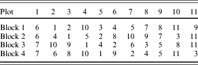
The following experiment serves as an illustration for the typical structure of such a rating experiment. Ten fungicide treatments were tested for their ability to protect potatoes against the attack by potato late blight (Phytophthora infestans). The experiment was performed as a randomized block design (Table 1), each block consisting of 11 plots arranged in a row in the experimental field. The 10 active treatments and a control, consisting of no treatment, were randomly applied to the plots. There were four replicates consisting of four neighbouring rows in the experimental field. The observations were taken after a week of moist weather conditions following a dry period. The observations were taken on the same day by four judges, called A, B, C and D. Judges A and B were experienced in the scoring procedure whereas judges C and D had never performed such a rating and they received a short introduction. The evaluations of the four judges were compared.
Randomized block design for the analysis of the effect of fungicides. The blocks were parallel rows in an experimental field. The numbers identify the fungicide treatments, the number one refers to untreated plots
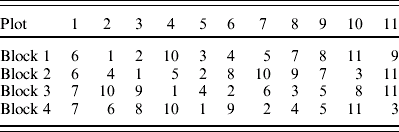
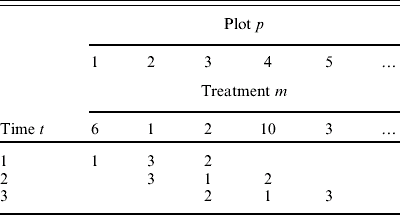
For comparison purposes, each judge first evaluated for each plot the proportion of the leaf area (L) destroyed by potato late blight. This was calculated by combining the proportion of leaves fallen to the ground and the proportion of unaffected leaves still on the plants. The proportions were obtained by visual inspection and were not based on counts of leaves. This proportion, which was later analysed by the traditional method, is referred to herein as the score rating. This rating was performed in the morning. In the afternoon the judges ranked the plots by giving a rank-order to all triples of neighbouring plots within all four blocks, e.g. ranking in block 1 the plots 1, 2, 3, then the plots 2, 3, 4, etc. Therefore, a judge evaluated N m=11 different treatments by ranking N r=3 consecutive plots at a time. Successive evaluations had an overlap of N o=2 plots. Table 2 shows the first three comparisons in the first block made by judge A.
The first three rank vectors by judge A. The corresponding rank-order vector at time 2 was O2=(3, 4, 2)
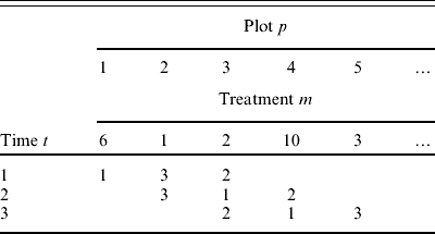
The variable ‘time’ gives the observation number for the rank vector. The ranking was such that the plot with the highest criterion value – here the proportion of preserved leaf area – was ranked highest, i.e. achieved the lowest rank number. The recorded observation was the rank-order of the plots. For example, at the time t=2, plot 3 was ranked highest, followed by plots 4 and 2; hence the recorded order was (3, 4, 2).
Thurstonian model of ranking
First, a Thurstonian latent variable model is introduced for the analysis of the rank-based observations. Later, a model for the analysis of the score observations is given.
It is assumed that, in each comparison, a judge compares latent random utilities for each plot and ranks these according to the utilities. The utility Y tp for a specific plot p at observation time t is given by

where μm denotes the mean utility for each treatment and m(p) is the mapping of the plots to the treatments. εtp∼N(0, σS2) are independently distributed perceptions errors and δp∼N(0, σP2) are plot-to-plot errors. Let Yt=(Y tp) be the vector of utilities at time t.
Let {p 1,…, p Nr} denote the set of plots observed at time t and let the utilities be ordered as  . Then the observed rank-order vector is Ot=O(Yt)=(p 1, p 2,…,p Nr) such that the highest ranked plot is given first. This model for rankings is known as the Thurstonian model (Thurstone Reference Thurstone1927; Böckenholt Reference Böckenholt, Fligner and Verducci1993).
The mean utilities μm are only defined up to a translation and only the differences μm−μm′ are of interest. Additionally, the scale may be arbitrarily fixed which is done by imposing the restriction σS2+σP2=1.
The following notation is used in the sequel: O=(Ot), Y=(Yt), μ=(μm), ε=(εtp) and U=(U p) where U p is defined as U p=μm(p)+δp.
The distribution of the rank-order vectors is specified as a hierarchical model.


, independent for all t, p

The model will be applied to the experimental data without accounting for the block structure because the comparative ranking within each block removes possible block effects. The model may be extended into several directions. Instead of comparing only unstructured treatments the model allows also for a factorial structure or linear model in the mean utilities μm. The aspect that spatially closer observations may be perceived as being more similar could be represented by an autocorrelation structure imposed on the perceptions errors εtp. This additional structure could easily be incorporated in the MCMC sampling process. Only the analysis for repeated measures taken by one judge was considered. For the analysis of several judges j one could add a random component εjm that would cover judge specific orderings of the crops.
Estimation in the Thurstonian model
The estimation of the parameters was by a Bayesian analysis. Additional to the specifications in Eqns (2)–(4) we provide a prior distribution f(η) for η=(μ, σP2). By Bayes theorem one obtains together with the likelihood f(o|η) the posterior distribution f post(η|o)=f(o|η)f(η)/∫f(o|η)f(η)dη. The estimation is then based on the posterior distribution. The prior distributions are specified as:

The equation on the right above specifies a non-informative prior for the variance σP2 that does not favour a specific value for σP2. The parameter σμ2 is a meta-parameter that is not estimated from the data but controls the prior distribution of μ. The variance σμ2 should be chosen large enough, such that the prior information about the scaling of the μm is non-informative in relation to the scale information expressed by the choice of σS2+σP2=1. In the simulation study the influence of the choices σμ2=50, 100, 200 were compared and in the analysis of the experiment σμ2=100 was used. The Eqns (5) and (2)–(4) express a Bayesian hierarchical model (Gelman et al. Reference Gelman, Carlin, Stern and Rubin2004, chapter 5). The likelihood is given as:

where f (u p|η) is the normal density given in Eqn (2) and  t(u|θ) is the evaluation of a N r−1 variate normal distribution function
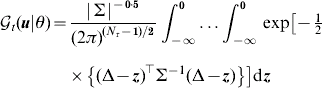
where Δk=u o(t, k)−u o(t, k−1) and Σ=σi, j is a (N r−1)×(N r−1) covariance matrix, such that σ i, i=2σS2, σi, i+1=σi+1, i=−σS2 and the other entries are zero. In the notation, the dependence of the likelihood on σμ2 was suppressed.
From the posterior distribution f post(η|o) the mean utility differences μm−μk were estimated as the posterior means  . The variability of the estimation of a difference μm−μk can be described by a posterior credibility interval for these differences. An alternative variability measure is the posterior probability (denoted by θmk) that μm is larger than μk. This probability is considered as a precision measure and used in the simulation study for efficiency comparisons under different design structures. The numerical analysis of the Thurstonian model was made by MCMC sampling (Gilks et al. Reference Gilks, Richardson and Spiegelhalter1996). With MCMC it is not necessary to calculate the posterior density by numerical integration. One generates samples from the posterior distribution of the parameters η exploiting the hierarchical structure of the model. The posterior means are calculated as the average of sampled parameters and 95% credible intervals are based on the sample 2·5 and 97·5% quantiles. This sampling was implemented with the software OpenBUGS (Thomas et al. Reference Thomas, O'Hara, Ligges and Sturtz2006). This software provides a general framework for the Bayesian analysis of a hierarchical model via MCMC sampling.
For each analysis, seven chains were generated from different starting values for the parameters. After each run, the convergence was checked by the Gelman–Rubin–Brooks statistic (Gelman & Rubin Reference Gelman and Rubin1992; Brooks & Gelman Reference Brooks and Gelman1998) and convergence was considered sufficient if the statistic was smaller than 1·1 (see Gelman et al. Reference Gelman, Carlin, Stern and Rubin2004, p. 297) for all the differences between μm−μ1 in the simulation study (μm−μ2 in the analysis of the experiment) and the chain for σP2. In the simulation study 10 000 samples were taken for each of seven chains (since the MCMC sample takes some time to converge to the posterior distribution, an initial 10 000 samples – termed burn-in samples – were discarded.
For the analysis of the experiment the samples had a length of 1 000 000 and the burn-in phase of 100 000. Only every 100th sample was kept for further analysis.
The general statistical programming environment R (R Development Core Team 2006) was used for the data analysis, in particular the package R2WinBUGS (Sturtz et al. Reference Sturtz, Ligges and Gelman2005) for running OpenBUGS from R and the package coda (Plummer et al. Reference Plummer, Best, Cowles and Vines2004) to calculate the Gelman–Rubin–Brooks convergence statistic.
An R-package to analyse the data of the experiment for judge A can be found online at http://gbi.agrsci.dk/~uhh/thurstrank.
Model for the relative scores
The score ratings were analysed by a regression model for the scores. First, the proportion of non-attacked leaf area 1−L was transformed with the logit function logit (x)=log (x/(1−x)) to obtain more symmetrically distributed responses. The following regression model was fitted

with the block effects αb, b=1,…, 4, treatment effects βm, 1,…, 11 and independently normally distributed errors e bm with a common variance.
Simulation study
The simulation study was performed for N m=7 treatments with the mean utilities μ=(0, 0·1, 0·3, 0·6, 1·0, 1·5 and 2·1). A design for the observations consisted of 52 consecutive plots, three neighbouring plots, N r=3, were to be ranked and two consecutive rankings had an overlap of two plots, N o=2. Hence there were 50 rank observations. The design was balanced such that all paired occurrences of two treatments were approximately equally represented over the set of ranking comparisons. The construction principle for the design was sequential. Assume, for example, that the ranking proceeds by advancing the ranking window by one plot and that a number of treatments are already placed on the first plots. For these treatments, the distribution of pairs of treatments in direct comparisons is determined. The treatment to be placed on the next plot is then chosen among those that maximally increase the entropy of this distribution.
For each plot a utility was generated according to model (1) with the variance σP2=0·4. The analysis was performed on 1000 generated designs with correspondingly generated random utilities.
The simulation study analyses the accuracy of the estimation of the parameters. The bias in estimating the difference for treatments of neighbouring size μm−μm−1 by the posterior mean  was estimated as the average across the simulations
 where
 is the posterior mean from the jth simulation. As an overall measure of accuracy, the root mean squared errors (RMSE) R m, m−1 of the are presented, estimated as
 , where V m, m−1 is the empirical variance of . For σP2 the average
 of the posterior means
 across the simulations is given and the estimate of the RMSE
 .
Additionally, the precision of estimating the difference between two neighbouring treatments was evaluated by looking at the average  across the simulations of the posterior probabilities θm, m−1 that μm>μm−1. These probabilities were compared to those from an analysis where the utilities Y tp were considered to be observed and analysed with a Bayesian hierarchical model described by the Eqns (2), (3) and (5).
The evaluation of the estimates was considered also for the following variations of the basic design:
• The effect of decreasing the overlap between two consecutive rankings from an overlap of two to an overlap of one and no overlap. These designs were derived from the basic designs by removing intermediate ranking comparisons. In the analysis of the design with no overlap the variance σP2 was removed from the model in Eqn (1) and σS2 was assumed to be 1.
• The effect of an unbalanced design. The generation of the designs was modified such that firstly the comparison of the treatments 1 and 2 did not occur and secondly the pairs (1,2), (1,3) and (1,4) did not occur.
• The effect of increasing the number of observations. A total of 150 designs were generated with an overlap of 2 and 1000 plots.
RESULTS
Simulation study
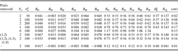
Table 3 summarizes the results for the simulation study for the analysis of the parameter estimates. In the first three rows the results are given for a design with an overlap of N o=2 for three different choices of the prior variance of μ. With one exception (for B 32 and σμ2=50) all the differences were positive. The bias was smaller than 0·02 for B 32 and B 43 but larger than 0·04 for the comparison between 1 and 2 and for the larger neighbouring treatment differences between 6 and 5 and between 7 and 6. The choice of the posterior variance σμ2 had no effect on the estimation as the B m, m−1 were similar across rows 1–3 in each column. Reducing the overlap (rows 4 and 5) to only 1 or no overlap increased the bias for all treatment comparisons and this increase was, with the exception of B 3,2, most pronounced for the no overlap case. Inducing imbalance to the design by removing some direct paired comparisons (rows 6 and 7) showed, in relation to row 2 only, a substantial increase in bias by 0·28 and 0·34 for the treatment comparison 7 to 6.
Results from the simulation study. The mean utilities from which the data were generated were μi=0, 0·1, 0·3, 0·6, 1·0, 1·5, 2·1 and the variance σP2=0·4. ‘Pairs removed’ denotes those paired comparisons that did not appear in any ranking comparison. No is the number of overlap between two consecutive rankings. Bm, m−1 is the estimated bias between the posterior mean to the model parameter  . Rm, m−1 is the estimated root mean squared error of .
 is the average across the simulations of the posterior means
 of the variance σP2 and
 denotes the root mean squared error. ‘conv’ denotes the proportion of simulations which did not converge. The simulations for the first seven rows were based on 52 plots and that for the last row on 1000 plots

The RMSEs R m,m−1 were very similar for the different prior variances σμ2 (rows 1–3) and differed by at most 0·02 in each column. Reducing the overlap from 2 to 1 increased the RMSEs for all comparisons by at least 0·19. The RMSEs were further increased when any overlap was removed.
Removing the direct comparisons between treatments 1 and 2 increased the RMSEs by 0·13 for the comparisons 2 to 1 (row 2 to row 6). The removal increased the RMSEs by 0·02 for the comparison 3 to 2 but decreased them for the other comparisons. Removing the direct comparisons between 1 and 2 and, in addition, those between treatments 1 and 3 and 1 and 4 increased the RMSEs further by 0·06 for the comparison 2 to 1 but decreased those for the comparisons 6 to 5 and 7 to 6.
In all cases the variance σP2 was estimated close to 0·4. The estimated and model generating parameters were almost identical for the simulations with 1000 observations and an overlap of two (last row of Table 3). Convergence problems of the MCMC sampling became more frequent with increasing variance for μ, by reducing the overlap or by increasing the imbalance of the design.
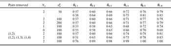
Table 4 shows the efficiency comparisons via the average of the posterior probabilities θm, m−1 between the different design structures. In rows 1, 3 and 4 the results are given for the overlap of 2 for the three different priors for μ. The values for the  within a column were almost identical and differed by at most 0·01. The precision increased with the treatment difference. Reducing the overlap by one decreased (comparing row 3 to 5) the precision by 0·02 for the lowest treatment difference and by 0·05 for the largest. The precisions dropped further by 0·05 for the largest treatment difference if the design contained no overlap. Dropping the direct comparison of the treatment 1 to 2 yielded similar precisions for the first three treatment comparisons compared to the balanced design. But for the three largest treatment differences the precisions were larger for the unbalanced design. Dropping all paired comparisons of treatment 1 to either treatment 2, 3 or 4 also yielded an increased precision for the three larger treatment comparisons but the precision for the lowest treatment difference dropped to 0·51. Using a design with 1000 plots yielded a precision of more than 0·99 for the three largest treatment differences and for the lowest treatment difference the precision was about 0·19 larger than in the case of 52 plots.
The means of the posterior probabilities θm,m−1 that μm is larger than μm−1. In the second row these probabilities are given for the parameter setting of row one but the rank-orders of the utilities were instead directly observed

Row 2 of Table 4 contains the results of an analysis directly on the utilities Y pm by which the rank observations for the simulations used for the row 1 were generated. There was a difference of 0·01 in the precision for the smallest treatment difference but the difference increased to 0·06 for the largest treatments 6 and 7.
Experiment
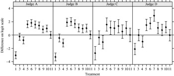
In Fig. 1, the estimated  and corresponding 95% confidence intervals are given for the score ratings by four judges A, B, C and D. Treatment 2 was chosen as the reference. There was almost complete agreement between the two experienced judges, A and B. The inexperienced judges, C and D, were less concordant with judges A and B. The confidence intervals for the treatment differences were larger for judges C and D than for the two experienced judges. All four judges evaluated the treatments 1, 3 and 4 as less effective than treatment 2, and the confidence intervals for treatments 1 and 4 did not include zero. All judges considered treatment 11 to be indistinguishable from treatment 2. The confidence intervals for the treatments 5 to 8 and 10 did not include zero for all judges.
The estimated differences in the percentage score on the logit scale with 95% confidence intervals. The differences are to the treatment 2.

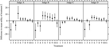
For the rank-based ratings, the differences of the posterior mean utilities to the mean utility of treatment 2 are given in Fig. 2 with 95% credibility intervals. All judges ranked treatment 1 lowest in all comparisons where this treatment occurred. This caused the difference of the mean utilities of the other treatments to this utility to be strongly dependent on the variance σμ2. Therefore, treatment 2 was chosen as the reference. As with the score ratings, all judges evaluated treatments 1 and 4 as worse than 2 with the upper credibility interval limit being lower than zero. Likewise, all judges evaluated treatments 5 to 7 to be larger than treatment 2, with the lower credibility interval limit being larger than zero. The widths of the credibility intervals were especially large for treatments 1 and 4 for judges A, B and D. For judge C, the width of the credibility interval for treatment 4 was comparable to the other intervals. In this context, it should be noted that judges A, B and D ranked treatment 4 lowest in rank order observations without treatment 1. Judge C had one instance where he ranked treatment 2 lower than treatment 4. For judge A, the credibility interval for treatment 5 was exceptionally large and this judge was the one who always ranked treatment 5 highest in the comparisons where it occurred. The other credibility intervals of judges A, C and D were comparable whereas those of judge B were larger.
The estimated differences in the mean utilities based on the ranked observations. The differences are to the treatment 2.

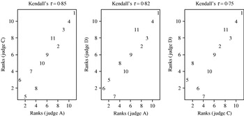
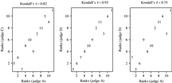
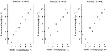
In Fig. 3, estimated treatment rank-orders based on the score ratings are compared between the judges A, C and D, while Fig. 4 provides the corresponding plots with the rank-orders based on the rank-based ratings. Judge B was not analysed here because he had the same estimated treatment rank-order as judge A in the score and the rank-based ratings. For the score ratings the treatment rank-order was taken as the ordering of the estimated . The treatment rank-order for the rank-based ratings was taken as the order of the mean utilities with the highest posterior probability.
Comparison of the treatment rank-orders between the judges A, C and D. The rank-orders are based on the rankings of the logits derived from the scores. The numbers are treatment indices.

Comparison of the treatment rank-orders between the judges A, C and D. The rank-orders are based on the rankings from the rank-based ratings.

The difference between the treatment rank-orders of judges A and D was larger for the score ratings than for the rank-based ratings. Judge C had about equal agreement with judge A in both methods. Judge A ranked treatment 6 highest in the score rating but treatment 5 in the rank-based rating.
A comparison between the treatment rank-orders obtained from the score ratings and the rank-based ratings are given for judges A, C and D in Fig. 5.
Comparison between the treatment rank-orders obtained from the rank-based ratings to those from the score ratings for the judges A, C and D.

The experienced judge A had only two reversals of the treatment rank order between the two observation methods, whereas judge C had changed the rank of treatment 8 by four positions and judge D had two reversals by two positions and one by three.
In Table 5, the estimates of the mean utilities are given for different choices of the variance σμ2 for μ. For a variance very small in relation to 1, the sum of the perception and the plot variance, the mean utilities (first row) were all very close to zero and small in relation to their posterior standard deviation. For the three treatments 1, 4 and 5 the differences tended to increase within increasing σμ2. For the other treatments the difference of the mean utilities stabilized for increasing σμ2.
Posterior means  and standard deviations (Sm, 2) of the posterior distribution of μm−μ2 for the data of judge A for different variances σμ2.
 is the posterior mean of


Finally, it should be noted that judges B and D, by moving on by one plot, always consistently ranked the two treatments from the overlapping plots in the same order. Judges A and C deviated in three and one cases, respectively, from this consistency.
DISCUSSION
The proposed model allowed the analysis of correlated rank observations. The application of the method is not restricted to crop experimentation but may be applied to any measurements where human evaluations are the basic measurement mode. The method may be a competitor to paired comparisons procedures without overlap, especially in the case of one judge with a limited number of replicates. The usage of overlapping observations showed a gain in precision of the estimated treatment differences. The most obvious explanation for the large loss in precision for the non-overlapping case observed in the simulation study is the reduction of the number of rank observations from 50 to 17. Thus the usage of repeated observations better exploited the experimental material.
In the simulation study, there was some indication that the differences in utilities tended to be overestimated for larger treatment differences. The posterior probability for a treatment difference to be larger than 0 was smaller for the rank-based ratings than from an analysis of the utilities themselves. This seems to be plausible as the loss of information incurred by observing only the rank information should yield a less stringent differentiation between the treatments.
The results of the simulation study showed that it is desirable for the numbers of direct comparisons within ranking observations between any two treatments to be approximately equal. In the present study, this was achieved by a sequential construction of the designs for the simulation study. Classical construction methods for optimal design do not seem to be applicable because they do not work on ranking observations, nor do they consider the moving window observation modus. The block randomization used for the present experiment obviously could not achieve a balance with respect to the number of direct treatment comparisons. Additionally, the number of blocks was too small in relation to the number of treatments to obtain such a balance.
The proposed method showed comparable results to a traditional ANOVA analysis in the experiment. It can be expected that the new method is faster to use than the traditional method and that it depends less on the experience or training of a judge to acquire the skill of accurate visual inspection. Both inexperienced judges felt that they understood the rank rating more easily than the more elaborate relative scoring; however in the present experiment this did not lead to a significantly improved rating.
If a treatment is always ranked highest in the rank-based rating, then any very large mean utility larger than the mean utilities for the other treatments will explain the data almost equally well. Only the variance imposed on μ will restrain the mean utility of that treatment from being estimated as infinity. Therefore, the estimated treatment differences involving that treatment will strongly depend on σμ2. The corresponding credibility intervals should therefore be considered with caution. A similar problem occurs in logistic regression in the case of separability of the binary observations with respect to one regressor. One solution proposed by Firth (Reference Firth, Fahrmeir, Francis, Gilchrist and Tutz1992) for these models is a penalized maximum likelihood approach, which resembles a Bayesian analysis with a Jeffrey's prior on the parameters. If there are only few treatments that are not linked to the others it might be acceptable to remove them from the analysis by the Thurstonian model.
A Bayesian approach was adopted in the present study mainly for computational reasons. The evaluation of the likelihood across the latent variables in the Thurstonian model poses a difficult numerical problem (Yao & Böckenholt Reference Yao and Böckenholt1999). In contrast to linear mixed models, the integral of the likelihood over the latent variables is not available in closed form and must be computed by numerical integration. The MCMC approach is a well-established method to obtain samples from the posterior distribution and to evaluate estimates as posterior means by averaging across the samples (Gilks et al. Reference Gilks, Richardson and Spiegelhalter1996). The availability of the OpenBUGS program facilitates the computational implementation, especially for the class of Bayesian hierarchical models. The Bayesian approach is sometimes considered to have a drawback compared to a likelihood approach because one has to specify a prior distribution which may unduly influence the inference. In the present paper, this problem was addressed by choosing a non-informative prior for the perception variance and showing that the estimation was not influenced over a wide range of the prior variance for the mean utilities. The strong dependence of some estimates on this prior variance occurred in a situation of no observed connection between two treatments. This is a situation where the corresponding maximum likelihood estimate does not exist.
The computations for the Bayesian approach for analysing the Thurstonian model were feasible with the MCMC method using OpenBUGS. The simulation study showed that in order to avoid convergence problems one should aim at using approximately balanced designs.
The authors thank Bent Nielsen, Research Centre Flakkebjerg, Faculty of Agricultural Sciences, University of Aarhus, who made it possible to perform the presented experiment within a larger experimental frame.