1 Introduction
Plasma solitons have been widely observed in the Earth’s magnetosphere. On ion-acoustic (IA) scales, these structures were observed in the auroral acceleration region (Temerin et al. Reference Temerin, Cerny, Lotko and Mozer1982; Koskinen, Lundin & Holback Reference Koskinen, Lundin and Holback1990; Mälkki et al. Reference Mälkki, Eriksson, Dovner, Boström, Holback, Holmgren and Koskinen1993). The negative polarity of these solitons is opposite or ‘anomalous’ (Baluku, Hellberg & Verheest Reference Baluku, Hellberg and Verheest2010b ) in comparison to the simplest fluid models of IA solitons (Washimi & Taniuti Reference Washimi and Taniuti1966). The study of this so-called ‘anomalous’ soliton polarity has led to a large body of theoretical studies.
From these studies, we can conclude that the negative polarity is the result of complex plasma compositions. However, the plasma species responsible for the opposite polarity is not well understood. In particular, it is not known whether this is the result of non-thermal electron distributions or multiple ion species.
The presence of non-thermal electrons can give rise to ‘anomalous’ negative polarity solitons. This can happen when electron distributions can be described by two-temperature electrons (Buti Reference Buti1980; Baluku & Hellberg Reference Baluku and Hellberg2012) or Cairns-distributed electrons (Cairns et al. Reference Cairns, Mamun, Bingham, Böstrom, Dendy, Nairn and Shukla1995). Alternatively, the presence of a second ion species may give rise to a so-called ‘slow IA mode’. Under suitable conditions, this slow mode can give rise to negative polarity IA solitons (Verheest et al. Reference Verheest, Hellberg, Saini and Kourakis2011; Lakhina, Singh & Kakad Reference Lakhina, Singh and Kakad2014; Olivier, Maharaj & Bharuthram Reference Olivier, Maharaj and Bharuthram2015). While both these types of models produce the desired polarity, it is difficult to determine which one is responsible for the observation of negative polarity solitons. In order to determine the correct mechanism directly, one has to have intimate knowledge of the plasma composition. Such detailed knowledge is usually not available from satellite observations.
One possible way around this would be the identification of coexistence. For plasmas associated with a second adiabatic species, there is usually no coexistence (Verheest et al. Reference Verheest, Hellberg, Saini and Kourakis2011; Lakhina et al. Reference Lakhina, Singh and Kakad2014). On the other hand, coexistence is associated with the presence of non-thermal electron distributions (Buti Reference Buti1980; Cairns et al. Reference Cairns, Mamun, Bingham, Böstrom, Dendy, Nairn and Shukla1995; Baluku & Hellberg Reference Baluku and Hellberg2012). Here, coexistence refers to the case where two soliton solutions exist for both positive and negative polarity. It is important to note that coexistence does not refer to a type of superposition of more than one bipolar electric field pulse. Instead, coexistence refers to the existence of separate solutions of a boundary value problem associated with a particular plasma composition and a fixed Mach number. The presence of coexistence would strongly suggest that non-thermal electron distributions are responsible for the negative polarity IA solitons.
Plasma compositions that support coexistence are characterized by two families of solitons with opposite polarities. The two families can be classified as either KdV-like or non-KdV-like. Here KdV-like (non-KdV-like) families have the property that the amplitude of the solitons vanishes (does not vanish) in the acoustic speed limit. The vanishing soliton amplitude property is consistent with the Korteweg–de Vries (KdV) equation that is derived from reductive perturbation analysis. Unless the plasma composition is critical (Olivier, Verheest & Maharaj Reference Olivier, Verheest and Maharaj2016), coexistence consists of a KdV-like and a non-KdV-like family of soliton solutions.
Baluku et al. (Reference Baluku, Hellberg, Kourakis and Saini2010a ) recently showed that coexistence is associated with acoustic speed solitons. They showed this for a plasma consisting of cold dust, adiabatic ions and kappa-distributed electrons. Since then, acoustic speed solitons were reported for a wide range of plasma compositions that exhibit coexistence (Baluku et al. Reference Baluku, Hellberg and Verheest2010b ; Baluku & Hellberg Reference Baluku and Hellberg2011; Verheest Reference Verheest2011). In addition, acoustic speed double layers were reported (Verheest, Hellberg & Baluku Reference Verheest, Hellberg and Baluku2012; Olivier et al. Reference Olivier, Maharaj and Bharuthram2015), while Verheest & Hellberg (Reference Verheest and Hellberg2015) reported acoustic speed supersolitons. These acoustic speed nonlinear structures form in non-KdV-like families of solitons.
To our knowledge, acoustic speed solitons have not been reported by satellite observations or by experimental studies. To do so, one would need (i) an exact measurement of the acoustic speed and (ii) an exact measurement of the soliton velocity. This is not very practical, as both these velocities are difficult to measure directly, and are usually estimated through some approximation. It would therefore be useful to establish a different characteristic of acoustic speed solitons that is easier to measure.
We recently reported a promising result in the form of an analytical solution for small-amplitude acoustic speed solitons near critical plasma compositions (Olivier et al. Reference Olivier, Verheest and Maharaj2016). The resulting soliton consists of a Lorentzian pulse. The tails of Lorentzian pulses decay at an algebraic rate, which is much slower than the exponential decay rate observed in regular solitons. Therefore, in the small-amplitude regime, acoustic speed solitons can be identified by their fat tails.
In this paper we use Sagdeev theory to extend this result to acoustic speed solitons of arbitrary amplitude. We therefore propose that the tails can be used to identify solitons, double layers and supersolitons that propagate at the acoustic speed. This, in turn, can be used to identify coexistence. As mentioned above, this identification would suggest that non-thermal electrons are responsible for the formation of negative polarity IA solitons in space plasmas.
It is important to point out some issues that have to be taken into account when applying the results of our asymptotic study. Firstly, Sagdeev potential analysis applies to fluid models where kinetic effects are neglected. Simulation studies have shown that kinetic effects may significantly alter soliton solutions (Kakad, Kakad & Omura Reference Kakad, Kakad and Omura2014; Jenab & Spanier Reference Jenab and Spanier2017). Secondly, Sagdeev pseudopotential analysis considers an idealized situation where only a single soliton is excited. Consequently, important topics such as the interaction properties and generation mechanisms of solitons fall outside the scope of Sagdeev pseudopotential analysis. The former is especially important for the study of space plasmas where solitons are often observed in clusters (see for example Bounds et al. Reference Bounds, Pfaff, Knowlton, Mozer, Temerin and Kletzing1999). The generation and interaction properties of acoustic speed solitons with (a) other solitons, (b) linear waves and (c) background noise may be studied by considering systems where the initial plasma state can be controlled. Such systems can be realized in simulation studies (Kakad, Omura & Kakad Reference Kakad, Omura and Kakad2013; Kakad, Lotekar & Kakad Reference Kakad, Lotekar and Kakad2016; Lotekar, Kakad & Kakad Reference Lotekar, Kakad and Kakad2016) and in laboratory experiments (see for example Nakamura & Tsukabayashi Reference Nakamura and Tsukabayashi1984). These considerations are, however, beyond the scope of this paper.
The paper is structured as follows: in § 2 we show that acoustic speed solitons decay at an algebraic rate, irrespective of the size of their amplitudes. In § 3 we consider acoustic speed double layers. We show that only one of the double layer tails decay algebraically as a result of the acoustic speed propagation. We also show that the other tail decays at the much slower algebraic rate when the Sagdeev potential has a triple root. In § 4 we illustrate the results by means of a case study for a fluid model consisting of two cold ion species and Cairns-distributed electrons, based on the study of Verheest & Hellberg (Reference Verheest and Hellberg2015). In § 5, our conclusions are presented.
2 Asymptotic behaviour of solitons and supersolitons
We use the ideas of our earlier paper (Olivier et al.
Reference Olivier, Verheest and Maharaj2016) by considering a generalized fluid plasma model with a Sagdeev potential
 $V(\unicode[STIX]{x1D719},M)$
that satisfies the energy-like integral
 $$\begin{eqnarray}\frac{1}{2}\left(\frac{\text{d}\unicode[STIX]{x1D719}}{\text{d}\unicode[STIX]{x1D709}}\right)^{2}+V(\unicode[STIX]{x1D719},M)=0.\end{eqnarray}$$
The difference here is that we consider only the tail of the soliton, so that we are restricted to small disturbances in the electrostatic potential. As a result, we only need to consider the shape of the Sagdeev potential
 $V(\unicode[STIX]{x1D719},M)$
in the vicinity of the equilibrium electrostatic potential
 $\unicode[STIX]{x1D719}=0$
.
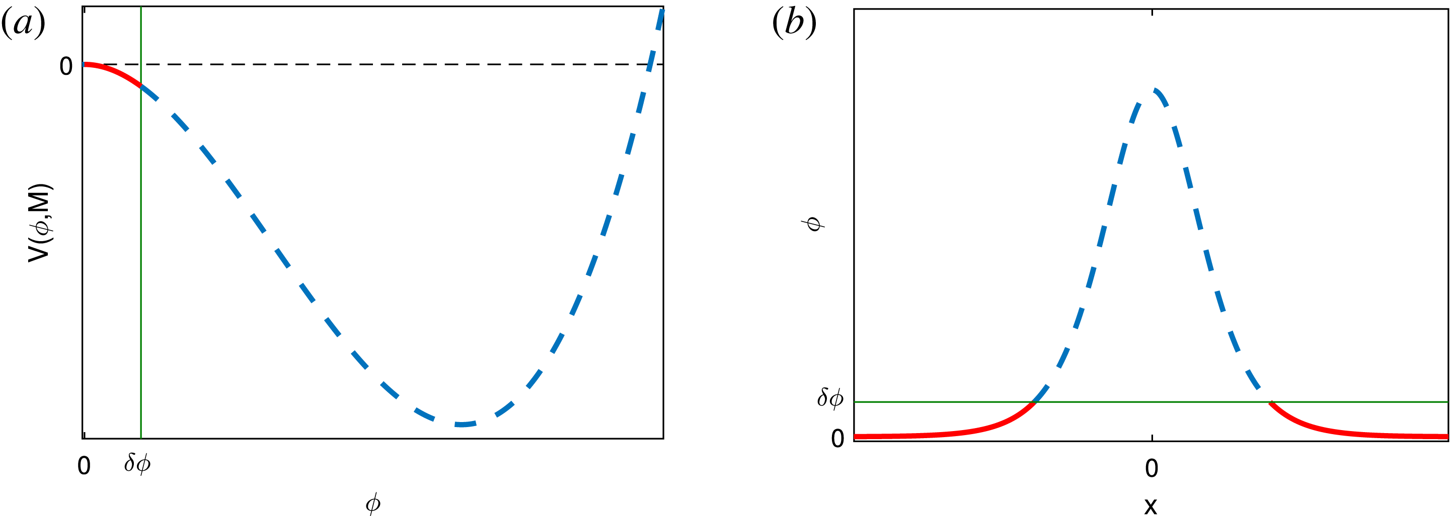
Graphical representation of the asymptotic expansion. In (a), a typical Sagdeev potential is shown, while in (b), the corresponding soliton solution is shown.

This approach can be explained by considering the graphical illustration in figure 1. A typical Sagdeev potential is shown in figure 1(a). The thin vertical line (green online) corresponds to a small but finite electrostatic potential
 $\unicode[STIX]{x1D6FF}\unicode[STIX]{x1D719}$
. The soliton solution for
 $0<\unicode[STIX]{x1D719}<\unicode[STIX]{x1D6FF}\unicode[STIX]{x1D719}$
is governed by the Sagdeev potential to the left of this vertical line, shown as the thick solid line (red online), while the core of the soliton is governed by the part of the Sagdeev potential shown as a dashed line (blue online).
The soliton associated with this Sagdeev potential is shown in figure 1(b). The thin horizontal line (green online) again indicates the small electrostatic potential
 $\unicode[STIX]{x1D6FF}\unicode[STIX]{x1D719}$
. The tails of the soliton form below this line, shown by the thick solid lines (red online). On the other hand, the core of the soliton is formed above the thin horizontal line, and is indicated by the dashed line (blue online).
The idea behind our approach is to use a Taylor series expansion to obtain a simple expression for the Sagdeev potential near the equilibrium, i.e. the part illustrated by the thick solid line to the left of
 $\unicode[STIX]{x1D6FF}\unicode[STIX]{x1D719}$
in figure 1(a). By substituting this expression into the energy integral (2.1) and integrating, we can then obtain an analytical expression for the tails of the soliton, as illustrated by the solid lines below
 $\unicode[STIX]{x1D6FF}\unicode[STIX]{x1D719}$
in figure 1(b). In the limit
 $\unicode[STIX]{x1D6FF}\unicode[STIX]{x1D719}\rightarrow 0$
, this approximation converges to an exact expression for the tails of the soliton.
Therefore, the first step is to apply a Taylor series expansion of the function
 $V(\unicode[STIX]{x1D719},M)$
about the equilibrium density
 $\unicode[STIX]{x1D719}=0$
. By convention, the Sagdeev potential is constructed in such a way that
 $V(0,M)=0$
. In addition, the charge neutrality at equilibrium ensures that
 $\unicode[STIX]{x2202}V/\unicode[STIX]{x2202}\unicode[STIX]{x1D719}(0,M)=0$
. From this, it follows that the lowest-order terms of a Taylor series expanded about the equilibrium potential
 $\unicode[STIX]{x1D719}=0$
are given by:
 $$\begin{eqnarray}V(\unicode[STIX]{x1D719},M)=B(M)\unicode[STIX]{x1D719}^{2}+C(M)\unicode[STIX]{x1D719}^{3}+O(\unicode[STIX]{x1D719}^{4}).\end{eqnarray}$$
The constants are defined as
 $$\begin{eqnarray}B(M)=\frac{1}{2}\frac{\unicode[STIX]{x2202}^{2}V}{\unicode[STIX]{x2202}\unicode[STIX]{x1D719}^{2}}(0,M),\quad C(M)=\frac{1}{6}\frac{\unicode[STIX]{x2202}^{3}V}{\unicode[STIX]{x2202}\unicode[STIX]{x1D719}^{3}}(0,M).\end{eqnarray}$$
For ease of presentation, we drop the
 $M$
dependence of the coefficients
 $B$
and
 $C$
throughout the rest of the paper.
There are two conditions for the existence of solitons that propagate faster than the acoustic speed. Firstly, one must have
 $B<0$
. Secondly, the Sagdeev potential
 $V(\unicode[STIX]{x1D719},M)$
must have a non-zero root
 $\unicode[STIX]{x1D719}_{r}$
where
 $V(\unicode[STIX]{x1D719}_{r},M)=0$
. If the Sagdeev potential has a positive and a negative root, then the coexistence of a positive polarity soliton and a negative polarity soliton arises.
The acoustic speed
 $M_{a}$
forms the lower limit of soliton velocities. Here, the acoustic speed is the critical velocity that satisfies the property
 $B=0$
, for
 $B$
defined in (2.3a
). Here we consider non-critical plasma compositions that satisfy
 $C\neq 0$
. In such a case, an acoustic speed soliton exists provided that the Sagdeev potential has a root
 $\unicode[STIX]{x1D719}_{r}$
with the opposite sign of
 $C$
, i.e.
 $C\unicode[STIX]{x1D719}_{r}<0$
.
The boundary condition
 $\unicode[STIX]{x1D719}\rightarrow 0$
as
 $\unicode[STIX]{x1D709}\rightarrow \pm \infty$
ensures that the lowest-order term in the Taylor series (2.2) will dominate the Sagdeev potential whenever
 $|\unicode[STIX]{x1D709}|$
is sufficiently large. One therefore gets
 $$\begin{eqnarray}V(\unicode[STIX]{x1D719},M)\approx B\unicode[STIX]{x1D719}^{2}.\end{eqnarray}$$
On the other hand, at the acoustic speed
 $M_{a}$
the second-order contribution vanishes since
 $B=0$
. Therefore, the lowest-order contribution is given by
 $$\begin{eqnarray}V(\unicode[STIX]{x1D719},M_{a})\approx C\unicode[STIX]{x1D719}^{3}.\end{eqnarray}$$
For super-acoustic speed (regular) solitons, one has the property that
 $B<0$
. In the limit
 $|\unicode[STIX]{x1D709}|\rightarrow \infty$
, it follows that
 $|\unicode[STIX]{x1D719}|\rightarrow 0$
. Therefore, the lowest order term of the Taylor series expansion (2.2) will dominate the dynamics. In this regime, the Sagdeev potential can be approximated by (2.4). By substituting this expression into the energy-like integral (2.1), one obtains the equation
 $$\begin{eqnarray}\frac{1}{2}\left(\frac{\text{d}\unicode[STIX]{x1D719}}{\text{d}\unicode[STIX]{x1D709}}\right)^{2}+B\unicode[STIX]{x1D719}^{2}=0.\end{eqnarray}$$
This can be simplified to obtain the following differential equation:
 $$\begin{eqnarray}\frac{\text{d}\unicode[STIX]{x1D719}}{\text{d}\unicode[STIX]{x1D709}}=\pm \sqrt{-2B\unicode[STIX]{x1D719}^{2}}.\end{eqnarray}$$
This equation can be written as a separable equation:
 $$\begin{eqnarray}\frac{\text{d}\unicode[STIX]{x1D719}}{\unicode[STIX]{x1D719}}=\pm \sqrt{-2B}\,\text{d}\unicode[STIX]{x1D709}.\end{eqnarray}$$
Integration of (2.8) and simplification leads to the following limit in the
 $|\unicode[STIX]{x1D709}|\rightarrow \infty$
regime:
 $$\begin{eqnarray}\unicode[STIX]{x1D719}(\unicode[STIX]{x1D709})\rightarrow \unicode[STIX]{x1D6FC}\exp \left(\pm \sqrt{-2B}\unicode[STIX]{x1D709}\right).\end{eqnarray}$$
Here the upper (plus) sign and the lower (minus) sign correspond to the limits
 $\unicode[STIX]{x1D709}\rightarrow -\infty$
and
 $\unicode[STIX]{x1D709}\rightarrow +\infty$
, respectively. In addition, the sign of the constant of integration
 $\unicode[STIX]{x1D6FC}$
is the same as the sign of the root
 $\unicode[STIX]{x1D719}_{r}$
.
The result shows that the tail of any regular soliton that propagates faster than the acoustic speed decays at a rate proportional to
 $\unicode[STIX]{x1D719}\propto \exp (-\sqrt{-2B}|\unicode[STIX]{x1D709}|)$
in the limit
 $|\unicode[STIX]{x1D709}|\rightarrow \infty$
.
At the acoustic speed
 $M_{a}$
, the dominant term in the
 $|\unicode[STIX]{x1D709}|\rightarrow \infty$
limit is given by (2.5). If we substitute this expression into the energy-like integral (2.1), one obtains the following equation:
 $$\begin{eqnarray}\frac{1}{2}\left(\frac{\text{d}\unicode[STIX]{x1D719}}{\text{d}\unicode[STIX]{x1D709}}\right)^{2}=-C\unicode[STIX]{x1D719}^{3}.\end{eqnarray}$$
If we simplify this expression, one obtains
 $$\begin{eqnarray}\frac{\text{d}\unicode[STIX]{x1D719}}{\text{d}\unicode[STIX]{x1D709}}=\pm \sqrt{-2C\unicode[STIX]{x1D719}^{3}}.\end{eqnarray}$$
For the expression on the right-hand side to remain real, it follows that the sign of
 $\unicode[STIX]{x1D719}$
should be the opposite of
 $C$
. One can write (2.11) as a separable equation
 $$\begin{eqnarray}\left.\begin{array}{@{}c@{}}\unicode[STIX]{x2460}\qquad \unicode[STIX]{x2461}\qquad \unicode[STIX]{x2462}\\ \displaystyle \displaystyle \frac{\text{d}\unicode[STIX]{x1D719}}{(\pm \unicode[STIX]{x1D719})^{3/2}}=\pm \displaystyle \sqrt{\mp 2C}\,\text{d}\unicode[STIX]{x1D709}.\end{array}\right\}\end{eqnarray}$$
In (2.12), we use the labels
 $\unicode[STIX]{x2460}$
–
 $\unicode[STIX]{x2462}$
to point out the different
 $\pm /\mp$
signs. For
 $\unicode[STIX]{x1D719}>0$
and
 $C<0$
, the upper (plus) and upper (minus) signs must be used in terms
 $\unicode[STIX]{x2460}$
and
 $\unicode[STIX]{x2462}$
, respectively. Conversely, for
 $\unicode[STIX]{x1D719}<0$
and
 $C>0$
, the lower (minus) and lower (plus) signs must be used in terms
 $\unicode[STIX]{x2460}$
and
 $\unicode[STIX]{x2462}$
, respectively. The
 $\pm$
sign in term
 $\unicode[STIX]{x2461}$
has a different meaning. It corresponds to the direction of the fictitious particle in the energy integral analogy. Therefore, both signs must be retained, irrespective of the sign of
 $C$
.
Integration of (2.12) gives
 $$\begin{eqnarray}-\frac{2}{\sqrt{\pm \unicode[STIX]{x1D719}}}=\pm \sqrt{\mp 2C}\left(\unicode[STIX]{x1D709}-\unicode[STIX]{x1D709}_{0}\right),\end{eqnarray}$$
where
 $\unicode[STIX]{x1D709}_{0}$
is a constant of integration. From (2.13) it follows that
 $$\begin{eqnarray}\pm \unicode[STIX]{x1D719}=\mp \frac{2}{C(\unicode[STIX]{x1D709}-\unicode[STIX]{x1D709}_{0})^{2}}.\end{eqnarray}$$
Here, the upper (plus) sign on the left-hand side and the upper (minus) sign on the right-hand side correspond to
 $C<0$
. Conversely, the lower (minus) sign on the left-hand side and the lower (plus) sign on the right-hand side correspond to the case where
 $C>0$
. As a result, equation (2.14) reduces to
 $$\begin{eqnarray}\unicode[STIX]{x1D719}=-\frac{2}{C(\unicode[STIX]{x1D709}-\unicode[STIX]{x1D709}_{0})^{2}}.\end{eqnarray}$$
In the relevant
 $|\unicode[STIX]{x1D709}|\rightarrow \infty$
limit, one obtains that
 $$\begin{eqnarray}\unicode[STIX]{x1D719}\propto \frac{1}{\unicode[STIX]{x1D709}^{2}}.\end{eqnarray}$$
For any fixed value of
 $t$
, the decay rate of the acoustic speed soliton is only algebraic at a rate proportional to
 $x^{-2}$
. This is clearly much slower than the exponential decay rate of regular solitons (2.9).
3 Asymptotic behaviour of double layers
The difference between solitons and double layers is that the non-zero root of the corresponding Sagdeev potential forms a multiple root in the latter case. In most cases, this consists of a double root, i.e. a local maximum. The resulting double layer solutions form ramp-like structures in the electrostatic potential.
Before we discuss the difference between regular double layers and acoustic speed double layers, we need to discuss the boundary conditions. For solitons and supersolitons, one has that
 $\unicode[STIX]{x1D719}\rightarrow 0$
when
 $|\unicode[STIX]{x1D709}|\rightarrow \infty$
. For double layers, these boundary conditions are violated, as the limits of
 $\unicode[STIX]{x1D719}$
differ for the limits
 $\unicode[STIX]{x1D709}\rightarrow -\infty$
and
 $\unicode[STIX]{x1D709}\rightarrow +\infty$
.
In constructing the double layer solutions, there are two different views on how to deal with the boundary conditions. On the one hand, one may treat the solution as a shock wave. In this case, the right-hand side of the double layer is treated as an undisturbed ‘downstream’ region, so that
 $\unicode[STIX]{x1D719}\rightarrow 0$
when
 $\unicode[STIX]{x1D709}\rightarrow +\infty$
. If the root of the Sagdeev potential is given by
 $\unicode[STIX]{x1D719}_{DL}$
, it follows that the double layer solution satisfies the boundary condition
 $\unicode[STIX]{x1D719}\rightarrow \unicode[STIX]{x1D719}_{DL}$
when
 $\unicode[STIX]{x1D709}\rightarrow -\infty$
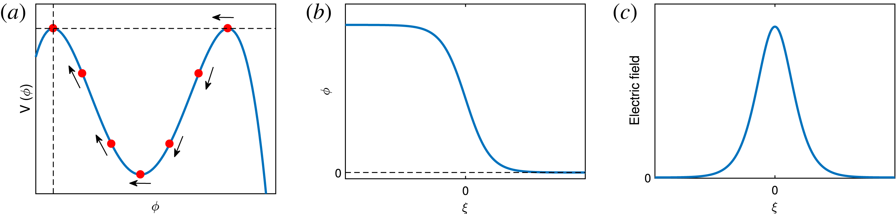
. This case is illustrated in figure 2.
Graphical illustration of a positive polarity double layer with boundary conditions
 $\unicode[STIX]{x1D719}\rightarrow 0$
when
 $\unicode[STIX]{x1D709}\rightarrow +\infty$
. In (a), the Sagdeev potential and motion of the fictitious particle is shown. In (b) and (c), the resulting electrostatic potential profile and the electric field profile are shown, respectively.

Graphical illustration of a positive polarity double layer with boundary conditions
 $\unicode[STIX]{x1D719}\rightarrow 0$
when
 $\unicode[STIX]{x1D709}\rightarrow -\infty$
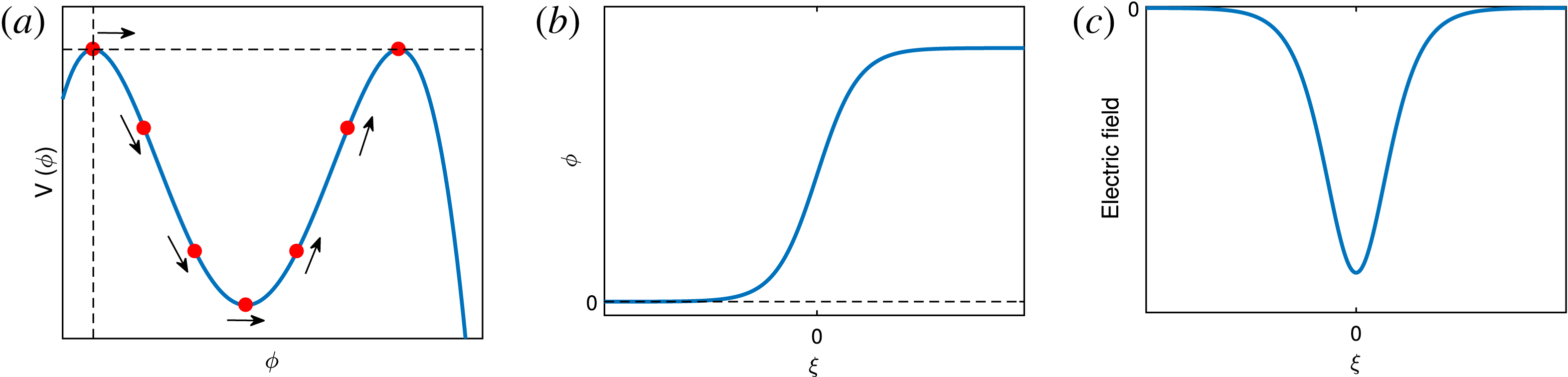
. In (a), the Sagdeev potential and motion of the fictitious particle is shown. In (b) and (c), the resulting electrostatic potential profile and the electric field profile are shown, respectively.

The alternative view is perhaps best described by considering the Sagdeev pseudopotential formalism. In the energy integral analogy, the solution corresponds to the motion of a fictitious particle in an undamped potential well
 $V(\unicode[STIX]{x1D719},M)$
. If the solution is treated as a small perturbation from the origin, it means that the particle starts off at the origin. However, due to the second potential hill, the particle never returns to the original position. Instead, it approaches
 $\unicode[STIX]{x1D719}\rightarrow \unicode[STIX]{x1D719}_{DL}$
as
 $\unicode[STIX]{x1D709}\rightarrow +\infty$
. Therefore, the corresponding boundary conditions are given as follows:
 $\unicode[STIX]{x1D719}\rightarrow 0$
when
 $\unicode[STIX]{x1D709}\rightarrow -\infty$
and
 $\unicode[STIX]{x1D719}\rightarrow \unicode[STIX]{x1D719}_{DL}$
when
 $\unicode[STIX]{x1D709}\rightarrow +\infty$
. This set of boundary conditions is illustrated in figure 3.
By comparing the two solutions, we see that the same Sagdeev potential produces electric field pulses with opposite polarities. Therefore, the solutions are very different for the different sets of boundary conditions. One may therefore ask: which of the two is correct? The answer is that either solution may be correct, depending on the underlying physical system. Importantly, the correct solution does not depend on the sign of the double layer root
 $\unicode[STIX]{x1D719}_{DL}$
. Rather, it depends on the boundary conditions of the underlying physical system. Throughout the paper we consider the former approach, namely that
 $\unicode[STIX]{x1D719}\rightarrow 0$
when
 $\unicode[STIX]{x1D709}\rightarrow +\infty$
. However, the results can easily be extended to the alternative set of boundary conditions.
We can now consider the tails of the double layer. It is important to note that the Sagdeev potential in the vicinity of the origin describes only one side of the tail, namely the side that approaches
 $\unicode[STIX]{x1D719}=0$
. For our chosen boundary conditions, this corresponds to the tail on the right-hand side of the double layer solution.
The results obtained in § 2 can easily be extended to double layers. For double layers propagating faster than the acoustic speed with velocity
 $M_{DL}>M_{a}$
, it follows directly from (2.9) that
 $$\begin{eqnarray}\unicode[STIX]{x1D719}(\unicode[STIX]{x1D709})\rightarrow \unicode[STIX]{x1D6FC}\text{e}^{-\sqrt{-2B}\unicode[STIX]{x1D709}}\end{eqnarray}$$
in the limit
 $\unicode[STIX]{x1D709}\rightarrow +\infty$
, where
 $\unicode[STIX]{x1D6FC}$
is an integration constant. On the other hand, for a double layer that propagates at the acoustic speed
 $M_{DL}=M_{a}$
, it follows directly from (2.15) that
 $$\begin{eqnarray}\unicode[STIX]{x1D719}(\unicode[STIX]{x1D709})\rightarrow -\frac{2}{C(\unicode[STIX]{x1D709}-\unicode[STIX]{x1D709}_{0})^{2}}\end{eqnarray}$$
in the limit when
 $\unicode[STIX]{x1D709}\rightarrow +\infty$
.
In order to resolve the tail on the left-hand side, we need to consider the Sagdeev potential in the limit
 $\unicode[STIX]{x1D709}\rightarrow -\infty$
. In this limit, the electrostatic potential approaches the multiple root
 $\unicode[STIX]{x1D719}\rightarrow \unicode[STIX]{x1D719}_{DL}$
.
To study the asymptotic behaviour of this tail, we may expand the Sagdeev potential about the double layer root
 $\unicode[STIX]{x1D719}=\unicode[STIX]{x1D719}_{DL}$
to get
 $$\begin{eqnarray}V\left(\unicode[STIX]{x1D719}\right)\approx V\left(\unicode[STIX]{x1D719}_{DL}\right)+\unicode[STIX]{x1D6FF}\unicode[STIX]{x1D719}\frac{\unicode[STIX]{x2202}V}{\unicode[STIX]{x2202}\unicode[STIX]{x1D719}}\left(\unicode[STIX]{x1D719}_{DL}\right)+\frac{1}{2}\unicode[STIX]{x1D6FF}\unicode[STIX]{x1D719}^{2}\frac{\unicode[STIX]{x2202}^{2}V}{\unicode[STIX]{x2202}\unicode[STIX]{x1D719}^{2}}\left(\unicode[STIX]{x1D719}_{DL}\right)+\frac{1}{6}\unicode[STIX]{x1D6FF}\unicode[STIX]{x1D719}^{3}\frac{\unicode[STIX]{x2202}^{3}V}{\unicode[STIX]{x2202}\unicode[STIX]{x1D719}^{3}}\left(\unicode[STIX]{x1D719}_{DL}\right)+\cdots \,,\end{eqnarray}$$
where
 $\unicode[STIX]{x1D719}=\unicode[STIX]{x1D719}_{DL}+\unicode[STIX]{x1D6FF}\unicode[STIX]{x1D719}$
. In this expansion (and throughout this section), the double layer velocity
 $M=M_{DL}$
is chosen.
Since
 $\unicode[STIX]{x1D719}_{DL}$
is a root of the Sagdeev potential, it follows that
 $V(\unicode[STIX]{x1D719}_{DL})=0$
. In addition, since we have a double layer, the multiplicity of the root is higher than one. It follows that the first derivative also vanishes. We can therefore simplify the Taylor series expansion (3.3) to the form
 $$\begin{eqnarray}V(\unicode[STIX]{x1D719}_{DL}+\unicode[STIX]{x1D6FF}\unicode[STIX]{x1D719})\approx B_{DL}\unicode[STIX]{x1D6FF}\unicode[STIX]{x1D719}^{2}+C_{DL}\unicode[STIX]{x1D6FF}\unicode[STIX]{x1D719}^{3}+O(\unicode[STIX]{x1D6FF}\unicode[STIX]{x1D719}^{4}).\end{eqnarray}$$
Here
 $$\begin{eqnarray}B_{DL}=\frac{1}{2}\frac{\unicode[STIX]{x2202}^{2}V}{\unicode[STIX]{x2202}\unicode[STIX]{x1D719}^{2}}(\unicode[STIX]{x1D719}_{DL},M_{DL}),\end{eqnarray}$$
and
 $$\begin{eqnarray}C_{DL}=\frac{1}{6}\frac{\unicode[STIX]{x2202}^{3}V}{\unicode[STIX]{x2202}\unicode[STIX]{x1D719}^{3}}(\unicode[STIX]{x1D719}_{DL},M_{DL}).\end{eqnarray}$$
In most cases, a double layer is associated with a double root at
 $\unicode[STIX]{x1D719}_{DL}$
. Since this double root must form a local maximum, it follows that
 $B_{DL}<0$
. In this case, the lowest-order term in (3.4) will dominate in the limit
 $\unicode[STIX]{x1D709}\rightarrow -\infty$
. The derivation of (2.9) can easily be extended to obtain
 $$\begin{eqnarray}\unicode[STIX]{x1D719}\rightarrow \unicode[STIX]{x1D719}_{DL}-\unicode[STIX]{x1D6FC}\text{e}^{\sqrt{-2B_{DL}}\unicode[STIX]{x1D709}}\end{eqnarray}$$
in the limit
 $\unicode[STIX]{x1D709}\rightarrow -\infty$
, where
 $\unicode[STIX]{x1D6FC}$
is a constant of integration. The constant of integration is positive (negative) when
 $\unicode[STIX]{x1D719}_{DL}>0~(\unicode[STIX]{x1D719}_{DL}<0)$
.
As a special case, one may encounter a plasma composition where
 $B_{DL}=0$
. Assuming that
 $C_{DL}\neq 0$
, this corresponds to a triple root, i.e. a saddle point on the
 $\unicode[STIX]{x1D719}$
-axis satisfying
 $$\begin{eqnarray}V(\unicode[STIX]{x1D719}_{DL})=V^{\prime }(\unicode[STIX]{x1D719}_{DL})=V^{\prime \prime }(\unicode[STIX]{x1D719}_{DL})=0.\end{eqnarray}$$
In order to be accessible from the origin, it follows that
 $C_{DL}>0~(C_{DL}<0)$
when
 $\unicode[STIX]{x1D719}_{DL}>0~(\unicode[STIX]{x1D719}_{DL}<0)$
.
For this special case, our analysis in § 2 can be extended to give
 $$\begin{eqnarray}\unicode[STIX]{x1D719}\rightarrow \unicode[STIX]{x1D719}_{DL}-\frac{2}{C_{DL}(\unicode[STIX]{x1D709}-\unicode[STIX]{x1D709}_{0})^{2}}\end{eqnarray}$$
when
 $\unicode[STIX]{x1D709}\rightarrow -\infty$
.
We briefly summarize the results of this section. We showed that the convergence rates of the two tails of a double layer solution are determined by the characteristics of the Sagdeev potential at the origin
 $(\unicode[STIX]{x1D719}=0)$
and at the root
 $(\unicode[STIX]{x1D719}=\unicode[STIX]{x1D719}_{DL})$
. For acoustic speed double layers, the tail that approaches
 $\unicode[STIX]{x1D719}=0$
will decay at an algebraic rate. The tail that approaches
 $\unicode[STIX]{x1D719}=\unicode[STIX]{x1D719}_{DL}$
will decay at an exponential rate, unless the Sagdeev potential has a triple root. In this case, the rate of convergence is also algebraic. It is important to note that the asymptotic behaviour of the former case depends on the velocity of the double layer (acoustic or not), whereas the latter case is completely independent of the velocity of the double layer.
4 Case study
In this case study, we illustrate the difference in asymptotic behaviour between acoustic speed nonlinear structures and regular (superacoustic) nonlinear structures. To do this, we revisit the study of Verheest & Hellberg (Reference Verheest and Hellberg2015) who reported solitons, double layers and supersolitons that propagate at the acoustic speed. They considered a fluid model consisting of a cold positively charged ion species, a cold negatively charged ion species and a Cairns-distributed electron species.
We briefly review some important results that are relevant to our study. They introduced a moving frame
 $\unicode[STIX]{x1D709}=x-Mt$
, where
 $M$
is the velocity of the nonlinear structure. After integrating the fluid equations of continuity, momentum and Poisson’s equation, they derived an energy integral of the form
 $$\begin{eqnarray}\frac{1}{2}\left(\frac{\text{d}\unicode[STIX]{x1D719}}{\text{d}\unicode[STIX]{x1D709}}\right)^{2}+V(\unicode[STIX]{x1D719},M)=0,\end{eqnarray}$$
where
 $$\begin{eqnarray}\displaystyle V(\unicode[STIX]{x1D719},M) & = & \displaystyle M^{2}\left(1-\sqrt{1-\frac{2\unicode[STIX]{x1D719}}{M^{2}}}\right)+f\unicode[STIX]{x1D707}M^{2}\left(1-\sqrt{1+\frac{2\unicode[STIX]{x1D719}}{\unicode[STIX]{x1D707}M^{2}}}\right)\nonumber\\ \displaystyle & & \displaystyle +\,(1-f)[1+3\unicode[STIX]{x1D6FD}-(1+3\unicode[STIX]{x1D6FD}-3\unicode[STIX]{x1D6FD}\unicode[STIX]{x1D719}+\unicode[STIX]{x1D6FD}\unicode[STIX]{x1D719}^{2})\exp (\unicode[STIX]{x1D719})].\end{eqnarray}$$
Here
 $f$
is the fraction of negatively charged ions relative to the positively charged ions at equilibrium,
 $\unicode[STIX]{x1D707}$
is the negative-to-positive ion mass ratio,
 $\unicode[STIX]{x1D6FD}$
is the non-thermal Cairns parameter of the electron velocity distribution and
 $\unicode[STIX]{x1D719}$
is the normalized electrostatic potential. It is also shown that the acoustic speed is given by
 $$\begin{eqnarray}M_{a}=\left(\frac{f+\unicode[STIX]{x1D707}}{\unicode[STIX]{x1D707}(1-\unicode[STIX]{x1D6FD})(1-f)}\right)^{1/2}.\end{eqnarray}$$
In their paper, Verheest and Hellberg did a full parametric study to show the existence domains of acoustic speed double layers and acoustic speed supersolitons. We used these results to choose appropriate parameters. For each solution derived prior to this case study, we chose one set of parameters to illustrate the results.
Regular soliton solution for
 $\unicode[STIX]{x1D707}=10$
,
 $\unicode[STIX]{x1D6FD}=0.26$
,
 $f=0.3$
and
 $M=1.003M_{a}\approx 1.4143$
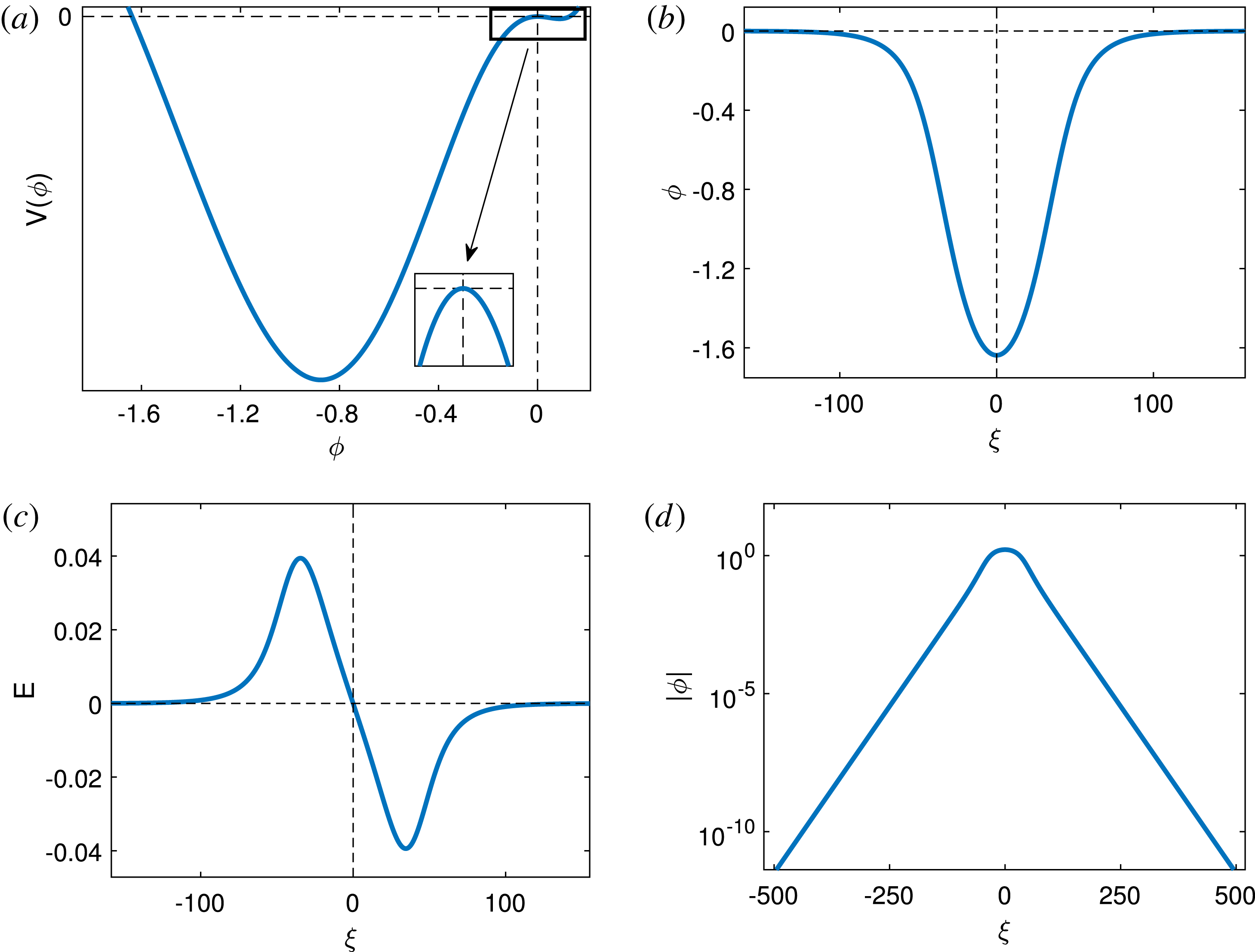
. The Sagdeev potential is shown in (a). In (b) and (c), the electrostatic potential and the electric field of the soliton are shown, respectively. In (d), the absolute value of the electrostatic potential is shown on a logarithmic scale.

We start off by considering a regular soliton. For this, we chose
 $f=0.3$
,
 $\unicode[STIX]{x1D707}=10$
and
 $\unicode[STIX]{x1D6FD}=0.26$
. Figure 4 shows the results for a regular soliton with velocity
 $M=1.003M_{a}\approx 1.4143$
. In figure 4(a) we show the Sagdeev potential. Here the root
 $\unicode[STIX]{x1D719}_{r}\approx -1.638$
gives the amplitude of the soliton. The superimposed figure (indicated with the arrow) shows the same Sagdeev potential in the vicinity of the origin, highlighting that the Sagdeev potential forms a local maximum at the equilibrium
 $\unicode[STIX]{x1D719}=0$
. As a result, the soliton propagates faster than the acoustic speed, so that the approximation (2.4) can be used to estimate the Sagdeev potential near
 $\unicode[STIX]{x1D719}=0$
.
In figure 4(b) we show the typical bell-shaped soliton solution that forms in the electrostatic potential
 $\unicode[STIX]{x1D719}$
. The negative polarity of the soliton means that a dip in the electrostatic potential is observed. In figure 4(c) the typical bipolar electric field
 $E$
associated with a soliton is shown. In order to examine the tails of the soliton, we plot the absolute value of the electrostatic potential
 $|\unicode[STIX]{x1D719}|$
on a logarithmic scale in figure 4(d). Note the symmetry in
 $\unicode[STIX]{x1D709}$
that is characteristic of solitons. On both sides we see that the solution approaches straight lines. The lack of curvature in the tails is associated with the exponential decay rate that was derived in (2.9). The derivatives of the Sagdeev potential show that
 $B\approx -5.2\times 10^{-4}$
.
These results can now be compared to an acoustic speed soliton. To do this, we used the same parameters as above, and considered the acoustic speed
 $M=M_{a}\approx 1.4101$
. In figure 5(a) we show the corresponding Sagdeev potential. The superimposed figure (indicated with the arrow) shows that the Sagdeev potential forms a saddle point at the equilibrium electrostatic potential
 $\unicode[STIX]{x1D719}=0$
. This indicates that the soliton occurs at the acoustic speed. As a result, the Sagdeev potential near the equilibrium electrostatic potential can be approximated by (2.5).
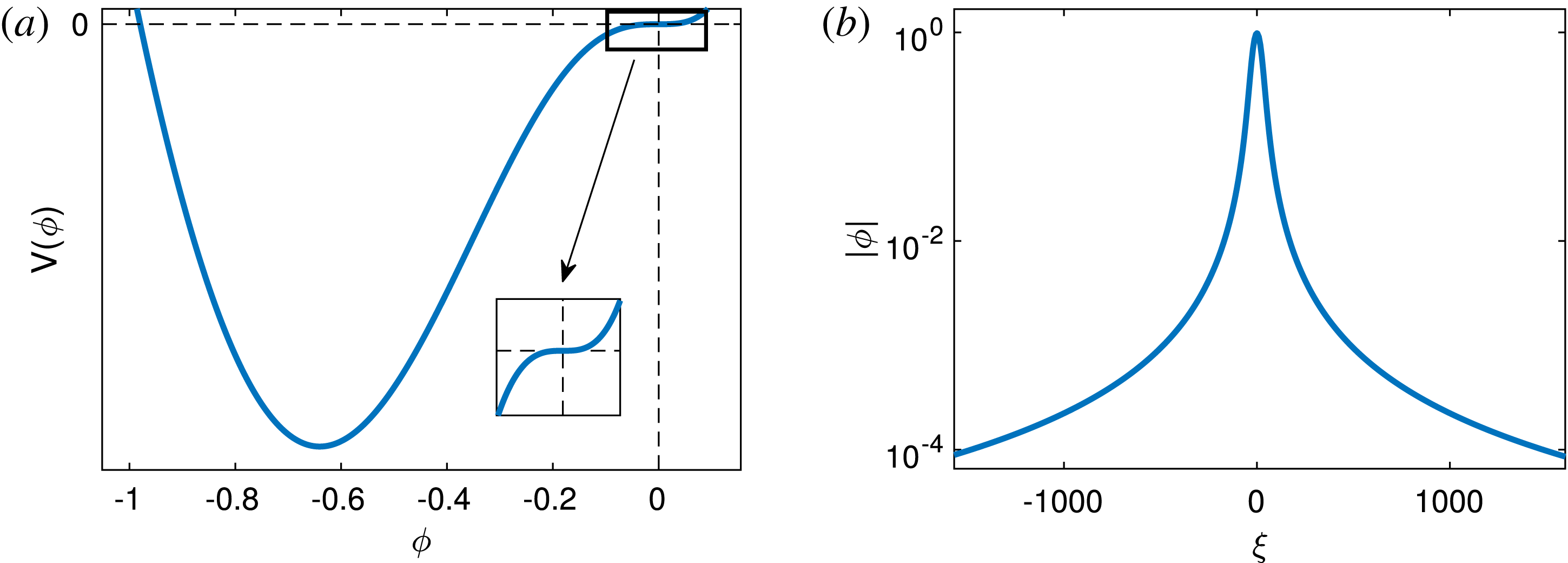
In figure 5(b) we consider the tails of the soliton by plotting the absolute value of the electrostatic potential
 $|\unicode[STIX]{x1D719}|$
on a logarithmic scale. Notice that both tails are concave upwards, a clear indication that the tails decay at the algebraic rate (2.15). From the appropriate derivatives of the Sagdeev potential (4.2) it follows that
 $C=0.0094$
. This is entirely different to the exponential decay observed in the super-acoustic soliton shown in figure 4(d).
Acoustic speed soliton solution for
 $\unicode[STIX]{x1D707}=10$
,
 $\unicode[STIX]{x1D6FD}=0.26$
,
 $f=0.3$
and
 $M=M_{a}\approx 1.4101$
. The Sagdeev potential is shown in (a). In (b) the absolute value of the electrostatic potential is shown on a logarithmic scale.

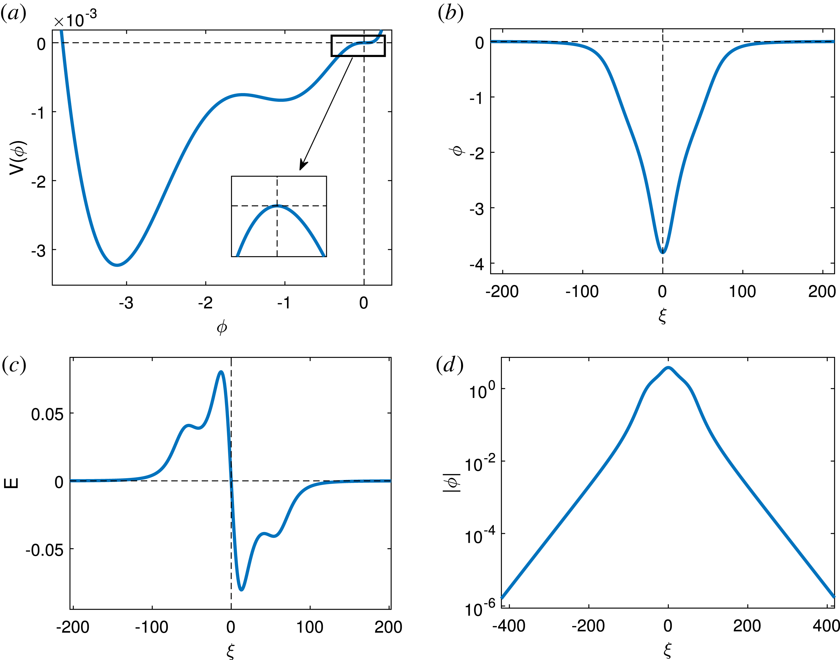
The same principles apply to the difference between acoustic speed supersolitons and regular supersolitons. A supersoliton is a deformed soliton. Unlike the bipolar electric field structure of solitons, supersolitons have three local minima and three local maxima in the electric field. Indeed, the characteristic ‘wiggles’ of the electric field is associated with the core of the supersoliton, and not the tails.
To illustrate this, we use the parameters
 $f=0.293$
,
 $\unicode[STIX]{x1D707}=10$
and
 $\unicode[STIX]{x1D6FD}=0.26$
. We first consider the super-acoustic speed supersoliton that forms at
 $M=1.001M_{a}\approx 1.404$
. In figure 6(a) the Sagdeev potential is shown. Notice that the additional local minimum and local maximum give rise to the supersoliton’s shape. From the superimposed figure (indicated with the arrow), it is clear that the Sagdeev potential forms a local maximum at
 $\unicode[STIX]{x1D719}=0$
.
In figure 6(b) we plot the electrostatic potential
 $\unicode[STIX]{x1D719}$
, showing a deformation in the bell shape that is typical of regular solitons. In figure 6(c) the electric field
 $E$
is shown, where the additional local minima and local maxima can be seen. In figure 6(d) we show the tails of the supersoliton by plotting the absolute value of the electrostatic potential
 $|\unicode[STIX]{x1D719}|$
on a logarithmic scale. Once again, the lack of curvature indicates that the tails decay at an exponential rate described by (2.9) for
 $B\approx -5.2\times 10^{-4}$
.
Regular supersoliton solution for
 $\unicode[STIX]{x1D707}=10$
,
 $\unicode[STIX]{x1D6FD}=0.26$
,
 $f=0.293$
and
 $M=1.001M_{a}\approx 1.404$
. The Sagdeev potential is shown in (a). In (b) and (c), the electrostatic potential and the electric field of the soliton are shown, respectively. In (d) the absolute value of the electrostatic potential is shown on a logarithmic scale.

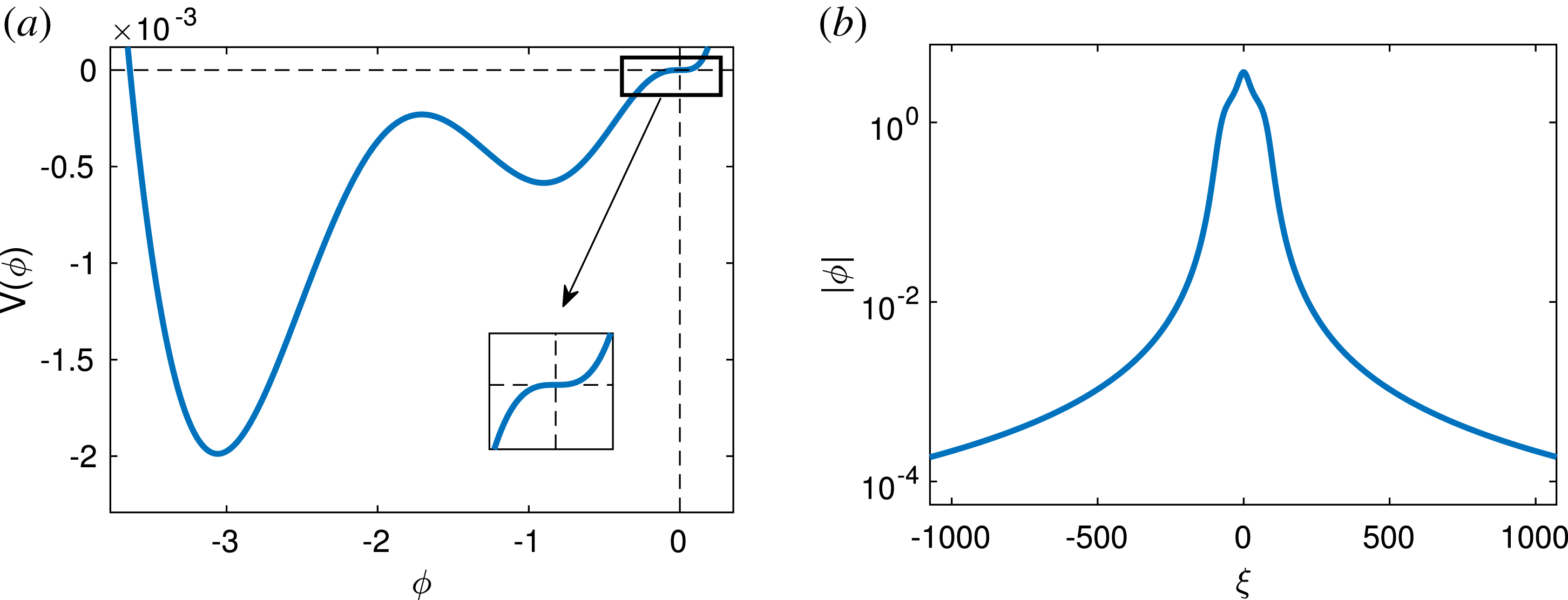
For the chosen parameters, one also finds an acoustic speed supersoliton at
 $M=M_{a}\approx 1.4026$
. In figure 7(a) the Sagdeev potential is shown. Notice the saddle point at the equilibrium
 $\unicode[STIX]{x1D719}=0$
, that is clearly seen on the superimposed plot (indicated with the arrow). This indicates the acoustic speed nature of the supersoliton. In figure 7(b) the tails of the supersoliton are shown. Once again, the concave upward nature of these tails indicates the algebraic decay rate, given by (2.15) with
 $C\approx 0.011$
.
Acoustic speed supersoliton solution for
 $\unicode[STIX]{x1D707}=10$
,
 $\unicode[STIX]{x1D6FD}=0.26$
,
 $f=0.293$
and
 $M=M_{a}\approx 1.4026$
. The Sagdeev potential is shown in (a). In (b) the absolute value of the electrostatic potential is shown on a logarithmic scale.

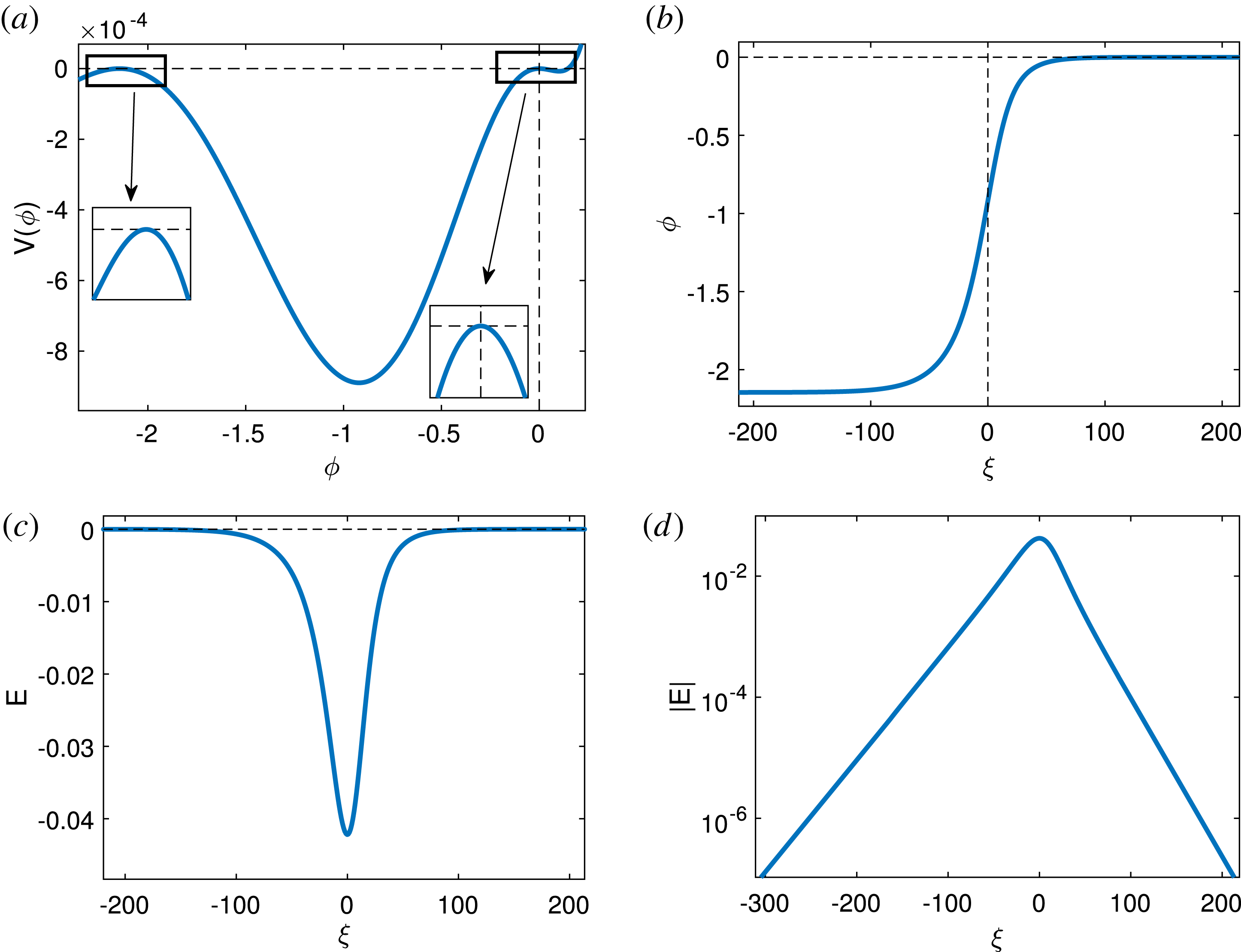
We now turn our attention to double layers. To start off, we consider a regular double layer. By regular double layer, we mean that it propagates faster than the acoustic speed, and that it is not associated with a triple root. Here we choose
 $f=0.3$
,
 $\unicode[STIX]{x1D707}=10$
and
 $\unicode[STIX]{x1D6FD}=0.26$
. For these parameters, the double layer arises at the velocity
 $M_{DL}\approx 1.415$
. The results are shown in figure 8. In figure 8(a) the Sagdeev potential is shown. Here we superimposed two figures, indicated with arrows. The arrows on the right- and left-hand sides show the Sagdeev potential in the vicinity of the origin
 $\unicode[STIX]{x1D719}=0$
and in the vicinity of the double layer root
 $\unicode[STIX]{x1D719}_{DL}$
, respectively. In both cases, we see that a local maximum forms.
The electrostatic potential
 $\unicode[STIX]{x1D719}$
of the double layer is shown in figure 8(b). Here the two layers of the double layer can be clearly seen. In figure 8(c) the electric field
 $E$
of the double layer is shown to form a bell-shaped structure with negative polarity. To show the tails of the double layer, we plot the absolute value of the electrostatic potential
 $|E|$
on a logarithmic scale in figure 8(d). We can see that both tails have no curvature, indicating exponential decay.
Regular double layer solution for
 $\unicode[STIX]{x1D707}=10$
,
 $\unicode[STIX]{x1D6FD}=0.26$
,
 $f=0.3$
and
 $M=M_{DL}\approx 1.415$
. The Sagdeev potential is shown in (a). In (b) and (c), the electrostatic potential and the electric field of the soliton are shown, respectively. In (d) the absolute value of the electric field is shown on a logarithmic scale.

It should be noted that the two tails have different decaying rates. This is due to the fact that the electrostatic potential
 $\unicode[STIX]{x1D719}$
of the tail on the left-hand side is governed by (3.7). Since
 $$\begin{eqnarray}E=-\unicode[STIX]{x1D735}\unicode[STIX]{x1D719},\end{eqnarray}$$
it follows directly that
 $$\begin{eqnarray}E\propto \exp \left(\sqrt{-2B_{DL}}\unicode[STIX]{x1D709}\right)\end{eqnarray}$$
when
 $\unicode[STIX]{x1D709}\rightarrow -\infty$
. On the other hand, the electrostatic potential
 $\unicode[STIX]{x1D719}$
of the tail on the right-hand side is governed by (3.1). From (4.4) it follows that
 $$\begin{eqnarray}E\propto \exp \left(\sqrt{-2B}\unicode[STIX]{x1D709}\right),\end{eqnarray}$$
when
 $\unicode[STIX]{x1D709}\rightarrow +\infty$
. For the chosen parameters, we have
 $B=-0.0018$
and
 $B_{DL}\approx B/2$
. As a result, the left-hand side of the tail decays much slower than the right-hand side. This difference gives rise to the asymmetry shown in figure 8(d).
We now consider an acoustic speed double layer. We found this when the parameters are chosen as follows:
 $\unicode[STIX]{x1D707}=10$
,
 $\unicode[STIX]{x1D6FD}=0.26$
,
 $f\approx 0.29376$
and
 $M=M_{a}\approx 1.403$
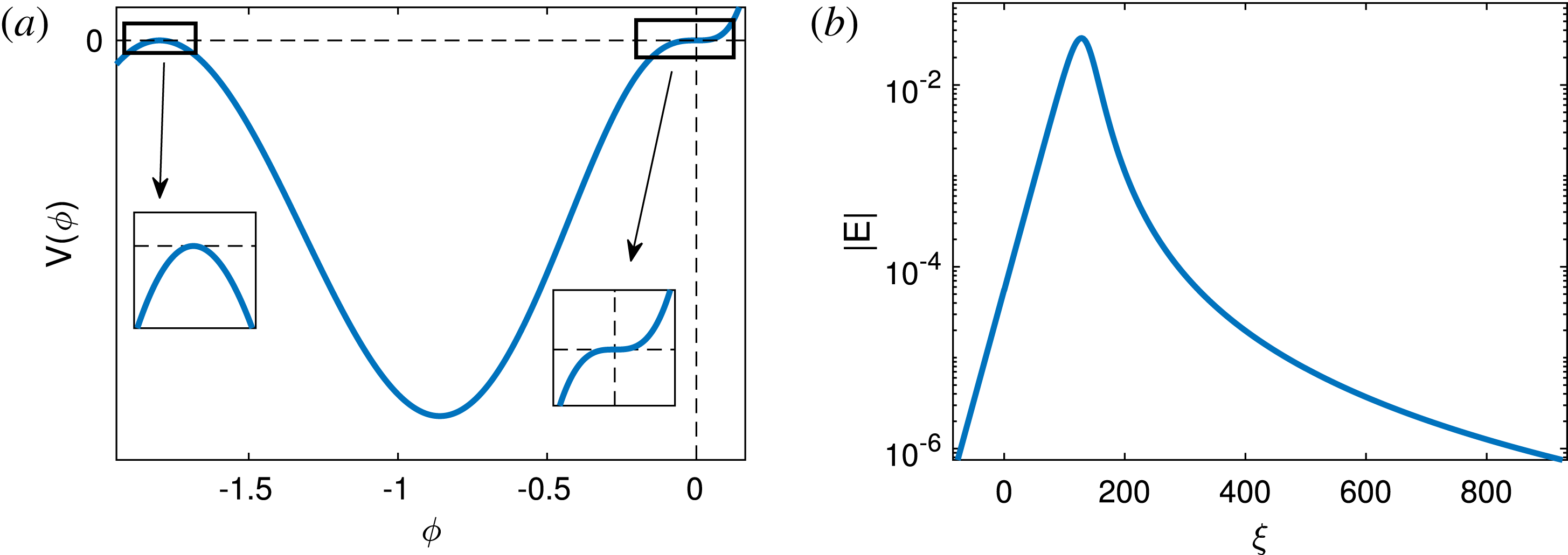
. The Sagdeev potential is shown in figure 9(a). One of the superimposed figures (indicated with the arrow on the left-hand side) shows that a local maximum forms at the root
 $\unicode[STIX]{x1D719}_{DL}\approx -1.798$
. The other superimposed figure (indicated with the arrow on the right-hand side) shows that a saddle point forms at the origin
 $\unicode[STIX]{x1D719}=0$
.
In figure 9(b) the absolute value of the electric field
 $|E|$
is plotted on a logarithmic scale. Here we see that the tail on the left-hand side decays much faster. The lack of curvature indicates that the solution decays at an exponential rate. Indeed, from the asymptotic analysis it follows that the tail decays at the exponential rate according to (4.5) when
 $\unicode[STIX]{x1D709}\rightarrow -\infty$
. On the other hand, the tail on the right-hand side is concave upwards, corresponding to algebraic decay. From (3.2) and (4.4) it follows that
 $$\begin{eqnarray}E\rightarrow -\frac{4}{C(\unicode[STIX]{x1D709}-\unicode[STIX]{x1D709}_{0})^{3}}\end{eqnarray}$$
when
 $\unicode[STIX]{x1D709}\rightarrow +\infty$
. Therefore, the behaviour of the two tails are very different.
Acoustic speed double layer solution for
 $\unicode[STIX]{x1D707}=10$
,
 $\unicode[STIX]{x1D6FD}=0.26$
,
 $f\approx 0.29376$
and
 $M=M_{a}\approx 1.403$
. The Sagdeev potential is shown in (a). In (b), the absolute value of the electric field is shown on a logarithmic scale.

We next consider double layers associated with a triple root. To start off, we consider a double layer with a triple root that propagates faster than the acoustic speed. We found such a structure at parameters
 $\unicode[STIX]{x1D707}=10$
,
 $\unicode[STIX]{x1D6FD}=0.26$
,
 $f\approx 0.3015$
and
 $M_{DL}\approx 1.412$
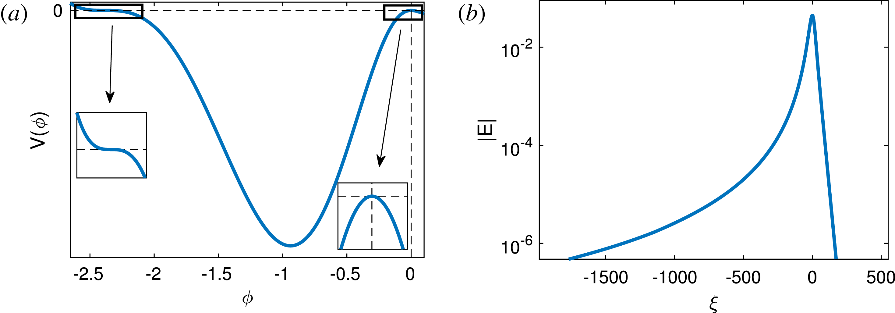
. The Sagdeev potential is shown in figure 10(a). The superimposed figure indicated with the arrow on the left-hand side shows that the root
 $\unicode[STIX]{x1D719}_{DL}\approx -2.389$
forms a saddle point on the
 $\unicode[STIX]{x1D719}$
-axis, so that a triple root arises. On the other hand, the superimposed figure indicated with the arrow on the right-hand side shows that a local maximum forms at the origin. This is associated with double layers moving faster than the acoustic speed.
The tails of the double layer are shown in figure 10(b) by plotting the absolute value of the electric field
 $|E|$
on a logarithmic scale. In this case, the tail on the right-hand side decays exponentially fast according to (4.6) due to the non-zero coefficient
 $B\approx -0.0023$
. On the other hand, the upward concavity of the tail on the left-hand side indicates algebraic decay. This is due to the fact that
 $B_{DL}=0$
. In the limit
 $\unicode[STIX]{x1D709}\rightarrow -\infty$
, it follows from (3.9) and (4.4) that
 $$\begin{eqnarray}E\rightarrow -\frac{4}{C_{DL}(\unicode[STIX]{x1D709}-\unicode[STIX]{x1D709}_{0})^{3}}.\end{eqnarray}$$
Double layer solution associated with a triple root for
 $\unicode[STIX]{x1D707}=10$
,
 $\unicode[STIX]{x1D6FD}=0.26$
,
 $f\approx 0.3015$
and
 $M=M_{DL}\approx 1.412$
. The Sagdeev potential is shown in (a). In (b), the absolute value of the electric field is shown on a logarithmic scale.

Finally, we show the special case of an acoustic speed double layer with a triple root. For this, we chose
 $\unicode[STIX]{x1D707}=10$
,
 $\unicode[STIX]{x1D6FD}\approx 0.2548$
,
 $f\approx 0.2991$
with acoustic speed
 $M_{a}\approx 1.4042$
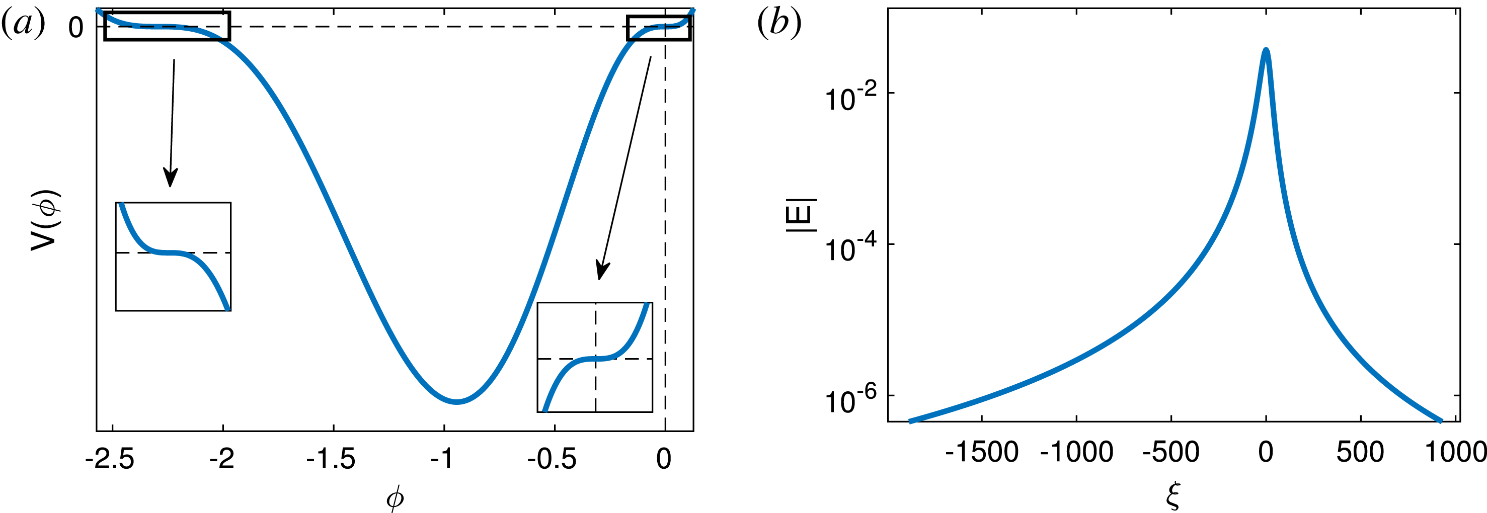
. In figure 11(a) the Sagdeev potential is shown for the chosen parameters. The superimposed figures show that both the root
 $\unicode[STIX]{x1D719}_{DL}$
(arrow on the left-hand side) and the origin
 $\unicode[STIX]{x1D719}=0$
(arrow on the right-hand side) form saddle points. In figure 11(b) the absolute value of the electric field
 $|E|$
is shown on a logarithmic scale. In this case, we see that both tails are concave upwards, corresponding to algebraic decay. Once again, one can observe a clear asymmetry in the decay rates. This is due to the fact that the tail on the left-hand side decays according to (4.8), whereas the tail on the right-hand side decays according to (4.7). Since
 $C_{DL}\approx -0.0013$
is much smaller (in absolute terms) than
 $C\approx 0.0114$
, it follows that the tail on the left-hand side decays slower than the tail on the right-hand side.
Acoustic speed double layer solution associated with a triple root for
 $\unicode[STIX]{x1D707}=10$
,
 $\unicode[STIX]{x1D6FD}\approx 0.2548$
,
 $f\approx 0.2991$
and
 $M=M_{a}\approx 1.4042$
. The Sagdeev potential is shown in (a). In (b) the absolute value of the electric field is shown on a logarithmic scale.

5 Conclusions
In this paper we examined the asymptotic behaviour of acoustic speed solitons and double layers. This was performed by applying a Taylor series expansion to the Sagdeev pseudopotential function.
The results show that the decay rate of the electrostatic potential of acoustic speed solitons can be described by a power law. This algebraic rate of decay is much slower than the exponential decay rate associated with solitons that propagate faster than the acoustic speed.
We also considered acoustic speed double layers. We showed that the decay rate of one of the tails of the associated electric field decays according to a power law. This is also much slower than the exponential rate of decay associated with double layers that propagate faster than the acoustic speed.
The asymptotic behaviour of the other side of the electric field tail associated with double layers was also studied. The study shows that the decay rate can be obtained by applying a Taylor series expansion to the double layer root. It follows that this tail decays exponentially fast whenever a double root (i.e. local maximum) forms, while it decays only algebraically fast whenever the Sagdeev potential forms a triple root, i.e. a saddle point on the
 $\unicode[STIX]{x1D719}$
-axis.
The results are illustrated through a case study of plasmas consisting of two oppositely charged cold ion species with Cairns-distributed electrons. The case study shows that the results for acoustic speed solitons also apply to acoustic speed supersolitons. These characteristics may be useful for identifying acoustic speed solitons and double layers in space and laboratory plasmas.
Acknowledgements
C.P.O. wishes to acknowledge the financial assistance of the National Research Foundation (NRF) towards this research. Opinions expressed and conclusions arrived at, are those of the authors and are not necessarily to be attributed to the NRF.