1 Introduction
Plasmas are ubiquitous in the Universe, and host a number of processes that regulate the physics of many astrophysical bodies, including nuclear fusion. Artificial plasmas created in the laboratory have played a fundamental role in the development of modern physics, by providing laboratory-controlled environments in which theories could be tested, experiments could be carried out, and atomic and plasma parameters could be measured. Over the years, several devices and techniques have been developed to produce and maintain, under controlled conditions, various types of plasmas: gas discharge plasmas, laser-produced plasmas,  $Z$-pinch plasmas and magnetic confined plasmas. Very recently, plasmas have found applications, even far from scientific laboratories, in industrial production and medicine, opening new perspectives and requiring new solutions.
The measurement of the physical properties of plasmas is of critical importance for understanding, monitoring and controlling the conditions created inside a laboratory plasma chamber, as well as determining the presence and amount of impurities. For example, a complete knowledge of the plasma properties inside an electron cyclotron resonance ion source (known as ECRIS, Geller (Reference Geller1976)), commonly employed to feed particle accelerators, will provide the key for a better comprehension of plasma formation and heating required to fully control the ion flows, currently optimized by adopting approximate semiempirical relations.
Among the laboratory plasma diagnostics, emission spectroscopy (ES) in the X-ray and visible ranges has been widely applied thanks to its being a non-invasive method which leaves the plasma to be studied unperturbed. At typical low resolution of  $R = \lambda /\varDelta \lambda \sim 10^{2\div 3}$, ES is mainly limited to characterize the electron component of plasmas. The building of a new generation of instruments with very high resolution in the visible (3000–8000 Å,
 $R \sim 10^4$; Kronholm et al. (Reference Kronholm, Kalvas, Koivisto, Kosonen, Marttinen, Neben, Sakildien, Tarvainen and Toivanen2020)), UV (700–4000 Å,
 $R \sim 10^4$; Giarrusso et al. (Reference Kronholm, Kalvas, Koivisto, Kosonen, Marttinen, Neben, Sakildien, Tarvainen and Toivanen2020)) and in the X-ray domain (0.2–12 keV,
 $R \sim 10^3$; Barret et al. (Reference Barret, Lam Trong, den Herder, Piro, Barcons, Huovelin, Kelley, Mas-Hesse, Mitsuda and Paltani2016)) allows the application of ES to the analysis of spectral line profiles deriving further plasma quantities and atomic data. In Giarrusso et al. (Reference Giarrusso, Avila, Del Zanna, Landi, Leone, Munari, Castro, Celona, Gammino and Mascali2018) we discussed (i) the importance of high-resolution spectropolarimetry to correctly interpret the non-isotropic spectral emission signed by the presence of confining or self-induced magnetic fields (Fujimoto & Iwamae Reference Fujimoto and Iwamae2008); and (ii) the advantage of échelle spectrographs, able to cover in a single exposure a very large wavelength range (3700–11 000 Å, Leone et al. (Reference Leone, Avila, Bellassai, Bruno, Catalano, Di Benedetto, Di Stefano, Gangi, Giarrusso and Greco2016)), as opposed to monochromators (Kronholm et al. Reference Kronholm, Kalvas, Koivisto, Kosonen, Marttinen, Neben, Sakildien, Tarvainen and Toivanen2020) which are able to cover a few hundred Å wavelength interval if equipped with two-dimensional detectors.
However, the diagnostic use of these high-resolution spectra requires the availability of an unprecedented amount of high-accuracy atomic data, transition rates and software that allow us to predict plasma emission as a function of the relevant plasma parameters. In addition, as laboratory plasmas are strongly magnetized, accurate measurements of the magnetic field strength and orientation are also required to fully characterize and control the plasma status, as well as to correctly interpret the plasma emission.
In response to this need, several spectral codes have been developed to provide the data and software to calculate emissivities from optically thin plasmas, e.g. the atomic data and analysis structure (ADAS, Summers (Reference Summers2004)), FLYCHK (Chung et al. Reference Chung, Chen, Morgan, Ralchenko and Lee2005), AtomDB (Smith et al. Reference Smith, Brickhouse, Liedahl and Raymond2001), SPEX (Kaastra, Mewe & Nieuwenhuijzen Reference Kaastra, Mewe, Nieuwenhuijzen, Yamashita and Watanabe1996) and CHIANTI (Dere et al. Reference Dere, Landi, Mason, Monsignori Fossi and Young1997, Reference Dere, Del Zanna, Young, Landi and Sutherland2019). While not complete, each of these spectral codes provides both the atomic data and the radiative and collision rates necessary to calculate plasma emissivities for a number of ions of many elements, as well as software to perform the calculations, interact with the atomic data and carry out plasma diagnostics.
In the present work we aim at upgrading the CHIANTI spectral code with software programs able to predict the spectral signatures of the Zeeman effect as a function of magnetic field magnitude and orientation (inclination angle and azimuth) relative to the line of sight (i.e. the direction of spectra acquisition), providing the emissivities in all four Stokes parameters. We chose to upgrade CHIANTI because of its completeness, free availability and its frequent upgrades that allow this code to include the most up-to-date atomic data and transition rates available in the literature in a timely manner.
In § 2 we summarize the main features of the CHIANTI spectral code, in § 3 we describe how Zeeman splitting has been implemented in CHIANTI and in § 4 we present examples of CHIANTI synthetic spectra to show the magnetic field diagnostic possibilities provided by this update.
2 The CHIANTI spectral code
The CHIANTI spectral code consists of a database of atomic data and transition probabilities and a suite of computer programs, which allow one to calculate the emissivity of optically thin plasmas in the 0.01–1000 MK temperature range (approximately 1 eV to  ${\approx }$80 keV) and to carry out spectroscopic diagnostics from optically thin spectra. First released in 1997 (Dere et al. Reference Dere, Landi, Mason, Monsignori Fossi and Young1997), CHIANTI has been primarily designed to analyse the emission of solar and solar-like stellar upper atmospheres, under the assumption of optically thin plasmas. Since its first release, CHIANTI has undergone eight major upgrades, the most recent of which was in 2019 (Dere et al. Reference Dere, Del Zanna, Young, Landi and Sutherland2019), and its applications have gone far beyond the boundaries of the physics of the solar and stellar upper atmospheres. In fact, CHIANTI software and data have been applied to all astrophysical plasmas found in objects ranging from comets to galaxies, as well as to laboratory plasmas. The code is optimized for spectral range 1–2000 Å, but data are available to calculate line and continuum emission from solar and stellar atmospheric plasmas also at visible and infrared wavelengths.
The CHIANTI atomic database includes data for almost all the ions of the elements lighter than Zn (atomic number  $Z\leq 30$). Special care has been placed in multiply ionized systems, as these are the ones that emit the bulk of the lines populating solar and stellar spectra. The data included in CHIANTI consist of energy levels, atomic level identification parameters, Einstein coefficients for spontaneous emission, as well as electron–ion collisional excitation rate coefficients. Also, data to calculate satellite line emission is included. Proton–ion excitation rate coefficients are also included for a number of important ions. Photoexcitation from a background source can also be taken into account in the calculations.
Originally, line emission was computed in CHIANTI by evaluating the level populations of emitting ions under the Collisional-Radiative model. However, very soon the availability of calculations providing electron–ion excitation rate coefficients and Einstein coefficients for transitions between levels in excited configurations has allowed the code to include electron–ion excitation between highly excited levels, as well as radiative cascades, extending the validity of CHIANTI emissivities to density ranges suitable for laboratory plasmas.
Data and software to calculate continuum Bremsstrahlung, free-bound and two-photon emission from all the ions in the database are included, and they are particularly important for the X-ray range.
The CHIANTI spectral code also includes a complete database of ionization and recombination rates for all the elements between H and Zn. The processes taken into account are direct collisional ionization, excitation–autoionization, radiative recombination and dielectronic recombination. Due to its focus on coronal plasmas, where charge exchange phenomena are negligible, this process is not included. Also, photoionization from a background source is not included. Thus, while the CHIANTI software calculates line emissivities assuming ionization equilibrium, data are available to model time-dependent ionization.
The CHIANTI software consists of tools that allow one to calculate line and continuum emission with user-defined electron densities and temperatures of isothermal plasmas; in case of multithermal plasmas CHIANTI allows users to carry out calculations at constant pressure or through a user-provided plasma distribution with temperature (e.g. the differential emission measure (DEM)). The plasma chemical composition can be either chosen by the user from a number of different sets provided by the team (that describe different sets of solar photospheric or coronal abundances), or directly provided by the user through a simple ASCII file, which makes it easy to adapt CHIANTI calculations to any type of laboratory plasma composition. Also, a suite of programs to analyse data and measure the plasma electron temperature, electron density and DEM is included in CHIANTI.
All CHIANTI calculations are carried out neglecting the effects of the magnetic field; in this work, we introduce spectral line splitting due to the Zeeman effect.
3 Introducing the Zeeman splitting in CHIANTI
Spectra from magnetized plasma need to be analysed by taking into account the effect of the magnetic field  $\boldsymbol {B}$, which removes the degeneracy of atomic energy levels. Indeed the presence of
 ${\boldsymbol {B}}$ lets each atomic level (described by the total angular momentum
 $J$, the total orbital angular momentum
 $L$ and the total spin angular momentum
 $S$) split into
 $2J+1$ sublevels identified by the magnetic quantum number
 $M_J$ (which ranges from
 $-J$ to
 $+J$). As a consequence, if the field intensity is weaker than the internal atomic one, spectral lines usually split into a series of Zeeman components. Under the L-S coupling scheme, using subscript u and d to refer to the upper and lower level of the transition, respectively, the Zeeman components are called
 ${\rm \pi}$ components when
 ${\rm \Delta} M = M_{J_{u}} - M_{J_{d}} = 0$, blue-shifted components
 $\sigma _{b}$ for
 ${\rm \Delta} M = +1$ and red-shifted components
 $\sigma _{r}$ for
 ${\rm \Delta} M = -1$ (see Landi Degl'Innocenti & Landolfi (Reference Landi Degl'Innocenti and Landolfi2004), for details).
Furthermore, when a magnetic field  ${\boldsymbol {B}}$ is present the emission is not isotropic, i.e. the strength and shape of spectral lines depend on the magnetic field orientation with respect to the line of sight. As reported in Giarrusso (Reference Giarrusso2019), Zeeman
 ${\rm \pi}$ components, always linearly polarized along the magnetic field direction, are absent when observed along
 ${\boldsymbol {B}}$ and reach their maximum intensity when observed perpendicularly to the field. Zeeman
 $\sigma$ components are circularly polarized (reaching their maximum intensity) when observed along the field, and are linearly polarized (reaching their minimum intensity) when observed perpendicularly to
 ${\boldsymbol {B}}$, and are elliptically polarized when observed at an arbitrary angle with respect to
 ${\boldsymbol {B}}$. So, synthetic spectra for plasma diagnostics need to take into account not only the magnitude
 $|{\boldsymbol {B}}|$ of the field, but also the value of inclination angle (
 $\theta$) and azimuth (
 $\chi$) of
 ${\boldsymbol {B}}$ with respect to the line of sight.
Polarization can be described through the Stokes parameters  $I$,
 $Q$,
 $U$,
 $V$. Stokes
 $I$ represents the sum of the intensities of the observed Zeeman components. In the following, Stokes
 $Q$ is related to the linear polarization degree in the direction parallel and perpendicular to
 ${\boldsymbol {B}}$, Stokes
 $U$ refers to linear polarization at
 ${\pm }45^{\circ }$ with respect to the field direction and Stokes
 $V$ indicates the circular polarization. The signs of
 $Q$,
 $U$ and
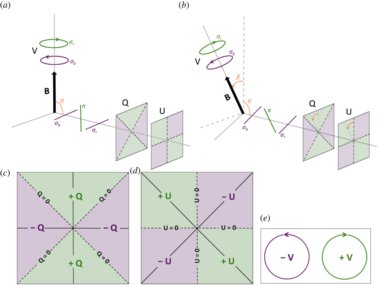
 $V$ are shown in figure 1. If the instrument's spectral resolution is not high enough to resolve the individual Zeeman components, the measurement of the Stokes parameters obtained through a polarimeter provides tools to reconstruct the field's strength and orientation as well as to correctly interpret the observed spectrum.
(c,d,e) Definition of Stokes  $Q$,
 $U$ and
 $V$ signs. (a,b) Signs of Stokes
 $Q$,
 $U$ and
 $V$, for emission detected along the field direction (
 $\theta = 0^{\circ }$,
 $\chi$ undefined) and orthogonally to the magnetic field (
 $\theta = 90^{\circ }$) for
 $\chi = 0^{\circ }$ (a) and
 $\chi > 0^{\circ }$ (b).

The introduction of Zeeman splitting in CHIANTI (version 8, Del Zanna et al. (Reference Del Zanna, Dere, Young, Landi and Mason2015)) is based on equations reported in Landi Degl'Innocenti & Landolfi (Reference Landi Degl'Innocenti and Landolfi2004). By fixing a value of  $|{\boldsymbol {B}}|$ (expressed in
 $G$),
 $\theta$ and
 $\chi$ (both in degrees), the procedure determines the wavelength
 $\lambda$ and the intensity
 $\mathscr {I}$ of each Zeeman components, as well as the Stokes parameters. First, the Landé
 $g$-factors of the two levels
 \begin{equation} g = 1 + \frac{J (J + 1) + S (S + 1) - L (L + 1)}{2 J (J + 1)} \end{equation}
and the  $M_J$-values of the (
 $2J+1$) different sublevels are derived. Results are combined with the Larmor frequency
 $\nu _{L}$ to determine
 \begin{equation} \lambda = \lambda_{0} - \lambda_{0}^{2} \,\frac{\nu_{L}}{c} (g_{u}M_{J_{u}} - g_{d}M_{J_{d}}), \end{equation}
where  $\lambda _{0}$ is the rest wavelength of the line in the absence of magnetic field and
 $c$ is the speed of light.
The intensity of each Zeeman component integrated over the solid angle is
 \begin{equation} \mathscr{I} = S^{J_{d}J_{u}}_{q}(M_{J_{d}},M_{J_{u}}) \,\mathscr{I}_{{0}} = 3 \begin{pmatrix} J_{u} & J_{d} & 1\\ -M_{J_{u}} & M_{J_{d}} & -q\end{pmatrix}^{2}\,\mathscr{I}_{0}, \end{equation}
where  $\mathscr {I}_{0}$ represents the intensity of the unsplitted line given by CHIANTI in absence of
 ${\boldsymbol {B}}$ and
 $S^{J_{d}J_{u}}_{q}(M_{J_{d}},M_{J_{u}})$ is the relative strength of the component, with
 $q = -{\rm \Delta} M$ equal to
 $-1, 0, +1$ for
 $\sigma _{b}$,
 ${\rm \pi}$,
 $\sigma _{r}$, respectively. The matrix represents the 3-j symbol (Messiah (Reference Messiah1962); Shore & Menzel (Reference Shore and Menzel1968), see appendix A).
The quantities  $\mathscr {I}_{{\rm \pi} }$,
 $\mathscr {I}_{\sigma _{b}}$ and
 $\mathscr {I}_{\sigma _{r}}$ allow us to derive the emissivity in Stokes parameters
 \begin{gather} I = \frac{1}{2} \left[\mathscr{I}_{{\rm \pi}} \sin^2\theta + \frac{\mathscr{I}_{\sigma_{b}} + \mathscr{I}_{\sigma_{r}}}{2} (1 + \cos^2\theta) \right], \end{gather}
 \begin{gather}Q = \frac{1}{2} \left[\mathscr{I}_{{\rm \pi}} - \frac{\mathscr{I}_{\sigma_{b}} + \mathscr{I}_{\sigma_{r}}}{2} \right] \sin^2\theta \cos(2\chi), \end{gather}
 \begin{gather}U = \frac{1}{2} \left[\mathscr{I}_{{\rm \pi}} - \frac{\mathscr{I}_{\sigma_{b}} + \mathscr{I}_{\sigma_{r}}}{2} \right] \sin^2\theta \sin(2\chi), \end{gather}
 \begin{gather}V = \tfrac{1}{2} \left[\mathscr{I}_{\sigma_{r}} - \mathscr{I}_{\sigma_{b}} \right] \cos\theta. \end{gather}
4 Example
As examples of the CHIANTI output, we here discuss a case in the visible range, i.e. the iron line Fe XXIV  $\lambda _{0} = 8194.0889$ Å from the transition
 $1s^2\,6s\,^2S_{1/2} - 1s^2\,6p\,^2P_{3/2}$, as well as the UV emission of the iron line Fe X
 $\lambda _{0} = 1689.0179$ Å from the transition
 $3s^2\,3p\,^4\,3d\,^4F_{5/2} - 3s^2\,3p\,^4\,3d\,^2F_{7/2}$. For both we calculated the line profiles in isothermal approximation for electronic temperature
 $T_{e} = 10^{7}$ K and with constant electronic density
 $N_{e} = 10^{10}\, \textrm {cm}^{-3}$.
For the Fe XXIV line, by setting  $|{\boldsymbol {B}}| = 5$ T we first computed a spectrum along the field direction (
 $\theta = 0^{\circ }$,
 $\chi$ is undefined) (case a), and spectra with null azimuth angle (
 $\chi = 0^{\circ }$) at
 $\theta = 45^{\circ }$ with respect to
 ${\boldsymbol {B}}$ (case b) and perpendicularly to the field (
 $\theta = 90^{\circ }$) (case c). Finally we calculated the spectrum for an arbitrary orientation of the field with respect to the line of sight, i.e.
 $\theta = 30^{\circ }$ and
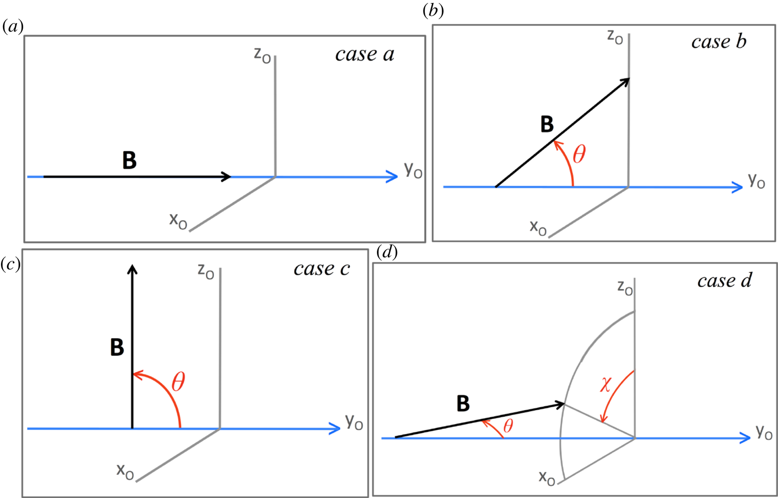
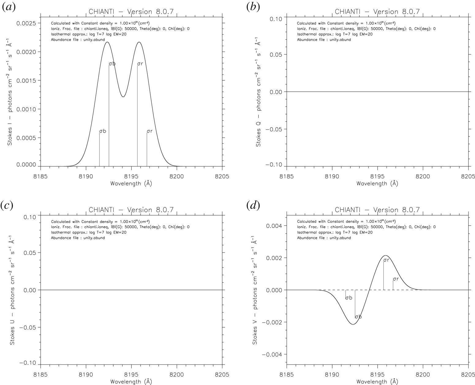
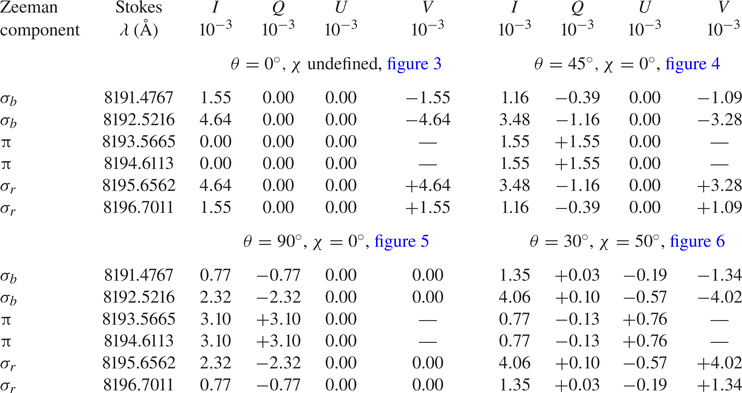
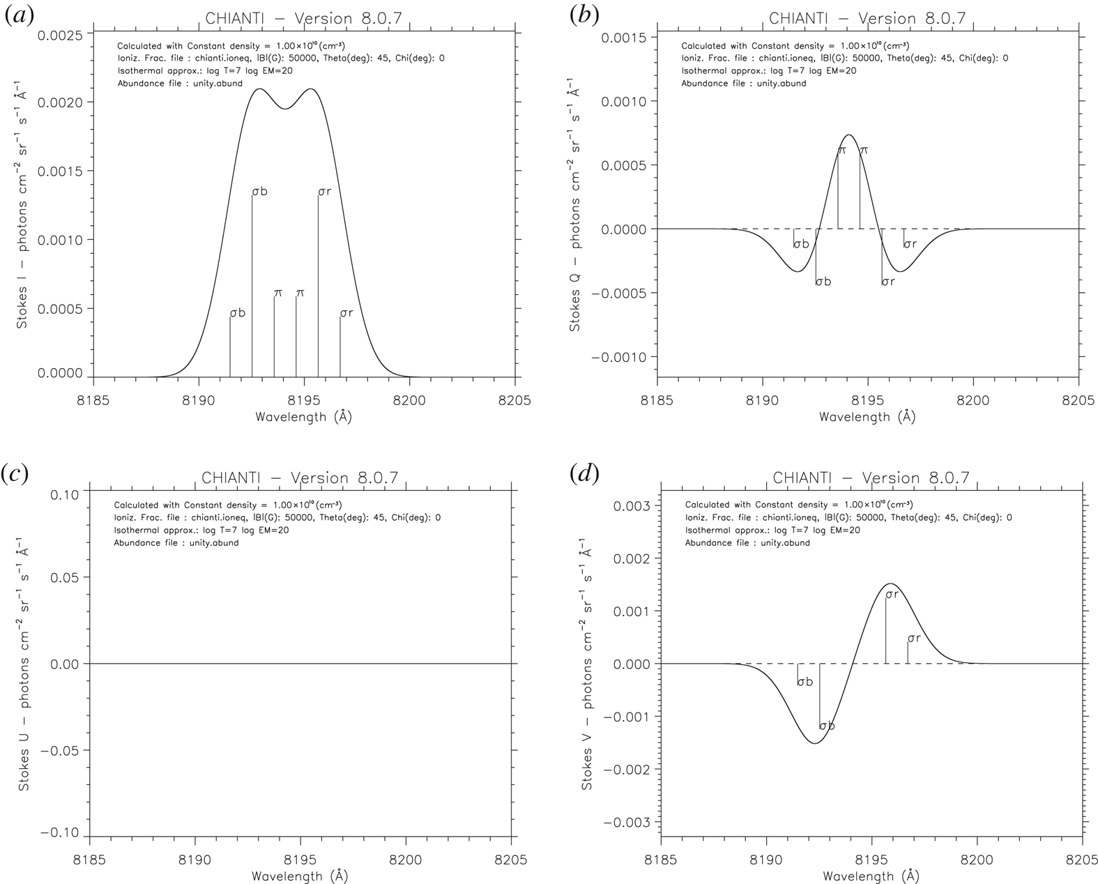
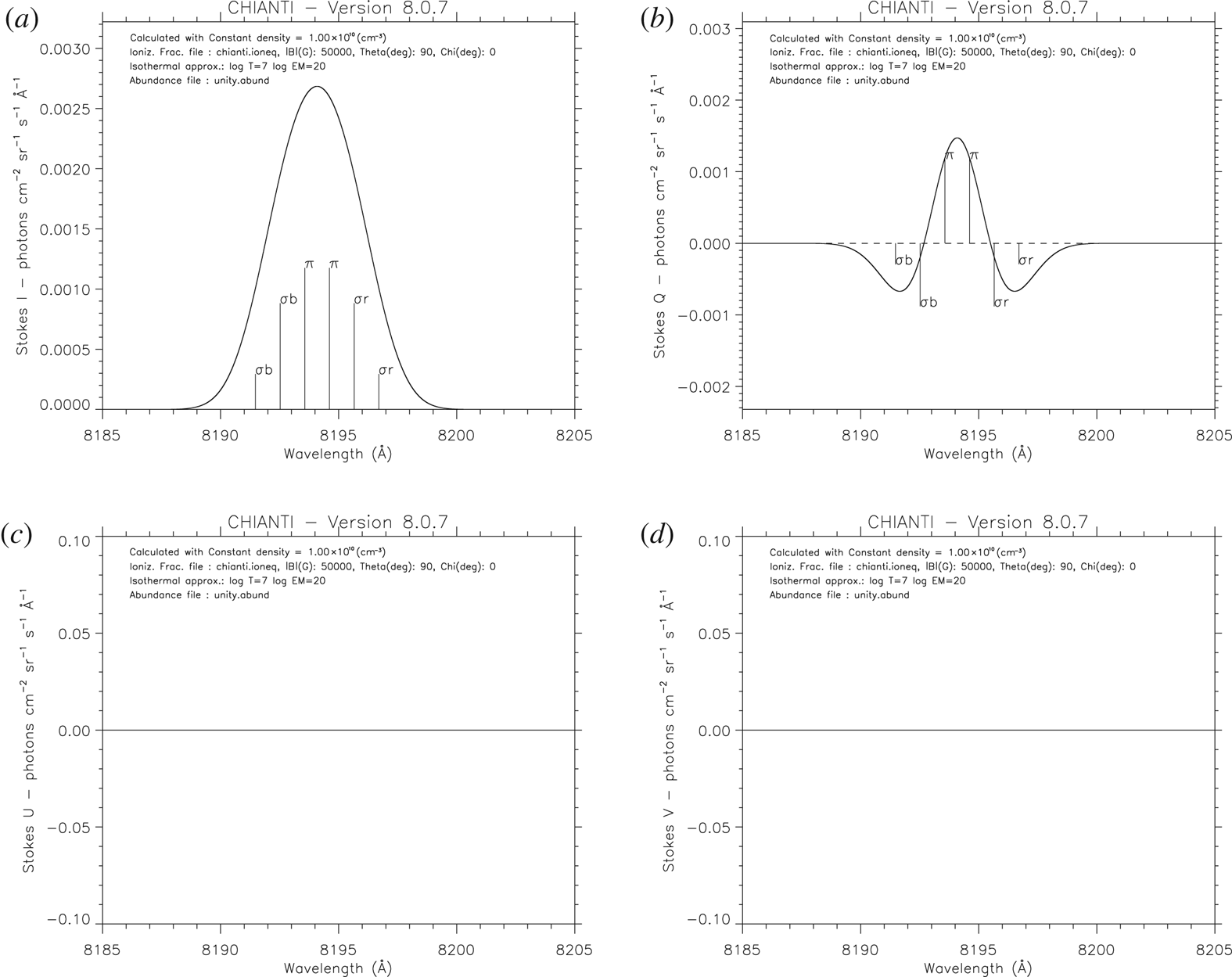
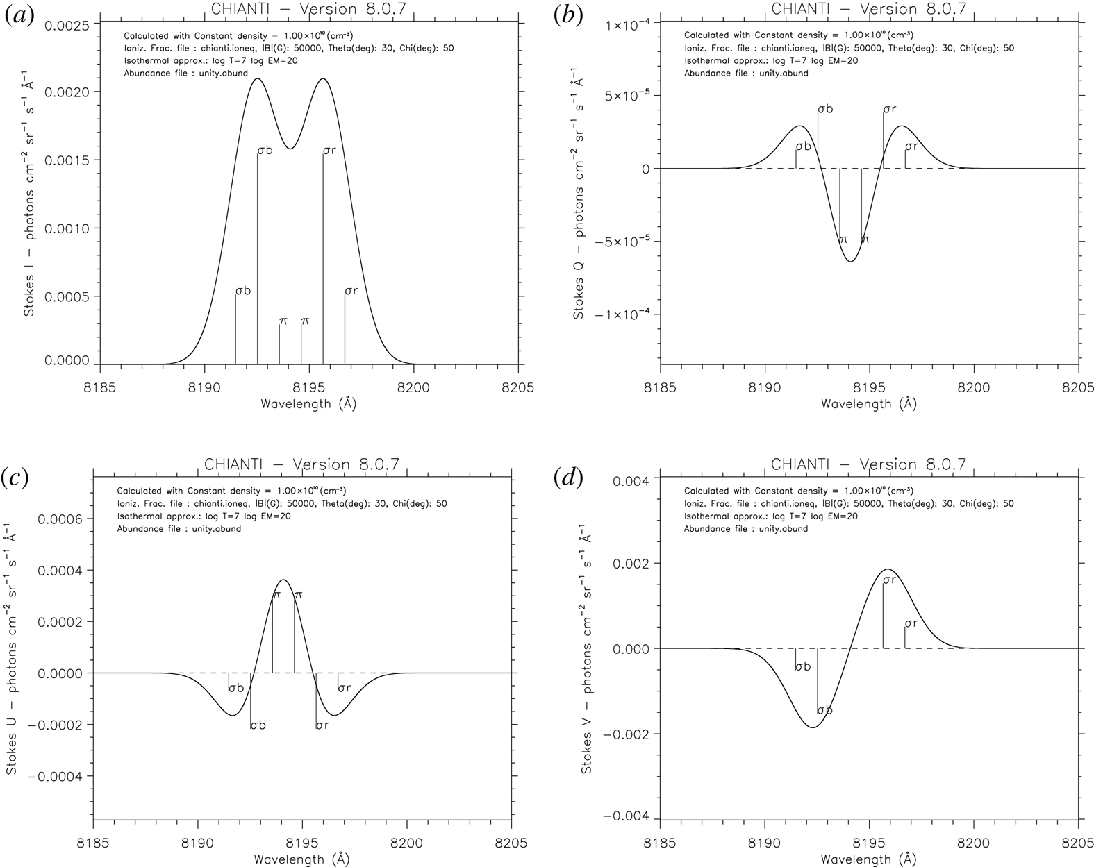
 $\chi = 50^{\circ }$ (case d). The four cases are illustrated in figure 2. Results of Stokes parameters obtained by CHIANTI are listed in table 1 and shown in figures 3 to 6 where profiles are plotted assuming a spectral resolution
 $R =100\,000$. As expected for case a (figure 3), the line splits in a doublet (Stokes
 $I$, panel(a)) that we can interpret as the
 $\sigma$ components circularly polarized (Stokes
 $V$, panel(d)) at their maximum intensity (compare with the analogous intensities of the other cases listed in table 1). Stokes
 $Q$ and
 $U$ are null due to the absence of the linearly polarized
 ${\rm \pi}$ components.
Magnetic field direction with respect to the line of sight ( $y_{O}$) for the here discussed line profile Fe XXIV 8194.0889 Å observed at (a)
 $\theta = 0^{\circ }$ (
 $\chi$ undefined), (b)
 $\theta = 45^{\circ }$ and
 $\chi = 0^{\circ }$, (c)
 $\theta = 90^{\circ }$ and
 $\chi = 0^{\circ }$, (d)
 $\theta = 30^{\circ }$ and
 $\chi = 50^{\circ }$.

Plots of Stokes parameters of the line Fe XXIV 8194.0889 Å obtained by CHIANTI for  $|{\boldsymbol {B}}| = 5$ T and
 $\theta =0^{\circ }$ (
 $\chi$ is undefined) when it splits in four
 $\sigma$ components only. Panel (a) Stokes I, (b) Stokes Q, (c) Stokes U, (d) Stokes V. Stokes Q and U are both null due to the absence of
 ${\rm \pi}$ components. See table 1 to read the Stokes intensities.

Wavelengths and Stokes intensities (expressed in photons  $\textrm {cm}^{-2}\,\textrm {sr}^{-1}\,\textrm {s}^{-1}$) of Zeeman components, as given in the CHIANTI output, of the line FeXXIV 8194.0889 Å obtained by CHIANTI for
 $|{\boldsymbol {B}}| = 5$ T and different values of the inclination
 $\theta$ of the field with respect to the line of sight and azimuth
 $\chi$. Figures 3–6 report the associated Stokes profiles.

In case b, Stokes  $I$ (figure 4, panel (a)) results from the superposition of
 ${\rm \pi}$ components linearly polarized along the field direction (Stokes
 $Q$, panel (b)) and
 $\sigma$ components elliptically polarized due to linear (Stokes
 $Q$) and circular (Stokes
 $V$, panel (d)) polarization. Stokes
 $U$ is null again, since no linear polarization degree at
 $45^{\circ }$ with respect to the field orientation is present.
Plots of Stokes parameters of the line Fe XXIV 8194.0889 Å obtained by CHIANTI for  $|{\boldsymbol {B}}| = 5$ T,
 $\chi = 0^{\circ }$ and
 $\theta = 45^{\circ }$ when it splits in four
 $\sigma$ and two
 ${\rm \pi}$ components. Panel (a) Stokes I, (b) Stokes Q, (c) Stokes U, (d) Stokes V. See table 1 to read the Stokes intensities.

Panel (a) of figure 5 shows the spectrum observed perpendicularly to the field direction (case c). The line appears unsplitted, but the presence of Zeeman effect can be detected by analysing Stokes  $Q$ (panel (b)). In this case, the
 ${\rm \pi}$ components linearly polarized along
 ${\boldsymbol {B}}$ appear at their maximum intensity (compare with the other cases, table 1), while the
 $\sigma$ components, linearly polarized orthogonally to the field, reach their minimum intensity. As a consequence, the Stokes
 $U$ and
 $V$ parameters are null, see panels (c) and (d).
Plots of Stokes parameters of the line Fe XXIV 8194.0889 Å obtained by CHIANTI for  $|{\boldsymbol {B}}| = 5$ T,
 $\chi = 0^{\circ }$ and
 $\theta = 90^{\circ }$. Panel (a) Stokes I, (b) Stokes Q, (c) Stokes U, (d) Stokes V. See table 1 to read the Stokes intensities.

Case d refers to the emission detected from an arbitrary direction with respect to the field orientation. As shown in figure 6 there is no null Stokes parameter, meaning that mixed profiles are observed.
Plots of Stokes parameters of the line Fe XXIV 8194.0889 Å obtained by CHIANTI for  $|{\boldsymbol {B}}| = 5$ T,
 $\chi = 50^{\circ }$ and
 $\theta = 30^{\circ }$. Panel (a) Stokes I, (b) Stokes Q, (c) Stokes U, (d) Stokes V. See table 1 to read the Stokes intensities.

Stokes  $Q$,
 $U$ and
 $V$ profiles are obtained through a polarimeter coupled to the spectrograph. High-resolution spectropolarimetry, largely applied to study astrophysical plasmas as well as to determine stellar magnetic field strength and geometry (see e.g. Catanzaro et al. Reference Catanzaro, Giarrusso, Leone, Munari, Scalia, Sparacello and Scuderi2016; Leone et al. Reference Leone, Scalia, Gangi, Giarrusso, Munari, Scuderi, Trigilio and Stift2017), has been proposed for the diagnostic of magnetized laboratory plasmas in the visible range (Giarrusso et al. Reference Giarrusso, Avila, Del Zanna, Landi, Leone, Munari, Castro, Celona, Gammino and Mascali2018; Giarrusso Reference Giarrusso2019).
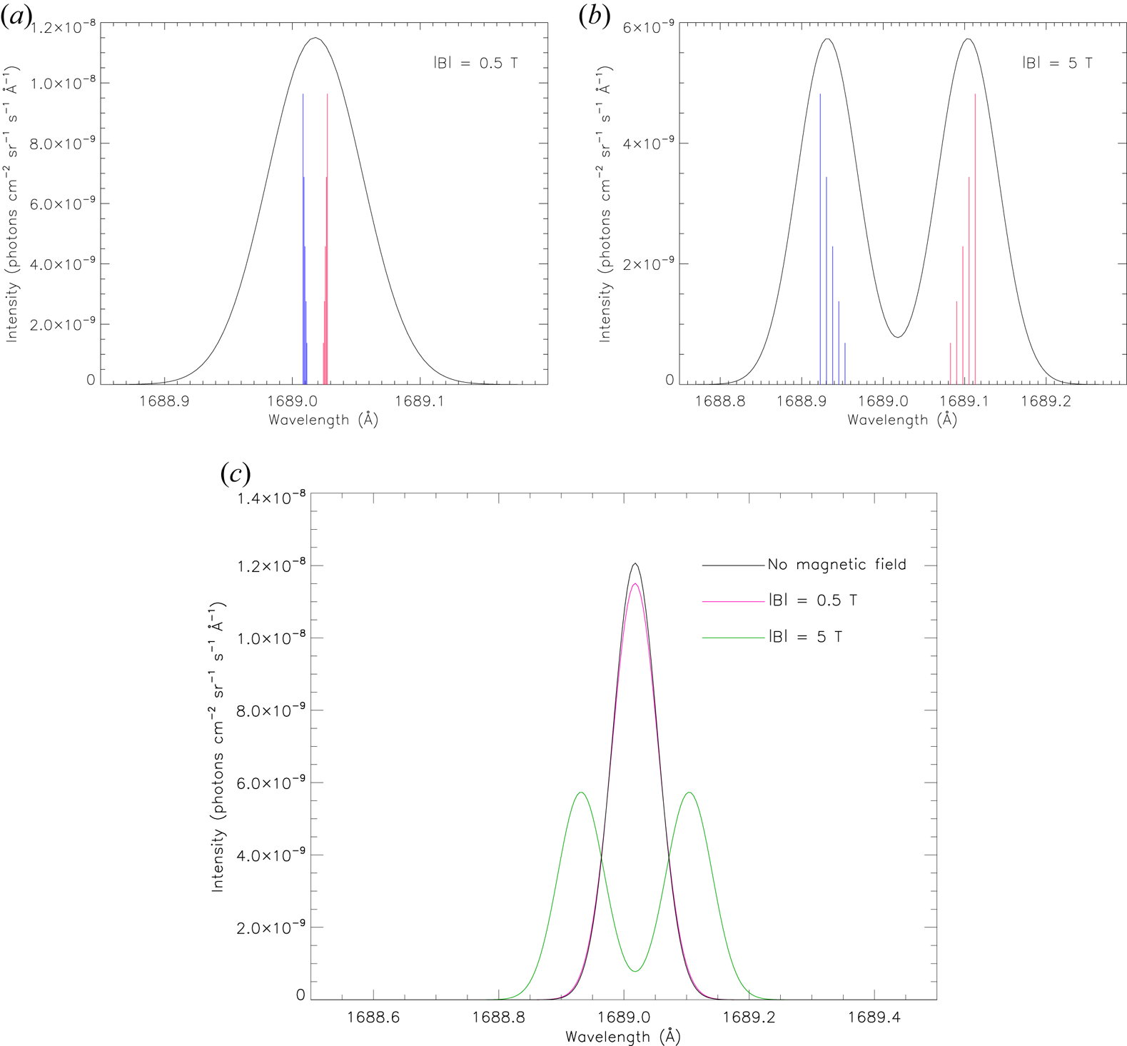
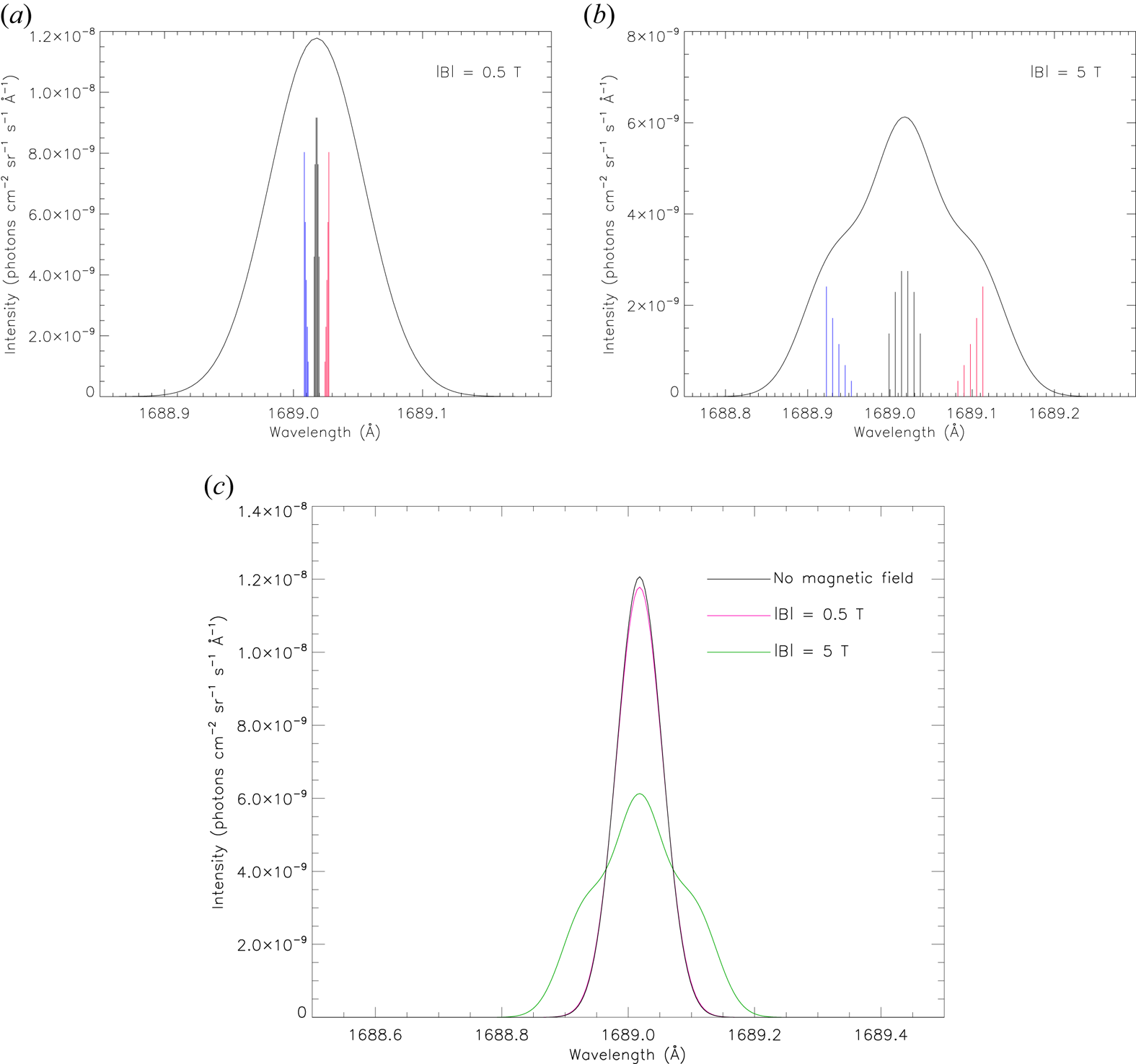
The use of a spectrograph only allows to acquire the line intensities, i.e. Stokes  $I$ profile if the plasma is magnetized which differs in shape from the spectrum of a non-magnetized plasma. In this regard, for the Fe X line in the ultraviolet range we compared the emission expected in absence of
 ${\boldsymbol {B}}$ with the ones in presence of magnetic fields
 $|{\boldsymbol {B}}| = 0.5$ T and
 $5$ T, both observed along the field direction (
 $\theta = 0^{\circ }$,
 $\chi$ undefined) and perpendicularly to the field (
 $\theta = 90^{\circ }$,
 $\chi = 0^{\circ }$). Results are shown in figures 7 and 8, respectively, where profiles are plotted adopting
 $R =20\,000$.
(a,b) Stokes  $I$ profiles of the iron line Fe X 1689.0179 Å as observed along the field direction (
 $\theta = 0^{\circ }$,
 $\chi$ undefined), computed by CHIANTI in presence of a magnetic field (a)
 $|{\boldsymbol {B}}| = 0.5$ T and (b)
 $5$ T. Blue and red marks show the wavelength positions of the blueshifted and redshifted
 $\sigma$ components, respectively. (c) Comparison between the line profiles above and the one expected in absence of magnetic fields.

(a,b) Stokes  $I$ profiles of the iron line Fe X 1689.0179 Å as observed perpendicularly to the magnetic field (
 $\theta = 90^{\circ }$,
 $\chi = 0^{\circ }$), computed by CHIANTI in presence of (a)
 $|{\boldsymbol {B}}| = 0.5$ T and (b)
 $5$ T. Blue and red marks show the wavelength positions of the blueshifted and redshifted
 $\sigma$ components, respectively. (c) Comparison between the line profiles above and the one expected in absence of magnetic fields.

5 Conclusions
Emission spectroscopy will have a fundamental role in characterizing the ion emission of laboratory plasmas. By means of high-resolution échelle spectrographs, covering thousands of Å in a single exposure, plasma spectroscopy is ready to provide measurements of a large number of plasma parameters such as velocity fields, element abundances and thermal properties. In addition, the full Stokes high-resolution spectropolarimetry will make it possible to study the magnetic field structure inside of the laboratory plasma chamber as well as the phenomena of magnetic reconnection and annihilation.
The inclusion of the Zeeman effect in CHIANTI represents the first fundamental step towards a three-dimensional characterization of the magnetic field geometry and element-by-element distribution in laboratory plasmas. To achieve the final result, further very difficult steps are necessary:
(i) integrate the COdice per la Sintesi Spettrale nelle Atmosfere Magnetiche (see Stift, Leone & Cowley (Reference Stift, Leone and Cowley2012), for the last COSSAM version) into CHIANTI to compute the emitted plasma spectrum in the four Stokes parameters in the more realistic case of inhomogeneous plasmas along the line of sight, with varying element abundances, magnetic field strength and direction, and plasma parameters;
(ii) develop inversion techniques to recover the three-dimensional plasma conditions from the observed plasma spectrum (Leone et al. Reference Leone, Scalia, Gangi, Giarrusso, Munari, Scuderi, Trigilio and Stift2017; Stift & Leone Reference Stift and Leone2017a,Reference Stift and Leoneb); and
(iii) enhance the polarization signal across line profiles with coadding techniques (Semel et al. Reference Semel, Ramírez Vélez, Martínez González, Asensio Ramos, Stift, López Ariste and Leone2009; Scalia et al. Reference Scalia, Leone, Gangi, Giarrusso and Stift2017).
Acknowledgements
CHIANTI is a collaborative project involving George Mason University, the University of Michigan (USA), University of Cambridge (UK) and NASA Goddard Space Flight Center (USA). We acknowledge financial contribution from the agreement ASI-INAF n.2018-16-HH.0. We also acknowledge the fifth Nat. Comm. of INFN under the grant MAPS_3D. F.L. was supported by ‘Programma ricerca di ateneo UNICT 2020-22 linea 2’.
Editor William Dorland thanks the referees for their advice in evaluating this article.
Declaration of interests
The authors report no conflict of interest.
Appendix A
The relative strengths of the Zeeman components are expressed through the 3-j symbols (§ 3). These quantities, due to the coupling of angular momenta in two quantum systems, can be computed through the Racah formula (1942); for integer or half-integer values  $a$,
 $b$,
 $c$,
 $\alpha$,
 $\beta$,
 $\gamma$ as follows:
 \begin{equation} \left(\begin{matrix} a & b & c\\ \alpha & \beta & \gamma \end{matrix}\right) = (-1)^{a-b-\gamma} \times \sqrt{\varDelta(a, b, c)} \times F \times \sum_t \frac{(-1)^t}{T}, \end{equation}
with
 \begin{align} \left.\begin{array}{c@{}} \varDelta (a, b, c) = \dfrac{(a+b-c)! (a-b+c)! (-a+b+c)!}{(a+b+c+1)!} \\ F = \sqrt{(a+\alpha)! (a-\alpha)! (b+\beta)! (b-\beta)! (c+\gamma)! (c-\gamma)!} \\ T = t! (c-b+t+\alpha)! (c-a+t-\beta)! (a+b-c-t)! (a-t-\alpha)! (b-t+\beta)! \end{array}\right\}, \end{align}
for all integers  $t$ giving non-negative factorials. The 3-j symbol is not null only if the conditions
 $\alpha + \beta + \gamma = 0$ and
 $|a - b| \le c \le a + b$ are both satisfied.