

1 Introduction
An error-driven learner entertains a current hypothesis of the target grammar and slightly updates this hypothesis whenever it makes an error on the current piece of data. The computational theory of error-driven learning provides guarantees for four core requirements: convergence (is the number of errors made by the learner finite?), efficiency (is the number of errors also small?), stochastic tolerance (does the number of errors remain small for the stochastic implementation?) and noise robustness (does it remain small in the presence of noisy data?).Footnote 1 Within constraint-based phonology, these computational guarantees can be derived using two approaches (Tesar & Smolensky Reference Tesar and Smolensky2000: §1.2): the constraint-independent approach derives computational guarantees from just the formal mode of constraint interaction; the constraint-dependent approach instead resorts to substantive assumptions on the phonological constraints. This paper compares error-driven learning within two frameworks for constraint-based phonology: Harmonic Grammar (HG; Legendre et al. Reference Legendre, Miyata and Smolensky1998a, Reference Legendre, Miyata and Smolenskyb, Smolensky & Legendre Reference Smolensky and Legendre2006) and Optimality Theory (OT; Prince & Smolensky Reference Prince and Smolensky2004). The OT learner is endowed with computational guarantees for efficiency, stochastic tolerance and noise robustness which hold independently of any substantive assumptions on the constraints. This paper shows that the HG learner does not admit such constraint-independent guarantees. Any guarantees of efficiency, stochastic tolerance and noise robustness in HG thus need to be restricted to specific constraint sets.
The paper is organised as follows. §2 outlines the logical structure of the computational theory of error-driven learning in constraint-based phonology. §3 introduces the OT and HG implementations of error-driven learning. §4 compares the two implementations from the perspective of efficiency, and presents a counterexample where the number of errors made by the HG learner grows so fast with the number of constraints that the learner makes over five million errors to assign weights to just ten constraints. Despite the fact that the corresponding HG and OT typologies coincide, the OT learner instead makes fewer than fifty errors, as we would expect, given its constraint-independent efficiency guarantees (Tesar & Smolensky Reference Tesar and Smolensky1998, Magri Reference Magri2012b). §5 extends the comparison to the stochastic implementation of error-driven learning. It shows that the number of additional errors made by the HG stochastic learner, on top of the already astronomical number of errors made by the deterministic learner, grows fast with the number of constraints: the stochastic HG learner run on the counterexample with just ten constraints makes over one million additional errors. The OT stochastic learner makes only around 150 additional errors, as expected because of its constraint-independent guarantees of stochastic tolerance (Magri Reference Magri2016). Finally, §6 extends the comparison to the noisy learning setting. It shows that the number of additional errors made by the HG learner because of noisy training data grows so fast that a single small update by a noisy piece of data (which changes at most three of the ten weights by only a small amount) requires over 60,000 additional updates to recover. The OT learner makes only nine additional errors, as expected from its constraint-independent guarantees of noise robustness (Magri Reference Magri2016). §7 concludes with a discussion of the implications of these results for phonological theory and language acquisition.
This paper contributes to the current debate between the OT and HG implementations of constraint-based phonology (Pater Reference Pater2009) from the perspective of (error-driven) learnability. Even if HG turns out in the end to be better motivated than OT from a typological perspective, the counterexamples discussed in this paper and their detailed analyses are still relevant, as they focus the HG research agenda on the learnability implications of substantive constraint restrictions.
2 The computational theory of error-driven learning in constraint-based phonology
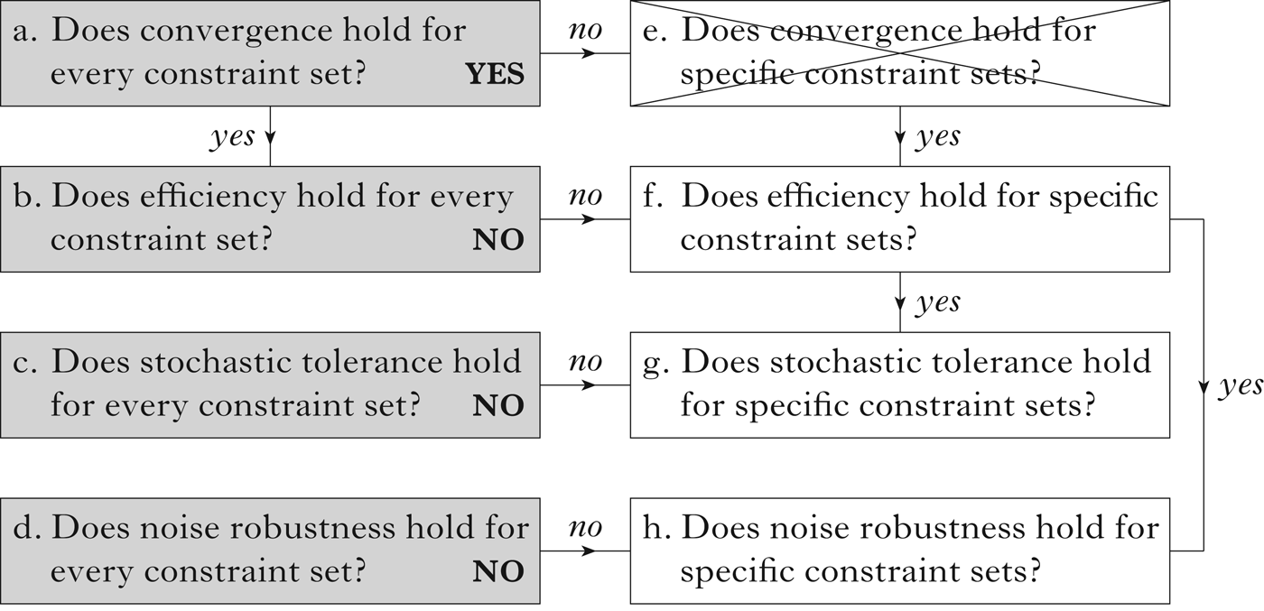
This section outlines the logical structure of the computational theory of error-driven learning in constraint-based phonology, building towards the synopsis in Fig. 4 in §2.5.
2.1 Convergence and efficiency
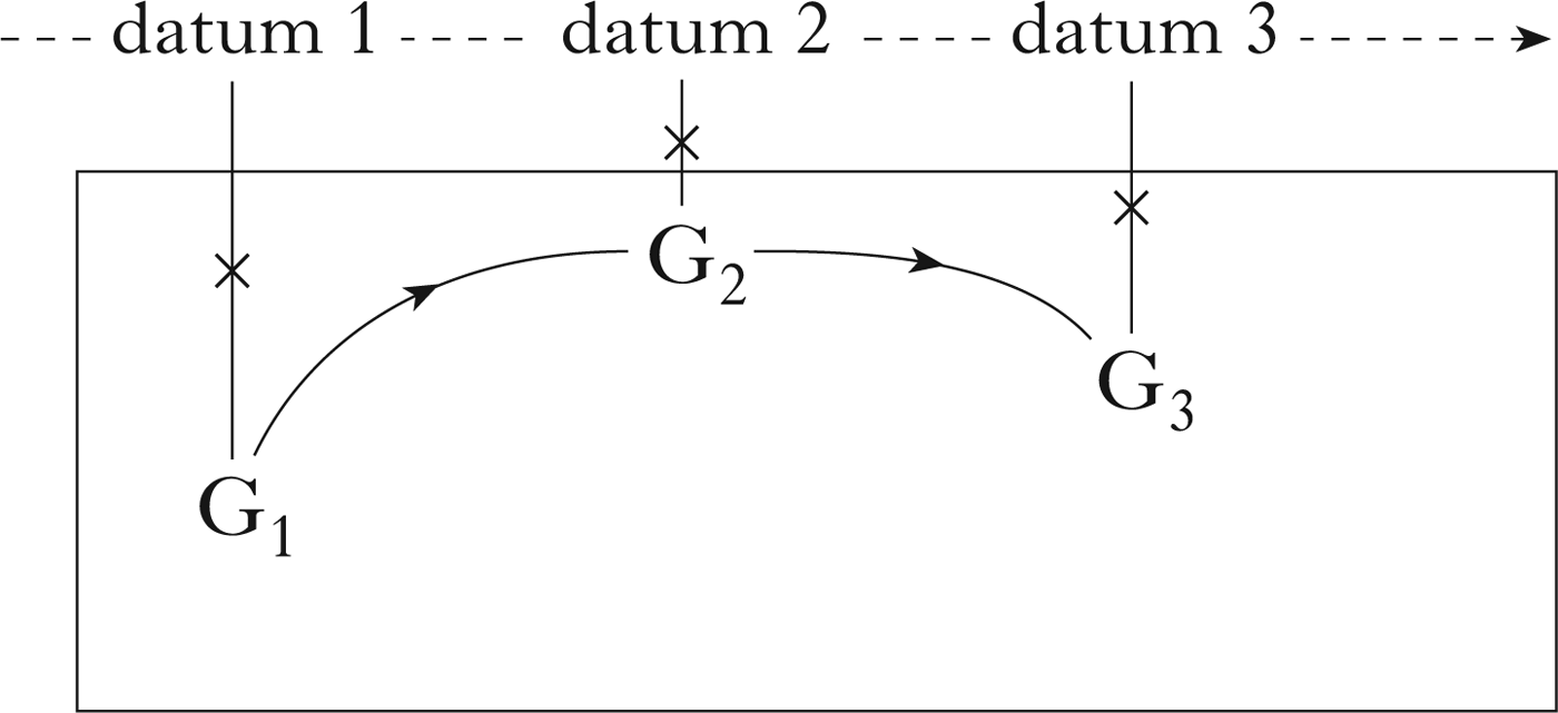
Assume that the learner is provided with the space of grammars G1, G2, etc. The learner maintains a current grammar, which represents its current hypothesis on the target adult grammar. Data come in a stream. Whenever the current grammar (say G1) makes an error on the current piece of data (say datum 1), it is updated to a slightly different one (say G2). The current piece of data is then discarded, and the learner waits for the next piece of data to evaluate the performance of the updated grammar, as in Fig. 1.
Schematic representation of error-driven learning.

This learning scheme is called error-driven because the learning dynamics are driven by the errors made on the incoming stream of data. This scheme has been thoroughly investigated in the machine learning literature (under the heading of online learning; for reviews, see Kivinen Reference Kivinen, Mendelson and Smola2003, Cesa-Bianchi & Lugosi Reference Cesa-Bianchi and Lugosi2006: chs 11, 12 and Mohri et al. Reference Mohri, Rostamizadeh and Talwalkar2012: ch. 7). Within the language-acquisition literature, this learning scheme has been endorsed at least since Wexler & Culicover (Reference Wexler and Culicover1980), for two reasons. First, an error-driven learner describes a sequence of grammars in the typological space which provides a tool to model child acquisition paths. Second, an error-driven learner does not keep track of previously seen data: the current piece of data is compared with the current grammar and then discarded.Footnote 2 It is thus perfectly suited to model the early stages of language acquisition prior to the development of the native language lexicon, such as the early acquisition of phonotactics (Hayes Reference Hayes2004).
The most basic question of the computational theory of error-driven learning concerns convergence: is it possible to guarantee that the learner makes only a finite number of errors? Convergence is crucial, because it entails that the learner eventually settles on a final grammar which will never be further updated and thus counts as the grammar learned by the algorithm. Of course, there is little difference between the number of errors being infinite and it being finite but astronomically large. The next crucial question of the computational theory of error-driven learning thus concerns efficiency: is the number of errors not only finite but also small enough that the final grammar is efficiently converged on? Of course, the number of errors made by the learner should be allowed to grow with the complexity of the learning task. In constraint-based phonology, the simplest measure of complexity is the number of phonological constraints. Thus the number of errors is ‘small’ (and the learner efficient) provided it grows slowly (polynomially) with the number of constraints.
2.2 Stochastic tolerance
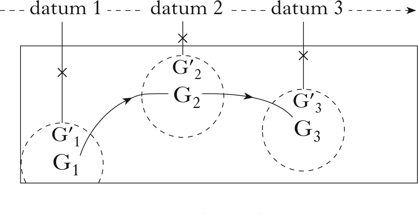
The implementation of error-driven learning schematised in Fig. 1 is called deterministic, to distinguish it from the stochastic implementation (Boersma Reference Boersma1997, Reference Boersma1998, Boersma & Hayes Reference Boersma and Hayes2001, Coetzee & Pater Reference Coetzee and Pater2008, Reference Coetzee, Pater, Goldsmith, Riggle and Yu2011, Coetzee & Kawahara Reference Coetzee and Kawahara2013, Jarosz Reference Jarosz2013, Boersma & Pater Reference Boersma, Pater, McCarthy and Pater2016) schematised in Fig. 2. The latter differs because the current piece of data (say datum 1) is compared not with the current grammar (say G1), but with a variant thereof (say G′1), sampled from the neighbourhood of the current grammar (shown as a circle centred at G1).
Schematic representation of stochastic error-driven learning.

Assume that the stochastic error-driven learner is trained on a sequence of data generated by some (deterministic) target grammar.Footnote 3 In the worst-case scenario, the stochastic learner can make more errors than the deterministic learner, because the stochastic component can derail the learner from the most straightforward learning path (the simulations reported in §5 will show that to indeed be the case). The worst-case number of errors made by a stochastic learner can thus be expressed as the sum of two terms, as in (1). The first is the worst-case number of errors made by the deterministic learner, which measures the difficulty of error-driven learning. The second is the worst-case number of additional errors made by the stochastic learner, which measures the slow-down due to the stochastic implementation.
-
(1)


The next question for the theory of error-driven learning concerns its tolerance of the stochastic component: is the number of additional errors due to the stochastic implementation (the second term on the right-hand side of (1)) small enough not to disrupt efficiency? Again, this number of additional errors should be allowed to grow with the complexity of the learning task, measured as the number of constraints. Thus the number of additional errors is ‘small’ (and the learner tolerant of the stochastic component) provided it grows slowly (polynomially) with the number of constraints.Footnote 4
2.3 Noise robustness
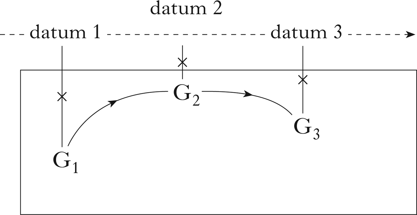
So far, I have assumed that the learner is trained on a stream of pristine data generated by some target grammar in the typology. A more realistic learning setting needs instead to allow for the possibility that a small portion of the training data could have been corrupted by transmission noise or speech errors (Gibson & Wexler Reference Gibson and Wexler1994, Frank & Kapur Reference Frank and Kapur1996, Boersma & Hayes Reference Boersma and Hayes2001, Bíró Reference Bíró2006). I schematise this more realistic noisy setting as in Fig. 3, where the data not located on the dotted line (such as datum 2) are meant to be corrupted by noise and thus inconsistent with the rest of the pristine data.
Schematic representation of error-driven learning in a noisy setting.

Suppose that the (possibly infinite) sequence of pristine training data is interspersed with a finite amount of data corrupted by noise. No assumptions are made on the corrupted data apart from there being only a finite number.Footnote 5 The corrupted data make the learning problem harder (Magri Reference Magri2013a: §2), and might thus force the learner to make more errors. In other words, the number of errors made by the learner on a possibly corrupted training sequence can be expressed as the sum of two terms, as in (2). The first term is the number of errors which would have been made on the sequence of pristine data with the corrupted data removed, and the second is the number of additional errors due to the corrupted data.
-
(2)

The final question for the theory of error-driven learning concerns its robustness to noise: is the number of additional errors due to the corrupted data small enough not to disrupt efficiency? Again, the number of additional errors should be allowed to grow with the complexity of the learning task, measured as the number of constraints (as well as, of course, the number of pieces of corrupted data and the size of the faulty updates they cause). Thus the number is ‘small’ (and the learner robust to noise) provided it grows slowly (polynomially) with the number of constraints.
2.4 Constraint-dependent and independent perspectives
Tesar (Reference Tesar2013: 18) summarises the core tenet of generative linguistics as follows: ‘for language learning to be possible, the linguistic theory must have some kind of non-trivial structure … that can be exploited by a learner’. What type of non-trivial structure yields guarantees for convergence, efficiency, stochastic tolerance and noise robustness of error-driven learning? Within constraint-based phonology, ‘phonological theory contains two parts: a theory of substantive universals of phonological well-formedness and a theory of formal universals of constraint interaction’ (Prince & Smolensky Reference Prince and Smolensky2004: 80). Correspondingly, computational guarantees for error-driven learning can be developed from either of two perspectives (Tesar & Smolensky Reference Tesar and Smolensky2000: §1.2). The constraint-independent perspective derives computational guarantees from the formal properties of the mode of constraint interaction alone (e.g. the logic of transitive orders in the case of OT or the linear algebra underlying HG). It does not make any substantive assumptions on the phonological content of the constraints. The constraint-dependent perspective instead derives computational guarantees from the additional structure brought about through substantive restrictions on the phonological content of the constraints.Footnote 6 It is standard practice in the literature to adopt the constraint-independent perspective as the starting point, and to resort to the alternative constraint-dependent perspective only when the former fails. For instance, Eisner (Reference Eisner, Eisner, Karttunen and Thériault2000: 23) writes: ‘The algorithms for learning … are designed to be general for any [constraint set] … That is, these methods are not tailored (as others might be) to exploit the structure of some specific, putatively universal [constraint set]’. The main reason for the privileged status accorded to the constraint-independent perspective is that, when it succeeds, it yields stronger results, namely computational guarantees that hold for a completely arbitrary constraint set. It thus circumvents the contentious issue of characterising phonologically plausible constraint sets, and it ensures that the computational theory won't have to be revised whenever new phonological data are uncovered or better analyses developed.
2.5 Summary
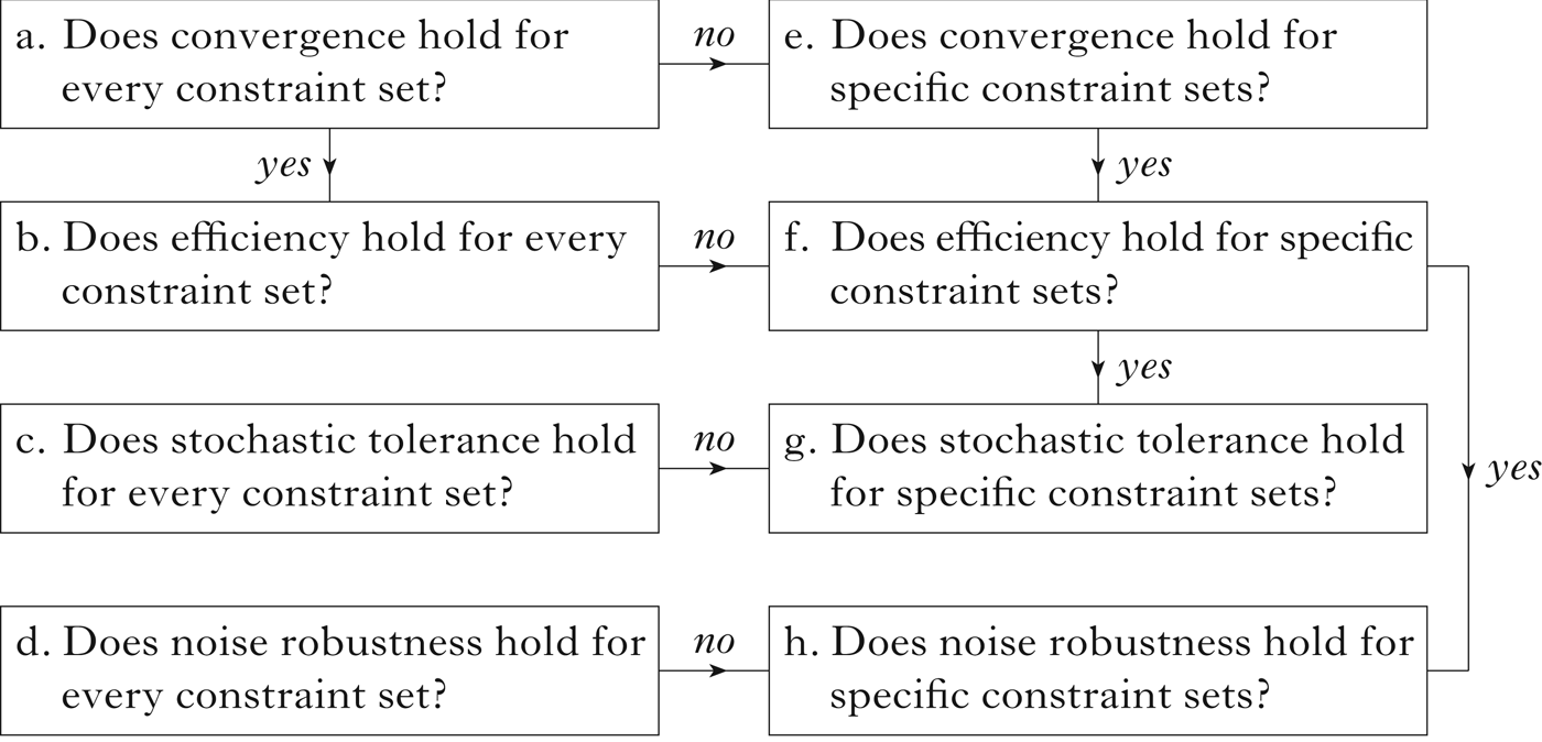
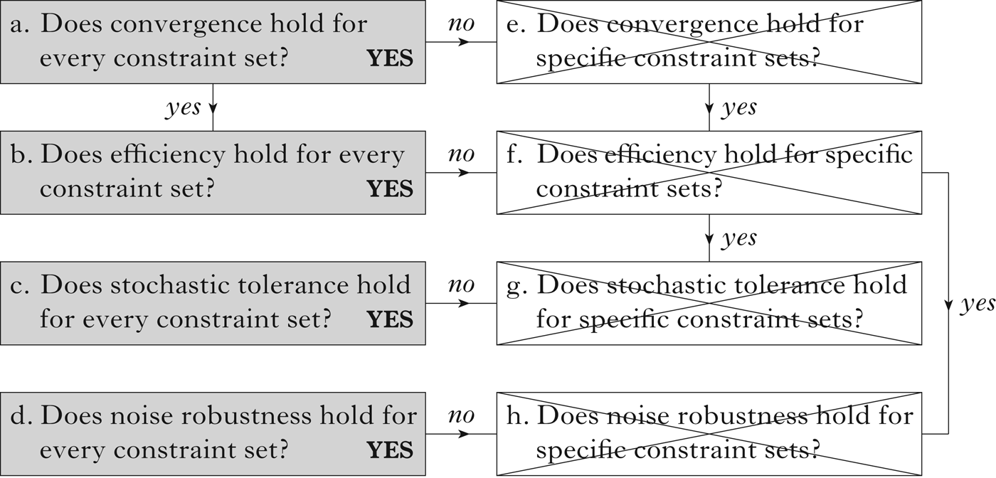
The computational theory of error-driven learning in constraint-based phonology outlined in this section is summarised in Fig. 4. The theory aims at computational guarantees for convergence, efficiency, stochastic tolerance and noise robustness, corresponding to the four rows. It adopts a constraint-independent or dependent perspective, corresponding to the two columns. The horizontal arrows encode the privileged status accorded to the constraint-independent perspective: they say that a constraint-dependent question (in the right column) is tackled only when the corresponding constraint-independent question (in the left column) has been answered negatively. The vertical arrows encode additional dependencies among the eight questions. For instance, it only makes sense to investigate efficiency (i.e. whether the number of errors is small) if convergence has been established (i.e. the number of errors is finite), as encoded by the two arrows between questions (a) and (b) and between (e) and (f). Furthermore, it only makes sense to investigate stochastic tolerance and noise robustness for a certain constraint set after efficiency has been established for that constraint set, as encoded with the two arrows between question (f) and questions (g) and (h). In fact, a learner which is inefficient in its deterministic implementation and in a noise-free setting is useless to start with. On the other hand, even if efficiency fails from the ambitious constraint-independent perspective, it could still be the case that the number of additional errors in (1) and (2) due to the stochastic implementation or the noisy data remains small for any constraint set. There is therefore no arrow relating question (b) to (c) and (d).
Structure of the computational theory of error-driven learning in constraint-based phonology.

3 Error-driven learning in OT and HG
3.1 Algorithmic core
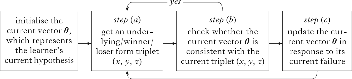
The HG typology of grammars is parameterised with a weight vector θ = (θ 1, θ 2, …), which assigns a weight θ k to each constraint C k . The OT typology is parameterised with a constraint ranking. A ranking can be represented numerically with a ranking vector θ = (θ 1, θ 2, …), which assigns a ranking value θ k to each constraint C k : a constraint is ranked above another constraint whenever the ranking value of the former is larger than the ranking value of the latter (Boersma Reference Boersma1997, Reference Boersma1998, Reference Boersma2009). The error-driven learning scheme sketched in Fig. 1 can then be formalised as in Fig. 5 within either HG and OT. The learner maintains a current vector θ of weights or ranking values. For concreteness, I assume that its components are initially set all equal to zero. The current vector θ is then updated by looping through steps (a)–(c). At step (a), the learner receives the current piece of data. At step (b), it checks whether the OT or HG grammar corresponding to the current vector θ is consistent with that piece of data. If that is the case, the learner has nothing to learn from the current piece of data, loops back to step (a) and waits for more data. Otherwise, the learner updates the current vector θ at step (c) and then loops back to step (a) and starts all over again. The rest of this section describes steps (a)–(c).
Algorithmic core of error-driven learning in HG and OT.

3.2 Data
At step (a) in Fig. 5, the learner receives a piece of data. At a minimum, this piece of data consists of a surface form y, say some form which is licit according to the phonotactics corresponding to the target grammar the learner is being trained on. In some applications, the corresponding underlying form x can be assumed to be provided as well. In other applications, the learner instead needs to be endowed with an additional subroutine to reconstruct the underlying form (e.g. set the current underlying form x identical to the current surface form y; Hayes Reference Hayes2004, Prince & Tesar Reference Prince and Tesar2004, Magri Reference Magriforthcoming). Since this paper abstracts away from the proper definition of this subroutine, the underlying form is assumed to be provided along with the surface form at step (a). The mapping (x, y) of the underlying form x to the surface form y must beat the mapping (x, ƶ) of x to any other loser candidate ƶ (I adopt the convention of striking out loser candidates). The learner thus needs to focus on one such loser candidate. Usually, this loser candidate is chosen through a proper subroutine. This paper also abstracts away from the proper definition of this subroutine. The loser form is thus assumed to be provided along with the underlying and winner forms at step (a). In the end, the piece of data fed to the learner at step (a) consists of an underlying/winner/loser triplet (x, y, ƶ).
3.3 Update conditions
At step (b) in Fig. 5, the error-driven learner checks whether the HG or OT grammar corresponding to the current weight or ranking vector θ = (θ 1, θ 2, …) is consistent with the current underlying/winner/loser form triplet (x, y, ƶ), i.e. whether it makes the current winner y beat the current loser ƶ for the underlying form x. In the case of HG, this consistency condition is (3). The violation difference corresponding to constraint C k is the difference between the number of violations C k (x, ƶ) it assigns to the loser ƶ minus the number of violations C k (x, y) it assigns to the winner y. Condition (3) thus requires the average of the constraint-violation differences weighted by the weights θ k to be strictly positive.
-
(3)

In the case of OT, the consistency condition checked at step (b) is (4). This condition requires the highest-ranking value among the winner-preferring constraints in W (i.e. those constraints which have a positive violation difference, assigning fewer violations to the intended winner than to the intended loser) to be larger than the highest-ranking value among the loser-preferring constraints in L (those constraints which have a negative violation difference, assigning more violations to the intended winner than to the intended loser).Footnote 7
-
(4)

Conditions (3) and (4) will be referred to as the HG and OT update conditions, as the learner performs an update only in case these conditions fail. Note that neither update condition depends on the actual number of constraint violations, but only on the constraint-violation differences.
3.4 Update rules
At step (c) in Fig. 5, the error-driven learner updates the current weight or ranking vector in case the corresponding grammar has failed on the current piece of data. In the case of HG, the literature has adopted the perceptron (or ‘delta’) update rule in (5) (Coetzee & Pater Reference Coetzee and Pater2008, Reference Coetzee, Pater, Goldsmith, Riggle and Yu2011, Jesney & Tessier Reference Jesney and Tessier2011, Coetzee & Kawahara Reference Coetzee and Kawahara2013, Boersma & Pater Reference Boersma, Pater, McCarthy and Pater2016). If a constraint C k is winner-preferring (or loser-preferring), its violation difference C k (x, ƶ) − C k (x, y) is positive (or negative), so that its weight is increased (or decreased) by (5). I refer to the algorithm in Fig. 5 with the HG update condition in (3) at step (b) and the reweighting rule in (5) at step (c) as the (perceptron) HG error-driven learning algorithm.Footnote 8
-
(5)

Despite its wide use in the current HG literature, this perceptron update rule runs into the following problem. Constraints express penalties in constraint-based phonology, never rewards (Keller Reference Keller2000, Legendre et al. Reference Legendre, Sorace and Smolensky2006). Constraint weights must therefore be required to be non-negative in order for HG to avoid undesired typological predictions. Yet the perceptron reweighting rule in (5) does not in any way guarantee non-negativity of the current and final weights entertained by the learner. A natural strategy to overcome this problem is to resort to the variant in (6), which truncates the updates at zero (Boersma & van Leussen Reference Boersma and van Leussen2014: §5, Magri Reference Magri2015, Boersma & Pater Reference Boersma, Pater, McCarthy and Pater2016: 19). The algorithm in Fig. 5 with the HG update condition (3) at step (b) and this new reweighting rule (6) at step (c) can be called the truncated perceptron HG learner.
-
(6)

Turning to OT, the generic reranking rule used by the error-driven learner at step (c) in Fig. 5 is given in (7). The promotion component (7a) of the reranking rule promotes the winner-preferring constraints by a promotion amount which is equal to the inverse of the number w of winner-preferring constraints scaled by a constant c (Magri Reference Magri2012b). This constant, used to calibrate the promotion amount on the number of winner-preferring constraints, can be zero (in which case the learner performs no constraint promotion) or positive. In the rest of the paper, I will assume that c is larger than zero, so that the reranking rule performs both constraint demotion and promotion and thus comes closer to the reweighting rule (5)/(6) used by the HG learner. To illustrate, if c = 1/2 (this is the choice used in the simulations reported in the rest of the paper; see Appendix E) and there are three winner-preferring constraints, each will be promoted by c/w = 1/6.
-
(7)

The demotion component (7b) of the reranking rule demotes by a fixed amount (say 1) those loser-preferring constraints that really need to be demoted, namely those that are not currently ranked underneath a winner-preferring constraint, and are therefore undominated (Tesar & Smolensky Reference Tesar and Smolensky1998). The algorithm in Fig. 5 with the update condition (4) at step (b) and the reranking rule (7) at step (c) is a (calibrated and gradual) OT error-driven ranking algorithm. Note that both the HG reweighting rules and the OT reranking rule do not depend on the actual number of constraint violations, but only on the constraint-violation differences.
3.5 Stochastic implementation
At step (b) in Fig. 5, the deterministic error-driven learner checks the update condition (3) or (4) for HG and OT respectively. The only innovation of the stochastic implementation sketched in Fig. 2 is that the update condition is checked not for the current weights or ranking values θ 1, θ 2, …, but for their stochastic counterpart θ 1+ε 1, θ 2+ε 2, …, where ε 1, ε 2, … are sampled independently from each other. The algorithm in Fig. 5 with this stochastic update condition at step (b) is called the OT/HG stochastic error-driven learner (Boersma Reference Boersma1997, Reference Boersma1998).Footnote 9 The stochastic values εk are usually sampled according to a Gaussian distribution, with zero mean and small variance. Since the tails of the Gaussian distribution decrease exponentially fast, these stochastic values are bounded with high probability between some thresholds −Δ and +Δ. From an analytical perspective, it is nonetheless convenient to assume they are deterministically bounded, i.e. sampled according to a distribution concentrated between −Δ and +Δ. The analyses carry over with high probability to the Gaussian distribution (Magri & Storme Reference Magri and Stormeforthcoming).Footnote 10
4 Convergence and efficiency
This section discusses some counterexamples where the number of errors made by the HG learner grows fast (exponentially) with the number of constraints, showing that efficiency does not hold constraint-independently, contrary to the case of the OT learner.
4.1 A counterexample for the truncated perceptron
Prince & Smolensky (Reference Prince and Smolensky2004: §10.2.2) put forward a simple counterexample to HG error-driven learning.Footnote 11 The counterexample is shown in (8a) for an arbitrary number n of constraints and illustrated in (8b) for n=5.
-
(8)
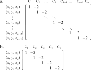
The n constraints C1, C2, …, C n are listed at the top of the matrix in (8). The learner is trained on n−1 underlying/winner/loser form triplets (x, y, ƶ i ), corresponding to a single underlying form x, the winner candidate y, and n−1 loser candidates ƶ 1 , ƶ 2 , …, ƶ n−1. Since the update conditions and update rules described in §3 only depend on the constraint-violation differences, the counterexample is described by providing these violation differences for each constraint and each triplet (for readability, null violation differences are represented with empty entries). Thus the diagonal of entries equal to 1 in (8) shows that constraint C k assigns one more violation to the loser ƶ k than to the winner y. The diagonal of entries equal to −2 shows that constraint C k+1 assigns two more violations to the winner y than to the loser ƶ k . All other violation differences are null.
For concreteness, I focus on the case in (8b), with five constraints. The bottom row of the matrix requires the weight of constraint C4 to be more than twice as large as the weight of C5. The penultimate row requires the weight of C3 to be more than twice as large than the weight of C4 and thus more than 22 = 4 times as large as the weight of C5. And so on until the top row, which requires the weight of C1 to be more than 24 = 16 times as large as the weight of C5. In other words, the weight of C1 starts as null, and has to climb to a final value 2 n−1, which grows exponentially in the number of constraints. Yet the weights are incremented only by 1 with each update, since the positive violation differences in (8) are all equal to 1. We thus expect that a number of updates exponential in n is needed in order to converge to a final weight vector which assigns a sufficiently large weight to constraint C1.
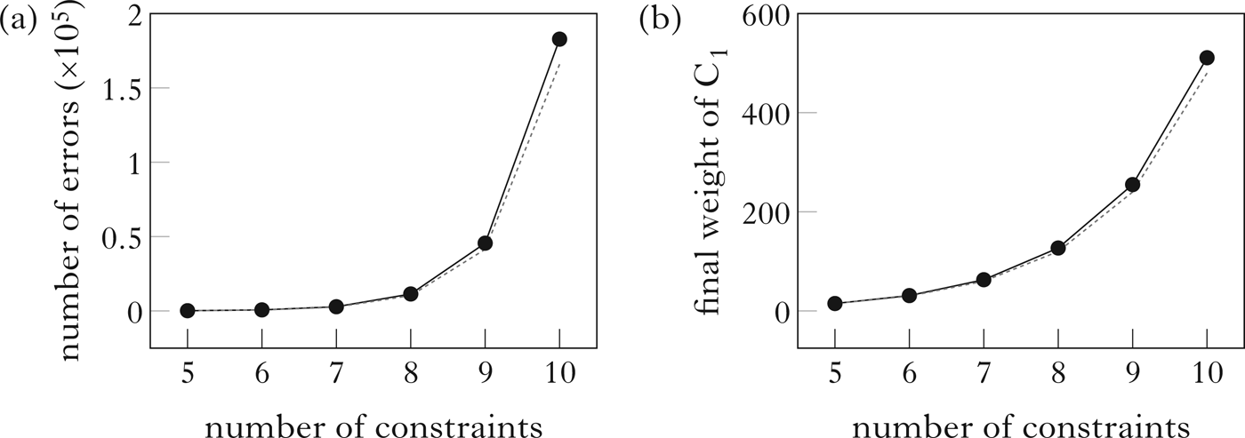
This prediction is borne out in the case of the HG error-driven learner with the truncated perceptron reweighting rule in (6). I ran this learner ten times on the counterexample in (8), with the number n of constraints between five and ten (see Appendix E: Table III for simulation results). The solid line in Fig. 6a plots the largest number of errors made by the HG learner over the ten runs as a function of the number of constraints.Footnote 12 Comparison with the function 162×4 n−5 plotted by the dashed line shows that the number of errors grows fast (exponentially) with the number of constraints.Footnote 13 Indeed, the number of errors grows so fast that the learner makes more than 180,000 errors in the case with ten constraints. The solid line in Fig. 6b plots the final weight of constraint C1 (which is constant across the ten runs) as a function of the number of constraints. Comparison with the function 15×2 n−5 plotted by the dashed line shows that this final weight grows fast (exponentially) with the number of constraints, as predicted by Prince & Smolensky's reasoning. The counterexample in (8) thus shows that no constraint-independent guarantees are possible for the efficiency of the HG error-driven learner with the truncated perceptron reweighting rule. Any such guarantees will have to be restricted through specific assumptions on the constraint set.
Simulation results for the truncated perceptron on counterexample (8).

Yet this counterexample does not defeat the HG learner with the original perceptron reweighting rule in (5). Indeed, that learner converges after only n−1 updates; thus nine updates suffice in the case with ten constraints (see Appendix E: Table V for simulation results). The final weights do not depend on the number of constraints, and are small: the final weight of constraint C1 is always equal to 1, the final weight of constraint C n is always equal to −2, and the other final weights are all equal to −1. By resorting to negative weights, the original perceptron thus defies Prince & Smolensky's challenge. How should we interpret the original and truncated perceptrons’ drastically different performances on the counterexample in (8)? Does it show that the two learners have substantially different properties and that HG's assumption of non-negative weights is particularly troublesome from a learnability perspective? Or is it possible to twist the counterexample to extend it to the original perceptron reweighting rule, thus showing that the two implementations are on a par? The latter turns out to be the case.
4.2 A counterexample to both the original and the truncated perceptron
Consider the counterexample described in (9a) for an arbitrary number of constraints and illustrated in (9b) for the case with five constraints. There are two differences in comparison with the counterexample considered in §4.1 (see §4.3.4 and §4.3.5 for discussion). The first difference is that each negative entry is followed by two positive entries equal to 1, except for the penultimate row (where we can fit only one positive entry after the negative entry) and the last row (where we can fit none). Thus all rows have three positive entries, apart from the penultimate row (which has only two positive entries) and the last row (which has only one). The second difference is that the size of the negative entries is readjusted, so that it is equal to the number of positive entries per row. Thus the negative entry of each row is −3, apart from the penultimate row (whose negative entry is −2) and the last row (whose negative entry is −1).
-
(9)
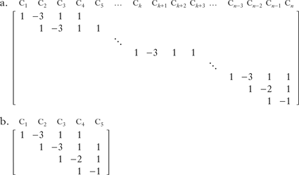
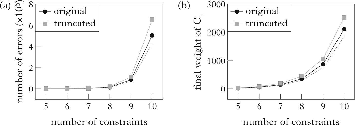
The solid lines in Fig. 7a plot the largest number of errors made by the HG error-driven learner with the two reweighting rules (5) and (6) over ten runs on the counterexample in (9) corresponding to a number of constraints between five and ten (see Appendix E: Tables VI, VII for simulation results). Comparison with the function 550 × 6 n−5 plotted by the dashed line shows that the number of errors grows fast (exponentially) with the number of constraints for both reweighting rules. Indeed, the HG learner with the original perception reweighting rule makes over five million errors in the case with just ten constraints, and over six million with the truncated rule. The solid line in Fig. 7b plots the final weight of constraint C1 in the longest of the ten runs as a function of the number of constraints. Comparison with the function 19 × 2.5 n−5 plotted by the dashed line shows that this final weight again grows fast (exponentially) with the number of constraints.
Simulation results for the original and truncated perceptron on counterexample (9).

I conclude that the counterexample in (9) shows that no constraint-independent efficiency guarantees are possible in the case of the HG error-driven learner, independently of the issue of non-negative weights and thus of the choice between the original and the truncated perceptron reweighting rule. Any efficiency guarantees will have to be restricted through specific assumptions on the constraint set. §4.3 discusses the counterexample in (9).
4.3 Discussion
4.3.1 The margin
The HG error-driven learner with the perceptron reweighting rule (5) converges (Boersma & Pater Reference Boersma, Pater, McCarthy and Pater2016, building on guarantees for the perceptron algorithm: Rosenblatt Reference Rosenblatt1958, Reference Rosenblatt1962, Block Reference Block1962, Novikoff Reference Novikoff1962, Minsky & Papert Reference Minsky and Papert1969, Cristianini & Shawe-Taylor Reference Cristianini and Shawe-Taylor2000: Theorem 2.3, Cesa-Bianchi & Lugosi Reference Cesa-Bianchi and Lugosi2006: ch. 12, Mohri et al. Reference Mohri, Rostamizadeh and Talwalkar2012: ch. 7). Whenever this HG learner is trained on data consistent with some HG grammar and with bounded violation differences, it can only make a finite number of errors, which can be bounded as in (10), in terms of the number of constraints and a quantity that captures a property of the training data, namely their margin (of separability).Footnote 14
-
(10)

The precise definition of the margin (of separability) which appears in the denominator of the error-bound is somewhat involved, and therefore relegated to Appendix A. The following intuitive illustration suffices for the rest of the paper. The error-bound holds under the assumption that the training data are consistent with some HG grammar. Yet consistent training data can differ in their degree of consistency. The data have a high degree of consistency if they are consistent with a certain HG grammar, and remain consistent when the corresponding weight vector is tampered with. The data have a low degree of consistency if even a slight modification of any consistent weight vector affects consistency. The margin which appears in the denominator of (10) can be interpreted as the degree of consistency of the training data. Intuitively, training data with a large degree of consistency should require fewer updates: it should be easier to find a consistent weight vector. While training data with a small degree of consistency should require more updates: a careful aim is required to target a consistent weight vector precisely. The error-bound in (10) formalises this intuition: training data with a high degree of consistency have a large margin, yielding a small error-bound in (10), which provides guarantees for a better performance by the HG learner, and vice versa for training data with a low degree of consistency.
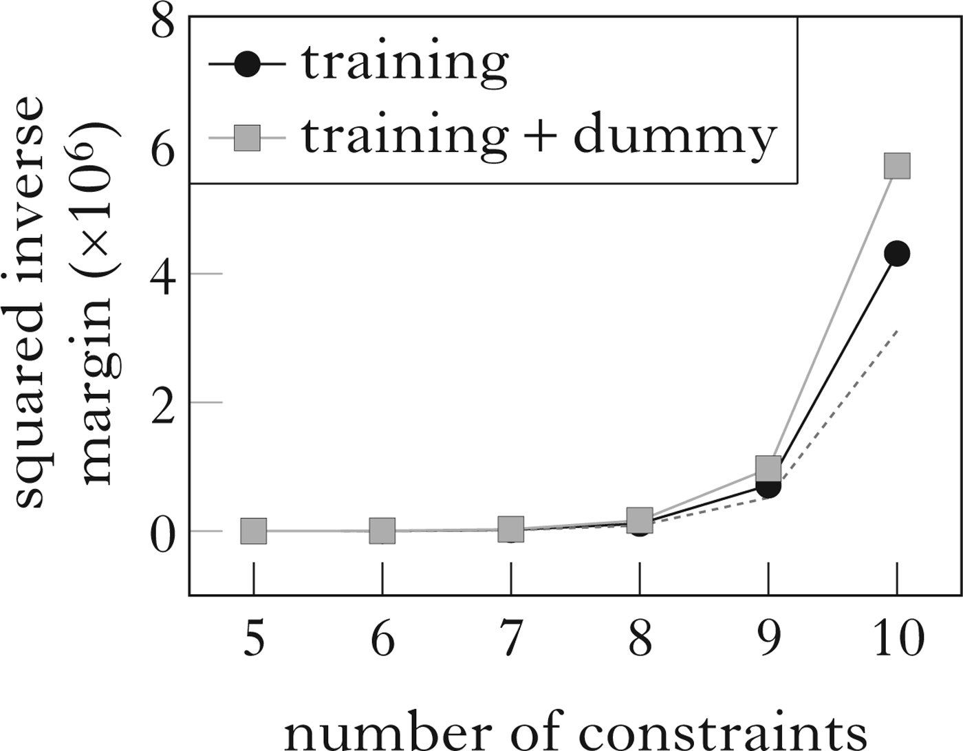
As the number of constraints grows, the constraint interactions can become more subtle and delicate, and the freedom in the choice of the weights thus decreases, shrinking the degree of consistency of the data, namely their margin. If the margin in the denominator of (10) shrinks fast (exponentially) with the number of constraints, it trumps the slow (linear) growth of the numerator. The overall error-bound thus grows fast (exponentially) and provides no guarantees on the efficiency of the HG learner. This is precisely what happens in the case of counterexample (9) – analogous considerations hold for the original counterexample in (8). The inverse of the squared margin is plotted by the black circles in Fig. 8, as computed in Appendix B. Comparison with the function 400×6 n−5 plotted by the dashed line shows that it grows fast (exponentially) with the number of constraints.
Squared inverse margin of separation of the data corresponding to counterexample (9).

In conclusion, the error-bound in (10) settles question (a) in Fig. 4, concerning constraint-independent convergence of the HG perceptron learner. But because of its dependence on the margin, that bound does not settle question (b), concerning constraint-independent efficiency. That question is answered negatively by counterexamples such as the one in §4.2, which shows that constraint-independent efficiency guarantees are impossible.
These considerations extend from the original to the truncated perceptron reweighting rule in (6). To illustrate the intuition, suppose that at a certain iteration the original perceptron demotes the weight of some constraint C k from 0 to the forbidden negative value −1. The truncated perceptron is unable to mimic that demotion and will thus leave the weight of C k at 0. Yet the learning dynamics of the two algorithms can be realigned by assuming that, immediately after that offending demotion, the original perceptron is fed with a piece of dummy data whose constraint-violation differences are all null, apart from the one corresponding to C k , which is +1. Since the current weight of C k is negative, the original perceptron will perform an update in response to this piece of dummy data. This update promotes the weight of C k back to the value 0, where the truncated perceptron had left it. A formalisation of this reasoning (Magri Reference Magri2015) shows that the error-bound in (10) for the original perceptron extends to the truncated variant, only with the margin of the training data replaced by the margin of the training + dummy data, as in (11).
-
(11)

The inverse of the squared margin of the training + dummy data in the case of counterexample (9) is plotted by the grey squares in Fig. 8. Again, it grows fast (exponentially) in the number of constraints, so that the error-bound in (11) for the truncated perceptron HG learner only guarantees constraint-independent convergence, not efficiency.
Extending the training data with additional data can only decrease the degree of consistency, namely the margin. Thus, the margin of the training data extended with the dummy data which appears in the error-bound in (11) for the truncated perceptron should be equal to or smaller than the margin of just the original data which appears in the error-bound in (10) for the original perceptron. The gap between the two solid lines in Fig. 8 quantifies the difference between the two margins in this case. Thus, the error-bound in (11) for the truncated perceptron is worse than (i.e. at least as large as) the error-bound in (10) for the original perceptron. Indeed, the truncated perceptron performs more errors in the simulations plotted in Fig. 7a. The difference between the two margins quantifies the price that needs to be paid for HG's assumption of non-negative weights.
4.3.2 Comparison with OT
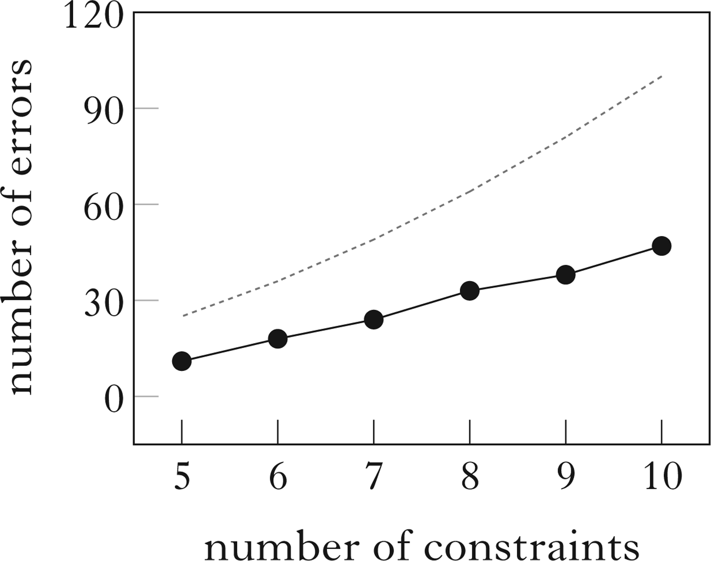
The solid line in Fig. 9 plots the largest number of errors made by the OT learner over ten runs on counterexample (9) corresponding to a number of constraints between five and ten (see Appendix E for simulation details, in particular Table VIII for results). Comparison with the function n2 plotted by the dashed line shows that the number of errors grows slowly (subquadratically) with the number of constraints, so that the learner makes fewer than fifty errors in the case with ten constraints.Footnote 15
Simulation results for the OT learner on counterexample (9).

These simulation results are not surprising. In fact, suppose that the OT learner does not promote ‘too much’, i.e. it adopts a promotion component (7a) corresponding to a calibration constant c which is not ‘too large’, i.e. strictly smaller than 1. Whenever trained on data consistent with some OT grammar, this OT learner converges, and the number of errors is bounded by (12), in terms of the number of constraints and the calibration constant c used in the definition of the promotion amount (Boersma Reference Boersma1997: 323–327, Reference Boersma2009, Tesar & Smolensky Reference Tesar and Smolensky1998, Magri Reference Magri2012a, b).
-
(12)

This error-bound depends on the number of constraints only through its numerator. Thus it grows slowly (quadratically) in the number of constraints. Furthermore, this error-bound requires no assumptions on the constraints. In conclusion, this error-bound provides a positive answer to questions (a) and (b) in Fig. 4 concerning constraint-independent efficient convergence of the deterministic OT error-driven learner.
4.3.3 The OT and HG typologies coincide
The typology of grammars predicted by HG can be larger than the one predicted by OT, because only HG allows gang-up effects.Footnote 16 Could the slowness of the HG learner on the counterexample in (9) relative to the OT learner be due to the fact that the former is exploring a larger typology of grammars? The answer is negative: the counterexample has been constructed in such a way that the HG and OT typologies exactly coincide. To illustrate, consider the case with n=5 constraints in (9b). This matrix of constraint-violation differences corresponds, for instance, to the constraint-violation profiles in (13). For example, the leftmost entry in the top row of matrix (9b) is 1 because (13) says that constraint C1 assigns one violation to the loser ƶ 1 and none to the winner y.
-
(13)
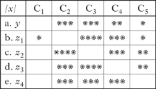
The OT and HG typologies of grammars (computed with OT-Help; Staubs et al. Reference Staubs, Becker, Potts, Pratt, McCarthy and Pater2010) corresponding to the constraint set described in (13) coincide: they both consist of five grammars, one for each mapping of the underlying form to one of the five candidates. This conclusion extends from the case with n=5 constraints to the case with an arbitrary number of constraints: the constraint-violation differences described in (9a) correspond to a set of n constraints whose corresponding OT and HG typologies coincide. The inefficiency of the HG learner on the counterexample thus cannot be due to the fact that it is exploring a larger typology. In other words, the counterexample shows that, even in those cases where the typologies predicted by OT and HG turn out to be identical (as argued to be often the case in Pater Reference Pater2009), the OT parameterisation of the typology outperforms the HG one from the perspective of error-driven learning.
4.3.4 The two crucial properties of the counterexample
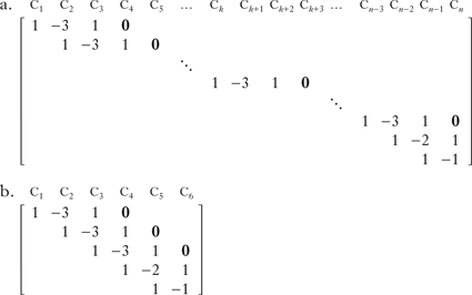
The counterexample in (9) has two properties which are both crucial in order to slow down the HG learner. The first property is that the size of each negative entry is equal to the number of positive entries in the corresponding row (for instance, the negative entry of the penultimate row is −2, because that row has two positive entries). The second property is that each negative entry is followed by two positive entries equal to 1 (except for the last two rows, where there is not enough space to fit in these two extra positive entries). To see that the first property is indeed crucial, consider the variant in (14), where the negative entries are −3 throughout, rather than being −2 and −1 in the bottom two rows. There is no slow-down in this case: with ten constraints, the HG perceptron learner makes only 206 errors, as opposed to the five million errors made on the original counterexample in (9) (see Appendix E: Table IX for simulation results).
-
(14)
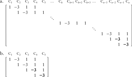
To see that the second property of counterexample (9) is crucial as well, consider the variant in (15), where each negative entry is followed by just one positive entry. Again, there is no slow-down in this case: with ten constraints, the perceptron HG error-driven learner makes only 133 errors, again many fewer than the five million errors made on the original counterexample (see Appendix E: Table X for simulation results).
-
(15)
Why are these two properties crucial in order to defeat the HG learner? The next subsection provides some intuition.
4.3.5 Explaining the two crucial properties of the counterexample
As just noted, one crucial property of counterexample (9) is that the size of the negative entries is always equal to the number of positive entries in the corresponding row. This property ensures that gang-up effects are impossible, as explained in Appendix C (this is a special case of an argument from Magri Reference Magri2013b: §4). The OT and HG update conditions thus collapse: whenever the OT learner would update the current vector θ, the HG learner would update it as well. Furthermore, suppose that the OT learner uses a promotion amount corresponding to c=1 for the calibration constant in (7a). Because of this choice, it turns out that any update made by the OT learner coincides with the update made by the HG learner with the original perceptron reweighting rule, as explained in Appendix C.Footnote 17 We thus reach the following conclusion: since the size of the negative entries in the counterexample is always equal to the number of positive entries, the HG learner with the original perceptron reweighting rule mimics the OT learner with the calibration constant c set to 1. This means that, whenever the OT learner trained on the counterexample makes an update, the HG learner trained on the same sequence of data makes an update as well, and, furthermore, the OT and HG updates exactly coincide. In order for this conclusion to hold, the size of the negative entries needs to be exactly equal to the number of positive entries. For instance, the HG learner does not mimic the OT learner on the variant in (14), where the size of the negative entries in the last two rows is different from the number of positive entries (see Appendix C for a counterexample).
Since the HG learner trained on the counterexample in (9) mimics the OT learner with the value 1 for the calibration constant c, we are prompted to look into the behaviour of this specific OT learner. Magri (Reference Magri2012b: §7.5) reports that the number of errors made by this specific OT learner on the counterexample grows fast (exponentially) in the number of constraints. This fact is not surprising. Since Tesar & Smolensky (Reference Tesar and Smolensky1998: §2.4), there has been a consensus in the OT learnability literature that constraint demotion works well, while constraint promotion is dangerous. The promotion amount (or, equivalently, the calibration constant used to define it) should thus be null, or at least small. It turns out that it is sufficient and necessary for c to be strictly smaller than 1 in order for efficient convergence to hold, as guaranteed by the error-bound in (12). Indeed, even c=1 (the smallest forbidden value) might cause the OT learner to make too many errors, as shown by the counterexample in (9).
The failure of the OT learner when c is equal to the forbidden value 1 on counterexample (9) is due to the second property of the counterexample identified in §4.3.4, namely the fact that each negative entry is followed by two positive entries (except for the last two rows). In fact, the OT learner converges quickly on (15) with fewer additional positive entries, even with the calibration constant c set to the forbidden value 1 (see Magri Reference Magri2013b: §4.8). It is not hard to grasp the intuitive reason why the OT learner is defeated by the two additional positive entries at the right of each negative entry. In fact, each of these entries makes the corresponding constraint winner-preferring. Yet these additional winner-preferring constraints contribute nothing to consistency: counterexample (9) is only consistent with the ranking C1 ⪢ C2 ⪢ … ⪢ C n , just like the variant in (15), with fewer winner-preferring constraints. These additional winner-preferring constraints are thus only a distraction for an OT learner which is too sensitive to them, because it performs too much constraint promotion, i.e. adopts too large a calibration constant. The two layers of additional useless winner-preferring constraints of counterexample (9) suffice to distract the OT learner enough to compromise its efficiency.
In summary, counterexample (9) has two crucial properties, concerning the size of the negative entries (which is equal to the number of positive entries) and the distribution of the positive entries (there are two after each negative entry). The former property of the counterexample ensures that the perceptron HG learner mimics the OT learner with a calibration constant c which is too large, because it is equal to the forbidden value 1. The latter property ensures enough useless winner-preferring constraints to defeat an OT learner which is too sensitive to them, because it sets the calibration constant to 1, and thus promotes too much. In conclusion, the HG learner performs too many updates on (9) because it performs an update whenever the OT learner performs an update; and the latter performs too many updates because it promotes too much. In other words, HG error-driven learning is as bad an idea from a constraint-independent perspective as OT error-driven learning with a large promotion component.
4.3.6 The HG learner is slow even on the most favourable training sequence
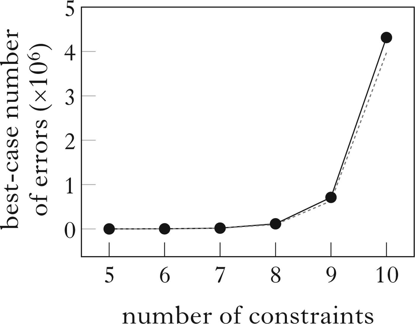
The solid lines in Fig. 7 plot the largest number of errors made by the HG learner over ten runs on the counterexample (9). These simulation results leave open the possibility that there exist some particularly favourable sequences of training data where the learner manages to converge after a smaller number of errors. Such a scenario would leave open the possibility of constraint-independent efficiency guarantees, through proper restrictive assumptions on the training sequences. However, this possibility can be ruled out as well. Appendix D shows how to compute analytically a lower bound on the best-case number of errors made by the HG perceptron learner: it guarantees that the number of errors needed to reach convergence can never be smaller than a certain quantity, even on the most favourable training sequence.Footnote 18 This lower bound on the best-case number of errors is plotted by the solid line in Fig. 10 as a function of the number of constraints between five and ten. Comparison with the function 400 × 6.3 n−5 plotted by the dashed line shows that also the best-case number of errors on the counterexample grows fast (exponentially) with the number of constraints. Furthermore, comparison with the actual number of errors plotted in Fig. 7 shows that the very large number of actual errors in the simulations is very close to the best-case number of errors, and thus cannot be due to particularly unfavourable learning sequences.
Best-case number of errors of the original perceptron on counterexample (9).

4.3.7 The perceptron in machine learning and computational linguistics
How do the counterexamples presented in this section square with the good performance of the perceptron reported in the machine learning and computational linguistics literature? For instance, to advocate the use of the perceptron in HG, Boersma & Pater (Reference Boersma, Pater, McCarthy and Pater2016) mention its successful application in computational linguistics (Collins Reference Collins, Haji and Matsumoto2002). Furthermore, Mohri et al. (Reference Mohri, Rostamizadeh and Talwalkar2012: 168) state that ‘the kernel Perceptron algorithm … [is] commonly used … in a variety of applications’ in machine learning.
There is no contradiction between the counterexamples presented in this section and the results reported in the machine learning and computational linguistics literature on the perceptron. In fact, the latter literature has looked at a variant of the perceptron called the kernel (dual) perceptron. This is the variant mentioned in the preceding quote from Mohri et al. (Reference Mohri, Rostamizadeh and Talwalkar2012) and tested in Collins (Reference Collins, Haji and Matsumoto2002). This variant outperforms the primal perceptron considered here at the expense of a much richer representation of the learning history. In fact, the primal perceptron maintains an impoverished summary of its past learning history: it does not keep track of the previous updates nor of the training data that triggered those updates. The kernel dual perceptron instead stores the (finite) set of training data and maintains a counter (called a dual variable) of the number of updates triggered by each piece of data up to the current iteration. Because of this richer representation of the learning history, the dual perceptron does not fit into the error-driven learning scheme investigated in this paper (see note 2). The conclusions reached in the machine learning and computational linguistics literature concerning the kernel dual perceptron are therefore irrelevant to the topic of this paper, namely the development of proper error-driven learners.
4.4 Summary
This section has compared the OT and HG implementations of error-driven learning from the perspective of constraint-independent efficiency: how fast does the worst-case number of errors grow with the number of constraints? The error-bound for the OT implementation grows slowly with the number of constraints and thus provides constraint-independent efficiency guarantees. The error-bound for the HG implementation instead depends on the margin, and can therefore grow fast with the number of constraints. It is indeed possible to construct cases where the HG and OT typologies coincide, and yet the HG learner makes over five million errors with just ten constraints, which compares poorly with the fewer than fifty errors made by the OT learner. These simulation results show that no constraint-independent efficiency guarantees are possible for the HG learner.
5 Stochastic tolerance
This section discusses some counterexamples where the number of additional errors made by the HG learner because of the stochastic component grows fast (exponentially) with the number of constraints, showing that the learner does not tolerate the stochastic implementation constraint-independently, contrary to the case of the OT learner.
5.1 A counterexample for the original and truncated perceptron
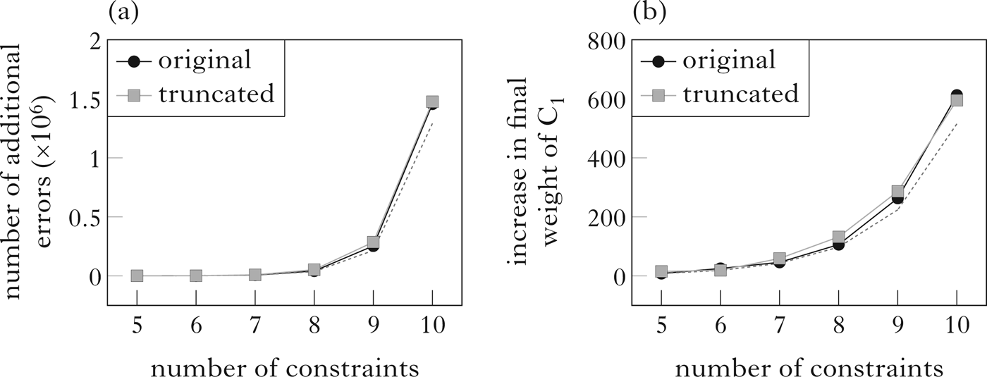
Consider again the counterexample in (9). For each value of the number of constraints between five and ten, I ran the deterministic and stochastic HG learner ten times, with both the original and the truncated perceptron reweighting rule (see Appendix E for simulation details and in particular Tables VI and VII for results). The two solid lines in Fig. 11a plot the difference between the largest number of errors made by the stochastic learner with the two reweighting rules over the ten runs minus the number of errors made by the deterministic learner on that same training sequence. In other words, they plot the additional number of errors due to the stochastic component. Comparison with the function 166×6 n−5 plotted by the dashed line shows that the number of additional errors grows fast (exponentially) with the number of constraints. Indeed, in the case with just ten constraints, the stochastic learner performs almost one and a half million additional errors compared with the deterministic learner, which in turn is already performing over five million errors. For completeness, the solid lines in Fig. 11b plot the difference between the final weight of constraint C1 entertained by the stochastic learner with the two reweighting rules at the end of the longest run minus the final weight of C1 entertained by the deterministic learner at the end of that same run. In other words, they plot the increase in the final weight of constraint C1 due to the stochastic component. Comparison with the function 8 × 2.3 n−5 plotted by the dashed line shows that the increase grows fast (exponentially) with the number of constraints.
Simulation results for the stochastic original and truncated perceptron on counterexample (9).

In conclusion, this counterexample shows that it is not possible to develop constraint-independent guarantees that the HG error-driven learner (with either reweighting rule) tolerates the stochastic implementation, namely that the number of additional errors due to the stochastic component remains small. Any such guarantees will crucially have to be restricted by specific assumptions on the constraint set.
5.2 Discussion
5.2.1 The margin, again
The HG error-driven learner with the stochastic update condition and the original perceptron reweighting rule in (3) provably converges (Boersma & Pater Reference Boersma, Pater, McCarthy and Pater2016). Whenever trained on data consistent with some (deterministic) HG grammar and with bounded constraint differences, it can only make a finite number of errors, which can be bounded as in (16), in terms of the number of constraints and the margin of the training data.Footnote 19 The same error-bound holds for the truncated perceptron reweighting rule in (6), only with the margin of the training + the dummy data (rather than the margin of only the training data) at the denominator (Magri Reference Magri2015).
-
(16)

This error-bound is the sum of two terms. The first term coincides with the error-bound in (10) for the deterministic HG learner. The second term thus quantifies the additional number of errors due to the stochastic implementation, and consists of the number of constraints (scaled by the size Δ of the stochastic component) divided by the squared margin. This term is large (i.e. provides a weak bound) when the margin is small. This makes intuitive sense, given that the margin represents the degree of consistency of the data: a small margin means that there is little freedom in the choice of consistent weights, so that the perturbation of the current weights due to the stochastic component can hold sway. The margin of the counterexample in (9) decreases fast (exponentially) with the number of constraints, so that its squared inverse grows quickly, as plotted in Fig. 8. The bound in (16) on the number of additional errors provided by the second term in (16) thus grows fast, and does not settle question (c) in Fig. 4 concerning constraint-independent stochastic tolerance. That question is answered negatively by the counterexample described in §5.1, which shows that constraint-independent guarantees of stochastic tolerance are impossible in HG.
5.2.2 Comparison with OT
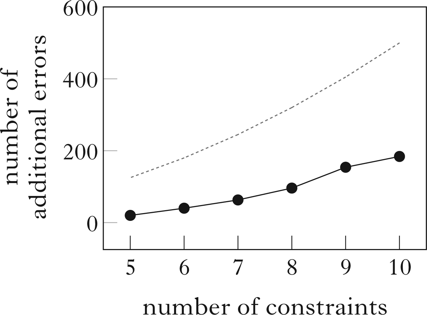
The solid line in Fig. 12 plots the difference between the largest number of errors made by the stochastic OT learner over ten runs on counterexample (9) minus the number of errors made in that same run by the deterministic learner (see Appendix E: Table VIII for simulation results). Comparison with the function 5×n 2 plotted by the dashed line shows that the number of additional errors due to the stochastic component grows slowly with the number of constraints, so that the learner makes fewer than 200 additional errors in the case with ten constraints.Footnote 20
Simulation results for the stochastic OT learner on counterexample (9).

These simulation results are not surprising. In fact, assume that the stochastic OT learner does not promote ‘too much’, i.e. adopts a promotion component (7a) corresponding to a calibration constant which is not ‘too large’ (strictly smaller than 1). Whenever it is trained on data consistent with an OT grammar, the number of errors is bounded by (17), which depends on the number of constraints and on the calibration constant c (Magri Reference Magri2016).Footnote 21
-
(17)

This error-bound in (17) is the sum of two terms. The first term coincides with the error-bound in (12) for the deterministic implementation. The second term thus expresses the number of additional errors due to the stochastic implementation. This additional term grows slowly (quadratically) with the number of constraints. Furthermore, the bound requires no assumptions on the constraints. It thus settles question (c) in Fig. 4 concerning constraint-independent guarantees that the OT learner tolerates the stochastic component.
5.3 Summary
§4 compared the OT and HG deterministic implementations of error-driven learning. This section has extended the comparison to the stochastic implementations. It has focused on the number of additional errors made by the learner because of the stochastic component. The error-bound for the OT stochastic learner provides constraint-independent guarantees that it tolerates the stochastic component. The constraint-independent bound currently available for the HG stochastic learner instead does not guarantee stochastic tolerance, because of its dependence on the margin of the data. Indeed, the HG learner does not tolerate the stochastic implementation constraint-independently: with just ten constraints, the stochastic HG learner can make almost one and a half million additional errors.
6 Noise robustness
This section discusses some counterexamples where the number of additional errors made by the HG learner in response to a small faulty update triggered by a single noisy piece of data grows fast (exponentially) with the number of constraints, showing that noise robustness does not hold constraint-independently, contrary to the OT learner.
6.1 A counterexample for the original and truncated perceptron
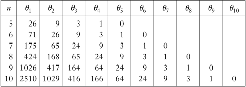
Faulty updates triggered by corrupted data disrupt the current weights or ranking values and thus require additional updates by pristine data to recover. The learner is robust to noise provided the number of updates it takes to recover is small. To estimate noise robustness, we need to inflict the largest damage with each single corrupted piece of data. For concreteness, I focus on the HG learner with the truncated reweighting rule (the reasoning extends straightforwardly to the original perceptron reweighting rule). Consider again counterexample (9). Table I reports the final weights learned at the end of a run on the counterexample corresponding to a number of constraints between five and ten.
Final weights learned by the truncated perceptron on counterexample (9).

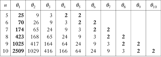
In §4, we focused on constraint C1 and the fact that its final weight grows exponentially with the number of constraints. We now focus instead on the last two constraints, C n−1 and C n . Table I shows that their weights always differ by just one at convergence. We can take advantage of this fact as follows. Let's train the learner on pristine data sampled from counterexample (9) until it converges to the final weights in Table I. At that point, we feed the learner just one corrupted piece of data such as (18): the violation difference corresponding to C1 is −1; the violation difference corresponding to the penultimate constraint, C n−1, is +1; the violation difference corresponding to the last constraint, C n , is +2; all other violation differences are null.
-
(18)

Since the violation difference corresponding to C1 is negative in (18) and the weight of C1 is very large in Table I, this corrupted piece of data is inconsistent with the weights in Table I, which are therefore updated to the weights in Table II, where the updated weights are given in bold. Because of the careful choice of the violation difference corresponding to the last two constraints, C n−1 and C n , they end up with the same weight, 2, in Table II. Consistency with the pristine training data in (9) requires the weight of C n−1 to be larger than the weight of C n . In order to recover the consistent weight configuration, the bottom row of counterexample (9) has to trigger an update. That update will promote C n−1 by 1, to weight 3. But constraints C n−2 and C n−1 will then have exactly the same weight, 3. Consistency with the pristine training data requires the weight of C n−2 to be larger than the weight of C n−1. As this reasoning can be repeated backward for all the constraints, we predict a domino effect.
Weights entertained by the truncated perceptron after the update triggered by the corrupted piece of data in (18).

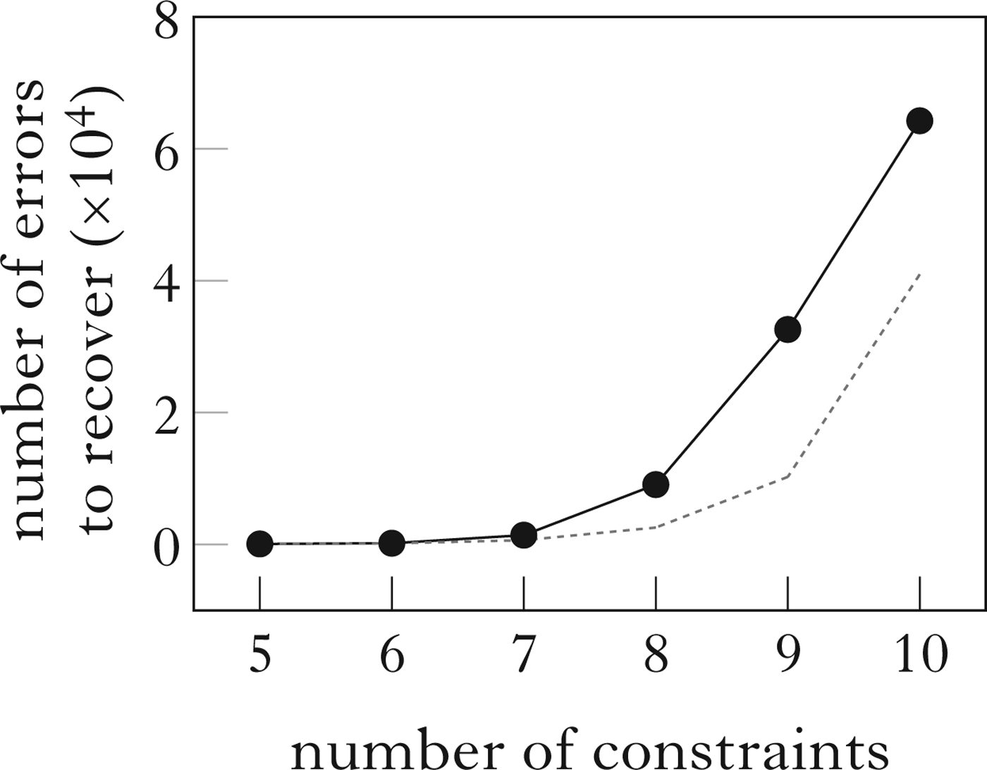
Indeed, the solid line in Fig. 13 plots the largest number of errors made by the HG learner (with the truncated perceptron reweighting rule) over ten runs on counterexample (9), starting from the weights in Table II (see Appendix E: Table XI for simulation results). Comparison with the function 40×4 n−5 plotted by the dashed line shows that the number of updates needed to recover from just a single small faulty update grows fast (exponentially) with the number of constraints, so fast that the learner requires over 64,000 updates in the case with just ten constraints, despite the weights in Table I and Table II before and after the faulty update being so similar.
Simulation results for the truncated perceptron in the noisy setting on counterexample (9).

In conclusion, this counterexample shows that constraint-independent guarantees of noise robustness for the HG error-driven learner are impossible, as a single faulty update can require a large number of updates to recover. Any such guarantees will have to be restricted by specific assumptions on the constraints.
6.2 Discussion
6.2.1 The margin, once again
Suppose that the HG learner is trained on a (possibly infinite) sequence of pristine training data generated by some target HG grammar interspersed with a finite amount of data corrupted by transmission noise or production errors. No assumptions are made on the corrupted data, apart from there being only a finite number. The number of errors made by the HG perceptron learner in this noisy learning setting is bounded by (19) (Freund & Schapire Reference Freund and Schapire1999, building on Klasner & Simon Reference Klasner, Simon and Maass1995; later developments such as Shalev-Shwartz & Singer Reference Shalev-Shwartz, Singer, Auer and Meir2005 and Mohri & Rostamizadeh Reference Mohri and Rostamizadeh2013 do not alter the shape of the bound). The precise definition of the quantity at the numerator of the second term of (19) is somewhat involved, and therefore omitted (for a description, see Magri Reference Magri2015). Suffice it to say that this quantity is null when there are no corrupted training data, and grows with the number of corrupted data. The error-bound extends to the truncated perceptron reweighting rule in (6), with the margin of the pristine data in the denominator replaced by the margin of the pristine + the dummy data (Magri Reference Magri2015).
-
(19)

This error-bound in (19) is the sum of two terms. The first term coincides with the error-bound in (10) for the (deterministic) HG learner in the noise-free setting. The second term thus quantifies the number of additional errors due to the corrupted data. This term depends on the number (and the shape) of the corrupted data through the numerator. It also depends on the margin of the pristine data through the denominator. As discussed in §4.3, the margin depends on the number of constraints. In the case of counterexample (9), its squared inverse grows fast (exponentially) with the number of constraints, as plotted in Fig. 8. The bound on the number of additional errors due to the noisy data thus grows fast, and does not settle question (d) in Fig. 4 concerning constraint-independent noise robustness. That question is answered negatively by the counterexample described in §6.1, which shows that constraint-independent guarantees for noise robustness are impossible in HG.
6.2.2 Comparison with OT
In the case of ten constraints, nine updates suffice for the OT learner to recover from the faulty update described in §6.1. These simulation results are not surprising. In fact, consider an OT learner which does not promote ‘too much’, i.e. one which adopts a promotion component (7a) corresponding to a calibration constant which is not ‘too large’, i.e. strictly smaller than 1. Suppose that the learner is trained on a (possibly infinite) sequence of data consistent with a certain OT grammar, interspersed with a finite number of corrupted data. The learner admits the error-bound in (20), which depends on the number of constraints, the calibration constant used in the definition of the promotion amount and the amount of corrupted training data (Magri Reference Magri2016).
-
(20)

This error-bound in (20) is the sum of two terms. The first term coincides with the error-bound in (12) for the noise-free setting. The second term thus expresses the number of additional errors due to the corrupted training data, and is in turn the product of the amount of corrupted data times a factor which quantifies the amount of disruption caused by each corrupted piece of data. This additional term grows slowly (linearly) with the number of constraints (as well as with the number of corrupted data). Furthermore, this bound requires no assumptions on the constraints. It thus answers question (d) in Fig. 4 concerning constraint-independent guarantees that the OT learner is robust to noise.
6.3 Summary
§4 and §5 compared the OT and HG implementations of error-driven learning in the noise-free setting. This section has extended the comparison to the noisy learning setting. It has focused on the number of additional errors made by the learner to recover from the faulty updates triggered by corrupted training data. The OT learner comes with a bound on the number of additional errors which provides constraint-independent guarantees on its noise robustness. The constraint-independent bound currently available for the HG learner instead does not guarantee noise robustness, because of its dependence on the margin of the data. Indeed, the HG learner is not noise robust constraint-independently: with just ten constraints, the HG learner can make more than 64,000 additional updates to recover from a faulty update triggered by a single piece of corrupted data.
7 Conclusions
The theories of OT and HG error-driven learning which emerge from the results presented in this paper are summarised in Figs 14 and 15, using the schema in Fig. 4. Various bounds for the OT learner have been considered which provide guarantees of convergence (is the number of errors finite?), efficiency (is the number of errors furthermore small?), stochastic tolerance (does the number of errors remain small in the stochastic implementation?) and noise robustness (does the number of errors remain small in the noisy setting?). These bounds follow from formal properties of the OT mode of constraint interaction and thus hold for any constraints. They provide positive answers to the four constraint-independent questions, which are therefore shaded in Fig. 14a–d. The four constraint-dependent questions in Fig. 14e–h become superfluous. The theory of OT error-driven learning has thus been successfully completed from a constraint-independent perspective.
OT theory of error-driven learning.

Various bounds for the perceptron HG learner (and their extensions to the truncated variant which ensures non-negative weights) have also been considered. They guarantee convergence irrespective of the constraints, and thus provide a positive answer to the constraint-independent question in Fig. 15a. The corresponding constraint-dependent question (e) thus becomes superfluous. Unfortunately, these bounds all depend on the margin of the data, a measure of the freedom in the choice of consistent weights. In §4.2, I described a class of cases where the margin decreases quickly with the number of constraints and the available bounds thus grow fast and provide no guarantees. Indeed, the HG learner has been shown not to converge efficiently in these cases, not to tolerate the stochastic implementation and not to be robust to noise. Constraint-independent guarantees are thus impossible for the HG learner, yielding a negative answer to the questions in Fig. 15b–d. Together, Figs 14 and 15 show that the theory of error-driven learning in OT and HG has a completely different nature (as foreshadowed in Prince & Smolensky Reference Prince and Smolensky2004: §10.2.2).
HG theory of error-driven learning.

The difference between OT and HG just established is best appreciated against the backdrop of a recent debate in computational phonology. Pater (Reference Pater2008) provides an elegant counterexample to Boersma's (Reference Boersma1998) GLA (Gradual Learning Algorithm) implementation of OT error-driven learning. He claims that ‘one reason for the failure [of the GLA on his counterexample], and potentially for its failure to provably converge in general, is its use of … OT as a model of grammar’ (2008: 341). He then notes that ‘the GLA closely resembles Rosenblatt's (Reference Rosenblatt1958) Perceptron’, which instead uses the HG model of grammar. He advocates the replacement of OT with HG and the adoption of the perceptron update rule for HG error-driven learning. Indeed, Pater (Reference Pater2009: 1021) argues that ‘one broad argument for weighted constraints … is that weighted constraints are compatible with existing well-understood algorithms for learning variable outcomes and for learning gradually’. The results summarised in Figs 14 and 15 turn this assessment on its head.
First, the problem with Pater's counterexample is not germane to the OT mode of constraint interaction. Rather, it is only due to a specific GLA implementation detail, namely the choice of a fixed promotion amount. As discussed in §4.3.2, the problem disappears if a promotion amount is adopted which is carefully calibrated, and in particular depends on the number of winner-preferring constraints, as prescribed by the promotion rule in (7a). Indeed, convergence, efficiency, stochastic tolerance and noise robustness are guaranteed for such an OT learner. And these guarantees hold independently of the phonological content of the constraints, circumventing the contentious issue of the characterisation of phonologically plausible constraints.
Second, the situation turns out to be very different for the HG learner. We have seen that the HG learner can make an astronomical number of errors: for instance, it makes more than 6,500,000 errors in counterexample (9), with just ten constraints. Hence, no constraint-independent efficiency guarantees are possible. Any HG efficiency guarantees will have to be restricted through proper assumptions on the constraints. The difficulty in developing such constraint-dependent analyses is that the behaviour of the HG learner can change abruptly in the face of even very small modifications of the training data. Indeed, we have seen that the number of errors drops to just 200 in the variant of the counterexample (9) considered in (14), despite the fact that the two test cases differ only minimally (changes in only two constraint-violation differences, by no more than 2). Finally, the behaviour of the HG learner can change abruptly if even small modifications of the current weights occur. Indeed, we have seen that a single, small update of the current weights (which changes only three weights by less than 2) has a dramatic effect, and requires the learner to perform over 64,000 additional updates to recover. These abrupt discontinuities in the behaviour of the HG learner in response to only small modifications of the data or the weights overturn Pater's assessment of the relative merits of OT and HG from the perspective of error-driven learning.
This conclusion in turn has implications for the connection between constraint-based phonology and the computational literature. There has been a rise of interest in learning with rankings in the recent machine learning literature (under the heading of preference learning; e.g. Fürnkranz & Hüllermeier Reference Fürnkranz and Hüllermeier2010). Because of its constraint-independent nature, the OT theory of error-driven learning is independent of the phonological substance, and might thus benefit from the methods and results developed within the computational literature. The HG theory must instead rely on substantive assumptions on the phonological content of specific constraints. In other words, the HG theory must focus on the implications for efficiency and robustness of subtle assumptions on phonologically plausible constraints. The machine learning literature has little to contribute to that enterprise. The HG theory of error-driven learning is thus unlikely to benefit from the analyses of general purpose ‘existing well-understood algorithms’ from the machine learning literature, contrary to Pater's suggestion (see for instance §4.3.7 above).
Of course, the choice between the OT and HG implementations of constraint-based phonology is an empirical issue, which should in the end be decided by typological considerations. However, recent research has started to compare the two frameworks from the perspective of their implications for acquisition and learnability (Riggle Reference Riggle2009, Bane et al. Reference Bane, Riggle and Sonderegger2010, Jesney & Tessier Reference Jesney and Tessier2011, Magri Reference Magri2013b). This paper has contributed to this line of research, through a re-evaluation of the relative merits of OT and HG from the perspective of error-driven learnability. The relevance of this re-evaluation can be concretely illustrated with the following example. Levelt et al. (Reference Levelt, Schiller and Levelt2000) report that Dutch-learning children go through acquisition stages where they allow a singly marked structure, while doubly marked structures lag behind. For instance, they allow syllables with complex codas and syllables with complex onsets, but not those where these two markedness violations gang up. Do these acquisition data show that child language displays gang-up effects and therefore requires HG over OT? The answer is unclear. Although, by design, OT does not capture gang-up effects, Jäger & Rosenbach (Reference Jäger and Rosenbach2006) show that some of these effects can be modelled in OT through the addition of a stochastic component. Building on this observation, Jarosz (Reference Jarosz2010) shows that stochastic OT is able to model the gang-up effects reported in Levelt's child data (with standard constraints for syllable types) and that an OT error-driven learner goes through intermediate stages which correspond to the attested gang-up effects. Which account of these gang-up effects is to be preferred, the stochastic OT account or the HG one? This is clearly a case where descriptive adequacy falls short. The computational results reported in this paper might help in this case. While the HG learner is not efficient from a constraint-independent perspective, the stochastic implementation does not affect the efficiency of the OT learner. These computational results might thus provide a starting point for a learnability-based argument which fills the gap left by the insufficiency of sheer phonological data.