1. Introduction
Inspection for faults of power grid components such as cables of the transmission and distribution system and insulators, as well as cleaning and de-icing of these components, is often carried out by humans [Reference Dian, Chen, Hoang, Pu and Liu1–Reference Wang and Wang7]. These are dangerous tasks, taking place in harsh conditions and exposing the life of the maintenance personnel to the risk of fatal accidents. To mitigate such risks and to perform faster and more efficient faults finding and repair in the power grid infrastructure, power-line inspection (PLI) robots can be used [Reference Park, Lee, Cho and Oh8–Reference Notomista, Emam and Egerstedm14]. The control problem of these robots remains a challenge because of the nonlinearities that characterize the related dynamic model and because of underactuation [Reference Yang, Feng, Sha and Ren15–Reference Wang, Yan, Pu, Xiang, Fan, Li and Zheng18]. So far, several approaches have been proposed for solving the nonlinear control problem of PLI robots [Reference Jiang, Yan, Yu, Peng, Li and Chen19–Reference Wang, Zhang, Jiang, Liu and Peng24]. Stability proof has become a prerequisite in the development of controllers for such robotic mechanisms [Reference Rigatos and Busawon25–Reference Guo, Mo and Song28]. Backstepping control and sliding mode control are among the nonlinear control methods one can consider for the PLI robots. However, such methods require the state-space model of the robots to be found in a specific form [Reference Rigatos and Busawon25]. Furthermore, there exist few results on the nonlinear optimal control of PLI robots and on how energy dissipation by their actuators can be reduced [Reference Menendez, Auat Cheein, Perez and Koura29, Reference Zhang, Liu, Fang and Wang30].
In this article, a novel nonlinear optimal (H-infinity) control method is developed for the dynamic model of an underactuated PLI robot [Reference Rigatos and Busawon25]. To this end, the robot’s dynamic model undergoes first approximate linearization around a time-varying operating point which is updated at each time step of the control method. Actually, at each sampling period, this operating point is defined by the present value of the robot’s state vector and by the last sampled value of the control inputs vector. The linearization relies on first-order Taylor series expansion and on the computation of the related Jacobian matrices [Reference Rigatos and Tzafestas31–Reference Rigatos and Zhang33]. The truncation of higher order terms from the Taylor series expansion is considered to be a perturbation that is asymptotically compensated by the robustness of the control method. For the approximately linearized model of the PLI robot, an optimal (H-infinity) feedback controller is designed.
The H-infinity controller provides the solution to the optimal control problem for the PLI robots under model uncertainty and external disturbances [Reference Rigatos34–Reference Rigatos, Siano, Wira and Profumo36]. It represents a min-max differential game taking place between (i) the control inputs which try to minimize a cost function that comprises a quadratic term of the state vector’s tracking error and (ii) the model uncertainty and external perturbations which try to maximize this cost function. To compute the stabilizing feedback gains of the H-infinity controller an algebraic Riccati equation is also solved at each sampling period of the control method [Reference Rigatos and Busawon25]. The stability properties of the control loop are proven through Lyapunov analysis. First, it is demonstrated that the control scheme satisfies the H-infinity tracking performance criterion [Reference Rigatos37, Reference Toussaint, Basar and Bullo38]. This signifies elevated robustness against model imprecision and exogenous perturbations. Moreover, under moderate conditions, it is proven that the control loop is globally asymptotically stable. Finally, to implement state estimation-based feedback control of the robot, without the need to measure its entire state vector, the H-infinity Kalman filter is used as a robust state estimator.
The necessity for using robotic systems for inspection and maintenance of the electricity grid is easy to understand since the related tasks expose the repair teams of power corporations to harsh and dangerous conditions with a high risk for fatal accidents [Reference Alhassan, Zhang, Shen and Xu5, Reference Rigatos and Busawon25]. Mainly, the following robotic systems are used for surveillance and repair of the electricity grid: (1) PLI robots suspended from cables, (2) unmanned micro-aerial vehicles, and (3) robotic manipulators and mobile manipulators with hydraulic or electric actuation. Robotic systems carrying out the inspection and maintenance of power lines are amenable to improvement and optimization of their function with respect to the following indicators: (i) precise positioning in the case of model uncertainty, accuracy in tasks execution, dexterity, and maneuverability, (ii) lower power consumption and higher autonomy and operational capacity, and (iii) reliability in underactuation conditions aiming at reduction of the robots’ weight and of their design’s complexity. With reference to (i) the article develops robust and fault-tolerant control and estimation methods that will preserve the reliable functioning of PLI robots. With reference to (ii) the article’s methods reduce energy consumption by PLI robots, thus improving their autonomy and operational capacity and reducing their functioning cost. With reference to (iii), the article’s findings allow to simplify the design of the robots used in power-lines inspection and maintenance and to reduce their weight and energy consumption, while also assuring that their accuracy in tasks execution, their maneuverability and their dexterity will remain unaffected.
A distinctive difference to previous results in this area is that the present article achieves a solution of the robot optimal control problem with global stability credentials and without model constraining assumptions. About [Reference Rigatos, Busawon, Pomares and Abbaszadeh39] it can be noted that the considered dynamic model of the 3-DOF wheel inverted pendulum robot is substantially different from the model of the power-lines inspection robot. Actually, the first robotic system exhibits three degrees of freedom and has two control inputs, while the model of the power-lines inspection robot has two degrees of freedom and receives only one control input. In ref. [Reference Beard and Mclain40], it is attempted to approximate the Hamilton–Jacobi–Bellman equation for the nonlinear optimal control problem with an expansion into Galerkin series. It remains to confirm the global stability properties of this control method and to verify its convergence to the solution of the nonlinear optimal control problem. In ref. [Reference Rahaghi and Barat41], a treatment of the nonlinear optimal control problem is attempted for nonlinear affine-in-the-input dynamical systems by assuming once again the decomposition of the solution of the Hamilton–Jacobi–Bellman equation into Galerkin series. It remains to prove global stability and to ensure convergence to the solution of the nonlinear optimal control problem. In ref. [Reference Siqueira and Terra42], a solution of the noninear optimal (H-infinity) control problem for cooperative robotic manipulators is attempted by assuming that the associated state-space model can be written in the linear parameter varying (LPV) form. The LPV assumption does not allow the application of the control method to systems which cannot be brought to the LPV form. In ref. [Reference Lin and Xin43] a state-dependent Riccati equation approach (SDRE) is proposed for the solution of the nonlinear optimal control problem in robotic systems. However, the application of the SDRE method is limited to systems which are found into the LPV form. In ref. [Reference Lin and Xin43], the use of robots for inspection of critical industrial installations, such as nuclear power plants, is considered. The proposed control scheme that is based on PID controllers may not assure global stability and reliable functioning under non-trivial operating conditions. In ref. [Reference Katrasnik, Pernus and Likar45], an overview is provided about the use of mobile robots in inspection tasks for the electric power transmission and distribution grid. It remains to demonstrate optimal control schemes that reduce energy consumption by such robots. Finally, in ref. [Reference Jiang, Ye, Zou and Yan46], mobile robots are proposed for the inspection of power lines in the MV-LV power distribution grid. It can be concluded that the nonlinear control problem of these robots and the associated solutions can be further developed.
The structure of the article is as follows: in Section 2, Euler-Lagrange analysis is applied, and the equations of motion of the PLI robot are obtained. The related state-space model is formulated. In Section 3, the state-space model of the robot undergoes approximate linearization with the use of Tayior series expansion and through the computation of the related Jacobian matrices. In Section 4, the global stability properties of the control scheme are proven through Lyapunov analysis. Furthermore, the H-infinity Kalman filter is presented as a robust state estimator for the PLI robot, which allows for implementing state estimation-based feedback control. Besides an H-infinity feedback controller is developed for the approximately linearized model of the robotic system. In Section 5, the differential flatness properties of the dynamic model of the PLI robot are analyzed and a flatness-based controller is developed for this robotic system. In Section 6, a sliding-mode controller is designed for the model of the power-lines inspection robot and the global stability properties of this control method are proven. In Section 7, the performance of the nonlinear optimal control method is further confirmed and evaluated through simulation experiments. Finally, in Section 8, concluding remarks are stated.
2. Dynamic Model of the PLI Robot
2.1. Computation of the robotic system’s Lagrangian
As noted above, one can distinguish three main classes of robotic systems used in the inspection and maintenance of the electricity grid: (1) autonomous robots that are suspended from cable lines, (2) unmanned aerial vehicles and aerial manipulators carrying out inspection tasks, and (3) mobile manipulators and robotic cranes involved also in faults finding and repair in the power grid infrastructure. As far as the first class of robotic systems is concerned, that is robots suspended from cable lines, one can distinguish mainly two-arm and multiarm robots [Reference Jiang, Zou, Zhou, Zuo, Cheng Ye and Li47–Reference Farias dos Santos, Abdali, Martins and Alexandre49]. As far as the second class of robotic systems is concerned that is unmanned aerial vehicles and aerial manipulators one can distinguish mainly autonomous helicopters, tricopters, quadropters, hexacopters, and octocopters [Reference Silano, Baca, Penicka, Liuzza and Saska50–Reference Guan, Sun, Su, Hu, Wang, Peng and Guo52]. These types of drones are often turned into aerial manipulators after attaching robotic arms on the aerial platforms. By incorporating robotic manipulators in these aerial platforms several types of unmanned aerial manipulators are obtained. As far as the third class of robotic systems is concerned that is mobile manipulators and robotic cranes once again one comes against several types of such types of robots (comprising different types of mobile platforms and multi-DOF robotic arms) [Reference Goncalves and Carvalho53, Reference Rigatos54].
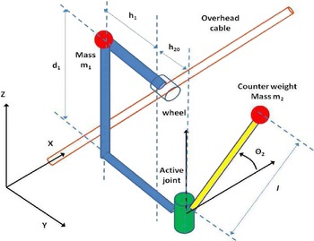
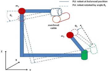
The specific type of the PLI robot to be analyzed next comes from [Reference Dian, Chen, Hoang, Pu and Liu1]. The diagram of the underactuated PLI robot is depicted in Figs. 1 and 2. Actually, in Fig. 2, it is considered that the PLI robot has been rotated about its vertical position by an angle
 $\theta_1$
. Then, in the OXYZ inertial reference frame, the coordinates of mass
 $m_1$
are
 $x_{m_1}=0$
,
 $y_{m_1}=-{h_1}cos(\theta_1)$
and
 $z_{m_1}=-{h_1}sin(\theta_1)$
. In the same reference frame, the coordinates of the counterweight mass
 $m_2$
are given by
 $x_{m_2}=lcos(\theta_2)$
,
 $y_{m_2}=(h_{20}-lsin(\theta_2))cos(\theta_1)+{d_1}sin(\theta_1)$
and
 $z_{m_2}=(h_{20}-lsin(\theta_2))sin(\theta_1)-{d_1}cos(\theta_1)$
.
Diagram of the PLI robot.

Rotation of the of the PLI robot by an angle
 $\theta_1$
from its balanced position and rotation of its counterweight mass
 $m_2$
by an angle
 $\theta_2.$

The velocity of mass
 $m_1$
is given by
 \begin{equation}\begin{array}{ccc}\dot{x}_{m_1}= 0\;\;\;\;\; & \dot{y}_{m_1}={h_1}sin(\theta_1))\dot{\theta}_1\;\;\;\;\; & z_{m_1}=-{h_1}cos(\theta_1))\dot{\theta}_1\end{array}\end{equation}
The velocity of mass
 $m_2$
is given by
 \begin{equation}\begin{array}{c}\displaystyle \dot{x}_{m_2}=-lsin(\theta_2)\dot{\theta}_2\\[5pt] \dot{y}_{m_2}=(\!-\!lcos(\theta_2)\dot{\theta}_2)cos(\theta_1)-(h_{20}-lsin(\theta_2))sin(\theta_1)\dot{\theta}_1+{d_1}cos(\theta_1)\dot{\theta}_1\\[5pt] \dot{z}_{m_2}=(\!-\!lcos(\theta_2)\dot{\theta}_2)sin(\theta_1)+(h_{20}-lsin(\theta_2))cos(\theta_1)\dot{\theta}_1+{d_1}sin(\theta_1)\dot{\theta}_1\end{array}\end{equation}
The kinetic energy due to translation of mass
 $m_1$
is
 \begin{equation}\begin{array}{c}\displaystyle K_1=\frac{1}{2}{m_1}\left(\dot{x}_{m_1}^2+\dot{y}_{m_1}^2+\dot{z}_{m_1}^2\right){\Rightarrow} \\[10pt] \displaystyle K_1=\frac{1}{2}{m_1}\left({h_1^2}sin^2\left(\theta_1\right)\dot{\theta}_1^2+{h_1^2}cos^2\left(\theta_1\right)\dot{\theta}_1^2\right){\Rightarrow}\\[10pt] \displaystyle K_1=\frac{1}{2}{m_1}{h_1^2}\dot{\theta}_1^2\end{array}\end{equation}
The kinetic energy due to translation of mass
 $m_2$
is
 \begin{equation}\begin{array}{c}\displaystyle K_2=\frac{1}{2}{m_2}\left(\dot{x}_{m_2}^2+\dot{y}_{m_2}^2\right)+\dot{z}_{m_2}^2{\Rightarrow} \\[8pt] \displaystyle K_2=\frac{1}{2}{m_2}\{{l^2}sin^2(\theta_2)\dot{\theta}_2^2+{l^2}cos^2(\theta_1)cos^2(\theta_2)\dot{\theta}_2^2\}+\\[10pt] \displaystyle +[(h_{20}-lsin(\theta_1)sin(\theta_1))-{d_1}cos(\theta_1)]^2\dot{\theta}_1^2-\\[5pt] \displaystyle -2[(\!-\!lcos(\theta_2))cos(\theta_1)][(h_{20}-lsin(\theta_2))sin(\theta_1)+{d_1}cos(\theta_1)]{\dot{\theta}_1}{\dot{\theta}_2}\\[5pt] \displaystyle +{l^2}cos^2(\theta_2)sin^2(\theta_1)\dot{\theta}_2^2+[(h_{20}-lsin(\theta_2))cos(\theta_1)+{d_1}sin(\theta)_1]^2\dot{\theta}_1^2+\\[5pt] \displaystyle +2[(\!-\!lcos(\theta_2))sin(\theta_1)][(h_{20}-lsin(\theta_2))cos(\theta_1)+{d_1}sin(\theta_1)]{\dot{\theta}_1}{\dot{\theta}_2}\end{array}\end{equation}
After regrouping terms, one obtains
 \begin{equation}\begin{array}{c}\displaystyle K_2=\frac{1}{2}m_2\{{l^2}sin^2(\theta_2)\dot{\theta}_2^2+{l^2}cos^2(\theta_2)\dot{\theta}_2^2+\\[8pt] \displaystyle (h_{20}-lsin(\theta_2))^2\dot{\theta}_1^2+{d_1^2}\dot{\theta}_1^2-\\[5pt] \displaystyle -2(\!-\!lcos(\theta_2))cos(\theta_1)(h_{20}-lsin(\theta_2))sin(\theta_1){\dot{\theta}_1}{\dot{\theta}_2}-\\[5pt] \displaystyle -2(lcos(\theta_2))cos(\theta_1){d_1}cos(\theta_1){\dot{\theta}_1}{\dot{\theta}_2}+\\[5pt] \displaystyle +2(lcos(\theta_2))sin(\theta_1)(h_{20}-lsin(\theta_2))cos(\theta_1){\dot{\theta}_1}{\dot{\theta}_2}+\\[5pt] \displaystyle +2(lcos(\theta_2))sin(\theta_1){d_1}cos(\theta_1){\dot{\theta}_1}{\dot{\theta}_2}\}\end{array}\end{equation}
Through additional operations, one obtains
 \begin{equation}\begin{array}{c}\displaystyle K_2=\frac{1}{2}m_2\left\{{l^2}{\dot{\theta}_2^2}+(h_{20}-lsin(\theta_1))^2{\dot{\theta}_1^2}+{d_1^2}\dot{\theta}_1^2\right\}\end{array}\end{equation}
Therefore, the total kinetic energy of the robotic mechanism is
 \begin{equation}\begin{array}{c}\displaystyle K=K_1+K_2{\Rightarrow} \\[5pt] \displaystyle K=\frac{1}{2}{m_1}{h_1^2}\dot{\theta}_1^2+\frac{1}{2}{m_2}{l^2}\dot{\theta}_2^2+\frac{1}{2}{m_2}\left[(h_{20}-lsin(\theta_1))^2+d_1^2\right]\dot{\theta}_1^2\end{array}\end{equation}
Next, the potential energy of the robotic mechanism is computed. The potential energy of mass
 $m_1$
is
 \begin{equation}\begin{array}{c}\displaystyle P_1={m_1}g{z_1}{\Rightarrow}{P_1}={m_1}g(-{h_1}sin(\theta_1))\\[5pt] \displaystyle {\Rightarrow}{P_1}=-{m_1}g{h_1}sin(\theta_1)\end{array}\end{equation}
The potential energy of mass
 $m_2$
is
 \begin{equation}\begin{array}{c}\displaystyle P_2={m_2}g{z_2}{\Rightarrow}{P_2}={m_2}g[(h_{20}-lsin(\theta_2))sin(\theta_1)-{d_1}cos(\theta_1)]\\[5pt] \displaystyle {\Rightarrow}{P_1}=-{m_1}g{h_1}sin(\theta_1)\end{array}\end{equation}
The aggregate potential energy of the robotic system is given by
 \begin{equation}\begin{array}{c}\displaystyle P={P_1}+{P_2}{\Rightarrow} \\[5pt]\displaystyle P=-{m_1}g{h_1}sin(\theta_1)-{m_2}g[(h_{20}-lsin(\theta_2))sin(\theta_1)-{d_1}cos(\theta_1)]\end{array}\end{equation}
the Lagrangian of the robotic system is [Reference Dian, Chen, Hoang, Pu and Liu1, Reference Rigatos and Busawon25]
 \begin{equation}\begin{array}{c}\displaystyle L=K-P{\Rightarrow} \\[5pt] \displaystyle L=\frac{1}{2}{m_1}{h_1^2}\dot{\theta}_1^2+\frac{1}{2}{m_2}{l^2}\dot{\theta}_2^2+\frac{1}{2}{m_2}\left[(h_{20}-lsin(\theta_1))^2+d_1^2\right]\dot{\theta}_1^2+\\[9pt] \displaystyle +{m_1}g{h_1}sin(\theta_1)+{m_2}g\left[(h_{20}-lsin(\theta_2))sin(\theta_1)-{d_1}cos(\theta_1)\right]\end{array}\end{equation}
2.2. State-space model of the PLI robot
The equations that constitute the dynamic model of the power-line inspection robot are obtained from the related Euler–Lagrange equations:
 \begin{equation}\begin{array}{c}\displaystyle {{\partial} \over {{\partial}t}}{{{\partial}L} \over {{\partial}\dot{\theta}_1}}-{{{\partial}L} \over {{\partial}\theta_1}}=0\\ \\\displaystyle {{\partial} \over {{\partial}t}}{{{\partial}L} \over {{\partial}\dot{\theta}_2}}-{{{\partial}L} \over{{\partial}\theta_2}}=u\end{array}\end{equation}
where u is the torque applied to the actuator of the joint that rotates the counterweight of mass
 $m_2$
. It holds that
 \begin{equation}\begin{array}{c}\displaystyle {{{\partial}L} \over {{\partial}\dot{\theta}_1}}={m_1}{h_1^2}{\dot{\theta}_1}+{m_2}[(h_{20}-lsin(\theta_2))^2+{d_1^2}]{\dot{\theta}_1}\end{array}\end{equation}
Moreover, it holds that
 \begin{equation}\begin{array}{c}\displaystyle {d \over {dt}}{{{\partial}L} \over {{\partial}\dot{\theta}_1}}={m_1}{h_1^2}\ddot{\theta}_1+{m_2}\left[2(h_{20}-lsin(\theta_2))(\!-\!lcos(\theta_2))\dot{\theta}_2\right]\dot{\theta}_1+\\[8pt] \displaystyle +{m_2}\left[(h_{20}-lsin(\theta_2))^2+{d_1^2}\right]\ddot{\theta}_1{\Rightarrow}\\[5pt]\displaystyle {d \over {dt}}{{{\partial}L} \over {{\partial}\dot{\theta}_1}}=\left\{{m_1}{h_1^2}+{m_2}\left[(h_{20}-lsin(\theta_2))^2+{d_1^2}\right]\right\}\ddot{\theta}_1+\\[8pt] \displaystyle +{m_2}\left[2(h_{20}-lsin(\theta_2))(\!-\!lcos(\theta_2))\right]{\dot{\theta}_1}{\dot{\theta}_2}\end{array}\end{equation}
Additionally, one has that
 \begin{equation}\begin{array}{c}\displaystyle {{{\partial}L} \over {{\partial}{\theta}_1}}={m_1}g{{h_1}cos(\theta_1)}-{m_2}g[(h_{20}-lsin(\theta_2))cos(\theta_1)+{d_1}sin(\theta_1)]\end{array}\end{equation}
Consequently, the first equation of motion becomes
 \begin{equation}\begin{array}{c}\displaystyle {{\partial} \over {{\partial}t}}{{{\partial}L} \over {{\partial}\dot{\theta}_1}}-{{{\partial}L} \over {{\partial}\theta_1}}=0{\Rightarrow} \\[9pt] \displaystyle \left\{{m_1}{h_1^2}+{m_2}\left[(h_{20}-lsin(\theta_2))^2+{d_1^2}\right]\right\}\ddot{\theta}_1+\\[5pt] \displaystyle +{m_2}\left[2(h_{20}-lsin(\theta_2))(\!-\!lcos(\theta_2))\right]{\dot{\theta}_1}{\dot{\theta}_2}-\\[5pt] \displaystyle -{m_1}g{{h_1}cos(\theta_1)}+{m_2}g\left[(h_{20}-lsin(\theta_2))cos(\theta_1)+{d_1}sin(\theta_1)\right]=0\end{array}\end{equation}
Furthermore, one has
 \begin{equation}\begin{array}{c}\displaystyle {{{\partial}L} \over {{\partial}\dot{\theta}_2}}={m_2}{l^2}\dot{\theta}_2\end{array}\end{equation}
and also
 \begin{equation}\begin{array}{c}\displaystyle {d \over {dt}}{{{\partial}L} \over {{\partial}\dot{\theta}_2}}={m_2}{l^2}\ddot{\theta}_2\end{array}\end{equation}
Moreover, it holds that
 \begin{equation}\begin{array}{c}\displaystyle {{{\partial}L} \over {{\partial}{\theta}_2}}={m_2}(h_{20}-lsin(\theta_2))(\!-\!lcos(\theta_2))\dot{\theta}_1^2-{m_2}g(\!-\!lcos(\theta_2))sin(\theta_1)\end{array}\end{equation}
Thus, the second equation of motion of the robotic system becomes
 \begin{equation}\begin{array}{c}\displaystyle {{\partial} \over {{\partial}t}}{{{\partial}L} \over {{\partial}\dot{\theta}_2}}-{{{\partial}L} \over {{\partial}\theta_2}}=u{\Rightarrow}\\[9pt] m{l^2}\ddot{\theta}_2+{m_2}(h_{20}-lsin(\theta_2))(lcos(\theta_2))\dot{\theta}_1^2-{m_2}g(lcos(\theta_2))sin(\theta_1)=u\end{array}\end{equation}
The following state variables are defined:
 $x_1=\theta_1$
,
 $x_2=\dot{\theta}_1$
,
 $x_3=\theta_2$
and
 $x_4=\dot{\theta}_2$
. Consequently, one can obtain the following state-space description:
 \begin{equation}\begin{array}{c}\displaystyle \left\{{m_1}{h_1^2}+{m_2}[(h_{20}-lsin(x_3))^2+{d_1^2}]\right\}\ddot{x}_1+{m_2}\left[2(h_{20}-lsin(x_3))(\!-\!lcos(x_3))\right]{x_2}{x_4}-\\[5pt]\displaystyle -{m_1}g{h_1}cos(x_1)+{m_2}g\left[(h_{20}-lsin(x_3))cos(x_1)+{d_1}sin(x_1)\right]=0\end{array}\end{equation}
 \begin{equation}\begin{array}{c}\displaystyle {m_2}{l^2}\ddot{x}_3+{m_2}(h_{20}-lsin(x_3))lcos(x_3){x_2^2}-{m_1}g(lcos(x_3))sin(x_1)=u\end{array}\end{equation}
The previous state-space model can be also written as
 \begin{equation}\ddot{x}_1={{{m_2}[2(h_{20}-lsin(x_3))(lcos(x_3))]{x_2}{x_4}} \over {\{{m_1}{h_1^2}+{m_2}[(h_{20}-lsin(x_3))^2+]\}}}+{{{m_1}g{h_1}cos(x_1)+{m_2}g[(h_{20}-lsin(x_3))cos(x_1)+{d_1}sin(x_1)]} \over {\{{m_1}{h_1^2}+{m_2}[(h_{20}-lsin(x_3))^2]\}}}\end{equation}
 \begin{equation}\ddot{x}_3={{-{m_2}(h_{20}-lsin(x_3))lcos(x_3){x_2^2}+{m_1}g(lcos(x_3))sin(x_1)} \over {{m_2}{l^2}}}+{u \over {{m_2}{l^2}}}\end{equation}
Additionally, the state-space model of the system can be written as
 \begin{equation}\dot{x}_1=x_2\end{equation}
 \begin{equation}\dot{x}_2={{{m_2}[2(h_{20}-lsin(x_3))(lcos(x_3))]{x_2}{x_4}} \over {\{{m_1}{h_1^2}+{m_2}[(h_{20}-lsin(x_3))^2+]\}}}+{{{m_1}g{h_1}cos(x_1)+{m_2}g[(h_{20}-lsin(x_3))cos(x_1)+{d_1}sin(x_1)]} \over {\{{m_1}{h_1^2}+{m_2}[(h_{20}-lsin(x_3))^2]\}}}\end{equation}
 \begin{equation}\dot{x}_3=x_4\end{equation}
 \begin{equation}\dot{x}_4={{-{m_2}(h_{20}-lsin(x_3))lcos(x_3){x_2^2}+{m_1}g(lcos(x_3))sin(x_1)} \over {{m_2}{l^2}}}+{u \over {{m_2}{l^2}}}\end{equation}
Furthermore, one can consider the following concise description of the system in vector fields form
 \begin{equation}\dot{x}=f(x)+g(x)u\end{equation}
where
 $x{\in}R^{4{\times}1}$
,
 $f(x){\in}R^{4{\times}1}$
and
 $g(x){\in}R^{4{\times}1}$
while
 $u{\in}R$
, or equivalently
 \begin{equation}\begin{array}{c}\displaystyle \begin{pmatrix}\dot{x}_1 \\[5pt] \dot{x}_2 \\[5pt] \dot{x}_3 \\[5pt] \dot{x}_4\end{pmatrix}=\begin{pmatrix}f_1(x) \\[5pt] f_2(x) \\[5pt] f_3(x) \\[5pt] f_4(x)\end{pmatrix}+\begin{pmatrix}g_1(x) \\[5pt] g_2(x) \\[5pt] g_3(x) \\[5pt] g_4(x)\end{pmatrix}u\end{array}\end{equation}
where
 $f_1(x)=x_2$
,
 $f_2(x)={\frac{{m_2}[2(h_{20}-lsin(x_3))(lcos(x_3))]{x_2}{x_4}}{\{{m_1}{h_1^2}+{m_2}[(h_{20}-lsin(x_3))^2+]\}}}+{{{m_1}g{h_1}cos(x_1)+{m_2}g[(h_{20}-lsin(x_3))cos(x_1)+{d_1}sin(x_1)]} \over {\{{m_1}{h_1^2}+{m_2}[(h_{20}-lsin(x_3))^2]\}}}$
 $f_3(x)=x_4$
,
 $f_4(x)={{f_{4n}(x)} \over {f_{4d}(x)}}={{-{m_2}(h_{20}-lsin(x_3))lcos(x_3){x_2^2}+{m_1}g(lcos(x_3))sin(x_1)} \over {{m_2}{l^2}}}$
and
 $g_1(x)=0$
,
 $g_2(x)=0$
,
 $g_3(x)=0$
and
 $g_4(x)={1 \over {{m_2}{l^2}}}$
.
3. Approximate Linearization of the Power-line Inspection Robot
3.1. Approximately linearized model
The dynamic model of the PLI robot
 $\dot{x}=f(x)+g(x)u$
undergoes approximate linearization around the time-varying operating point
 $(x^{*},u^{*})$
, where
 $x^{*}$
is the present value of the system’s state vector and
 $u^{*}$
is the last sampled value of the control inputs vector. The linearization relies on first-order Taylor series expansion and on the computation of the related Jacobian matrices.
This concept results into the approximately linearized model of the robotic system in the form:
 \begin{equation}\begin{array}{c}\displaystyle \dot{x}=Ax+Bu+\tilde{d}\end{array}\end{equation}
where
 $\tilde{d}$
is the cumulative perturbations’ vector which comprises (i) the modeling error due to truncation of higher-order terms in the Taylor series expansion, (ii) external disturbances, and (iii) measurement noise of any distribution.
The Jacobian matrices of the robotic system are
 \begin{equation}\begin{array}{c}\displaystyle A={\nabla_x}[f(x)+g(x)u]\mid_{(x^{*},u^{*})}{\Rightarrow}A={\nabla_x}[f(x)]\mid_{(x^{*},u^{*})}+{\nabla_x}[g(x)]u\mid_{(x^{*},u^{*})}{\Rightarrow}\\[5pt] \displaystyle A={\nabla_x}[f(x)]\mid_{(x^{*},u^{*})}\end{array}\end{equation}
 \begin{equation}\begin{array}{c}\displaystyle B={\nabla_u}[f(x)+g(x)u]\mid_{(x^{*},u^{*})}{\Rightarrow}B=g(x)\mid_{(x^{*},u^{*})}\end{array}\end{equation}
Next, the elements of the Jacobian matrix
 ${\nabla_x}[f(x)]\mid_{(x^{*},u^{*})}$
are computed.
First row of the Jacobian matrix
 ${\nabla_x}[f(x)]\mid_{(x^{*},u^{*})}$
:
 ${{{\partial}{f_1}} \over {{\partial}{x_1}}}=0$
,
 ${{{\partial}{f_1}} \over {{\partial}{x_2}}}=1$
,
 ${{{\partial}{f_1}} \over {{\partial}{x_3}}}=0$
and
 ${{{\partial}{f_1}} \over {{\partial}{x_4}}}=0$
.
Second row of the Jacobian matrix
 ${\nabla_x}[f(x)]\mid_{(x^{*},u^{*})}$
: for
 $i=1,\cdots,4$
 \begin{equation}{{{\partial}f_2} \over {{\partial}{x_i}}}={\frac{{{\partial}f_{2n}(x) \over \partial{x_i}}f_{2d}(x)-f_{2n}(x){{{\partial}f_{2d}(x)} \over \partial{x_i}}}{{f_{2d}(x)}^2}}\end{equation}
where
 ${{{\partial}f_{2n}} \over {{\partial}x_1}}={m_1}g{h_1}(-sin(x_1))+{m_2}g[-(h_{20}+lsin(x_3))sin(x_1)+{d_1}cos(x_1)]$
,
 $ {{{\partial}f_{2n}} \over {{\partial}x_2}}={m_2}[2(h_{20}-lsin(x_3)) (lcos(x_3))]x_4$
,
 ${{{\partial}f_{2n}} \over {{\partial}x_3}}=2{m_2}[(\!-\!lcos(x_3))(lcos(x_3))]{x_2}{x_4}-2{m_2}(h_{20}-lsin(x_3))(lsin(x_3)){x_2}{x_4}+{m_2}g[(lcos(x_3)) cos(x_1)]$
,
 ${{{\partial}f_{2n}} \over {{\partial}x_4}}={m_2}[2(h_{20}-lsin(x_3))(lcos(x_3))]x_2$
.
and also
 ${{{\partial}f_{2d}} \over {{\partial}x_1}}=0$
,
 ${{{\partial}f_{2d}} \over {{\partial}x_12}}=0$
,
 ${{{\partial}f_{2d}} \over {{\partial}x_3}}={m_2}2(h_{20}-lsin(x_3))(\!-\!lcos(x_3))$
,
 ${{{\partial}f_{2d}} \over {{\partial}x_4}}=0$
.
Third row of the Jacobian matrix
 ${\nabla_x}[f(x)]\mid_{(x^{*},u^{*})}$
:
 ${{{\partial}{f_3}} \over {{\partial}{x_1}}}=0$
,
 ${{{\partial}{f_3}} \over {{\partial}{x_2}}}=0$
,
 ${{{\partial}{f_3}} \over {{\partial}{x_3}}}=0$
and
 ${{{\partial}{f_3}} \over {{\partial}{x_4}}}=1$
.
Fourth row of the Jacobian matrix
 ${\nabla_x}[f(x)]\mid_{(x^{*},u^{*})}$
:
 ${{{\partial}f_4(x)} \over {{\partial}x_1}}={1 \over {{m_2}l^2}}({m_2}g(lcos(x_3))cos(x_1))$
,
 ${{{\partial}f_4(x)} \over {{\partial}x_2}}=-{2{x_2} \over {{m_2}l^2}}$
,
 ${{{\partial}f_4(x)} \over {{\partial}x_3}}={1 \over {{m_2}l^2}}[-{m_2}(\!-\!lcos(x_3))(lcos(x_3)){x_2^2}-{m_2}(h_{20}-lsin(x_3))(\!-\!lsin(x_3)){x_2^2}-{m_2}g(lsin(x_3))sin(x_1)]$
, and
 ${{{\partial}f_4(x)} \over {{\partial}x_3}}=0$
3.2. Stabilizing feedback control
After linearization around its current operating point, the dynamic model of the PLI robot is written as
 \begin{equation}\begin{array}{c}\displaystyle \dot{x}=Ax+Bu+d_1\end{array}\end{equation}
Parameter
 $d_1$
stands for the linearization error in the PLI robot’s dynamic model appearing previously in Eq. (31). The reference setpoints for the PLI robot’s state vector are denoted by
 ${\bf{x_d}}=[x_1^{d},\cdots,x_4^{d}]$
. Tracking of this trajectory is achieved after applying the control input
 $u_d$
. At every time instant, the control input
 $u_d$
is assumed to differ from the control input u appearing in Eq. (35) by an amount equal to
 ${\Delta}u$
, that is
 $u_d=u+{\Delta}u$
 \begin{equation}\begin{array}{c}\displaystyle \dot{x}_d=Ax_d+Bu_d+d_2\end{array}\end{equation}
The dynamics of the controlled system described in Eq. (35) can be also written as
 \begin{equation}\begin{array}{c}\displaystyle \dot{x}=Ax+Bu+Bu_d-Bu_d+d_1\end{array}\end{equation}
and by denoting
 $d_3=-Bu_d+d_1$
as an aggregate disturbance term one obtains
 \begin{equation}\begin{array}{c}\displaystyle \dot{x}=Ax+Bu+Bu_d+d_3\end{array}\end{equation}
By subtracting Eq. (36) from Eq. (38) one has
 \begin{equation}\begin{array}{c}\displaystyle \dot{x}-\dot{x}_d=A(x-x_d)+Bu+d_3-d_2\end{array}\end{equation}
By denoting the tracking error as
 $e=x-x_d$
and the aggregate disturbance term as
 $\tilde{d}=d_3-d_2$
, the tracking error dynamics becomes
 \begin{equation}\begin{array}{c}\displaystyle \dot{e}=Ae+Bu+\tilde{d}\end{array}\end{equation}
For the approximately linearized model of the system a stabilizing feedback controller is developed. The controller has the form
 \begin{equation}\begin{array}{c}\displaystyle u(t)=-Ke(t)\end{array}\end{equation}
with
 $K={1 \over r}{B^T}P$
where P is a positive definite symmetric matrix which is obtained from the solution of the Riccati equation [Reference Rigatos and Busawon25]
 \begin{align}{A^T}P+PA+Q-P\left({2 \over r}B{B^T}-{1 \over {\rho^2}}L{L^T}\right)P=0\end{align}
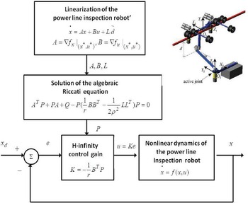
where Q is a positive semi-definite symmetric matrix. The diagram of the considered control loop is depicted in Fig. 3. Clear metrics can be provided about the robustness properties of the proposed nonlinear optimal (H-infinity) control scheme for PLI robots. The solution of the H-infinity feedback control problem for the underactuated PLI robot and the computation of the worst case disturbance that the related controller can sustain, comes from superposition of Bellman’s optimality principle when considering that the robot is affected by two separate inputs (i) the control input u (ii) the cumulative disturbance input
 $\tilde{d}(t)$
. Solving the optimal control problem for u, that is for the minimum variation (optimal) control input that achieves elimination of the state vector’s tracking error, gives
 $u=-{1 \over r}{B^T}Pe$
. Equivalently, solving the optimal control problem for
 $\tilde{d}$
, that is for the worst case disturbance that the control loop can sustain gives
 $\tilde{d}={1 \over \rho^2}{L^T}Pe$
. The attenuation coefficient
 $\rho$
can be given a small value up to the point that the method’s algebraic Riccati equation still returns a valid solution in the form of the positive definite and symmetric matrix P. The smallest value of
 $\rho$
for which a valid solution of the method’s algebraic Riccati equation can be obtained (in the form of a positive definite and symmetric matrix P) is the one that provides maximum robustness to the control loop.
Diagram of the control scheme for the power-line inspection robot (the figure of the PLI robot comes from [Reference Dian, Chen, Hoang, Pu and Liu1])

The present article provides one of the few existing solutions to the nonlinear optimal control problem of PLI robots which is of proven global stability while also remaining computationally efficient. Preceding results on the use of H-infinity control to nonlinear dynamical systems were limited to the case of affine-in-the-input systems with drift-only dynamics and considered that the control inputs gain matrix is not dependent on the values of the system’s state vector. Moreover, in these approaches, the linearization was performed around points of the desirable trajectory, whereas in the present article’s control method the linearization points are related with the value of the state vector at each sampling instance as well as with the last sampled value of the control inputs vector. The Riccati equation which has been proposed for computing the feedback gains of the controller is novel, so is the presented global stability proof through Lyapunov analysis. The article’s approach enables a solution of the nonlinear optimal control problem without the need to solve state dependent Riccati equations (SDREs).
The article’s scientific contribution is outlined as follows: (i) the presented nonlinear optimal control method has improved performance when compared against other nonlinear control schemes that one can consider for the dynamic model of the PLI robots (such as Lie algebra-based control, differential flatness theory-based control, model-based predictive control, nonlinear model-based predictive control, sliding-mode control, backstepping control), etc., (ii) it achieves fast and accurate tracking of all reference setpoints for the PLI robots under moderate variations of the control inputs, and (iii) it minimizes the consumption of energy by the actuators of the PLI robots, thus improving the functioning cost and efficiency in tasks’ execution by such robotic systems.
4. Lyapunov Stability Analysis
4.1. Stability proof
Through Lyapunov stability analysis, it will be shown that the proposed nonlinear optimal control scheme, which was formulated in Section 3, assures
 $H_{\infty}$
tracking performance for the underactuated PLI robot and that in case of bounded disturbance terms asymptotic convergence to the reference setpoints is achieved. The tracking error dynamics for the PLI robot is written in the form [Reference Rigatos and Busawon25]
 \begin{equation}\begin{array}{c}\displaystyle \dot{e}=Ae+Bu+L\tilde{d}\end{array}\end{equation}
where in the PLI robot’s case
 $L{\in}R^{4{\times}4}$
is the disturbance inputs gain matrix. Variable
 $\tilde{d}$
denotes model uncertainties and external disturbances of the PLI robot’s model. The following Lyapunov equation is considered
 \begin{equation}\begin{array}{c}\displaystyle V=\frac{1}{2}{e^T}Pe\end{array}\end{equation}
where
 $e=x-x_d$
is the tracking error. By differentiating with respect to time one obtains
 \begin{equation}\begin{array}{c}\displaystyle \dot{V}=\frac{1}{2}{\dot{e}^T}Pe+\frac{1}{2}{e^T}P\dot{e}{\Rightarrow}\\[9pt] \displaystyle \dot{V}=\frac{1}{2}{\big[Ae+Bu+L\tilde{d}\big]^T}Pe+\frac{1}{2}{e^T}P\big[Ae+Bu+L\tilde{d}\big]{\Rightarrow} \\[5pt] \end{array}\end{equation}
 \begin{equation}\begin{array}{c}\displaystyle \dot{V}=\frac{1}{2}\big[{e^T}{A^T}+{u^T}{B^T}+{\tilde{d}^T}{L^T}\big]Pe+\\[9pt] \displaystyle +\frac{1}{2}{e^T}P\big[Ae+Bu+L\tilde{d}\big]{\Rightarrow} \\[5pt] \end{array}\end{equation}
 \begin{equation}\begin{array}{c}\displaystyle \dot{V}=\frac{1}{2}{e^T}{A^T}Pe+\frac{1}{2}{u^T}{B^T}Pe+\frac{1}{2}{\tilde{d}^T}{L^T}Pe+ \\[9pt] \displaystyle \frac{1}{2}{e^T}PAe+\frac{1}{2}{e^T}PBu+\frac{1}{2}{e^T}PL\tilde{d}\end{array}\end{equation}
The previous equation is rewritten as
 \begin{equation}\begin{array}{c}\displaystyle \dot{V}=\frac{1}{2}{e^T}\left({A^T}P+PA\right)e+\left(\frac{1}{2}{u^T}{B^T}Pe+\frac{1}{2}{e^T}PBu\right)+\\[8pt] \displaystyle +\left(\frac{1}{2}{\tilde{d}^T}{L^T}Pe+\frac{1}{2}{e^T}PL\tilde{d}\right)\end{array}\end{equation}
Assumption: For given positive definite matrix Q and coefficients r and
 $\rho$
there exists a positive definite matrix P, which is the solution of the following matrix equation
 \begin{equation}\begin{array}{c}\displaystyle {A^T}P+PA=-Q+P\left({2 \over r}B{B^T}-{1 \over \rho^2}L{L^T}\right)P\end{array}\end{equation}
Moreover, the following feedback control law is applied to the system
 \begin{equation}\begin{array}{c}\displaystyle u=-{1 \over {r}}{B^T}Pe\end{array}\end{equation}
By substituting Eqs. (49) and (50), one obtains
 \begin{equation}\begin{array}{c}\displaystyle \dot{V}=\frac{1}{2}{e^T}\left[-Q+P\left({2 \over r}B{B^T}-{1 \over \rho^2}L{L^T}\right)P\right]e+\\[11pt] \displaystyle +{e^T}PB\left(-{1 \over {r}}{B^T}Pe\right)+{e^T}PL\tilde{d}{\Rightarrow}\end{array}\end{equation}
 \begin{equation}\begin{array}{c}\displaystyle \dot{V}=-\frac{1}{2}{e^T}Qe+{1 \over {r}}{e^T}PB{B^T}Pe-{1 \over {2\rho^2}}{e^T}PL{L^T}Pe\\[8pt]\displaystyle -{1 \over {r}}{e^T}PB{B^T}Pe+{e^T}PL\tilde{d}\end{array}\end{equation}
which after intermediate operations gives
 \begin{equation}\begin{array}{c}\displaystyle \dot{V}=-\frac{1}{2}{e^T}Qe-{1 \over {2\rho^2}}{e^T}PL{L^T}Pe+{e^T}PL\tilde{d}\end{array}\end{equation}
or, equivalently
 \begin{equation}\begin{array}{c}\displaystyle \dot{V}=-\frac{1}{2}{e^T}Qe-{1 \over {2\rho^2}}{e^T}PL{L^T}Pe+\\[9pt] \displaystyle +\frac{1}{2}{e^T}PL\tilde{d}+\frac{1}{2}{\tilde{d}^T}{L^T}Pe\end{array}\end{equation}
Lemma: The following inequality holds
 \begin{equation}\begin{array}{c}\displaystyle \frac{1}{2}{e^T}L\tilde{d}+\frac{1}{2}\tilde{d}{L^T}Pe-{1 \over {2\rho^2}}{e^T}PL{L^T}Pe{\leq}{1 \over2}{\rho^2}{\tilde{d}^T}\tilde{d}\end{array}\end{equation}
Proof: The binomial
 $({\rho}{\alpha}-{1 \over \rho}b)^2$
is considered. Expanding the left part of the above inequality one gets
 \begin{equation}\begin{array}{c}\displaystyle {\rho^2}{a^2}+{1 \over {\rho^2}}{b^2}-2ab \geq 0 \Rightarrow {1\over 2}{\rho^2}{a^2}+{1 \over {2\rho^2}}{b^2}-ab \geq 0 \Rightarrow\\[5pt] \displaystyle ab-{1 \over {2\rho^2}}{b^2} \leq \frac{1}{2}{\rho^2}{a^2}\Rightarrow \frac{1}{2}ab+\frac{1}{2}ab-{1 \over {2\rho^2}}{b^2}\leq \frac{1}{2}{\rho^2}{a^2}\end{array}\end{equation}
The following substitutions are carried out:
 $a=\tilde{d}$
and
 $b={e^T}{P}L$
and the previous relation becomes
 \begin{equation}\begin{array}{c}\displaystyle \frac{1}{2}{\tilde{d}^T}{L^T}Pe+\frac{1}{2}{e^T}PL\tilde{d}-{1 \over {2\rho^2}}{e^T}PL{L^T}Pe{\leq}\frac{1}{2}{\rho^2}\tilde{d}^T\tilde{d}\end{array}\end{equation}
Eq. (57) is substituted in Eq. (54) and the inequality is enforced, thus giving
 \begin{equation}\begin{array}{c}\displaystyle \dot{V}{\leq}-\frac{1}{2}{e^T}Qe+\frac{1}{2}{\rho^2}{\tilde{d}^T}\tilde{d}\end{array}\end{equation}
Eq. (58) shows that the
 $H_{\infty}$
tracking performance criterion is satisfied. The integration of
 $\dot{V}$
from 0 to T gives
 \begin{equation}\begin{array}{c}\displaystyle {\int_0^T}\dot{V}(t)dt{\leq}-\frac{1}{2}{\int_0^T}{||e||_Q^2}{dt}+\frac{1}{2}{\rho^2}{\int_0^T}{||\tilde{d}||^2}{dt}{\Rightarrow}\\[9pt] \displaystyle 2V(T)+{\int_0^T}{||e||_Q^2}{dt}{\leq}2V(0)+{\rho^2}{\int_0^T}{||\tilde{d}||^2}dt\end{array}\end{equation}
Moreover, if there exists a positive constant
 $M_d \gt 0$
such that
 \begin{equation}\begin{array}{c}\displaystyle \int_0^{\infty}{||\tilde{d}||^2}dt \leq M_d\end{array}\end{equation}
then one gets
 \begin{equation}\begin{array}{c}\displaystyle {\int_0^{\infty}}{||e||_Q^2}dt \leq 2V(0)+{\rho^2}{M_d}\end{array}\end{equation}
Thus, the integral
 ${\int_0^{\infty}}{||e||_Q^2}dt$
is bounded. Moreover, V(T) is bounded and from the definition of the Lyapunov function V in Eq. (44) it becomes clear that e(t) will be also bounded since
 $e(t) \ \in \ \Omega_e=\{e|{e^T}Pe{\leq}2V(0)+{\rho^2}{M_d}\}$
. According to the above and with the use of Barbalat’s Lemma one obtains
 $\lim_{t \rightarrow\infty}{e(t)}=0$
.
Elaborating on the stability analysis up to Eq. (61), it can be noted that the proof of global asymptotic stability for the control loop of the power-lines inspection robot is based on Eq. (58) and on the application of Barbalat’s Lemma. It uses the condition about the boundedness of the square of the aggregate disturbance and modelling error term
 $\tilde{d}$
that affects the model. However, as explained in the previous stability analysis, the proof of global asymptotic stability is not restricted by this condition. By selecting the attenuation coefficient
 $\rho$
to be sufficiently small and in particular to satisfy
 $\rho^2 \lt ||e||^2_Q / ||\tilde{d}||^2$
one has that the first derivative of the Lyapunov function is upper bounded by 0. Therefore, for the ith time interval it is proven that the Lyapunov function defined in Eq (44) is a decreasing one. This also assures that the Lyapunov function of the system defined in Eq. (29) will always have a negative first-order derivative.
4.2. Robust state estimation with the use of the
 $H_{\infty}$
Kalman filter

The control loop has to be implemented with the use of information provided by a small number of sensors and by processing only a small number of state variables. To reconstruct the missing information about the state vector of the PLI robot it is proposed to use a filtering scheme and based on it to apply state estimation-based control [Reference Rigatos37]. The recursion of the
 $H_{\infty}$
Kalman filter, for the model of the PLI robot, can be formulated in terms of a measurement update and a time update part
Measurement update:
 \begin{equation}\begin{array}{l}D(k)=[I-{\theta}W(k)P^{-}(k)+{C^T}(k)R(k)^{-1}C(k)P^{-}(k)]^{-1}\\[5pt] K(k)=P^{-}(k)D(k){C^T}(k)R(k)^{-1}\\[5pt] \hat{x}(k)=\hat{x}^{-}(k)+K(k)[y(k)-C\hat{x}^{-}(k)]\end{array}\end{equation}
Time update:
 \begin{equation}\begin{array}{l}\hat{x}^{-}(k+1)=A(k)x(k)+B(k)u(k) \\[5pt] P^{-}(k+1)=A(k)P^{-}(k)D(k)A^T(k)+Q(k)\end{array}\end{equation}
where it is assumed that parameter
 $\theta$
is sufficiently small to assure that the covariance matrix
 ${P^{-}(k)}^{-1}-{\theta}W(k)+C^T(k)R(k)^{-1}C(k)$
will be positive definite. When
 $\theta=0$
the
 $H_{\infty}$
Kalman filter becomes equivalent to the standard Kalman filter. One can measure only a part of the state vector of the PLI robot, for instance state variables
 $x_1$
(the tilt angle of the robot’s body with reference to its vertical position) and
 $x_3$
(the angle between the initial and active positions of the actuator’s bar), and can estimate through filtering the rest of the state vector elements. Moreover, the proposed Kalman filtering method can be used for sensor fusion purposes.
5. Differential Flatness Properties of the Power-line Inspection (PLI) Robot
5.1. Proof of differential flatness properties for the PLI robot
The dynamic model of the PLI robot was shown to be consisting of the state-space equations given in Eqs. (25)–(28). In its initial nonlinear state-space form this robotic system is not differentially flat [Reference Rigatos and Busawon25, Reference Rigatos37]. However, for the dynamic model which is obtained after partial linearization around operating point
 $x^{*}=[x_1^{*},0,0,0]^T$
where
 $x_1^{*}$
is piecewise constant, it can be shown that differential flatness properties hold. Following the previously explained procedure about the computation of the robot’s Jacobian matrices at the operating point
 $x^{*}$
, and the approach presented in [Reference Dian, Chen, Hoang, Pu and Liu1], one gets:
 \begin{equation}\begin{array}{c}\displaystyle \begin{pmatrix}\dot{x}_1 \\[5pt] \dot{x}_2 \\[5pt] \dot{x}_3 \\[5pt] \dot{x}_4\end{pmatrix}=\begin{pmatrix}0 & \quad 1 & \quad 0 & \quad 0 \\{{{\partial}f_{2}} \over {{\partial}x_1}}\mid_{x^{*}} & \quad 0 & \quad {{{\partial}f_{2}} \over {{\partial}x_3}}\mid_{x^{*}} & \quad 0 \\0 & \quad 0 & \quad 0 & \quad 1 \\{{{\partial}f_{4}} \over {{\partial}x_1}}\mid_{x^{*}} & \quad 0 & \quad 0 & \quad 0\end{pmatrix}\begin{pmatrix}x_1 \\x_2 \\x_3 \\x_4\end{pmatrix}+\begin{pmatrix}0 \\0 \\0 \\g_4\end{pmatrix}u\end{array}\end{equation}
or equivalently, the state-space equations of the power-line inspection robot are written as
 \begin{equation}\begin{array}{c}\displaystyle \dot{x}_1=x_2 \\[5pt] \displaystyle \dot{x}_2={{{\partial}f_{2}} \over {{\partial}x_1}}\mid_{x^{*}}{x_1} +{{{\partial}f_{2}} \over {{\partial}x_3}}\mid_{x^{*}}{x_3} \\[5pt] \displaystyle \dot{x}_3=x_4 \\[5pt] \displaystyle \dot{x}_4={{{\partial}f_{4}} \over {{\partial}x_1}}\mid_{x^{*}}{x_1}+{g_4}u\end{array}\end{equation}
where
 ${{{\partial}f_{2}} \over {{\partial}x_i}}\mid_{x^{*}}={{{{\partial}f_{2n}} \over {{\partial}x_1}} \over f_{2d}}$
which is a function of
 $x_1$
,
 ${{{\partial}f_{2}} \over {{\partial}x_3}}\mid_{x^{*}}={{{{{{\partial}f_{2n}} \over {{\partial}x_3}}}f_{2d}-f_{2n}{{{{\partial}f_{2d}} \over {{\partial}x_3}}}} \over f_{2d}^2}\mid_{x^{*}}$
which is a function of
 $x_1$
and
 ${{{\partial}f_{4}} \over {{\partial}x_1}}\mid_{x^{*}}={1 \over {{m_2}l^2}}({m_2}glcos(x_1))$
.
with
 ${{{\partial}f_{2n}} \over {{\partial}x_1}}\mid_{x^{*}}={m_1}g{h_1}(-sin(x_1))+{m_2}g[-h_{20}sin(x_1)+{d_1}cos(x_1)]$
,
 ${{{\partial}f_{2d}} \over {{\partial}x_1}}\mid_{x^{*}}=0$
,
 ${{{\partial}f_{2n}} \over {{\partial}x_3}}\mid_{x^{*}}={m_2}gcos(x_1)$
,
 ${{{\partial}f_{2d}} \over {{\partial}x_3}}\mid_{x^{*}}={m_2}2{h_{20}}l0$
,
 $f_{2n}\mid_{x^{*}}=({m_1}g{h_1+{m_2}g{h_{20}}})cos(x_1)+{d_1}sin(x_1)$
, and
 $f_{2d}\mid_{x^{*}}={m_1}{h_1^2}+{m_2}h_{20}^2$
.
It can be proven that the model of Eq. (65) is differentially flat, with flat output
 $y=x_1$
[Reference Rigatos and Busawon25, Reference Rigatos37].
From the first row of the state-space model of Eq. (65) one has that
 \begin{equation}\begin{array}{c}\displaystyle x_2=\dot{x}_1{\Rightarrow}x_2=h_2(y,\dot{y})\end{array}\end{equation}
which signifies that state variable
 $x_2$
is a differential function of the flat output of this robotic system. From the second row of the state-space model of Eq. (65) one has that
 \begin{equation}\begin{array}{c}\displaystyle x_3={{\dot{x}_2-{{{\partial}f_{2}} \over {{\partial}x_1}}\mid_{x^{*}}{x_1}} \over {{{{\partial}f_{2}} \over {{\partial}x_3}}\mid_{x^{*}}}}{\Rightarrow}x_3=h_3(y,\dot{y},\ddot{y})\end{array}\end{equation}
which signifies that state variable
 $x_3$
is a differential function of the flat output of this robotic system. From the third row of the state-space model of Eq. (65) one has that
 \begin{equation}\begin{array}{c}\displaystyle x_4=\dot{x}_3{\Rightarrow}x_4=h_4(y,\dot{y},\ddot{y},y^{(3)})\end{array}\end{equation}
which signifies that state variable
 $x_4$
is a differential function of the flat output of this robotic system. Finally, from the fourth row of the state-space model of Eq. (65) one has that
 \begin{equation}\begin{array}{c}\displaystyle u={1 \over g_4}\left[\dot{x}_4-{{{\partial}f_{4}} \over {{\partial}x_1}}\mid_{x^{*}}{x_1}\right]{\Rightarrow}x_4=h_4(y,\dot{y},\ddot{y},y^{(3)},y^{(4)})\end{array}\end{equation}
which signifies that the control input u is a differential function of the flat output of this robotic system. Therefore, all state variables and the control inputs of the PLI robot can be written as differential functions of the system’s flat output and this confirms that the robotic system is differentially flat.
5.2. Design of a flatness-based controller for the PLI robot
Next, it will be shown that the differentially flat state-space model of the PLI robot can be written in the input-output linearized form and in the associated canonical Brunovsky form. In the second row of Eq. (65) one defines
 \begin{equation}\begin{array}{c}\displaystyle \tilde{f}_2={{{\partial}f_{2}} \over {{\partial}x_1}}\mid_{x^{*}}{x_1} +{{{\partial}f_{2}} \over {{\partial}x_3}}\mid_{x^{*}}{x_3}\end{array}\end{equation}
or equivalently
 \begin{equation}\begin{array}{c}\displaystyle \tilde{f}_2={{-({m_1}g{h_1}+{m_2}gh_{20})sin(x_1)+{m_2}gcos(x_1)} \over {{m_1}h_1^2+{m_2}h_{20}^2}}x_1+\\\\\displaystyle +{{{m_2}gcos(x_1)({m_1}{h_1^2}+{m_2}{h_{20}^2})+[({m_1}g{h_1}+{m_2}gh_{20})cos(x_1)+{d_1}sin(x_1)]({m_2}2h_{20}l)} \over {({m_1}h_1^2+{m_2}h_{20}^2)^2}}{x_3}\end{array}\end{equation}
In the fourth row of the state-space model of Eq. (65) one defines
 \begin{equation}\begin{array}{c}\displaystyle \tilde{f}_4={{{\partial}f_{4}} \over {{\partial}x_1}}\mid_{x^{*}}{x_1}\end{array}\end{equation}
or equivalently
 \begin{equation}\begin{array}{c}\displaystyle \tilde{f}_4={1 \over {{m_2}l^2}}({m_2}glcos(x_1))x_1\end{array}\end{equation}
Next, successive differentiations of the flat output
 $y=x_1$
are performed until the control input u appears. It holds that
 \begin{equation}\begin{array}{c}\displaystyle \dot{x}_1=x_2{\Rightarrow}\ddot{x}_1=\dot{x}_2{\Rightarrow}\ddot{x}_1=\tilde{f}_2 \\[5pt] \displaystyle {\Rightarrow}x_1^{(3)}=\dot{\tilde{f}}_2\end{array}\end{equation}
which in turn gives
 \begin{equation}\begin{array}{c}\displaystyle x_1^{(3)}={{-({m_1}g{h_1}+{m_2}gh_{20})cos(x_1){x_2}-{m_2}gsin(x_1){x_2}} \over {{m_1}h_1^2+{m_2}h_{20}^2}}{x_2}+\\ \\\displaystyle +{{-({m_1}g{h_1}+{m_2}gh_{20})sin(x_1)+{m_2}gcos(x_1)} \over {{m_1}h_1^2+{m_2}h_{20}^2}}{x_2}+ \\ \\\displaystyle +{{-{m_2}gsin(x_1){x_2}({m_1}{h_1^2}+{m_2}{h_{20}^2})+[({m_1}g{h_1}+{m_2}gh_{20})(-sin(x_1){x_2})+{d_1}cos(x_1){x_2}]({m_2}2h_{20}l)} \over {({m_1}h_1^2+{m_2}h_{20}^2})^2}{x_3}+\\ \\\displaystyle +{{{m_2}gcos(x_1)({m_1}{h_1^2}+{m_2}{h_{20}^2})+[({m_1}g{h_1}+{m_2}gh_{20})cos(x_1)+{d_1}sin(x_1)]({m_2}2h_{20}l)} \over {({m_1}h_1^2+{m_2}h_{20}^2})^2}{x_4}\end{array}\end{equation}
Next, using Eq. (75) the following functions are defined
 \begin{equation}\begin{array}{c}\displaystyle f_a(x_1,x_2)={{-({m_1}g{h_1}+{m_2}gh_{20})cos(x_1){x_2}-{m_2}gsin(x_1){x_2}} \over {{m_1}h_1^2+{m_2}h_{20}^2}}\end{array}\end{equation}
 \begin{equation}\begin{array}{c}\displaystyle f_b(x_1)={{-({m_1}g{h_1}+{m_2}gh_{20})sin(x_1)+{m_2}gcos(x_1)} \over {{m_1}h_1^2+{m_2}h_{20}^2}}\end{array}\end{equation}
 \begin{equation}\begin{array}{c}\displaystyle f_c(x_1,x_2)={{-{m_2}gsin(x_1){x_2}({m_1}{h_1^2}+{m_2}{h_{20}^2})+[({m_1}g{h_1}+{m_2}gh_{20})(-sin(x_1){x_2})+{d_1}cos(x_1){x_2}]({m_2}2h_{20}l)} \over {({m_1}h_1^2+{m_2}h_{20}^2})^2}\end{array}\end{equation}
 \begin{equation}\begin{array}{c}\displaystyle f_d(x_1)={{{m_2}gcos(x_1)({m_1}{h_1^2}+{m_2}{h_{20}^2})+[({m_1}g{h_1}+{m_2}gh_{20})cos(x_1)+{d_1}sin(x_1)]({m_2}2h_{20}l)} \over {({m_1}h_1^2+{m_2}h_{20}^2})^2}\end{array}\end{equation}
Besides, one computes the following time derivatives of functions
 $f_a(x_1,x_2)$
,
 $f_b(x_1)$
,
 $f_c(x_1,x_2)$
and
 $f_d(x_1)$
 \begin{equation}\begin{array}{c}\displaystyle \dot{f}_a(x_1,x_2)={{-({m_1}g{h_1}+{m_2}gh_{20})(-sin(x_1)x_2^2+cos(x_1)\tilde{f}_2))-{m_2}g(cos(x_1)x_2^2+sin(x_1)\tilde{f}_2)} \over {{m_1}h_1^2+{m_2}h_{20}^2}}\end{array}\end{equation}
 \begin{equation}\begin{array}{c}\displaystyle \dot{f}_b(x_1,x_2)={{-({m_1}g{h_1}+{m_2}gh_{20})cos(x_1){x_2}+{m_2}g(-sin(x_1)x_2)} \over {{m_1}h_1^2+{m_2}h_{20}^2}}\end{array}\end{equation}
 \begin{equation}\begin{array}{c}\displaystyle \dot{f}_c(x_1,x_2)={{-{m_2}g(cos(x_1){x_2^2}+cos(x_1)\tilde{f}_2)({m_1}{h_1^2}+{m_2}{h_{20}^2})} \over {({m_1}h_1^2+{m_2}h_{20}^2})^2}+\\ \\\displaystyle +{{[({m_1}g{h_1}+{m_2}gh_{20})(-cos(x_1){x_2^2}-sin(x_1)\tilde{f}_2)+{d_1}(-sin(x_1){x_2^2}+cos(x_1)\tilde{f}_2)]({m_2}2h_{20}l)} \over {({m_1}h_1^2+{m_2}h_{20}^2})^2}\end{array}\end{equation}
 \begin{equation}\begin{array}{c}\displaystyle \dot{f}_d(x_1,x_2)={{{m_2}g(-sin(x_1)x_2)({m_1}{h_1^2}+{m_2}{h_{20}^2})+[({m_1}g{h_1}+{m_2}gh_{20})(-sin(x_1)x_2)+{d_1}(cos(x_1)x_2)]({m_2}2h_{20}l)} \over {({m_1}h_1^2+{m_2}h_{20}^2})^2}\end{array}\end{equation}
Consequently, one obtains
 \begin{equation}\begin{array}{c}\displaystyle x_1^{(3)}=f_a(x_1,x_2){x_1}+f_b(x_1){x_2}+f_c(x_1,x_2){x_3}+f_d(x_1)x_4\end{array}\end{equation}
By differentiating once again with respect to time one obtains
 \begin{equation}\begin{array}{c}\displaystyle x_1^{(4)}=\dot{f}_a(x_1,x_2){x_1}+f_a(x_1,x_2)x_2+\dot{f}_b(x_1){x_2}+f_b(x_1)\tilde{f}_2+\\[5pt] \displaystyle +\dot{f}_c(x_1,x_2){x_3}+f_c(x_1,x_2){x_4}+\dot{f}_d(x_1)x_4+f_d(x_1)[\tilde{f}_4+{g_4}u]\end{array}\end{equation}
The previous equation is rewritten in the concise form
 \begin{equation}\begin{array}{c}\displaystyle x_1^{(4)}=\bar{f}+\bar{g}u\end{array}\end{equation}
where functions
 $\bar{f}$
and
 $\bar{g}$
are differential functions of the flat output of the robotic system and are defined as
 \begin{equation}\begin{array}{c}\displaystyle \bar{f}=\left\{\dot{f}_a(x_1,x_2){x_1}+f_a(x_1,x_2)x_2+\dot{f}_b(x_1){x_2}+f_b(x_1)\tilde{f}_2+\right.\\[5pt] \displaystyle \left.+\dot{f}_c(x_1,x_2){x_3}+f_c(x_1,x_2){x_4}+\dot{f}_d(x_1)x_4+f_d(x_1)\tilde{f}_4\right\}\\\displaystyle \bar{g}=f_d(x_1){g_4}\end{array}\end{equation}
Next, the cumulative control input
 $v=\bar{f}+\bar{g}u$
is defined. It holds that
 \begin{equation}\begin{array}{c}\displaystyle x_1^{(4)}=v\end{array}\end{equation}
while one can also arrive at the following canonical Brunovsky form
 \begin{equation}\begin{array}{c}\displaystyle \begin{pmatrix}\dot{y} \\\ddot{y} \\y^{(3)} \\y^{(4)}\end{pmatrix}=\begin{pmatrix}0 & \quad 1 & \quad 0 & \quad 0 \\0 & \quad 0 & \quad 1 & \quad 0 \\0 & \quad 0 & \quad 0 & \quad 1 \\0 & \quad 0 & \quad 0 & \quad 0\end{pmatrix}\begin{pmatrix}y \\\dot{y} \\\ddot{y} \\y^{(3)}\end{pmatrix}+\begin{pmatrix}0 \\0 \\0 \\1\end{pmatrix}v\end{array}\end{equation}
The stabilizing feedback control is
 \begin{equation}\begin{array}{c}\displaystyle v=x_{1,d}^{(4)}-{k_1}\left(x_1^{(3)}-x_{1,d}^{(3)}\right)-{k_2}(\ddot{x}_1-\ddot{x}_{1,d})-{k_3}(\dot{x}_1-\dot{x}_{1,d})-{k_4}(x_1-x_{1,d})\end{array}\end{equation}
which results into the following tracking error dynamics
 \begin{equation}\begin{array}{c}\displaystyle \left(x^{(4)}-x_{1,d}^{(4)}\right)+{k_1}\left(x_1^{3}-x_{1,d}^{(3)}\right)+{k_2}(\ddot{x}_1-\ddot{x}_{1,d})+{k_3}(\dot{x}_1-\dot{x}_{1,d})+{k_4}(x_1-x_{1,d})=0{\Rightarrow}\\[5pt] \displaystyle e^{(4)}+{k_1}e^{(3)}+{k_2}\ddot{e}+{k_3}\dot{e}+{k_4}e=0\end{array}\end{equation}
The associated characteristic polynomial is
 \begin{equation}\begin{array}{c}\displaystyle p(s)=s^4+{k_1}s^2+{k_2}{s^2}+{k_3}s+{k_4}\end{array}\end{equation}
The stabilizing feedback control gains
 $k_1$
,
 $k_2$
,
 $k_3$
,
 $k_4$
are selected according to the requirement the above noted characteristic polynomial to be Hurwitz stable, that is to have poles in the left complex semiplane. The state-estimation problem for the system of Eq. (89) is solved using Kalman filtering. The Kalman filter’s recursion followed by the previously defined differential flatness transformations in Eqs. (66), (67), and (68) is known as derivative-free nonlinear Kalman filter [Reference Rigatos and Busawon25, Reference Rigatos37].
The flatness-based control input which is applied to the real nonlinear dynamics of the PLI robot is
 \begin{equation}\begin{array}{c}\displaystyle v=\bar{f}+\bar{g}u{\Rightarrow}u=\bar{g}^{-1}[v-\bar{f}]\end{array}\end{equation}
Remark 1: The comparison between nonlinear optimal control and flatness-based control has shown that (i) nonlinear optimal control does not require new state variables definitions and transformation of the state-space representation of the PLI robot, whereas flatness-based control is based on diffeomorphisms that is changes of the state-variables of the robot’s model, (ii) nonlinear optimal control, although being based on an approximate linearization concept achieves comparable tracking performance to the flatness-based control approach, which is based on exact modelling of the robot’s dynamics and a global linearization transformation, and (iii) nonlinear optimal control is applied directly on the initial nonlinear state-space model of the PLI robot, whereas flatness-based control computes control inputs for the linearized equivalent model of the robot and next uses an inverse transformation to obtain the control inputs which should be applied to the real dynamics of the PLI robot. Thus, in the first case, singularities that are related to the inverse transformations are avoided. Despite its conceptual simplicity, the nonlinear optimal control approach is reliable. Besides, it is the only method that assures optimality with respect to the minimization of the energy dissipation by the robot’s actuators.
6. Design of a Sliding-Mode Controller for the PLI Robot
After input–output linearization, and as shown in Eq. (86), the dynamic model of the underactuated power-lies inspection robot is written as
 \begin{equation}\begin{array}{c}\displaystyle x_1^{(4)}=\bar{f}(x)+\bar{g}(x)u\end{array}\end{equation}
where the term
 $\bar{f}$
is considered to vary within the uncertainty regions
 $\bar[f-\bar{f}]{\leq}\Delta{\bar{f}}$
. The output tracking error for the robotic system is defined as
 $e_1=x_1-x_1^d$
. The sliding surface for the PLI robot is defined as
 \begin{equation}\begin{array}{c}\displaystyle s=e_1^{(3)}+{\lambda_1}\ddot{e}_1+{\lambda_2}\dot{e}_1+\lambda_3\end{array}\end{equation}
Provided that the polynomial
 $p(e)=e^{3}+{\lambda_1}e^2+{\lambda_2}e+\lambda_3$
is Hurwitz stable, the condition about the elimination of the tracking error comes from
 $lim_{t{\rightarrow}\infty}s=0$
. The convergence of the sliding surface to 0 is ensured, if the following condition holds for the Lyapunov-like function of the system
 \begin{equation}\begin{array}{c}\displaystyle \frac{1}{2}{d \over {dt}}s^2{\leq}-{\eta}|s| \ \text{for} \ \eta \gt 0\end{array}\end{equation}
The sliding-mode controller for the PLI robot consists of the equivalent control part and the switching control part
 \begin{equation}\begin{array}{c}\displaystyle u=u_{eq}+u_{sw}\end{array}\end{equation}
Actually, the equivalent controller is computed from the condition
 $\dot{s}=0$
 \begin{equation}\begin{array}{c}\displaystyle \dot{s}=0{\Rightarrow}e_1^{(4)}+{\lambda_1}e_1^{(3)}+{\lambda_2}\ddot{e}_1+{\lambda_3}e_1=0{\Rightarrow} \\[5pt] \displaystyle x^{(4)}-x_d^{(4)}+{\lambda_1}e_1^{(3)}+{\lambda_2}\ddot{e}_1+{\lambda_3}e_1=0{\Rightarrow} \\[5pt] \displaystyle \bar{f}(x)+\bar{g}(x)u-x_d^{(4)}+{\lambda_1}\left(x_1^{(3)}-x_{1,d}^{(3)}\right)+{\lambda_2}(\ddot{x}_1-\ddot{x}_{1,d})+{\lambda_3}(\dot{x}_1-\dot{x}_{1,d})=0{\Rightarrow}\\[5pt] \displaystyle u_{eq}={1 \over \ {\bar{g}(x)}}\left[x_d^{(4)}-\bar{f}(x)-{\lambda_1}\left(x_1^{(3)}-x_{1,d}^{(3)}\right)-{\lambda_2}(\ddot{x}_1-\ddot{x}_{1,d})-{\lambda_3}(\dot{x}_1-\dot{x}_{1,d})\right]\end{array}\end{equation}
The switching control law is taken to be
 \begin{equation}\begin{array}{c}\displaystyle u_{sw}=-{1 \over \ {\bar{g}(x)}}{K_1}sgn(s)\end{array}\end{equation}
with gain
 $K_1 \gt 0$
. Thus, the aggregate sliding-mode control law is given by
 \begin{equation}\begin{array}{c}\displaystyle u=u_{eq}+u_{sw}{\Rightarrow} \\[5pt] \displaystyle u={1 \over \ {\bar{g}(x)}}\left[x_d^{(4)}-\bar{f}(x)-{\lambda_1}\left(x_1^{(3)}-x_{1,d}^{(3)}\right)-{\lambda_2}(\ddot{x}_1-\ddot{x}_{1,d})-{\lambda_3}(\dot{x}_1-\dot{x}_{1,d})-{K_1}sgn(s)\right]\end{array}\end{equation}
Next, it is confirmed that under the sliding-mode control law of Eq. (100) the stability condition of Eq. (96)) holds. By substituting the control law of Eq. (100) into Eq. (94), one gets
 \begin{equation}\begin{array}{c}\displaystyle x^{(4)}=\bar{f}(x)+\bar{g}(x)u{\Rightarrow}\\[5pt] \displaystyle x^{(4)}=\bar{f}(x)+{\bar{g}(x)}{1 \over \ {{\bar{g}}(x)}}\left[x_d^{(4)}-\hat{\bar{f}}(x)-{\lambda_1}\left(x_1^{(3)}-x_{1,d}^{(3)}\right)-{\lambda_2}(\ddot{x}_1-\ddot{x}_{1,d})-{\lambda_3}(\dot{x}_1-\dot{x}_{1,d})-{K_1}sgn(s)\right]\end{array}\end{equation}
By performing intermediate operations one obtains
 \begin{equation}\begin{array}{c}\displaystyle x^{(4)}=\bar{f}(x)+x_{1,d}^{(4)}-\hat{\bar{f}}(x)-{\lambda_1}\left(x_1^{(3)}-x_{1,d}^{(3)}\right)-{\lambda_2}(\ddot{x}_1-\ddot{x}_{1,d})-{\lambda_3}(\dot{x}_1-\dot{x}_{1,d})]-{K_1}sgn(s){\Rightarrow}\\[5pt] \displaystyle x^{(4)}-x_{1,d}^{(4)}+{\lambda_1}\left(x_1^{(3)}-x_{1,d}^{(3)}\right)+{\lambda_2}(\ddot{x}_1-\ddot{x}_{1,d})+{\lambda_3}(\dot{x}_1-\dot{x}_{1,d})]=\left[\bar{f}(x)-\hat{\bar{f}}(x)\right]-{K_1}sgn(s)\end{array}\end{equation}
Next, using that
 $|\bar{f}-\hat{\bar{f}}|{\leq}{\Delta}\bar{f}$
Eq. (102) gives
 \begin{equation}\begin{array}{c}\displaystyle e^{(4)}+{\lambda_1}e^{(3)}+{\lambda_2}\ddot{e}+{\lambda_3}\dot{e}{\leq}{\Delta}\bar{f}-{K_1}sgn(s){\Rightarrow}\\[5pt] \displaystyle \dot{s}{\leq}{\Delta}\bar{f}-{K_1}sgn(s)\end{array}\end{equation}
Thus, by substituting Eq. (103) into Eq. (96), one gets
 \begin{equation}\begin{array}{c}\displaystyle \frac{1}{2}{d \over {dt}}{s^2}{\leq}-{\eta}|s|{\Rightarrow}s\dot{s}{\leq}-{\eta}|s|{\Rightarrow} \\[11pt] \displaystyle s\left[{\Delta}\bar{f}-{K_1}sgn(s)\right]{\leq}-{\eta}|s|{\Rightarrow}\\[5pt] \displaystyle s{\Delta}\bar{f}-s{K_1}sgn(s){\leq}-{\eta}|s|\end{array}\end{equation}
By selecting the gain of the switching control term to be
 $K_1={\Delta}\bar{f}+\eta$
,
 \begin{equation}\begin{array}{c}\displaystyle s{\Delta}\bar{f}-|s|{\Delta}\bar{f}-\eta|s|{\leq}-{\eta}|s|{\Rightarrow}\\[5pt]\displaystyle s{\Delta}\bar{f}{\leq}|s|{\Delta}\bar{f}{\Rightarrow}s{\leq}|s|\end{array}\end{equation}
The final relation
 $s{\leq}|s|$
holds always. This means that the proposed sliding-mode control method assures global stability for the control input of the PLI robot.
7. Simulation Tests
7.1. Results on nonlinear optimal control of the PLI robot
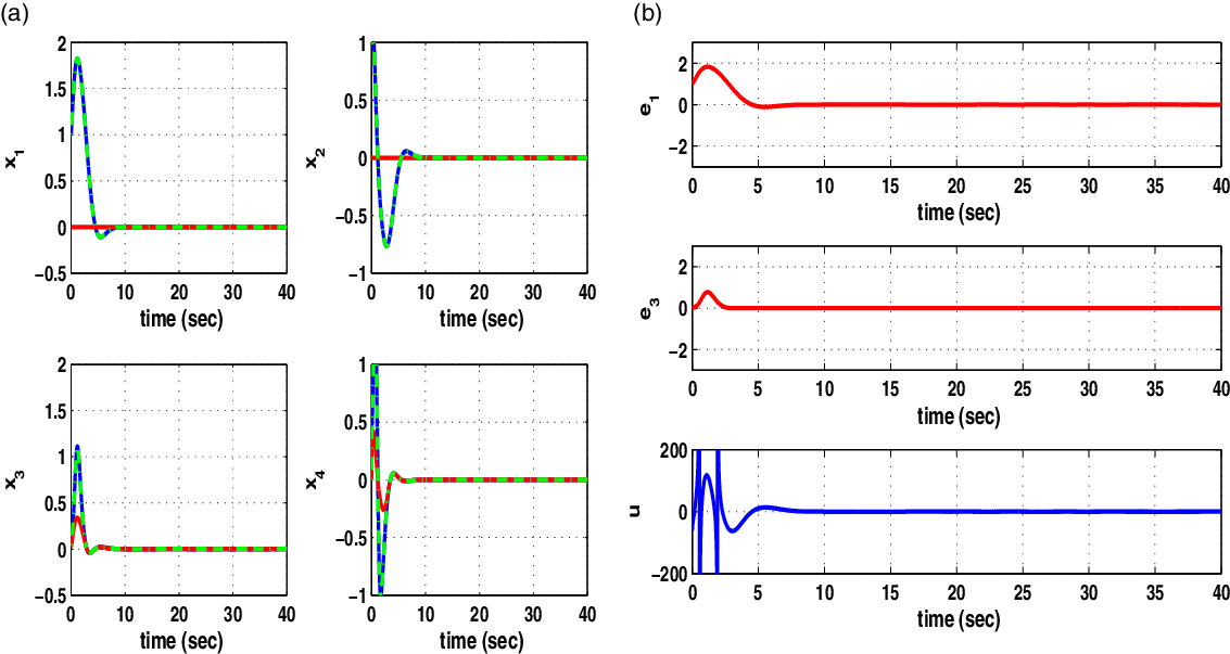
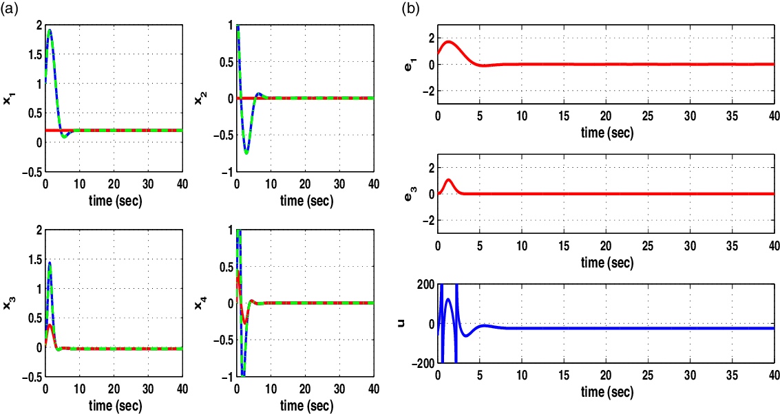
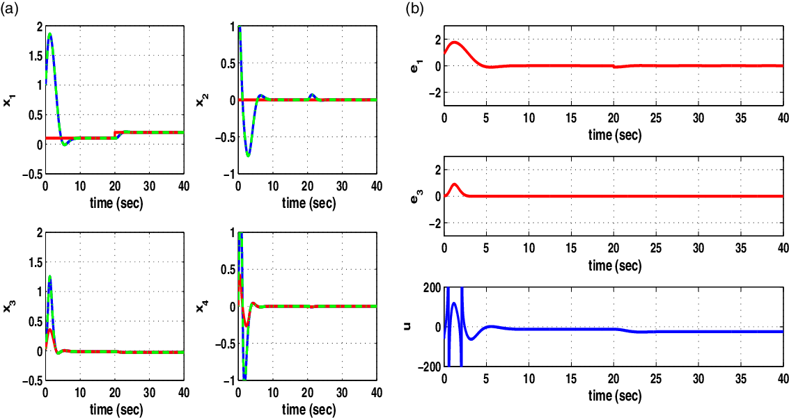
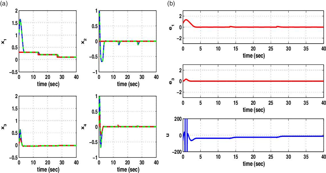
The tracking performance of the proposed nonlinear optimal (H-infinity) control method for PLI robots was tested through simulation experiments. Indicative values for the parameters of the model of the robotic mechanism are
 $l=0.5$
m,
 $d_1=0.5$
m,
 $g=10\,{\rm m/sec}^2$
,
 $m_1=63$
Kgr,
 $m_2=27$
Kgr,
 $h_1=0.18$
m, and
 $h_{20}=0.42$
m [Reference Dian, Chen, Hoang, Pu and Liu1]. The sampling period was
 $T_s=0.01$
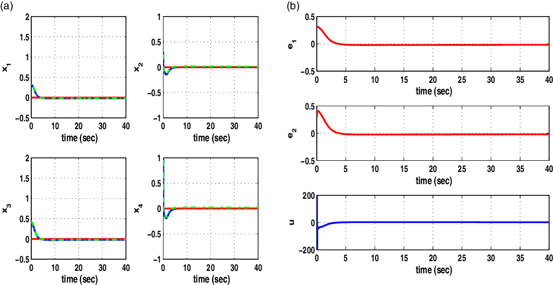
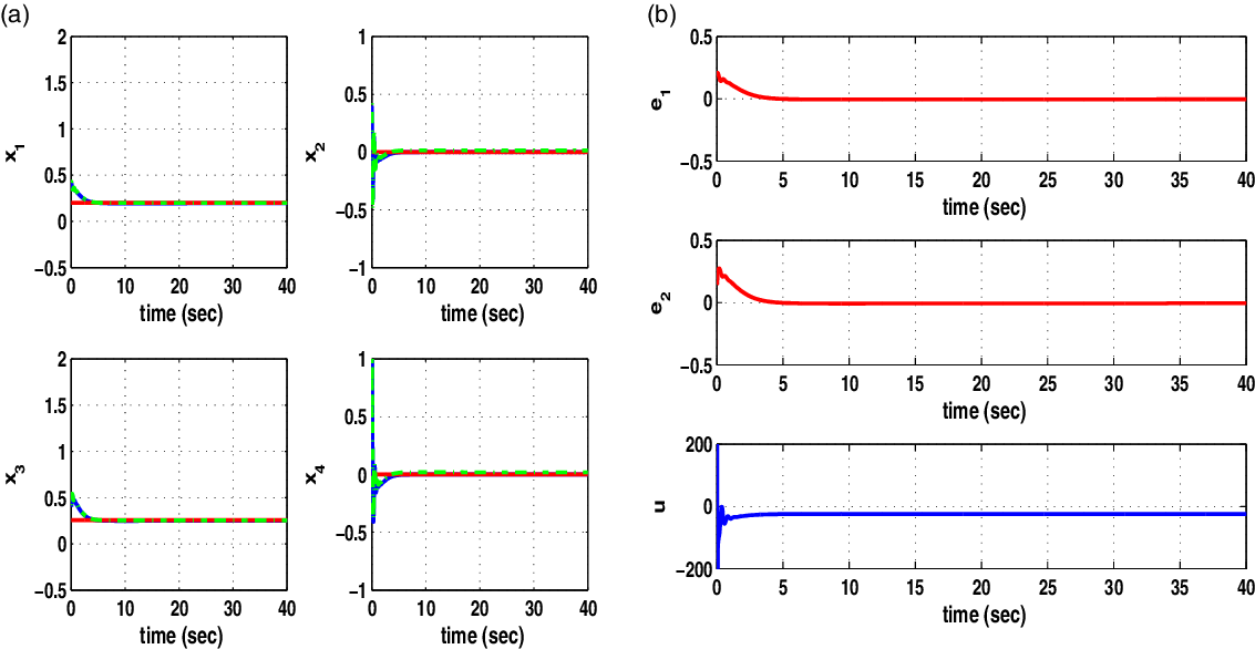
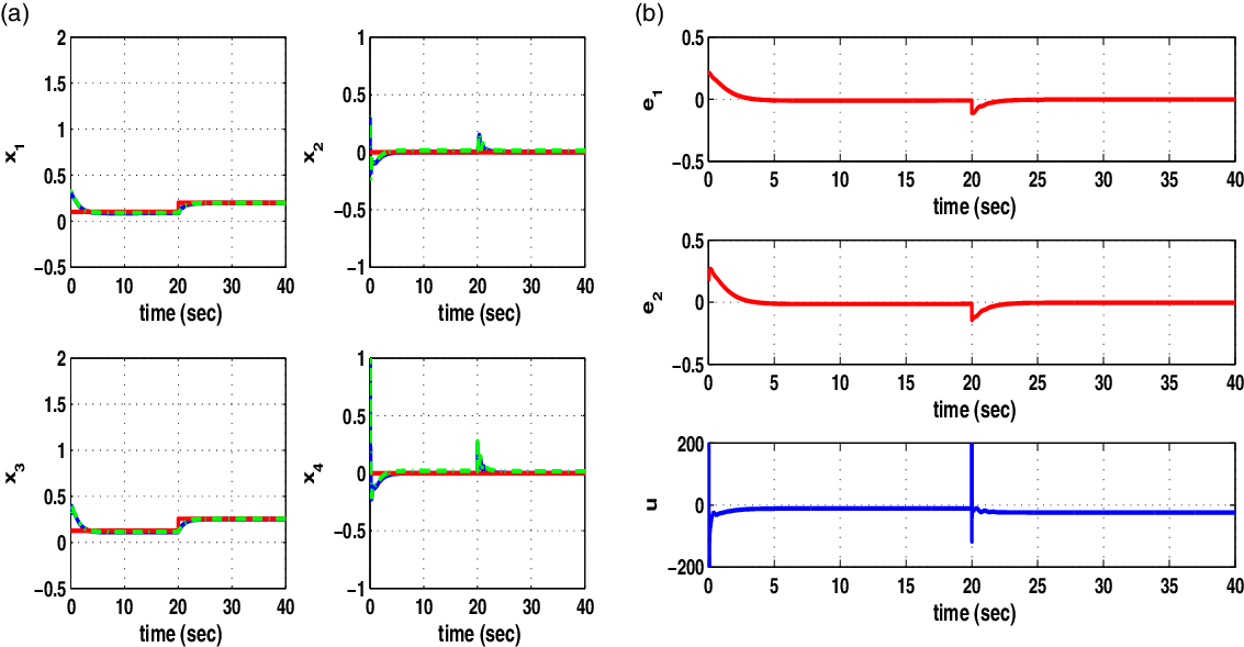
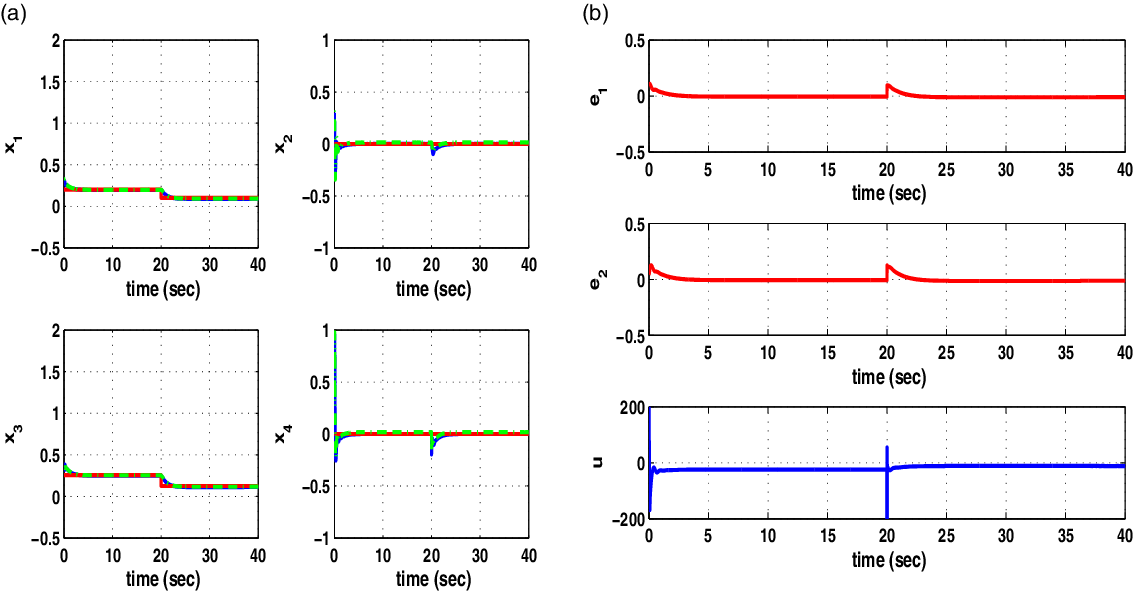
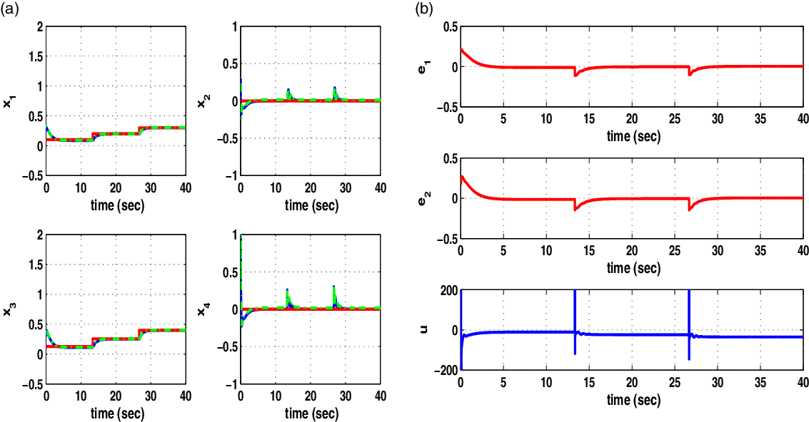
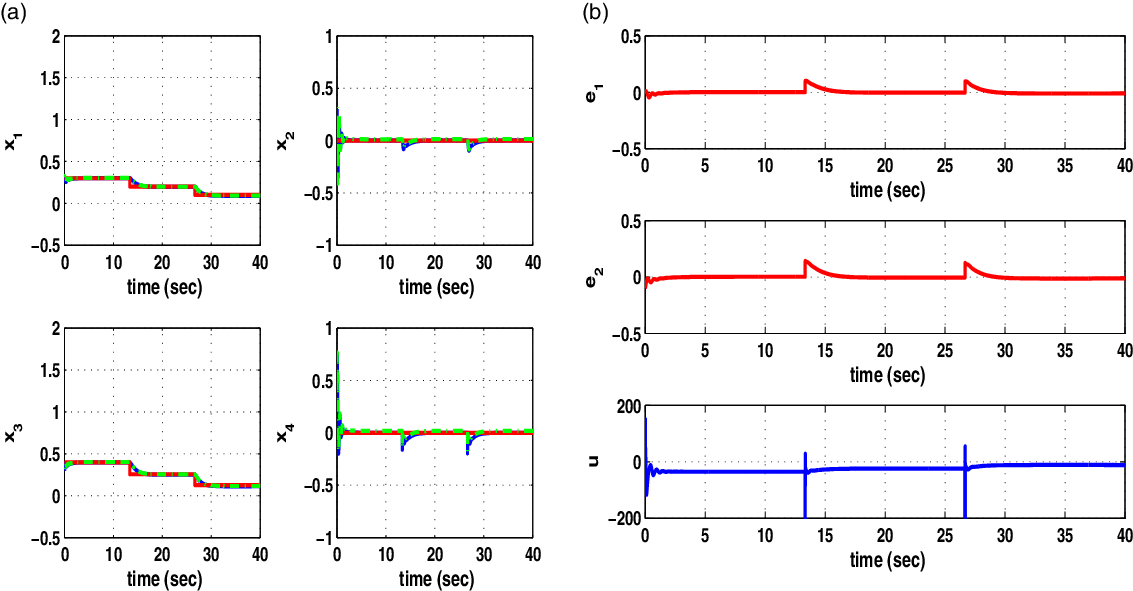
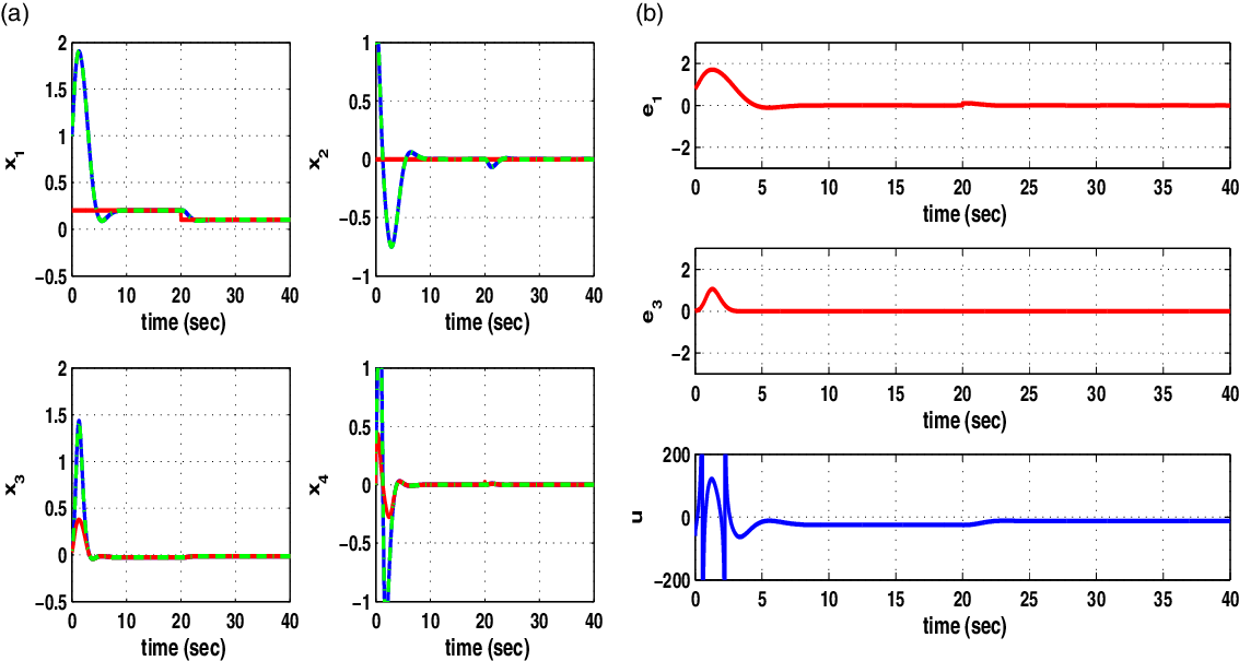
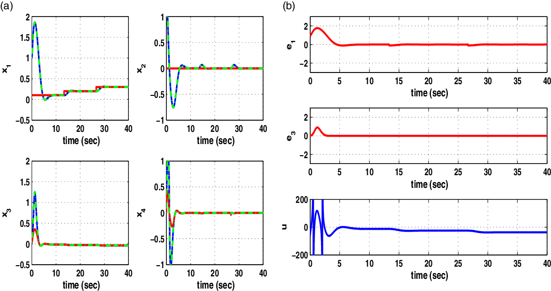
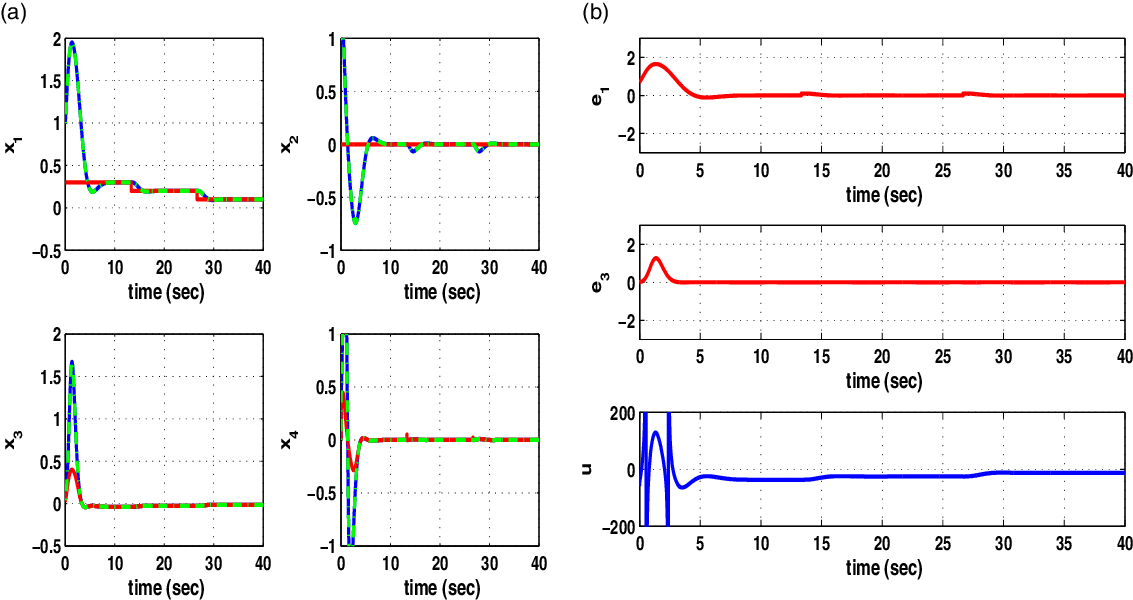
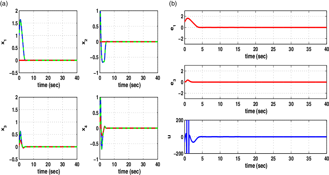
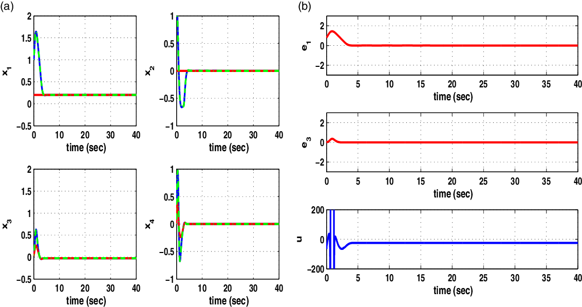
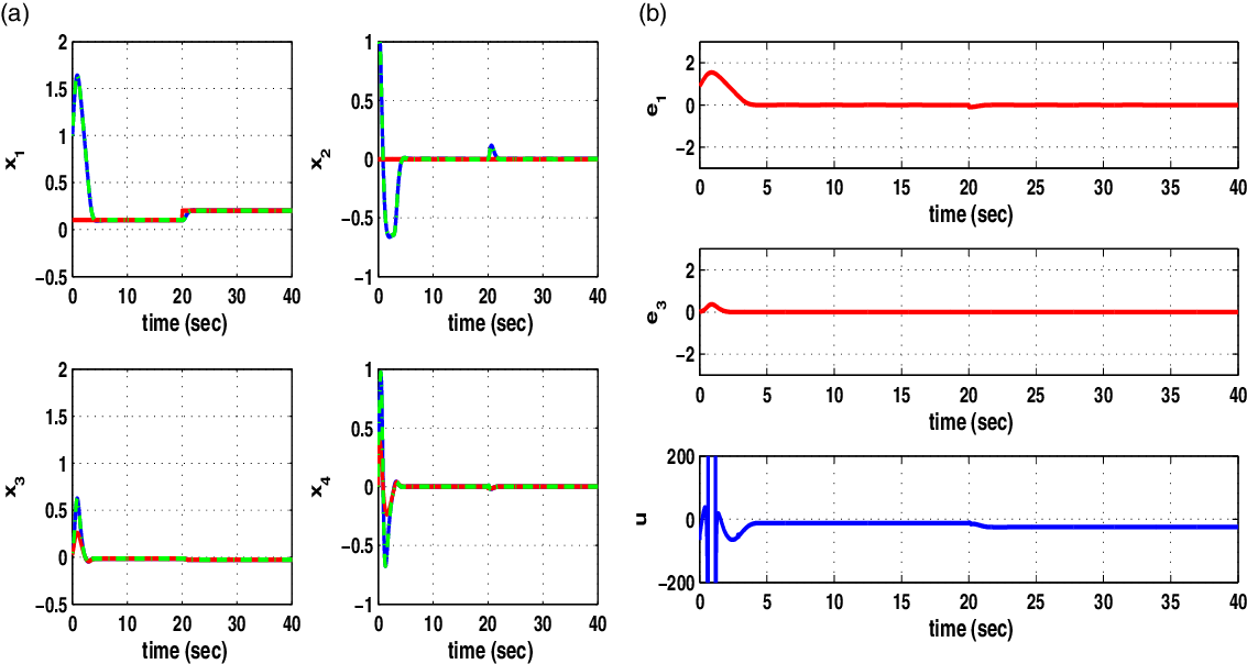
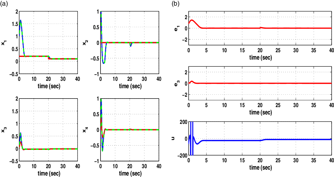
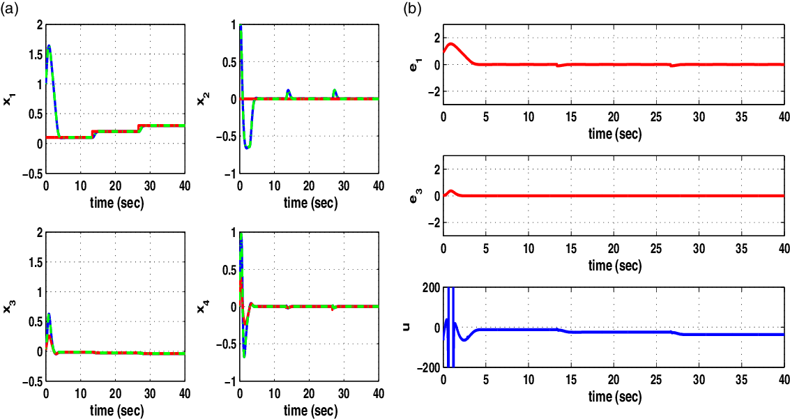
sec. The obtained results are given in Figs. 4, 5, 6, 7, 8, and 9. The state variables of the PLI robot are printed in blue color, the estimated state variables that were provided by the H-infinity Kalman filter are marked in green, while the related setpoints are plotted in red. The measurement units of angles
 $\theta_1$
and
 $\theta_2$
are in rad, while the measurement units of the angular velocities
 $\dot{\theta}_1$
and
 $\dot{\theta}_2$
are in rad/sec. The control input u is a torque measured in Ntm. It can be noticed that the tracking error for all state variables of the robotic mechanism has been eliminated, while the transient performance of the control loop was good. Actually, there were neither abrupt variations of the state variables nor excessive values of the control inputs. The transient performance of the control loop depends on the selection of values for parameters r,
 $\rho$
, and Q which appear in the algebraic Riccati equation given in Eq. (49). The smallest value of
 $\rho$
for which one can obtain a valid solution of the previously noted Riccati equation is the one that provides the control loop with maximum robustness.
Nonlinear optimal control of the power-line inspection robot when tracking setpoint 1 (a) state variables
 $x_i \ i=1,\cdots,4$
(blue lines), their estimated values (green lines) and the associated reference setpoints (red lines), (b) tracking errors
 $e_1$
(state variable
 $x_1$
) and
 $e_2$
(state variable
 $x_3$
) and control input u of the power-line inspection robot.

Nonlinear optimal control of the power-line inspection robot when tracking setpoint 2 (a) state variables
 $x_i \ i=1,\cdots,4$
(blue lines), their estimated values (green lines) and the associated reference setpoints (red lines), (b) tracking errors
 $e_1$
(state variable
 $x_1$
) and
 $e_2$
(state variable
 $x_3$
) and control input u of the power-line inspection robot.

Nonlinear optimal control of the power-line inspection robot when tracking setpoint 3 (a) state variables
 $x_i \ i=1,\cdots,4$
(blue lines), their estimated values (green lines) and the associated reference setpoints (red lines), (b) tracking errors
 $e_1$
(state variable
 $x_1$
) and
 $e_2$
(state variable
 $x_3$
) and control input u of the power-line inspection robot.

Nonlinear optimal control of the power-line inspection robot when tracking setpoint 4 (a) state variables
 $x_i \ i=1,\cdots,4$
(blue lines), their estimated values (green lines) and the associated reference setpoints (red lines), (b) tracking errors
 $e_1$
(state variable
 $x_1$
) and
 $e_2$
(state variable
 $x_3$
) and control input u of the power-line inspection robot.

Nonlinear optimal control of the PLI robot when tracking setpoint 5 (a) state variables
 $x_i \ i=1,\cdots,4$
(blue lines), their estimated values (green lines) and the associated reference setpoints (red lines), (b) tracking errors
 $e_1$
(state variable
 $x_1$
) and
 $e_2$
(state variable
 $x_3$
) and control input u of the PLI robot.

Nonlinear optimal control of the PLI robot when tracking setpoint 6 (a) state variables
 $x_i \ i=1,\cdots,4$
(blue lines), their estimated values (green lines) and the associated reference setpoints (red lines), (b) tracking errors
 $e_1$
(state variable
 $x_1$
) and
 $e_2$
(state variable
 $x_3$
) and control input u of the PLI robot.

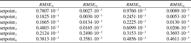
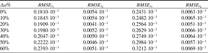
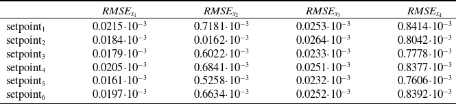
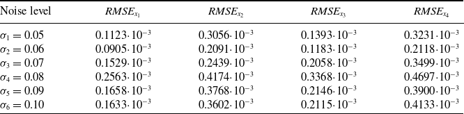
To elaborate on the tracking performance and on the robustness of the proposed nonlinear optimal control method for the PLI robot, the following tables are given: (i) Table I that provides information about the accuracy of tracking of the reference setpoints by the state variables of the PLI robot under an exact model, (ii) Table II that provides information about the robustness of the control method to parametric changes in the model of the PLI robot (change in drift term
 $f_2$
in the second row of the state-space model, up to 60%). Equivalent results, showing robustness of the control loop have been obtained for changes of the counter-weight mass
 $m_2$
of up to 20%. (iii) Table III which provides information about the precision in state variables’ estimation that is achieved by the H-infinity Kalman filter, (iv) Table IV which provides the tracking precision of the PLI robot under variable levels (variance) of sensors’ measurement noise.
Nonlinear optimal control RMSE for the PLI robot without disturbances.

Nonlinear optimal control RMSE for the PLI robot under disturbances.

Nonlinear optimal control RMSE for the estimation performed by the H-infinity KF.

Nonlinear optimal control RMSE for the PLI robot under variable noise levels.

Comparing to other nonlinear control methods for the model of the PLI robot, the proposed nonlinear optimal (H-infinity) control approach exhibits specific advantages (i) unlike global linearization-based control methods (such as Lie algebra-based control or differential flatness theory-based control), the article’s optimal control scheme does not need complicated state variables transformations (diffeomorphisms). Besides, in the article’s approach the control inputs are applied directly on the initial nonlinear state-space model of the PLI robot and not on its linearized equivalent description. Thus, the inverse transformations and the related singularity problems that may appear in global linearization-based control methods can be avoided. (ii) unlike popular approaches to optimal control met in industry, such as Model Predictive Control (MPC) and Nonlinear Model Predictive Control (NMPC) the stability and convergence of the article’s nonlinear optimal control scheme is assured. MPC is a linear control method and its use in the nonlinear dynamic model of the PLI robot will result into loss of stability. Besides, the convergence to an optimum for NMPC is dependent on initialization and parameter values selection and in general cannot be ascertained. (iii) unlike sliding-mode control and backstepping control, the application of the article’s control method does not require the state-space description of the system to be found in a specific form. In the case of sliding-mode control, one has to define the sliding surface however there is no systematic procedure about this unless the system is found in the input-output linearized (canonical) form. In the case of backstepping control the system has to be found in the backstepping integral (triangular) form. For the state-space model of the PLI robot, none of the above two conditions holds, therefore the use of the article’s nonlinear optimal control approach provides the only feasible solution, (iv) unlike PID control the article’s control method is of proven global stability, assures reliable functioning of the PLI robot at all changes of operating points and does not involve any heuristics in the selection of the controller’s gains, (v) unlike multiple models-based control, the article’s control method is computationally more efficient because it performs linearization only around one time-varying setpoint, and involves the solution of only one Riccati equation.
7.2. Results on flatness-based control of the PLI robot
Control of the PLI robot was also performed by applying differential flatness theory. The sampling period was
 $T_s=0.01$
sec. The input-output linearized state-space model of the PLI robot has been written in the canonical Brunvosky form. The design of a stabilzing feedback controller has been based on the pole-placement (eigenvalues assignment) technique) that was described in Section 5. The measurable state variable was the turn angle
 $x_1=\theta_1$
of the first joint of the robot. State estimation has been performed with the use of Kalman filtering. This filtering approach is also known as Derivative-free nonlinear Kalman filter (DKF). It consists of the Kalman filter’s recursion being applied to the linearized state-space description of the PLI robot and is followed by inverse transformations which provide finally the state estimates of the initial nonlinear model of the PLI robot [Reference Rigatos34]. The obtained results are shown in Figs. 10, 11, 12, 13, 14 and 15. It can be noticed that the differential flatness theory-based control method had also satisfactory performance. The tracking accuracy of the flatness-based control scheme was at the same order of the one achieved by the above-noted nonlinear optimal control scheme (this accuracy is dependent also on the selection of the feedback control gains).
Flatness-based control of the PLI robot when tracking setpoint 1: (a) state variables
 $x_i \ i=1,\cdots,4$
(blue lines), their estimated values (green lines) and the associated reference setpoints (red lines), (b) tracking errors
 $e_1$
(state variable
 $x_1$
) and
 $e_2$
(state variable
 $x_3$
) and control input u of the PLI robot.

Flatness-based control of the PLI robot when tracking setpoint 2: (a) state variables
 $x_i \ i=1,\cdots,4$
(blue lines), their estimated values (green lines) and the associated reference setpoints (red lines), (b) tracking errors
 $e_1$
(state variable
 $x_1$
) and
 $e_2$
(state variable
 $x_3$
) and control input u of the PLI robot.

Flatness-based control of the PLI robot when tracking setpoint 3: (a) state variables
 $x_i \ i=1,\cdots,4$
(blue lines), their estimated values (green lines) and the associated reference setpoints (red lines), (b) tracking errors
 $e_1$
(state variable
 $x_1$
) and
 $e_2$
(state variable
 $x_3$
) and control input u of the PLI robot.

Flatness-based control of the PLI robot when tracking setpoint 4: (a) state variables
 $x_i \ i=1,\cdots,4$
(blue lines), their estimated values (green lines) and the associated reference setpoints (red lines), (b) tracking errors
 $e_1$
(state variable
 $x_1$
) and
 $e_2$
(state variable
 $x_3$
) and control input u of the PLI robot.

Flatness-based control of the PLI robot when tracking setpoint 5: (a) state variables
 $x_i \ i=1,\cdots,4$
(blue lines), their estimated values (green lines) and the associated reference setpoints (red lines), (b) tracking errors
 $e_1$
(state variable
 $x_1$
) and
 $e_2$
(state variable
 $x_3$
) and control input u of the PLI robot.

Flatness-based control of the PLI robot when tracking setpoint 6: (a) state variables
 $x_i \ i=1,\cdots,4$
(blue lines), their estimated values (green lines) and the associated reference setpoints (red lines), (b) tracking errors
 $e_1$
(state variable
 $x_1$
) and
 $e_2$
(state variable
 $x_3$
) and control input u of the PLI robot.

7.3. Results on sliding-mode control of the PLI robot
Control of the PLI robot was also performed by applying sliding-mode control. The sampling period was again
 $T_s=0.01$
sec. The input-output linearized state-space model of the PLI robot has been written in the canonical Brunvosky form. The design of the sliding-mode control has been based on the technique that was described in Section 6. The measurable state variable was the turn angle
 $x_1=\theta_1$
of the first joint of the robot. State estimation has been performed with the use of Kalman filtering as in the case of flatness-based control [Reference Rigatos34]. The obtained results are shown in Figs. 16, 17, 18, 19, 20 and 21. It can be noticed that sliding-mode control had also satisfactory performance. The tracking accuracy of the sliding-mode control scheme was at the same order of the one achieved by the above-noted nonlinear optimal control scheme. To limit the variations of the control inputs and to avoid the appearance of chattering in the control signal the switching control term based on a sign function of the sliding surface s was substituted by a saturation function.
Sliding-mode control of the PLI robot when tracking setpoint 1: (a) state variables
 $x_i \ i=1,\cdots,4$
(blue lines), their estimated values (green lines) and the associated reference setpoints (red lines), (b) tracking errors
 $e_1$
(state variable
 $x_1$
) and
 $e_2$
(state variable
 $x_3$
) and control input u of the PLI robot.

Sliding-mode control of the PLI robot when tracking setpoint 2: (a) state variables
 $x_i \ i=1,\cdots,4$
(blue lines), their estimated values (green lines) and the associated reference setpoints (red lines), (b) tracking errors
 $e_1$
(state variable
 $x_1$
) and
 $e_2$
(state variable
 $x_3$
) and control input u of the PLI robot.

Sliding-mode control of the PLI robot when tracking setpoint 3: (a) state variables
 $x_i \ i=1,\cdots,4$
(blue lines), their estimated values (green lines) and the associated reference setpoints (red lines), (b) tracking errors
 $e_1$
(state variable
 $x_1$
) and
 $e_2$
(state variable
 $x_3$
) and control input u of the PLI robot.

Sliding-mode control of the PLI robot when tracking setpoint 4: (a) state variables
 $x_i \ i=1,\cdots,4$
(blue lines), their estimated values (green lines) and the associated reference setpoints (red lines) (b) tracking errors
 $e_1$
(state variable
 $x_1$
) and
 $e_2$
(state variable
 $x_3$
) and control input u of the PLI robot.

Sliding-mode control of the PLI robot when tracking setpoint 5: (a) state variables
 $x_i \ i=1,\cdots,4$
(blue lines), their estimated values (green lines) and the associated reference setpoints (red lines) (b) tracking errors
 $e_1$
(state variable
 $x_1$
) and
 $e_2$
(state variable
 $x_3$
) and control input u of the power-line inspection robot.

Sliding-mode control of the power-line inspection robot when tracking setpoint 6: (a) state variables
 $x_i \ i=1,\cdots,4$
(blue lines), their estimated values (green lines) and the associated reference setpoints (red lines), (b) tracking errors
 $e_1$
(state variable
 $x_1$
) and
 $e_2$
(state variable
 $x_3$
) and control input u of the power-line inspection robot.

Remark 2: Although NMPC is a popular approach for implementing optimal control in industrial and robotic systems, the method’s performance is not always proven, while the performance of its iterative search for an optimum is dependent on ad-hoc selection of the values of specific parameters. On the other side, the application of the back-stepping control method as presented in [Reference Dian, Chen, Hoang, Pu and Liu1] requires some transformations and simplifications of the state-space model of the power-line inspection robot, so as to obtain finally a description in the back-stepping integral (strict-feedback) form. Additionally, the application of flatness-based control requires to prove first the differential flatness properties of the dynamic model of the power-lines inspection robot. This is enabled only after some changes and simplifications are performed in the initial nonlinear model of the robot, as described in Section 5. Equivalently, to apply sliding-mode control to the dynamic model of PLI robots, the selection of sliding surfaces is in general an intuitive procedure. Only after transformation in the state-space form of Section 5.1 there exists a well-defined procedure for defining sliding surfaces and for implementing sliding-mode control.
8. Conclusions
A nonlinear optimal (H-infinity) control method has been developed for the dynamic model of a power-lines inspection robot. Control and stabilization of this type of robot is a nontrivial problem because of the nonlinear dynamics of the robotic mechanism, as well as because of underactuation. Actually, the considered robotic system has two degrees of freedom while receiving only one control input. To achieve a solution for this control problem, the dynamic model of the PLI robot has undergone first approximate linearization around a time-varying operating point which was updated at each time-step of the control method. The linearization process relied on first-order Taylor series expansion and on the computation of the related Jacobian matrices.
For the approximately linearized model of the PLI robot an H-infinity feedback controller was designed. To compute the controller’s gains an algebraic Riccati equation was repetitively solved at each iteration of the control algorithm. The global stability properties of the control scheme were proven through Lyapunov analysis. The proposed nonlinear optimal (H-infinity) control method retains the advantages of linear optimal control, that is fast and accurate tracking of reference setpoints under moderate variations of the control inputs. The method has been also compared against flatness-based control and sliding-mode control. The benefit from the application of the nonlinear optimal control method is in assuring the precise functioning of the PLI robot under minimal dissipation of energy by its actuators. Such a type of robots can release the power grid’s maintenance personnel from dangerous tasks related with the inspection of overhead cables of the power transmission and distribution system.