1 Introduction
The Apollonian (or curvilinear Sierpinski) gasket is one of the most well-known and widely studied fractals. Beyond its prevalence in fractal geometry and dynamical systems, it has important connections to several branches of mathematics such as number theory, hyperbolic geometry and Fuchsian groups, and group theory, see, for example, the surveys [Reference Oh16, Reference Pollicott17].
The gasket is the residual set of the standard Apollonian circle packing. Starting with three mutually tangent circles with no triple tangencies, we let
$T_1$
 be the residual curvilinear triangle. A famous theorem of Apollonius of Perga asserts that there are two circles (known as the inner and outer Soddy circles) which are tangent to the three original circles. The inner Soddy circle lies in the interstice between the mutually tangent original circles and gives rise to three new residual curvilinear triangles inside
$T_1$
 whose union is denoted by
$T_2$
 . Continuing iteratively, three new inner Soddy circles can be found inside
$T_2$
 giving rise to nine residual curvilinear triangles inside
$T_2$
 and so on. The set
$\bigcap _{n=1}^\infty T_n$
 is called an Apollonian gasket. Notice that, since the Hausdorff dimension is a conformal invariant (as it is bi-Lipschitz invariant), the Hausdorff dimension of the residual set (the gasket) is independent of the size of the first three circles.
The dimension theory of the Apollonian gasket has attracted considerable attention from various researchers since the 1960s [Reference Bai and Finch1, Reference Boyd2, Reference Chousionis, Leykekhman, Urbański and Wendt5, Reference Hirst8, Reference McMullen15, Reference Thomas and Dhar18, Reference Vytnova and Wormell21]. However, several of these contributions were not rigorously justified and until 2024, the best rigorous estimates for the Hausdorff dimension of the Apollonian gasket were due to Boyd [Reference Boyd2] from the early 1970s. Recently, Vytnova and Wormell [Reference Vytnova and Wormell21] obtained rigorous Hausdorff dimension estimates with precision of 128 digits. In [Reference Chousionis, Leykekhman, Urbański and Wendt5], we introduced a general framework for rigorously estimating the Hausdorff dimension of a wide class of conformal fractals—specifically, the limit sets of maximal conformal graph-directed Markov systems—including the Apollonian gasket and its various subsystems. Although our approach yields estimates that are considerably less precise than those in [Reference Vytnova and Wormell21], it is very fast and offers remarkable flexibility for estimating Hausdorff dimensions of subsystems with four to five digits of precision. As will be clear from the following presentation, this feature is absolutely essential for the proof of Theorem 1.1.
It is well known that the Apollonian gasket can be obtained as a limit set of an iterated function system (IFS) consisting of three conformal maps. However, these generators are not contracting (only non-expansive), and this is a serious obstacle in analyzing the dimensional and geometric properties of the Apollonian gasket. The recent advances [Reference Chousionis, Leykekhman, Urbański and Wendt5, Reference Vytnova and Wormell21] rely on the fact that the Apollonian gasket can also be viewed as the limit set of an infinitely generated conformal iterated function system (CIFS) consisting of uniformly contracting maps. More precisely, there exists a CIFS
$\mathcal {A}$
 (see the beginning of §3) whose limit set
$J_{\mathcal {A}}$
 is equal to the Apollonian gasket minus the countable set of its cusp points. This was realized by Mauldin and Urbański in [Reference Mauldin and Urbański13], and it was used to verify that the Apollonian gasket has positive and finite h-Hausdorff measure and infinite h-packing measure, where
$h=\dim _{H}(J_{\mathcal {A}})=1.30568\cdots $
 is the Hausdorff dimension of the Apollonian gasket.
We contribute to the dimension theory of the Apollonian gasket by determining its (Hausdorff) dimension spectrum. We first recall how the dimension spectrum of IFSs is defined. Let
$X \subset \mathbb R^n$
 be a compact set and let
$\mathcal {S}=\{\phi _i:X \rightarrow X\}_{i \in I}$
 be a countable collection of uniformly contracting maps. If
$A \subset I$
 , we denote the corresponding subsystem of
$\mathcal {S}$
 by
$\mathcal {S}_A=\{\phi _i:X \rightarrow X\}_{i \in A}$
 and we denote its limit set by
$J_A$
 . The dimension spectrum of
$\mathcal {S}$
 is the set of all possible values of the Hausdorff dimension of the subsystems of
$\mathcal {S}$
 , that is,

If
$\mathcal {S}$
 consists of finitely many maps, then
$DS(\mathcal {S})$
 is a finite set. However, in the case when
$\mathcal {S}$
 is infinite, the structure of the dimension spectrum becomes significantly richer and more intricate.
The dimension spectrum was first studied by Mauldin and Urbański in [Reference Mauldin and Urbański12] where they showed that if
$\mathcal {S}$
 is a CIFS, then
$[0,\theta ) \subset DS(\mathcal {S})$
 where
$\theta $
 is the finiteness parameter of the system, see (2.5). Naturally, one is interested in systems whose dimension spectrum is an interval; that is, systems which satisfy
$DS(\mathcal {S})=[0, \dim _{H}(J_{\mathcal {S}})]$
 . In that case, we say that
$\mathcal {S}$
 has full dimension spectrum. In a significant contribution, Kesseböhmer and Zhu [Reference Kesseböhmer and Zhu10] proved that the dimension spectrum of the CIFS resulting from the real continued fractions algorithm is full; thus, resolving the so-called Texan conjecture. The result in [Reference Kesseböhmer and Zhu10] can be restated as follows; given any
$t \in [0,1]$
 , there exists
$E_t \subset {\mathbb {N}}$
 such that the set of irrational numbers whose continued fraction expansion only contains digits from
$E_t$
 has Hausdorff dimension t.
More recently, the first three authors introduced a rigorous computational approach in [Reference Chousionis, Leykekhman and Urbański3, Reference Chousionis, Leykekhman and Urbański4], drawing partial inspiration from the methods developed in [Reference Kesseböhmer and Zhu10], to study the dimension spectrum of various conformal fractals associated with continued fractions. In particular, [Reference Chousionis, Leykekhman and Urbański4] established that the CIFSs arising from real continued fractions—when restricted to alphabets such as the set of prime numbers, perfect squares, or any arithmetic progression—possess full dimension spectrum. Additionally, [Reference Chousionis, Leykekhman and Urbański3] demonstrated that the standard CIFS derived from complex continued fractions also has full dimension spectrum. We note that the dimension spectrum of infinite IFSs can be very different than an interval as it may have many non-degenerate connected components and connected components being singletons. Such examples can be found in [Reference Chousionis, Leykekhman and Urbański4, Reference Das and Simmons7, Reference Kesseböhmer and Zhu10]. However, it was proved in [Reference Chousionis, Leykekhman and Urbański3] that in the case of CIFSs, the dimension spectrum is always compact and perfect. Interestingly, this is not always the case for affine IFSs, see [Reference Jurga9].
In this paper, we combine methods from [Reference Chousionis, Leykekhman and Urbański3] together with our recent computational approach from [Reference Chousionis, Leykekhman, Urbański and Wendt5] to prove the following theorem.
Theorem 1.1. The dimension spectrum of the infinitely generated Apollonian gasket is full, that is,

We now discuss briefly the proof of Theorem 1.1. Our starting point is [Reference Chousionis, Leykekhman and Urbański3, Proposition 6.17]. Given any CIFS
$\mathcal {S}=\{\phi _i:X \to X\}_{i \in I}$
 , a well-ordering
$\prec $
 on the alphabet I is called natural (with respect to
$\mathcal {S}$
 ) if

If
$I=\{i_n\}_{n \in {\mathbb {N}}}$
 is an enumeration respecting
$\prec $
 , then we denote the m-initial segments by
$I(m)=\{i_1,\ldots ,i_m\}.$
 According to [Reference Chousionis, Leykekhman and Urbański3, Proposition 6.17], if K is a distortion bound for
$\mathcal {S}$
 (see (2.1)) and there exist
$t_1 \leq t_2 \leq \dim _{H}(J_{\mathcal {S}})$
 and
$d \in {\mathbb {N}}$
 such that
-
(1) $\dim J_{I_d} \leq t_1$
 ,
-
(2) $\sum _{n \geq k+1} \| \phi _{i_n}'\|_\infty ^{t_2} \geq K^{2t_2} \|\phi _{i_k}'\|^{t_2}_\infty $
for all
$k \geq d+1$
,


then
$[t_1,t_2] \subset DS(\mathcal {S})$
 .
If one wants to apply the previous scheme to find intervals inside the spectrum of the Apollonian system
$\mathcal {A}$
 , first one has to find a computationally friendly distortion constant
$K_{\mathcal {A}}$
 . We deal with this problem in §3 and we prove in Proposition 3.5 that

As far as we know, this is the first time that such a distortion constant has been obtained. We consider that our distortion bound is of independent interest and likely will be useful for other related problems. Moreover, motivated by our bound, one can naturally ask what is the best distortion constant for the Apollonian system
$\mathcal {A}$
 . We note that although the proof of Proposition 3.5 is quite technical, it only uses elementary tools.
With a reasonably sized distortion constant at hand, we use an iterative bootstrapping argument in §4, similar to that from [Reference Chousionis, Leykekhman and Urbański3], to identify a chain of
$18$
 overlapping intervals contained in
$DS(\mathcal {A})$
 and containing
$[1/2, \dim_{H}(J_{\mathcal{A}})]$
 . This is enough because by [Reference Mauldin and Urbański12, Reference Mauldin and Urbański13], we know that
$[0,1/2) \subset DS (\mathcal {A})$
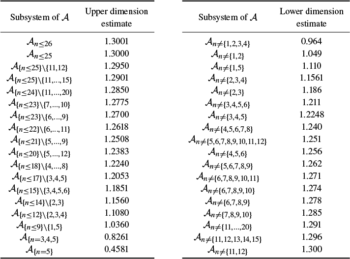
 . Here is exactly where our flexible approach from [Reference Chousionis, Leykekhman, Urbański and Wendt5] comes in very handy. Using the method developed in [Reference Chousionis, Leykekhman, Urbański and Wendt5], we are able to rigorously estimate upper and lower bounds for the Hausdorff dimension of various Apollonian subsystems (see Table 2) with sufficient accuracy for our bootstrapping argument to work. All
$18$
 steps are summarized in Table 1. We would like to point out that obtaining a good upper bound for the distortion constant of
$\mathcal {A}$
 is essential; it allows us to take the first crucial step which produces a small interval in the spectrum that includes
$\dim _{H} (J_{\mathcal {A}})$
 .
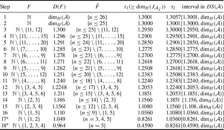
Summary of how Corollary 4.3 is applied in each step of the iteration (
$t_1$
 ,
$t_2$
 , F, and
$\tilde {F}$
 are as in that corollary). In particular,
$t_1$
 is an upper bound of
$\dim _{H} (J_{\mathcal {A}_{\tilde {F}}})$
 and
$D(F)$
 is a lower bound of
$\dim _{H}(J_{\mathcal {A}_F})$
 . To be able to apply Corollary 4.3, we need to know that
$t_2 \leq D(F)$
 . In steps 1–16,
$K_F=K_{\mathcal {A}} =5.900319$
 . In steps 17 and 18,
$K_F=K_{\mathcal {A}_{n>2}}=4.3655$
 , see Proposition 3.5.

Table 1 Long description
A table with 18 rows and 7 columns detailing iterative mathematical steps.
Columns are labeled:
1. Step
2. F
3. D(F)
4. F-tilde
5. t sub 1 (greater than or equal to dim sub H (J sub A sub F-tilde))
6. t sub 2
7. interval in D S (A)
Key data points include:
* Step 1: F is the set of natural numbers N; D(F) is dim sub H (A); F-tilde is {n <= 26}; t sub 1 is 1.3001; t sub 2 is 1.3057; interval is [1.3001, dim sub H (A)].
* Step 5: F is N minus {11, ..., 20}; D(F) is 1.291; F-tilde is {n <= 24} minus {11, ..., 20}; t sub 1 is 1.2850; t sub 2 is 1.2901; interval is [1.2850, dim sub H (A)].
* Step 10: F is N minus {5, ..., 12}; D(F) is 1.251; F-tilde is {n <= 20} minus {5, ..., 12}; t sub 1 is 1.2383; t sub 2 is 1.2508; interval is [1.2383, dim sub H (A)].
* Step 15: F is N minus {2, 3, 4}; D(F) is 1.1561; F-tilde is {n <= 12} minus {2, 3, 4}; t sub 1 is 1.1080; t sub 2 is 1.1560; interval is [1.108, dim sub H (A)].
* Step 18*: F is N minus {1, 2, 3, 4}; D(F) is 0.964; F-tilde is {n = 5}; t sub 1 is 0.4590; t sub 2 is 0.8261; interval is [0.4590, dim sub H (A)].
As the steps progress, the values for D(F), t sub 1, and t sub 2 generally decrease, narrowing the calculated intervals.
The paper is structured as follows. Section 2 introduces the necessary background for CIFSs and their thermodynamic formalism. In §3, which is the main technical part of our paper, we obtain an estimate for the distortion constant of the Apollonian system. Finally, in §4, we prove Theorem 1.1.
2 Preliminaries
We start by introducing some necessary background on CIFSs. Let X be a compact metric space. An IFS on X is a countable family
$\mathcal {S}=\{\phi _{i}:X \to X\}_{i \in I}$
 of injective contractions whose Lipschitz constant is less than s for some
$s \in (0,1)$
 .
If
$\omega \in I^*:=\bigcup _{n=0}^\infty I^n$
 , we denote by
$|\omega |$
 the unique integer
$n \geq 0$
 such that
$\omega \in I^n$
 , and we call
$|\omega |$
 the length of
$\omega $
 . If
$\omega \in I^{\mathbb {N}}$
 or
$|\omega |>n$
 , we let
$ \omega |_n:=\omega _1\ldots \omega _n\in I^n$
 . Given
$\omega \in I^{{\mathbb {N}}}$
 , we denote
$\phi _{\omega |_n}=\phi _{\omega _1} \circ \cdots \phi _{\omega _n}.$
 Note that the non-empty compact sets
$\{\phi _{\omega |_n}(X)\}_{n=1}^\infty $
 form a decreasing sequence with non-empty intersection. Since
$\text {diam}(\phi _{\omega |_n}(X)) \le s^n\text {diam}(X), \text { for all } n \in {\mathbb {N}},$
 we can define the coding map
$\pi :I^{\mathbb {N}}\to X$
 given by

The set
$ J=J_{\mathcal {S}}:=\pi (I^{{\mathbb {N}}}) $
 is called the limit set (or attractor) of the IFS
$\mathcal {S}$
 .
We are interested in CIFS in the complex plane.
Definition 2.1. Let
$X \subset \mathbb C$
 be compact and connected. An IFS
$\mathcal {S}=\{\phi _i:X \to X\}_{i \in I}$
 is called conformal if the following conditions are satisfied.
-
(1) There exists an open and connected set $W \supset X$
such that the maps
$\phi _i, i \in I,$
extend to a
$C^1$
conformal diffeomorphism of W into W. -
(2) (Open set condition or OSC). For all $i,j\in I$
,
$i\ne j$
, $$ \begin{align*} \phi_i(\operatorname{\mathrm{Int}}(X)) \cap \phi_j(\operatorname{\mathrm{Int}}(X))= \emptyset. \end{align*} $$


It follows by [Reference Mauldin and Urbański14, Reference Kotus and Urbański11] that CIFSs in the complex plane satisfy the bounded distortion property (BDP): there exists some constant
$K \geq 1$
 , depending only on
$\mathcal {S}$
 , such that

for every
$\omega \in I^*$
 and every pair of points
$p,q\in X$
 . If K is as in (2.1), it is called a distortion constant of
$\mathcal {S}$
 . Given
$\omega \in I^\ast$
 , we let

The Leibniz rule and (2.1) imply that if
$\omega \in I^\ast $
 and
$\omega =\tau \upsilon $
 for some
$\tau , \upsilon \in I^\ast $
 , then

We now briefly recall some facts from the thermodynamic formalism of CIFSs, see e.g. [Reference Mauldin and Urbański12, Reference Mauldin and Urbański14, Reference Urbański, Roy and Munday19] for more information. Let
$\mathcal {S}=\{\phi _i\}_{i\in I}$
 be a CIFS. For
$t\ge 0$
 and
$n \in {\mathbb {N}}$
 , let

Since, by (2.2),

the sequence
$\{\log Z_n(t)\}_{n=1}^\infty $
 is subadditive. Thus, the limit

exists and it is called the topological pressure of the system
$\mathcal {S}$
 evaluated at the parameter t. We record that
$t \mapsto P(t)$
 is a decreasing function on
$[0,+\infty )$
 with
$\lim _{t \rightarrow +\infty } P(t)= -\infty $
 . Moreover, P is convex and continuous on
$\overline {\{t \geq 0: P(t)<\infty \}}$
 , see e.g. [Reference Urbański, Roy and Munday19, Proposition 19.4.6]. We also let

It is well known, see e.g. [Reference Urbański, Roy and Munday19, Proposition 19.4.4], that

The parameter
$h(\mathcal {S})$
 is known as Bowen’s parameter and it coincides with the Hausdorff dimension of the limit set
$J_{\mathcal {S}}$
 .
Theorem 2.2. [Reference Mauldin and Urbański12]
If
$\mathcal {S}$
 is a CIFS, then

We note that Theorem 2.2 has been generalized to various settings, see e.g. [Reference Mauldin and Urbański14, Theorem 4.2.13] or [Reference Chousionis, Tyson and Urbański6, Theorem 7.19].
3 Effective bounds of the Apollonian gasket’s distortion
From now on, we focus on the Apollonian gasket. We first introduce an infinite CIFS whose limit set coincides with the Apollonian gasket minus the countable set of its cusp points.
We consider the angles

and the maps

where
$R_\theta $
 is the standard complex rotation by the angle
$\theta $
 . Let
$\mathbb D=B(0,1)$
 be the unit disk in the complex plane and let
$I=\{1,2, \ldots , 6 \} \times {\mathbb {N}}$
 . The Apollonian IFS is then defined as

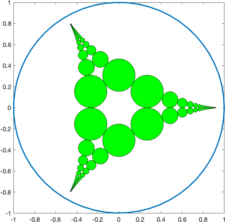
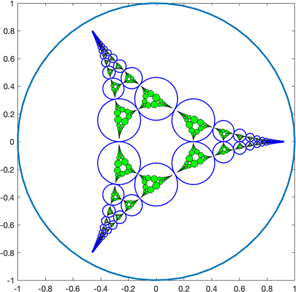
The first two iterations of the maps are displayed in Figures 1 and 2.
One iteration (colour online).

Figure 1 Long description
A mathematical plot on a Cartesian grid with x and y axes ranging from negative 1 to 1. A thick blue boundary circle is centered at 0, 0 with a radius of 1. Inside this boundary is a fractal packing of solid green circles with black outlines. At the very center of the plot is a small white circular void. Surrounding this void are six large green circles arranged in a hexagonal ring. From this central ring, the green circles branch out in three directions toward the top-left, bottom-left, and middle-right, forming a triangular or star-like symmetry. In each of the three branches, the circles decrease in size recursively as they approach the outer blue boundary. The largest circles are near the center, and they become progressively smaller, appearing as tiny dots as they converge toward three specific points on the perimeter of the fractal structure.
Two iterations (colour online).

Figure 2 Long description
The plot is set on a square grid with X and Y axes ranging from minus 1 to 1. A large blue circle with a radius of 1 serves as the outer boundary. Inside this boundary is a fractal structure composed of blue-outlined circles containing smaller green-filled circles. The overall shape of the fractal is a three-pointed star or triangular configuration. At the center of the plot is an empty triangular space surrounded by three large blue circles. Within each of these blue circles, smaller green circles are arranged in a recursive triangular pattern. This pattern repeats and scales down as it moves outward toward three main vertices located at approximately (0.9, 0), (minus 0.45, 0.8), and (minus 0.45, minus 0.8). As the circles approach these vertices, they become increasingly dense and microscopic, creating a tapering effect that defines the three points of the fractal star.
It was proved in [Reference Mauldin and Urbański13] that
$\mathcal {A}$
 is a CIFS; it satisfies the conditions from Definition 2.1. We also note that the set W (as it appears in Definition 2.1) it can be taken to be
$B(0,1+\sqrt {3})$
 , that is,

see [Reference Chousionis, Leykekhman, Urbański and Wendt5, Proposition 6.7]. We also need to consider certain subsystems of
$\mathcal {A}$
 . If
$F\subset {\mathbb {N}}$
 , we let

where

From now on, we let
$\unicode{x3bb} :=\sqrt {3}$
 . Our proof depends on effective bounds of the distortion constant of
$\mathcal {A}$
 . These estimates require us to find the radii of the disks
$\phi _{k,n} (\mathbb D)$
 for
$n=1,2,3$
 .
Proposition 3.1. Let
$k=1,\ldots ,6$
 :
-
(1) $\text {radius}\,\phi _{k,1}(\mathbb D)=({2 \unicode{x3bb} -3})/{3}$
; -
(2) $\text {radius}\, \phi _{k,2}(\mathbb D)=({14\unicode{x3bb} -15})/{121}$
; -
(3) $\text {radius} \, \phi _{k,3}(\mathbb D)=({26\unicode{x3bb} - 21})/{529}$
.


Moreover, the centers of the disks
$\phi _{k,1}(\mathbb D), k=1,\ldots ,6,$
 lie on
$\partial B(0, ({4 \unicode{x3bb} -6})/{3})$
 .
Proof. We first prove item (1). Let
$k=1,\ldots ,6$
 . The matrix representation of the map
$F_k:=f \circ R_{\theta _k} \circ f$
 is given by

thus,

If k is even (that is,
$\theta _k=2\pi /3$
 ), we set
$F_k:=F_e$
 and if k is odd (that is,
$\theta =-2\pi /3$
 ), we set
$F_k:=F_o$
 .
We first assume that k is even. Picking three points on the unit circle
$z_1=1$
 ,
$z_2= e^{2\pi /3}$
 , and
$z_3= e^{-2\pi /3}$
 , we have

Thus, we need to compute the center and radius of the circle passing through

This is equivalent to solving the
$3\times 3$
 linear system
$Ax=b$
 , where

Inverting A, we obtain

and, consequently,

Thus,

Since
$F_o(z)=\overline {F_e(\bar {z})}$
 , we deduce that

Recalling that
$\phi _{k,1}=R_{\theta _k'} \circ f \circ R_{\theta _k} \circ f$
 , we deduce item (1). Moreover, we see that the centers of the circles
$\phi _{k,1}(\mathbb D),k=1,\ldots ,6$
 are the points

These are the six equidistant points on the circle
$\partial B(0,({4\unicode{x3bb} -6})/{3} )$
 .
It remains to prove items (2) and (3). Let

be the matrix representation of the Möbius map
$f(z)=({(\unicode{x3bb} -1)z+1})/({-z+(\unicode{x3bb} +1)})$
 . The Jordan decomposition of F is given by

Moreover,

Thus, the matrix representation of
$f^n$
 is

Hence,

We also let

Thus, we can write

We first find
$f(\mathbb D)$
 . We note that

Since
$f(z)=-(\unicode{x3bb} -1)-{3}/({z-(\unicode{x3bb} +1)})$
 (in particular, the coefficients of the matrix F are all real numbers), we conclude that the center of
$f(\mathbb D)$
 has to lie in the real axis. Moreover, the center of
$f(\mathbb D) \notin \{f(1), f(-1)\}$
 because otherwise,
$0 \in f(\mathbb D)$
 and this is impossible because f only vanishes at
$(\unicode{x3bb} -1)^{-1}>1$
 . Thus, the points
$f(1)$
 and
$f(-1)$
 are antipodal in
$f(\mathbb D)$
 , and we can conclude that

Assume that k is even. Note that because
$f(1)=1$
 , we have that

Moreover,

Thus,

However, more is true:

One can verify (3.9) by showing that

For example,

We have thus identified two points on each circle
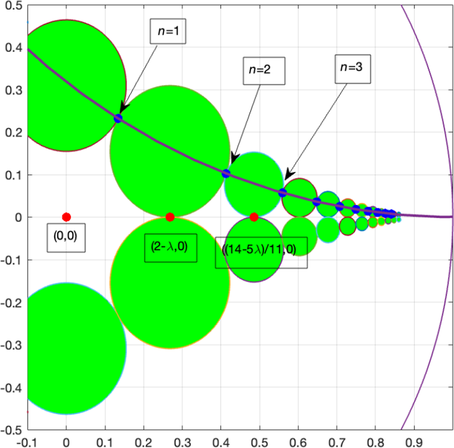
$F_{k,n}(\partial \mathbb D)$
 , see the blue points in Figure 3.
Points on the circles (colour online).

Figure 3 Long description
A mathematical plot on a grid with an x-axis from negative 0.1 to 0.9 and a y-axis from negative 0.5 to 0.5. Two symmetric rows of solid green circles are arranged above and below the x-axis.
Along the x-axis, three red dots are labeled with coordinates. From left to right, they are (0,0), (2 minus lambda, 0), and ((14 minus 5 lambda) all over 11, 0).
The upper sequence of circles is intersected by a purple curved line. Specific intersection points are marked with blue dots and labeled with callouts:
* n equals 1 points to the first blue dot on the largest upper circle.
* n equals 2 points to the second blue dot on the next smaller circle.
* n equals 3 points to the third blue dot on the third circle.
As the x-value increases, the circles in both the upper and lower sequences become progressively smaller, appearing to converge at a single point near x equals 0.9 on the x-axis. A large purple arc frames the right side of the plot, passing through the convergence point.
One can also check that for all
$n=1,2,\ldots ,$
 the points

lie on the circle of radius
$R_0=\unicode{x3bb} $
 centered at
$1+i\unicode{x3bb} $
 since

We now describe how to identify a third point in each circle
$F_{k,n} (\partial \mathbb D)$
 . This will allow us to prove items (2) and (3). These new points correspond to the red points in Figure 3. It follows by the arguments in the proof of item (1) that
$t_1:=2-\unicode{x3bb} \in \partial F_{k,1} (\partial \mathbb D)$
 . Moreover, the circle
$A_1:=\partial B(0, 2-\unicode{x3bb} )$
 is tangent to the ‘exterior’ tangent circles
$\partial B(1+\unicode{x3bb} i, \unicode{x3bb} )$
 and
$\partial B(1-\unicode{x3bb} i, \unicode{x3bb} )$
 (who are also tangent to each other). Since there is no triple tangency, we can apply Descartes’ theorem to find the curvature of the corresponding Apollonian circle (the second largest red circle inside
$\mathbb D$
 in Figure 4). Recall that Descartes’ theorem states that the curvatures
$k_1,k_2,k_3,k_4$
 of four circles with
$6$
 double tangencies and no triple tangency satisfy the equation

A sequence of Apollonian circles (colour online).

Figure 4 Long description
A geometric diagram plotted on an x-y axis ranging from -1 to 3 on the x-axis and -2 to 2 on the y-axis. Two large red circles with radius R sub 0 = lambda are positioned on the right, centered vertically at approximately y = 1.7 and y = -1.7. To the left, a large blue circle is centered at the origin. Inside this blue circle is a fractal gasket of smaller blue and green circles. A central red circle is labeled R sub 1 = 2 minus lambda. Moving right along the x-axis within the fractal, a smaller red circle is labeled R sub 2 = 1 all over (4 plus 3 lambda). Further right, an even smaller red circle is labeled R sub 3 = lambda all over (6 lambda plus 19). The circles decrease in size as they approach the point x = 1, where the large blue circle and the two large red circles meet.
In our case,

Thus, the curvature and radius of the next Apollonian circle
$A_2$
 is

Using this information, we find that

Thus, the following three distinct points

lie on
$F_{k,2}(\partial \mathbb D)$
 . Thus,

As in the proof of item (1), we see that if k is odd, then
$F_{k,2} (\mathbb D)=\overline F_{k+1, 2(\mathbb D)}$
 . Thus, item (2) follows because by (3.6), the disks
$\phi _{k,2} (\mathbb D)$
 are obtained by rotations of
$F_{1,2} (\mathbb D)$
 and
$F_{2,2} (\mathbb D)$
 .
We use Descartes’ formula (3.10) again to find the next Apollonian circle
$A_3$
 (the third largest red circle inside
$\mathbb D$
 in Figure 4). In this case, we have
$k_1=k_2=1/\unicode{x3bb} $
 and
$k_3=4+3\unicode{x3bb} $
 . Thus, the curvature and radius of
$A_3$
 are

Using this information, we find that

Thus, the following distinct points

lie in
$F_{k,3} (\partial\mathbb{D})$
 . Thus,

Therefore, item (3) follows arguing exactly as (in the end of) the proof of item (2).
Remark 3.2. If
$k_m$
 is the curvature of the Apollonian disk
$A_m$
 (the m largest red disk inside
$\mathbb D$
 in Figure 4), the curvature
$k_{m+1}$
 of the next Apollonian circle is given by

Thus, the radii of the Apollonian circles
$A_m$
 form a decreasing sequence
$(R_n)_{n \in {\mathbb {N}}}$
 . One can then show that the sequence
$\{\text {radius } \, \phi _{k,n}(\mathbb D)\}_{n \in {\mathbb {N}}}$
 is also decreasing.
The first step in bounding the distortion constant of
$\mathcal {A}$
 is obtaining an upper bound for the distortion of the maps
$\phi _{k,n}, (k,n) \in I$
 .
Proposition 3.3. For every
$(k,n) \in I$
 :

where

Proof. We saw in the proof of Proposition 3.1 that the map

has matrix representation

Recall that any Möbius transformation

has a matrix representation

and

Therefore,

where

From basic complex analysis, we know that the minimum and maximum of
$|z-A|$
 on the circle
$|z-z_0|=r$
 are attained at

and

respectively, and the minimum and maximum are

and

In our situation, we have
$A=-d/c$
 ,
$r=1$
 , and
$z_0=0$
 , and as a result,

Using that
$e^{i \theta _k}=-1/2\pm ({\lambda }/{2})i$
 for
$\theta _k=\pm ({2\pi }/{3})$
 , we have

Thus,

It remains to show that

For
$n\in [t_{\mathrm {min}},\infty )$
 with
$t_{\mathrm {min}}>0$
 , we have

and as a result, for
$n\in [t_{\mathrm {min}},\infty )$
 ,

Thus, for example, for
$t_{\mathrm {min}}=23$
 , that is for
$n\in [23,\infty )$
 , we have

and checking directly for
$n=1,2,\ldots ,22$
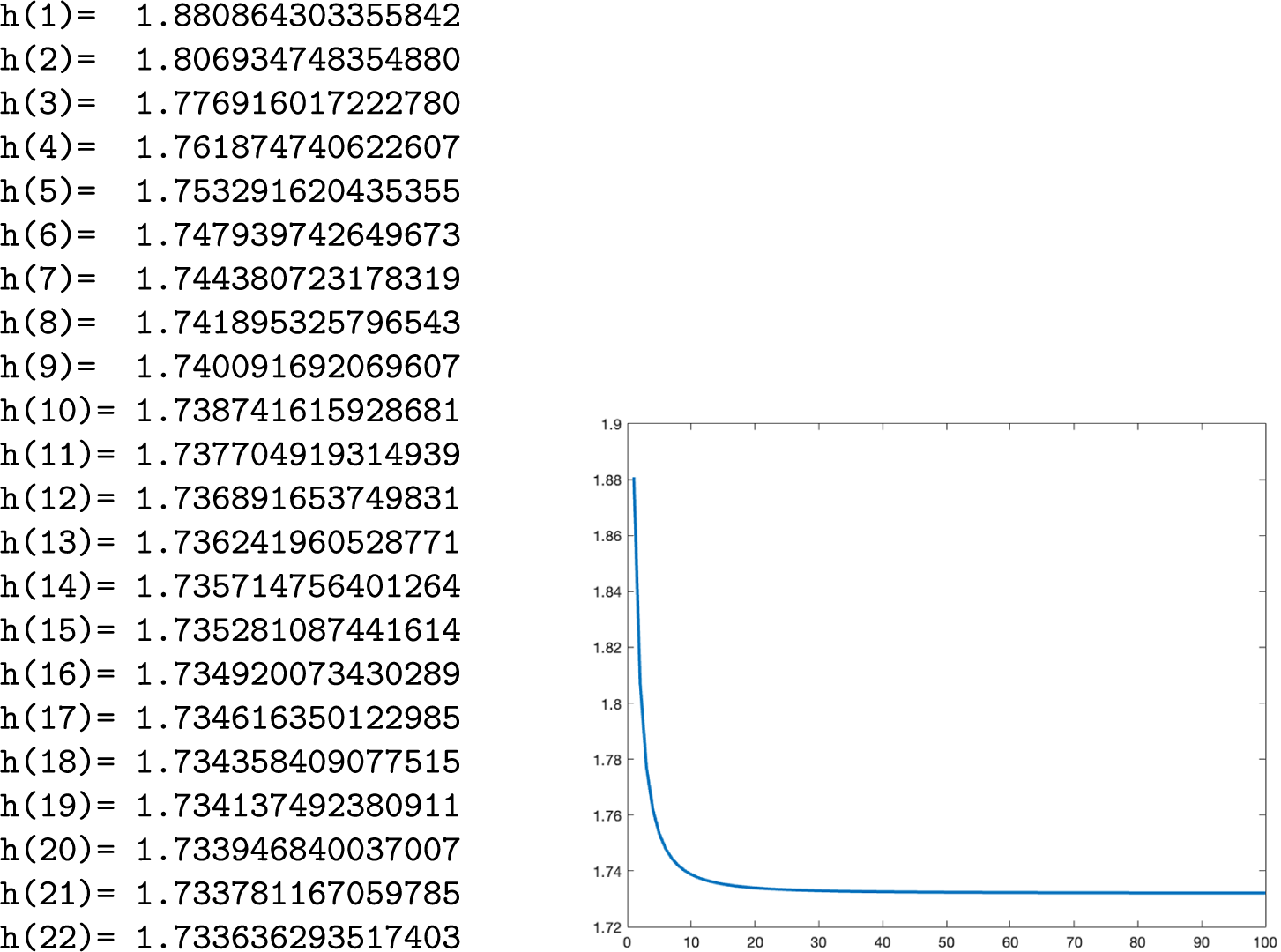
 , we have Figure 5.
The graph of
$h: \mathbb R^+ \to \mathbb R^+$
 (colour online).

Figure 5 Long description
The left panel contains a vertical list of 22 values for the function h(n) where n ranges from 1 to 22. The values start at h(1) = 1.880864303355842 and decrease steadily, reaching h(22) = 1.733636293517403.
The right panel is a line graph. The vertical y-axis ranges from 1.72 to 1.9 in increments of 0.02. The horizontal x-axis ranges from 0 to 100 in increments of 10. A solid blue line begins at approximately y = 1.88 when x is near 0. The curve shows a sharp exponential-like decay between x = 0 and x = 10, dropping toward the 1.74 mark. From x = 20 to x = 100, the curve flattens out, representing an asymptotic approach to a value just above 1.73.
Thus, we have established (3.12) and the proof is complete.
Remark 3.4. Interestingly,

where we used that
$\theta _k=\pm {2\pi }/{3}$
 and
$\unicode{x3bb} =\sqrt {3}$
 .
We can now use Propositions 3.1 and 3.3 to obtain the desired distortion bounds.
Proposition 3.5. If
$\omega \in I^\ast $
 , then

If
$\omega \in I_{n>1}^\ast $
 , then

If
$\omega \in I_{n>2}^\ast $
 , then

Proof. Let
$z,w \in \mathbb D$
 . We first prove (3.13). Let
$\omega \in I^n$
 . If
$n=1$
 , then (3.13) follows from Proposition 3.3. Thus, we can assume that
$|\omega |\geq 2$
 and we set
$g=\phi _{\omega _1} \circ \cdots \circ \phi _{\omega _{n-1}}$
 . Then, by Proposition 3.3,

We now estimate

We consider two cases. First, assume that
$\omega _n=(k,1)$
 for some
$k=1,\ldots ,6$
 . In that case, Proposition 3.1 implies that
$\tilde {z}:=\phi _{\omega _n}(z)$
 and
$\tilde {w}:=\phi _{\omega _n}(w)$
 lie in a disk
$B(\xi ,({2 \unicode{x3bb} -3})/{3})$
 such that
$\xi \in \partial B(0, ({4 \unicode{x3bb} -6})/{3})$
 . It follows that g is holomorphic (and injective) in
$B(\xi ,1+\unicode{x3bb} -|\xi |)$
 . By Koebe’s distortion theorem, see e.g. [Reference Urbański, Roy and Munday20, Theorem 23.1.6], (for
$r=({2 \sqrt {3}-3})/{3}$
 and
$R=1+\unicode{x3bb} -({4 \unicode{x3bb} -6})/{3}$
 ), we get

Therefore,

If
$\omega _n=(k,m)$
 for some
$m>1$
 and
$k=1,\ldots ,6$
 , then Proposition 3.1 and Remark 3.2 imply that
$\tilde {z},\tilde {w}$
 lie in a disk
$B(\zeta , \tilde {r})$
 such that
$B(\zeta ,\tilde {r}) \subset \mathbb D$
 and

Thus, we can apply Koebe’s distortion theorem in the disk
$B(\zeta , \unicode{x3bb} )$
 , since
$B(\zeta , \unicode{x3bb} ) \subset B(0,1+\unicode{x3bb} )$
 . Thus, for
$\tilde {R}=\unicode{x3bb} $
 ,

and

Note that (3.13) follows by (3.18) and (3.20). Moreover, (3.20) implies (3.14).
It remains to show (3.15). Note that in that case,
$\omega _1=(k,m)$
 for some
$m>2$
 and
$k=1,\ldots ,6$
 . Therefore, Proposition 3.1 and Remark 3.2 imply that
$\tilde {z},\tilde {w}$
 lie in a disk
$B(\eta , r')$
 such that
$B(\eta ,r') \subset \mathbb D$
 and

Applying Koebe’s distortion theorem in the disk
$B(\eta , \unicode{x3bb} )$
 (with
$r'$
 as above and
$R'=\unicode{x3bb} $
 ) gives

Therefore,

We have thus established (3.15) and the proof of the proposition is complete.
4 The dimension spectrum of the Apollonian gasket
Let
$\mathcal {S}=\{\phi _i:X \to X\}_{i \in I}$
 be a CIFS. If
$F \subset I$
 , we let
$\mathcal {S}_F=\{\phi _i: X \to X\}_{i \in F}$
 and we denote
$J_{\mathcal {S}_F}:=J_F$
 . We also denote the topological pressure of the subsystem
$\mathcal {S}_F$
 by
$P_{\mathcal {S}_F}:=P_F$
 . Recall that the dimension spectrum of
$\mathcal {S}$
 is defined as

We now state some facts from [Reference Chousionis, Leykekhman and Urbański3] that are essential in our approach. We say that a well-ordering
$\prec $
 on the alphabet I is natural (with respect to
$\mathcal {S}$
 ) if

Moreover, if
$I=\{i_n\}_{n \in {\mathbb {N}}}$
 is an enumeration respecting
$\prec $
 , we let

The following proposition is used repeatedly in our proof.
Proposition 4.1. [Reference Chousionis, Leykekhman and Urbański3, Proposition 6.17]
Let
$\mathcal {S}=\{\phi _i: X \to X\}_{i \in I}$
 be a CIFS. Let K be as in (2.1) and let
$I=\{i_n\}_{n \in {\mathbb {N}}}$
 be an enumeration of I according to a natural order
$\prec $
 . Suppose that there exist
$t_1 \leq t_2 \leq h(\mathcal {S})$
 and
$d \in {\mathbb {N}}$
 such that:
-
(1) $P_{I(d)}(t_1) \leq 0$
; -
(2) $\sum _{n \geq k+1} \| \phi _{i_n}'\|_\infty ^{t_2} \geq K^{2t_2} \|\phi _{i_k}'\|^{t_2}_\infty $
for all
$k \geq d+1$
.


Then,
$[t_1,t_2] \subset DS(\mathcal {S})$
 .
We now turn our attention to the Apollonian system
$\mathcal {A}$
 ; see (3.1). Recall that the alphabet of
$\mathcal {A}$
 is

We define the following well ordering of I:

Proposition 4.2. The well ordering defined in (4.1) is natural, that is,

Proof. In [Reference Chousionis, Leykekhman, Urbański and Wendt5], we showed that for all
$k=1,\ldots ,6$
 and
$n \in {\mathbb {N}}$
 ,

Therefore, it suffices to show that
$G: {\mathbb {N}} \to {\mathbb {N}}$
 is decreasing. We first compute the derivative of G:

To show that the derivative is negative, it is sufficient to show that

for all
$n\geq 1$
 . Using that for
$n_{\mathrm {min}}\le n<\infty $
 , the estimate

already holds for
$n_{\mathrm {min}}=3$
 , by checking directly for
$n=1,2$
 , we find

The proof is complete.
Since

(4.2) implies that for any
$(k,n) \in I$
 ,

Therefore, (2.6) implies that

Theorem 4.1. The Apollonian system
$\mathcal {A}$
 has full dimension spectrum; that is,

Proof. We first note that since
$\theta (\mathcal {A})=1/2$
 , [Reference Mauldin and Urbański12, Theorem 6.2] implies that

We use several subsystems of
$\mathcal {A}$
 of the form
$\mathcal {A}_S$
 where
$S \subset {\mathbb {N}}$
 ; recall (3.3) for their definition. We let
$E=\{e_n\}_{n \in {\mathbb {N}}}$
 be an enumeration of the alphabet
$I=\{(k,n):k=1,\ldots ,6, \ n \in {\mathbb {N}}\}$
 with respect to the natural order
$\prec $
 defined in (4.1). Since, by (4.2),
$\|\phi ^{\prime }_{k,n}\|$
 does not depend on k, we let
$\phi _n:=\phi _{k,n}$
 ,
$k=1,\ldots , 6$
 . Note that

where
$\lceil x \rceil $
 denotes the least integer greater than or equal to x. We repeatedly use the following corollary of Proposition 4.1.
Corollary 4.3. Let
$F \subset {\mathbb {N}}$
 and let
$\tilde {F}$
 be a finite initial subset of F. Let
$K_F$
 be a distortion constant for
$\mathcal {A}_{F}$
 . If
$0<t_1<t_2 \leq \dim_H (J_{\mathcal{A}_F})$
 and
-
(1) $\dim_H (J_{\mathcal{A}_{\tilde{F}}})\leq t_1$
, -
(2) $6 \sum_{n\in F: n>M} \|\phi'_n\|^{t_2}_{\infty} \geq K^{2t_2}_{F} \|\phi'_M\|^{t_2}_\infty \mbox{ for all }M \in F \text{ such that }M > \max \tilde{F},$


then
$[t_1,t_2] \subset DS(\mathcal {A_{\tilde {F}}})\subset DS(\mathcal {A})$
 .
Proof. We let

Let
$(\epsilon _i)_{i \in {\mathbb {N}}}$
 be an enumeration of
$I_F$
 with respect to the natural order
$\prec $
 , as in (4.1). Clearly,
$\{1,\ldots , 6\} \times \tilde {F}$
 corresponds to the initial segment
$I(q)$
 of
$\tilde {I}$
 , where
$q= 6 \cdot \sharp F$
 . Therefore, our claim follows by Proposition 4.1 if we show that

Let
$d \geq q+1$
 . If
$\epsilon_d=(k,M)$
 then

Upper and lower bounds for the Hausdorff dimension of the subsystems of
$\mathcal {A}$
 used in the proof of Theorem 4.1.

Table 2 Long description
The table consists of three columns and four data rows.
Column headers from left to right are: Subsystem, Lower bound for dim sub H, and Upper bound for dim sub H.
Row 1: Subsystem A sub 1. Lower bound is s sub 1. Upper bound is s sub 1.
Row 2: Subsystem A sub 2. Lower bound is s sub 2. Upper bound is s sub 2.
Row 3: Subsystem A sub 3. Lower bound is s sub 3. Upper bound is s sub 3.
Row 4: Subsystem A sub 4. Lower bound is s sub 4. Upper bound is s sub 4.
The table demonstrates that for each listed subsystem from A sub 1 to A sub 4, the lower and upper bounds for the Hausdorff dimension are identical, represented by the corresponding s sub i value.
By the integral test,

By (4.7) and the fact that the function
$x \to {x^{2t}}/({(x+1)^{2t-1}})$
 is increasing for
$x>0$
 , we deduce that

implies

Moreover, since the function
$t \to {6\, (N+1)}/({2t-1}) (({N}/{N+1})^2 \ {0.45}/{3.821 \, K^2 } )^t$
 is decreasing for
$t>1/2$
 , if
$t>s>1/2$
 ,

We now use Corollary 4.3 to find a chain of intervals in
$DS(\mathcal {A})$
 whose union contains
$[1/2, \dim _{H}(J_{\mathcal {A}})]$
 . Starting with an interval which contains
$\dim _{H}(J_{\mathcal {A}})$
 , we use a bootstrapping method to reach
$1/2$
 with overlapping intervals in
$DS(\mathcal {A})$
 . Our computational method from [Reference Chousionis, Leykekhman, Urbański and Wendt5] is absolutely essential in this approach and is applied repeatedly to derive lower and upper bounds for the Hausdorff dimension of various subsystems of
$\mathcal {A}$
 , see Table 2. For steps 1–16, we use the distortion constant
$K=K_{\mathcal {A}}=5.900319$
 as in (3.13). For steps 17 and 18, we work with the dimension spectrum
$\mathcal {A}_{n>2}$
 , so we use the improved distortion constant

as in (3.15). We describe in detail the first four steps.
Step 1. We know that

For
$t_2=1.3057$
 , (4.8) holds for
$N=454$
 . We then check that

holds for
$M \geq 27$
 . Thus, (4.9) holds for
$t_2=1.3057$
 and
$N=27$
 . Applying the method we developed in [Reference Chousionis, Leykekhman, Urbański and Wendt5], we obtain

Therefore, Corollary 4.3 implies that

Step 2. Arguing as in Step 1 and using (4.10), we find that condition (4.9) holds for
$t_2=1.3001$
 and
$N=26$
 . We then find that

Therefore, Corollary 4.3 implies that

which, combined with (4.11), implies that

Step 3. In this step, we consider the subsystem
$\mathcal {A}_{n \neq 11,12}$
 , that is, the Apollonian subsystem with alphabet
$\{(k,n): k=1,\ldots , 6, \, n\in {\mathbb {N}} \setminus \{ 11,12\}\}$
 , whose Hausdorff dimension satisfies

Arguing as in Step 1 and using (4.10), we find that condition (4.9) holds for
$t_2=1.300$
 and
$N=26$
 . Moreover,

where
$F_3=\{n\in {\mathbb {N}}: n\leq 25, n \neq 11,12\}$
 . Therefore, Corollary 4.3 implies that

which, combined with (4.12), implies that

Step 4. In this step, we consider the subsystem
$\mathcal {A}_{n \neq 11,12,13,14,15}$
 whose dimension satisfies

Arguing as in Step 1 and using (4.10), we find that condition (4.9) holds for
$t_2=1.295$
 and
$N=26$
 . Moreover,

where
$F_4=\{n=1,\ldots ,10,16,\ldots ,25\}$
 . Therefore, Corollary 4.3 implies that

which, combined with (4.13), implies that

We continue in the same way until we obtain an interval which contains
$1/2$
 . The details of the remaining steps (5–18) can be found in Table 1.
Remark 4.4. The estimate for the size of the best distortion constant
$K_{\mathcal {A}}$
 plays a crucial role in our argument. A better estimate can lead to a reduced number of steps. However, the estimate we obtained in Proposition 3.5 was sufficient for obtaining the first crucial step. One also may notice that the iterative argument makes rather small progress initially and then speeds up. We have also not tried to optimize the number of steps. There are many other choices for subsystems and it is likely that a different choice of subsystems would lead to the result faster.
Acknowledgements
V.C. and D.L. were supported by NSF grant 2513639. V.C. was supported by Simons Foundation Collaboration grant 521845 and by NSF grant 2247117. M.U. was supported by Simons Foundation Collaboration grant 581668.