1 Introduction
Dynamics of a drop has been studied from theoretical and experimental perspectives as a classical topic in fluid mechanics for a long time. For example, its natural frequencies in the absence of any impurity was first derived a century ago (Rayleigh Reference Rayleigh1879). Research on this topic was later enriched by several mathematical works (Chandrasekhar Reference Chandrasekhar1959; Miller & Scriven Reference Miller and Scriven1968; Prosperetti Reference Prosperetti1980; Strani & Sebetta Reference Strani and Sebetta1984, Reference Strani and Sebetta1988; Lundgren & Mansour Reference Lundgren and Mansour1988; Trinh, Marston & Robey Reference Trinh, Marston and Robey1988; Basaran Reference Basaran1992; Bostwick & Steen Reference Bostwick and Steen2009, Reference Bostwick and Steen2013; Jiri, Lucie & Jaroslav Reference Jiri, Lucie and Jaroslav2013) and experimental investigations (Epstein & Plesset Reference Epstein and Plesset1950; Apfel et al. Reference Apfel, Tian, Jankovsky, Shi, Chen, Holt, Trinh, Croonquist, Thornton and Sacco1997; Lauterborn & Ohl Reference Lauterborn and Ohl1997; Obreschkow et al. Reference Obreschkow, Kobel, Dorsaz, Bosset, Nicollier and Farhat2006). Still, interfacial waves in a bubble-laden multiphase droplet have been analysed with a compact mathematical treatment only recently (Bhattacharya Reference Bhattacharya2016). This article generalizes the recent formulation to describe the frequency spectra of a pulsating drop for an arbitrary position of the embedded cavity.
This paper describes a new analysis for interfacial pulsation of a compound droplet. The majority of the relevant prior studies on this topic only focused on a concentric geometry under unperturbed conditions addressing problems which can be divided into two categories. Firstly, there have been a number of investigations on oscillations in a thin liquid shell engulfing an interior fluid with different properties (Patzer & Homsy Reference Patzer and Homsy1975; Kawano, Shirai & Nagasaka Reference Kawano, Shirai and Nagasaka2007). Secondly, several numerical simulations (Tsamopoulos & Brown Reference Tsamopoulos and Brown1983; Pelekasis, Tsamopoulos & Manolis Reference Pelekasis, Tsamopoulos and Manolis1991) have also revealed time-dependent evolution of the interfaces under an axisymmetric perturbation. Apart from these two broad groups, we located a couple of articles where a predominantly analytical procedure revealed dynamics in thick liquid shells. The first of these uses approximate flow solutions to predict stability features of the dynamic behaviour (Landman Reference Landman1985). In contrast, the second one applies perturbation theory to show the appearance of fine spectral structures under the limit of small displacement of the void from a concentric position (Lyubimov et al. Reference Lyubimov, Konovalov, Lyubimova and Egry2012). However, such formulation is not valid for a large separation between the centres of the drop and the bubble under unperturbed conditions. Thus, none of these works attempted to accurately find the exact frequency spectra of the pulsating system for arbitrary size and position of the embedded cavity under arbitrary asymmetric perturbations.
This article describes the frequency spectra for small-amplitude interfacial pulsation of the bubble-laden drop under the low capillary number limit. The underlying assumptions are exactly same as Rayleigh’s renowned work (Rayleigh Reference Rayleigh1879) which is still technologically relevant in modern times despite its classical nature. We show how Rayleigh’s spectra modifies due to the existence of a bubble inside the liquid. Thus, our analysis is a generalization of the well-known past results used in a wide range of research fields.
Determination of the aforementioned frequency spectra can facilitate several scientific and technological developments. The most important application of our theory is based on its potential in the realization of an important detection technique. Typically, liquid droplets are optically opaque. As a result, it is nearly impossible to visualize their interior by direct observation. This inability prohibits characterization of any bubble or particle residing inside the domain. Our analysis provides a novel solution to this problem. Accordingly, one can record the interfacial pulsation of a suspended drop with a high-speed camera, and detect any embedded species from the frequency spectra revealed by the stored data. Such explorative capability can provide crucial information about spraying techniques (Schwabe et al. Reference Schwabe, Rubin-Zuzic, Zhdanov, Ivlev, Thomas and Morfill2009), particle depositions (Yunker et al. Reference Yunker, Still, Lohr and Yodh2011), fuel combustion (Pelosi & Gany Reference Pelosi and Gany2012) and material processing (Minemawari et al. Reference Minemawari, Yamada, Matsui and Tsutsumi2011). Consequently, it can help in quality control and improvement of several combustive and manufacturing systems.
Apart from the detection capability, if frequency spectra of a multiphase droplet are known, they can be used to find the resonance features for the dynamic system. As a result, a suitable sonic wave can be identified so that it can resonate with the drop, leading to its acoustically assisted controlled break up (Taller, Go & Chang Reference Taller, Go and Chang2012). This can be a means to enhance the efficiency of combustion processes (Iyer, Abraham & Magi Reference Iyer, Abraham and Magi2002).
Also, our study can lead to the analysis of the surface pulsation of voids generated during cavitation. Distortion in interfacial shape described by Rayleigh’s frequency (Rayleigh Reference Rayleigh1879) is only relevant for incompressible bubbles or drops. In contrast, cavitation is modelled by the Rayleigh–Plesset equation (Rayleigh Reference Rayleigh1917; Plesset Reference Plesset1949) revealing volume fluctuation in a spherically symmetric bubble. Accordingly, the frequencies for the first few interfacial modes are much smaller than the typical value associated with a compressible system. Still, resonance between the volumetric waves and higher interfacial modes can potentially impact the cavitation process, although this is not the subject of our present paper.
The key feature of the system considered in our analysis is the appearance of the bubble at an arbitrary eccentric location around which it undergoes small-amplitude fluctuations. The relative velocity between the centres of the cavity and the drop is small so that the former remains in the vicinity of its original position throughout the time scale of interest. The resulting flow satisfies the unsteady inviscid equation which is solved in terms of singular and regular harmonic functions. Their unknown time-dependent amplitudes are then described in a matrix formulation by exploiting the surface tension dictated boundary conditions at the external surface and the liquid–bubble interface. The appropriate characteristic relations from the derived matrices ultimately yield the frequencies of different wave modes for a given average position of the embedded cavity.
The article is organized in the following way. In § 2, the flow solution and the matrix formulation reveal how finer structures in the frequency spectra form bands for an eccentrically placed bubble, and how their values converge with the number of basis functions. Section 3 presents an asymptotic theory under the limit of a small perturbation in the position of the cavity to independently verify our simulation. In § 4, we identify key features in the fine spectral structure from their variation with the position of the bubble and outline an algorithm to detect their size and location if the frequencies are known. Finally, in § 5, the article is summarized and the conclusions are drawn.
2 Natural frequencies for different modes of interfacial waves
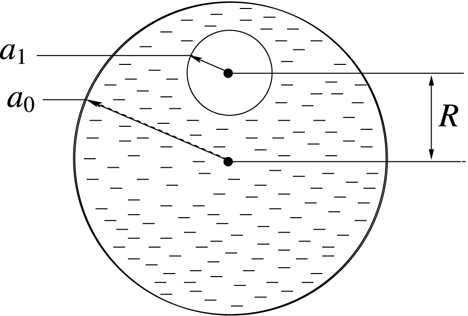
Our analysis considers a spherical bubble of radius
 $a_{1}$
inside a spherical drop of radius
 $a_{0}$
with their centres separated by an average distance
 $R$
. The void appears at the radial position
 $R$
and remains in vicinity of this point while undergoing small-amplitude fluctuations. The finite value of
 $R$
distinguishes our work from previous articles such as Landman (Reference Landman1985), Lyubimov et al. (Reference Lyubimov, Konovalov, Lyubimova and Egry2012). The density of the surrounding atmosphere and the air trapped in the cavity is assumed to be negligible. The viscosity and density for the fluid domain are denoted by
 $\unicode[STIX]{x1D707}$
and
 $\unicode[STIX]{x1D70C}$
, respectively. The surface tension coefficient for the liquid–air interface is represented by
 $\unicode[STIX]{x1D6FE}$
. Our main focus in this article is to describe the natural frequencies of the prominent modes of vibrations as functions of
 $R$
and the size ratio
 $\tilde{a}=a_{1}/a_{0}$
. The system is schematically described in figure 1.
Schematic of a spherical drop under unperturbed condition with a spherical bubble undergoing small-amplitude fluctuations in the vicinity of an eccentric location.

We assume the characteristic amplitude
 $A_{s}$
for the surface perturbation is small compared to
 $a_{0}$
. Then, the velocity scale
 $A_{s}\sqrt{\unicode[STIX]{x1D6FE}/(\unicode[STIX]{x1D70C}a_{0}^{3})}$
ensures the ratio between the convective and temporal accelerations to be of the order of
 $A_{s}/a_{0}$
. Hence, the nonlinear convective inertia remains insignificant, enabling linearization of the flow equations. Moreover, the ratio of viscous and interfacial forces is given by the capillary number
 $Ca=\unicode[STIX]{x1D707}A_{s}/\sqrt{\unicode[STIX]{x1D6FE}\unicode[STIX]{x1D70C}a_{0}^{3}}$
. Similarly, the Bond number
 $B_{o}=g\unicode[STIX]{x1D70C}a_{0}^{2}/\unicode[STIX]{x1D6FE}$
represents the relative importance of gravity
 $g$
compared to surface tension. For millimetre size water droplets,
 $Bo$
is approximately
 $0.1$
and
 $Ca$
is of similar order when
 $A_{s}/a_{0}$
is less than
 $0.1$
. For other typical liquids, these values are even lower. This is why our analysis presumes that both
 $Ca$
and
 $Bo$
are small for our system.
Accordingly, simplified conservation equations relate pressure
 $p$
and displacement
 $\boldsymbol{s}$
:
 $$\begin{eqnarray}\unicode[STIX]{x1D70C}\frac{\unicode[STIX]{x2202}^{2}\boldsymbol{s}}{\unicode[STIX]{x2202}t^{2}}=-\unicode[STIX]{x1D735}p,\quad \unicode[STIX]{x1D6FB}^{2}p=0,\end{eqnarray}$$
where
 $t$
is time. In the absence of any viscous stress, the boundary conditions at two eccentrically placed spherical free surfaces of the liquid domain become
 $$\begin{eqnarray}p|_{r_{0}=a_{0}}=-\unicode[STIX]{x1D6FE}\left[\frac{2\boldsymbol{s}\boldsymbol{\cdot }\hat{\boldsymbol{n}}_{0}}{a_{0}^{2}}+\unicode[STIX]{x1D6FB}_{s}^{2}(\boldsymbol{s}\boldsymbol{\cdot }\hat{\boldsymbol{n}}_{0})\right],\quad p|_{r_{1}=a_{1}}=-\unicode[STIX]{x1D6FE}\left[\frac{2\boldsymbol{s}\boldsymbol{\cdot }\hat{\boldsymbol{n}}_{1}}{a_{1}^{2}}+\unicode[STIX]{x1D6FB}_{s}^{2}(\boldsymbol{s}\boldsymbol{\cdot }\hat{\boldsymbol{n}}_{1})\right].\end{eqnarray}$$
Here,
 $r_{0}$
and
 $r_{1}$
are the radial coordinates of the spherical systems with origins at the centres of the drop and the bubble, respectively. The unit normal vector pointing away from the liquid domain at the
 $i$
th surface is
 $\hat{\boldsymbol{n}}_{i}$
, and the gradient along the spherical surface is given by
 $\unicode[STIX]{x1D735}_{s}$
. We find the solution of equation (2.1a,b
), and satisfy equation (2.2) in a matrix form to characterize the frequency spectra for different modes of the pulsation at the involved surfaces.
2.1 Field solutions
The continuity relation in equation (2.1a,b
) implies that the pressure
 $p$
is a harmonic field. Similarly, the momentum equation shows that
 $\boldsymbol{s}$
is a gradient of harmonic functions. Also, the presence of two interfaces indicates that two different classes of spherical basis solutions for the Laplace equation should be considered to describe
 $p$
and
 $\boldsymbol{s}$
. Firstly, as the fluid domain is truncated by the outer surface, the fields should include regular solutions which remain finite in a finite domain but become infinite far away from the origin. Moreover, the presence of the bubble allows us to take into account singular solutions with an infinite value at the centre of the cavity, which is precluded from the domain of interest by the inner interface. Thus, we draw inspiration from Stokesian dynamics (Sangani & Mo Reference Sangani and Mo1996; Bhattacharya, Mishra & Bhattacharya Reference Bhattacharya, Mishra and Bhattacharya2010; Navardi & Bhattacharya Reference Navardi and Bhattacharya2013) to propose a general solution for equation (2.1a,b
)
 $$\begin{eqnarray}\displaystyle & \displaystyle p=-\unicode[STIX]{x1D70C}\left[\mathop{\sum }_{lm}\ddot{\unicode[STIX]{x1D6FC}}_{lm}^{0+}(t)\unicode[STIX]{x1D719}_{lm}^{0+}(\boldsymbol{r})+\mathop{\sum }_{l^{\prime }m^{\prime }}\ddot{\unicode[STIX]{x1D6FC}}_{l^{\prime }m^{\prime }}^{1-},(t)\unicode[STIX]{x1D719}_{l^{\prime }m^{\prime }}^{1-}(\boldsymbol{r})\right], & \displaystyle\end{eqnarray}$$
 $$\begin{eqnarray}\displaystyle & \displaystyle \boldsymbol{s}=\unicode[STIX]{x1D735}\left[\mathop{\sum }_{lm}\unicode[STIX]{x1D6FC}_{lm}^{0+}(t)\unicode[STIX]{x1D719}_{lm}^{0+}(\boldsymbol{r})+\mathop{\sum }_{l^{\prime }m^{\prime }}\unicode[STIX]{x1D6FC}_{l^{\prime }m^{\prime }}^{1-}(t)\unicode[STIX]{x1D719}_{l^{\prime }m^{\prime }}^{1-}(\boldsymbol{r})\right]. & \displaystyle\end{eqnarray}$$
Here,
 $\unicode[STIX]{x1D719}_{lm}^{i+}$
and
 $\unicode[STIX]{x1D719}_{lm}^{i-}$
are the regular and singular basis functions in spherical coordinates with origin at the centre of the
 $i$
th interface. Accordingly, these are defined by
 $$\begin{eqnarray}\unicode[STIX]{x1D719}_{lm}^{0+}=Y_{lm}^{(0)}\left(\frac{r_{0}}{a_{0}}\right)^{l},\quad \unicode[STIX]{x1D719}_{lm}^{0-}=Y_{lm}^{(0)}\left(\frac{a_{0}}{r_{0}}\right)^{l+1},\quad \unicode[STIX]{x1D719}_{lm}^{1+}=Y_{lm}^{(1)}\left(\frac{r_{1}}{a_{1}}\right)^{l},\quad \unicode[STIX]{x1D719}_{lm}^{1-}=Y_{lm}^{(1)}\left(\frac{a_{1}}{r_{1}}\right)^{l+1},\end{eqnarray}$$
with
 $Y_{lm}^{(i)}$
being the spherical harmonics on the surface of the
 $i$
th sphere where the angular variations are defined by two usual quantum numbers
 $l=1,2,3,\ldots$
and
 $m=0,\pm 1,\pm 2,\ldots ,\pm l$
. The corresponding time-dependent amplitudes are
 $\unicode[STIX]{x1D6FC}_{lm}^{i\pm }$
, and overdots in equation (2.3) represent second-order temporal derivatives.
We use only
 $\unicode[STIX]{x1D719}_{lm}^{0+}$
and
 $\unicode[STIX]{x1D719}_{lm}^{1-}$
in (2.3) and (2.4). This is because the regular solution appearing due to the truncation of the domain by the external surface should be naturally expanded around its centre. Similarly, the singular function introduced due to the exclusion of the bubble volume should be expressed in the corresponding spherical coordinates. Still, the solutions of
 $p$
and
 $\boldsymbol{s}$
can have alternative representations than the one presented in (2.3) and (2.4). Such flexibility exists due to two transformation relations.
The regular basis functions can be expanded in Taylor series equating these to a linear combination of spherical solutions centred around another point. Hence,
 $$\begin{eqnarray}\unicode[STIX]{x1D719}_{lm}^{0+}=\mathop{\sum }_{l^{\prime }m^{\prime }}\unicode[STIX]{x1D719}_{l^{\prime }m^{\prime }}^{1+}T_{r}(R|l^{\prime }m^{\prime },lm),\end{eqnarray}$$
where
 $T_{r}(R|l^{\prime }m^{\prime },lm)$
are the transformation coefficients which represent the Taylor series expansion of
 $\unicode[STIX]{x1D719}_{lm}^{0+}$
at the centre of the cavity. At this point, we choose the
 $z$
axis to be aligned with the line joining the centres of the drop and the bubble. Under such a construction,
 $T_{r}$
uncouples
 $m$
and
 $m^{\prime }$
, and assumes the following simplified form
 $$\begin{eqnarray}T_{r}(R|l^{\prime }m^{\prime },lm)=T_{r}(R,m|l,l^{\prime })\unicode[STIX]{x1D6FF}_{mm^{\prime }}=\tilde{a}^{l^{\prime }}\frac{\tilde{R}^{(l-l^{\prime })}}{(l-l^{\prime })!}\sqrt{\frac{(2l+1)(l-m)!(l+m)!}{(2l^{\prime }+1)(l^{\prime }-m)!(l^{\prime }+1)!}}\unicode[STIX]{x1D6FF}_{mm^{\prime }}.\end{eqnarray}$$
Here,
 $\tilde{a}=a_{1}/a_{0}$
,
 $\tilde{R}=R/a_{0}$
and
 $\unicode[STIX]{x1D6FF}_{mm^{\prime }}$
is the Kronecker delta implying the block diagonalization of different azimuthal modes defined by
 $m$
.
Similar transformation between the singular solutions can also be derived using Taylor series expansion, although the presence of the singularity limits its validity by the convergence radius. Hence, for points outside the sphere of radius
 $R$
around the centre of the drop:
 $$\begin{eqnarray}\unicode[STIX]{x1D719}_{l^{\prime }m^{\prime }}^{1-}=\mathop{\sum }_{lm}\unicode[STIX]{x1D719}_{lm}^{0-}T_{f}(lm,l^{\prime }m^{\prime }|R).\end{eqnarray}$$
The new transformation coefficients are obtained as
 $$\begin{eqnarray}T_{f}(lm,l^{\prime }m^{\prime }|R)=T_{f}(l,l^{\prime }|R,m)\unicode[STIX]{x1D6FF}_{mm^{\prime }}=\tilde{a}T_{r}(l^{\prime },l|R,m)\unicode[STIX]{x1D6FF}_{mm^{\prime }},\end{eqnarray}$$
where the earlier choice of the
 $z$
-axis is taken for granted.
The complete description of the dynamics requires evaluation of the amplitudes
 $\unicode[STIX]{x1D6FC}_{lm}^{i\pm }(t)$
. This is achieved by satisfying the boundary conditions in (2.2), where we use the completeness of the solutions in (2.3) and (2.4) along with the flexibility given by (2.6)–(2.9).
2.2 Matrix formulation
We combine the boundary condition (2.2), the general solutions (2.3) and (2.4) and transformations (2.6)–(2.9) to derive two sets of ordinary differential equations describing
 $\unicode[STIX]{x1D6FC}_{lm}^{0+}$
and
 $\unicode[STIX]{x1D6FC}_{lm}^{1-}$
simultaneously. The first set of these relations comes from the surface tension dictated stress discontinuity at the outer surface of the drop
 $$\begin{eqnarray}\ddot{\unicode[STIX]{x1D6FC}}_{lm}^{0+}+\frac{\unicode[STIX]{x1D6FE}l}{\unicode[STIX]{x1D70C}a_{0}^{3}}(l^{2}+l-2)\unicode[STIX]{x1D6FC}_{lm}^{0+}=-\mathop{\sum }_{l^{\prime }m^{\prime }}T_{f}(lm,l^{\prime }m^{\prime }|R)\left[\ddot{\unicode[STIX]{x1D6FC}}_{l^{\prime }m^{\prime }}^{1-}-\frac{\unicode[STIX]{x1D6FE}}{\unicode[STIX]{x1D70C}a_{0}^{3}}(l+1)(l^{2}+l-2)\unicode[STIX]{x1D6FC}_{l^{\prime }m^{\prime }}^{1-}\right].\end{eqnarray}$$
The second group represents the same condition at the interface of the embedded bubble:
 $$\begin{eqnarray}\ddot{\unicode[STIX]{x1D6FC}}_{lm}^{1-}+\frac{\unicode[STIX]{x1D6FE}l}{\unicode[STIX]{x1D70C}a_{1}^{3}}(l+1)(l^{2}+l-2)\unicode[STIX]{x1D6FC}_{lm}^{1-}=-\mathop{\sum }_{l^{\prime }m^{\prime }}T_{r}(R|lm,l^{\prime }m^{\prime })\left[\ddot{\unicode[STIX]{x1D6FC}}_{l^{\prime }m^{\prime }}^{0+}-\frac{\unicode[STIX]{x1D6FE}}{\unicode[STIX]{x1D70C}a_{1}^{3}}(l^{2}+l-2)\unicode[STIX]{x1D6FC}_{l^{\prime }m^{\prime }}^{0+}\right].\end{eqnarray}$$
These equations should be considered for all possible
 $l$
and
 $m$
.
We cast equations (2.10) and (2.11) into a matrix form which has a block-diagonal structure, uncoupling mutual effects between two modes with different
 $m$
. Accordingly, one finds
 $$\begin{eqnarray}\displaystyle & & \displaystyle \left[\begin{array}{@{}cc@{}}[I] & [T^{f}(R,m)]\\ \hspace{0.0pt}[T^{r}(R,m)] & [I]\end{array}\right]\left\{\begin{array}{@{}c@{}}|\!\ddot{\unicode[STIX]{x1D6FC}}_{m}^{0+}\!\rangle \\ |\!\ddot{\unicode[STIX]{x1D6FC}}_{m}^{1-}\!\rangle \end{array}\right\}\nonumber\\ \displaystyle & & \displaystyle \quad +\,\frac{\unicode[STIX]{x1D6FE}}{\unicode[STIX]{x1D70C}a_{0}^{3}}\left[\begin{array}{@{}cc@{}}[D^{0}] & -[\tilde{T}^{f}(R,m)]\\ -[\tilde{T}^{r}(R,m)] & [D^{1}]\end{array}\right]\left\{\begin{array}{@{}c@{}}|\!\unicode[STIX]{x1D6FC}_{m}^{0+}\!\rangle \\ |\!\unicode[STIX]{x1D6FC}_{m}^{1-}\!\rangle \end{array}\right\}=\left\{\begin{array}{@{}c@{}}|\!0\!\rangle \\ |\!0\!\rangle \end{array}\right\}.\end{eqnarray}$$
Here, components in column
 $|\!\unicode[STIX]{x1D6FC}_{m}^{i\pm }\!\rangle$
are amplitudes for specific
 $m$
but different
 $l$
. Elements of square matrices
 $[T^{f}]$
and
 $[T^{r}]$
are the transformation coefficients
 $T_{f}(l,l^{\prime }|R,m)$
and
 $T_{r}(l,l^{\prime }|R,m)$
. Also,
 $[\tilde{T}^{f}]$
and
 $[\tilde{T}^{r}]$
are related to
 $[T^{f}]$
and
 $[T^{r}]$
 $$\begin{eqnarray}\tilde{T}_{ll^{\prime }}^{r}=\tilde{a}^{-3}l(l^{2}+l-2)T_{ll^{\prime }}^{r},\quad \tilde{T}_{ll^{\prime }}^{f}=\tilde{a}(l+1)(l^{2}+l-2)T_{l^{\prime }l}^{r},\end{eqnarray}$$
whereas
 $[D^{0}]$
and
 $[D^{1}]$
have only non-zero components in diagonal positions so that
 $$\begin{eqnarray}D_{ll^{\prime }}^{0}=l(l^{2}+l-2)\unicode[STIX]{x1D6FF}_{ll^{\prime }},\quad D_{ll^{\prime }}^{1}=\tilde{a}^{-3}(l+1)(l^{2}+l-2)\unicode[STIX]{x1D6FF}_{ll^{\prime }}.\end{eqnarray}$$
The identity operator in equation (2.12) is shown as
 $[I]$
.
We combine
 $|\!\unicode[STIX]{x1D6FC}_{m}^{0+}\!\rangle$
and
 $|\!\unicode[STIX]{x1D6FC}_{m}^{1-}\!\rangle$
into a single column notation
 $|\!\unicode[STIX]{x1D6FC}_{m}\!\rangle$
which is the transpose of
 $\{\langle \!\unicode[STIX]{x1D6FC}_{m}^{0+}\! |\langle \!\unicode[STIX]{x1D6FC}_{m}^{1-}\!|\}$
so that equation (2.12) can be written in a more concise form:
 $$\begin{eqnarray}[M(R,m)]|\!\ddot{\unicode[STIX]{x1D6FC}}_{m}\!\rangle +\,[S(R,m)]|\!\unicode[STIX]{x1D6FC}_{m}\!\rangle = |\!0\!\rangle ,\end{eqnarray}$$
where
 $$\begin{eqnarray}[M(R,m)]=\left[\begin{array}{@{}cc@{}}[I] & [T^{f}(R,m)]\\ \hspace{0.0pt}[T^{r}(R,m)] & [I]\end{array}\right],\quad [S(R,m)]=\left[\begin{array}{@{}cc@{}}[D^{0}] & -[\tilde{T}^{f}(R,m)]\\ -[\tilde{T}^{r}(R,m)] & [D^{1}]\end{array}\right].\end{eqnarray}$$
We refer to
 $[M(R,m)]$
and
 $[S(R,m)]$
as the mass and spring matrices, respectively. The spectra of the interfacial pulsation of the system are directly dependent on
 $[M(R,m)]$
and
 $[S(R,m)]$
. For a given
 $m$
, temporal variation in any
 $k$
th mode of vibration is expressed as a sinusoidal behaviour:
 $$\begin{eqnarray}|\!\unicode[STIX]{x1D6FC}_{km}(t)\!\rangle =\exp (\text{i}\unicode[STIX]{x1D714}_{km}t)|\!\unicode[STIX]{x1D6FC}_{km}(0)\!\rangle ,\end{eqnarray}$$
where
 $\unicode[STIX]{x1D714}_{km}$
is the corresponding natural frequency. When this variation is inserted into (2.15),
 $|\!\unicode[STIX]{x1D6FC}_{km}(0)\!\rangle$
and
 $\unicode[STIX]{x1D714}_{km}^{2}$
can be identified as the eigen vectors and eigen values of the matrix
 $[P]=[M]^{-1}[S]$
. In our computation, we construct
 $[M]$
,
 $[S]$
and
 $[P]$
for arbitrary bubble position
 $R$
and quantum number
 $m$
. Then, the eigen values of
 $[P]$
are calculated to reveal the prominent frequencies of the system.
It is to be noted here that the described matrix formulation reveals an inherent coupling between the dynamics of the two interfaces. This interdependence is quantified by the off-diagonal elements of
 $[M]$
and
 $[S]$
matrices represented by the blocks
 $[T^{f}]$
,
 $[T^{r}]$
,
 $[\tilde{T}^{f}]$
,
 $[\tilde{T}^{r}]$
. As the components of the off-diagonal blocks vary as power functions of
 $\tilde{a}$
, the effect of one surface on another becomes negligible for small void fractions. This is manifested in our prior work (Bhattacharya Reference Bhattacharya2016) where it is seen that deformability of the bubble is insignificant for
 $\tilde{a}<0.3$
. Such behaviour is corroborated by experimental studies also (Obreschkow et al.
Reference Obreschkow, Kobel, Dorsaz, Bosset, Nicollier and Farhat2006).
2.3 Test for spectral convergence
For a specific
 $m$
value,
 $l$
can be any positive integer as long as
 $l\geqslant |m|$
. Therefore,
 $[M]$
,
 $[S]$
and
 $[P]$
are infinite dimensional matrices in reality. However, for practical simulations, their dimensionality has to be truncated by enforcing a maximum value for
 $l$
given by
 $l_{mx}+|m|-1$
. This spectral truncation makes the dimensionality of all relevant matrices
 $2l_{mx}$
due to the
 $2\times 2$
block shown in (2.16). As a result, we expect
 $2l_{mx}$
number of eigen values for
 $[P]$
leading to the same number of natural frequencies.
For a concentric geometry, these are classified into
 $(+)$
and
 $(-)$
configurations in an earlier paper (Bhattacharya Reference Bhattacharya2016) accounting for a twofold increase in the number of possible modes compared to the pure drop analysed by Rayleigh. For
 $(+)$
states, the outer surface deforms relatively less, and maintains perfect alignment with the bubble. In contrast, the
 $(-)$
states show stronger waves at the drop periphery pulsating in the perpendicular orientation with respect to the cavity. The two types of interfacial waves are referred to as the bubble and the sloshing modes, respectively.
For an eccentrically placed system also, one can identify these modes, each of which reveals
 $l_{mx}$
number of frequencies after the spectral truncation. These values in each set for given
 $m$
are arranged in ascending order numbered by a subscript
 $k$
, and referred to as
 $\unicode[STIX]{x1D714}_{km}^{\pm }$
according to their origin from either the
 $(+)$
or
 $(-)$
group.
We are interested in the first few of these values for
 $k=2,3$
, where it is to be noted that
 $\unicode[STIX]{x1D714}_{1m}^{\pm }$
are identically
 $0$
for translational symmetry of the system (Bhattacharya Reference Bhattacharya2016). The spectral truncation, however, introduces errors in the desired outputs. Fortunately,
 $\unicode[STIX]{x1D714}_{km}^{\pm }$
for any given
 $m$
should have negligible error due to the truncation in matrix dimension as long as
 $l_{mx}$
is adequately greater than
 $k$
. Evidence of such spectral convergence indicates the correctness in both mathematical analysis and numerical simulations.
Accordingly, we define a non-dimensional frequency
 $\tilde{\unicode[STIX]{x1D714}}_{km}^{\pm }$
as
 $$\begin{eqnarray}\tilde{\unicode[STIX]{x1D714}}_{km}^{\pm }=\sqrt{\frac{\unicode[STIX]{x1D70C}a_{0}^{3}}{\unicode[STIX]{x1D6FE}}}\unicode[STIX]{x1D714}_{km}^{\pm }.\end{eqnarray}$$
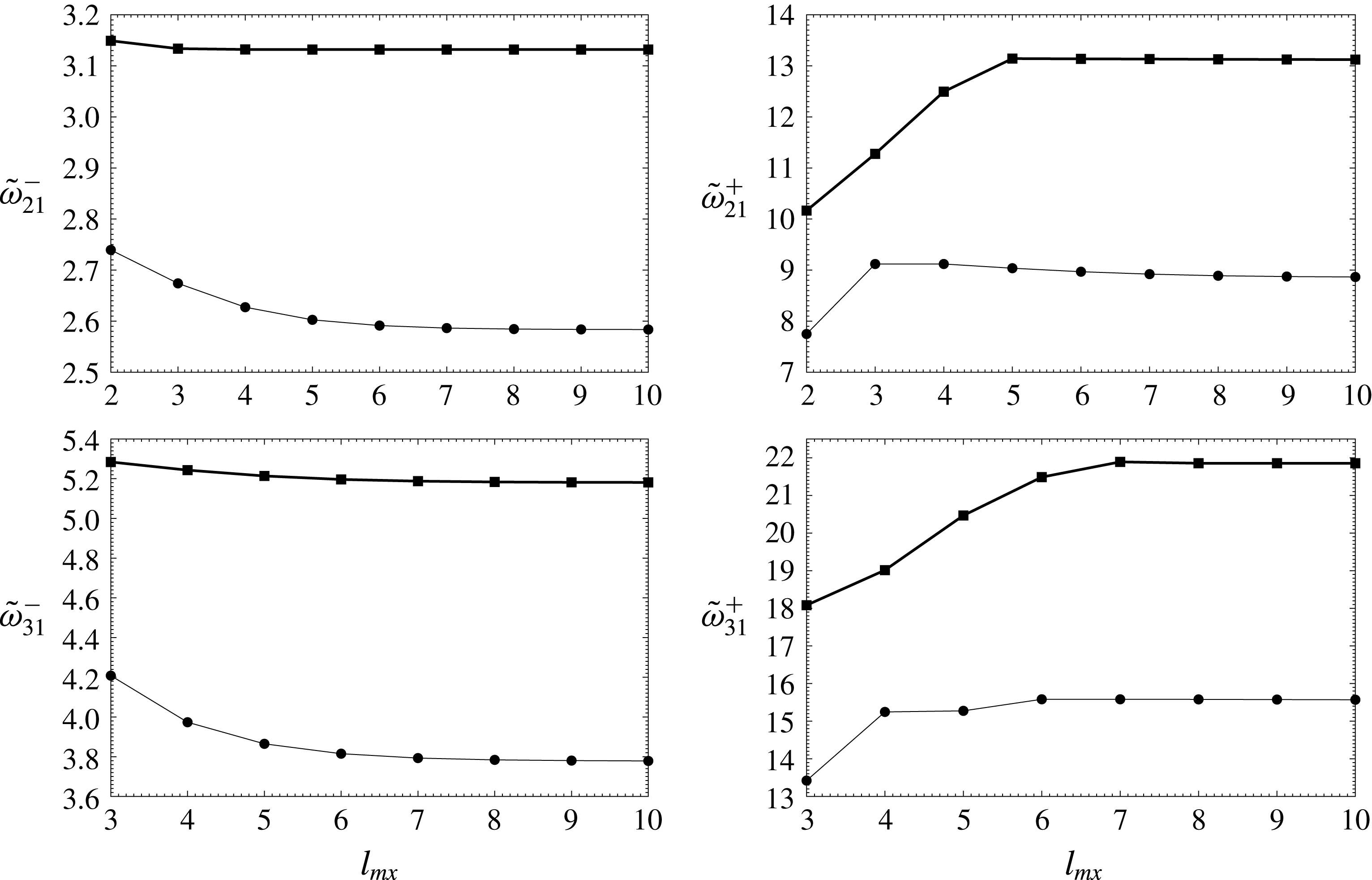
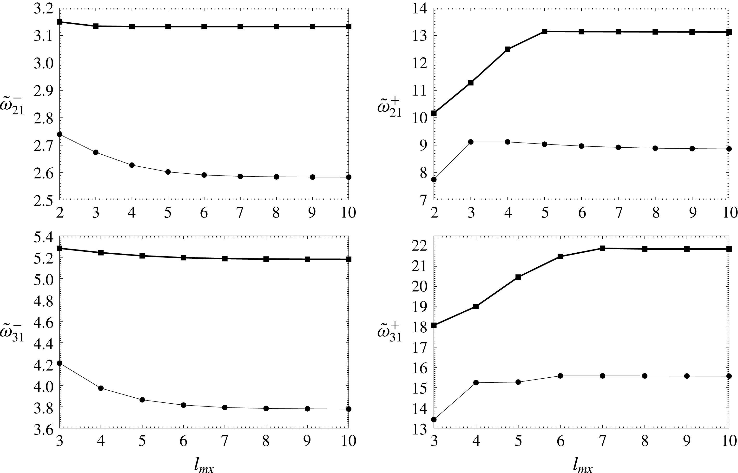
In figure 2, computed values of
 $\tilde{\unicode[STIX]{x1D714}}_{km}^{\pm }$
are plotted as functions of
 $l_{mx}$
for a non-axisymmetric perturbation represented by
 $m=1$
. We also choose two geometric configurations with different size and position of the bubble. In both, we try to ensure close proximity between two interfaces, as this potentially causes slower spectral convergence. Even then, the curves show a fast saturation of computed results for all cases when
 $l_{mx}\geqslant 7$
. The figure also reveals slower saturation of
 $(-)$
modes for larger bubbles, as solutions with higher
 $l$
are needed to properly represent the misaligned waves at two closely located but eccentrically placed interfaces. Conversely,
 $(+)$
modes converge relatively later for a smaller cavity because its deflation normal to the surface makes the peripheral variations more difficult capture by basis functions.
Computed values of normalized natural frequencies for
 $k=2,3$
and
 $m=1$
are plotted as functions of spectral truncation order
 $l_{mx}$
for two geometric configurations with (1)
 $R=0.4a_{0}$
and
 $a_{1}=0.5a_{0}$
(thick line), as well as (2)
 $R=0.25a_{0}$
and
 $a_{1}=0.7a_{0}$
(thin line).
2.4 Parametric study of natural frequency revealing fine-structure split
For a concentric position of the bubble with
 $R=0$
, matrices
 $[M]$
,
 $[S]$
and
 $[P]$
do not have any dependence on the quantum number
 $m$
. This happens because the dynamic equation for a spherically symmetric unperturbed geometry should not have any systemic azimuthal variation. Consequently, a number of vibrational modes with different
 $m$
exhibit the exact same natural frequency when the centres of the drop and the cavity coincide. We refer to this phenomenon as azimuthal degeneracy.
For an eccentrically placed bubble, however, the azimuthal degeneracy disappears, because
 $[M]$
,
 $[S]$
and
 $[P]$
depend on
 $m$
when
 $R\neq 0$
. As a result, one can see small variations in natural frequencies
 $\unicode[STIX]{x1D714}_{km}^{\pm }$
for the modes with different
 $m$
but same
 $k$
. This is the fine-structure split in the wave spectra similar to the one seen in atomic physics, where small changes in energy level occur for different states with different quantum numbers.
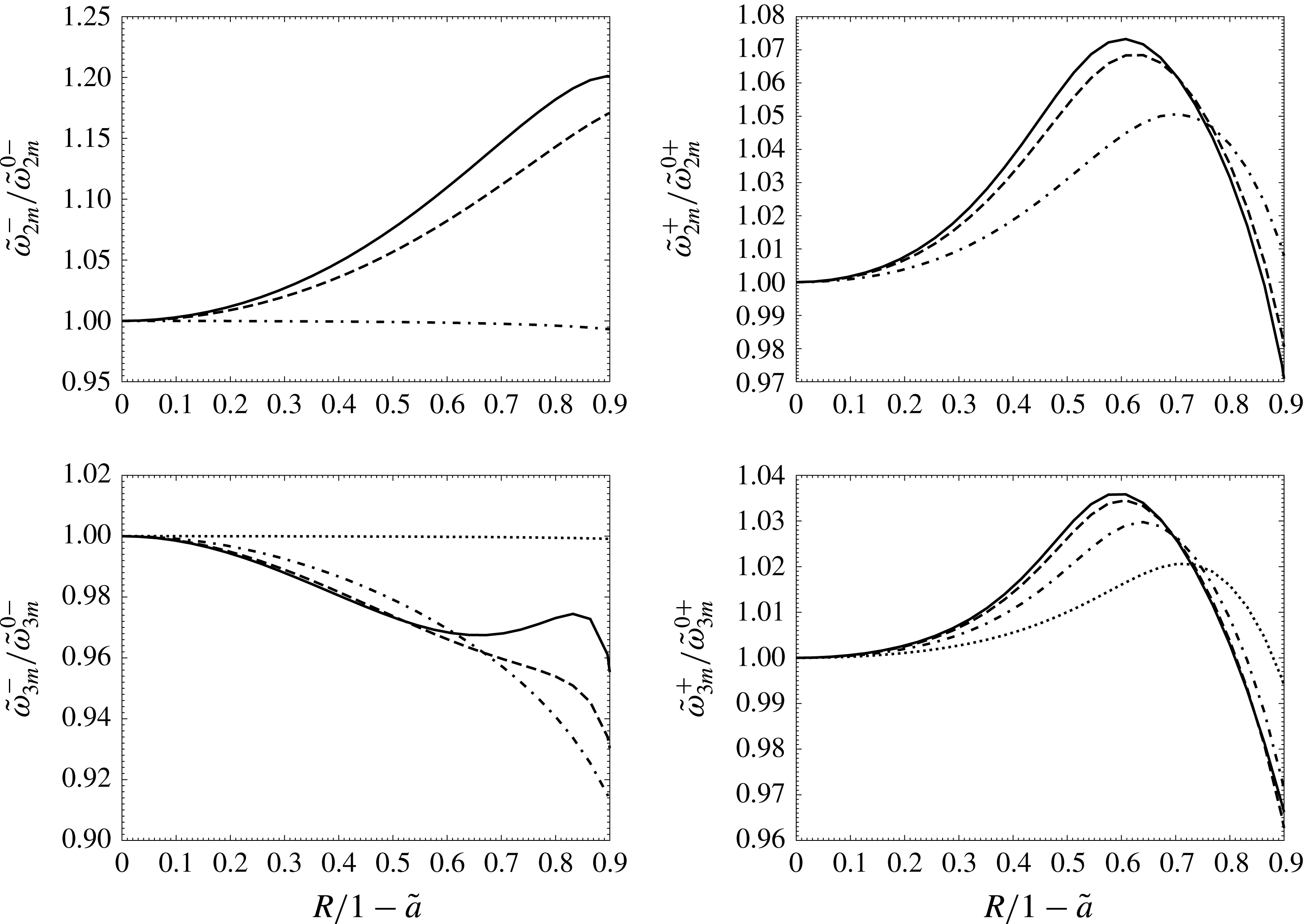
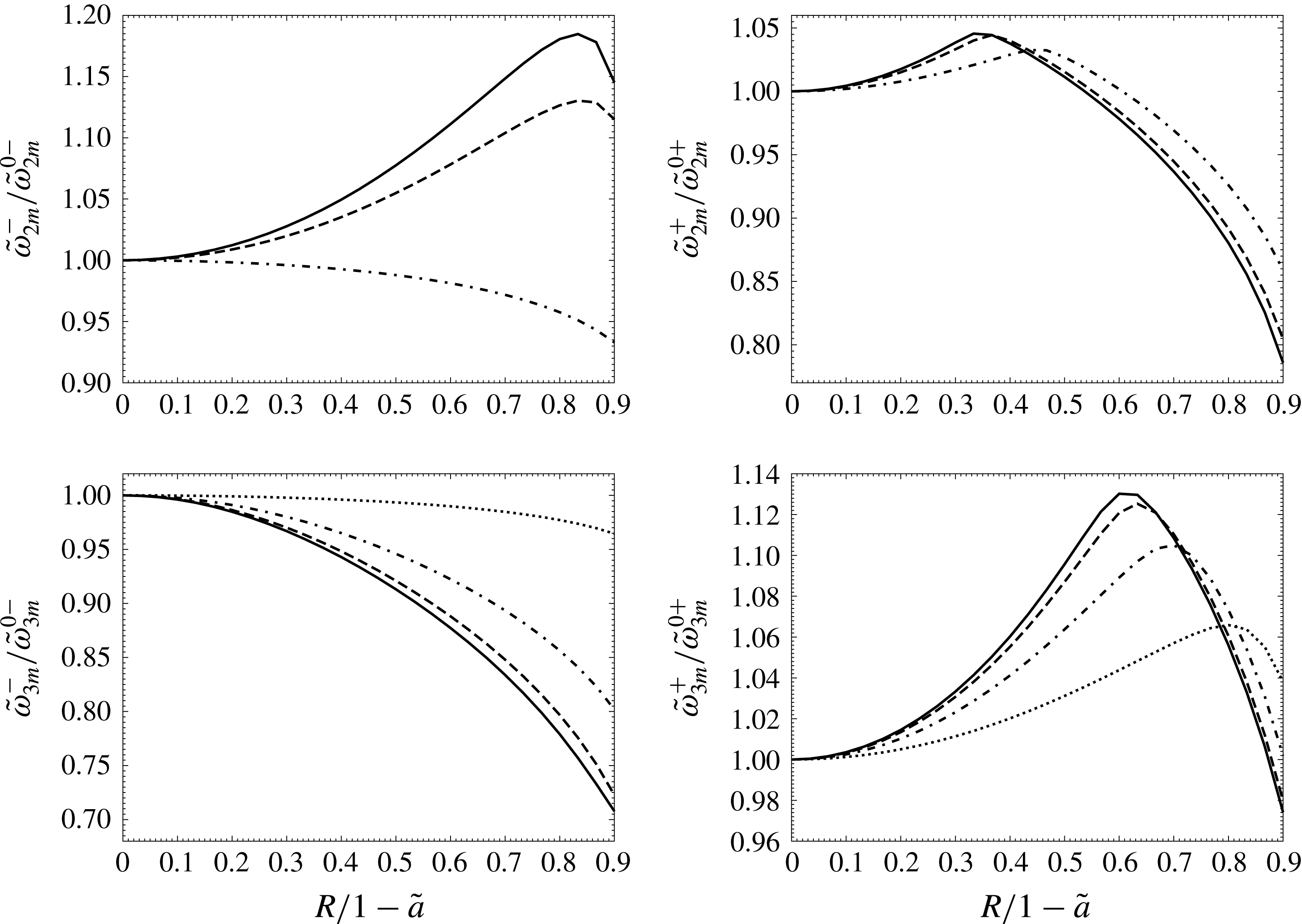
In figures 3 and 4, we illustrate the aforementioned fine-structure split in the frequency spectra for two different size ratios
 $\tilde{a}$
. For all computations,
 $l_{mx}$
is considered as
 $15$
, so that convergence in connection to spectral truncation is not an issue. In each panel, a specific
 $k$
is chosen, and different
 $\unicode[STIX]{x1D714}_{km}^{+}$
or
 $\unicode[STIX]{x1D714}_{km}^{-}$
are plotted as functions of normalized
 $R$
for different
 $m$
values. For concentric position,
 $k$
matches exactly with the quantum number
 $l$
. Hence, for each
 $k$
, we expect
 $(2k+1)$
number of modes with different
 $m$
as it can take the values
 $0,\pm 1,\pm 2,\ldots ,\pm k$
. Among these possible
 $m$
values, however, modes with
 $+m$
and
 $-m$
have the exact same frequency and exact same contour of the deformed interface – these are only separated by a temporal phase. Hence, for each
 $k$
, one can find
 $k+1$
number of fine deviations in frequencies for different
 $m$
values. This dictates the number of curves for respective
 $k$
values in figures 3 and 4.
Normalized natural frequencies for
 $l=2$
and
 $l=3$
as well as plus and minus configurational modes are plotted as functions of position of the bubble normalized by its maximum possible value when the size ratio
 $\tilde{a}=0.5$
and
 $m=0$
(solid line),
 $m=1$
(dashed line),
 $m=2$
(dash-dotted line) and
 $m=3$
(dotted line).

Same as figure 3 with size ratio
 $\tilde{a}$
is
 $0.7$
instead of
 $0.5$
.

To highlight the fine-structure split,
 $\tilde{\unicode[STIX]{x1D714}}_{km}^{\pm }$
are divided by their values
 $\tilde{\unicode[STIX]{x1D714}}_{km}^{0\pm }$
for concentric position at
 $R=0$
. The normalizing factor
 $\tilde{\unicode[STIX]{x1D714}}_{km}^{0\pm }$
is well described in our recently published paper (Bhattacharya Reference Bhattacharya2016) and corroborated in an earlier paper (Tsamopoulos & Brown Reference Tsamopoulos and Brown1987). For example, we find
 $\tilde{\unicode[STIX]{x1D714}}_{2m}^{0-}$
to be
 $2.74$
and
 $2.29$
for
 $\tilde{a}=0.5$
and
 $\tilde{a}=0.7$
. Similarly, our calculations show
 $\tilde{\unicode[STIX]{x1D714}}_{2m}^{0+}$
to be
 $10.11$
and
 $7.32$
for similar size ratios. These values match exactly with the ones reported in Tsamopoulos & Brown (Reference Tsamopoulos and Brown1987). In figures 3 and 4, we use these quantities to renormalize the presented curves which start from
 $1$
. Then, a gradual departure for different
 $m$
values with increasing
 $R$
can be seen in the plots. For small departure from the spherically symmetric geometry, the frequencies should vary as parabolic functions of
 $R$
. This fact is evident in figures 3 and 4. We analyse this behaviour in more detail in a perturbation analysis presented in § 3, where the general numerical simulation is independently corroborated. Also, we consult the results from the aforementioned earlier work focusing on a concentric geometry to check whether the new findings match exactly with the known values when
 $R\rightarrow 0$
.
When
 $R$
approaches
 $a_{0}-a_{1}$
, two interfaces nearly touch each other at the location of minimum separation. It should be noted that touching surfaces lead to the rupture of the film (Patzer & Homsy Reference Patzer and Homsy1975), and the entire analysis is no longer valid from physical considerations. Still, we want to investigate this situation from a purely mathematical perspective. For closely situated interfaces, it is well known that methods based on basis function expansions typically have issues with spectral convergence (Bhattacharya et al.
Reference Bhattacharya, Mishra and Bhattacharya2010; Navardi & Bhattacharya Reference Navardi and Bhattacharya2013). In Stokesian dynamics (Bhattacharya Reference Bhattacharya2008; Navardi & Bhattacharya Reference Navardi and Bhattacharya2010a
,Reference Navardi and Bhattacharya
b
,Reference Navardi and Bhattacharya
c
), this problem is addressed by lubrication analysis, where the predominance of the contributions to hydrodynamic stress from the contact region is presumed. In the present problem, however, the frequency of oscillation is not dictated by the lubrication flow due to its negligible inertia. As a result, one cannot provide a quantitative explanation for spectral behaviour in such a situation. Despite this difficulty, the perturbation analysis in § 3 can qualitatively show why the frequency should vary linearly from a fixed value when
 $R\rightarrow (a_{0}-a_{1})$
.
The frequencies for different
 $m$
but the same
 $k$
diverge considerably with increasing
 $R$
. Still, their differences are significantly smaller than the difference between two modes with unequal
 $k$
or different configurational modes
 $(+)$
or
 $(-)$
. Thus, the spectral plot for interfacial waves would show band structures in frequency space with values for the same
 $k$
and configurational modes grouping together in close proximity. The width and location of these bands change with
 $R$
and
 $\tilde{a}$
. Such a realization can lead to an efficient characterization of multiphase drops. In § 4, we outline an algorithm for this purpose.
3 Matrix perturbation analysis for small geometric deviation
In this section, a perturbation theory validates our simulations independently. It is focused on two limiting cases. The first one is the configuration where the interfaces of the bubble and the drop nearly touch each other at the point of minimum separation. Our asymptotic analysis provides a qualitative description of variations in frequencies with the film thickness although absence of a convenient leading-order solution prohibits a closed form exact result. In contrast, the second study shows a quantitative agreement with the simulation for the near concentric geometry with
 $R\rightarrow 0$
. Both qualitative and quantitative corroborations under two different limits reveal correctness of the mathematical treatment and numerical calculations of § 2.
3.1 Expansion of matrices representing small change in bubble position
Our perturbation analysis analytically describes the change in the frequency values for a specific mode due to a small change in the bubble position
 $R$
. This requires an expansion of the relevant eigen value equation involving the matrix
 $[P]$
defined in § 2.2.
Let us assume that the
 $i$
th eigen value
 $\unicode[STIX]{x1D706}_{0}^{(i)}$
for the eigen vector
 $|\!e_{0}^{(i)}\!\rangle$
of
 $[P]$
is known for a specific position of the bubble at
 $R=R_{0}$
. The quantities associated with this specific location are denoted by the subscript
 $0$
, so that
 $[P]$
at
 $R_{0}$
is referred to as
 $[P_{0}]$
which satisfies
 $$\begin{eqnarray}[P_{0}]|\!e_{0}^{(i)}\!\rangle =\unicode[STIX]{x1D706}_{0}^{i} |\!e_{0}^{(i)}\!\rangle .\end{eqnarray}$$
The question is what the change in the eigen value would be if the position of the bubble were perturbed by a short distance
 $\unicode[STIX]{x1D6FF}$
.
In the new position also, one can write the similar eigen value equation
 $$\begin{eqnarray}[P]|\!e^{(i)}\!\rangle =\unicode[STIX]{x1D706}^{i} |\!e^{(i)}\!\rangle ,\end{eqnarray}$$
where the subscript
 $0$
is dropped to indicate the new position. We consider a perturbative expansion of equation (3.2) treating
 $\unicode[STIX]{x1D6FF}$
as a small parameter
 $$\begin{eqnarray}\displaystyle \left.\begin{array}{@{}c@{}}[P]=[P_{0}]+\unicode[STIX]{x1D6FF}[P_{1}]+\unicode[STIX]{x1D6FF}^{2}[P_{2}]\ldots ,\\ |\!e^{(i)}\!\rangle = |\!e_{0}^{(i)}\!\rangle +\unicode[STIX]{x1D6FF}|\!e_{1}^{(i)}\!\rangle +\unicode[STIX]{x1D6FF}^{2} |\!e_{2}^{(i)}\!\rangle \ldots ,\\ \unicode[STIX]{x1D706}^{(i)}=\unicode[STIX]{x1D706}_{0}^{(i)}+\unicode[STIX]{x1D6FF}\unicode[STIX]{x1D706}_{1}^{(i)}+\unicode[STIX]{x1D6FF}^{2}\unicode[STIX]{x1D706}_{2}^{(i)}\ldots ,\end{array}\right\} & & \displaystyle\end{eqnarray}$$
where the subscript
 $k$
represents the
 $k$
th-order term in the respective perturbations.
We insert the expansion given in (3.3) into (3.2) to derive a hierarchy of equations corresponding to different perturbative orders. The leading zeroth-order relation is already given by (3.1). The next order for
 $i=1$
is governed by the following
 $$\begin{eqnarray}[P_{0}-\unicode[STIX]{x1D706}_{0}^{(i)}]|\!e_{1}^{(i)}\!\rangle +[P_{1}]|\!e_{0}^{(i)}\!\rangle =\unicode[STIX]{x1D706}_{1}^{(i)} |\!e_{0}^{(i)}\!\rangle .\end{eqnarray}$$
The row of eigen vectors
 $\langle f_{0}^{(j)} |$
for the matrix
 $P_{0}$
is also the reciprocal basis for the column vectors. Hence,
 $\langle f_{0}^{(j)} |$
satisfies two conditions simultaneously
 $$\begin{eqnarray}\langle f_{0}^{(j)}\! |[P_{0}-\unicode[STIX]{x1D706}_{0}^{(i)}I]=\langle \!0\!|,\quad \text{and}\quad \langle f_{0}^{(i)}\mid e_{0}^{(j)}\rangle =\unicode[STIX]{x1D6FF}_{ij}.\end{eqnarray}$$
We contract equation (3.4) from the left with
 $\langle f_{0}^{(j)}\! |$
. When the properties of
 $\langle f_{0}^{(j)}\! |$
in (3.5) are utilized, the predominant correction in the eigen values can be derived:
 $$\begin{eqnarray}\unicode[STIX]{x1D706}_{1}^{(i)}=\langle f_{0}^{(i)}\! |[P_{1}]\!|\!e_{0}^{(i)}\!\rangle .\end{eqnarray}$$
This is the slope by which the eigen value
 $\unicode[STIX]{x1D706}^{(i)}$
varies with the position of the bubble.
The frequency of the
 $i$
th mode, renamed here as
 $\unicode[STIX]{x1D714}^{(i)}$
instead of
 $\unicode[STIX]{x1D714}_{km}^{\pm }$
, is the square root of
 $\unicode[STIX]{x1D706}^{(i)}$
. Let us now assume
 $R_{0}\rightarrow (a_{0}-a_{1})$
with the two interfaces nearly touching each other. Then, one expects a linear dependence of
 $\unicode[STIX]{x1D714}^{(i)}$
on the thickness
 $h$
of the so called lubrication region around minimum separation. Thus, the variation would be
 $$\begin{eqnarray}\unicode[STIX]{x1D714}^{(i)}=\sqrt{\unicode[STIX]{x1D706}_{0}^{(i)}}+h\unicode[STIX]{x1D6FA}_{1}^{(i)},\end{eqnarray}$$
where the constant
 $\unicode[STIX]{x1D6FA}_{1}^{(i)}$
is given by
 $$\begin{eqnarray}\unicode[STIX]{x1D6FA}_{1}^{(i)}=\left.-\unicode[STIX]{x1D706}_{1}^{(i)}\right/\left(2\sqrt{\unicode[STIX]{x1D706}_{0}^{(i)}}\right).\end{eqnarray}$$
Unfortunately, the leading-order eigen values under touching conditions with
 $h\rightarrow 0$
is not readily available from a simplified mathematical analysis. One has to solve the field equations in the tangent sphere coordinate system so that the corresponding matrix formulation ultimately yields these quantities. However, such a result would not have any physical meaning, as the bubble will simply rupture in such a configuration. This is why we did not pursue a detailed calculation when the two interfaces nearly touch each other. Still, from a purely mathematical perspective, the perturbation analysis provides a qualitative agreement, as all curves in figures 3 and 4 obey the functional form in equation (3.7). This means that the change
 $\unicode[STIX]{x0394}\unicode[STIX]{x1D714}^{(i)}$
in frequency should scale as
 $$\begin{eqnarray}\unicode[STIX]{x0394}\unicode[STIX]{x1D714}^{(i)}\sim \sqrt{h^{2}\unicode[STIX]{x1D6FE}/(\unicode[STIX]{x1D70C}a_{0}^{5})},\end{eqnarray}$$
instead of the scaling
 $\sqrt{\unicode[STIX]{x1D6FE}/(\unicode[STIX]{x1D70C}a_{0}^{3})}$
seen in (2.18).
3.2 Asymptotic results under the limit of nearly concentric geometry
The first-order correction in equation (3.6) should not be enough to explain the leading-order variation of frequencies with
 $R$
for a nearly concentric geometry. The reason is based on the reflectional symmetry in the
 $x$
–
 $y$
plane making
 $\unicode[STIX]{x1D706}_{1}^{(i)}$
equal to zero when
 $R_{0}=0$
. In other words, if the bubble is displaced upward or downward by the same distance with respect to the centre of the drop, the resulting two systems will be essentially identical apart from the configurational orientation. Thus, in both cases, the wave frequencies should be exactly the same, making the eigen value an even function of
 $R$
. This is why we have seen a parabolic dependence of all
 $\unicode[STIX]{x1D714}_{km}^{\pm }$
in figures 3 and 4 for
 $R\rightarrow 0$
. Quantitative description of this variation requires an analysis of the second-order perturbation.
The second-order relation for the eigen value equation is
 $$\begin{eqnarray}[P_{0}-\unicode[STIX]{x1D706}_{0}^{(i)}]\!|\!e_{2}^{(i)}\!\rangle +[P_{1}]\!|\!e_{1}^{(i)}\!\rangle +[P_{2}]\!|\!e_{0}^{(i)}\!\rangle =\unicode[STIX]{x1D706}_{2}^{(i)}\! |\!e_{0}^{(i)}\!\rangle .\end{eqnarray}$$
We contract equation (3.10) from the left with
 $\langle f_{0}^{(i)}\! |$
, and use its properties to find
 $$\begin{eqnarray}\unicode[STIX]{x1D706}_{2}^{(i)}=\langle f_{0}^{(i)}\! |[P_{1}]\!|\!e_{1}^{(i)}\!\rangle +\langle f_{0}^{(i)}\! |[P_{2}]\!|e_{0}^{(i)}\!\rangle .\end{eqnarray}$$
From (3.10), one can conclude
 $$\begin{eqnarray}|\!e_{1}^{(i)}\!\rangle =\unicode[STIX]{x1D706}_{1}^{(i)}[P_{0}-\unicode[STIX]{x1D706}_{0}^{(i)}I]^{BI}\! |\!e_{0}^{(i)}\!\rangle -[P_{0}-\unicode[STIX]{x1D706}_{0}^{(i)}I]^{BI}[P_{1}]\!|e_{0}^{(i)}\!\rangle .\end{eqnarray}$$
Here, the superscript
 $BI$
denotes partial or block inverse of singular matrix
 $[P_{0}-\unicode[STIX]{x1D706}_{0}^{(i)}I]$
with its non-null block being identified and inverted without changing its null space
 $$\begin{eqnarray}[P_{0}-\unicode[STIX]{x1D706}_{0}^{(i)}I]^{BI}=[P_{0}-\unicode[STIX]{x1D706}_{0}^{(i)}I+ |\!e_{0}^{(i)}\!\rangle \langle f_{0}^{(i)}\! |]^{-1}-|\!e_{0}^{(i)}\!\rangle \langle f_{0}^{(i)}\! |.\end{eqnarray}$$
Combining, equations (3.11) and (3.12), the second-order correction in the eigen value is obtained
 $$\begin{eqnarray}\unicode[STIX]{x1D706}_{2}^{(i)}=\langle f_{0}^{(i)}\! |[P_{2}]\!|\!e_{0}^{(i)}\!\rangle -\langle f_{0}^{(i)}\! |[P_{1}][P_{0}-\unicode[STIX]{x1D706}_{0}^{(i)}I]^{BI}[P_{1}]\!|\!e_{0}^{(i)}\!\rangle ,\end{eqnarray}$$
where
 $\unicode[STIX]{x1D706}_{1}^{(i)}=0$
is presumed for
 $R_{0}=0$
.
Fortunately, for
 $R_{0}=0$
, all matrices
 $[P_{0}]$
,
 $[P_{1}]$
,
 $[P_{2}]$
have simple forms. Our analysis first constructs
 $[P_{0}]$
,
 $[P_{1}]$
,
 $[P_{2}]$
in terms of the perturbation terms in the mass matrix
 $[M]$
and spring matrix
 $[S]$
. Accordingly, the expansions for
 $[M]$
and
 $[S]$
are defined
 $$\begin{eqnarray}[M]=[M_{0}]+\unicode[STIX]{x1D6FF}[M_{1}]+\unicode[STIX]{x1D6FF}^{2}[M_{2}]\ldots ,\quad [S]=[S_{0}]+\unicode[STIX]{x1D6FF}[S_{1}]+\unicode[STIX]{x1D6FF}^{2}[S_{2}]\ldots ,\end{eqnarray}$$
and the
 $i$
th-order contributions
 $[M_{i}]$
and
 $[S_{i}]$
are explicitly determined using the
 $R$
-dependent expression of the respective matrices. The explicit forms of the
 $i$
th-order terms are given below
 $$\begin{eqnarray}[M_{0}]=\left[\begin{array}{@{}cc@{}}[I] & [T_{0}^{f}]\\ \hspace{0.0pt}[T_{0}^{r}] & [I]\end{array}\right],\quad [S_{0}]=\left[\begin{array}{@{}cc@{}}[D^{0}] & -[\tilde{T}_{0}^{f}]\\ -[\tilde{T}_{0}^{r}] & [D^{1}]\end{array}\right],\end{eqnarray}$$
and for
 $i>0$
 $$\begin{eqnarray}[M_{i}]=\left[\begin{array}{@{}cc@{}}[0] & [T_{i}^{f}]\\ \hspace{0.0pt}[T_{i}^{r}] & [0]\end{array}\right],\quad [S_{i}]=\left[\begin{array}{@{}cc@{}}[0] & -[\tilde{T}_{i}^{f}]\\ -[\tilde{T}_{i}^{r}] & [0]\end{array}\right].\end{eqnarray}$$
Here, the components of the off-diagonal blocks of
 $[M_{i}]$
are only non-zero when
 $l=l^{\prime }+i$
for which
 $$\begin{eqnarray}T_{i}^{r}(l^{\prime },l)=\frac{\tilde{a}^{l^{\prime }}}{(l-l^{\prime })!}\sqrt{\frac{(2l+1)(l-m)!(l+m)!}{(2l^{\prime }+1)(l^{\prime }-m)!(l^{\prime }+1)!}},\quad \text{and}\quad T_{i}^{f}(l,l^{\prime })=\tilde{a}T_{i}^{r}(l^{\prime },l).\end{eqnarray}$$
Similarly, only non-zero elements in the off-diagonal blocks of
 $[S_{i}]$
can be evaluated by relating them to
 $[M_{i}]$
 $$\begin{eqnarray}\tilde{T}_{i}^{r}(l,l^{\prime })=\tilde{a}^{-3}l(l^{2}+l-2)T_{i}^{r}(l,l^{\prime })\quad \text{and}\quad \tilde{T}_{i}^{f}(l,l^{\prime })=\tilde{a}(l+1)(l^{2}+l-2)T_{i}^{r}(l^{\prime },l).\end{eqnarray}$$
In contrast, the diagonal blocks of the matrices are either the identity matrix
 $[I]$
or the null matrix
 $[0]$
or the matrices defined in (2.14).
For our problem,
 $[P]$
is the product of the inverse of
 $[M]$
and
 $[S]$
. This definition yields:
 $$\begin{eqnarray}\displaystyle & \displaystyle [P_{0}]=[M_{0}]^{-1}[S_{0}], & \displaystyle\end{eqnarray}$$
 $$\begin{eqnarray}\displaystyle & \displaystyle [P_{1}]=[M_{0}]^{-1}[S_{1}]-[M_{0}]^{-1}[M_{1}][M_{0}]^{-1}[S_{0}], & \displaystyle\end{eqnarray}$$
 $$\begin{eqnarray}\displaystyle & \displaystyle [P_{2}]=[M_{0}]^{-1}\{[S_{2}]-[M_{1}][M_{0}]^{-1}([S_{1}]-[M_{1}][M_{0}]^{-1}[S_{0}])-[M_{2}][M_{0}]^{-1}[S_{0}]\}.\quad & \displaystyle\end{eqnarray}$$
For
 $R_{0}=0$
, we checked that the specific forms of
 $\langle f_{0}^{(i)}\! |$
,
 $[P_{1}]$
and
 $|\!e_{0}^{(i)}\!\rangle$
make
 $\unicode[STIX]{x1D706}_{1}^{(i)}=0$
according to (3.6). Consequently,
 $\unicode[STIX]{x1D706}_{2}^{(i)}$
contributes as the most prominent correction. Then, we can express the non-dimensional frequency in the following form
 $$\begin{eqnarray}\tilde{\unicode[STIX]{x1D714}}_{km}^{\pm }=\tilde{\unicode[STIX]{x1D714}}_{km}^{0\pm }+\tilde{\unicode[STIX]{x1D6FA}}_{km}^{\pm }(\tilde{a})R^{2}/a_{0}^{2},\end{eqnarray}$$
where the dimensionless parameter
 $\tilde{\unicode[STIX]{x1D6FA}}_{km}^{\pm }$
represents the quadratic behaviour in
 $R$
 $$\begin{eqnarray}\tilde{\unicode[STIX]{x1D6FA}}^{(i)}=\sqrt{\frac{\unicode[STIX]{x1D70C}a_{0}^{3}}{\unicode[STIX]{x1D6FE}}}\frac{a_{0}^{2}\unicode[STIX]{x1D706}_{2}^{(i)}}{\sqrt{4\unicode[STIX]{x1D706}_{0}^{(i)}}}.\end{eqnarray}$$
Here, the superscript
 $(i)$
is interchangeably used in place of quantum numbers.
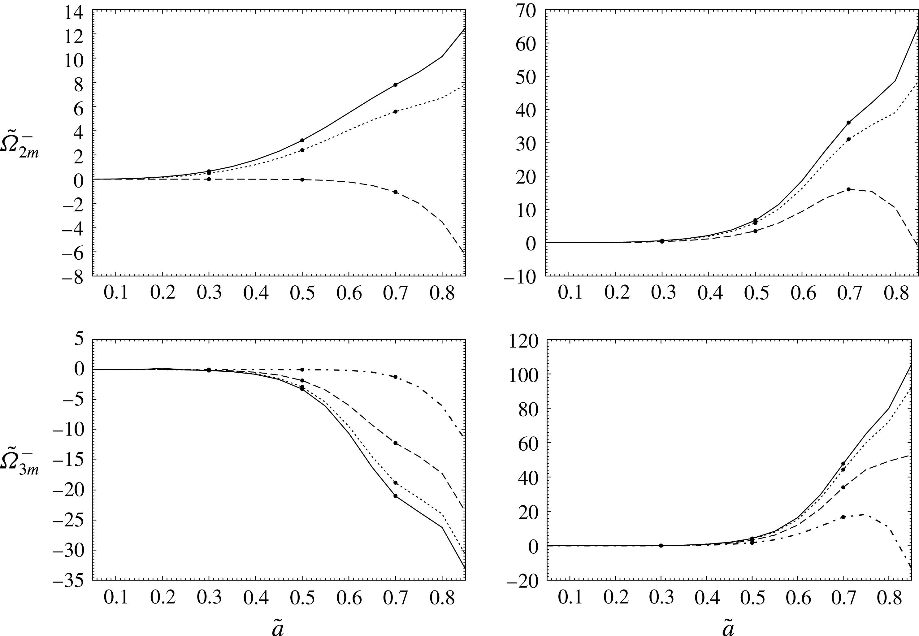
The parameter
 $\tilde{\unicode[STIX]{x1D6FA}}_{lm}$
computed from (3.24) according to perturbation theory is plotted as a function of
 $\tilde{a}$
for plus and minus spectral modes as well as
 $l=2$
and
 $l=3$
, when
 $m=0$
(solid line),
 $m=1$
(dotted line),
 $m=2$
(dashed line) and
 $m=3$
(dash-dotted line). The results from the general simulation presented in § 2 are shown as large dotted points for a few selected size ratios.

In figure 5, we present the calculated
 $\tilde{\unicode[STIX]{x1D6FA}}_{km}^{\pm }$
according to the perturbation analysis as a function of the size ratio. The results from the asymptotic theory are presented as the line curves for different quantum numbers. In contrast, the corresponding values from the general simulation, discussed in § 2, are shown as isolated data points for a few specific
 $\tilde{a}$
. The latter match exactly with the former, establishing an important corroboration between the two independent approaches, validating both.
4 Detection of a bubble in an opaque drop from interfacial spectra
An interesting application of the outlined theory would be a non-invasive detection technique which can characterize an embedded bubble inside a suspended opaque drop whose interior is not visible from the outside. The procedure would exploit the observable spectral features of the system exhibited in its natural pulsation in suspended condition. Then, the experimentally determined frequencies can be matched with the simulated estimations to predict the size and position of the internal cavity. The method can also be extended for a particle-laden droplet.
The validity of the outlined procedure can be ensured only for small-amplitude oscillations under a low capillary number limit. Despite these constraints, we expect this to be viable for a wide range of applications, because exact similar assumptions have not limited the experimental and technological relevance of Rayleigh’s theory (Rayleigh Reference Rayleigh1879).
The aforementioned non-intrusive detection method requires both experimental determination and theoretical predictions of the natural frequencies. Then, two sets of results can be compared in a pattern recognition algorithm to extract the desired parameters of interest. There are two prerequisites for the scheme to work. Firstly, the bubble–drop system has to be in under-damped condition so that it undergoes spontaneous natural pulsation. This criterion is assured if the capillary number is small. Secondly, we need an optical device like a high-speed camera to record the interfacial displacements as functions of time and peripheral positions in a non-invasive way. Advancement of modern technology provides such equipment so that the data can be stored with the necessary details making experimental determination of spectral quantities possible. In this section, we describe the essential elements of the characterization process.
4.1 Outline of the detection and characterization algorithm
The detection method would require three major steps. Firstly, the interfacial pulsation has to be recorded in an experiment (Saffren, Elleman & Rhim Reference Saffren, Elleman and Rhim1982). Secondly, the relevant spectral quantities have to be evaluated from the stored data. Finally, the convenient features of experimentally obtained values should be properly matched with the theoretical prediction of a possible system by an efficient algorithm.
The first two steps are conceptually straightforward. One can use a high-speed camera to view the pulsation of the drop. As a result, its radial deformation
 $s^{ex}$
at the outer surface can be recorded as a series of two-dimensional images taken at subsequent time intervals. The observed displacement from the average contour has to be stored as a function of time and polar coordinate
 $\unicode[STIX]{x1D6FD}$
on the viewing plane. Then, the frequency spectra of the interfacial dynamics can be experimentally determined by a dual Fourier transform
 $C_{\unicode[STIX]{x1D708}}(\unicode[STIX]{x1D714})$
 $$\begin{eqnarray}C_{\unicode[STIX]{x1D708}}(\unicode[STIX]{x1D714})=\int s^{ex}(t,\unicode[STIX]{x1D6FD})\text{e}^{\text{i}\unicode[STIX]{x1D708}\unicode[STIX]{x1D6FD}}\text{e}^{\text{i}\unicode[STIX]{x1D714}t}\,\text{d}\unicode[STIX]{x1D6FD}\,\text{d}t.\end{eqnarray}$$
Complete spectral description of the system requires
 $C_{\unicode[STIX]{x1D708}}$
to be evaluated for
 $\unicode[STIX]{x1D708}=0,1,2,\ldots$
, as natural frequencies for all
 $l$
values would be revealed by
 $C_{\unicode[STIX]{x1D708}}(\unicode[STIX]{x1D714})$
. Consequently, spectral plots of
 $C_{\unicode[STIX]{x1D708}}$
in the frequency domain will show several spikes grouped together in bands according to our theory of fine-structure split.
This spectral manifestation can be used to predict the volume fraction
 $\unicode[STIX]{x1D719}$
and position
 $R$
of the cavity inside the drop by matching the observation with the theoretical predictions. For this purpose, an efficient algorithm can be built after identifying useful features of the variation of frequency values for different modes in parametric space. The strategy would be to recognize quantities which only vary with one system parameter while showing negligible dependence on others. From the spectral results in § 2, we identify such signature features which are discussed in the subsequent subsections.
4.2 Convenient features of fine spectral structure indicating the volume fraction
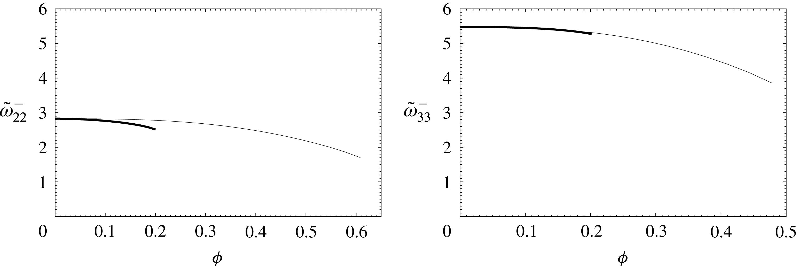
Computed
 $\tilde{\unicode[STIX]{x1D714}}_{kk}^{-}$
are plotted as functions of volume fraction with
 $R/a_{0}=0.2$
(thin line) and
 $R/a_{0}=0.4,0.6,0.8$
(thick line) for
 $k=2,3$
.

The efficient characterization algorithm requires recognition of spectral features which only varies with either of position
 $R$
or volume fraction
 $\unicode[STIX]{x1D719}=\tilde{a}^{3}$
. Such quantities are readily available in the plots presented in § 2.4. One can see that the frequencies for the
 $(-)$
modes corresponding to
 $k=|m|$
have negligible variation with
 $R$
. This is especially true for higher values of
 $l$
. The slow dependence in the fields along
 $z$
-direction for
 $k=m$
is the reason behind the observed behaviour. Thus, one can identify
 $\unicode[STIX]{x1D714}_{kk}^{-}$
to be a signature variable which should be conveniently used to find the volume fraction
 $\unicode[STIX]{x1D719}$
.
The approximate invariance of
 $\unicode[STIX]{x1D714}_{kk}^{-}$
with
 $R$
is further revealed in figure 6. We choose four different values of
 $R$
and present the non-dimensional
 $\tilde{\unicode[STIX]{x1D714}}_{22}^{-}$
and
 $\tilde{\unicode[STIX]{x1D714}}_{33}^{-}$
as functions of volume fraction of the cavity. The curves in the figures are of different lengths because allowable volume fractions are limited for an eccentrically situated bubble. For
 $k=m=2$
, three of these curves merge with each other altogether. For
 $k=m=3$
, the invariance with
 $R$
is even more prominent – there, all four curves collapse onto each other showing no change whatsoever for variation in
 $R$
.
This implies that
 $\tilde{\unicode[STIX]{x1D714}}_{33}^{-}$
can be treated as a signature parameter which solely depends on
 $\unicode[STIX]{x1D719}$
. So if this variation is tabulated properly, one can predict the volume fraction from the observed value of the
 $\tilde{\unicode[STIX]{x1D714}}_{33}^{-}$
.
However, in order to characterize the bubble,
 $\tilde{\unicode[STIX]{x1D714}}_{33}^{-}$
has to be located in the experimentally observed spectral data. The second band in the spectral plot corresponds to the
 $k=3$
and
 $(-)$
configurational mode. The last peak in that cluster represents the frequency value for
 $m=k=3$
. Thus, if one locates this quantity in the experimental data acquired following the procedure in § 4.1, the volume fraction for the cavity can be detected.
4.3 Detection of bubble position from bandwidth
Once the volume fraction is known, it is easy to find the position of the bubble from various other quantities. Among all others, the most reliable and convenient parameter could be the width
 $\unicode[STIX]{x1D6FF}\unicode[STIX]{x1D714}_{k}^{\pm }$
of the first few prominent bands. This quantity is the interval in the spectral space in which the fine-structure split ensures a number of modes for the same specific
 $l$
to be clustered together. One can evaluate the width of this band from the difference between the maximum and minimum of closely situated frequencies for different
 $m$
but the same
 $l$
.
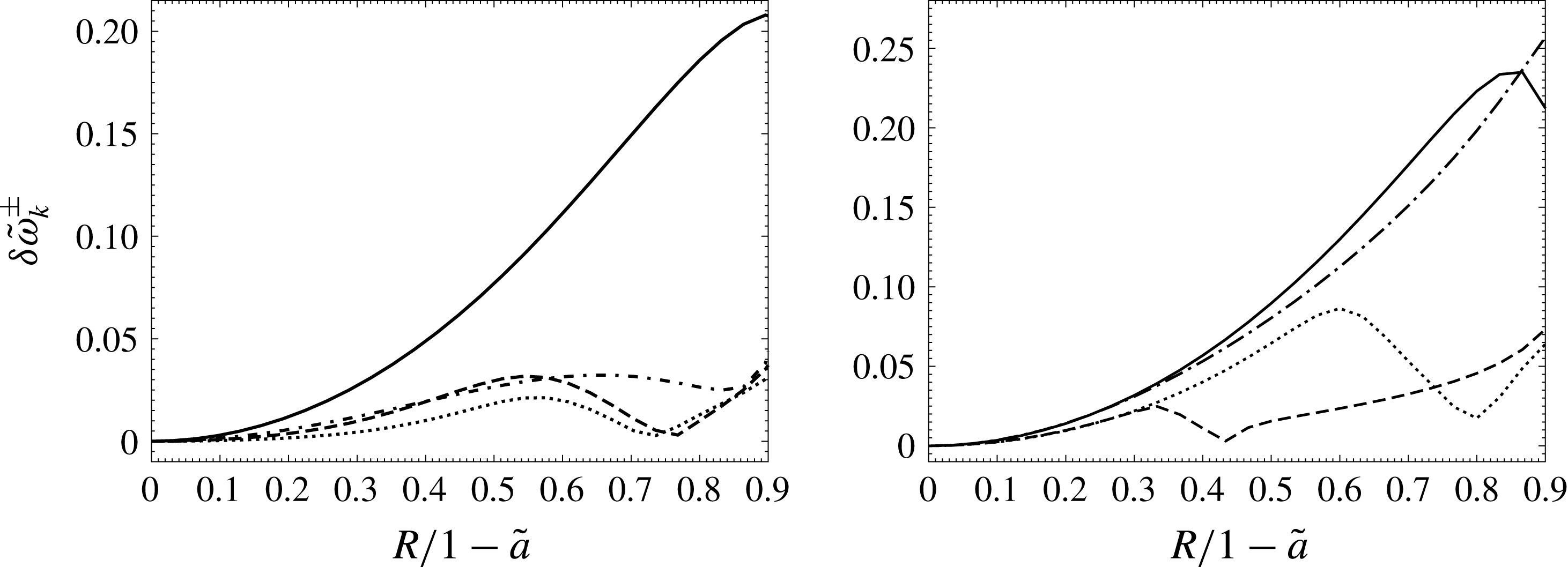
In figure 7, we present bandwidths for four most relevant modes as functions of the normalized position of the bubble for two different volume fractions. The plots show non-trivial variation in
 $\unicode[STIX]{x1D6FF}\unicode[STIX]{x1D714}_{k}^{\pm }$
with
 $R$
.
Bandwidths of non-dimensional frequency are plotted as functions of normalized position for
 $(-)$
configurational modes with
 $k=2$
(solid line) and
 $k=3$
(dash-dot line) as well as
 $(+)$
configurational modes with
 $k=2$
(dashed line) and
 $k=3$
(dotted line), where the size ratio is
 $\tilde{a}=0.5$
(left) and
 $\tilde{a}=0.7$
(right).

The bands for specific
 $k$
can be identified in the experimentally acquired spectral data by the number of fine structures in that group. This number should be exactly the same as
 $k+1$
. Also, there would be two bands with same number of fine structures. Between these two, the one with the lower value represents the
 $(-)$
configurational mode, whereas the
 $(+)$
mode corresponds to the larger number. In this way it is possible to locate
 $\unicode[STIX]{x1D6FF}\unicode[STIX]{x1D714}_{k}^{\pm }$
in the observed frequency spectra.
These quantities can reveal the position of the bubble in the following way. Firstly, the theory outlined in § 2 can be used to compute the bandwidth as a function of
 $R$
for the known value of the already detected volume fraction. Then, an error
 $\unicode[STIX]{x1D716}$
can be defined as
 $$\begin{eqnarray}\unicode[STIX]{x1D716}=\mathop{\sum }_{k}(\unicode[STIX]{x1D6FF}\unicode[STIX]{x1D714}_{k}^{+}-\unicode[STIX]{x1D6FF}\unicode[STIX]{x1D714}_{k}^{ex+})^{2}+\mathop{\sum }_{k}(\unicode[STIX]{x1D6FF}\unicode[STIX]{x1D714}_{k}^{-}-\unicode[STIX]{x1D6FF}\unicode[STIX]{x1D714}_{k}^{ex-})^{2},\end{eqnarray}$$
where superscript ‘
 $ex$
’ describes the experimentally observed bandwidth. One can choose a few representative
 $k$
so that
 $\unicode[STIX]{x1D716}$
relates to a mean square departure in the simulated result from the experimental values. In the end, an error versus position plot can indicate the location of the cavity by presuming that it corresponds to the minimum
 $\unicode[STIX]{x1D716}$
.
It is to be noted that the position of the bubble may change in time due to various reasons. Firstly, it can move due to the presence of an external potential such gravity. In that case, a low Bond number limit would ensure a very slow temporal change in
 $R$
. Secondly, the system itself might be unstable, causing departure due to nonlinear shape oscillation (Shaw Reference Shaw2006). However, the time required for such translation is always much larger than the temporal scale dictated by the interfacial frequencies (Tsamopoulos & Brown Reference Tsamopoulos and Brown1987). Thus, for either case, one can apply a multiple time scale analysis to describe the complex dynamics. In such a formulation, the leading-order spectra for nominal fluctuations would be similar to our findings. Then, additionally, the natural frequencies would also alter slowly over a longer period where this slow evolution can indicate the translational dynamics inside the liquid domain.
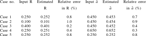
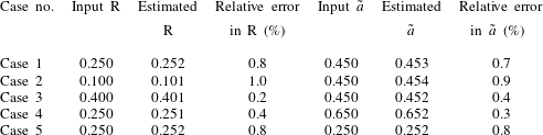
The comparison between the values of the system parameters used as inputs for the dynamic evolution and the estimations of the same quantities obtained from the detection algorithm.
We perform a numerical experiment to confirm the viability of the described detection technique. Accordingly, a bubble–drop system is considered where an input configuration with specific
 $\tilde{a}$
and
 $R$
values is assigned. Then, it is assumed that
 $126$
different modes corresponding to
 $k$
values varying from
 $2$
to
 $10$
are involved in the interfacial pulsation. These include waves with different
 $m=0,1,\ldots ,k$
and configurational orientations
 $+$
and
 $-$
for each
 $k$
. The non-dimensional amplitudes for each of the modes are randomly generated numbers between
 $0.01$
and
 $0.05$
. Once these random values are fixed, the deformation at the outer surface is calculated using the field solutions equation (2.4) given in § 2.1. Consequently, the projection of the instantaneous image of the deforming drop is computed taking the
 $y$
–
 $z$
surface to be the two-dimensional viewing plane. The radial deviation
 $s^{ex}$
of the image is recorded as a function of time and the polar angle on the viewing plane. Next, the spectral response
 $C_{\unicode[STIX]{x1D708}}$
is calculated using the dual Fourier transform in (4.1), revealing the natural frequencies of the system as the resulting peaks in the spectral space. Finally,
 $\tilde{a}$
and
 $R$
are estimated from these data by exploiting known features of
 $\tilde{\unicode[STIX]{x1D714}}_{33}^{-}$
as well as minimizing the errors according to (4.2) in the observed and computed bandwidths.
The estimated and the input values of
 $\tilde{a}$
and
 $R$
are presented in table 1. We select
 $5$
different systems for our case study so that it covers the possible parametric space properly. Accordingly, the first simulation has moderate
 $R$
and
 $\tilde{a}$
identified as
 $0.25$
and
 $0.45$
, respectively. Then, we choose two extreme values for
 $R$
as
 $0.1$
and
 $0.4$
representing a slightly eccentric bubble and one nearly touching the external surface. Similarly, two additional
 $\tilde{a}$
values are also accounted for to evaluate the effectiveness of our scheme for both small and large cavities. The extreme values of one parameter are taken into account keeping the other parameter moderate so that ultimately
 $5$
different configurations can include all possible situations.
The results for the numerical experiment show the correctness of the detection algorithm. A majority of the case studies show less than
 $1\,\%$
relative error between the actual input and the estimated prediction. The error is lower for larger bubbles and for more eccentric locations. This is understandable because such configurations enhance the interactions between the interfaces, leading to a more accurate detection due to more prominent surface dynamics. The comparative exploration is a necessary consistency test inferring the outlined diagnostic technique to be robust and implementable as long as the caveats of our analysis are satisfied and experiments are accurate enough.
5 Summary and concluding remarks
This article reveals the details of the frequency spectra for interfacial pulsation of a drop with an embedded bubble in an arbitrary position. The different waves in the system are represented by two quantum numbers
 $k=1,2,3\ldots$
and
 $m=0,\pm 1,\pm 2,\ldots ,\pm l$
as well as by two configurational modes
 $(-)$
and
 $(+)$
. The results show that there can be small deviations in frequencies for modes with different
 $m$
when
 $k$
is the same. We refer to this phenomenon as fine-structure split which is analogous to the one seen in atomic systems with small variations in energy level due to different quantum numbers.
The fine-structure split only appears when the cavity is in an eccentric position with respect to the droplet. For a concentric geometry, these small deviations in frequency disappear, because in that case these values coincide for modes with different
 $m$
but the same
 $k$
. Such a coincidence, termed azimuthal degeneracy, occurs due to the azimuthal invariance of the governing equation and spherical symmetry of the geometry.
When the bubble is displaced from the spherically symmetric position, fine spectral structures appear. As a result, one can see different closely situated frequencies forming bands together in the spectral domain.
We compute these frequencies by expanding the flow field in basis functions. Then, a system of algebraic equations is represented in a matrix form by exploiting the homogeneous boundary conditions dictated by surface tension at the interfaces. The frequencies of different modes are related to the eigen values of the involved matrix. In case of a concentric system, the relations are block diagonalized in
 $k$
and degenerated in
 $m$
causing the azimuthal degeneracy. In contrast, for an eccentrically placed cavity, the modes with different
 $k$
are coupled, leading to only block diagonalization in
 $m$
. Thus, if
 $m$
is changed, the same
 $k$
yields a slightly modified frequency.
The distinct effect of the eccentrically placed cavity in the form of band structure creation allows us to conceptualize a possible detection method. The procedure would exploit the processed spectral data from experimentally observed droplet pulsations to characterize the size and position of the bubble. For this purpose, we identify signature variables which only vary with one system defining parameter while the others remain invariant. One such signature is the frequency
 $\unicode[STIX]{x1D714}_{33}^{-}$
which varies only with volume fraction
 $\unicode[STIX]{x1D719}$
and exhibits negligible change with position
 $R$
. This mode can be easily located in the spectral plot as the last peak of the fine structures of the second band in frequency space. Thus,
 $\unicode[STIX]{x1D719}$
can be determined from the observed
 $\unicode[STIX]{x1D714}_{33}^{-}$
. Then,
 $R$
can also be estimated by matching the simulated bandwidths for the predicted size ratio to the observed values.
We also validate our general simulation with a novel matrix perturbation theory under limiting situations. The analysis shows a very precise quantitative agreement between two sets of results when the bubble is slightly displaced from its concentric position. Also, the comparison implies a qualitative verification of our numerical results for a nearly touching configuration of the two interfaces.
The fine-structure split can also be observed for an embedded particle instead of a bubble. Moreover, the same phenomenon can be used to characterize a system with multiple gaseous cavities and solid bodies inside the liquid domain. In the near future, we intend to generalize our analysis so that these more complex dynamics can be described.
The analysis can be extended to different geometries also. For example, we can consider an elliptical drop instead of a spherical one. In that case, one should use solutions involving ellipsoidal harmonics in place of spherical harmonics, and derive the corresponding transformation coefficients to enforce the boundary conditions.
Further generalization of our theory is also possible if its underlying assumptions can be relaxed. This article takes into account linearized inviscid relations corresponding to small-amplitude pulsation with low capillary number. Thus, the scope of this analysis can be expanded significantly if two following studies are completed.
To this end, one should first consider systems with large oscillations. For intermediate value of the deformation wave, one can produce a second-order analysis including the quadratic terms involving the departure from the nominal shape. Such mathematical results reveal the stability of the chosen configuration. For larger fluctuations, the full Navier–Stokes equation has to be solved where the multiphase domain may undergo irreversible changes such as fragmentation of the liquid mass or rupture of the bubble. However, these phenomena should be described by addressing an initial value flow problem instead of a dynamic analysis of an oscillatory process.
Secondly, pulsation of a viscous drop with a multi-component interior should be analysed to extend the utility of the present work. Such a study would reveal critical capillary numbers indicating whether the modes of oscillations are under-damped or over-damped. Also, it would indicate how the natural frequencies and decay constants for each wave change with capillary number. We are presently engaged in exploration of this problem which would culminate in new findings in the near future.
Acknowledgement
This work is supported by NSF grant CBET-1034461.