1 Introduction
The dynamics of compressible swirling flows plays an important role in various technological applications such as fuel injectors to combustion chambers of gas turbines, to diesel engines, to rocket engines and to nozzles of rockets and other high-speed flow devices such as atomizers and sprayers where swirl has a dominant influence (Lefebvre Reference Lefebvre1989; Bazarov, Yang & Puneesh Reference Bazarov, Yang and Puneesh2004; Zong & Yang Reference Zong and Yang2008). These flows exhibit complicated instabilities that originate from either the fluid mechanics or the two-phase nature of the flows, or both. In this paper we focus only on the vortex breakdown phenomena that appear in rotating flows when the upstream swirl level is sufficiently high (Sarpkaya Reference Sarpkaya1971, Reference Sarpkaya1974; Leibovich Reference Leibovich1984; Escudier Reference Escudier1988; Malkiel et al. Reference Malkiel, Cohen, Rusak and Wang1996). Moreover, when the flows operate at near- and above-critical thermodynamic conditions, there exists an additional thermo-physical complexity to the fluid dynamics (see, for example, the experiments of Rachedi, Crook & Sojka (Reference Rachedi, Crook and Sojka2010) of swirling supercritical hydrocarbon fuel jets). The study of this problem may also shed light on numerous problems of thermal and geophysical significance on gas planets. The effect of the thermo-physical interactions in thermodynamically supercritical fluid flows with swirl is an essential part of the compressible fluid dynamics and may greatly influence the conditions for the appearance of instabilities and transition (breakdown) phenomena with respect to the classical behaviour of rotating jets of liquids or of calorically perfect gases at low pressure and density.
The fundamental fluid mechanics of vortex stability and breakdown of either incompressible liquid (water) flows or of low-Mach-number flows of calorically perfect gases (air) was reviewed in the classical papers by Hall (Reference Hall1972), Leibovich (Reference Leibovich1984), Escudier (Reference Escudier1988), Althaus, Brücker & Weimer (Reference Althaus, Brücker and Weimer1995), Sarpkaya (Reference Sarpkaya1995), Rusak (Reference Rusak2000) and Mitchell & Delery (Reference Mitchell and Delery2001). The experiments revealed that disrupted vortex flow states and breakdown phenomena occur when the upstream flow swirl ratio,
 $\unicode[STIX]{x1D714}$
, is greater than a certain critical value. For high-Reynolds-number flows, the breakdown state is characterized by an upstream strong swirling jet that experiences a significant flow expansion around a central axisymmetric recirculation (breakdown) zone and develops into a downstream weak and turbulent swirling wake flow. Three-dimensional, vortical structures inside, around and behind the breakdown zone are also observed (see also Novak & Sarpkaya Reference Novak and Sarpkaya2000; Liang & Maxworthy Reference Liang and Maxworthy2005). The breakdown zone size and its location strongly depend on the swirl ratio, Reynolds number, chamber geometry and axial pressure gradient along the pipe (Sarpkaya Reference Sarpkaya1971, Reference Sarpkaya1974).
Several theoretical studies were given for certain aspects of the vortex breakdown phenomena. Benjamin (Reference Benjamin1962) suggested that it is a jump transition from a supercritical upstream flow to a subcritical downstream state. Randall & Leibovich (Reference Randall and Leibovich1973) and Leibovich & Kribus (Reference Leibovich and Kribus1990) computed trapped solitary wave states of swirling flows in a straight pipe with periodic inlet–outlet conditions. Hall (Reference Hall1972) described an analogy between the appearance of vortex breakdown and the singularity that appears in a wall boundary layer near the onset of separation. Keller, Egli & Exley (Reference Keller, Egli and Exley1985) developed a special solution of the inviscid flow equations in an infinitely long pipe that describes, at a certain swirl level, an upstream swirling flow expanding around an open stagnation (breakdown) zone. Brown & Lopez (Reference Brown and Lopez1990) suggested a feed-forward necessary mechanism for the generation of negative azimuthal vorticity and the establishment of a stagnation (breakdown) point along the centreline of a vortex. Beran & Culick (Reference Beran and Culick1992), Beran (Reference Beran1994), Lopez (Reference Lopez1994) and Buntine & Saffman (Reference Buntine and Saffman1995) used numerical simulations to describe the bifurcation of multiple steady states in a pipe with the increase of the inlet swirl level. The branches of solutions also included vortex breakdown states. Wang & Rusak (Reference Wang and Rusak1996, Reference Wang and Rusak1997) established a fundamental relationship between vortex instability in a finite-length pipe, flow criticality and the breakdown process that leads to a breakdown state. All of these theories concentrated on incompressible swirling flows and did not account for the compressibility effects that occur in high-speed gas flows at higher Mach numbers and the additional thermo-physical effects that characterize fluids operating at supercritical thermodynamic conditions.
This paper follows the theory of Wang & Rusak (Reference Wang and Rusak1996, Reference Wang and Rusak1997) of the axisymmetric vortex breakdown phenomenon in incompressible swirling flows in a straight circular pipe of finite length. These analyses showed three branches of steady vortex states that are connected by two critical levels of swirl,
 $\unicode[STIX]{x1D714}_{0}$
and
 $\unicode[STIX]{x1D714}_{c}$
, where
 $\unicode[STIX]{x1D714}_{0}<\unicode[STIX]{x1D714}_{c}$
. The critical swirl
 $\unicode[STIX]{x1D714}_{c}$
extends Benjamin’s (Reference Benjamin1962) critical swirl to the case of a rotating flow in a finite-length pipe and
 $\unicode[STIX]{x1D714}_{0}$
extends the Keller et al. (Reference Keller, Egli and Exley1985) special swirl level for their vortex breakdown solution to the case of a finite-length pipe. It was found that columnar (parallel, type 0) vortex states are asymptotically stable states when
 $0\leqslant \unicode[STIX]{x1D714}<\unicode[STIX]{x1D714}_{0}$
, linearly stable states when
 $\unicode[STIX]{x1D714}_{0}<\unicode[STIX]{x1D714}<\unicode[STIX]{x1D714}_{c}$
and unstable states when
 $\unicode[STIX]{x1D714}>\unicode[STIX]{x1D714}_{c}$
. A branch of bifurcating solitary wave (type 1) states that describe decelerating flows along the centreline, and that are unstable, connects between the state at
 $\unicode[STIX]{x1D714}_{0}$
and that at
 $\unicode[STIX]{x1D714}_{c}$
. A branch of centreline-accelerated (type 2) flow states that are also asymptotically stable bifurcates at
 $\unicode[STIX]{x1D714}_{c}$
to higher levels of swirl. Breakdown (type 3) states start at the swirl ratio
 $\unicode[STIX]{x1D714}_{0}$
and are attractors of the flow dynamics for
 $\unicode[STIX]{x1D714}>\unicode[STIX]{x1D714}_{0}$
(see the simulations of Rusak et al. (Reference Rusak, Wang, Xu and Taylor2012) and Rusak, Granata & Wang (Reference Rusak, Granata and Wang2015b
)). It was concluded that the axisymmetric vortex breakdown phenomenon is a necessary fast evolution from an initially near-columnar concentrated vortex flow to a lower-energy state describing a swirling flow around a large nearly stagnant breakdown zone that is open downstream. This evolution is the result of the interaction between azimuthal vorticity waves propagating upstream and the relatively fixed incoming vortex flow at the pipe inlet, which leads to a loss of stability of the base columnar state when the swirl ratio
 $\unicode[STIX]{x1D714}$
is above the critical level
 $\unicode[STIX]{x1D714}_{0}$
. The theory of Wang & Rusak (Reference Wang and Rusak1996, Reference Wang and Rusak1997) links between the theoretical approaches of Benjamin (Reference Benjamin1962), Leibovich & Kribus (Reference Leibovich and Kribus1990) and Keller et al. (Reference Keller, Egli and Exley1985) and provides the inviscid-limit dynamics of high-Reynolds-number vortex flows as described by the simulations of Beran & Culick (Reference Beran and Culick1992), Beran (Reference Beran1994) and Lopez (Reference Lopez1994). Guided by this theory, the breakdown criteria of Q-vortices in a pipe were computed in Rusak, Whiting & Wang (Reference Rusak, Whiting and Wang1998) and showed agreement with Leibovich’s (Reference Leibovich1984) data. Independently, Mattner, Joubert & Chong (Reference Mattner, Joubert and Chong2002) also found nice agreement between their measured breakdown states and the predictions of Rusak et al. (Reference Rusak, Whiting and Wang1998). Rusak & Lamb (Reference Rusak and Lamb1999) showed an agreement of predictions with measured data of breakdown location along leading-edge vortices above slender delta wings as a function of angle of attack. The recent inviscid and axisymmetric flow simulations by Vanierschot (Reference Vanierschot2017) also found that breakdown states appear from an instability process as inlet swirl level is increased from below the threshold level
 $\unicode[STIX]{x1D714}_{0}$
to above this value and support the theory of Wang & Rusak (Reference Wang and Rusak1996, Reference Wang and Rusak1997).
The study of instabilities and breakdown phenomena in compressible vortex flows is limited in scope. Kuruvila & Salas (Reference Kuruvila and Salas1990), Melville (Reference Melville1996) and Herrada, Prez-Sabroid & Barrero (Reference Herrada, Prez-Sabroid and Barrero2003) showed that transition to breakdown occurs at higher swirl levels as Mach number is increased in subsonic flows. On the other hand, the large-eddy simulations of Luginsland & Kleiser (Reference Luginsland and Kleiser2015) of swirling nozzle-jet flows injected into a large domain of static fluid at a fixed Reynolds number (
 $Re=5000$
) found that the critical swirl for vortex breakdown decreases with increasing Mach number. The theoretical studies of Rusak & Lee (Reference Rusak and Lee2002, Reference Rusak and Lee2004), Rusak, Choi & Lee (Reference Rusak, Choi and Lee2007) and Renac, Sipp & Jacquin (Reference Renac, Sipp and Jacquin2007) extended the study by Wang & Rusak (Reference Wang and Rusak1996) to determine the variation of
 $\unicode[STIX]{x1D714}_{c}$
of compressible subsonic vortex flows of a calorically perfect gas as a function of the upstream flow Mach number,
 $\unicode[STIX]{x1D714}_{c}(Ma_{0})$
. It was found that in the incompressible-limit case, as
 $Ma_{0}$
approaches zero, the incompressible flow characteristics derived in Wang & Rusak (Reference Wang and Rusak1996) were recovered. Also,
 $\unicode[STIX]{x1D714}_{c}$
increases with
 $Ma_{0}$
and tends to infinity as
 $Ma_{0}$
approaches a limit value that is less than unity.
Rusak et al. (Reference Rusak, Choi, Bourquard and Wang2015a
) developed a global analysis of steady states of inviscid compressible subsonic swirling flows of a calorically perfect gas in a finite-length straight circular pipe. They derived a nonlinear partial differential equation (PDE) for the solution of the flow streamfunction in terms of the inlet flow specific total enthalpy, specific entropy and circulation functions. Several types of solutions of the resulting nonlinear ordinary differential equation (ODE) for the columnar (parallel) flow case together with a flow force condition described the outlet state of the flow in the pipe. These solutions were used to form the bifurcation diagram of steady compressible flows with swirl as the inlet swirl level is increased at a fixed inlet Mach number. The computed results provided, for various inlet flow profiles, theoretical predictions of the critical swirl levels
 $\unicode[STIX]{x1D714}_{c}$
and
 $\unicode[STIX]{x1D714}_{0}$
as a function of the inlet Mach number
 $Ma_{0}$
. The analysis showed the delay in the appearance of the axisymmetric vortex breakdown with increase of the inlet axial flow Mach number in the subsonic range of operation.
Despite its technological applications, the behaviour of compressible swirling jets of fluids at supercritical thermodynamic flow conditions is a topic of limited studies. Crook, Rachedi & Sojka (Reference Crook, Rachedi and Sojka2007) constructed a special injection facility for aviation fuel jets into nitrogen at thermodynamically supercritical conditions. For example, for the JP-10 aviation fuel the critical temperature is
 $\bar{T}_{c}=689$
K and critical pressure is
 $\bar{p}_{c}=3.73$
MPa, for JP-8P the critical properties are 656 K and 2.45 MPa, and for Jet-A they are 671 K and 2.38 MPa. Note that these heavy-molecule fluids are characterized by large heat capacity and low values of
 $R/C_{v}$
around 0.01 (here
 $R$
is the specific gas constant and
 $C_{v}$
is the specific heat at constant volume). Then the exchange of thermal energy and flow kinetic energy is different from that of fluids with monatomic or diatomic molecules, for which
 $R/C_{v}$
is much higher (0.67 or 0.4, respectively). Crook et al. (Reference Crook, Rachedi and Sojka2007) also developed strategies for overcoming technological challenges that include maintaining a thermodynamically supercritical environment in the chamber and providing sufficient access for the optical diagnostics.
Extending the capabilities of this facility, Rachedi et al. (Reference Rachedi, Crook and Sojka2010) were the first to conduct an experimental investigation to examine the behaviour of swirling thermodynamically supercritical hydrocarbon fuel (SCF) jets injected into nitrogen environments whose temperatures and pressures exceeded the fuel’s critical values. Using a schlieren system, they measured the jet cone angle along the axis, mass concentration field and jet penetration length. Test parameters were the internal geometry of the pressure-swirl nozzle, fuel flow rate and density ratio. SCF jet injections with various swirl numbers from zero to high swirl ratios were studied at reduced temperatures
 $\bar{T}_{jet}/\bar{T}_{c}$
ranging between 1.01 and 1.10 and reduced pressure
 $\bar{p}_{jet}/\bar{p}_{c}$
of 1.05. They found that increasing the swirl number significantly increased the leading cone angle near the injection point from
 $20^{\circ }$
to above
 $80^{\circ }$
and that the cone angle along the jet decreased at further downstream distance from the injection point. They also reported surrounding nitrogen entrainment into the expanding jet at distances away from the injection point. We find that all of these characteristics indicate the appearance of vortex breakdown states with recirculation zones, similar to those found in Leibovich (Reference Leibovich1984), Escudier (Reference Escudier1988), Althaus et al. (Reference Althaus, Brücker and Weimer1995) and Sarpkaya (Reference Sarpkaya1995) in liquid or low-speed calorically perfect-gas experiments. Additional flow diagnostics is needed to verify this conclusion.
In an attempt to establish a comprehensive theory of the complex two-phase or two-fluid dynamics in fuel injectors operating with supercritical fluids, we focus in this paper first on the simpler case of the dynamics of compressible vortex flows of only inert, single-phase thermodynamically supercritical fluids in a finite-length, straight pipe. This task is a necessary basic step for deriving the complete theory. Even this simplified scenario involves a complicated physical problem to understand and a complex mathematical problem to solve. The main contributions of the paper are as follows:
(1) A new analysis of the complicated steady and axisymmetric swirling flows at supercritical thermodynamic conditions is developed. It is based on a generalized Squire–Long equation for the flow streamfunction in the case of compressible swirling flows where the thermodynamic fluid properties are described by the van der Waals model. This equation reflects the complicated thermo-physical interaction between the azimuthal vorticity and stretching of vorticity by circulation gradients and the baroclinic effects resulting from entropy gradients. Specifically, at supercritical thermodynamic conditions, the baroclinic effects are strongly affected by the complicated thermodynamic behaviour of the fluid that is different from that of a calorically perfect gas and are not trivial to predict.
(2) The computed results use the columnar (axially independent) problem, which helps simplify the analysis, yet includes all of the nonlinear aspects of the problem. They provide for the first time theoretical predictions for the onset of vortex breakdown as a function of Mach number and thermodynamic properties of the incoming flow and for the size of the breakdown zone as a function of swirl, Mach number and inlet flow temperature and density profiles. The physical effects of compressibility of flow behaviour and of the thermodynamic behaviour are crucial and, at near-critical thermodynamic conditions, result in bifurcation diagrams and dynamical behaviour that are significantly different from those found for the cases of incompressible liquid flows and for compressible calorically perfect-gas flows.
The present analysis lays the first theoretical foundation to describe the complex dynamics of high-Reynolds-number compressible flows of real gases with swirl in finite-length pipes. The present approach is limited to the study of axisymmetric swirling flows. However, Sarpkaya (Reference Sarpkaya1971, Reference Sarpkaya1974), Leibovich (Reference Leibovich1984) and Novak & Sarpkaya (Reference Novak and Sarpkaya2000) showed the appearance of axisymmetric as well as spiral and double-helix breakdown states. In addition, we assume that for high-Reynolds-number flows the wall boundary layer of the axial velocity and temperature are thin and stay attached all along the pipe and do not affect the fundamental flow physics or interact with the flow in the bulk. Yet, the experiments of Novak & Sarpkaya (Reference Novak and Sarpkaya2000) show that in certain situations flows also exhibit wall boundary-layer separation and interaction with the breakdown zone. Such three-dimensional and separated boundary layer situations are not described by the present study. This gap in knowledge between the theory and the experimental situations must be further studied by extending the present approach of swirling flows to include the dynamics of three-dimensional perturbations and wall boundary layers.
The present study uses the van der Waals fluid model. This model provides a simple, yet sufficiently representative and informative, equation of state for the fluid thermodynamic behaviour to describe the main effects of supercritical thermodynamic conditions on the swirling flow dynamics. However, for certain fluids, the van der Waals model may not be highly accurate in describing the thermodynamic behaviour at near-critical thermodynamic conditions, and more accurate but not simple equations of state may be required for a better agreement with experimental results, once those will become available.
The outline of this paper is as follows. The mathematical model of fluid flow equations and boundary conditions is described in § 2. A nonlinear PDE for the solution of the flow streamfunction is developed. The resulting nonlinear ODE for the columnar (
 $x$
-independent) flow problem is formulated in § 3. Various types of solutions of this problem are discussed. The bifurcation diagrams of steady states of swirling flows in the pipe for an inlet solid-body rotation flow with an axial plug flow and a constant temperature are derived in § 4 for various inlet centreline densities from near zero, representing a calorically perfect-gas dynamics, to high values, representing fluids with supercritical thermodynamic conditions. The paper sheds new light on the complex dynamics of compressible flows of supercritical fluids with swirl and vortex breakdown.
2 Mathematical model
2.1 Fluid flow equations
We consider a swirling flow of a single-phase van der Waals fluid in a finite-length straight circular pipe. The gas thermo-physical specific heat capacity at constant volume
 $C_{v}$
is assumed to be constant. The thermodynamic equation of state and the continuity, linear momentum and energy equations describing the motion of a steady, inviscid-limit, non-heat-conducting and compressible flow of the fluid are given respectively by Thompson (Reference Thompson1982)
 $$\begin{eqnarray}\displaystyle & \displaystyle \bar{p}=\frac{\bar{\unicode[STIX]{x1D70C}}R\bar{T}}{1-b\bar{\unicode[STIX]{x1D70C}}}-a\bar{\unicode[STIX]{x1D70C}}^{2}, & \displaystyle\end{eqnarray}$$
 $$\begin{eqnarray}\displaystyle & \displaystyle \bar{\unicode[STIX]{x1D735}}\boldsymbol{\cdot }\left(\bar{\unicode[STIX]{x1D70C}}\bar{\boldsymbol{V}}\right)=0, & \displaystyle\end{eqnarray}$$
 $$\begin{eqnarray}\displaystyle & \displaystyle \bar{\unicode[STIX]{x1D70C}}\bar{\boldsymbol{V}}\boldsymbol{\cdot }\bar{\unicode[STIX]{x1D735}}\bar{\boldsymbol{V}}=-\bar{\unicode[STIX]{x1D735}}\bar{p}, & \displaystyle\end{eqnarray}$$
 $$\begin{eqnarray}\displaystyle & \displaystyle \bar{\unicode[STIX]{x1D70C}}\bar{\boldsymbol{V}}\boldsymbol{\cdot }\bar{\unicode[STIX]{x1D735}}\bar{h}=\bar{\boldsymbol{V}}\boldsymbol{\cdot }\bar{\unicode[STIX]{x1D735}}\bar{p}. & \displaystyle\end{eqnarray}$$
 $\bar{p}$
,
 $\bar{\unicode[STIX]{x1D70C}}$
and
 $\bar{T}$
are the fluid fields of pressure, density and temperature, respectively,
 $\bar{h}$
is the specific enthalpy and
 $\bar{\boldsymbol{V}}$
is the velocity vector field. Also,
 $R={\mathcal{R}}/M$
is the specific gas constant where
 ${\mathcal{R}}=8.3145~\text{J}~(\text{mol}~\text{K})^{-1}$
is the universal gas constant and
 $M$
is the gas molecular weight. The fluid parameters
 $a$
and
 $b$
are determined from the conditions at the thermodynamic critical point,
 $(\unicode[STIX]{x2202}\bar{p}/\unicode[STIX]{x2202}\bar{\unicode[STIX]{x1D70C}})_{c}=0$
and
 $(\unicode[STIX]{x2202}^{2}\bar{p}/\unicode[STIX]{x2202}\bar{\unicode[STIX]{x1D70C}}^{2})_{c}=0$
, i.e.
 $a=(27/64)(R^{2}\bar{T}_{c}^{2})/\bar{p}_{c}$
and
 $b=(R\bar{T}_{c})/(8\bar{p}_{c})$
. Here,
 $\bar{p}_{c}$
is the fluid critical pressure,
 $\bar{\unicode[STIX]{x1D70C}}_{c}$
is the critical density and
 $\bar{T}_{c}$
is the critical temperature, where
 $\bar{p}_{c}=\bar{\unicode[STIX]{x1D70C}}_{c}R\bar{T}_{c}/(1-b\bar{\unicode[STIX]{x1D70C}_{c}})-a\bar{\unicode[STIX]{x1D70C}_{c}}^{2}$
. The compressibility factor of the van der Waals fluid at the thermodynamic critical point is
 $Z_{c}=\bar{p}_{c}/(\bar{\unicode[STIX]{x1D70C}}_{c}R\bar{T}_{c})=3/8$
and therefore
 $a=3\bar{p}_{c}/\bar{\unicode[STIX]{x1D70C}}_{c}^{2}$
and
 $b=1/(3\bar{\unicode[STIX]{x1D70C}}_{c})$
(Moran & Shapiro Reference Moran and Shapiro1992). Note that when the density is sufficiently low, i.e.
 $0<\bar{\unicode[STIX]{x1D70C}}/\bar{\unicode[STIX]{x1D70C}}_{c}\ll 1$
, the van der Waals fluid model reduces to the calorically perfect-gas model,
 $\bar{p}=\bar{\unicode[STIX]{x1D70C}}R\bar{T}$
. Also, the model is limited to
 $0\leqslant \bar{\unicode[STIX]{x1D70C}}/\bar{\unicode[STIX]{x1D70C}}_{c}<3$
.
Following the results in the appendix in Rusak & Wang (Reference Rusak and Wang1997), the specific internal energy
 $\bar{e}$
of the van der Waals fluid is given by
 $\bar{e}=~C_{v}\bar{T}-a\bar{\unicode[STIX]{x1D70C}}$
, where we assume that
 $\bar{e}=0$
at
 $\bar{T}=\bar{\unicode[STIX]{x1D70C}}=0$
. Therefore, the specific enthalpy
 $\bar{h}=\bar{e}+\bar{p}/\bar{\unicode[STIX]{x1D70C}}$
is given by
 $$\begin{eqnarray}\displaystyle \bar{h}=C_{v}\bar{T}-2a\bar{\unicode[STIX]{x1D70C}}+\frac{R\bar{T}}{1-b\bar{\unicode[STIX]{x1D70C}}}, & & \displaystyle\end{eqnarray}$$
where
 $\bar{h}=0$
at
 $\bar{T}=\bar{\unicode[STIX]{x1D70C}}=0$
. The Gibbs equation is used to define the specific entropy
 $\bar{s}$
(Thompson Reference Thompson1982),
 $$\begin{eqnarray}\displaystyle \bar{T}\bar{\unicode[STIX]{x1D735}}\bar{s}=\bar{\unicode[STIX]{x1D735}}\bar{h}-\frac{1}{\bar{\unicode[STIX]{x1D70C}}}\bar{\unicode[STIX]{x1D735}}\bar{p}. & & \displaystyle\end{eqnarray}$$
The entropy of the van der Waals fluid is given by (Rusak & Wang Reference Rusak and Wang1997)
 $$\begin{eqnarray}\displaystyle \bar{s}=\bar{s}_{c}+C_{v}\ln \left(\frac{\bar{T}}{\bar{T}_{c}}\right)+R\ln \left[\frac{3}{2}\frac{\bar{\unicode[STIX]{x1D70C}}_{c}}{\bar{\unicode[STIX]{x1D70C}}}\left(1-\frac{\bar{\unicode[STIX]{x1D70C}}}{3\bar{\unicode[STIX]{x1D70C}}_{c}}\right)\right]. & & \displaystyle\end{eqnarray}$$
We assume that the critical point specific entropy is
 $\bar{s}_{c}=-R\ln (3/2)$
. We choose this constant to eliminate the constant term
 $R\ln (3/2)$
from the formula for
 $\bar{s}$
. We emphasize that the specific value of
 $\bar{s}_{c}$
does not affect the calculations as long as it is consistently used. In addition, the isentropic speed of sound
 $\bar{c}$
of the van der Waals fluid is given by (see details in the appendix of Rusak & Wang (Reference Rusak and Wang1997)):
 $$\begin{eqnarray}\displaystyle \bar{c}^{2}=\left(\frac{\unicode[STIX]{x2202}\bar{p}}{\unicode[STIX]{x2202}\bar{\unicode[STIX]{x1D70C}}}\right)_{\bar{s}=\text{const.}}=\frac{\bar{p}+a\bar{\unicode[STIX]{x1D70C}}^{2}}{\bar{\unicode[STIX]{x1D70C}}(1-b\bar{\unicode[STIX]{x1D70C}})}\left(1+\frac{R}{C_{v}}\right)-2a\bar{\unicode[STIX]{x1D70C}}. & & \displaystyle\end{eqnarray}$$
Non-dimensionalization of (2.1)–(2.4) is carried out as follows. Lengths are normalized against the pipe inlet radius
 $\bar{r}_{0}$
. Then,
 $\unicode[STIX]{x1D735}=(1/\bar{r}_{0})\bar{\unicode[STIX]{x1D735}}$
. Pressure, density and temperature are normalized with respect to the fluid thermodynamic critical properties
 $\bar{p}_{c}$
,
 $\bar{\unicode[STIX]{x1D70C}}_{c}$
and
 $\bar{T}_{c}$
, respectively, i.e. the reduced pressure, density and temperature are
 $p=\bar{p}/\bar{p}_{c}$
,
 $\unicode[STIX]{x1D70C}=\bar{\unicode[STIX]{x1D70C}}/\bar{\unicode[STIX]{x1D70C}}_{c}$
and
 $T=\bar{T}/\bar{T}_{c}$
, respectively. Also, we scale the specific enthalpy by
 $C_{v}\bar{T}_{c}$
and the specific entropy by
 $C_{v}$
, i.e.
 $h=\bar{h}/(C_{v}\bar{T}_{c})$
and
 $s=\bar{s}/C_{v}$
. The velocity vector is normalized with respect to the inlet flow centreline axial speed
 $\bar{U}_{0}$
, i.e.
 $\boldsymbol{V}=\bar{\boldsymbol{V}}/\bar{U}_{0}$
. Then, (2.1)–(2.4) become
 $$\begin{eqnarray}\displaystyle & \displaystyle p=\frac{8}{3}\frac{\unicode[STIX]{x1D70C}T}{1-\frac{1}{3}\unicode[STIX]{x1D70C}}-3\unicode[STIX]{x1D70C}^{2}, & \displaystyle\end{eqnarray}$$
 $$\begin{eqnarray}\displaystyle & \displaystyle \unicode[STIX]{x1D735}\boldsymbol{\cdot }\left(\unicode[STIX]{x1D70C}\boldsymbol{V}\right)=0, & \displaystyle\end{eqnarray}$$
 $$\begin{eqnarray}\displaystyle & \displaystyle \unicode[STIX]{x1D70C}\boldsymbol{V}\boldsymbol{\cdot }\unicode[STIX]{x1D735}\boldsymbol{V}=-\frac{1}{Ma_{c}^{2}}\unicode[STIX]{x1D735}p, & \displaystyle\end{eqnarray}$$
 $$\begin{eqnarray}\displaystyle & \displaystyle \unicode[STIX]{x1D70C}\boldsymbol{V}\boldsymbol{\cdot }\unicode[STIX]{x1D735}h=\frac{3}{8}\frac{R}{C_{v}}\boldsymbol{V}\boldsymbol{\cdot }\unicode[STIX]{x1D735}p, & \displaystyle\end{eqnarray}$$
 $$\begin{eqnarray}\displaystyle & \displaystyle h=T+\frac{R}{C_{v}}\frac{T}{1-\frac{1}{3}\unicode[STIX]{x1D70C}}-\frac{9}{4}\frac{R}{C_{v}}\unicode[STIX]{x1D70C}, & \displaystyle\end{eqnarray}$$
 $$\begin{eqnarray}\displaystyle & \displaystyle T\unicode[STIX]{x1D735}s=\unicode[STIX]{x1D735}h-\frac{3}{8}\frac{R}{C_{v}}\frac{1}{\unicode[STIX]{x1D70C}}\unicode[STIX]{x1D735}p, & \displaystyle\end{eqnarray}$$
 $$\begin{eqnarray}\displaystyle & \displaystyle s=\ln T+\frac{R}{C_{v}}\ln \left(\frac{1}{\unicode[STIX]{x1D70C}}-\frac{1}{3}\right). & \displaystyle\end{eqnarray}$$
 $Ma_{c}$
is defined as
 $Ma_{c}=\bar{U}_{0}/\sqrt{\bar{p}_{c}/\bar{\unicode[STIX]{x1D70C}}_{c}}$
. The ratio
 $R/C_{v}$
is a non-dimensional parameter that characterizes the thermodynamic properties of the van der Waals fluid flow. For monatomic gases (He, Ar, Ne),
 $R/C_{v}=2/3$
. For diatomic gases (
 $\text{H}_{2},\text{N}_{2},\text{O}_{2}$
, air),
 $R/C_{v}=2/5$
at temperatures below
 $300$
K and decreases to
 $2/7$
at high temperatures (above
 $1000$
K) (Thompson Reference Thompson1982). For other complex heavy-molecule gases (butane, octane, hydrocarbons, fluorocarbons) at near-critical thermodynamic conditions,
 $R/C_{v}$
can range from
 $0.1$
down to
 $0.01$
and this can form special complex thermo-physical interactions and situations that may not appear in a calorically perfect-gas flow of air (Cramer Reference Cramer1989; Cramer & Tarkenton Reference Cramer and Tarkenton1992; Schnerr & Leidner Reference Schnerr and Leidner1993).
Let
 $\bar{p}_{0}$
,
 $\bar{\unicode[STIX]{x1D70C}}_{0}$
and
 $\bar{T}_{0}$
be the flow centreline inlet pressure, density and temperature, respectively, and
 $p_{0}=\bar{p}_{0}/\bar{p}_{c}$
,
 $\unicode[STIX]{x1D70C}_{0}=\bar{\unicode[STIX]{x1D70C}}_{0}/\bar{\unicode[STIX]{x1D70C}}_{c}$
and
 $T_{0}=\bar{T}_{0}/\bar{T}_{c}$
be the respective non-dimensional centreline inlet reduced variables. Then, the centreline inlet isentropic speed of sound
 $\bar{c}_{0}$
is given from (2.5) by
 $$\begin{eqnarray}\displaystyle \bar{c}_{0}^{2}=\frac{\bar{p}_{c}}{\bar{\unicode[STIX]{x1D70C}}_{c}}\left[\frac{p_{0}+3\unicode[STIX]{x1D70C}_{0}^{2}}{\unicode[STIX]{x1D70C}_{0}(1-\unicode[STIX]{x1D70C}_{0}/3)}\left(1+\frac{R}{C_{v}}\right)-6\unicode[STIX]{x1D70C}_{0}\right]. & & \displaystyle\end{eqnarray}$$
We also define the inlet flow Mach number
 $Ma_{0}=\bar{U}_{0}/\bar{c}_{0}$
as
 $$\begin{eqnarray}Ma_{0}=\frac{Ma_{c}}{\sqrt{{\displaystyle \frac{p_{0}+3\unicode[STIX]{x1D70C}_{0}^{2}}{\unicode[STIX]{x1D70C}_{0}(1-\unicode[STIX]{x1D70C}_{0}/3)}}\left(1+{\displaystyle \frac{R}{C_{v}}}\right)-6\unicode[STIX]{x1D70C}_{0}}}.\end{eqnarray}$$
In the present paper we focus on subsonic flows with
 $0<Ma_{0}<1$
.
Using the flow linear momentum equation in (2.6c
), the Gibbs formula (2.6f
) and the vector identity,
 $\boldsymbol{V}\boldsymbol{\cdot }\unicode[STIX]{x1D735}\boldsymbol{V}=\unicode[STIX]{x1D735}(\boldsymbol{V}\boldsymbol{\cdot }\boldsymbol{V}/2)-\boldsymbol{V}\times \unicode[STIX]{x1D6FA}$
(where
 $\unicode[STIX]{x1D6FA}=\unicode[STIX]{x1D735}\times \boldsymbol{V}$
is the non-dimensional vorticity vector), Crocco’s formula is found (Thompson Reference Thompson1982)
 $$\begin{eqnarray}\frac{3}{8}\frac{R}{C_{v}}Ma_{c}^{2}\left(\boldsymbol{V}\times \unicode[STIX]{x1D6FA}\right)=\unicode[STIX]{x1D735}H-T\unicode[STIX]{x1D735}s,\end{eqnarray}$$
where
 $H$
is the non-dimensional specific total enthalpy (scaled by
 $C_{v}\bar{T}_{c}$
) and given by
 $$\begin{eqnarray}\displaystyle H=h+\frac{3}{16}\frac{R}{C_{v}}Ma_{c}^{2}(\boldsymbol{V}\boldsymbol{\cdot }\boldsymbol{V})=T+\frac{R}{C_{v}}\left(\frac{T}{1-\frac{1}{3}\unicode[STIX]{x1D70C}}-\frac{9}{4}\unicode[STIX]{x1D70C}+\frac{3}{16}Ma_{c}^{2}(\boldsymbol{V}\boldsymbol{\cdot }\boldsymbol{V})\right). & & \displaystyle\end{eqnarray}$$
Note that there is less exchange between thermal energy (specific enthalpy) and kinetic energy when
 $R/C_{v}$
is low.
From the dot product of
 $\boldsymbol{V}$
with the linear momentum equation (2.6c
), the identity
 $\boldsymbol{V}\boldsymbol{\cdot }\unicode[STIX]{x1D735}\boldsymbol{V}=\unicode[STIX]{x1D735}(\boldsymbol{V}\boldsymbol{\cdot }\boldsymbol{V}/2)-\boldsymbol{V}\times \unicode[STIX]{x1D6FA}$
, the identity
 $\boldsymbol{V}\boldsymbol{\cdot }(\boldsymbol{V}\times \unicode[STIX]{x1D6FA})=0$
and the energy equation (2.6d
), we find that
 $$\begin{eqnarray}\unicode[STIX]{x1D70C}\boldsymbol{V}\boldsymbol{\cdot }\unicode[STIX]{x1D735}H=0.\end{eqnarray}$$
Then, from the dot product of
 $\boldsymbol{V}$
with Crocco formula (2.9), we find that
 $$\begin{eqnarray}\unicode[STIX]{x1D70C}\boldsymbol{V}\boldsymbol{\cdot }\unicode[STIX]{x1D735}s=0.\end{eqnarray}$$
This means that in a steady flow the specific total enthalpy and the specific entropy are constant along a streamline.
We consider a flow in a pipe with a cylindrical coordinate system
 $(x,r,\unicode[STIX]{x1D703})$
, where the
 $x$
-axis measures non-dimensional distance from the inlet along the centreline,
 $0\leqslant x\leqslant x_{0}$
,
 $r$
measures radial distance from the centreline,
 $0\leqslant r\leqslant 1$
, and
 $\unicode[STIX]{x1D703}$
is the azimuthal angle,
 $0\leqslant \unicode[STIX]{x1D703}<2\unicode[STIX]{x03C0}$
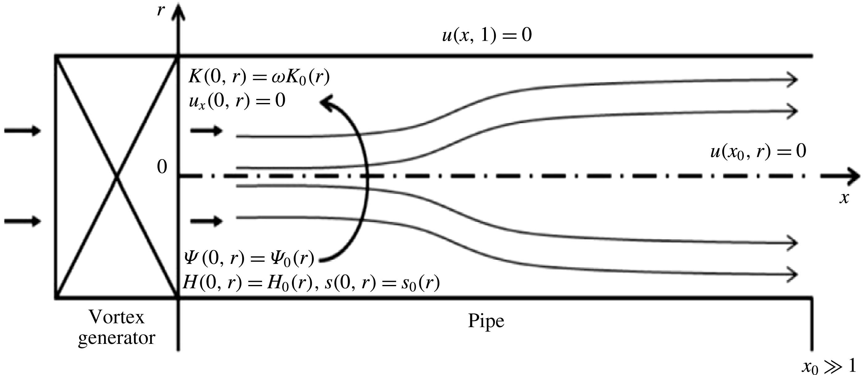
(see figure 1). Here
 $x_{0}$
is the non-dimensional pipe length. The corresponding non-dimensional velocity components are the axial velocity
 $w$
, the circumferential velocity
 $v$
and the radial velocity
 $u$
. In the entire paper, indices
 $x$
and
 $r$
represent partial derivatives with respect to
 $x$
and
 $r$
. Then, assuming axisymmetry, the continuity equation in (2.6b
) is
 $$\begin{eqnarray}\left(\unicode[STIX]{x1D70C}ru\right)_{r}+\left(\unicode[STIX]{x1D70C}rw\right)_{x}=0.\end{eqnarray}$$
From (2.13), streamfunction
 $\unicode[STIX]{x1D6F9}(x,y)$
is defined, where
 $y=r^{2}/2$
is the Stokes classical coordinate for flow problems in cylindrical coordinates,
 $0\leqslant y\leqslant 1/2$
,
 $u=-\unicode[STIX]{x1D6F9}_{x}/(\unicode[STIX]{x1D70C}\sqrt{2y})$
and
 $w=\unicode[STIX]{x1D6F9}_{y}/\unicode[STIX]{x1D70C}$
. Here, index
 $y$
represents partial derivative with respect to
 $y$
. Also, the circumferential momentum equation in (2.1) is
 $$\begin{eqnarray}\displaystyle \unicode[STIX]{x1D70C}u\left(rv\right)_{r}+\unicode[STIX]{x1D70C}w\left(rv\right)_{x}=0 & & \displaystyle\end{eqnarray}$$
Schematic diagram of a compressible swirling flow of a supercritical fluid in a pipe.

or
 $$\begin{eqnarray}\displaystyle -\unicode[STIX]{x1D6F9}_{x}\left(\sqrt{2y}v\right)_{y}+\unicode[STIX]{x1D6F9}_{y}\left(\sqrt{2y}v\right)_{x}=0. & & \displaystyle\end{eqnarray}$$
Equation (2.15) shows that the circulation function
 $K=\sqrt{2y}v$
is given by
 $K=K(\unicode[STIX]{x1D6F9})$
. This means that in a steady and axisymmetric flow the circulation function is constant along a
 $\unicode[STIX]{x1D6F9}=\text{const}.$
surface and that
 $v=K(\unicode[STIX]{x1D6F9})/\sqrt{2y}$
. In addition, equations (2.11) and (2.12) become, respectively,
 $$\begin{eqnarray}\displaystyle \left.\begin{array}{@{}c@{}}\unicode[STIX]{x1D70C}uH_{r}+\unicode[STIX]{x1D70C}wH_{x}=0,\\ \unicode[STIX]{x1D70C}us_{r}+\unicode[STIX]{x1D70C}ws_{x}=0,\end{array}\right\} & & \displaystyle\end{eqnarray}$$
or
 $$\begin{eqnarray}\displaystyle \left.\begin{array}{@{}c@{}}-\unicode[STIX]{x1D6F9}_{x}H_{y}+\unicode[STIX]{x1D6F9}_{y}H_{x}=0,\\ -\unicode[STIX]{x1D6F9}_{x}s_{y}+\unicode[STIX]{x1D6F9}_{y}s_{x}=0.\end{array}\right\} & & \displaystyle\end{eqnarray}$$
We find that
 $$\begin{eqnarray}H=H(\unicode[STIX]{x1D6F9})\quad \text{and}\quad s=s(\unicode[STIX]{x1D6F9}).\end{eqnarray}$$
This means that in a steady and axisymmetric flow the total enthalpy and specific entropy are constant along a
 $\unicode[STIX]{x1D6F9}=\text{const}.$
surface.
From (2.10) and (2.18) and the definition of the velocity components in terms of
 $\unicode[STIX]{x1D6F9}$
and its derivatives, we find that
 $$\begin{eqnarray}\displaystyle H(\unicode[STIX]{x1D6F9})=T+\frac{R}{C_{v}}\left[\frac{T}{1-\frac{1}{3}\unicode[STIX]{x1D70C}}-\frac{9}{4}\unicode[STIX]{x1D70C}+\frac{3}{16}Ma_{c}^{2}\left(\frac{\unicode[STIX]{x1D6F9}_{y}^{2}}{\unicode[STIX]{x1D70C}^{2}}+\frac{\unicode[STIX]{x1D6F9}_{x}^{2}}{2y\unicode[STIX]{x1D70C}^{2}}+\frac{K^{2}(\unicode[STIX]{x1D6F9})}{2y}\right)\right], & & \displaystyle\end{eqnarray}$$
 $$\begin{eqnarray}\displaystyle \exp \left(s(\unicode[STIX]{x1D6F9})\right)=T\left(\frac{1}{\unicode[STIX]{x1D70C}}-\frac{1}{3}\right)^{R/C_{v}}. & & \displaystyle\end{eqnarray}$$
The
 $x$
-component of the Crocco’s equation (2.9) is
 $(3/8)(R/C_{v})Ma_{c}^{2}(u\unicode[STIX]{x1D702}-v\unicode[STIX]{x1D701})=H_{x}-Ts_{x}$
, where the radial and circumferential components of the non-dimensional vorticity are
 $\unicode[STIX]{x1D701}=-v_{x}=-(1/\sqrt{2y})K_{x}$
and
 $\unicode[STIX]{x1D702}=u_{x}-w_{r}=u_{x}-\sqrt{2y}w_{y}$
, respectively. With
 $v=(K/\sqrt{2y})$
, we find that
 $$\begin{eqnarray}\displaystyle \left.\begin{array}{@{}c@{}}\displaystyle \frac{3}{8}\frac{R}{C_{v}}Ma_{c}^{2}u\left(u_{x}-\sqrt{2y}w_{y}\right)=H_{x}-\frac{3}{8}\frac{R}{C_{v}}Ma_{c}^{2}\frac{KK_{x}}{2y}-Ts_{x},\quad \text{or}\\ \displaystyle -\frac{3}{8}\frac{R}{C_{v}}Ma_{c}^{2}\frac{\unicode[STIX]{x1D6F9}_{x}}{\unicode[STIX]{x1D70C}\sqrt{2y}}\left(\!u_{x}\!-\!\sqrt{2y}w_{y}\!\right)=\left[H^{\prime }\left(\unicode[STIX]{x1D6F9}\right)-\frac{3}{8}\frac{R}{C_{v}}Ma_{c}^{2}\frac{KK^{\prime }\left(\unicode[STIX]{x1D6F9}\right)}{2y}-Ts^{\prime }\left(\unicode[STIX]{x1D6F9}\right)\right]\unicode[STIX]{x1D6F9}_{x},\quad \text{or}\\ \displaystyle \frac{3}{8}\frac{R}{C_{v}}Ma_{c}^{2}\left[\frac{1}{\unicode[STIX]{x1D70C}}\left(\frac{\unicode[STIX]{x1D6F9}_{y}}{\unicode[STIX]{x1D70C}}\right)_{y}+\frac{1}{2y\unicode[STIX]{x1D70C}}\left(\frac{\unicode[STIX]{x1D6F9}_{x}}{\unicode[STIX]{x1D70C}}\right)_{x}\right]=H^{\prime }\left(\unicode[STIX]{x1D6F9}\right)-\frac{3}{8}\frac{R}{C_{v}}Ma_{c}^{2}\frac{K(\unicode[STIX]{x1D6F9})K^{\prime }\left(\unicode[STIX]{x1D6F9}\right)}{2y}-Ts^{\prime }\left(\unicode[STIX]{x1D6F9}\right).\end{array}\right\} & & \displaystyle \nonumber\\ \displaystyle & & \displaystyle\end{eqnarray}$$
Here,
 $(\,)^{\prime }$
represents the derivative with respect to
 $\unicode[STIX]{x1D6F9}$
. The left-hand side of (2.21) represents the azimuthal vorticity in an axisymmetric compressible flow while the right-hand side includes production terms of azimuthal vorticity related to the derivatives of total enthalpy, circulation and entropy.
Equation (2.21) is a PDE for the solution of
 $\unicode[STIX]{x1D6F9}(x,y)$
. It generalizes the classical Squire–Long equation (Long Reference Long1953; Squire Reference Squire, Batchelor and Davies1956) for steady incompressible swirling flows to the case of steady compressible swirling flows of the van der Waals fluid. In (2.21), given
 $\unicode[STIX]{x1D6F9}(x,y)$
,
 $K(\unicode[STIX]{x1D6F9})$
,
 $H(\unicode[STIX]{x1D6F9})$
and
 $s(\unicode[STIX]{x1D6F9})$
, the non-dimensional density
 $\unicode[STIX]{x1D70C}(x,y)$
and temperature
 $T(x,y)$
are found from the solution of coupled system of equations (2.19) and (2.20) at all points in the flow domain.
2.2 Boundary conditions
For a flow in a rotating, finite-length, straight circular pipe of non-dimensional length
 $x_{0}$
, we consider the following boundary conditions that support (2.21) – see set-up in figure 1. At the pipe inlet at
 $x=0$
, we prescribe the profiles of the streamfunction, the circulation function, the axial derivative of radial velocity, the total head and the specific entropy by the following continuous and smooth functions, which are consistent with (2.21),
 $$\begin{eqnarray}\displaystyle \left.\begin{array}{@{}rl@{}}\unicode[STIX]{x1D6F9}(0,y) & =\unicode[STIX]{x1D6F9}_{0}(y),\quad K(0,y)=\unicode[STIX]{x1D714}K_{0}(y),\quad u_{x}(0,y)=0,\quad H(0,y)=H_{0}(y),\!\\ & \quad s(0,y)=s_{0}(y)\quad \text{for}~0\leqslant y\leqslant 1/2.\!\end{array}\right\} & & \displaystyle\end{eqnarray}$$
Here
 $\unicode[STIX]{x1D714}$
is the swirl ratio of the incoming flow, as defined in the introduction and
 $K_{0}(0)=0$
. We also assume that pressure at the inlet centreline,
 $p(0,0)=p_{CL}$
is given. Let
 $T_{CL}=T(0,0)$
and
 $\unicode[STIX]{x1D70C}_{CL}=\unicode[STIX]{x1D70C}(0,0)$
, then the non-dimensional equation of state
 $p_{CL}=(8/3)\unicode[STIX]{x1D70C}_{CL}T_{CL}/(1-(1/3)\unicode[STIX]{x1D70C}_{CL})-3\unicode[STIX]{x1D70C}_{CL}^{2}$
gives
 $p_{CL}$
in terms of the given
 $\unicode[STIX]{x1D70C}_{CL}$
and
 $T_{CL}$
. These inlet conditions may describe a compressible swirling flow that is generated by a vortex generator ahead of the pipe at a continuous and steady operation, see the experiments of Umeh et al. (Reference Umeh, Rusak, Gutmark, Villalva and Cha2010) and Umeh, Rusak & Gutmark (Reference Umeh, Rusak and Gutmark2012) who used a triple annular swirler to generate the inlet flow. The inlet condition on the axial derivative of the radial velocity allows the inlet state a degree of freedom to develop a radial velocity to account for the upstream influence of steady disturbances in the flow. In appendix A, we comment on the relationship between the inlet profiles of
 $H_{0}(y)$
and
 $s_{0}(y)$
and the inlet temperature, density, and axial and circumferential velocity profiles. The inlet radial velocity
 $u(0,y)$
is not needed for the calculation of these functions.
At the pipe outlet at
 $x=x_{0}$
, we assume that the radial velocity vanishes, i.e.
 $u(x_{0},y)=0$
, or
 $$\begin{eqnarray}\unicode[STIX]{x1D6F9}_{x}(x_{0},y)=0\quad \text{for}~0\leqslant y\leqslant 1/2.\end{eqnarray}$$
This outlet condition may represent the case of a flow in a long open pipe where the flow settles on a parallel (columnar) state ahead of the outlet. This assumption describes an apparatus with a passive discharge device. The experiments of Umeh et al. (Reference Umeh, Rusak, Gutmark, Villalva and Cha2010) show that the flow exhibits a parallel flow state at distances of six radii and higher from the inlet. The pipe non-dimensional length
 $x_{0}$
needs to be sufficiently long, say
 $x_{0}>6$
, but not too long and must be less than the entrance length for a fully developed viscous flow,
 $x_{0}\ll Re^{1/2}$
where
 $Re$
is the Reynolds number based on pipe radius
 $\bar{r}_{0}$
and characteristic velocity
 $\bar{U}_{0}$
. On the other hand, for pipes that are shorter, with
 $x_{0}<4$
, the outlet zero radial velocity may be a too strong condition on the convective flow and may fail to describe a non-columnar flow in a short pipe turning from the given inlet conditions to a passive device.
Along the pipe centreline at
 $y=0$
, we assume the axisymmetry condition,
 $\unicode[STIX]{x1D6F9}(x,0)=0$
for
 $0\leqslant x\leqslant x_{0}$
. Along the rotating pipe wall at
 $y=1/2$
, we assume constant flux,
 $\unicode[STIX]{x1D6F9}(x,1/2)=\unicode[STIX]{x1D6F9}_{w}\equiv \unicode[STIX]{x1D6F9}_{0}(1/2)$
.
By inverting
 $\unicode[STIX]{x1D6F9}(0,y)=\unicode[STIX]{x1D6F9}_{0}(y)$
to
 $y=y(\unicode[STIX]{x1D6F9})$
, we find the functions
 $K(\unicode[STIX]{x1D6F9})=\unicode[STIX]{x1D714}K_{0}(y(\unicode[STIX]{x1D6F9}))$
,
 $H(\unicode[STIX]{x1D6F9})=H_{0}(y(\unicode[STIX]{x1D6F9}))$
and
 $s(\unicode[STIX]{x1D6F9})=s_{0}(y(\unicode[STIX]{x1D6F9}))$
are defined by the inlet flow profiles in the range of
 $0\leqslant \unicode[STIX]{x1D6F9}\leqslant \unicode[STIX]{x1D6F9}_{w}$
. In addition, to accommodate possible solutions with separation zones, we assume that
 $$\begin{eqnarray}\displaystyle \left.\begin{array}{@{}c@{}}K(\unicode[STIX]{x1D6F9})=K(0)=0,\quad H(\unicode[STIX]{x1D6F9})=H(0)=H_{0},\quad s(\unicode[STIX]{x1D6F9})=s(0)=s_{0},\\ K^{\prime }(\unicode[STIX]{x1D6F9})=H^{\prime }(\unicode[STIX]{x1D6F9})=s^{\prime }(\unicode[STIX]{x1D6F9})=0\end{array}\right\} & & \displaystyle\end{eqnarray}$$
when
 $\unicode[STIX]{x1D6F9}<0$
to describe centreline breakdown zones, and
 $$\begin{eqnarray}\displaystyle \left.\begin{array}{@{}c@{}}K(\unicode[STIX]{x1D6F9})=K\left(\unicode[STIX]{x1D6F9}_{w}\right)=K_{w},\quad H(\unicode[STIX]{x1D6F9})=H\left(\unicode[STIX]{x1D6F9}_{w}\right)=H_{w},\quad s(\unicode[STIX]{x1D6F9})=s\left(\unicode[STIX]{x1D6F9}_{w}\right)=s_{w},\\ K^{\prime }(\unicode[STIX]{x1D6F9})=H^{\prime }(\unicode[STIX]{x1D6F9})=s^{\prime }(\unicode[STIX]{x1D6F9})=0\end{array}\right\} & & \displaystyle\end{eqnarray}$$
when
 $\unicode[STIX]{x1D6F9}>\unicode[STIX]{x1D6F9}_{w}$
to describe wall-separation zones.
The PDE (2.21) with the assumed boundary conditions and conditions (2.24) and (2.25) forms a well-defined problem for the solution of the flow streamfunction
 $\unicode[STIX]{x1D6F9}(x,y)$
in the domain
 $0\leqslant x\leqslant x_{0}$
and
 $0\leqslant y\leqslant 1/2$
.
A base solution of this problem for all values of
 $R/C_{v}$
,
 $Ma_{c}$
and
 $\unicode[STIX]{x1D714}$
is the columnar flow state given by
 $$\begin{eqnarray}\displaystyle \left.\begin{array}{@{}c@{}}\unicode[STIX]{x1D6F9}(x,y)=\unicode[STIX]{x1D6F9}_{0}(y),\quad K(x,y)=\unicode[STIX]{x1D714}K_{0}(y),\quad H(x,y)=H_{0}(y),\quad s(x,y)=s_{0}(y)\\ \text{for}~0\leqslant x\leqslant x_{0}\quad \text{and}\quad 0\leqslant y\leqslant 1/2.\end{array}\right\}\quad & & \displaystyle\end{eqnarray}$$
This solution is denoted as type 0 state of the swirling flow problem in a finite-length straight circular pipe. We seek to determine the possible existence of additional steady states of swirling flows in the finite-length straight circular pipe with the same
 $R/C_{v}$
,
 $Ma_{c}$
,
 $\unicode[STIX]{x1D714}$
,
 $H(\unicode[STIX]{x1D6F9})$
,
 $K(\unicode[STIX]{x1D6F9})$
,
 $s(\unicode[STIX]{x1D6F9})$
and assumed boundary conditions.
3 The columnar flow problem
A flow is defined as columnar when it is
 $x$
-independent, i.e.
 $u\equiv 0$
and
 $\unicode[STIX]{x1D6F9}=\unicode[STIX]{x1D6F9}(y)$
. Note that for a long pipe the outlet state of the solution of the PDE (2.21) is a columnar state. We consider a base, columnar state where
 $w=w_{0}(y)$
,
 $K=\unicode[STIX]{x1D714}K_{0}(y)$
,
 $T=T_{0}(y)$
,
 $p=p_{0}(y)$
,
 $\unicode[STIX]{x1D70C}=\unicode[STIX]{x1D70C}_{0}(y)$
,
 $H=H_{0}(y)$
and
 $s=s_{0}(y)$
. We construct the relationships among these profiles. From the radial momentum equation for a columnar state
 $Ma_{c}^{2}\unicode[STIX]{x1D714}^{2}\unicode[STIX]{x1D70C}_{0}(K_{0}^{2}/4y^{2})=p_{0y}$
and the relationship
 $p_{0}=p(\unicode[STIX]{x1D70C}_{0},T_{0})$
, we have
 $Ma_{c}^{2}\unicode[STIX]{x1D714}^{2}\unicode[STIX]{x1D70C}_{0}(K_{0}^{2}(y)/4y^{2})=(\unicode[STIX]{x2202}p/\unicode[STIX]{x2202}\unicode[STIX]{x1D70C})_{T_{0}}\unicode[STIX]{x1D70C}_{0y}+(\unicode[STIX]{x2202}p/\unicode[STIX]{x2202}T)_{\unicode[STIX]{x1D70C}_{0}}T_{0y}$
or
 $$\begin{eqnarray}\displaystyle Ma_{c}^{2}\unicode[STIX]{x1D714}^{2}\frac{K_{0}^{2}(y)}{4y^{2}}=\left(\frac{8}{3}\frac{T_{0}}{(1-\frac{1}{3}\unicode[STIX]{x1D70C}_{0})^{2}}-6\unicode[STIX]{x1D70C}_{0}\right)\frac{\unicode[STIX]{x1D70C}_{0y}}{\unicode[STIX]{x1D70C}_{0}}+\frac{8}{3}\frac{T_{0y}}{1-\frac{1}{3}\unicode[STIX]{x1D70C}_{0}}. & & \displaystyle\end{eqnarray}$$
Given the base state circulation
 $K_{0}(y)$
and temperature
 $T_{0}(y)$
profiles and the centreline condition
 $\unicode[STIX]{x1D70C}_{0}(0)=\unicode[STIX]{x1D70C}_{CL}$
, (3.1) is an ODE for the solution of the base state density profile
 $\unicode[STIX]{x1D70C}_{0}(y)$
. Then, the base columnar state mass flux
 $\unicode[STIX]{x1D6F9}_{0}(y)=\int _{0}^{y}\unicode[STIX]{x1D70C}_{0}({\tilde{y}})w_{0}({\tilde{y}})\,\text{d}{\tilde{y}}$
, specific total enthalpy profile
 $H_{0}(y)=T_{0}(y)+(R/C_{v})[T_{0}(y)/(1-(1/3)\unicode[STIX]{x1D70C}_{0}(y))-(9/4)\unicode[STIX]{x1D70C}_{0}(y)+(3/16)Ma_{c}^{2}(w_{0}^{2}(y)+\unicode[STIX]{x1D714}^{2}(K_{0}^{2}(y)/2y))]$
, and specific entropy profile
 $s_{0}(y)=\ln T_{0}(y)+(R/C_{v})\ln (1/\unicode[STIX]{x1D70C}_{0}(y)-1/3)$
are determined in terms of
 $w_{0}(y)$
,
 $K_{0}(y)$
,
 $T_{0}(y)$
and
 $\unicode[STIX]{x1D70C}_{0}(y)$
.
The mass flux function
 $\unicode[STIX]{x1D6F9}=\unicode[STIX]{x1D6F9}_{0}(y)$
is monotonic and can be inverted to yield
 $y=y(\unicode[STIX]{x1D6F9})$
. Then, we determine the circulation, specific total enthalpy and specific entropy functions in terms of
 $\unicode[STIX]{x1D6F9}$
,
 $$\begin{eqnarray}\displaystyle & \displaystyle K(\unicode[STIX]{x1D6F9})=\unicode[STIX]{x1D714}K_{0}\left(y\left(\unicode[STIX]{x1D6F9}\right)\right), & \displaystyle\end{eqnarray}$$
 $$\begin{eqnarray}\displaystyle & \displaystyle H(\unicode[STIX]{x1D6F9})=H_{0}(y(\unicode[STIX]{x1D713})), & \displaystyle\end{eqnarray}$$
 $$\begin{eqnarray}\displaystyle & \displaystyle s(\unicode[STIX]{x1D6F9})=s_{0}(y(\unicode[STIX]{x1D713})). & \displaystyle\end{eqnarray}$$
From (3.2)–(3.4), we find the functions derivatives in terms of
 $\unicode[STIX]{x1D6F9}$
,
 $$\begin{eqnarray}\displaystyle K^{\prime }(\unicode[STIX]{x1D6F9})=\frac{\text{d}K}{\text{d}y}\frac{\text{d}y}{\text{d}\unicode[STIX]{x1D6F9}}=\frac{\unicode[STIX]{x1D714}K_{0y}(y(\unicode[STIX]{x1D6F9}))}{\unicode[STIX]{x1D70C}_{0}(y(\unicode[STIX]{x1D6F9}))w_{0}(y(\unicode[STIX]{x1D6F9}))}, & & \displaystyle\end{eqnarray}$$
 $$\begin{eqnarray}\displaystyle H^{\prime }(\unicode[STIX]{x1D6F9}) & = & \displaystyle \frac{\text{d}H}{\text{d}y}\frac{\text{d}y}{\text{d}\unicode[STIX]{x1D6F9}}\nonumber\\ \displaystyle & = & \displaystyle \frac{1}{\unicode[STIX]{x1D70C}_{0}(y(\unicode[STIX]{x1D6F9}))w_{0}(y(\unicode[STIX]{x1D6F9}))}\left\{T_{0y}(y(\unicode[STIX]{x1D6F9}))+\frac{R}{C_{v}}\left[\frac{T_{0y}(y(\unicode[STIX]{x1D6F9}))}{1-\frac{1}{3}\unicode[STIX]{x1D70C}_{0}(y(\unicode[STIX]{x1D6F9}))}\right.\right.\nonumber\\ \displaystyle & & \displaystyle +\left.\left(\frac{T_{0}(y(\unicode[STIX]{x1D6F9}))}{3(1-\frac{1}{3}\unicode[STIX]{x1D70C}_{0}(y(\unicode[STIX]{x1D6F9})))^{2}}-\frac{9}{4}\right)\unicode[STIX]{x1D70C}_{0y}(y(\unicode[STIX]{x1D6F9}))\right]\nonumber\\ \displaystyle & & \displaystyle +\,\frac{3}{8}\frac{R}{C_{v}}Ma_{c}^{2}\left[w_{0}(y(\unicode[STIX]{x1D6F9}))w_{0y}(y(\unicode[STIX]{x1D6F9}))\vphantom{\frac{K_{0}^{2}(y(\unicode[STIX]{x1D713}))}{4y^{2}(\unicode[STIX]{x1D713})}}\right.\nonumber\\ \displaystyle & & \displaystyle \left.\left.+\,\unicode[STIX]{x1D714}^{2}\frac{K_{0}(y(\unicode[STIX]{x1D6F9}))K_{0y}(y(\unicode[STIX]{x1D6F9}))}{2y(\unicode[STIX]{x1D6F9})}-\unicode[STIX]{x1D714}^{2}\frac{K_{0}^{2}(y(\unicode[STIX]{x1D713}))}{4y^{2}(\unicode[STIX]{x1D713})}\right]\vphantom{\left[\frac{T_{0y}(y(\unicode[STIX]{x1D6F9}))}{1-\frac{1}{3}\unicode[STIX]{x1D70C}_{0}(y(\unicode[STIX]{x1D6F9}))}\right]}\right\},\end{eqnarray}$$
 $$\begin{eqnarray}\displaystyle s^{\prime }(\unicode[STIX]{x1D6F9})=\frac{\text{d}s}{\text{d}y}\frac{\text{d}y}{\text{d}\unicode[STIX]{x1D6F9}}=\frac{1}{\unicode[STIX]{x1D70C}_{0}(y(\unicode[STIX]{x1D6F9}))w_{0}(y(\unicode[STIX]{x1D6F9}))}\left\{\frac{T_{0y}(y(\unicode[STIX]{x1D6F9}))}{T_{0}(y(\unicode[STIX]{x1D6F9}))}-\frac{R}{C_{v}}\frac{\unicode[STIX]{x1D70C}_{0y}(y(\unicode[STIX]{x1D6F9}))}{(1-\frac{1}{3}\unicode[STIX]{x1D70C}_{0}(y(\unicode[STIX]{x1D6F9})))\unicode[STIX]{x1D70C}_{0}(y(\unicode[STIX]{x1D6F9}))}\right\}. & & \displaystyle \nonumber\\ \displaystyle & & \displaystyle\end{eqnarray}$$
These functions are used in (2.21).
Equation (2.21) becomes in the columnar flow case an ODE,
 $$\begin{eqnarray}\displaystyle \frac{3}{8}\frac{R}{C_{v}}Ma_{c}^{2}\frac{1}{\unicode[STIX]{x1D70C}}\left(\frac{\unicode[STIX]{x1D6F9}_{y}}{\unicode[STIX]{x1D70C}}\right)_{y}=H^{\prime }\left(\unicode[STIX]{x1D6F9}\right)-\frac{3}{8}\frac{R}{C_{v}}Ma_{c}^{2}\frac{K(\unicode[STIX]{x1D6F9})K^{\prime }\left(\unicode[STIX]{x1D6F9}\right)}{2y}-Ts^{\prime }\left(\unicode[STIX]{x1D6F9}\right), & & \displaystyle\end{eqnarray}$$
where the various functions of
 $\unicode[STIX]{x1D6F9}$
are defined in (3.2) and (3.5)–(3.7). Also,
 $T$
and
 $\unicode[STIX]{x1D70C}$
are found from the solution of the two coupled algebraic equations
 $$\begin{eqnarray}\displaystyle H(\unicode[STIX]{x1D6F9})=T+\frac{R}{C_{v}}\left[\frac{T}{1-\frac{1}{3}\unicode[STIX]{x1D70C}}-\frac{9}{4}\unicode[STIX]{x1D70C}+\frac{3}{16}Ma_{c}^{2}\left(\frac{\unicode[STIX]{x1D6F9}_{y}^{2}}{\unicode[STIX]{x1D70C}^{2}}+\frac{K^{2}(\unicode[STIX]{x1D6F9})}{2y}\right)\right], & & \displaystyle\end{eqnarray}$$
and
 $$\begin{eqnarray}\displaystyle \exp \left(s(\unicode[STIX]{x1D6F9})\right)=T\left(\frac{1}{\unicode[STIX]{x1D70C}}-\frac{1}{3}\right)^{R/C_{v}}. & & \displaystyle\end{eqnarray}$$
To simplify the solution of (3.8) we use
 $w=(\unicode[STIX]{x1D6F9}_{y}/\unicode[STIX]{x1D70C})$
and then (3.8) is equivalent to the following system of two, first-order, nonlinear ODEs in terms of
 $w(y)$
and
 $\unicode[STIX]{x1D6F9}(y)$
:
 $$\begin{eqnarray}\displaystyle & \displaystyle w_{y}=\frac{8}{3}\frac{C_{v}}{R}\frac{1}{Ma_{c}^{2}}\unicode[STIX]{x1D70C}\left[H^{\prime }\left(\unicode[STIX]{x1D6F9}\right)-\frac{3}{8}\frac{R}{C_{v}}Ma_{c}^{2}\frac{K(\unicode[STIX]{x1D6F9})K^{\prime }\left(\unicode[STIX]{x1D6F9}\right)}{2y}-Ts^{\prime }\left(\unicode[STIX]{x1D6F9}\right)\right], & \displaystyle\end{eqnarray}$$
 $$\begin{eqnarray}\displaystyle & \displaystyle \unicode[STIX]{x1D6F9}_{y}=\unicode[STIX]{x1D70C}w, & \displaystyle\end{eqnarray}$$
where
 $T$
and
 $\unicode[STIX]{x1D70C}$
are solved from (3.9) and (3.10), and the boundary conditions are
 $$\begin{eqnarray}\unicode[STIX]{x1D6F9}(0)=0,\quad \unicode[STIX]{x1D6F9}(1/2)=\unicode[STIX]{x1D6F9}_{w}=\int _{0}^{1/2}\unicode[STIX]{x1D70C}_{0}(y)w_{0}(y)\,\text{d}y.\end{eqnarray}$$
A base solution of the columnar problem (3.11) and (3.12) with conditions (3.13) is the base state,
 $w=w_{0}(y)$
,
 $K=\unicode[STIX]{x1D714}K_{0}(y)$
,
 $T=T_{0}(y)$
with
 $\unicode[STIX]{x1D70C}=\unicode[STIX]{x1D70C}_{0}(y)$
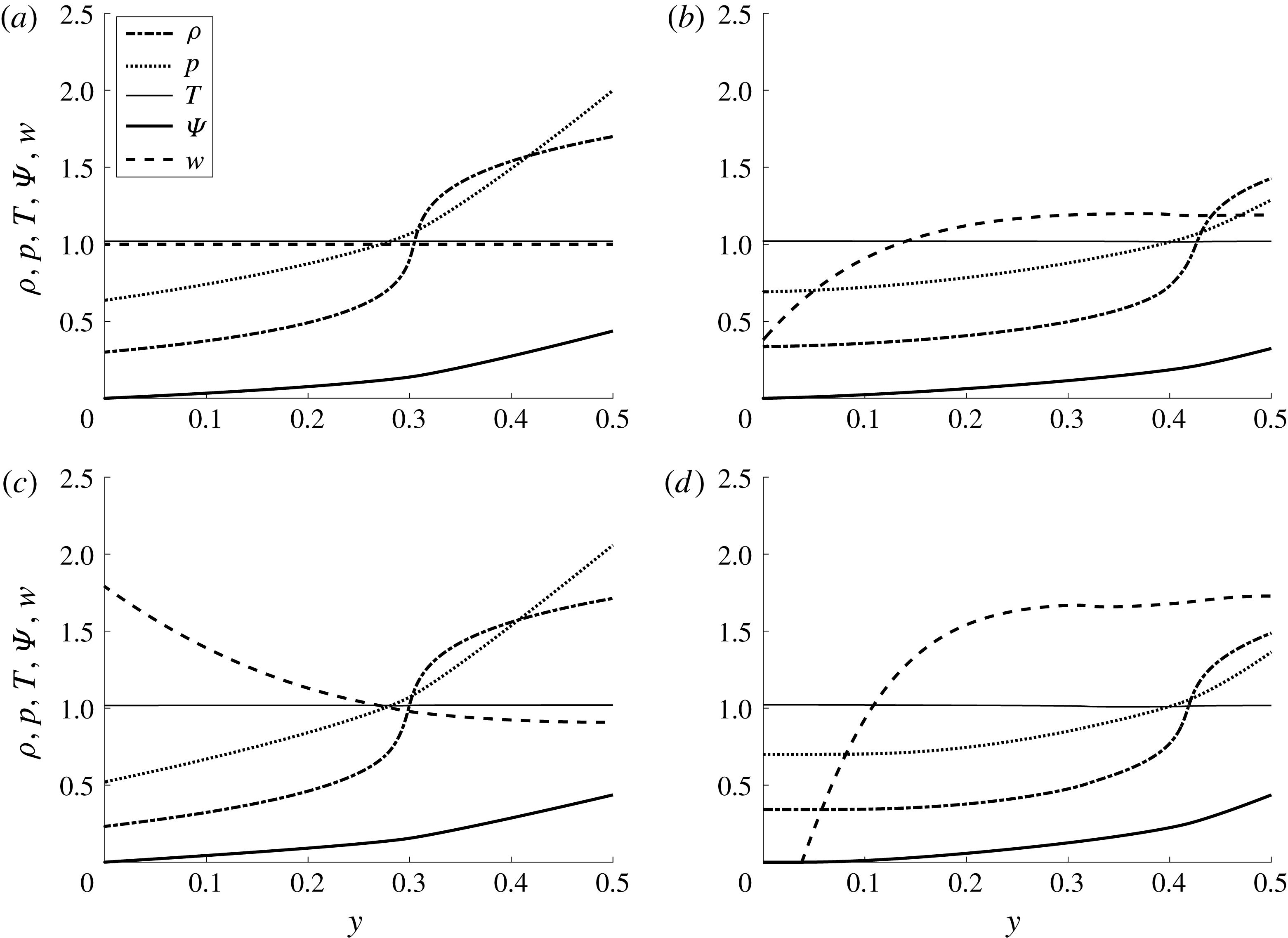
given by the solution of (3.1). This solution is denoted as type 0 solution of the columnar flow problem. Figure 2(a) presents an example of type 0 solution for the case of a solid-body rotation flow (
 $K_{0}(y)=2y$
) with a uniform axial velocity
 $(w_{0}(y)=1)$
and a constant temperature (
 $T_{0}(y)=1.02$
) at
 $Ma_{0}=0.5$
,
 $R/C_{v}=0.01$
,
 $\unicode[STIX]{x1D70C}_{CL}=0.3$
,
 $p_{CL}=0.637$
and
 $\unicode[STIX]{x1D714}=2.8$
. It can be seen in this case of a near-critical temperature, a high centreline pressure and a relatively high swirl ratio
 $\unicode[STIX]{x1D714}$
that the streamfunction
 $\unicode[STIX]{x1D6F9}$
(the solid line) increases monotonically with
 $y$
, with an increase in slope around
 $y=0.3$
. The density
 $\unicode[STIX]{x1D70C}$
(the dash-dotted line) increases from
 $0.3$
at the centreline to above the critical density at
 $y=0.304$
and to
 $1.6996$
at the wall, with a steep change in the range of
 $y$
between
 $0.25$
and
 $0.35$
where the properties vary around the critical thermodynamic point. The pressure
 $p$
(the dotted line) increases monotonically from
 $0.637$
at the centreline to above
 $1$
at
 $y=0.272$
and to
 $1.999$
at the wall, with an increase in slope around
 $y=0.3$
. The temperature
 $T$
(the thin line) and the axial velocity (the dashed line) stay constant in this type of solution. This behaviour of
 $\unicode[STIX]{x1D6F9}$
,
 $\unicode[STIX]{x1D70C}$
and
 $p$
is different from the calorically perfect-gas behaviour shown in Rusak et al. (Reference Rusak, Choi, Bourquard and Wang2015a
).
Various types of solutions of
 $\unicode[STIX]{x1D6F9}(y)$
(heavy solid line),
 $w(y)$
(dashed line),
 $T(y)$
(thin line),
 $\unicode[STIX]{x1D70C}(y)$
(dash-dotted line), and
 $p(y)$
(dotted line) for a base flow with
 $\unicode[STIX]{x1D70C}_{CL}=0.3$
,
 $T_{0}(y)=1.02$
,
 $R/C_{v}=0.01$
,
 $Ma_{0}=0.5$
. (a) Type 0 solution at
 $\unicode[STIX]{x1D714}=2.8$
; (b) type 1 solution at
 $\unicode[STIX]{x1D714}=2.45$
; (c) type 2 solution at
 $\unicode[STIX]{x1D714}=2.8$
; (d) type 3 solution at
 $\unicode[STIX]{x1D714}=2.8$
.

The study of Wang & Rusak (Reference Wang and Rusak1997) for incompressible swirling flows shows that additional solutions of the nonlinear columnar flow problem exist when the swirl ratio,
 $\unicode[STIX]{x1D714}$
, is increased above a certain value. Thereby, it shows the existence of multiple solutions of the PDE (2.21) with (2.22) and (2.23) and the appearance of vortex breakdown states in the limit of
 $Ma_{0}$
approaching zero. Similar multiple solutions and breakdown states appear in the compressible flow case of a calorically perfect gas (Rusak et al.
Reference Rusak, Choi, Bourquard and Wang2015a
) and are also expected to exist in the case of a compressible flow of a van der Waals fluid.
The system (3.11) and (3.12) is solved numerically using a fourth-order Runge–Kutta ODE integration scheme. We find that at subsonic Mach numbers there exist four additional types of solutions of the columnar problem (3.11) and (3.12). In the type 1 solution,
 $0<w(0)<w_{0}(0)$
and the solution is found by iterations until
 $w(0)$
is converged to a relative error below
 $10^{-10}$
. This type of solution describes a flow state with a decelerated flow around the centreline and an accelerated flow near the wall. In the type 2 solution,
 $w(0)>w_{0}(0)$
and again the solution is found by iterations until
 $w(0)$
is converged to a relative error below
 $10^{-10}$
. This type of solution describes a flow state with an accelerated flow around the centreline and decelerated flow near the wall. In the type 3 solution,
 $\unicode[STIX]{x1D6F9}=w=0$
for a range
 $0\leqslant y\leqslant y_{0}$
and the solution is found by iterations until
 $y_{0}$
is converged to a relative error below
 $10^{-10}$
. This type of solution describes a flow state with a stagnant (breakdown) finite zone around the centreline with radial size of
 $\sqrt{2y_{0}}$
. In the type 4 solution,
 $\unicode[STIX]{x1D6F9}=\unicode[STIX]{x1D6F9}_{w}$
and
 $w=0$
for a range
 $y_{w}\leqslant y\leqslant 1/2$
and the solution is found by iterations until
 $y_{w}$
is converged to a relative error below
 $10^{-10}$
. This type of solution describes a flow state with a quasi-stagnation finite zone attached to the wall, where the radial and axial velocity components vanish but the circumferential velocity is
 $K(\unicode[STIX]{x1D6F9}_{w})/\sqrt{2y}$
. The radial location of the interface of this zone is at
 $\sqrt{2y_{w}}$
. For the cases studied in this paper, the type 4 solutions may appear at swirl level beyond the range investigated.
Representative examples of type 1, type 2 and type 3 solutions for a base solid-body rotation flow with a uniform axial velocity
 $w_{0}(y)=1$
and a constant temperature
 $T_{0}(y)=1.02$
at
 $Ma_{0}=0.5$
,
 $R/C_{v}=0.01$
,
 $\unicode[STIX]{x1D70C}_{CL}=0.3$
and
 $p_{CL}=0.637$
are shown in figures 2(b) (at
 $\unicode[STIX]{x1D714}=2.45$
), 2(c) (at
 $\unicode[STIX]{x1D714}=2.8$
) and 2(d) (at
 $\unicode[STIX]{x1D714}=2.8$
), respectively. Each of the panels describes the computed streamfunction
 $\unicode[STIX]{x1D6F9}(y)$
, the axial velocity
 $w(y)$
, the temperature
 $T(y)$
, the density
 $\unicode[STIX]{x1D70C}(y)$
and the pressure
 $p(y)$
. With respect to the base flow state, the type 1 solution describes a state where around the centreline there is a decelerated flow (
 $w(0)=0.379<1$
) and higher temperature (
 $T(0)=1.021$
), density (
 $\unicode[STIX]{x1D70C}(0)=0.335$
) and pressure (
 $p(0)=0.691$
). Near the wall there is an accelerated flow (
 $w(1/2)=1.190>1$
) with lower temperature (
 $T(1/2)=1.019$
), density (
 $\unicode[STIX]{x1D70C}(1/2)=1.428$
) and pressure (
 $p(1/2)=1.228$
) (see figure 2
b). The type 2 solution describes a state where near the centreline there is an accelerated flow (
 $w(0)=1.789>1$
) with lower temperature (
 $T(0)=1.017$
), density (
 $\unicode[STIX]{x1D70C}(0)=0.232$
) and pressure (
 $p(0)=0.521$
) with respect to the base flow. Near the wall there is a decelerated flow (
 $w(1/2)=0.908<1$
) and higher temperature (
 $T(1/2)=1.0202$
), density (
 $\unicode[STIX]{x1D70C}(1/2)=1.171$
) and pressure (
 $p(1/2)=2.059$
) (see figure 2
c). The type 3 solution describes a state with a finite-size stagnation zone of size
 $y_{0}=0.038$
, where
 $\unicode[STIX]{x1D6F9}(y)=w(y)=v(y)=0$
in the range
 $0\leqslant y\leqslant y_{0}$
, with higher temperature (
 $T(0)=1.021$
), density (
 $\unicode[STIX]{x1D70C}(0)=0.342$
) and pressure (
 $p(0)=0.7004$
) inside the stagnation zone, and with an accelerated axial velocity (
 $w(1/2)=1.728$
) and lower temperature (
 $T(1/2)=1.017$
), density (
 $\unicode[STIX]{x1D70C}(1/2)=1.488$
) and pressure (
 $p(1/2)=1.364$
) near the wall (see figure 2
d). The centreline velocity
 $w(0)$
of each type of solution as a function of the inlet swirl ratio
 $\unicode[STIX]{x1D714}$
, Mach number
 $Ma_{0}$
,
 $R/C_{v}$
and
 $\unicode[STIX]{x1D70C}_{CL}$
is used in § 4 as a representative parameter of the solutions.
We conjecture that type 0 to 3 solutions are the only types of solutions of the ODE problem that have physical relevance in the range of operational parameters studied. The proof that there are no other solutions is beyond the scope of the interests of the present paper. These solutions determine for a long pipe the outlet profile and the corresponding nature of the flow state in a finite-length pipe, i.e. the type 0 solutions form the columnar type 0 states of the PDE (2.21), the type 1 solutions form centreline-decelerated flow states, the type 2 solutions form centreline-accelerated flow states, and the type 3 solutions form vortex-breakdown states with a finite-size stagnation zone that starts from a point on the centreline.
4 Computed examples
In this section we focus on the case of an inlet solid-body rotation flow for which the base circulation function is
 $K_{0}(y)=2y$
, the axial velocity is uniform,
 $w_{0}(y)=1$
, and the temperature is constant,
 $T_{0}(y)=1.02$
. In all examples we assume that the inlet centreline Mach number is
 $Ma_{0}=0.5$
and the fluid is characterized by
 $R/C_{v}=0.01$
. The choice of
 $Ma_{0}=0.5$
provides a representative case with subsonic flow and sufficient compressibility effects but without any transonic effects and shock waves. This flow Mach number was also used in Rusak et al. (Reference Rusak, Choi, Bourquard and Wang2015a
). The choice of
 $R/C_{v}=0.01$
represents aviation hydrocarbon fuels with heavy molecules such as those used in the studies of Crook et al. (Reference Crook, Rachedi and Sojka2007) and Rachedi et al. (Reference Rachedi, Crook and Sojka2010).
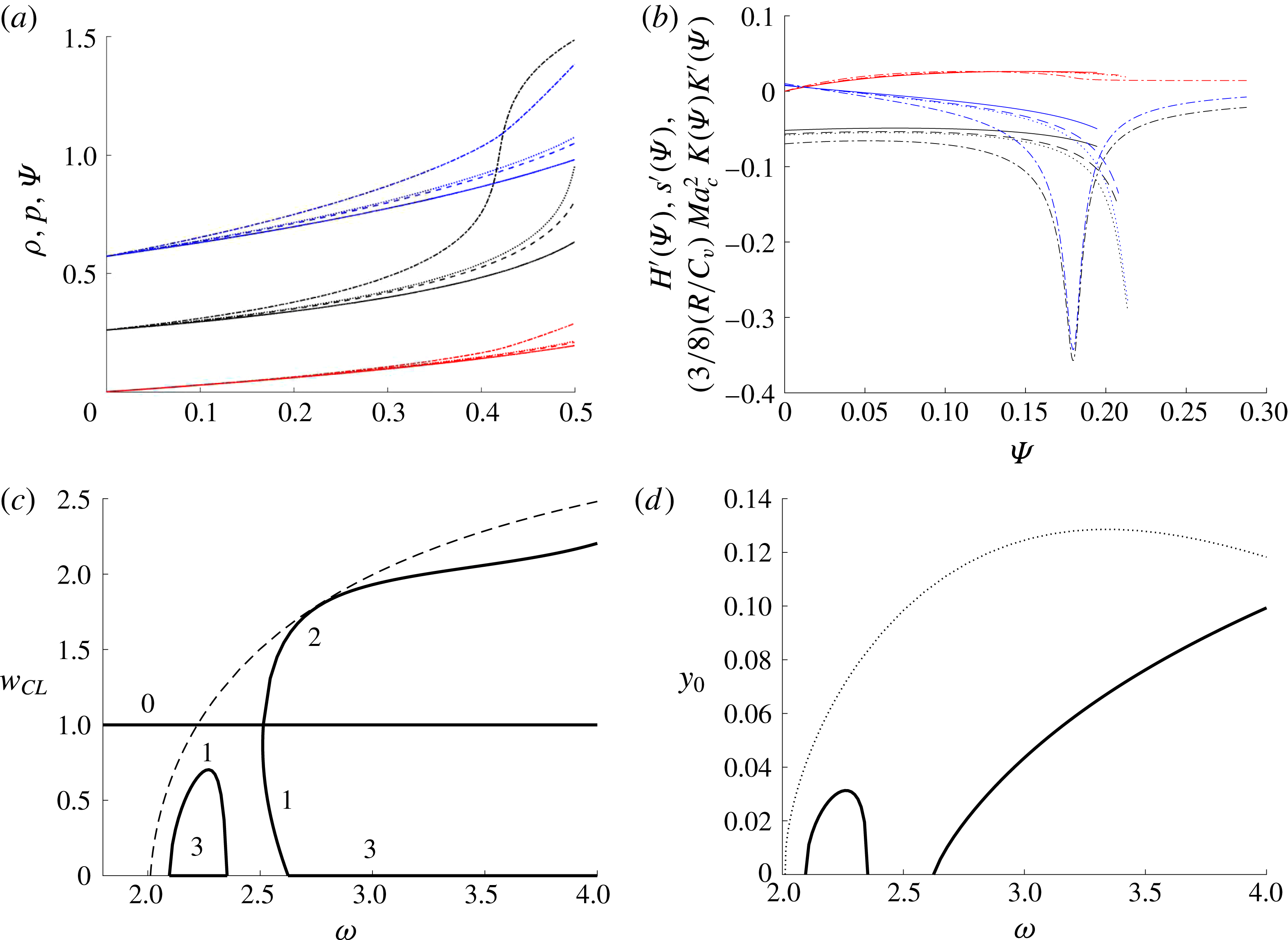
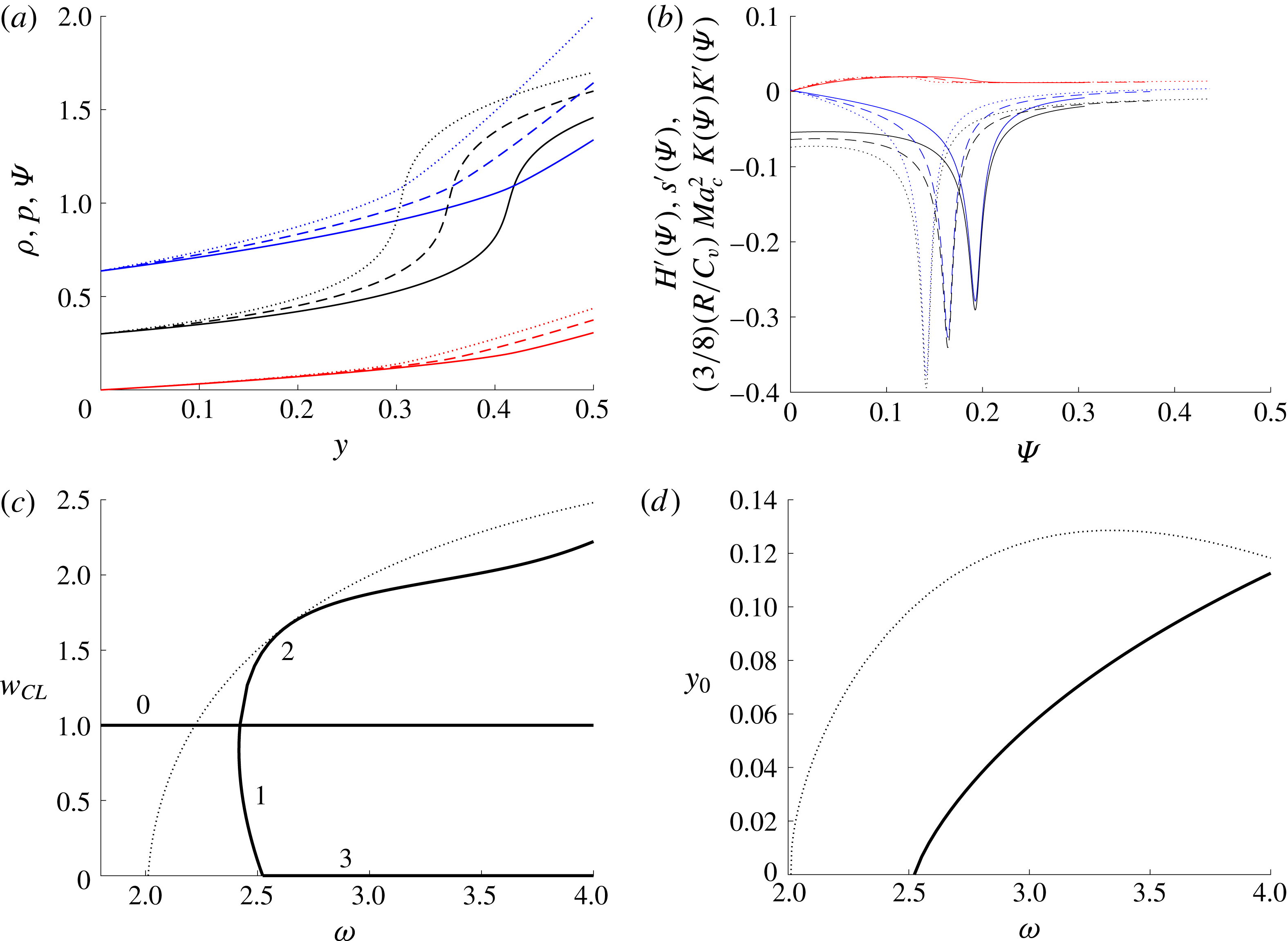
We investigate the fluid flow behaviour according to (3.11)–(3.13) with the sequential increase of the base flow centreline density
 $\unicode[STIX]{x1D70C}_{CL}$
from a near-zero value (representing a calorically perfect-gas behaviour) to
 $1$
(representing the behaviour of a real thermodynamically supercritical fluid). We chose nine cases of
 $\unicode[STIX]{x1D70C}_{CL}$
to study the swirling flow nature. These cases were chosen carefully to represent changes of flow behaviour, with special attention to values of
 $\unicode[STIX]{x1D70C}_{CL}$
where the critical swirls exhibit significant changes with
 $\unicode[STIX]{x1D70C}_{CL}$
. For each value of the base flow
 $\unicode[STIX]{x1D70C}_{CL}$
, we first describe the resulting base flow profiles of density, pressure and streamfunction as a function of
 $y$
(panels (a) in these figures) and the related functions
 $(3/8)(R/C_{v})Ma_{c}^{2}K(\unicode[STIX]{x1D6F9})K^{\prime }(\unicode[STIX]{x1D6F9})$
,
 $H^{\prime }(\unicode[STIX]{x1D6F9})$
and
 $s^{\prime }(\unicode[STIX]{x1D6F9})$
at various levels of
 $\unicode[STIX]{x1D714}$
(panels (b)). We then derive by successive continuation method the bifurcation diagrams of solutions of swirling flows in terms of the computed centreline axial velocity
 $w_{CL}=w(0)$
for each solution as a function of the incoming flow swirl ratio
 $\unicode[STIX]{x1D714}$
(panels (c)). We also provide the size
 $y_{0}$
of the breakdown zones of type 3 solutions as a function of
 $\unicode[STIX]{x1D714}$
(panels (d)). Note that each of the nine cases presented below shows a distinctive behaviour, specifically in terms of the bifurcation diagrams, that is not found in the other cases.
4.1 Case 1: the calorically perfect-gas limit (
 $\unicode[STIX]{x1D70C}_{CL}=10^{-6}$
)

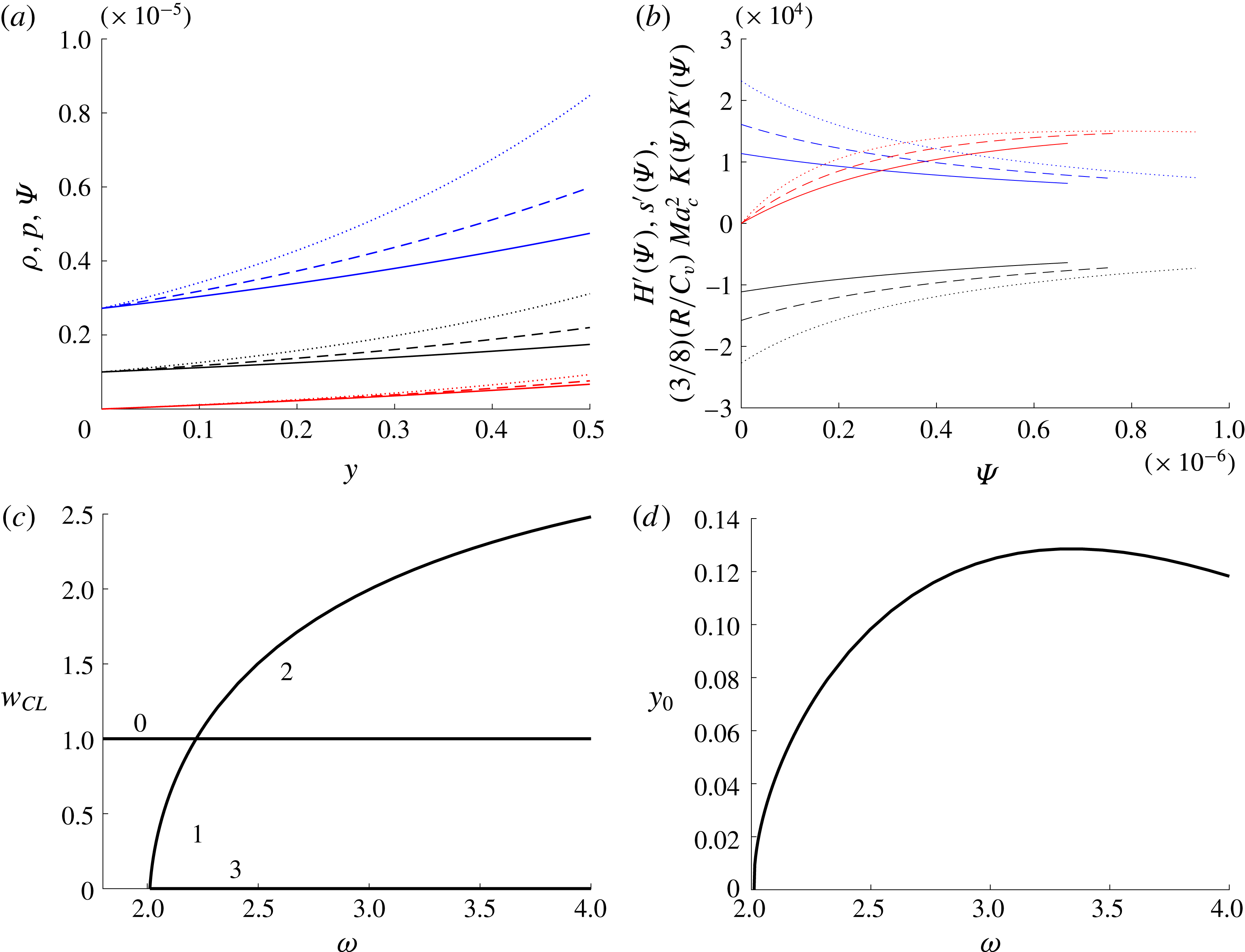
In this case (figure 3), the base flow density
 $\unicode[STIX]{x1D70C}$
, pressure
 $p$
and streamfunction
 $\unicode[STIX]{x1D6F9}$
increase monotonically with
 $y$
for all
 $\unicode[STIX]{x1D714}$
and increase with
 $\unicode[STIX]{x1D714}$
at all
 $y$
(figure 3(a); note that the scale of these functions is on the order of
 $10^{-6}$
) and flow is a calorically perfect gas for all
 $y$
and
 $\unicode[STIX]{x1D714}$
studied. The function
 $(3/8)(R/C_{v})Ma_{c}^{2}K(\unicode[STIX]{x1D6F9})K^{\prime }(\unicode[STIX]{x1D6F9})$
is positive and increases monotonically with
 $\unicode[STIX]{x1D6F9}$
, while
 $H^{\prime }(\unicode[STIX]{x1D6F9})$
is positive but decreases monotonically with
 $\unicode[STIX]{x1D6F9}$
, and
 $s^{\prime }(\unicode[STIX]{x1D6F9})$
is negative and increases monotonically with
 $\unicode[STIX]{x1D6F9}$
(figure 3(b); note that the range of
 $\unicode[STIX]{x1D6F9}$
increases with
 $\unicode[STIX]{x1D714}$
since
 $\unicode[STIX]{x1D6F9}_{w}=\unicode[STIX]{x1D6F9}(1/2)$
increases as a function of
 $\unicode[STIX]{x1D714}$
, see figure 3(a)). The resulting bifurcation diagram (figure 3
c) shows that type 0 solution with
 $w_{CL}=1$
exists for all
 $\unicode[STIX]{x1D714}$
. At
 $\unicode[STIX]{x1D714}=\unicode[STIX]{x1D714}_{c}=2.218$
, type 1 and type 2 solutions bifurcate from the type 0 branch of solutions. The type 1 branch of solutions with
 $0<w_{CL}<1$
develops with the decrease of
 $\unicode[STIX]{x1D714}$
from
 $\unicode[STIX]{x1D714}_{c}=2.218$
to
 $\unicode[STIX]{x1D714}_{\ast }=2.012$
. The type 2 solutions with
 $w_{CL}>1$
develop as
 $\unicode[STIX]{x1D714}$
increases above
 $\unicode[STIX]{x1D714}_{c}=2.218$
. Type 3 breakdown solutions with
 $w_{CL}=0$
develop with the increase of
 $\unicode[STIX]{x1D714}$
above
 $\unicode[STIX]{x1D714}_{\ast }=2.012$
. The related size
 $y_{0}$
of the type 3 solutions increases with the increase of
 $\unicode[STIX]{x1D714}$
from
 $\unicode[STIX]{x1D714}_{\ast }=2.012$
to
 $\unicode[STIX]{x1D714}=3.3$
and then decreases with further increase of
 $\unicode[STIX]{x1D714}$
(figure 3
d).
Case 1: Perfect-gas limit,
 $\unicode[STIX]{x1D70C}_{CL}=10^{-6}$
,
 $T_{0}=1.02$
,
 $Ma_{0}=0.5$
,
 $R/C_{v}=0.01$
. In panels (a,b)
 $\unicode[STIX]{x1D714}=2.1$
(solid lines),
 $\unicode[STIX]{x1D714}=2.5$
(dashed lines) and
 $\unicode[STIX]{x1D714}=3$
(dotted lines): (a) solutions of the base columnar flow density
 $\unicode[STIX]{x1D70C}$
(black lines), pressure
 $p$
(blue lines) and streamfunction
 $\unicode[STIX]{x1D6F9}$
(red lines) as a function of
 $y$
; (b) the functions
 $H^{\prime }(\unicode[STIX]{x1D6F9})$
(blue lines),
 $s^{\prime }(\unicode[STIX]{x1D6F9})$
(black lines) and
 $(3/8)(R/C_{v})Ma_{c}^{2}K(\unicode[STIX]{x1D6F9})K^{\prime }(\unicode[STIX]{x1D6F9})$
(red lines) as a function of
 $\unicode[STIX]{x1D6F9}$
; (c) the bifurcation diagram of solutions of
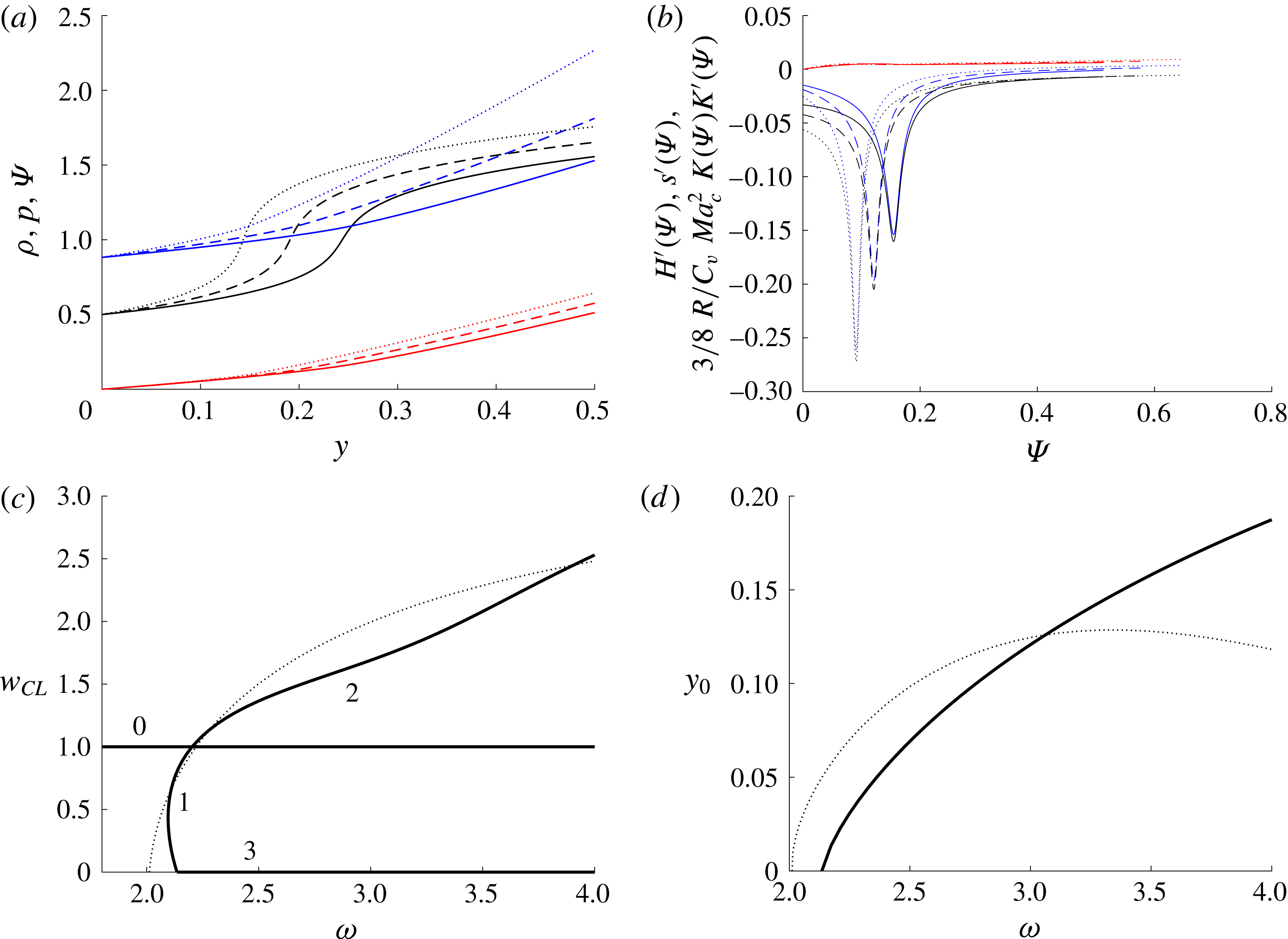
 $w_{CL}$
against
 $\unicode[STIX]{x1D714}$
; (d) the size of the breakdown zone
 $y_{0}$
as a function of
 $\unicode[STIX]{x1D714}$
for type 3 solutions.

The swirling flow behaviour in the perfect-gas limit case is similar to that reported in Rusak et al. (Reference Rusak, Choi, Bourquard and Wang2015a
) where the dynamics of swirling flows of a calorically perfect gas in a straight pipe was studied. Moreover, the present results match with the previous results when
 $R/C_{v}=0.4$
(or the ratio of specific heat is
 $\unicode[STIX]{x1D6FE}=1.4$
) and
 $Ma_{0}=0.5$
are used.
The results of the calorically perfect-gas case in Rusak et al. (Reference Rusak, Choi and Lee2007, Reference Rusak, Choi, Bourquard and Wang2015a
) show for a long pipe that the columnar flow (type 0) states are asymptotically stable when
 $0<\unicode[STIX]{x1D714}<\unicode[STIX]{x1D714}_{c}$
and unstable when
 $\unicode[STIX]{x1D714}>\unicode[STIX]{x1D714}_{c}$
. Similarly, the centreline-decelerated flow (type 1) states are also unstable in the range
 $\unicode[STIX]{x1D714}_{\ast }<\unicode[STIX]{x1D714}<\unicode[STIX]{x1D714}_{c}$
, while the centreline-accelerated flow (type 2) states are asymptotically stable when
 $\unicode[STIX]{x1D714}>\unicode[STIX]{x1D714}_{c}$
. The breakdown (type 3) states are found to be attractors of flow dynamics when
 $\unicode[STIX]{x1D714}>\unicode[STIX]{x1D714}_{\ast }$
. Therefore, the columnar states attract the long-term flow evolution of a perturbed columnar state when
 $0<\unicode[STIX]{x1D714}<\unicode[STIX]{x1D714}_{c}$
while the breakdown states dominate the long-term evolution of a perturbed columnar flow as
 $\unicode[STIX]{x1D714}$
is increased above
 $\unicode[STIX]{x1D714}_{\ast }$
. In the overlap range
 $\unicode[STIX]{x1D714}_{\ast }<\unicode[STIX]{x1D714}<\unicode[STIX]{x1D714}_{c}$
, the evolution is determined by the initial perturbations and the domains of attraction of the columnar and breakdown states, separated by the branch of type 1 states.
4.2 Case 2:
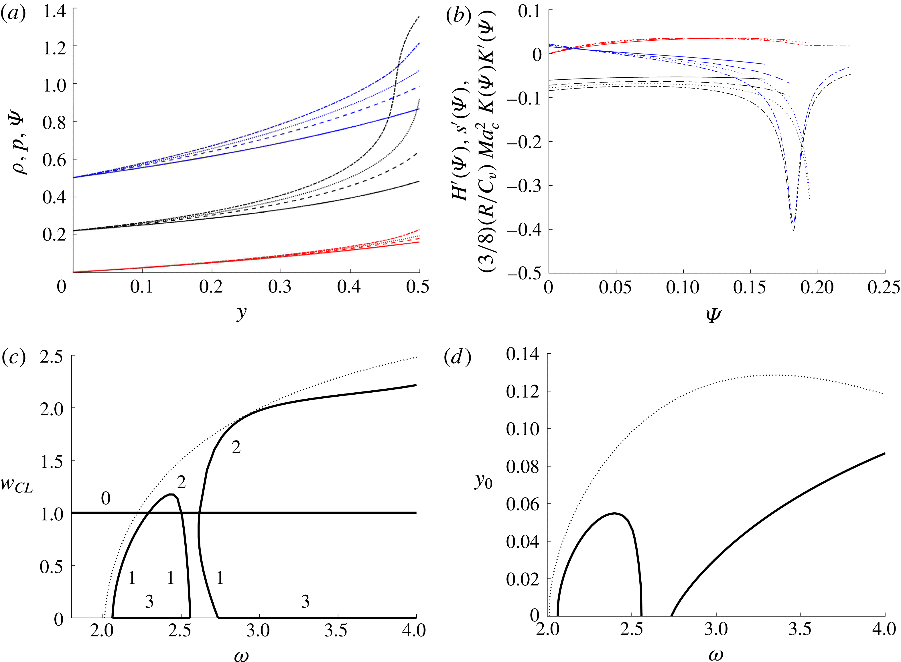
$\unicode[STIX]{x1D70C}_{CL}=0.1$

With the increase of the base flow centreline density
 $\unicode[STIX]{x1D70C}_{CL}$
from near-zero values to 0.1, the flow behaviour changes from that of the calorically perfect gas found in Rusak et al. (Reference Rusak, Choi, Bourquard and Wang2015a
) since the base flow density and pressure achieve at
 $\unicode[STIX]{x1D714}>3.3$
values around and above 1 (the critical thermodynamic point) near the pipe wall at
 $y=1/2$
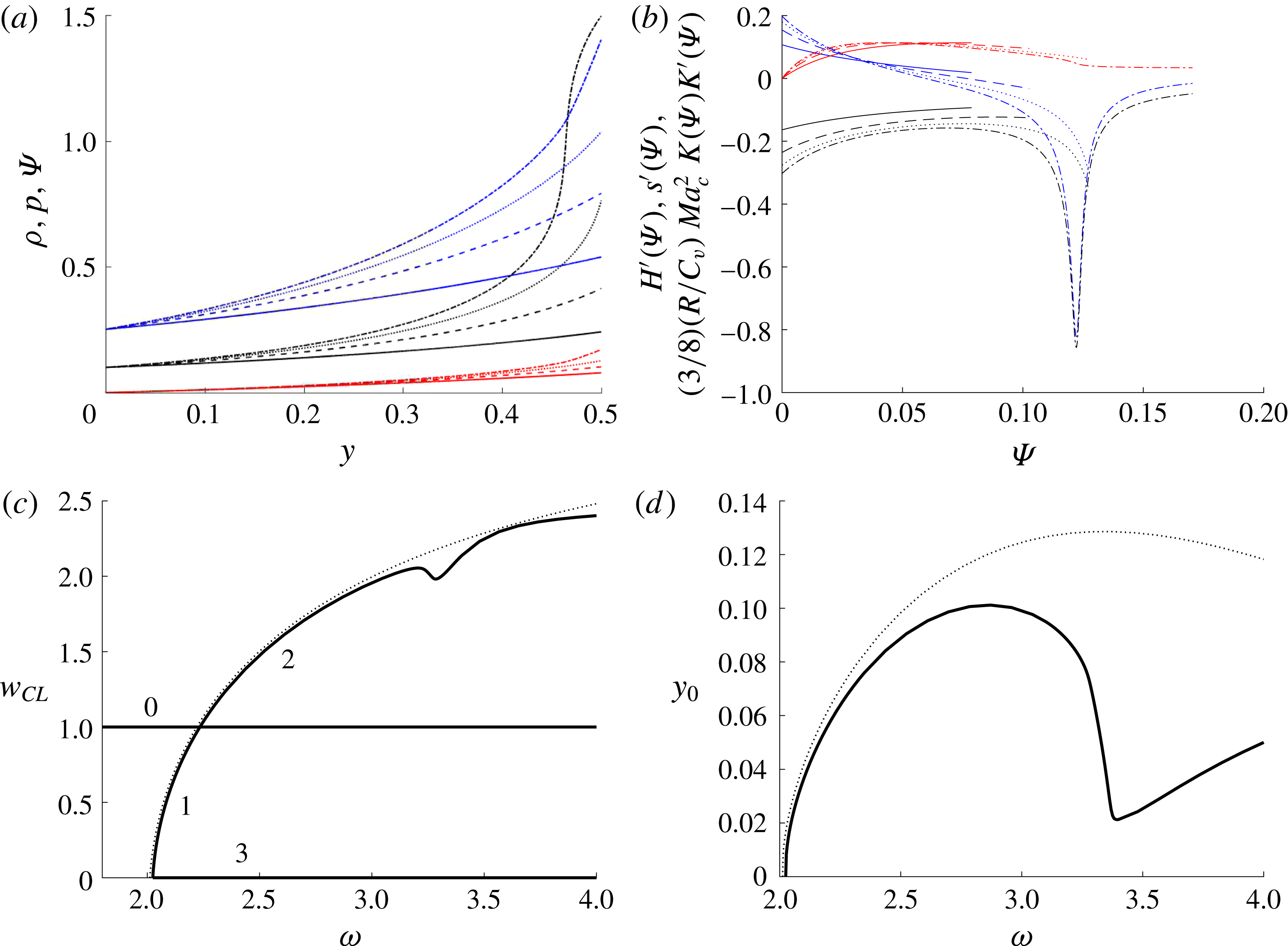
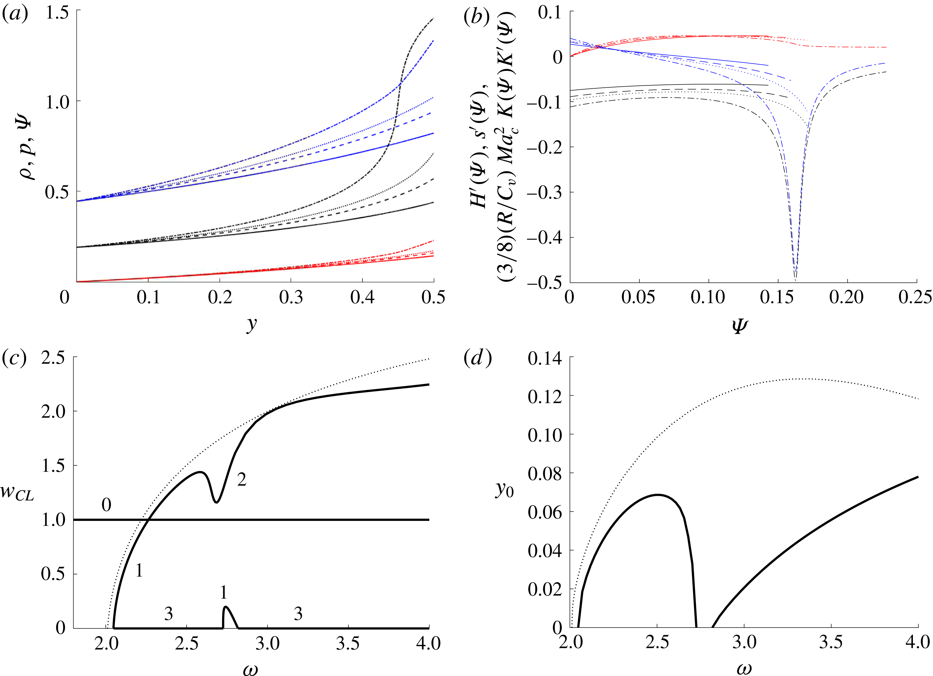
(figure 4
a). The streamfunction
 $\unicode[STIX]{x1D6F9}_{0}(y)$
remains monotonic with
 $y$
but increases its slope near the wall. It is important to also note that the density
 $\unicode[STIX]{x1D70C}_{0}(y)$
has a positive curvature for all
 $y$
when
 $\unicode[STIX]{x1D714}\leqslant 3.3$
. However, the high swirl causes
 $\unicode[STIX]{x1D70C}_{0}(y)$
to increase rapidly within the domain as it varies around 1 and to change its curvature when it is above 1, as
 $\unicode[STIX]{x1D714}$
increases above
 $3.3$
. This behaviour of
 $\unicode[STIX]{x1D70C}_{0}(y)$
can be seen directly from (3.1). The term
 $(8/3)(T_{0}/(1-(1/3)\unicode[STIX]{x1D70C}_{0})^{2})-6\unicode[STIX]{x1D70C}_{0}$
is positive for all
 $0<\unicode[STIX]{x1D70C}_{0}<3$
but decreases as
 $\unicode[STIX]{x1D70C}_{0}$
increases, reaches a minimum at
 $\unicode[STIX]{x1D70C}_{0}=1$
with near-zero value and then increases with increase of
 $\unicode[STIX]{x1D70C}_{0}$
above 1. As a result, at near-critical thermodynamic conditions, the derivative
 $\unicode[STIX]{x1D70C}_{0y}$
is positive, increases with
 $y$
as
 $\unicode[STIX]{x1D70C}_{0}$
tends towards 1, reaches a large maximum value when
 $\unicode[STIX]{x1D70C}_{0}=1$
, and then decreases with increase of
 $\unicode[STIX]{x1D70C}_{0}$
above 1. This behaviour of
 $\unicode[STIX]{x1D70C}_{0}$
strongly affects the functions
 $H^{\prime }(\unicode[STIX]{x1D6F9})$
and
 $s^{\prime }(\unicode[STIX]{x1D6F9})$
.
Case 2:
 $\unicode[STIX]{x1D70C}_{CL}=0.1$
,
 $T_{0}=1.02$
,
 $Ma_{0}=0.5$
,
 $R/C_{v}=0.01$
. In panels (a,b)
 $\unicode[STIX]{x1D714}=2.5$
(solid lines),
 $\unicode[STIX]{x1D714}=3$
(dashed lines),
 $\unicode[STIX]{x1D714}=3.25$
(dotted lines) and
 $\unicode[STIX]{x1D714}=3.4$
(dash-dotted lines). In panels (c,d) the calorically perfect-gas bifurcation diagram is shown for reference (dotted line). (a) Solutions of the base columnar flow density
 $\unicode[STIX]{x1D70C}$
(black lines), pressure
 $p$
(blue lines) and streamfunction
 $\unicode[STIX]{x1D6F9}$
(red lines) as a function of
 $y$
; (b) the functions
 $H^{\prime }(\unicode[STIX]{x1D6F9})$
(blue lines),
 $s^{\prime }(\unicode[STIX]{x1D6F9})$
(black lines) and
 $(3/8)(R/C_{v})Ma_{c}^{2}K(\unicode[STIX]{x1D6F9})K^{\prime }(\unicode[STIX]{x1D6F9})$
(red lines) as a function of
 $\unicode[STIX]{x1D6F9}$
; (c) the bifurcation diagram of solutions of
 $w_{CL}$
against
 $\unicode[STIX]{x1D714}$
; (d) the size of the breakdown zone
 $y_{0}$
as a function of
 $\unicode[STIX]{x1D714}$
for type 3 solutions.

The related function
 $(3/8)(R/C_{v})Ma_{c}^{2}K(\unicode[STIX]{x1D6F9})K^{\prime }(\unicode[STIX]{x1D6F9})$
is positive for the range of
 $\unicode[STIX]{x1D714}$
studied but reaches a maximum value around
 $\unicode[STIX]{x1D6F9}=0.06$
and then decreases with increase of
 $\unicode[STIX]{x1D6F9}$
towards
 $\unicode[STIX]{x1D6F9}_{w}$
(figure 4
b). The function
 $H^{\prime }(\unicode[STIX]{x1D6F9})$
decreases monotonically with
 $\unicode[STIX]{x1D6F9}$
for
 $\unicode[STIX]{x1D714}\leqslant 3.3$
and becomes negative in a certain range of
 $\unicode[STIX]{x1D6F9}$
. However, when
 $\unicode[STIX]{x1D714}=3.4$
, near- and above-critical thermodynamic properties exist near the wall (figure 4
a). Then, the function
 $H^{\prime }(\unicode[STIX]{x1D6F9})$
decreases significantly to negative values, reaches a minimum at
 $\unicode[STIX]{x1D6F9}=0.122$
, and increases as
 $\unicode[STIX]{x1D6F9}$
increases towards
 $\unicode[STIX]{x1D6F9}_{w}$
, yet exhibiting negative values near the wall. The function
 $s^{\prime }(\unicode[STIX]{x1D6F9})$
is negative for all
 $\unicode[STIX]{x1D714}$
studied and increases monotonically with
 $\unicode[STIX]{x1D6F9}$
when
 $\unicode[STIX]{x1D714}<3$
. For
 $3<\unicode[STIX]{x1D714}\leqslant 3.3$
, this function reaches a maximum value and then decreases with
 $\unicode[STIX]{x1D6F9}$
. However, when
 $\unicode[STIX]{x1D714}=3.4$
and near- and above-critical thermodynamic properties exist near the wall (figure 4
a), the function
 $s^{\prime }(\unicode[STIX]{x1D6F9})$
decreases significantly to negative values, reaches a minimum at
 $\unicode[STIX]{x1D6F9}=0.122$
, and then increases as
 $\unicode[STIX]{x1D6F9}$
increases towards
 $\unicode[STIX]{x1D6F9}_{w}$
, yet exhibiting negative values near the wall (figure 4
b). At the specific inlet conditions (
 $T_{0}(y)=1.02=\text{const}.$
,
 $w_{0}(y)=1=\text{const}.$
) and at near-critical thermodynamic conditions (
 $\unicode[STIX]{x1D70C}_{0}\sim 1$
), equations (3.6) and (3.7) show that the behaviour of the functions
 $H^{\prime }(\unicode[STIX]{x1D6F9})$
and
 $s^{\prime }(\unicode[STIX]{x1D6F9})$
is directly related to
 $-\unicode[STIX]{x1D70C}_{0y}$
. Therefore, when
 $\unicode[STIX]{x1D714}$
is increased and above-critical thermodynamic conditions appear near the wall, the functions
 $H^{\prime }(\unicode[STIX]{x1D6F9})$
and
 $s^{\prime }(\unicode[STIX]{x1D6F9})$
decrease as
 $\unicode[STIX]{x1D70C}_{0}$
tends towards 1, reach a large negative minimum when
 $\unicode[STIX]{x1D70C}_{0}=1$
, and then increase with increase of
 $\unicode[STIX]{x1D70C}_{0}$
above 1.
This significant change of the behaviour of the functions
 $(3/8)(R/C_{v})Ma_{c}^{2}K(\unicode[STIX]{x1D6F9})$
 $K^{\prime }(\unicode[STIX]{x1D6F9})$
,
 $H^{\prime }(\unicode[STIX]{x1D6F9})$
and
 $s^{\prime }(\unicode[STIX]{x1D6F9})$
at
 $\unicode[STIX]{x1D714}>3.3$
affects the computed solutions of (3.11)–(3.13). The results are shown in the bifurcation diagram in figure 4(c). Again, the base type 0 branch of solutions exists for all
 $\unicode[STIX]{x1D714}$
. The type 1 and 2 solutions bifurcate at a slightly higher swirl level than that in the calorically perfect-gas case,
 $\unicode[STIX]{x1D714}_{c}=2.235$
. The type 3 breakdown solutions also start at a higher swirl ratio
 $\unicode[STIX]{x1D714}_{\ast }=2.02$
. However, there is a clear change in the behaviour of type 2 and type 3 solutions when
 $3.2<\unicode[STIX]{x1D714}<3.5$
, when near- and above-critical thermodynamic pressure and density are achieved near the wall. The type 2 states exhibit a slight decrease in
 $w_{CL}$
with a minimum at
 $\unicode[STIX]{x1D714}=3.4$
. Above
 $\unicode[STIX]{x1D714}=3.5$
, the minima of
 $H^{\prime }(\unicode[STIX]{x1D6F9})$
and
 $s^{\prime }(\unicode[STIX]{x1D6F9})$
move away from the wall into the bulk and become more negative. Then, the branch of type 2 states continues monotonically with the increase of
 $\unicode[STIX]{x1D714}$
above
 $3.5$
. The type 3 solutions exhibit a size of
 $y_{0}$
that increases with
 $\unicode[STIX]{x1D714}$
in the range
 $2.02<\unicode[STIX]{x1D714}<2.87$
, decreases in the range
 $2.87<\unicode[STIX]{x1D714}<3.4$
and then increases again when
 $\unicode[STIX]{x1D714}>3.4$
, see figure 4(d).
In order to shed additional physical insight into the nature of the various types of solutions, we describe in the phase diagram in figure 5 the variations of the pressure (
 $p$
) as a function of the specific volume (
 $1/\unicode[STIX]{x1D70C}$
) for the type 0, type 2 and type 3 solutions computed at a representative high swirl ratio,
 $\unicode[STIX]{x1D714}=3.4$
. Also shown in this figure is the saturation line as computed from Maxwell construction condition (Maxwell Reference Maxwell1875). Owing to the relatively low
 $R/C_{v}=0.01$
, the change of temperature from the constant
 $T_{0}=1.02$
is not significant for all three types of solutions. However, the changes of pressure and specific volume induced by the axial and circumferential velocities are visible, specifically at the high level of swirl ratio. The base type 0 solution (black solid line) ranges along the isothermal curve
 $T_{0}=1.02$
from
 $1/\unicode[STIX]{x1D70C}=10$
and
 $p=0.2514$
at the centreline, that is well inside the vapour region, to
 $1/\unicode[STIX]{x1D70C}=0.6681$
and
 $p=1.404$
at the wall, that is, in the thermodynamically supercritical dense-flow region. The type 2 solution (red solid line), with accelerated axial velocity near the centreline and decelerated velocity near the wall, exhibits as a result a decrease of pressure and an increase of specific volume near the centreline and an increase of pressure and slight decrease of specific volume near the wall. The type 3 solution (blue solid line), with decelerated axial velocity near the centreline and accelerated velocity near the wall, exhibits as a result an increase of pressure and a decrease of specific volume near the centreline and a decrease of pressure and slight increase of specific volume near the wall. We note that solutions for high swirl levels with
 $\unicode[STIX]{x1D714}>3.4$
exhibit a similar behaviour.
Variations of pressure (
 $p$
) as a function of fluid specific volume (
 $1/\unicode[STIX]{x1D70C}$
) for type 0 (black solid line), type 2 (red solid line) and type 3 (blue solid line) solutions at inlet conditions of case 2:
 $\unicode[STIX]{x1D70C}_{CL}=0.1$
,
 $T_{0}=1.02$
,
 $Ma_{0}=0.5$
,
 $R/C_{v}=0.01$
and at constant
 $\unicode[STIX]{x1D714}=3.4$
. Also shown for reference is the saturation line (black dotted line) determined by the Maxwell construction condition.

Although not proven analytically, it is conjectured that the stability characteristics of the various types of the corresponding flow states in the finite-length pipe according to PDE (2.21) are similar to those found in the calorically perfect-gas case, proven analytically in Rusak et al. (Reference Rusak, Choi and Lee2007). To prove the same for the case of real gases requires a dedicated long study but we expect that results are continuous from the calorically perfect-gas limit to the behaviour of real gases. The critical state at
 $\unicode[STIX]{x1D714}_{c}$
is a change-of-stability point for the columnar (type 0) states, as well as between the centreline-decelerated (type 1) and the centreline-accelerated (type 2) states. Again, it is expected that the breakdown (type 3) states are attractors of flow dynamics. Therefore, for the case with
 $\unicode[STIX]{x1D70C}_{CL}=0.1$
, the columnar states attract the long-term flow evolution of a perturbed columnar state when
 $0<\unicode[STIX]{x1D714}<\unicode[STIX]{x1D714}_{c}$
while the breakdown states dominate the long-term evolution of a perturbed columnar flow as
 $\unicode[STIX]{x1D714}$
is increased above
 $\unicode[STIX]{x1D714}_{\ast }$
.
4.3 Case 3:
$\unicode[STIX]{x1D70C}_{CL}=0.19$

With further increase of the base flow centreline density to
 $\unicode[STIX]{x1D70C}_{CL}=0.19$
, we find that the flow achieves near- and above-critical pressure and density conditions at swirl levels
 $\unicode[STIX]{x1D714}>2.7$
that are lower than those found in case 2 (see figure 6
a). The behaviour of the functions
 $(3/8)(R/C_{v})Ma_{c}^{2}K(\unicode[STIX]{x1D6F9})K^{\prime }(\unicode[STIX]{x1D6F9})$
,
 $H^{\prime }(\unicode[STIX]{x1D6F9})$
and
 $s^{\prime }(\unicode[STIX]{x1D6F9})$
is similar to those in case 2 but occurs at lower swirl levels (see figure 6
b). For example, the sharp minima of
 $H^{\prime }(\unicode[STIX]{x1D6F9})$
and
 $s^{\prime }(\unicode[STIX]{x1D6F9})$
at
 $\unicode[STIX]{x1D714}=2.8$
occur at
 $\unicode[STIX]{x1D6F9}=0.163$
. The behaviour of
 $\unicode[STIX]{x1D70C}_{0}(y)$
and its derivative
 $\unicode[STIX]{x1D70C}_{0y}$
with the increase of
 $\unicode[STIX]{x1D714}$
dominates the functions
 $H^{\prime }(\unicode[STIX]{x1D6F9})$
and
 $s^{\prime }(\unicode[STIX]{x1D6F9})$
in a way similar to that explained in case 2.
Case 3:
 $\unicode[STIX]{x1D70C}_{CL}=0.19$
,
 $T_{0}=1.02$
,
 $Ma_{0}=0.5$
,
 $R/C_{v}=0.01$
. In panels (a,b)
 $\unicode[STIX]{x1D714}=2.3$
(solid lines),
 $\unicode[STIX]{x1D714}=2.5$
(dashed lines),
 $\unicode[STIX]{x1D714}=2.6$
(dotted lines) and
 $\unicode[STIX]{x1D714}=2.8$
(dash-dotted lines). In panels (c,d) the calorically perfect-gas bifurcation diagram is shown for reference (dotted line). (a) Solutions of the base columnar flow density
 $\unicode[STIX]{x1D70C}$
(black lines), pressure
 $p$
(blue lines) and streamfunction
 $\unicode[STIX]{x1D6F9}$
(red lines) as a function of
 $y$
; (b) the functions
 $H^{\prime }(\unicode[STIX]{x1D6F9})$
(blue lines),
 $s^{\prime }(\unicode[STIX]{x1D6F9})$
(black lines) and
 $(3/8)(R/C_{v})Ma_{c}^{2}K(\unicode[STIX]{x1D6F9})K^{\prime }(\unicode[STIX]{x1D6F9})$
(red lines) as a function of
 $\unicode[STIX]{x1D6F9}$
; (c) the bifurcation diagram of solutions of
 $w_{CL}$
against
 $\unicode[STIX]{x1D714}$
; (d) the size of the breakdown zone
 $y_{0}$
as a function of
 $\unicode[STIX]{x1D714}$
for type 3 solutions.

As a result of the changes in these functions, the critical swirl levels increase to
 $\unicode[STIX]{x1D714}_{c}=2.262$
and
 $\unicode[STIX]{x1D714}_{\ast }=2.048$
(see figure 6
c). As before, the type 0 solutions are a base solution of (3.11)–(3.13) for all
 $\unicode[STIX]{x1D714}$
. The type 1 solutions develop in the range
 $\unicode[STIX]{x1D714}_{\ast }<\unicode[STIX]{x1D714}<\unicode[STIX]{x1D714}_{c}$
. The type 2 solutions exhibit a further decrease of
 $w_{CL}$
with a minimum at a lower swirl,
 $\unicode[STIX]{x1D714}=2.686$
. The type 3 solutions start at
 $\unicode[STIX]{x1D714}_{\ast }=2.048$
, develop in the range
 $\unicode[STIX]{x1D714}_{\ast }<\unicode[STIX]{x1D714}<\unicode[STIX]{x1D714}_{\ast 1}=2.726$
, then turn into a short branch of type 1 solutions in the range
 $\unicode[STIX]{x1D714}_{\ast 1}<\unicode[STIX]{x1D714}<\unicode[STIX]{x1D714}_{\ast 2}=2.818$
and return to type 3 solutions when
 $\unicode[STIX]{x1D714}>\unicode[STIX]{x1D714}_{\ast 2}$
. The resulting size of
 $y_{0}$
of type 3 solutions is a function of
 $\unicode[STIX]{x1D714}$
in the ranges
 $\unicode[STIX]{x1D714}_{\ast }<\unicode[STIX]{x1D714}<\unicode[STIX]{x1D714}_{\ast 1}$
and
 $\unicode[STIX]{x1D714}>\unicode[STIX]{x1D714}_{\ast 2}$
and is presented in figure 6(d).
The nature of the types 0, 2 and 3 of solutions at
 $\unicode[STIX]{x1D714}=2.7$
is described in the phase diagram in figure 7. Also shown in this figure is the saturation line according to Maxwell (Reference Maxwell1875). The base type 0 solution (black solid line) ranges along the isothermal curve
 $T_{0}=1.02$
from
 $1/\unicode[STIX]{x1D70C}=5.263$
and
 $p=0.4434$
at the centreline, that is well inside the vapour region, to
 $1/\unicode[STIX]{x1D70C}=0.7947$
and
 $p=1.145$
at the wall. The type 2 solution (red solid line), with accelerated axial velocity near the centreline and decelerated velocity near the wall, exhibits as a result a decrease of pressure and an increase of specific volume near the centreline and an increase of pressure and slight decrease of specific volume near the wall. The type 3 solution (blue solid line), with decelerated axial velocity near the centreline and accelerated velocity near the wall, exhibits as a result an increase of pressure and a decrease of specific volume near the centreline and a decrease of pressure and slight increase of specific volume near the wall. In this case, the type 3 breakdown solution is entirely in the vapour region since the swirl level is less than that in the previous case shown in figure 5.
Variations of pressure (
 $p$
) as a function of fluid specific volume (
 $1/\unicode[STIX]{x1D70C}$
) for type 0 (black solid line), type 2 (red solid line) and type 3 (blue solid line) solutions at inlet conditions of case 3:
 $\unicode[STIX]{x1D70C}_{CL}=0.19$
,
 $T_{0}=1.02$
,
 $Ma_{0}=0.5$
,
 $(R/C_{v})=0.01$
and at constant
 $\unicode[STIX]{x1D714}=2.7$
. Also shown for reference is the saturation line (black dotted line) determined by the Maxwell construction condition.

Again, it is expected that the stability characteristics of the various types of the corresponding flow states in the finite-length pipe according to PDE (2.21) are similar to those found in the calorically perfect-gas case. The critical state at
 $\unicode[STIX]{x1D714}_{c}$
is a change-of-stability point for the columnar (type 0) states, as well as between the centreline-decelerated (type 1) and the centreline-accelerated (type 2) states. It is expected that the branch of breakdown (type 3) states, turning into the short centreline-decelerated (type 1) states and back into breakdown (type 3) states, are attractors of flow dynamics. Therefore, for the case with
 $\unicode[STIX]{x1D70C}_{CL}=0.19$
, the columnar states attract the long-term flow evolution of a perturbed columnar state when
 $0<\unicode[STIX]{x1D714}<\unicode[STIX]{x1D714}_{c}$
while the branch of breakdown into centreline-decelerated into breakdown states dominates the long-term evolution of a perturbed columnar flow as
 $\unicode[STIX]{x1D714}$
is increased above
 $\unicode[STIX]{x1D714}_{\ast }$
.
4.4 Case 4:
$\unicode[STIX]{x1D70C}_{CL}=0.206$

With a small increase of the base flow centreline density to
 $\unicode[STIX]{x1D70C}_{CL}=0.206$
, the flow continues to exhibit near- and above-critical pressure and density at slightly lower swirl levels than those in case 3, when
 $\unicode[STIX]{x1D714}>2.57$
(see figure 8
a). The behaviour of the functions
 $(3/8)(R/C_{v})Ma_{c}^{2}K(\unicode[STIX]{x1D6F9})K^{\prime }(\unicode[STIX]{x1D6F9})$
,
 $H^{\prime }(\unicode[STIX]{x1D6F9})$
and
 $s^{\prime }(\unicode[STIX]{x1D6F9})$
is similar to those in case 3 but occurs at slightly lower swirl levels (see figure 8
b). For example, the minima of
 $H^{\prime }(\unicode[STIX]{x1D6F9})$
and
 $s^{\prime }(\unicode[STIX]{x1D6F9})$
at
 $\unicode[STIX]{x1D714}=2.57$
occur at the wall, and the sharp minima of these functions at
 $\unicode[STIX]{x1D714}=2.8$
occur in the bulk at
 $\unicode[STIX]{x1D6F9}=0.160$
. Again, as explained in case 2, the behaviour of
 $\unicode[STIX]{x1D70C}_{0}(y)$
and its derivative
 $\unicode[STIX]{x1D70C}_{0y}$
with the increase of
 $\unicode[STIX]{x1D714}$
dominates the functions
 $H^{\prime }(\unicode[STIX]{x1D6F9})$
and
 $s^{\prime }(\unicode[STIX]{x1D6F9})$
.
Case 4:
 $\unicode[STIX]{x1D70C}_{CL}=0.206$
,
 $T_{0}=1.02$
,
 $Ma_{0}=0.5$
,
 $R/C_{v}=0.01$
. In panels (a,b)
 $\unicode[STIX]{x1D714}=2.3$
(solid lines),
 $\unicode[STIX]{x1D714}=2.5$
(dashed lines),
 $\unicode[STIX]{x1D714}=2.57$
(dotted lines) and
 $\unicode[STIX]{x1D714}=2.8$
(dash-dotted lines). In panels (c,d) the calorically perfect-gas bifurcation diagram is shown for reference (dotted line). (a) Solutions of the base columnar flow density
 $\unicode[STIX]{x1D70C}$
(black lines), pressure
 $p$
(blue lines) and streamfunction
 $\unicode[STIX]{x1D6F9}$
(red lines) as a function of
 $y$
; (b) the functions
 $H^{\prime }(\unicode[STIX]{x1D6F9})$
(blue lines),
 $s^{\prime }(\unicode[STIX]{x1D6F9})$
(black lines) and
 $(3/8)(R/C_{v})Ma_{c}^{2}K(\unicode[STIX]{x1D6F9})K^{\prime }(\unicode[STIX]{x1D6F9})$
(red lines) as a function of
 $\unicode[STIX]{x1D6F9}$
; (c) the bifurcation diagram of solutions of
 $w_{CL}$
against
 $\unicode[STIX]{x1D714}$
; (d) the size of the breakdown zone
 $y_{0}$
as a function of
 $\unicode[STIX]{x1D714}$
for type 3 solutions.

As a result of the changes in these functions, the critical swirl levels increase to
 $\unicode[STIX]{x1D714}_{c}=2.273$
and
 $\unicode[STIX]{x1D714}_{\ast }=2.054$
(see figure 8
c). As before, the type 0 solutions form a base solution of (3.11)–(3.13) for all
 $\unicode[STIX]{x1D714}$
. The type 1 solutions develop in the range
 $\unicode[STIX]{x1D714}_{\ast }<\unicode[STIX]{x1D714}<\unicode[STIX]{x1D714}_{c}$
. The type 2 solutions exhibit a further decrease of
 $w_{CL}$
with respect to case 3. The centreline axial velocity
 $w_{CL}$
of type 2 solutions increases in the range
 $\unicode[STIX]{x1D714}_{c}<\unicode[STIX]{x1D714}<2.500$
, then decreases in the range
 $2.500<\unicode[STIX]{x1D714}<\unicode[STIX]{x1D714}_{c1}=2.585$
, turns into type 1 solutions in the range
 $\unicode[STIX]{x1D714}_{c1}<\unicode[STIX]{x1D714}<\unicode[STIX]{x1D714}_{c2}=2.646$
with a minimum at
 $\unicode[STIX]{x1D714}=2.621$
, and then turns back into type 2 solutions and increases when
 $\unicode[STIX]{x1D714}>\unicode[STIX]{x1D714}_{c2}$
. The type 3 solutions start at
 $\unicode[STIX]{x1D714}_{\ast }=2.054$
, develop in the range
 $\unicode[STIX]{x1D714}_{\ast }<\unicode[STIX]{x1D714}<\unicode[STIX]{x1D714}_{\ast 1}=2.634$
, then turn into a short branch of type 1 solutions in the range
 $\unicode[STIX]{x1D714}_{\ast 1}<\unicode[STIX]{x1D714}<\unicode[STIX]{x1D714}_{\ast 2}=2.774$
and return to type 3 solutions when
 $\unicode[STIX]{x1D714}>\unicode[STIX]{x1D714}_{\ast 2}$
. With respect to case 3, shown in figure 6(c), the minimum and maximum of
 $w_{CL}$
for type 1 solutions approach each other. The resulting size of
 $y_{0}$
of type 3 solutions is a function of
 $\unicode[STIX]{x1D714}$
in the ranges
 $\unicode[STIX]{x1D714}_{\ast }<\unicode[STIX]{x1D714}<\unicode[STIX]{x1D714}_{\ast 1}$
and
 $\unicode[STIX]{x1D714}>\unicode[STIX]{x1D714}_{\ast 2}$
and is presented in figure 8(d).
The following stability characteristics of the various types of flow states in the finite-length pipe in case 4 are expected. The critical state at
 $\unicode[STIX]{x1D714}_{c}$
is a change-of-stability point for the columnar (type 0) states, as well as between the unstable centreline-decelerated (type 1) and the asymptotically stable centreline-accelerated (type 2) states bifurcating at
 $\unicode[STIX]{x1D714}_{c}$
. The critical state at
 $\unicode[STIX]{x1D714}_{c1}$
is also a point of change of stability where the unstable columnar (type 0) states become asymptotically stable as
 $\unicode[STIX]{x1D714}$
is increased from below to above
 $\unicode[STIX]{x1D714}_{c1}$
in the range
 $\unicode[STIX]{x1D714}_{c1}<\unicode[STIX]{x1D714}<\unicode[STIX]{x1D714}_{c2}$
. In addition, the state at
 $\unicode[STIX]{x1D714}_{c1}$
is a change-of-stability point from the asymptotically stable centreline-accelerated (type 2) flow states at
 $\unicode[STIX]{x1D714}_{c}<\unicode[STIX]{x1D714}<\unicode[STIX]{x1D714}_{c1}$
to the unstable centreline-decelerated (type 1) flow states in the range
 $\unicode[STIX]{x1D714}_{c1}<\unicode[STIX]{x1D714}<\unicode[STIX]{x1D714}_{c2}$
. Similarly, the state at
 $\unicode[STIX]{x1D714}_{c2}$
is another of point of change of stability where the columnar (type 0) states again become unstable when
 $\unicode[STIX]{x1D714}>\unicode[STIX]{x1D714}_{c2}$
and the unstable centreline-decelerated (type 1) states turn into asymptotically stable centreline-accelerated (type 2) flow states as
 $\unicode[STIX]{x1D714}$
increases above
 $\unicode[STIX]{x1D714}_{c2}$
. It is also expected that the branch of breakdown (type 3) states, turning into the short branch of centreline-decelerated (type 1) states and back into breakdown (type 3) states, are attractors of flow dynamics. Therefore, for the case with
 $\unicode[STIX]{x1D70C}_{CL}=0.206$
, the columnar states attract the long-term flow evolution of a perturbed columnar state when
 $0<\unicode[STIX]{x1D714}<\unicode[STIX]{x1D714}_{c}$
while the branch of breakdown into centreline-decelerated into breakdown states dominates the long-term evolution of a perturbed columnar flow as
 $\unicode[STIX]{x1D714}$
is increased above
 $\unicode[STIX]{x1D714}_{\ast }$
.
4.5 Case 5:
$\unicode[STIX]{x1D70C}_{CL}=0.22$

With a further small increase of the base flow centreline density to
 $\unicode[STIX]{x1D70C}_{CL}=0.22$
, the flow continues to exhibit near- and above-critical pressure and density at slightly lower swirl levels than those in case 4, when
 $\unicode[STIX]{x1D714}>2.5$
(see figure 9
a). The function
 $\unicode[STIX]{x1D70C}_{0y}$
exhibits an increase to a large maximum value when near-critical thermodynamic conditions are achieved. This density derivative dominates the behaviour of the functions
 $(3/8)(R/C_{v})Ma_{c}^{2}K(\unicode[STIX]{x1D6F9})K^{\prime }(\unicode[STIX]{x1D6F9})$
,
 $H^{\prime }(\unicode[STIX]{x1D6F9})$
and
 $s^{\prime }(\unicode[STIX]{x1D6F9})$
in a similar way to those in cases 2, 3 and 4 but occurs at slightly lower swirl levels (see figure 9
b). For example, the minima of
 $H^{\prime }(\unicode[STIX]{x1D6F9})$
and
 $s^{\prime }(\unicode[STIX]{x1D6F9})$
at
 $\unicode[STIX]{x1D714}=2.5$
occur at the wall, and the sharp minima of these functions at
 $\unicode[STIX]{x1D714}=2.6$
occur in the bulk at
 $\unicode[STIX]{x1D6F9}=0.182$
.
Case 5:
 $\unicode[STIX]{x1D70C}_{CL}=0.22$
,
 $T_{0}=1.02$
,
 $Ma_{0}=0.5$
,
 $R/C_{v}=0.01$
. In panels (a,b)
 $\unicode[STIX]{x1D714}=2.2$
(solid lines),
 $\unicode[STIX]{x1D714}=2.4$
(dashed lines),
 $\unicode[STIX]{x1D714}=2.5$
(dotted lines) and
 $\unicode[STIX]{x1D714}=2.6$
(dash-dotted lines). In panels (c,d) the calorically perfect-gas bifurcation diagram is shown for reference (dotted line). (a) Solutions of the base columnar flow density
 $\unicode[STIX]{x1D70C}$
(black lines), pressure
 $p$
(blue lines) and streamfunction
 $\unicode[STIX]{x1D6F9}$
(red lines) as a function of
 $y$
; (b) the functions
 $H^{\prime }(\unicode[STIX]{x1D6F9})$
(blue lines),
 $s^{\prime }(\unicode[STIX]{x1D6F9})$
(black lines) and
 $(3/8)(R/C_{v})Ma_{c}^{2}K(\unicode[STIX]{x1D6F9})K^{\prime }(\unicode[STIX]{x1D6F9})$
(red lines) as a function of
 $\unicode[STIX]{x1D6F9}$
; (c) the bifurcation diagram of solutions of
 $w_{CL}$
against
 $\unicode[STIX]{x1D714}$
; (d) the size of the breakdown zone
 $y_{0}$
as a function of
 $\unicode[STIX]{x1D714}$
for type 3 solutions.

As a result of the changes in these functions, the critical swirl levels continue to increase to
 $\unicode[STIX]{x1D714}_{c}=2.289$
and
 $\unicode[STIX]{x1D714}_{\ast }=2.062$
(see figure 9
c). As before, the type 0 solutions form a base solution of (3.11)–(3.13) for all
 $\unicode[STIX]{x1D714}$
. The type 1 solutions develop in the range
 $\unicode[STIX]{x1D714}_{\ast }<\unicode[STIX]{x1D714}<\unicode[STIX]{x1D714}_{c}$
. The centreline axial velocity
 $w_{CL}$
of type 2 solutions increases in the range
 $\unicode[STIX]{x1D714}_{c}<\unicode[STIX]{x1D714}<2.424$
, then decreases in the range
 $2.424<\unicode[STIX]{x1D714}<\unicode[STIX]{x1D714}_{c1}=2.505$
and turns into type 1 solutions in the range
 $\unicode[STIX]{x1D714}_{c1}<\unicode[STIX]{x1D714}<\unicode[STIX]{x1D714}_{\ast 1}=2.558$
. Additional bifurcation of type 1 and type 2 solutions occurs at
 $\unicode[STIX]{x1D714}=\unicode[STIX]{x1D714}_{c2}=2.616$
. The additional type 1 solutions develop with the decrease of
 $\unicode[STIX]{x1D714}$
from
 $\unicode[STIX]{x1D714}_{c2}$
to a fold point at
 $\unicode[STIX]{x1D714}_{f}=2.611$
and then turn back and develop with a decreasing
 $w_{CL}$
to zero in the range
 $\unicode[STIX]{x1D714}_{f}<\unicode[STIX]{x1D714}<\unicode[STIX]{x1D714}_{\ast 2}=2.734$
. The additional type 2 solutions develop with an increasing
 $w_{CL}$
above unity in the range
 $\unicode[STIX]{x1D714}>\unicode[STIX]{x1D714}_{c2}$
. The type 3 solutions start at
 $\unicode[STIX]{x1D714}_{\ast }=2.062$
, develop in the small range
 $\unicode[STIX]{x1D714}_{\ast }<\unicode[STIX]{x1D714}<\unicode[STIX]{x1D714}_{\ast 1}=2.558$
, and then reappear from the additional type 1 solutions when
 $\unicode[STIX]{x1D714}>\unicode[STIX]{x1D714}_{\ast 2}$
. The resulting size of
 $y_{0}$
of type 3 solutions is a function of
 $\unicode[STIX]{x1D714}$
in the ranges
 $\unicode[STIX]{x1D714}_{\ast }<\unicode[STIX]{x1D714}<\unicode[STIX]{x1D714}_{\ast 1}$
and
 $\unicode[STIX]{x1D714}>\unicode[STIX]{x1D714}_{\ast 2}$
and is presented in figure 9(d). Essentially, the two separated branches of type 1 solutions in case 4, both at
 $\unicode[STIX]{x1D714}$
around 2.6 (see figure 8
c), are merged in case 5 to form two distinct branches of solutions with a small but finite gap of swirl ratio between them, where only the columnar states exist in the range
 $2.558<\unicode[STIX]{x1D714}<2.611$
.
It is expected that the various types of flow states in the finite-length pipe in case 5 are characterized by the following stability characteristics. The columnar type 0 states are asymptotically stable in the ranges
 $0<\unicode[STIX]{x1D714}<\unicode[STIX]{x1D714}_{c}$
and
 $\unicode[STIX]{x1D714}_{c1}<\unicode[STIX]{x1D714}<\unicode[STIX]{x1D714}_{c2}$
and unstable when
 $\unicode[STIX]{x1D714}_{c}<\unicode[STIX]{x1D714}<\unicode[STIX]{x1D714}_{c1}$
and
 $\unicode[STIX]{x1D714}>\unicode[STIX]{x1D714}_{c2}$
. The centreline-decelerated (type 1) states are unstable in the ranges
 $\unicode[STIX]{x1D714}_{\ast }<\unicode[STIX]{x1D714}<\unicode[STIX]{x1D714}_{c}$
,
 $\unicode[STIX]{x1D714}_{c1}<\unicode[STIX]{x1D714}<\unicode[STIX]{x1D714}_{\ast 1}$
and
 $\unicode[STIX]{x1D714}_{f}<\unicode[STIX]{x1D714}<\unicode[STIX]{x1D714}_{c2}$
and are asymptotically stable after the fold point when
 $\unicode[STIX]{x1D714}_{f}<\unicode[STIX]{x1D714}<\unicode[STIX]{x1D714}_{\ast 2}$
. The centreline-accelerated (type 2) states in the ranges
 $\unicode[STIX]{x1D714}_{c}<\unicode[STIX]{x1D714}<\unicode[STIX]{x1D714}_{c1}$
and
 $\unicode[STIX]{x1D714}>\unicode[STIX]{x1D714}_{c2}$
are asymptotically stable. The breakdown (type 3) states that appear when
 $\unicode[STIX]{x1D714}_{\ast }<\unicode[STIX]{x1D714}<\unicode[STIX]{x1D714}_{\ast 1}$
and when
 $\unicode[STIX]{x1D714}>\unicode[STIX]{x1D714}_{\ast 2}$
are expected to be attractors of the flow dynamics. Therefore, for the case with
 $\unicode[STIX]{x1D70C}_{CL}=0.22$
, the columnar states attract the long-term flow evolution of a perturbed columnar state when
 $0<\unicode[STIX]{x1D714}<\unicode[STIX]{x1D714}_{c}$
and
 $\unicode[STIX]{x1D714}_{c1}<\unicode[STIX]{x1D714}<\unicode[STIX]{x1D714}_{c2}$
. The branch of centreline-decelerated flow states in the range
 $\unicode[STIX]{x1D714}_{f}<\unicode[STIX]{x1D714}<\unicode[STIX]{x1D714}_{\ast 2}$
and the branches of breakdown states when
 $\unicode[STIX]{x1D714}_{\ast }<\unicode[STIX]{x1D714}<\unicode[STIX]{x1D714}_{\ast 1}$
and
 $\unicode[STIX]{x1D714}>\unicode[STIX]{x1D714}_{\ast 2}$
dominate the long-term evolution of a perturbed columnar flow.
4.6 Case 6:
$\unicode[STIX]{x1D70C}_{CL}=0.26$

For the case with
 $\unicode[STIX]{x1D70C}_{CL}=0.26$
, the flow exhibits near- and above-critical pressure and density at slightly lower swirl levels than those in case 5, when
 $\unicode[STIX]{x1D714}>2.3$
(see figure 10
a). As in previous cases, the behaviour of the functions
 $(3/8)(R/C_{v})Ma_{c}^{2}K(\unicode[STIX]{x1D6F9})K^{\prime }(\unicode[STIX]{x1D6F9})$
,
 $H^{\prime }(\unicode[STIX]{x1D6F9})$
and
 $s^{\prime }(\unicode[STIX]{x1D6F9})$
is dominated by
 $\unicode[STIX]{x1D70C}_{0y}$
and is similar to those in cases 2–5 but occurs at even lower swirl levels (see figure 10
b). For example, the minima of
 $H^{\prime }(\unicode[STIX]{x1D6F9})$
and
 $s^{\prime }(\unicode[STIX]{x1D6F9})$
at
 $\unicode[STIX]{x1D714}=2.33$
occur at the wall, and the sharp minima of these functions at
 $\unicode[STIX]{x1D714}=2.55$
occur in the bulk at
 $\unicode[STIX]{x1D6F9}=0.180$
.
Case 6:
 $\unicode[STIX]{x1D70C}_{CL}=0.26$
,
 $T_{0}=1.02$
,
 $Ma_{0}=0.5$
,
 $R/C_{v}=0.01$
. In panels (a,b)
 $\unicode[STIX]{x1D714}=2.2$
(solid lines),
 $\unicode[STIX]{x1D714}=2.3$
(dashed lines),
 $\unicode[STIX]{x1D714}=2.33$
(dotted lines) and
 $\unicode[STIX]{x1D714}=2.55$
(dash-dotted lines). In panels (c,d) the calorically perfect-gas bifurcation diagram is shown for reference (dotted line). (a) Solutions of the base columnar flow density
 $\unicode[STIX]{x1D70C}$
(black lines), pressure
 $p$
(blue lines) and streamfunction
 $\unicode[STIX]{x1D6F9}$
(red lines) as a function of
 $y$
; (b) the functions
 $H^{\prime }(\unicode[STIX]{x1D6F9})$
(blue lines),
 $s^{\prime }(\unicode[STIX]{x1D6F9})$
(black lines) and
 $(3/8)(R/C_{v})Ma_{c}^{2}K(\unicode[STIX]{x1D6F9})K^{\prime }(\unicode[STIX]{x1D6F9})$
(red lines) as a function of
 $\unicode[STIX]{x1D6F9}$
; (c) the bifurcation diagram of solutions of
 $w_{CL}$
against
 $\unicode[STIX]{x1D714}$
; (d) the size of the breakdown zone
 $y_{0}$
as a function of
 $\unicode[STIX]{x1D714}$
for type 3 solutions.

As a result of the changes in these functions, the critical swirl level of the columnar state jumps to
 $\unicode[STIX]{x1D714}_{c}=2.514$
and there are no
 $\unicode[STIX]{x1D714}_{c1}$
and
 $\unicode[STIX]{x1D714}_{c2}$
in this case. Actually,
 $\unicode[STIX]{x1D714}_{c}$
in this case is connected to
 $\unicode[STIX]{x1D714}_{c2}$
from case 5. Also,
 $\unicode[STIX]{x1D714}_{\ast }=2.096$
,
 $\unicode[STIX]{x1D714}_{\ast 1}=2.353$
,
 $\unicode[STIX]{x1D714}_{\ast 2}=2.624$
and
 $\unicode[STIX]{x1D714}_{f}=2.511$
(see figure 10
c). The type 0 solutions form a base solution of (3.11)–(3.13) for all
 $\unicode[STIX]{x1D714}$
. The type 1 solutions develop with a strict
 $w_{CL}<1$
in the range
 $\unicode[STIX]{x1D714}_{\ast }<\unicode[STIX]{x1D714}<\unicode[STIX]{x1D714}_{\ast 1}$
. Additional type 1 solutions bifurcate at
 $\unicode[STIX]{x1D714}_{c}$
to a lower
 $\unicode[STIX]{x1D714}$
with a fold at
 $\unicode[STIX]{x1D714}_{f}$
. Then, the branch of type 1 solutions continues with decreased values of
 $w_{CL}$
to zero when
 $\unicode[STIX]{x1D714}$
increases from
 $\unicode[STIX]{x1D714}_{f}$
to
 $\unicode[STIX]{x1D714}_{\ast 2}$
. Type 2 solutions also bifurcate at
 $\unicode[STIX]{x1D714}_{c}$
and develop with an increased
 $w_{CL}>1$
when
 $\unicode[STIX]{x1D714}>\unicode[STIX]{x1D714}_{c}$
. The type 3 solutions start at
 $\unicode[STIX]{x1D714}_{\ast }$
, develop in the small range
 $\unicode[STIX]{x1D714}_{\ast }<\unicode[STIX]{x1D714}<\unicode[STIX]{x1D714}_{\ast 1}$
, and then reappear from the additional type 1 solutions when
 $\unicode[STIX]{x1D714}>\unicode[STIX]{x1D714}_{\ast 2}$
. The resulting size of
 $y_{0}$
of type 3 solutions is a function of
 $\unicode[STIX]{x1D714}$
in the ranges
 $\unicode[STIX]{x1D714}_{\ast }<\unicode[STIX]{x1D714}<\unicode[STIX]{x1D714}_{\ast 1}$
and
 $\unicode[STIX]{x1D714}>\unicode[STIX]{x1D714}_{\ast 2}$
and is presented in figure 10(d). Essentially, the gap between the two separated branches in case 5 (see figure 9
c) is increased while the first branch is suppressed and there are only the columnar flow states in the range
 $\unicode[STIX]{x1D714}_{\ast 2}<\unicode[STIX]{x1D714}<\unicode[STIX]{x1D714}_{f}$
.
The expected stability characteristics of the various types of flow states in the finite-length pipe in case 6 are as follows. The columnar type 0 states are asymptotically stable in the range
 $0<\unicode[STIX]{x1D714}<\unicode[STIX]{x1D714}_{c}$
and unstable when
 $\unicode[STIX]{x1D714}>\unicode[STIX]{x1D714}_{c}$
. The centreline-decelerated (type 1) states are unstable in the ranges
 $\unicode[STIX]{x1D714}_{\ast }<\unicode[STIX]{x1D714}<\unicode[STIX]{x1D714}_{\ast 1}$
and
 $\unicode[STIX]{x1D714}_{f}<\unicode[STIX]{x1D714}<\unicode[STIX]{x1D714}_{c}$
and are asymptotically stable after the fold point when
 $\unicode[STIX]{x1D714}_{f}<\unicode[STIX]{x1D714}<\unicode[STIX]{x1D714}_{\ast 2}$
. The centreline-accelerated (type 2) states in the range
 $\unicode[STIX]{x1D714}>\unicode[STIX]{x1D714}_{c}$
are asymptotically stable. The breakdown (type 3) states that appear when
 $\unicode[STIX]{x1D714}_{\ast }<\unicode[STIX]{x1D714}<\unicode[STIX]{x1D714}_{\ast 1}$
and when
 $\unicode[STIX]{x1D714}>\unicode[STIX]{x1D714}_{\ast 2}$
are expected to be attractors of the flow dynamics. Therefore, for the case with
 $\unicode[STIX]{x1D70C}_{CL}=0.26$
, the columnar states attract the long-term flow evolution of a perturbed columnar state when
 $0<\unicode[STIX]{x1D714}<\unicode[STIX]{x1D714}_{c}$
. The branch of centreline-decelerated flow states in the range
 $\unicode[STIX]{x1D714}_{f}<\unicode[STIX]{x1D714}<\unicode[STIX]{x1D714}_{\ast 2}$
and the branches of breakdown states when
 $\unicode[STIX]{x1D714}_{\ast }<\unicode[STIX]{x1D714}<\unicode[STIX]{x1D714}_{\ast 1}$
and
 $\unicode[STIX]{x1D714}>\unicode[STIX]{x1D714}_{\ast 2}$
dominate the long-term evolution of a perturbed columnar flow.
4.7 Case 7:
$\unicode[STIX]{x1D70C}_{CL}=0.3$

With the increase of
 $\unicode[STIX]{x1D70C}_{CL}$
to 0.3, the flow exhibits near- and above-critical pressure and density inside the pipe at similar swirl levels to those in case 6, when
 $\unicode[STIX]{x1D714}>2.3$
(see figure 11
a). The functions
 $(3/8)(R/C_{v})Ma_{c}^{2}K(\unicode[STIX]{x1D6F9})K^{\prime }(\unicode[STIX]{x1D6F9})$
,
 $H^{\prime }(\unicode[STIX]{x1D6F9})$
and
 $s^{\prime }(\unicode[STIX]{x1D6F9})$
are similar to those in cases 2–6 (see figure 11
b) and again they are dominated by the base density derivative
 $\unicode[STIX]{x1D70C}_{0y}$
. For example, the minima of
 $H^{\prime }(\unicode[STIX]{x1D6F9})$
and
 $s^{\prime }(\unicode[STIX]{x1D6F9})$
shift from the wall into the bulk with increase of
 $\unicode[STIX]{x1D714}$
.
Case 7:
 $\unicode[STIX]{x1D70C}_{CL}=0.3$
,
 $T_{0}=1.02$
,
 $Ma_{0}=0.5$
,
 $R/C_{v}=0.01$
. In panels (a,b)
 $\unicode[STIX]{x1D714}=2.4$
(solid lines),
 $\unicode[STIX]{x1D714}=2.6$
(dashed lines) and
 $\unicode[STIX]{x1D714}=2.8$
(dotted lines). In panels (c,d) the calorically perfect-gas bifurcation diagram is shown for reference (dotted line). (a) Solutions of the base columnar flow density
 $\unicode[STIX]{x1D70C}$
(black lines), pressure
 $p$
(blue lines) and streamfunction
 $\unicode[STIX]{x1D6F9}$
(red lines) as a function of
 $y$
; (b) the functions
 $H^{\prime }(\unicode[STIX]{x1D6F9})$
(blue lines),
 $s^{\prime }(\unicode[STIX]{x1D6F9})$
(black lines) and
 $(3/8)(R/C_{v})Ma_{c}^{2}K(\unicode[STIX]{x1D6F9})K^{\prime }(\unicode[STIX]{x1D6F9})$
(red lines) as a function of
 $\unicode[STIX]{x1D6F9}$
; (c) the bifurcation diagram of solutions of
 $w_{CL}$
against
 $\unicode[STIX]{x1D714}$
; (d) the size of the breakdown zone
 $y_{0}$
as a function of
 $\unicode[STIX]{x1D714}$
for type 3 solutions.

As a result of the changes in these functions, the critical swirl level of the columnar state decreases with respect to case 6 to
 $\unicode[STIX]{x1D714}_{c}=2.421$
. Also,
 $\unicode[STIX]{x1D714}_{\ast }=2.523$
and decreases with respect to
 $\unicode[STIX]{x1D714}_{\ast 2}=2.624$
in case 6. There is a fold point at
 $\unicode[STIX]{x1D714}_{f}=2.417$
that is slightly below
 $\unicode[STIX]{x1D714}_{c}$
(see figure 11
c). The type 0 solutions form a base solution of (3.11)–(3.13) for all
 $\unicode[STIX]{x1D714}$
. The type 1 solutions bifurcate at
 $\unicode[STIX]{x1D714}_{c}$
to a lower
 $\unicode[STIX]{x1D714}$
with a fold at
 $\unicode[STIX]{x1D714}_{f}$
and then turn to higher swirl levels with
 $w_{CL}$
decreasing to zero in the range
 $\unicode[STIX]{x1D714}_{f}<\unicode[STIX]{x1D714}<\unicode[STIX]{x1D714}_{\ast }$
. Type 2 solutions also bifurcate at
 $\unicode[STIX]{x1D714}_{c}$
and develop with increased values of
 $w_{CL}>1$
when
 $\unicode[STIX]{x1D714}>\unicode[STIX]{x1D714}_{c}$
. The type 3 solutions develop when
 $\unicode[STIX]{x1D714}>\unicode[STIX]{x1D714}_{\ast }$
. The resulting size of
 $y_{0}$
of type 3 solutions as a function of
 $\unicode[STIX]{x1D714}$
is presented in figure 11(d). The values of
 $y_{0}$
grow with
 $\unicode[STIX]{x1D714}>\unicode[STIX]{x1D714}_{\ast }$
. Figure 12 shows examples of type 0, 2 and 3 solutions at
 $\unicode[STIX]{x1D714}=3$
in the phase diagram
 $p$
versus
 $1/\unicode[STIX]{x1D70C}$
. Solutions show a similar behaviour to those described in figures 5 and 7.
Variations of pressure (
 $p$
) as a function of fluid specific volume (
 $1/\unicode[STIX]{x1D70C}$
) for type 0 (black solid line), type 2 (red solid line) and type 3 (blue solid line) solutions at inlet conditions of case 7:
 $\unicode[STIX]{x1D70C}_{CL}=0.3$
,
 $T_{0}=1.02$
,
 $Ma_{0}=0.5$
,
 $R/C_{v}=0.01$
and at constant
 $\unicode[STIX]{x1D714}=3$
. Also shown for reference is the saturation line (black dotted line) determined by the Maxwell construction condition.

The various types of flow states in the finite-length pipe in case 7 are characterized by the following expected stability characteristics. The columnar type 0 states are asymptotically stable in the ranges
 $0<\unicode[STIX]{x1D714}<\unicode[STIX]{x1D714}_{c}$
and unstable when
 $\unicode[STIX]{x1D714}>\unicode[STIX]{x1D714}_{c}$
. The centreline-decelerated (type 1) states bifurcating at
 $\unicode[STIX]{x1D714}_{c}$
are unstable in the range
 $\unicode[STIX]{x1D714}_{f}<\unicode[STIX]{x1D714}<\unicode[STIX]{x1D714}_{c}$
and are asymptotically stable after the fold point when
 $\unicode[STIX]{x1D714}_{f}<\unicode[STIX]{x1D714}<\unicode[STIX]{x1D714}_{\ast }$
. The centreline-accelerated (type 2) states in the range
 $\unicode[STIX]{x1D714}>\unicode[STIX]{x1D714}_{c}$
are also asymptotically stable. The breakdown (type 3) states that appear when
 $\unicode[STIX]{x1D714}>\unicode[STIX]{x1D714}_{\ast }$
are expected to be attractors of the flow dynamics. Therefore, for the case with
 $\unicode[STIX]{x1D70C}_{CL}=0.3$
, the columnar states attract the long-term flow evolution of a perturbed columnar state when
 $0<\unicode[STIX]{x1D714}<\unicode[STIX]{x1D714}_{c}$
while the branches of centreline-decelerated flow states turning into breakdown states dominate the long-term evolution of a perturbed columnar flow when
 $\unicode[STIX]{x1D714}>\unicode[STIX]{x1D714}_{f}$
.
4.8 Case 8:
$\unicode[STIX]{x1D70C}_{CL}=0.5$

The case of
 $\unicode[STIX]{x1D70C}_{CL}=0.5$
exhibits a similar behaviour to that of
 $\unicode[STIX]{x1D70C}_{CL}=0.3$
. The pressure and density become near- and above-critical thermodynamic values inside the bulk at even lower swirl levels (figure 13
a). The various functions in (3.11) are described in figure 13(b). The minima of
 $H^{\prime }(\unicode[STIX]{x1D6F9})$
and
 $s^{\prime }(\unicode[STIX]{x1D6F9})$
shift correspondingly away from the wall into the bulk with the increase of swirl level. In this case, the critical swirl levels decrease with respect to case 7,
 $\unicode[STIX]{x1D714}_{c}=2.202$
,
 $\unicode[STIX]{x1D714}_{\ast }=2.135$
and
 $\unicode[STIX]{x1D714}_{f}=2.095$
(see figure 13
c,d). The expected stability characteristics of the various types of flow states in the finite-length pipe in case 8 are also similar to those in case 7.
Case 8:
 $\unicode[STIX]{x1D70C}_{CL}=0.5$
,
 $T_{0}=1.02$
,
 $Ma_{0}=0.5$
,
 $R/C_{v}=0.01$
. In panels (a,b)
 $\unicode[STIX]{x1D714}=2.3$
(solid lines),
 $\unicode[STIX]{x1D714}=2.6$
(dashed lines) and
 $\unicode[STIX]{x1D714}=3$
(dotted lines). In panels (c,d) the calorically perfect-gas bifurcation diagram is shown for reference (dotted line). (a) Solutions of the base columnar flow density
 $\unicode[STIX]{x1D70C}$
(black lines), pressure
 $p$
(blue lines) and streamfunction
 $\unicode[STIX]{x1D6F9}$
(red lines) as a function of
 $y$
; (b) the functions
 $H^{\prime }(\unicode[STIX]{x1D6F9})$
(blue lines),
 $s^{\prime }(\unicode[STIX]{x1D6F9})$
(black lines) and
 $(3/8)(R/C_{v})Ma_{c}^{2}K(\unicode[STIX]{x1D6F9})K^{\prime }(\unicode[STIX]{x1D6F9})$
(red lines) as a function of
 $\unicode[STIX]{x1D6F9}$
; (c) the bifurcation diagram of solutions of
 $w_{CL}$
against
 $\unicode[STIX]{x1D714}$
; (d) the size of the breakdown zone
 $y_{0}$
as a function of
 $\unicode[STIX]{x1D714}$
for type 3 solutions.

We also note that the cases of
 $\unicode[STIX]{x1D70C}_{CL}=0.6,0.7$
exhibit a similar behaviour to that of
 $\unicode[STIX]{x1D70C}_{CL}=0.5$
but with slightly decreasing values of
 $\unicode[STIX]{x1D714}_{c}$
and
 $\unicode[STIX]{x1D714}_{\ast }$
with the increase of
 $\unicode[STIX]{x1D70C}_{CL}$
.
4.9 Case 9:
$\unicode[STIX]{x1D70C}_{CL}=1$

With the increase of
 $\unicode[STIX]{x1D70C}_{CL}$
above 0.7 the flow dynamics changes; the base flow thermodynamic properties are near and above critical in the entire pipe domain. Then, the various functions
 $(3/8)(R/C_{v})Ma_{c}^{2}K(\unicode[STIX]{x1D6F9})K^{\prime }(\unicode[STIX]{x1D6F9})$
,
 $H^{\prime }(\unicode[STIX]{x1D6F9})$
and
 $s^{\prime }(\unicode[STIX]{x1D6F9})$
become nearly monotonic for most of
 $0<\unicode[STIX]{x1D6F9}<\unicode[STIX]{x1D6F9}_{w}$
. This is similar to the behaviour of these functions in the calorically perfect-gas case, compare figures 14(b) and 3(b). This results in the merging of the fold point in the bifurcation diagram with
 $\unicode[STIX]{x1D714}_{\ast }$
and both
 $\unicode[STIX]{x1D714}_{c}$
and
 $\unicode[STIX]{x1D714}_{\ast }$
decrease with the increase of
 $\unicode[STIX]{x1D70C}_{CL}$
above 0.7. For example, the case of
 $\unicode[STIX]{x1D70C}_{CL}=1$
is shown in figure 14. In this case, the base flow density and pressure are above thermodynamic critical values all across the pipe from the centreline to the wall and for all swirl ratio levels (figure 14
a). The functions
 $(3/8)(R/C_{v})Ma_{c}^{2}K(\unicode[STIX]{x1D6F9})K^{\prime }(\unicode[STIX]{x1D6F9})$
,
 $H^{\prime }(\unicode[STIX]{x1D6F9})$
and
 $s^{\prime }(\unicode[STIX]{x1D6F9})$
are monotonic for all
 $\unicode[STIX]{x1D6F9}$
and
 $\unicode[STIX]{x1D714}$
(figure 14
b). The bifurcation diagrams of
 $w_{CL}$
and
 $y_{0}$
as a function of
 $\unicode[STIX]{x1D714}$
are similar to that of the calorically perfect-gas case (figure 14
c,d). Figure 15 shows examples of type 0, 2 and 3 solutions at
 $\unicode[STIX]{x1D714}=2.5$
in the phase diagram
 $p$
versus
 $1/\unicode[STIX]{x1D70C}$
. Solutions show a similar behaviour to those described in figures 5 and 7. However, in this case, pressure and density vary close to the critical thermodynamic point and pressure is above critical for the three solutions.
Case 9:
 $\unicode[STIX]{x1D70C}_{CL}=1$
,
 $T_{0}=1.02$
,
 $Ma_{0}=0.5$
,
 $R/C_{v}=0.01$
. In panels (a,b)
 $\unicode[STIX]{x1D714}=2.3$
(solid lines),
 $\unicode[STIX]{x1D714}=3$
(dashed lines) and
 $\unicode[STIX]{x1D714}=4$
(dotted lines). In panels (c,d) the calorically perfect-gas bifurcation diagram is shown for reference (dotted line). (a) Solutions of the base columnar flow density
 $\unicode[STIX]{x1D70C}$
(black lines), pressure
 $p$
(blue lines) and streamfunction
 $\unicode[STIX]{x1D6F9}$
(red lines) as a function of
 $y$
; (b) the functions
 $H^{\prime }(\unicode[STIX]{x1D6F9})$
(blue lines),
 $s^{\prime }(\unicode[STIX]{x1D6F9})$
(black lines) and
 $(3/8)(R/C_{v})Ma_{c}^{2}K(\unicode[STIX]{x1D6F9})K^{\prime }(\unicode[STIX]{x1D6F9})$
(red lines) as a function of
 $\unicode[STIX]{x1D6F9}$
; (c) the bifurcation diagram of solutions of
 $w_{CL}$
against
 $\unicode[STIX]{x1D714}$
; (d) the size of the breakdown zone
 $y_{0}$
as a function of
 $\unicode[STIX]{x1D714}$
for type 3 solutions.

Variations of pressure (
 $p$
) as a function of fluid specific volume (
 $1/\unicode[STIX]{x1D70C}$
) for type 0 (black solid line), type 2 (red solid line), and type 3 (blue solid line) solutions at inlet conditions of case 9:
 $\unicode[STIX]{x1D70C}_{CL}=1.0$
,
 $T_{0}=1.02$
,
 $Ma_{0}=0.5$
,
 $R/C_{v}=0.01$
and at constant
 $\unicode[STIX]{x1D714}=2.5$
. Also shown for reference is the saturation line (black dotted line) determined by the Maxwell construction condition.

4.10 Summary of computed results for flows with
$R/C_{v}=0.01$
,
$T_{0}(y)=1.02$
and
$Ma_{0}=0.5$


We conducted additional similar computations for flow cases with
 $0<\unicode[STIX]{x1D70C}_{CL}\leqslant 1$
and identified the various critical swirl levels of a compressible swirling flow of a van der Waals fluid in a straight pipe when
 $R/C_{v}=0.01$
,
 $Ma_{0}=0.5$
, and the inlet is given by a solid-body rotation
 $K_{0}(y)=2y$
with a uniform axial velocity
 $w_{0}(y)=1$
and temperature
 $T_{0}(y)=1.02$
. The results are summarized in figure 16. Figure 16(a) describes the combined line of increasing
 $\unicode[STIX]{x1D714}_{c}$
with
 $\unicode[STIX]{x1D70C}_{CL}$
in the range
 $0<\unicode[STIX]{x1D70C}_{CL}<0.237$
, followed by the line of increasing
 $\unicode[STIX]{x1D714}_{c1}$
with decrease of
 $\unicode[STIX]{x1D70C}_{CL}$
from 0.237 to 0.199, connected to the line of decreasing
 $\unicode[STIX]{x1D714}_{c2}$
with
 $\unicode[STIX]{x1D70C}_{CL}$
in the range from 0.199 to 0.237, and then connected to the line of decreasing
 $\unicode[STIX]{x1D714}_{c}$
with
 $\unicode[STIX]{x1D70C}_{CL}$
when
 $\unicode[STIX]{x1D70C}_{CL}>0.237$
. Along this combined complicated line, the columnar (type 0) state in a finite-length straight pipe is expected to be neutrally stable. This neutral stability line separates regions in the
 $\unicode[STIX]{x1D714}$
versus
 $\unicode[STIX]{x1D70C}_{CL}$
operational diagram where the columnar state is asymptotically stable and where it is unstable and must evolve to another state; see again figure 16(a).
The critical swirl ratios
 $\unicode[STIX]{x1D714}_{c}$
and
 $\unicode[STIX]{x1D714}_{\ast }$
as a function of
 $\unicode[STIX]{x1D70C}_{CL}$
for the case of
 $T_{0}=1.02$
,
 $Ma_{0}=0.5$
,
 $R/C_{v}=0.01$
: (a)
 $\unicode[STIX]{x1D714}_{c}$
versus
 $\unicode[STIX]{x1D70C}_{CL}$
and the regions of asymptotic stability and instability of the columnar state; (b)
 $\unicode[STIX]{x1D714}_{\ast }$
versus
 $\unicode[STIX]{x1D70C}_{CL}$
and the regions of no breakdown states and breakdown states; (c) the correlation between
 $\unicode[STIX]{x1D714}_{c}$
and
 $\unicode[STIX]{x1D714}_{\ast }$
as a function of
 $\unicode[STIX]{x1D70C}_{CL}$
.

Figure 16(b) presents the combined lines of increasing
 $\unicode[STIX]{x1D714}_{\ast }$
with
 $\unicode[STIX]{x1D70C}_{CL}$
in the range
 $0<\unicode[STIX]{x1D70C}_{CL}<0.284$
, connected to the line of increasing
 $\unicode[STIX]{x1D714}_{\ast 1}$
with decreasing values of
 $\unicode[STIX]{x1D70C}_{CL}$
from 0.284 to 0.175, followed by the line of decreasing
 $\unicode[STIX]{x1D714}_{\ast 2}$
with the increase of
 $\unicode[STIX]{x1D70C}_{CL}$
from 0.175 to 0.284, and then the line of decreasing
 $\unicode[STIX]{x1D714}_{\ast }$
with
 $\unicode[STIX]{x1D70C}_{CL}$
in the range
 $\unicode[STIX]{x1D70C}_{CL}>0.284$
. Along this line, the type 3 solution appears for the first time and
 $y_{0}=0$
. This line divides regions in the
 $\unicode[STIX]{x1D714}$
versus
 $\unicode[STIX]{x1D70C}_{CL}$
operational diagram where a breakdown state cannot exist and where it may exist and is expected to be an attractor of flow dynamics.
Figure 16(c) shows the two lines presented in figure 16(a,b). We observe six regions of flow behaviour with the increase of inlet centreline density
 $\unicode[STIX]{x1D70C}_{CL}$
.
(1) In the range of
$0<\unicode[STIX]{x1D70C}_{CL}<0.175$
(region I), we find that
$\unicode[STIX]{x1D714}_{\ast }<\unicode[STIX]{x1D714}_{c}$
and this behaviour is similar to that of the calorically perfect-gas limit case (case 1, figure 3). In this range of
$\unicode[STIX]{x1D70C}_{CL}$
, the bifurcation of type 1 and type 2 states at
$\unicode[STIX]{x1D714}_{c}$
is transcritical, and there is a range of
$\unicode[STIX]{x1D714}$
between
$\unicode[STIX]{x1D714}_{\ast }$
and
$\unicode[STIX]{x1D714}_{c}$
where both the columnar and breakdown states may coexist. In this range of swirl, the flow dynamics of a perturbed columnar state evolves according to the initial perturbations and domains of attraction of these states (see case 2, figure 4, where
$\unicode[STIX]{x1D70C}_{CL}=0.1$
). With increase of swirl above
$\unicode[STIX]{x1D714}_{c}$
, the columnar states are unstable and the flows are attracted to the breakdown states.(2) In the range
$0.175<\unicode[STIX]{x1D70C}_{CL}<0.237$
(region II), the critical swirl
$\unicode[STIX]{x1D714}_{c}$
is greater than the swirl for appearance of breakdown
$\unicode[STIX]{x1D714}_{\ast }$
. However, at higher swirl levels, there is a split along the branch of breakdown states where at certain swirl levels between
$\unicode[STIX]{x1D714}_{\ast 1}$
and
$\unicode[STIX]{x1D714}_{\ast 2}$
type 1 states appear (see cases 3, 4 and 5, figures 6, 8 and 9, where
$\unicode[STIX]{x1D70C}_{CL}=0.19,~0.206$
and
$0.22$
). Also, when
$0.199<\unicode[STIX]{x1D70C}_{CL}<0.237$
, there is a change of the type 2 states into type 1 states that may affect the stability of the columnar states in a certain range of swirl between
$\unicode[STIX]{x1D714}_{c1}$
and
$\unicode[STIX]{x1D714}_{c2}$
(see cases 4 and 5, figures 8 and 9, where
$\unicode[STIX]{x1D70C}_{CL}=0.206,~0.22$
).(3) In the range
$0.237<\unicode[STIX]{x1D70C}_{CL}<0.284$
(region III), the critical swirls at
$\unicode[STIX]{x1D714}_{c1}$
and
$\unicode[STIX]{x1D714}_{c2}$
disappear and the transcritical bifurcation at the first critical swirl along the branch of columnar states is at
$\unicode[STIX]{x1D714}_{c}$
. The branch of type 1 states exhibits a fold at
$\unicode[STIX]{x1D714}_{f}$
while the branch of breakdown states splits into two regions
$\unicode[STIX]{x1D714}_{\ast }<\unicode[STIX]{x1D714}<\unicode[STIX]{x1D714}_{\ast 1}$
and
$\unicode[STIX]{x1D714}>\unicode[STIX]{x1D714}_{\ast 2}$
, with only stable columnar states between
$\unicode[STIX]{x1D714}_{\ast 1}$
and
$\unicode[STIX]{x1D714}_{f}$
(see case 6, figure 10, where
$\unicode[STIX]{x1D70C}_{CL}=0.26$
).(4) In the range
$0.284<\unicode[STIX]{x1D70C}_{CL}<0.452$
(region IV), the columnar state becomes unstable when
$\unicode[STIX]{x1D714}>\unicode[STIX]{x1D714}_{c}$
and may evolve into either stable type 1 states when
$\unicode[STIX]{x1D714}_{f}<\unicode[STIX]{x1D714}<\unicode[STIX]{x1D714}_{\ast }$
or breakdown states at swirl levels above
$\unicode[STIX]{x1D714}_{\ast }$
(see case 7, figure 11, where
$\unicode[STIX]{x1D70C}_{CL}=0.3$
).(5) When
$0.452<\unicode[STIX]{x1D70C}_{CL}<0.7$
(region V), we find that
$\unicode[STIX]{x1D714}_{f}<\unicode[STIX]{x1D714}_{\ast }<\unicode[STIX]{x1D714}_{c}$
and there is a range of swirl between
$\unicode[STIX]{x1D714}_{f}$
and
$\unicode[STIX]{x1D714}_{c}$
where the columnar and centreline-decelerated flow states connected to breakdown states may coexist (see case 8, figure 13, where
$\unicode[STIX]{x1D70C}_{CL}=0.5$
).(6) When
$\unicode[STIX]{x1D70C}_{CL}>0.7$
(region VI), the fold swirl level disappears and the flow dynamical behaviour exhibits similarity to that of a calorically perfect gas (see case 9, figure 14, where
$\unicode[STIX]{x1D70C}_{CL}=1$
).




















4.11 Additional flow cases
In addition to the previous case of flows with a low
 $R/C_{v}$
and base temperature slightly above the thermodynamic critical value, we also investigated the effect of increasing the values of
 $R/C_{v}$
, such that the flows exhibit more significant exchange between enthalpy and kinetic energy, see (2.10). However, with the increase of
 $R/C_{v}$
at base temperature slightly above the thermodynamic critical value, we observed breakdown (type 3) solutions that tend to penetrate into the saturation dome because the variation in temperature is higher. Such solutions require an additional model for the liquid and vapour mixture within the saturation zone. To avoid such complex situations and remain within the model assumption of a single-phase flow, we focus on cases with somewhat higher values of the base temperature. For example, we studied the behaviour of flows with
 $R/C_{v}=0.1$
and
 $T_{0}(y)=1.05$
, flows with
 $R/C_{v}=0.1$
and
 $T_{0}(y)=1.1$
, and flows with
 $R/C_{v}=0.4$
and
 $T_{0}(y)=1.1$
. For all cases,
 $Ma_{0}=0.5$
. The increase of base temperature in these cases results in a less sharp increase of the base density
 $\unicode[STIX]{x1D70C}_{0}(y)$
when the swirl is increased and near thermodynamic critical conditions are achieved (see the term
 $(8/3)(T_{0}/(1-(1/3)\unicode[STIX]{x1D70C}_{0})^{2})-6\unicode[STIX]{x1D70C}_{0}$
in (3.1) that increases from a near-zero value to higher positive values with the increase of
 $T_{0}(y)$
from near 1). As a result, the density derivative
 $\unicode[STIX]{x1D70C}_{0y}$
achieves lower maximum values with the increase of
 $\unicode[STIX]{x1D714}$
and
 $T_{0}(y)$
. This induces smaller minima of the functions
 $H^{\prime }(\unicode[STIX]{x1D6F9})$
and
 $s^{\prime }(\unicode[STIX]{x1D6F9})$
, which affect the behaviour of the bifurcation diagram of solutions. The computed results show bifurcation diagrams that exhibit some similarity to the calorically perfect-gas case for all
 $0<\unicode[STIX]{x1D70C}_{CL}<1$
and with none of the complexity that was found in the case of
 $R/C_{v}=0.01$
studied above. The critical swirl
 $\unicode[STIX]{x1D714}_{c}$
and the swirl for appearance of breakdown
 $\unicode[STIX]{x1D714}_{\ast }$
for the three additional flow cases are presented in figure 17. In comparison with figure 16(c), it can be seen that the increase of
 $R/C_{v}$
from a small value (0.01) to higher values (0.1 and 0.4), accompanied with a small increase in the base temperature, results in
 $\unicode[STIX]{x1D714}_{\ast }<\unicode[STIX]{x1D714}_{c}$
for all
 $0<\unicode[STIX]{x1D70C}_{CL}<1$
. Also, there are no folds in the curves of these swirl levels. Moreover, in comparison between figures 16(c) and 17(a–c), we observed that the peaks of both
 $\unicode[STIX]{x1D714}_{c}$
and
 $\unicode[STIX]{x1D714}_{\ast }$
around
 $\unicode[STIX]{x1D70C}_{CL}\sim 0.25$
decrease with either the increase of the fluid
 $R/C_{v}$
or the increase of the base temperature.
The correlation between the critical swirl ratios
 $\unicode[STIX]{x1D714}_{c}$
and
 $\unicode[STIX]{x1D714}_{\ast }$
as a function of
 $\unicode[STIX]{x1D70C}_{CL}$
for the cases: (a)
 $T_{0}=1.05$
,
 $Ma_{0}=0.5$
,
 $R/C_{v}=0.1$
; (b)
 $T_{0}=1.1$
,
 $Ma_{0}=0.5$
,
 $R/C_{v}=0.4$
; (c)
 $T_{0}=1.1$
,
 $Ma_{0}=0.5$
,
 $R/C_{v}=0.4$
.

5 Conclusions
In this paper, we focus on the dynamics of compressible vortex flows of only inert, single-phase, thermodynamically supercritical fluids in a finite-length straight circular pipe as a first task towards the development of a comprehensive theory of the complex two-phase or two-fluid dynamics of fuel injectors operating with thermodynamically supercritical fluids. This task is a necessary basic step for deriving the complete theory. Even this simplified case study forms complicated physical and mathematical problems to understand.
A global analysis of steady states of inviscid, compressible swirling flows of a supercritical single-phase fluid in a rotating, finite-length, long circular pipe can be derived. The fluid thermodynamic behaviour is represented by the van der Waals model. This model provides a fundamental, yet sufficiently simple, insight into the fluid behaviour at near-critical thermodynamic conditions of operation that cannot be described at all by the calorically perfect-gas equation of state. A nonlinear PDE for the solution of the flow streamfunction is derived from the fluid equations of motion in terms of the inlet flow specific total enthalpy, specific entropy and circulation functions. This equation reflects the complicated thermo-physical interactions in the flows, specifically when the inlet state temperature and density profiles vary around the critical thermodynamic point and the inlet swirl ratio is high. Several types of solutions of the resulting nonlinear ODE for the columnar case describe the flow outlet state when the pipe is sufficiently long (of the order of six to ten radii) but less than the entrance length for a fully developed flow. The approach is applied to an inlet flow described by a solid-body rotation with uniform profiles of the axial velocity and temperature. Focus is on heavy-molecule fluids (hydrocarbon fuels) with low values of
 $R/C_{v}$
. The solutions for a fluid with
 $R/C_{v}=0.01$
are used to form the bifurcation diagrams of steady compressible flows of real fluids as the inlet swirl level and the centreline inlet density are increased with a fixed, near-critical inlet temperature and at a fixed inlet Mach number (see figures 3–15). The computed results in § 4 provide, for a certain inlet Mach number and temperature, theoretical predictions of the critical swirl levels
 $\unicode[STIX]{x1D714}_{c}$
, for the change of stability of the columnar states and bifurcation of non-columnar states in the pipe, and
 $\unicode[STIX]{x1D714}_{\ast }$
, for the first appearance of vortex breakdown states, as a function of inlet centreline density (see figure 16). The analysis lays the first foundation for the complex dynamics of high-Reynolds-number, compressible subsonic flows of real gases with swirl.
Specifically, figure 16(c) shows the two lines of the critical swirl ratios
 $\unicode[STIX]{x1D714}_{c}$
and
 $\unicode[STIX]{x1D714}_{\ast }$
as a function of the centreline inlet density
 $\unicode[STIX]{x1D70C}_{CL}$
and the correlation between these critical swirls for certain values of
 $R/C_{v}=0.01$
,
 $Ma_{0}=0.5$
and
 $T_{0}=1.02$
. At low values of
 $\unicode[STIX]{x1D70C}_{CL}$
the flow dynamical behaviour is similar to that of the calorically perfect gas. However, at higher values of
 $\unicode[STIX]{x1D70C}_{CL}$
, supercritical thermodynamic conditions appear near the pipe wall and in the bulk with the increase of the inlet swirl ratio and form dynamical situations that are very different from those of the calorically perfect-gas behaviour. We find that these situations are governed by the sharp increase of a base density
 $\unicode[STIX]{x1D70C}_{0}$
and its derivative
 $\unicode[STIX]{x1D70C}_{0y}$
that are induced by the increase of swirl and centreline density
 $\unicode[STIX]{x1D70C}_{CL}$
. As a result, the functions
 $H^{\prime }(\unicode[STIX]{x1D6F9})$
and
 $s^{\prime }(\unicode[STIX]{x1D6F9})$
form sharp negative minima near the wall and in the bulk, which significantly affect the flow dynamics. For example, in the range of
 $0.175<\unicode[STIX]{x1D70C}_{CL}<0.452$
, there are two regions of the inlet swirl ratio where the columnar state is asymptotically stable with a region where it is unstable in between these regions, as well as the region above
 $\unicode[STIX]{x1D714}_{c2}$
. Similarly, there are regions where no breakdown states can appear with a region of breakdown states in between these regions as well as a region above
 $\unicode[STIX]{x1D714}_{\ast 2}$
. When
 $0.452<\unicode[STIX]{x1D70C}_{CL}<0.7$
the breakdown states may appear at swirl ratio
 $\unicode[STIX]{x1D714}>\unicode[STIX]{x1D714}_{\ast }$
that is less than
 $\unicode[STIX]{x1D714}_{c}$
, but the bifurcation diagrams show a fold swirl level at
 $\unicode[STIX]{x1D714}_{f}$
that is less than
 $\unicode[STIX]{x1D714}_{\ast }$
. When
 $0.7<\unicode[STIX]{x1D70C}_{CL}\leqslant 1$
, flow dynamical behaviour is similar to that of a calorically perfect gas since the base flow properties become near and above critical in the entire domain and the functions that govern the equation become nearly monotonic in most of the domain and for all inlet swirl levels. The critical swirl levels
 $\unicode[STIX]{x1D714}_{c}$
and
 $\unicode[STIX]{x1D714}_{\ast }$
decrease with
 $\unicode[STIX]{x1D70C}_{CL}$
in this range of
 $\unicode[STIX]{x1D70C}_{CL}$
.
We also studied the effect of increasing the fluid
 $R/C_{v}$
and base temperature. Figure 17 shows the two lines of the critical swirl ratios
 $\unicode[STIX]{x1D714}_{c}$
and
 $\unicode[STIX]{x1D714}_{\ast }$
as a function of the centreline inlet density
 $\unicode[STIX]{x1D70C}_{CL}$
and the correlation between these critical swirls. It is found that the increase of
 $R/C_{v}$
from a small value (0.01) to higher values (0.1 and 0.4), accompanied with a small increase in the base temperature, to maintain the flow’s single-phase nature, results in
 $\unicode[STIX]{x1D714}_{\ast }<\unicode[STIX]{x1D714}_{c}$
for all
 $0<\unicode[STIX]{x1D70C}_{CL}<1$
. Also, there are no folds in the curves of these swirl levels. Moreover, the peaks of both
 $\unicode[STIX]{x1D714}_{c}$
and
 $\unicode[STIX]{x1D714}_{\ast }$
around
 $\unicode[STIX]{x1D70C}_{CL}\sim 0.25$
decrease with either the increase of the fluid
 $R/C_{v}$
or the increase of the base temperature.
The present analysis may be extended in the future to improve the model prediction capabilities. Possible steps to formulate a more realistic model include, for example, the use of more detailed equations of state and the study of two-phase vapour–liquid situations with either equilibrium or non-equilibrium processes. Additional studies may look at cases with a non-uniform temperature distribution at the inlet that is below or above thermodynamic critical values. Also, other studies may look at the changes due to non-uniform axial velocity and azimuthal vorticity distributions. Developing a model that includes the flow three-dimensional behaviour may predict the appearance of additional realistic instabilities.
Appendix A
We comment on the inlet conditions (2.22). The radial momentum equation is
 $$\begin{eqnarray}\unicode[STIX]{x1D70C}\left(uu_{y}+w\frac{u_{x}}{\sqrt{2y}}-\frac{v^{2}}{2y}\right)=-\frac{1}{Ma_{c}^{2}}p_{y}.\end{eqnarray}$$
Using the prescribed inlet conditions (2.22), along the pipe inlet at
 $x=0$
this equation reads
 $$\begin{eqnarray}\unicode[STIX]{x1D70C}(0,r)\left(u(0,y)u_{y}(0,y)-\frac{\unicode[STIX]{x1D714}^{2}K_{0}^{2}(y)}{4y^{2}}\right)=-\frac{1}{Ma_{c}^{2}}p_{y}(0,y).\end{eqnarray}$$
Then, from the Gibbs equation (2.6f ),
 $$\begin{eqnarray}\displaystyle Ma_{c}^{2}\left(u(0,y)u_{y}(0,y)-\frac{\unicode[STIX]{x1D714}^{2}K_{0}^{2}(y)}{4y^{2}}\right)=\frac{8}{3}\frac{C_{v}}{R}\left(T(0,y)s_{0y}(y)-h_{y}(0,y)\right). & & \displaystyle\end{eqnarray}$$
Integrating this equation with respect to
 $y$
with the inlet centreline specific enthalpy
 $$\begin{eqnarray}h_{CL}=h(0,0)=T_{CL}+\frac{R}{C_{v}}\frac{T_{CL}}{1-\unicode[STIX]{x1D70C}_{CL}/3}-\frac{9}{4}\frac{R}{C_{v}}\unicode[STIX]{x1D70C}_{CL}\end{eqnarray}$$
and
 $u(0,0)=0$
, we find that the inlet profile of specific enthalpy is
 $$\begin{eqnarray}\displaystyle h(0,y)=h_{CL}+\int _{0}^{y}T(0,{\tilde{y}})s_{0y}({\tilde{y}})\,\text{d}{\tilde{y}}+\frac{3}{8}\frac{R}{C_{v}}Ma_{c}^{2}\left(\unicode[STIX]{x1D714}^{2}\int _{0}^{y}\frac{K_{0}^{2}({\tilde{y}})}{4{\tilde{y}}^{2}}\,\text{d}{\tilde{y}}-\frac{1}{2}u^{2}(0,y)\right). & & \displaystyle \nonumber\\ \displaystyle & & \displaystyle\end{eqnarray}$$
From the definition of specific total enthalpy (2.19), the inlet specific total enthalpy is given by
 $$\begin{eqnarray}\displaystyle H_{0}(y) & = & \displaystyle h_{CL}+\int _{0}^{y}T(0,{\tilde{y}})s_{0y}({\tilde{y}})\,\text{d}{\tilde{y}}\nonumber\\ \displaystyle & & \displaystyle +\,\frac{3}{16}\frac{R}{C_{v}}Ma_{c}^{2}\left[\left(\frac{\unicode[STIX]{x1D6F9}_{0y}(y)}{\unicode[STIX]{x1D70C}(0,y)}\right)^{2}+\frac{\unicode[STIX]{x1D714}^{2}K_{0}^{2}(y)}{2y}+\unicode[STIX]{x1D714}^{2}\int _{0}^{y}\frac{K_{0}^{2}({\tilde{y}})}{2{\tilde{y}}^{2}}\,\text{d}{\tilde{y}}\right].\end{eqnarray}$$
The second relationship at the inlet is derived from the specific entropy equation (2.6g ),
 $$\begin{eqnarray}s_{0}(y)=\ln T(0,y)+\frac{R}{C_{v}}\ln \left(\frac{1}{\unicode[STIX]{x1D70C}(0,y)}-\frac{1}{3}\right).\end{eqnarray}$$
Equations (A 6) and (A 7) can be used to solve the profiles of inlet temperature
 $T(0,y)$
and inlet density
 $\unicode[STIX]{x1D70C}(0,y)$
. Note that the inlet radial velocity
 $u(0,y)$
does not affect the solution. From
 $T(0,y)$
and
 $\unicode[STIX]{x1D70C}(0,y)$
, we can use the equation of state (2.6a
) to calculate the inlet pressure profile
 $p(0,y)$
. Thereby, from (A 2), we can determine the inlet radial velocity
 $u(0,y)$
. For given profiles of
 $\unicode[STIX]{x1D6F9}_{0}(y)$
,
 $K_{0}(y)$
,
 $H_{0}(y)$
and
 $s_{0}(y)$
, and given parameters
 $Ma_{c}$
and
 $R/C_{v}$
, we find in the present study that there exists only one solution of the equations when
 $\unicode[STIX]{x1D714}$
is less than a certain level, which is the columnar state for which
 $u(0,y)=0$
for
 $0\leqslant y\leqslant 1/2$
. However, for higher values of
 $\unicode[STIX]{x1D714}$
, the problem has additional solutions, one is the columnar state, and the others are non-columnar states for which
 $u(0,y)\neq 0$
.