1. Introduction
Path planning, as a cornerstone of autonomous robotics [Reference Lara-Guzmán, Serrano, Carrillo-López, Sucar, Martínez-Villaseñor, Batyrshin and Marín-Hernández1], faces critical challenges in high-temperature environments such as industrial inspection and fire rescue missions. Traditional path-planning methods mostly rely on geometric obstacle information [Reference Liu, Wang, Yang, Liu, Li and Wang2, Reference Loganathan and Ahmad3], which makes it difficult to avoid the risk of thermal damage. However, most of the existing research on fusion thermal imaging focuses on target detection [Reference Frikha, Ejbali and Zaied4, Reference Lu and Lu5, Reference Rho, Park, Pyo, Lee, Jin and Yu6]. The traditional path-planning method lacks the fusion of thermal information, so it is difficult to effectively avoid the high-temperature area or actively locate the heat source target. The fusion of LiDAR and thermal imager can provide multi-dimensional information on the geometry and thermal radiation for environmental modeling, but few existing path-planning algorithms make full use of thermal data.
Recent advancements in multimodal sensing have significantly expanded robotic perception capabilities. LiDAR and thermal imagers that can quickly sense environmental information have been widely studied. Douadi et al. [Reference Douadi, Dupuis and Vasseur7] present a new feature-based approach for place recognition using 2D LiDAR data, which proposes a key point selection strategy to model places with persistent key points from concatenated LiDAR scans. Chen et al. [Reference Chen, Wang, Chen and Liu8] propose a novel approach by tightly coupling perception data from a thermal infrared camera and a LiDAR based on the advantages of the former. Wei et al. [Reference Wei, Fu, Villacres, Ke, Krachenfels, Stofer, Bayati, Gao, Zhang, Vanacker and Kong9] introduce an innovative approach to 3D environmental mapping through the integration of a compact, handheld sensor package with a two-stage sensor fusion pipeline. The combination of radar and thermal imager can obtain rich environmental information and adapt to different mission requirements.
How to use multimodal sensory data for path planning has also been extensively studied. The potential field method is a popular approach for path planning due to its simplicity and efficiency. Mantegh et al. [Reference Mantegh, Jenkin and Goldenberg10] introduce a novel environment representation method that utilizes the Boundary Integral Equation method to map the environment into continuous Harmonic potential fields. Zhang et al. [Reference Zhang, Wei, Zeng and Wang11] propose a path-planning method based on “domain” for multiple underwater unmanned vehicles in a three-dimensional environment. Tong et al. [Reference Tong, Yu, Liu, Niu, Xia, Chen, Yang and Sun12] propose a new method of hybrid formation path planning based on
 $A^{*}$
and a multi-target improved artificial potential field algorithm that provides the optimal collision-free path and improves the efficiency of multirobot formation path planning. The traditional potential field method mostly considers the geometric obstacle information and seldom considers the influence of thermal radiation on the path.
To solve these limitations, a potential field method based on temperature-enhanced point cloud maps is proposed in this paper to realize path planning in a thermal environment. The main contributions of this work are as follows:
-
1. Temperature-enhanced point cloud map construction: a fusion method for LiDAR and thermal imaging data is proposed to generate point cloud maps with thermal information.
-
2. Improved potential field function: based on the traditional artificial potential field method, the repulsive potential field function of heat radiation is introduced to realize the path planning of the robot in the environment with the heat source.
-
3. Experimental validation: the reliability of the proposed method is verified by collecting environmental data and conducting experiments.
The remainder of this paper is organized as follows. Section 2 presents some related work. Section 3 introduces the construction of thermal point cloud maps and presents the improved potential field function design. Section 4 provides experimental results and analysis. Finally, Section 5 concludes the paper and discusses future work.
2. Related work
Path planning for mobile robots has been extensively studied in the literature, with various approaches proposed to address different environmental challenges. In recent years, the integration of multimodal sensor data, particularly LiDAR and thermal imaging, has gained increasing attention due to its potential to enhance environmental perception and navigation robustness. This section reviews related works in two areas.
2.1. SLAM with LiDAR and thermal imager
At present, LiDAR-based SLAM has made great progress, which employs LiDAR for efficient map construction. Chen et al. [Reference Chen, Sun, Zhao and Zheng13] focus on localization and mapping issues for autonomous mobile robots equipped with low-cost 2D LiDAR in complex environments. A cross-correction LiDAR SLAM method [Reference Jia, Liu, Wu, Zeng and Ai14] is proposed for constructing high-accuracy 2D maps of problematic scenarios. Yuan et al. [Reference Yuan, Wang, Cheng, Hao and Yang15] present SDV-LOAM, which incorporates semi-direct visual odometry and an adaptive sweep-to-map LiDAR odometry to effectively avoid the abovementioned errors and, in turn, achieve high tracking accuracy. A low-cost and portable indoor 3D mapping approach using biaxial line laser scanners and a one-dimensional laser range finder integrated with microelectromechanical systems is proposed [Reference Duan, Hu, Zhao and Wang16]. Ali et al. [Reference Ali, Liu, Ying and Gong17] propose a feature-based SLAM algorithm using 2D image projections of the 3D laser point cloud. Pierzchała et al. [Reference Pierzchała, Giguère and Astrup18] propose the use of a Simultaneous Localization and Mapping algorithm, called graph-SLAM, to generate local maps of forests.
The ability to produce maps with infrared radiometric information is of great interest for many applications. Lu and Lu [Reference Lu and Lu5] propose a framework to estimate the scene depth directly from a single thermal image that can still observe the scene in low lighting conditions. De Pazzi et al. [Reference De Pazzi, Pertile and Chiodini19] present a system for large-scale thermal mapping based on IR thermal images and 3D LiDAR point cloud data fusion. Rho et al. [Reference Rho, Park, Pyo, Lee, Jin and Yu6] propose a method of point cloud generation for indoor low-visibility disaster environments. Shin and Na [Reference Shin and Na20] present an algorithm that displays the elevation and temperature of a surveillance area in the form of a map using a mobile robot platform equipped with LiDAR and a thermal imaging camera and determines whether it is abnormal. Krishnan [Reference Krishnan21] investigates the problem of fusing information from a LiDAR, a color camera, and a thermal camera to build RGB-Depth-Thermal maps and presents an algorithm that solves a non-linear optimization problem to compute the relative pose between the cameras and the LiDAR.
2.2. Path planning by the artificial potential field method
The artificial potential field method abstracts the motion of the robot in the surrounding environment into a kind of artificial gravitational field. The target point produces “gravity”, the obstacle produces “repulsion”, and the movement of the mobile robot is controlled by seeking the resultant force. It is widely used in path-planning research because its path is smooth and safe.
Montiel et al. [Reference Montiel, Orozco-Rosas and Sepúlveda22] propose a new method called Bacterial Potential Field, computing optimal paths in environments with static and dynamic obstacles for a mobile robot. Rasekhipour et al. [Reference Rasekhipour, Khajepour, Chen and Litkouhi23] introduce a model predictive path-planning controller such that its objective includes potential functions along with the vehicle dynamics terms. Sun et al. [Reference Sun, Xiao, Luan, Zhang, Wu and Zhen24] propose the artificial potential field grid method, considering the 3D path-planning applications of unmanned underwater vehicles. Cui et al. [Reference Cui, Wu and Chen25] propose a novel method, named QuatAPF, for DSMVs to facilitate safe and energy-efficient motion under intricate underwater environments. Pan et al. [Reference Pan, Zhang, Xia, Xiong and Shao26] propose an effective improved artificial potential function-based path-planning approach for multi-UAV systems, considering the local minimum of artificial potential function. Wu et al. [Reference Wu, Zhang, Huang, Zhang, Luan, Zhao and Chen27] propose an improved APF algorithm with road boundary function constraints in the path pre-planning layer, considering path pre-planning and re-planning. Ma et al. [Reference Ma, Li, Huang and Ullah28] propose a driving potential field model to improve the autonomy, safety, and comfort of CAVs during overtaking. To address the goals that are non-reachable with obstacles near issues of the artificial potential field, Gu et al. [Reference Gu, Liu, Wang, Yu and Guo29] propose an adaptive and secure path-planning method by incorporating a smooth decay function into the repulsive potential field. To enhance the roll stability on off-road terrain, Liu et al. [Reference Liu, Yuan, Huang, Tan and Wang30] present a 3D gradient reconstruction-based path-planning method. Aiming at the formation and path planning of multirobot systems in an unknown environment, Fan et al. [Reference Fan, Liu, Ning, Han, Wang, Yang and Liu31] propose a path-planning method for multirobot formation based on improved Q-learning. Cao et al. [Reference Cao, Wang, Liu and Yan32] propose a multifaceted approach to three-dimensional trajectory planning based on the combination of Rapidly-exploring Random Tree-Connect algorithm and artificial potential field method.
Although potential field methods have been extensively studied for real-time navigation, their adaptation to thermal point cloud maps remains underexplored. According to the characteristics of 2D LiDAR and thermal imager, a potential field method path-planning algorithm based on temperature-enhanced point cloud maps is proposed in this paper.
3. The proposed model
2D LiDAR can map quickly and accurately, which can only reflect the physical characteristics of the environment. Thermal imaging cameras can obtain thermal information about the external environment, but the perception of the physical environment is limited. Therefore, considering the limitations of a single sensor, this paper fuses the two into a 2D point cloud map with thermal information. On this basis, a path-planning method of artificial potential field combined with thermal information is proposed in this paper.
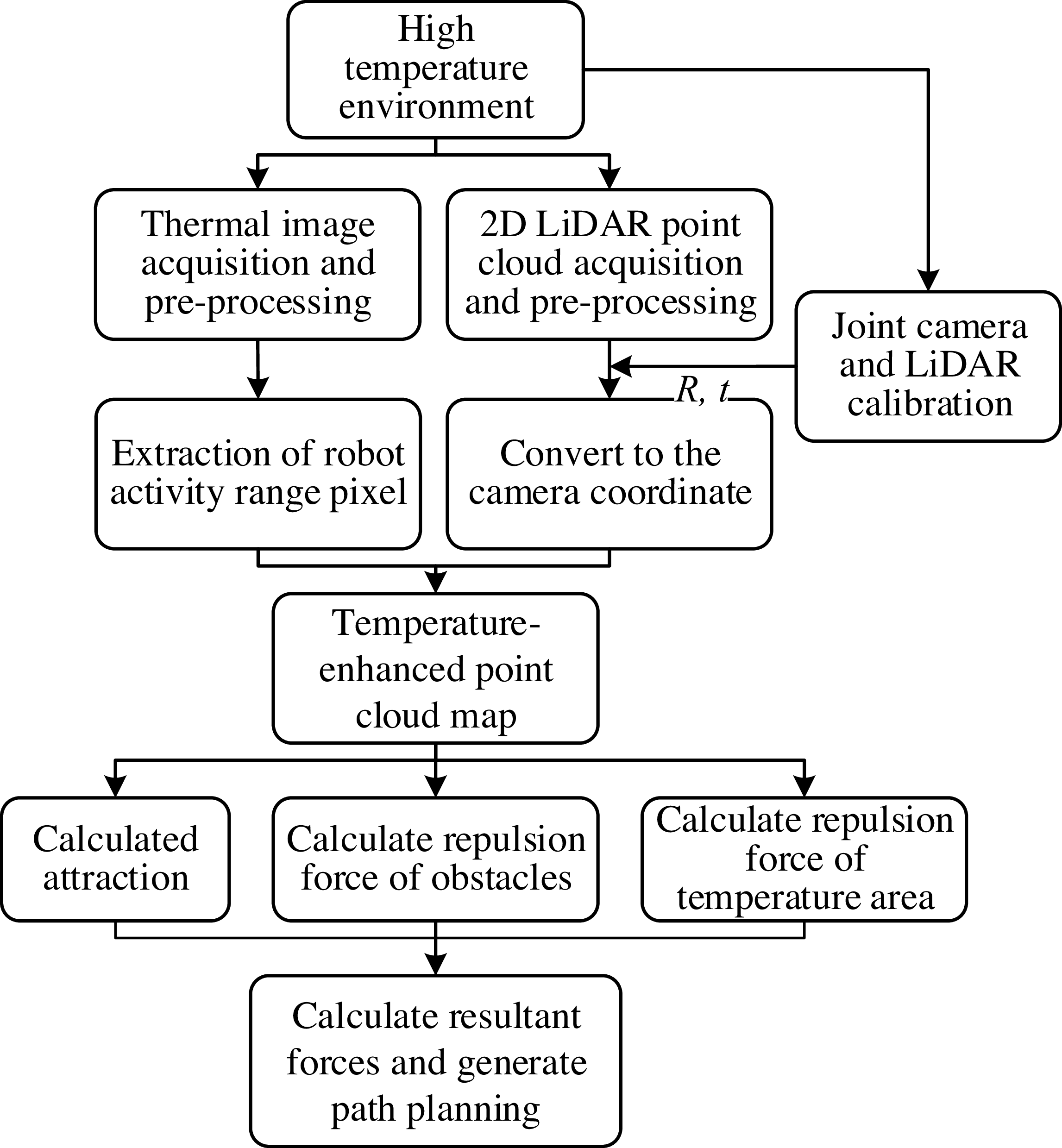
The principle of the framework is shown in Figure 1. Firstly, the internal and external parameters of the two sensors are obtained by the joint calibration method according to the obtained environmental information. The data obtained by the two sensors is then preprocessed. At the same time, the 2D LiDAR point cloud is converted to camera coordinates after pre-processing. Since the images obtained by the camera cannot be fused directly with the LiDAR, the camera point cloud is projected onto the camera’s imaging plane. Find the nearest pixel for each point cloud, add thermal information to the point cloud, and build a temperature-enhanced point cloud map. Attraction, repulsion, and temperature repulsion are calculated, respectively, to construct the overall map’s field of influence based on this point cloud map. The final path planning is realized according to the force of the force field on the robot.
Framework of the method.

Figure 1 Long description
The flowchart begins with a high-temperature environment, branching into two parallel processes: thermal image acquisition and pre-processing, and 2D LiDAR point cloud acquisition and pre-processing. These processes converge after joint camera and LiDAR calibration, leading to the extraction of robot activity range pixels and conversion to the camera coordinate. The resulting temperature-enhanced point cloud map is used to calculate attraction, repulsion force of obstacles, and repulsion force of temperature areas. These calculations feed into the final step of calculating resultant forces and generating path planning.
3.1. Thermal imager and LiDAR fusion mapping
3.1.1. Joint calibration
The data obtained by 2D LiDAR and thermal imager are based on their respective coordinate systems. In order to realize the data fusion of 2D LiDAR and thermal imager, it is necessary to unify their data into the same coordinate system, and the key is to determine the rigid coordinate transformation relationship between the two sensors.
Suppose one point P is
 $\boldsymbol{P}_{l}=(X_{l},Y_{l},Z_{l})^{T}$
in the 2D LiDAR coordinate system and is
 $\boldsymbol{P}_{t}=(X_{t},Y_{t},Z_{t})^{T}$
in the thermal imager coordinate system. The relation between
P
l
and
P
t
can be expressed as
 \begin{equation} \boldsymbol{P}_{\boldsymbol{c}}=\left(\begin{array}{l} X_{c}\\ Y_{c}\\ Z_{c} \end{array}\right)=\boldsymbol{R}\boldsymbol{P}_{\boldsymbol{l}}+\boldsymbol{t}=\boldsymbol{R}\left(\begin{array}{l} X_{l}\\ Y_{l}\\ Z_{l} \end{array}\right)+t. \end{equation}
where
R
and
t
are the rotation matrix and the offset matrix of the LiDAR coordinate system and the thermal imager coordinate system. The coordinate information of the camera space point can be represented by the pixel coordinate of the projection point
 $(u,v)$
and the depth value Z
c
of the corresponding projection point. The conversion relationship between
P
l
and camera pixel coordinates can be expressed as
 \begin{equation} \left(\begin{array}{l} u\\ v\\ 1 \end{array}\right)=\frac{1}{Z_{c}}\left(\begin{array}{l@{\quad}l@{\quad}l} f_{x} & 0 & c_{x}\\ 0 & f_{y} & c_{y}\\ 0 & 0 & 0 \end{array}\right)\left(\begin{array}{l} X_{c}\\ Y_{c}\\ Z_{c} \end{array}\right)=\frac{1}{Z_{c}}\boldsymbol{K}\left(\begin{array}{l} X_{c}\\ Y_{c}\\ Z_{c} \end{array}\right)=\frac{1}{Z_{c}}\boldsymbol{K}\left(\boldsymbol{R}\left(\begin{array}{l} X_{l}\\ Y_{l}\\ Z_{l} \end{array}\right)+\boldsymbol{t}\right). \end{equation}
where
 $f_{x}$
and
 $f_{y}$
are the focal length of the camera,
 $c_{x}$
and
 $c_{y}$
are the offset of the pixel coordinate system,
K
is the internal parameter matrix of the camera. The goal of joint calibration is to determine
K
,
R
, and
t
.
3.1.2. Coordinate transformation
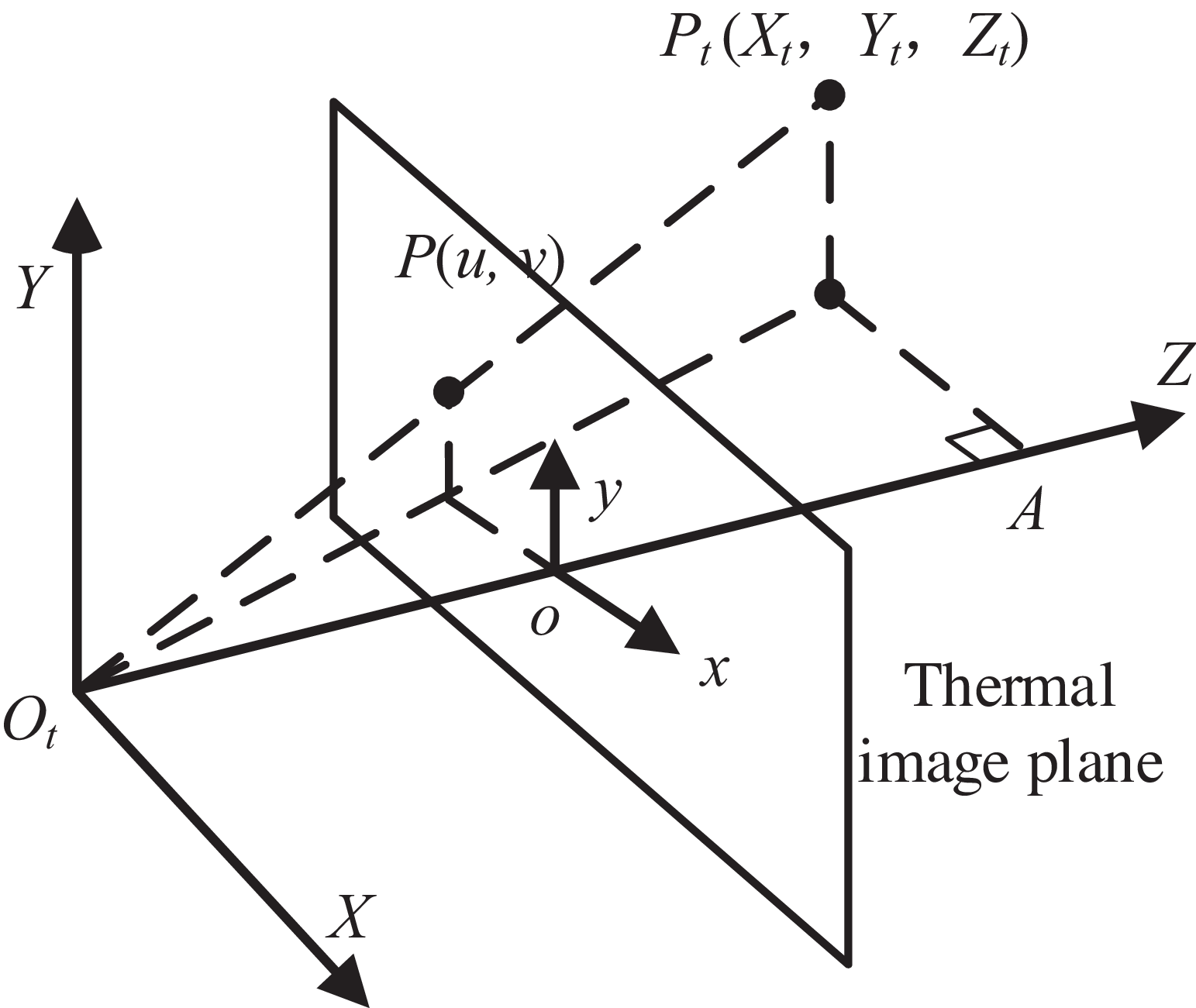
After coordinate transformation, LiDAR and thermal imager are in the same coordinate system. In order to fuse the camera point cloud and LiDAR point cloud, the radar point cloud needs to be projected onto the plane where the thermal imager map is located, as shown in Figure 2.
Camera 3D point cloud projection.

Figure 2 Long description
The diagram illustrates the projection of a 3D point cloud onto a thermal image plane. It features a coordinate system with axes labeled X, Y, and Z, and a thermal image plane intersecting these axes. Points in the 3D space, labeled as P(Xt, Yt, Zt), are projected onto the thermal image plane at positions labeled P(u, v). The diagram includes labels for the origin Ot, the thermal image plane, and the coordinates x, y, and o on the image plane. Dashed lines represent the projection of 3D points onto the 2D thermal image plane.
The coordinates of the points projected by the LiDAR point cloud onto the plane of the thermal imager map are expressed as
 \begin{equation} \left\{\begin{array}{l} u=\dfrac{f_{x}\ast X_{c}}{Z_{c}}+c_{x}\\[8pt] v=\dfrac{f_{y}\ast Y_{c}}{Z_{c}}+c_{y} \end{array}\right. .\end{equation}
The mismatch between the higher resolution of the thermal imaging image and the point cloud formed by the LiDAR is projected onto the image. This results in the LiDAR point cloud after projection being relatively sparse on the thermal imaging image. To extract temperature values from the thermal imaging image, we need to associate each LiDAR point with a pixel in the thermal imaging image. For each projection point of a single scan, the neighborhood range of the point is expanded to obtain more temperature information. After removing points that are beyond the image boundaries or have invalid depth, for each projection point of a single scan, the neighborhood range is expanded to obtain more temperature information. A circular neighborhood is extracted centered on the projection point (u, v), and the Euclidean distance of all pixels within the neighborhood to (u, v) is calculated.
 \begin{equation} d_{k}=\sqrt{\left(i_{k}-u\right)^{2}+\left(j_{k}-v\right)^{2}} .\end{equation}
The temperature value t k is extracted from the selected pixel set, and the average value t is calculated.
 \begin{equation} \left\{\begin{array}{l} t=\dfrac{\sum _{k=1}^{n}w_{k}\ast t_{k}}{\sum _{k=1}^{n}w_{k}}\\[8pt] w_{k}=exp\!\left({-}d_{k}^{2}/\sigma ^{2}\right) \end{array}\right. .\end{equation}
The temperature value t of the projection point is obtained through Gaussian weighted averaging. The weight w k is an exponential decay function of the distance from the pixel to the center point. The closer the distance, the greater the weight. The parameter σ controls the speed of the decay.
The temperature value t of these hot spots is added to the original coordinates of the point cloud projection point, denoted as
 $\boldsymbol{P}_{tl}=(X_{l},Y_{l},Z_{l},T)$
.
The result after superposition fusion is shown in Figure 3. The laser point cloud data and pixel images of the thermal imager are obtained in the same coordinate system by conversion. The data from the two sensors are superimposed and used for building temperature-enhanced point clouds.
Temperature-enhanced point cloud after sensor fusion.

Due to the different data collection frequencies of LiDAR and thermal imagers, time synchronization is required before fusion. This can be achieved through timestamp alignment. Timestamps are recorded for each LiDAR scan and thermal image frame. For each LiDAR scan frame, the thermal image frame with the closest timestamp is found.
 \begin{equation} T_{\textrm{sync}}=arg\min _{{\unicode[Arial]{x0394}} t}\parallel P_{\text{lidar}}(t)-P_{\text{thermal}}\left(t+{\unicode[Arial]{x0394}} t\right)\parallel \end{equation}
When T sync is less than the set value, data fusion is performed. If no synchronized frame is found, skip this LiDAR scan.
3.1.3. Loop closure detection in hot environments
The temperature-enhanced point cloud obtained by fusing thermal images and LiDAR sensors is used for closed-loop detection, which is applied to enhance the robustness, accuracy, and scene adaptability of the SLAM system, especially in the high-temperature environment described in this paper. During the robot’s movement, inevitable mapping accumulation errors will occur. The closed-loop detection identifies loops to provide a strong constraint for the system, pulling the current pose and historical poses together, thereby significantly correcting the global consistency of the entire trajectory and map.
In this part, we propose to use geometric-thermal joint features for the closed-loop detection part. Features of 2D LiDAR point clouds and thermal imaging data are extracted to construct geometric-thermal joint feature descriptors.
In 2D point clouds, we usually calculate geometric features using points and their neighborhoods. Here, we adopt an algorithm similar to Fast Point Feature Histogram (FPFH), but simplify it to 2D. For point p and one of its neighboring points q n , the following characteristics are calculated.
-
• The angle
 $\alpha$
between the vector
pq
n
and the tangent vector at point
p
is obtained through local linear fitting within the domain.
-
• The angle
$\beta$
between the tangent vector at point
q
n
and vector
pq
n
. -
• The angle θ between the normal vectors at point p and point q n .


Then, the angle features (
 $\alpha$
,
 $\beta$
, θ) between point
p
and each of its neighboring points are statistically analyzed to form a histogram. Each angle is divided into several intervals, and the frequency of falling into each interval is counted. Thus, each point has a geometric feature histogram. This histogram is the simplified FPFH feature of the point, which we denote as F
geom(
p
).
For each point p , not only does it have its geometric information, but thermal imaging data is fused to attach a temperature value t to each point. Therefore, the following thermal features of point p and its domain point q n are extracted.
-
– The average temperature of the neighborhood is as follows.
(7)
\begin{equation} \mu _{t}=\left(1/k\right)\ast \sum t_{i} \end{equation}
i is the index of the neighborhood points, including point p itself.
-
– The standard deviation of the neighborhood temperature is as follows.
(8)
\begin{equation} \sigma _{t}=\sqrt{\left(1/k\right)* \sum \left(t_{i}- \mu _{t}\right)^{2}} \end{equation}
-
– Divide the temperature range into several intervals, count the number of points in each temperature interval within the neighborhood, and form a neighborhood temperature distribution histogram, denoted as hist t .


These three parts combine to form a thermal feature vector F thermal( p ) = [μ t , σ t , hist t ].
The geometric feature histogram F geom( p ) and the histogram hist t in the thermal feature are also normalized. μ t and σ t are standardized using the temperature mean and standard deviation of the entire scene.
 \begin{equation} \left\{\begin{array}{l} \mu _{\text{global}}=\left(1/N\right)*\sum t_{i} \\ \sigma _{\text{global}}=\sqrt{\left(1/N\right)* \sum (t_{i}- \mu _{\text{global}})^{2}}\\ \mu '_{t}=(\mu _{t}-\mu _{\text{global}})/\sigma _{\text{global}}\\ \sigma '_{t}=\sigma _{t}/\sigma _{\text{global}} \end{array}\right. \end{equation}
μ global is the global average temperature, and σ global is the global temperature standard deviation.
The normalized geometric features and thermal features are combined into a descriptor F( p ).
 \begin{equation} F \! \left(p\right)=\left[F'_{\text{geom}}\left(p\right),F'_{\text{thermal}}\left(p\right) \right] \end{equation}
Suppose that the key frame k contains N points. The global descriptor obtained by averaging the descriptors of the N points in the key frame can be expressed as follows.
 \begin{equation} G(k)=1/N*\sum _{i=1}^{N}F(p_{i}) \end{equation}
For key frames k and c, calculate their global descriptors, respectively. Split the global descriptors into geometric and thermal parts as follows.
 \begin{equation} \left\{\begin{array}{l} G(k)=\left[G_{\text{geom}}(k),G_{\text{thermal}}(k)\right]\\[5pt] G(c)=\left[G_{\text{geom}}(c),G_{\text{thermal}}(c)\right] \end{array}\right. \end{equation}
Then, the geometric and thermal Euclidean distances are calculated separately as follows.
 \begin{equation} \left\{\begin{array}{l} d_{g}=\left\| G_{\text{geom}}(k)-G_{\text{geom}}(c)\right\| _{2}\\[6pt] d_{t}=\left\| G_{\text{thermal}}(k)-G_{\text{thermal}}(c)\right\| _{2} \end{array}\right. \end{equation}
Set the geometric distance threshold
 ${\tau}_{g}$
and the thermal distance threshold
 ${\tau}_{t}$
. When the following conditions are simultaneously satisfied
 ${{d}_{g}} \lt {\tau}_{g}$
and
 ${{d}_{t}} \lt {\tau}_{t}$
, then it is considered that the two key frames have passed the geometric-thermal consistency verification, that is, they are matched.
This method decomposes the global descriptors to independently verify the geometric and thermodynamic consistency, thereby avoiding incorrect matches in the dynamic thermal environment. Closed-loop detection of the fused thermal image and LiDAR can construct a more accurate and robust, globally consistent map.
3.2. Path planning with thermal map
3.2.1. Temperature-enhanced point cloud pretreatment
Due to the influence of hardware characteristics and detection noise, the temperature-enhanced point cloud obtained by LiDAR in thermal environment has the following problems: (1) The density of point cloud attenuates with the increase of detection distance, resulting in the overfitting of the temperature field at the near end and the loss of the features at the far end, which directly affects the accuracy of the temperature repulsion force; (2) Abnormal temperature value is introduced by sensor noise and environmental thermal disturbance, which is easy to cause path oscillation when directly used in repulsive field calculation; (3) The computational complexity of potential fields involving high-density discrete point clouds is high, which affects the computational efficiency of mobile robots. In order to alleviate the negative impact of the above problems on path generation, this paper adopts the grid method to preprocess the original point cloud.
The continuous two-dimensional space is divided into grids by fixed side lengths, each grid is identified by its index (i, j), and the central coordinate of each grid is calculated as the representative position. Each grid may contain multiple obstacle points, and the mean temperature of all points within the grid needs to be aggregated into a representative value.
 \begin{equation} T_{\text{grid}}=\frac{1}{N}\sum _{k=1}^{N}T_{ob,N} \end{equation}
If there are point clouds within the grid, each grid will be regarded as a circular obstacle. Its influence radius covers the entire grid area, ensuring that a path can be found by avoiding the grid edges.
 \begin{equation} R_{{\rm grid}}=\frac{\sqrt{\left({\unicode[Arial]{x0394}} x\right)^{2}+\left({\unicode[Arial]{x0394}} y\right)^{2}}}{2}=\frac{\sqrt{2}}{2}*L_{{\rm grid}} \end{equation}
where Δx = Δy = L grid is the side length of the grid.
Due to the closed or obstructive environment, the intensity of the heat radiated by the high-temperature grid points to the surrounding space follows the exponential attenuation model in this paper. For a single high-temperature grid heat source HS(x s , y s, T s ), the temperature value at which its thermal radiation decays to any grid (x, y) is
 \begin{equation} T\left(x,y\right)=\left\{\begin{array}{l@{\quad}l} T_{s}\cdot e^{-\lambda \cdot d\left(x,y\right)}&{\rm if}\ d\left(x,y\right)\leq r\\ 0&\text{otherwise} \end{array}\right. \end{equation}
Among them,
 $\unicode{x03BB}$
is the speed of temperature diffusion controlled by the attenuation coefficient, and
 $d(x,y)=\sqrt{(x-x_{s})^{2}+(y-y_{s})^{2}}$
is the distance from the target point to the heat source point. r is the effective radiation radius of the heat source. Beyond this range, it is considered to have no effect. If the target point is affected by multiple high-temperature grids, its temperature values are superimposed according to the radiation intensity.
This method can reduce the uncertainty of environmental modeling and provide a feasible framework for temperature sensing path planning, and its practical effect will be verified in subsequent experiments.
3.2.2. Artificial potential field
The artificial potential field method is a common method for local path planning. It is the movement of the robot in the surrounding environment, designed as an abstract artificial gravitational field movement. The target point produces “gravity” in the mobile robot, and the obstacle produces “repulsion” in the mobile robot. Finally, the motion of the mobile robot is controlled by finding the resultant force.
The artificial potential field method models the environment as a potential field. The target point is attractive to the robot, and the potential field function can be expressed as
 \begin{equation} U_{{\rm att}}(q)=\frac{1}{2}k_{att}\cdot d\left(q,q_{{\rm goal}}\right)^{2} .\end{equation}
where q is the current position of the robot, q goal is the target point, and k att is the attraction coefficient.
Obstacles generate a repulsive force on the robot, and the potential field function can be expressed as
 \begin{align} U_{{\rm rep}}(q)=\left\{\begin{array}{l@{\quad}l} \dfrac{1}{2}k_{{\rm rep}}\cdot \left(\dfrac{1}{d\left(q,q_{{\rm obs}}\right)}-\dfrac{1}{d_{0}}\right)^{2}d^{2}\left(q,q_{{\rm goal}}\right)&\text{ if }d\left(q,q_{\text{obs}}\right)\leq d_{0} \\[10pt] 0&\text{ otherwise} \end{array}\right. . \end{align}
where q obs is the position of the obstacle, d 0 is the influence range of the obstacle, and k rep is the repulsive force coefficient. The repulsive force of the obstacle does not always exist, but only occurs when the distance between the obstacle and the robot is less than the distance threshold.
3.2.3. Path planning with thermal information
By integrating the thermal information into the potential field method, the high-temperature area is regarded as an obstacle to increasing the repulsive force, and the potential field strength is dynamically adjusted according to the gradient distribution of the thermal value.
The point cloud data is converted into a raster map, and the thermal value T is assigned to each raster. The repulsive potential field in the high-temperature region can be expressed as
 \begin{equation} U_{\text{heat-rep}}(q)=\left\{\begin{array}{l@{\quad}l} \dfrac{1}{2}k_{\text{heat-rep}}\cdot \dfrac{T\left(q_{\text{heat}}\right)-T_{\text{thre}}}{\max \left(d\left(q,q_{\text{heat}}\right)^{2},d_{\text{heat-}\min }^{2}\right)}&\text{ if }T\left(q_{\text{heat}}\right)\geq T_{\text{thre}}\\ 0&\text{ otherwise} \end{array}\right. . \end{equation}
where k heat-rep is the coefficient of thermal repulsion force, T(q) is the thermal value of the high-temperature region, and T thre is the threshold of the high-temperature region. k heat-rep will adjust according to the range and importance of the thermal value and need to coordinate with the repulsive force of the obstacle to avoid conflict. The repulsive force weight is reduced at high temperatures near the target point, as follows.
 \begin{equation} k_{\text{heat-rep}}=k_{\text{heat-rep-base}}\left(1-e^{-\frac{d\left(q,q_{\text{goal}}\right)^{\beta }}{2}}\right). \end{equation}
 $\beta$
is the attenuation coefficient that controls how fast the repulsive force decays as it approaches the target. The temperature-repulsive force of the obstacle is generated only when the distance between the obstacle and the robot is less than the threshold of temperature action. Based on the empirical formula of temperature decay with distance
 \begin{equation} T_{d}=T_{0}*e^{-d/\alpha } \end{equation}
where T 0 is the temperature of the heat source and T d is the temperature at a distance d from the heat source. By substituting T thre into T d , the distance between the temperature threshold and the heat source can be expressed as
 \begin{equation} D_{\text{thre}}=\alpha *\left(\ln T_{0}-\ln T_{\text{thre}}\right) \end{equation}
The temperature-repulsive force of the obstacle only acts when the distance from the heat source is less than D thre.
After superimposing all potential fields, the total potential field function can be expressed as
 \begin{equation} U_{\text{total}}(q)=U_{\text{att}}(q)+U_{\text{rep}}(q)+U_{\text{heat-rep}}(q) \end{equation}
Gradient descent is used to find a path from the starting point to the target point in the total potential field.
 \begin{equation} q_{\text{next}}=q_{\text{current}}-\nabla \ast U_{\text{total}} (q_{\text{current}}) \end{equation}
The potential field coefficients k rep and k heat-rep are adjusted to achieve a balance between obstacle avoidance and thermal constraints. Through the above method, the point cloud map based on thermal information and the artificial potential field method can be realized.
In the process of path generation based on the potential field method, although the introduction of the discretization step guarantees the convergence of the algorithm, it inevitably leads to the non-smooth oscillation of the path. This paper uses the Savitzky–Golay filter for path smoothing, which is a smoothing algorithm based on local polynomial fitting. The core idea is to preserve the characteristics of the signal by polynomial fitting in the sliding window while suppressing noise-induced fluctuations. The SG filter maintains the geometry of the signal while smoothing.
For the path sequence Q = {q 1, q 2, …, q n }, the polynomial is fitted in the sliding window, and the formula is as follows.
 \begin{equation} \begin{cases} x(t)=a_{0}+a_{1}t+a_{2}t^{2}+\cdots +a_{k}\hspace{0pt}t^{k}\\ y(t)=b_{0}+b_{1}t+b_{2}t^{2}+\cdots +b_{k}\hspace{0pt}t^{k} \end{cases} \end{equation}
where t is the local time coordinate in the window and k is the polynomial order. The coefficients {a k }, {b k } are solved by the least square method, and the value of the fitting polynomial at the center point of the window is used as the smoothed output. The filtered coordinates can be expressed as
 \begin{equation} Q_{\text{smooth}}=SG\_ \text{Filter} (Q,k,w) \end{equation}
where k is the polynomial order, representing the highest degree of fitting the polynomial and w is the window size representing the sum of the current points used in each fit and the number of points before and after them. The smoothed path after fitting is shown in Figure 4.
The original path and smooth path are represented by the red dotted line and the blue solid line, respectively.

Figure 4 Long description
A scatter plot displays a collection of data points with a red dotted line and a blue solid line representing different paths. The red dotted line indicates the original path, while the blue solid line represents the smooth path. The plot includes a legend in the top right corner, identifying the start and end points with blue and green dots, respectively. The x-axis and y-axis represent numerical values, with the data points scattered across the plot. The plot shows clusters of points and distinct paths, illustrating the comparison between the original and smooth paths. All values are approximated.
The pseudocode of the path-planning algorithm with thermal map is shown below.
Temperature-enhanced Artificial Potential Field Path Planning.

Algorithm 1 Long description
The pseudocode outlines a path-planning algorithm that incorporates thermal maps. It starts with initializing the path and current position. The algorithm iterates to update the path by calculating attractive and repulsive forces from obstacles and thermal influences. It checks for convergence and updates the current position accordingly. The process repeats until the maximum number of iterations is reached or the goal is achieved.
4. Case study
In this paper, the mobile robot platform based on the Ubuntu system is adopted. The platform is equipped with RPLIDAR-A2 LiDAR and Hikmicro thermal imager, which are shown in Figure 5.
The mobile robot platform.

Figure 5 Long description
The image shows a mobile robot platform with several labeled components. The 2D LiDAR is positioned at the front center of the platform. To the right, there is a thermal imager mounted on a raised structure. On the left side, a mobile control module is visible, and at the back, an industrial personal computer is placed. The robot is equipped with four wheels, each featuring a unique tread pattern designed for mobility. The platform appears to be on a carpeted surface, and various cables and connectors are visible, indicating the integration of different electronic components.
4.1. Temperature-enhanced point cloud map
The thermal image obtained by the thermal imager and the point cloud data obtained by 2D LiDAR are, respectively, in their coordinate systems. The thermal image and 2D point cloud are shown in Figure 5 above.
The infrared thermal image with a resolution of 512 × 384 output by the thermal imager is shown in Figure 6(a). Each pixel contains radiation intensity information, which is converted into a temperature value according to parameters. The horizontal field of view Angle of the single-line LiDAR is 270°, and the angular resolution is 0.25°, as shown in Figure 6(b). The generated two-dimensional polar coordinate point cloud is expressed as {(r i , θ i )(x i , y i )} after Cartesian coordinate conversion.
Thermal images (a), 2D point clouds (b), and physical photo (c).

Figure 6 Long description
The image consists of three distinct elements: thermal images, 2D point clouds, and a physical photo. The thermal images (a) display heat distribution in a room, with color gradients indicating temperature variations. The 2D point clouds (b) show the spatial mapping of the environment, with red lines representing the planned paths. The physical photo (c) depicts a room with a robot and a heater, providing a real-world context for the path planning scenario. These elements are combined to highlight the integration of thermal and geometric data for effective path planning in high-temperature environments, addressing the challenges faced by traditional methods that rely solely on geometric obstacle information.
After the joint calibration, the data of the two sensors are unified in a spatial coordinate system. The pixel information of the thermal image is converted into temperature information, and the temperature information of the thermal imager is embedded in the LiDAR point cloud to generate a two-dimensional temperature-enhanced point cloud map. After fusion, the point cloud format is (x, y, T). The two-dimensional temperature point cloud image after fusion is shown in Figure 7.
Temperature-enhanced point cloud map. Point color depth corresponds to temperature value (dark red → high temperature, dark blue → low temperature).

Figure 7 Long description
A heat map displays temperature variations in a point cloud map. The color depth of the points corresponds to temperature values, with dark red indicating high temperatures and dark blue indicating low temperatures. The map features a grid layout with varying temperature intensities across different regions. The temperature scale ranges from 15.2 to 100.9 degrees. Notable regions include areas with higher temperature values marked in red and lower temperature values marked in blue. The overall structure shows a distribution of temperature points with distinct clusters and gradients.
4.2. Improved artificial potential field method
To verify the robustness of the improved artificial potential field method based on temperature-enhanced point cloud maps in thermal environments, experiments were conducted in three typical scenarios:
-
1. Family-living environment: there are both localized high-temperature zones generated by heating appliances and thermal regions to mimic electrical overload scenarios. There are several fixed high-temperature points distributed in the environment (T ≈ 90 °C).
-
2. Continuous casting workshop: there are several steelmaking furnaces with different high temperatures (T > 100°C).
-
3. Steelmaking scrap area: there are unstructured barriers to stacking metal waste (T ∈ [50, 300]°C).
The actual environment of these three scenarios is shown in Figure 8.
Three scenarios: (1) family-living environment; (2) continuous casting workshop; (3) steelmaking scrap area.

Figure 8 Long description
The image contains three separate photos. The first photo shows a family-living environment with a heater on the floor. The second photo depicts a continuous casting workshop with large industrial equipment and machinery. The third photo illustrates a steelmaking scrap area with piles of scrap metal and industrial structures. These scenarios demonstrate different environments where advanced robotic perception capabilities, such as LiDAR and thermal imagers, can be applied to sense environmental information and adapt to various mission requirements.
In scenario 1, the point cloud with temperature information is collected by the mobile robot, as shown in Figure 9 above. The heat source here is mainly electric heating, air heaters, and simulated overload electrical appliances.
Temperature-enhanced point cloud map in the family-living environment.

Figure 9 Long description
The image displays a temperature-enhanced point cloud map of a family-living environment. The map uses different colors to represent varying temperatures, with blue indicating cooler areas and yellow to red indicating warmer areas. The layout of the environment includes walls, doorways, and furniture, with temperature variations highlighted across different sections.
Now the space is divided into grids, the temperature within each grid is averaged, and the repulsive force is calculated based on the grid. The goal is to reduce the amount of computation while reducing the impact of density. The attraction coefficient and repulsion coefficient are adjusted to adapt to the current environment.
Due to the hardware temperature requirements of each component of the robot, the threshold temperature T
thre is set at 40 °C. k
att represents the gravitational gain, which controls the magnitude of the attraction force exerted by the target point on the robot. The larger the value, the stronger the gravitational force, and the more ``urgently’’ the robot will head towards the target. k
rep is the basic repulsive force gain, which controls the magnitude of the repulsive force generated by ordinary obstacles (regardless of temperature). The larger the value, the more ``repelled’’ it is by the obstacle, and the path will be further away from the obstacle. Due to the introduction of the temperature repulsion force, k
rep should be smaller than the traditional APF. k
heat-rep is the base value gain of the temperature-repulsive force. It controls the absolute intensity of the temperature-repulsive force. The larger the value, the stronger the additional repulsive force generated by the high-temperature obstacle.
 $\beta$
is the temperature-repulsive force attenuation coefficient, which controls the rate at which the temperature-repulsive force decays with distance. The larger
 $\beta$
is, the faster the attenuation is, and the more concentrated the influence range of the high-temperature-repulsive force is.
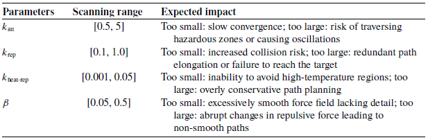
The single-parameter scanning analysis method is adopted. The traditional APF parameters are referenced, and one parameter is changed within a reasonable range. After fixing three parameters, multiple simulations are conducted to observe their impact on performance indicators, as shown in Table I.
The influence of parameters on performance indicators.

Table I Long description
The table presents the influence of parameters on performance indicators, focusing on four key parameters: k att, k rep, k heat-rep, and beta. Each parameter has a specified scanning range and expected impact on performance. The table has four rows and three columns. The first column lists the parameters: k att, k rep, k heat-rep, and beta. The second column details the scanning ranges: k att ranges from 0.5 to 5, k rep ranges from 0.1 to 1.0, k heat-rep ranges from 0.001 to 0.05, and beta ranges from 0.05 to 0.5. The third column describes the expected impacts: k att being too small causes slow convergence and too large risks traversing hazardous zones or causing oscillations; k rep being too small increases collision risk and too large results in redundant path elongation or failure to reach the target; k heat-rep being too small leads to inability to avoid high-temperature regions and too large results in overly conservative path planning; beta being too small causes excessively smooth force field lacking detail and too large results in abrupt changes in repulsive force leading to non-smooth paths.
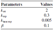
Finally, the detailed parameter settings under scenario 1 are shown in Table II. The selected parameter values have been proven to achieve the best balance between path safety (minimizing high-temperature exposure) and path efficiency (shortest feasible length).
Final parameters.

Table II Long description
A table with two columns labeled Parameters and Values. The Parameters column lists four items: kain, krep, knei-rep, and beta. The Values column shows the corresponding values: 2, 0.3, 0.005, and 0.1 respectively. The table presents numerical data in a structured format.
Based on the grid map, an improved artificial potential field method is used for path planning. As shown in Figure 10, under the combined action of attractive and repulsive forces, the planned path can successfully avoid the high-temperature heat source. The final generated path uses the Savitzky–Golay filter to smooth the planned path, as shown in Figure 11. The variation curves of attraction, repulsion, and resultant force with the increase of iterations are shown in Figure 12. Temperature repulsion plays an important role in planning.
Gridded temperature potential field path planning. The blue dot is the starting point, and the green dot is the end point. The green, red, and blue arrows represent attraction, repulsion, and resultant force, respectively.

Figure 10 Long description
Two graphs illustrate temperature potential field path planning. Each graph features a blue dot as the starting point and a green dot as the endpoint. Green arrows indicate attraction, red arrows indicate repulsion, and blue arrows represent the resultant force. The temperature scale ranges from 20 to 100 degrees Celsius, with colors transitioning from blue to red. The path planning involves navigating through varying temperature fields, with the resultant force guiding the path from start to end. All values are approximated.
Final path planning result and force variation with thermal repulsion.

Figure 11 Long description
The image contains two graphs. The first graph on the left shows the final path planning result with a start point, an end point, and a smooth path. The temperature is represented by a color gradient ranging from blue to red, indicating temperatures from 20 to 100 degrees Celsius. The second graph on the right illustrates the force variation with thermal repulsion over iteration steps. It includes four lines representing attraction, total repulsion, thermal repulsion, and the resultant force. The force magnitude is plotted on the y-axis, and the iteration steps are on the x-axis. The attraction force is shown in green, total repulsion in red, thermal repulsion in orange, and the resultant force in blue. The graphs together demonstrate how thermal repulsion affects the path planning process.
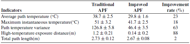
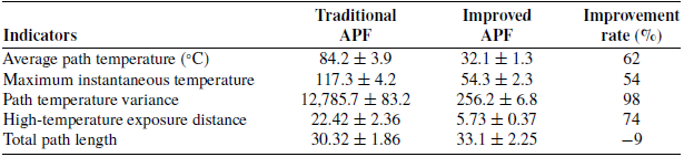
To verify the performance of the algorithm in the scenario, 15 independent experiments were conducted to ensure the reliability of the results. The underlying geometric parameters (such as step length and obstacle influence distance) of the traditional APF and this improved method were kept consistent to fairly compare the performance gain after the introduction of the temperature field. The statistical results of multiple experiments and related performance indicators are recorded, and a comparison is made with the traditional APF, as shown in the table below (Table III).
Compared with the traditional APF, the improved method successfully reduced the working path temperature by 20% and significantly reduced the risk of high-temperature exposure, while the actual path length increased only slightly.
Change different starting and ending points for path planning. The resulting path and force diagram are shown in Figure 12.
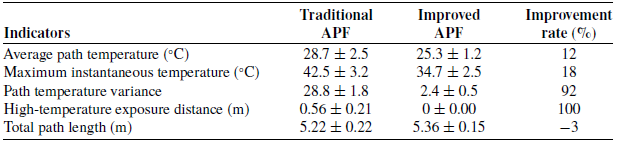
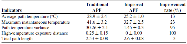
Then, 15 independent experiments are conducted in the home environment. The statistical results of multiple experiments and related performance indicators are recorded, and a comparison is made with the traditional APF, as shown in Tables IV and V below.
The improved method successfully planned paths that completely avoided the core area of high temperature in all 15 trials, achieving almost 100% elimination of high-temperature exposure.
In scenario 2, the mobile robot collects the enhanced point cloud, as shown in Figure 13. The heat source here is mainly the converter steelmaking furnace with residual temperature.
Comparison of performance indicators for path planning in the family-living environment.

Table III Long description
The table presents a comparison of performance indicators for traditional and improved Artificial Potential Field (APF) methods in path planning within a family-living environment. It includes five key indicators: average path temperature, maximum instantaneous temperature, path temperature variance, high-temperature exposure distance, and total path length. The table has five rows for indicators and three columns for Traditional APF, Improved APF, and Improvement rate. Traditional APF shows higher values in average path temperature, maximum instantaneous temperature, path temperature variance, and high-temperature exposure distance compared to Improved APF. The improvement rate column highlights significant reductions in these values with the improved method, with the highest improvement rate of 88 percentage in high-temperature exposure distance. The total path length shows a minor improvement of 2 percentage.
Comparison of performance indicators for path planning in the family-living environment.

Table IV Long description
The table compares performance indicators for path planning in a family-living environment between traditional APF and improved APF methods. It consists of five rows and four columns. The columns are labeled Indicators, Traditional APF, Improved APF, and Improvement rate percentage. The rows detail the following indicators: Average path temperature in degrees Celsius, Maximum instantaneous temperature in degrees Celsius, Path temperature variance, High-temperature exposure distance in meters, and Total path length in meters. Notable trends include a 12 percentage improvement in average path temperature, an 18 percentage improvement in maximum instantaneous temperature, a 92 percentage improvement in path temperature variance, a 100 percentage improvement in high-temperature exposure distance, and a 3 percentage decrease in total path length.
Final path planning result and force variation of two different starting and ending points.

Figure 12 Long description
The image contains two sets of graphs. The left side of each set displays a path planning result with a temperature map, showing a start point, an end point, and a smooth path. The right side of each set shows a line graph depicting force variation with thermal repulsion over iteration steps. The first set of graphs has a temperature range from 20 to 100 degrees Celsius and force magnitudes up to 6 Newtons. The second set has a temperature range from 20 to 100 degrees Celsius and force magnitudes up to 2.5 Newtons. Each force variation graph includes lines for attraction, total repulsion, thermal repulsion, and resultant forces.
Comparison of performance indicators for path planning in the family-living environment.

Table V Long description
The table compares performance indicators for path planning in a family-living environment between traditional APF and improved APF methods. It consists of five rows and four columns. The columns are labeled Indicators, Traditional APF, Improved APF, and Improvement rate percentage. The rows detail the following indicators: Average path temperature in degrees Celsius, Maximum instantaneous temperature in degrees Celsius, Path temperature variance, High-temperature exposure distance, and Total path length. Notable trends include a 13 percentage improvement in average path temperature, a 23 percentage improvement in maximum instantaneous temperature, a 95 percentage improvement in path temperature variance, a 100 percentage improvement in high-temperature exposure distance, and a 3 percentage decrease in total path length. The data highlights significant improvements in temperature-related indicators and exposure distance with the improved APF method.
Based on the grid map, an improved artificial potential field method is used for path planning. Under the combined action of attractive and repulsive forces, the planned path can successfully avoid the high-temperature heat source. The final generated path is shown in Figure 14. The variation curves of attraction, repulsion, and resultant force with the increase of iterations are shown in Figure 14. Considering the high temperature in the environment, the repulsive force in path planning is almost the only repulsive force of temperature.
Then, 15 independent experiments are conducted in the continuous casting workshop. The statistical results of multiple experiments and related performance indicators are recorded, and a comparison is made with the traditional APF, as shown in Tables VI and VII below.
Temperature-enhanced point cloud map in the continuous casting workshop.

Figure 13 Long description
The image displays a temperature-enhanced point cloud map of a continuous casting workshop. Various structures and equipment within the workshop are represented as scattered points, with different colors indicating temperature variations. The map highlights the spatial arrangement and thermal characteristics of the workshop environment, providing a detailed visualization for analysis and monitoring purposes.
Compared to the traditional APF, the improved method successfully reduces the temperature of the working path in the factory environment by 50%-60% and greatly reduces the risk of high-temperature exposure, with a small and negligible increase in the actual path length.
In scenario 3, the mobile robot collects the enhanced point cloud, as shown in Figure 15. The heat source here is mainly waste from the steelmaking process.
Based on the grid map, an improved artificial potential field method is used for path planning. Under the combined action of attractive and repulsive forces, the planned path can successfully avoid the high-temperature heat source. The final generated path is shown in Figure 16. The variation curves of attraction, repulsion, and resultant force with the increase of iterations are shown in Figure 16. Considering the high-temperature waste in the environment, the repulsive force in path planning is almost the only repulsive force of temperature.
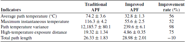
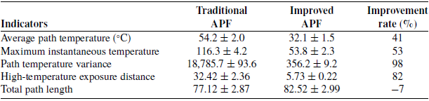
Fifteen independent experiments are conducted in the steelmaking scrap area. The statistical results of multiple experiments and related performance indicators are recorded, and a comparison is made with the traditional APF, as shown in Table VIII below.
Comparison of performance indicators for path planning in the continuous casting workshop.

Table VI Long description
The table compares performance indicators for path planning in the continuous casting workshop using traditional and improved APF methods. It consists of five rows and four columns. The columns are labeled Indicators, Traditional APF, Improved APF, and Improvement rate percentage. The rows detail various metrics: Average path temperature in degrees Celsius, Maximum instantaneous temperature in degrees Celsius, Path temperature variance, High-temperature exposure distance, and Total path length. Notable trends include significant improvements in average path temperature, maximum instantaneous temperature, path temperature variance, and high-temperature exposure distance with the improved APF method, while the total path length shows a decrease in performance.
Comparison of performance indicators for path planning in the continuous casting workshop.

Table VII Long description
The table compares performance indicators for traditional and improved APF methods in a continuous casting workshop. It has five rows and four columns, including indicators such as average path temperature, maximum instantaneous temperature, path temperature variance, high-temperature exposure distance, and total path length. The columns are labeled Traditional APF, Improved APF, and Improvement rate percentage. Notable trends include significant improvements in average path temperature, maximum instantaneous temperature, path temperature variance, and high-temperature exposure distance with the improved APF method, while the total path length shows a slight decrease.
Final path planning result and force variation of two different starting and ending points.

Figure 14 Long description
The image contains two sets of graphs. Each set includes a path planning diagram and a force variation graph. The path planning diagrams show a start point marked in blue, an end point marked in green, and a smooth path in blue. The background of the path planning diagrams is a temperature map ranging from blue (50 degrees Celsius) to red (200 degrees Celsius). The force variation graphs display the changes in force magnitude over iteration steps, with different lines representing attraction in green, total repulsion in red, thermal repulsion in orange, and resultant forces in blue. The force variation graphs show how these forces interact and change over the iteration steps, providing insights into the dynamics of the system. All values are approximated.
Comparison of performance indicators for path planning in the steelmaking scrap area.

Table VIII Long description
The table presents a comparison of performance indicators for path planning in the steelmaking scrap area, focusing on traditional and improved Artificial Potential Field (APF) methods. It includes five key indicators: average path temperature, maximum instantaneous temperature, path temperature variance, high-temperature exposure distance, and total path length. The table has five rows for these indicators and three columns for traditional APF, improved APF, and improvement rate. Notable trends include significant improvements in average path temperature, maximum instantaneous temperature, and high-temperature exposure distance with the improved APF method, showing reductions of 41 percentage, 53 percentage, and 82 percentage respectively. The path temperature variance also shows a substantial improvement of 98 percentage. However, the total path length slightly increases by 7 percentage with the improved method.
Temperature-enhanced point cloud map in the steelmaking scrap area.

Figure 15 Long description
A temperature-enhanced point cloud map in the steelmaking scrap area. The map displays a scatter plot of data points representing various locations within the steelmaking scrap area. The x-axis and y-axis represent spatial coordinates, with values estimated based on LiDAR data. The data points are color-coded to indicate temperature variations, with a gradient ranging from blue to red. The map shows clusters of points forming the outline of structures and equipment within the area. A central line, highlighted in different colors, likely represents a path or a significant feature within the scrap area. The overall pattern suggests a detailed and accurate mapping of the environment, useful for navigation and localization purposes.
Final path planning result and force variation with thermal repulsion.

Figure 16 Long description
The image contains two separate graphs. The first graph on the left is a path planning result, showing a start point, an end point, and a smooth path in blue. The x-axis represents temperature in degrees Celsius, ranging from negative one hundred to zero, while the y-axis represents an unspecified metric ranging from negative two hundred and forty to negative one hundred and eighty. The second graph on the right illustrates force variation with thermal repulsion, displaying four lines: attraction in green, total repulsion in red, thermal repulsion in orange, and resultant in blue. The x-axis represents iteration steps from zero to two thousand, and the y-axis represents force magnitude in Newtons, ranging from negative ten to fifty. The graphs are not overlaid but are presented side by side to compare different aspects of the data.
In a larger environment, the modified method successfully reduced the operating path temperature by 40% and substantially reduced the risk of high-temperature exposure, with a modest increase in the actual path length.
The effectiveness and robustness of the improved artificial potential field method based on temperature-enhanced point cloud map in thermal environment path planning are proved through the experimental verification of three typical scenarios: home life, continuous casting workshop, and steelmaking waste area. Experiments show that the algorithm can effectively avoid local high-temperature sources and generate safe and smooth paths in both structured and unstructured environments. In high-temperature industrial scenarios, the temperature repulsion contribution accounts for the main proportion and becomes the main driving force for obstacle avoidance. Compared with the traditional APF method, the improved method successfully reduces the operating path temperature by 20–60%, and greatly reduces the risk of high-temperature exposure, which verifies the necessity of the thermal environment potential field model.
4.3. Discussion
There still exist many works worthy of further investigation. Only the feasibility of avoiding high temperatures is considered, and how to determine the repulsive force for different heat sources needs further study. This planning method does not analyze the avoidance of dynamic heat sources and the transient change of the temperature field.
Based on these problems, the following research can be conducted from the following aspects. Parameters based on deep reinforcement learning are considered to be adaptive to different environments. Then, the existing model is improved to enhance the real-time performance of the algorithm.
5. Conclusion
This paper presents an improved potential field method for the path planning of mobile robots in thermal environments based on temperature-enhanced point cloud maps. This paper presents an improved potential field method for the path planning of mobile robots in thermal environments based on temperature-enhanced point cloud maps. The temperature-enhanced point cloud map is generated by combining LiDAR and thermal imaging, and the repulsive potential field function of heat radiation is introduced to realize robot path planning based on the traditional artificial potential field method. The reliability of the proposed method is verified by collecting environmental data and conducting experiments. This study provides a new idea for robot autonomous navigation under high-temperature and high-risk environments.
In the future, the direction of our next work will adopt 3D LiDAR instead of 2D LiDAR and inherit the fusion framework of this paper. It will be investigated how thermal textures can be effectively mapped onto 3D point clouds to construct a fully 3D fusion map and enable path planning. The grid map framework for probabilistic heat occupancy is adopted to consider further, and a novel method of adding heat data to update rules will be developed to improve the current method. Dynamic temperature field prediction and multi-sensor information will be further integrated to cope with more complex time-varying thermal environment challenges.
Data availability statement
The data that support the findings of this study are available from the corresponding author upon reasonable request.
Authors contribution
Yunzhi Li: Conceptualization, Methodology, Writing – original draft, Writing – review and editing; Libin Tan: Conceptualization, Writing – review and editing; Xiangrong Xu: Writing – review and editing; Zequn Zhang: Funding acquisition. All authors had approved the final version.
Financial support
This work was supported by the National Natural Science Foundation of China (52305539), the Natural Science Foundation of Jiangsu Province (BK20230880), and the China Postdoctoral Science Foundation (2023M731661).
Competing interests
The authors declare that they have no known competing financial interests or personal relationships that could have appeared to influence the work reported in this paper.
Ethical and informed consent for data used
This paper was done by the authors, and no human participants other than the authors were involved in it, and informed consent was obtained from all authors.